Foundations of a Universal Theory of Relativity

Abstract

Earlier, we had presented heuristic heuristic arguments to show that a natural unification of the ideas of the quantum theory and those underlying the general principle of relativity is achievable by way of the measure theory and the theory of dynamical systems. Here, in Part I, we provide the complete physical foundations for this, to be called, the Universal Theory of Relativity. Newton’s theory and the special theory of relativity arise, situationally, in this Universal Relativity. Explanations of quantum indeterminacy are also shown to arise in it. Part II provides its mathematical foundations. One experimental test is also discussed before concluding remarks.

To be submitted to:

The organization of this paper is such that physical foundations of the proposed Universal Theory of Relativity are to be found in §  I, its mathematical foundations in §  II, one experimental test in § III and concluding remarks in § IV.

In §  I.1, we discuss the general background for the present considerations. It should help distinguish the proposed Universal Theory of Relativity from various other theories, including, Quantum Geometry ashtekar1 and String Theory strings .

In §  I.2, we discuss the physical basis of some of the newtonian concepts, in particular, inertia and force. In this discussion, we mainly stress that the Galilean concept of the inertia of a material body is, undoubtedly, more fundamental, more general, than the newtonian concept of force. Therefore, we may expect the concept of inertia to necessarily find a place in any future physical theory, but not the concept of force.

Newton’s theory does not explain the origin of either the inertia or the electric charge of material bodies. For any theory that attempts to explain the origin of inertia and the electric charge, it then becomes necessary to replace the newtonian concept of force with some suitable other. The concept of the material body as a source of force is, consequently, to be completely abandoned in any such theoretical framework. Decisively, this must, simultaneously, hold for all the forces that need to be postulated to describe the motions of material bodies in Newton’s and other theories.

In other words, it is decisive to recognize that the mathematical framework of any theory which “explains” origins of newtonian source properties of the physical matter must, necessarily, be also applicable, simultaneously, to all the “fundamental” forces that are needed in Newton’s and other theories to describe the motions of material bodies. This is heuristic the key to the “new” theory.

Clearly, a formulation that replaces the concept of only a single source property of material bodies cannot then be physically satisfactory as well as conceptually consistent.

In this section, we then stress the importance of the physical construction of the reference frames or the coordinate systems. We also stress that the motions of material bodies must, in general, affect the constructions of coordinate frames.

In §  I.3, we then discuss the status of the general principle of relativity. This important principle states that the laws of physics must be applicable to all the frames of reference. Consequently, the universal theory of relativity, a theory consistent with the general principle of relativity, will necessarily have to incorporate the physical construction of the coordinate systems.

In the context of this above discussion, we also consider Einstein’s equivalence principle and stress that the equivalence principle essentially establishes only the consistency of the phenomenon of gravitation with the general principle of relativity. It then needs to be emphasized here that the equivalence principle is not logically equivalent to the general principle of relativity.

In section §  I.4, we discuss various general expectations from a theory consistent with the general principle of relativity. This section essentially sets the conceptual background for the sections to follow. But, a reader is requested to go through even the earlier sections.

Then, in §  I.5, we consider quantum aspects heisenberg vis-$\acute{a}$-vis the general principle of relativity and the requirements of the mathematical formalism implied by such considerations.

In §  II, we provide the mathematical foundations for the proposed unified theory. Specifically, methods of measure theory and dynamical systems are reviewed in this section.

Then, in § III, we analyze a torsion balance experiment. Any theory using the concept of force always predicts a non-null effect for this experiment. However, a “null effect” is also obtainable in the Universal Theory of Relativity apart from possible non-null effects (of the theories using the concept of force). We therefore suggest that the existence of such anomalous null-results be searched for in torsion balance experiments, preferably involving dynamic measurements.

[Such anomalous null results will be some of the main features of the proposed Universal Theory of Relativity. This is because a transformation of the underlying space providing null result for any given experimental situation is, thinkably, permissible. But, physical space of Universal Relativity changes with changes in matter. Care is therefore needed in establishing null-results.]

Finally, §  IV, contains some concluding remarks about the proposed theory.

I PHYSICAL FOUNDATIONS

I.1 General Background

For the sake of completeness, we recall here the discussion from heuristic . Its purpose here is to contrast the present approach with some other approaches ashtekar1 ; strings to the unification of the ideas of the quantum theory and Einstein’s general relativity.

In an essence, Newton’s deliberations define cartan specific mathematical structures or fields (scalar, vector, tensor functions) over the metrically flat 3-continuum and consider the laws of their transformations. The 3-continuum admits the same Euclidean metric structure before and after the coordinate transformations. The ever-flat 3-continuum is, in this sense, an absolute space and, in Newton’s theory, accelerations of material bodies can refer only to this absolute space.

Furthermore, in Newton’s theory, physical laws for these quantities are the mathematical statements form-invariant under the galilean coordinate transformations which are basic to the newtonian formulation of mechanics.

Mathematical methods class-mech for these newtonian fields are, evidently, required to be consistent with the underlying flat 3-continuum admitting the same metric structure before and after the transformations of these fields. This is, truly, the sense of any theory being newtonian.

Then, the galilean transformations under which the newtonian laws are form-invariant are, as opposed to general, specific transformations of the coordinates of the continuum $\mathbb{R}^{3}$.

Newton’s theory also attaches physical meaning to the space coordinates and to the time coordinate. In this theory, the space coordinate describes the “physical distance” separating physical bodies and the time coordinate describes the reading of a “physical” clock. Euclidean space is then also the physical space of Newton’s theory.

In addition, the (newtonian) temporal coordinate has universally the same value for all the spatial locations, ie, all synchronized clocks at different spatial locations show and maintain the same time. In other words, the newtonian time coordinate is the absolute physical time.

Basically, Newton’s theory imagines a material body as a point-mass endowed with the inertia of that material body. It is a primary physical conception of this theory. Necessarily, a point-mass moves along a one-dimensional curve of the unchanging Euclidean 3-continuum.

In physical associations of Newton’s theory, it is then tacitly assumed that the interaction of a measuring instrument (observer) and the object (a particle whose physical parameters are being measured) is negligibly small or that the effects of this interaction can be eliminated from the results of observations to obtain, as accurately as desired, the values of these parameters bohr1 .

An issue closely related to the above one is that of the causality. Given initial data, Newton’s theory predicts the values of its variables of the point-mass exactly and, hence, assumes strictly causal development of its physical world.

Conceptually, in Newton’s theory, force is the cause behind motions of material bodies. Next to inertia, force is the second most important of the conceptions of Newton’s theory.

Furthermore, as Lorentz had first realized very clearly, the sources of the newtonian forces are the singularities of the corresponding fields defined on the flat 3-continuum. Although unsatisfactory, this nature of the newtonian framework causes no problems of mathematical nature since this distinction is maintainable within the formalism, ie, well-defined mathematical procedures for handling this distinction are possible.

Here, one could imagine bodies of vanishing inertia moving with the same speed relative to all the inertial observers. But, acceleration (relative to absolute space) in Newton’s second law of motion has no meaning for vanishing inertia. This inability is a certain indication of the limitations of Newton’s theoretical framework.

Then, if a zero rest-mass object were to exist in reality, and nothing in Newton’s theory prevents this, it is clear that we need to “extend” various newtonian conceptions. Only experiments can tell us about the existence of such bodies.

Now, light displays phenomena such as diffraction, interference, polarization etc. But, as is well known, Newton’s corpuscular theory needs unnatural, non-universal, inter-particle forces to explain these phenomena. That light displays phenomena needing unnatural explanations in Newton’s theory could, with hindsight, then be interpreted 100-yrs to mean that light needs to be treated as a zero rest-mass particle. Then, the speed of Light is the same for all the inertial observers.

Revisions of newtonian concepts were necessary by the beginning of the 20th century. Firstly, efforts to reconcile some experimental results with newtonian concepts failed and associated as well as independent conceptions led Einstein to Special Theory of Relativity ein-pop . Secondly, other experiments related to the wave-particle duality, of radiation and matter, both, ultimately led to non-relativistic quantum theory heisenberg .

The methods of Non-Relativistic Quantum Field Theory qt are also similar of nature to the above newtonian methods in that these consider quantum fields definable on the metrically flat 3-continuum. For these fields of quantum character, we are of course required to modify the newtonian mathematical methods. The Schrödinger-Heisenberg formalism achieves precisely this.

Quantum considerations only change the nature of the mathematical (field) structure definable on the underlying metrically flat 3-continuum. That is, differences in the newtonian and the quantum fields are mathematically entirely describable as such. But, the metrically flat 3-continuum is also, in the above sense, an absolute space in these non-relativistic quantum considerations.

Now, importantly, the “newtonian source properties” of physical matter are differently treated in the non-relativistic quantum field theory than in Newton’s theory. The mass and the electric charge of a physical body appear as pure numbers, to be prescribed by hand for a point of the metrically flat 3-continuum, in Schrödinger’s equation or, equivalently, in Heisenberg’s operators.

Quantum theory then provides the probability of the location of the mass and the charge values in certain specific region of the underlying metrically flat 3-continuum. The mathematical formalism of the quantum theory provides only probability and it is basically a set of mathematical rules to calculate the probability of a physical event.

However, certain physical variables of the newtonian mass-point acquire discrete values in the mathematical formalism of the quantum theory. This discreteness of certain variables is the genuine characteristic of the quantum theory and is a significant departure from their continuous values in Newton’s theory.

This quantum theory is fundamentally a theory that divides the physical world into two parts, a part that is a system being observed and a part that does the observation. Therefore, quantum theory always refers to an observer who is external to the system under observation. The results of the observation, of course, depend in detail on just how this division is made.

But, it must be recognized that classical concepts are not completely expelled from the physical considerations in the quantum theory. On the contrary, in Bohr’s words bohr2 :

$\spadesuit$ … it is decisive to recognize that, however far the phenomena transcend the scope of classical physical explanation, the account of all evidence must be expressed in classical terms. $\spadesuit$

This applies in spite of the fact that classical (newtonian) mechanics does not account for the observations of the microphysical world. (Bohr offered “complementarity of (classical) concepts” as an explanation for this.)

We also note that it is not possible to treat zero rest mass particles in the non-relativistic quantum theory. As is well known qt , Schrödinger’s equation or Heisenberg’s operators of this theory are meaningful only when mass of the considered particle is non-vanishing. Essentially, it is the same limitation as that of Newton’s theory. Non-relativistic quantum field theory cannot then describe the phenomena displayed by light.

But, in these non-relativistic quantum considerations, a physical body is described as a non-singular point-particle, not as an extended object. That is, mass and electric charge appearing herein are non-singularly defined only for a point of the metrically always-flat 3-continuum.

Now, special relativity jackson implies that the particle of electromagnetic radiation has zero rest-mass - follows from the mass-variation with velocity. Special relativity enlarges the galilean group of transformations of the metrically flat 3-continuum and time to the Lorentz group of transformations of the metrically flat 3-continuum and time, also treatable as a metrically flat 4-dimensional Minkowski-continuum .

Lorentz transformations keep Minkowski metric the same. Then, special relativistic laws for electromagnetic fields (mathematical structures on the metrically flat 4-continuum), Maxwell’s equations, are mathematical statements form-invariant under Lorentz transformations.

Then, “special relativistic laws of motion” exist for the sources and Maxwell’s equations exist for the fields. So long as we treat the sources and the fields separately, mathematical problems do not arise since well-defined mathematical procedures exist to handle these concepts.

Standard mathematical methods then permit us again considerations of classical fields on the Minkowski-continuum class-mech . The “newtonian” mathematical methods hold also for them, now in 4-dimensions, and are consistent with the fact that the flat 4-continuum admits the same metric structure before and after the Lorentz transformations of these fields. This is, now, the sense of any theory being classical. The Minkowski-spacetime is then an absolute 4-space.

To describe motions of zero rest mass particles, we ascribe vanishing rest mass to a point of the space. A point of the space then has $m=0$ when $E=\pm\,p$ and such a point necessarily moves with the speed of light.

Notably, Lorentz transformations under which special relativistic laws are form-invariant are specific coordinate transformations.

Further, since the involved transformations are very different than those of Newton’s theory, concepts of a measuring rod and a clock are subject to critical examination and it then becomes clear that the ordinary newtonian these concepts involve the tacit assumption that there exist, in principle, signals that are propagated with an infinite speed. Then, as was shown by Einstein ein-dover , the absolute character of time is lost completely: initially synchronized clocks at different spatial locations do not keep the same time-value.

However, like with Newton’s theory, coordinates have a direct physical meaning in special theory of relativity. Although it is the same association of physical character, the Lorentz transformations constitute significant departure from the newtonian concepts since time is no longer the absolute time in special relativity.

But, classical considerations of special relativity, like with Newton’s theory, assume exact measurability as well as strict causality.

Now, quantum fields require suitable equations that are form-invariant under Lorentz transformations to describe quanta moving close to the speed of light in vacuum. These quantum fields are, once again, suitable mathematical structures definable on the metrically ever-flat 4-dimensional (Minkowski) spacetime.

Methods of the special relativistic quantum field theory dirac then handle such quantum fields defined on the metrically ever-flat 4-continuum admitting a Minkowskian metric. Next, the quantum mathematical methods are appropriate generalizations of the mathematical methods of Schrödinger-Heisenberg formalism. This, the Dirac-Schwinger-Tomonaga formalism dirac , achieves for the metrically flat minkowskian 4-continuum that which the Schrödinger-Heisenberg formalism achieves for the newtonian 3-space and time.

Then, the differences in the (special-relativistic) classical and quantum fields are mathematically entirely describable as such. Non-relativistic results are recoverable when the velocities are small compared to the speed of light.

However, the underlying Minkowski spacetime does not change under the (Lorentz) transformations keeping the quantum equations form-invariant and is also, in the earlier sense, an absolute 4-space here.

Likewise with non-relativistic theory, a body is represented in these special relativistic quantum considerations by ascribing in non-singular sense the mass and the charge as pure numbers to points of the ever-flat Minkowski 4-continuum in the corresponding operators.

This special relativistic quantum field theory then provides us the probability of the spatial location and the temporal instant of the mass and the charge values in a region of the Minkowski 4-continuum, for all velocities limited by the speed of light in vacuum.

Other massless particles, eg, neutrinos, are also allowed in the special relativistic quantum field theory due to the group enlargement from that of the galilean group to the Lorentz group of transformations. This group enlargement permits form-invariant Dirac equation dirac and also the theory of massive spin $\frac{1}{2}$ fermions.

But, there is no possibility of explaining the origin of “mass” as well as of “charge” in, quantum or not, special relativistic theories. It is only after we have specified the values of mass and charge for a source particle that we can obtain, from the mathematical formalisms of these theories, its further dynamics based on the given (appropriate) initial data. Hence, the values of mass and charge are not obtainable in these theories.

Clearly, the newtonian and the special relativistic frameworks, both, are not sufficiently general to form the basis for the entire physics. Therefore, some new developments are needed to account for the “origins” of inertia and electric charge. We recall here that these are the physical properties by which we “identify” or “characterize individual material or physical bodies.

Next, Lorentz had recognized subtle (p. 155) the notion of the inertia of the electromagnetic field. He then had a clear conception that inertia (opposition of a physical body to a change in its state of motion) could possess origin in the field conception. Just as a person in a moving crowd experiences opposition to a change in motion, a particle (region of concentrated field) moving in a surrounding field experiences opposition to a change in its state of motion. This is Lorentz’s conception of the field-origin of inertia.

Now, firstly, the distinction between the source and the field must necessarily be obliterated in any formulation of this conception. In other words, a field is the only basic concept and a particle is a derived concept here. Secondly, the mathematical formulation of this conception is also required to be intrinsically nonlinear.

Solutions of linear equations obey superposition principle, and required number of solutions can be superposed to obtain the solution for any assumed field configuration. But, sources generating the assumed field configuration continue to be the singularities of the field. Hence, the distinction between source and field cannot be obliterated.

Solutions of some (non-linear) field equations would not obey the superposition principle. Then, one could hope that non-singular solutions of non-linear equations for the field would permit appropriate treatment of sources as singularity-free regions of concentrated field energy.

An important question is now that of the appropriate (non-linear) field equations, of obtaining these equations without venturing into meaningless arbitrariness. In fact, this question is of some appropriate non-linear mathematical formalism that need not even possess the character of non-linear (partial) differential equations for the field as a mathematical structure on the underlying continuum. (It is also the issue of whether the most fundamental formalism of physics could have a mathematical structure other than that of the (partial) differential equations.)

Historically, the very difficult and lengthy path to appropriate non-linear equations was developed by Einstein alone.

The pivotal point of Einstein’s formulation of the relevant ideas is the equivalence of inertial and gravitational mass of a physical body, a fact known since Newton’s times but which remained only an assumption of Newton’s theory.

The above equivalence principle implies that the Lorentz transformations are not sufficient to incorporate the explanation of this equivalence of inertial and gravitational mass of a material body. It then follows that general transformations of coordinates are required and the physical basis is that of the general principle of relativity.

On the basis of the equivalence principle, Einstein then provided us the “curved 4-geometry” as a “physically realizable” entity.

To arrive at his formulation of general relativity, Einstein raised schlipp (p. 69) the following questions:

$\spadesuit$ Of which mathematical type are the variables (functions of the coordinates) which permit the expression of the physical properties of the space (“structure”)? Only after that: Which equations are satisfied by those variables? $\spadesuit$

He then proceeded to develop this theory in two stages, namely, those dealing with

(a) pure gravitational field, and

(b) general field (in which quantities corresponding somehow to the electromagnetic field occur, too).

The situation (a), the pure gravitational field, is characterized by a symmetric (Riemannian) metric (tensor of rank two) for which the Riemann curvature tensor does not vanish.

For the case (b), Einstein schlipp (p. 73) then set up the “preliminary equations” to investigate the usefulness of the basic ideas of General Relativity. His (makeshift) field equations of this formulation of General Relativity are form-invariant under general (spacetime) coordinate transformations. The form-invariance of field equations under general coordinate transformations is known as the principle of general covariance std-texts .

Through these equations, geometric properties of the spacetime are supposed to be determined by the physical matter. In turn, the spacetime geometry is supposed to tell the physical matter how to move. That is, the geodesics of the spacetime geometry are supposed to provide the law of motion of the physical matter.

The ideas of general relativity essentially free Physics from the association of physical meaning to coordinates and coordinate differences, an assumption implicit in Newton’s theory and in special relativity. The formulation of Einstein’s (makeshift) field equations however attaches physical meaning to the invariant distance of the curved spacetime geometry and considers it to be a physically exactly measurable quantity.

Now, we may imagine std-texts a small perturbation of the background spacetime geometry and obtain equations governing these perturbations. We may also consider std-texts quantum fields on the unchanging background spacetime geometry.

Then, such methods (of perturbative analysis and also of the Quantum Field Theory in Curved Spacetime) are quite similar of nature to methods adopted for either the flat 3-continuum or the flat 4-continuum in that these consider “mathematical fields” definable on the fixed and metrically curved, absolute, 4-continuum.

But, as far as Lorentz’s or Einstein’s ideas are concerned, these above considerations of quantum field theory in curved spacetime or perturbations of a curved spacetime geometry are, evidently, not self-consistent since matter fields must affect the background spacetime geometry. However, these are not the real issues here.

Importantly, Einstein’s approach to his field equations is beset with internal contradictions of serious physical nature smw-field . These contradictions originate in the fact that gravity is given preferential treatment in it. (See later.)

Firstly, Einstein’s vacuum field equations are entirely unsatisfactory smw-issues ; smw-field since these are field equations for the pure gravitational field without even a possibility of the equations of motion for the sources of that field.

Certainly, matter cannot be any part of the theory of the vacuum or the pure gravitational field. Then, there cannot be physical objects in considerations of the pure gravitational field, except as sources of such fields.

Now, a material particle is necessarily a spacetime singularity of the pure gravitational field and, hence, mathematically, no equations of motion for it are possible. Then, we have only equations for the pure field but no equations of motion for the sources creating those fields.

But, the vacuum field equations alone are not enough to draw any conclusions of physical nature. Without the laws for the motions of sources generating the (vacuum) fields, we have no means of ascertaining or establishing the “causes” of motions of sources. No conclusions of physical nature are therefore permissible in this situation and, thus, the vacuum field equations cannot lead us to physically verifiable predictions.

[Note that this above situation is markedly different from that with special relativity. In special relativity, the background geometry does not possess any geometric singularity at any location, but only the (mathematical) fields defined on this geometry can be singular. Then, similar to Newton’s theory, situations in special relativity lead us to physically testable predictions.]

Secondly, recall that the energy-momentum tensor deals with the density and fluxes of particles. Then, unless a definition of what constitutes a particle is, a-priori, available to us, we cannot construct the energy-momentum tensor.

Now, various relevant solutions of Einstein’s field equations represent a point particle as a spacetime singularity for which no laws of motion are possible. Consequently, no acceptable description of a particle is available in Einstein’s approach to the General Theory of Relativity.

Therefore, the concept of a particle is not clearly defined to begin with and, hence, is not a-priori available in Einstein’s approach to his (makeshift) field equations. Thus, Einstein’s preliminary field equations are ill-posed smw-issues ; smw-field .

Notably, this above does not, however, invalidate or question the General Principle of Relativity in any manner whatsoever. (See later.)

Next, recall that the quantum theory based on Schrödinger’s $\Psi$-function provides us, essentially, the means of calculating the probability of a physical event. It presupposes that we have specified, say, the lagrangian or, equivalently, certain physical characteristics of the problem under consideration. Evidently, this is necessary to determine the $\Psi$-function using which we then make (probabilistic) predictions regarding that physical phenomenon under consideration.

At this stage, we then note the following fundamental limitation of any theory that uses probabilistic considerations. (This limitation is clearly recognizable for statistical mechanics in relation to the newtonian theory.)

Importantly, the method of obtaining the probability of the outcome of its toss is irrelevant to intrinsic properties of the coin .

Therefore, methods of quantum theory, these leading us to the probability of the outcome of a physical experiment about a chosen physical object, cannot provide us the means of “specifying” certain intrinsic properties of that physical body. This fact, precisely, appears to be the reason as to why we had to specify by hand the values of the mass and the charge in various operators of the non-relativistic as well as relativistic versions of the quantum theory.

Therefore, quantum theory presupposes that we have specified intrinsic properties of physical object(s) under consideration. Hence, origins of such properties are to be sought “elsewhere” and not within the quantum theory.

Hence, we have that the formulation of general relativity as only a theory of gravitation, Einstein’s 1916 (makeshift) field equations ein-dover , is entirely unsatisfactory. We also have that the probabilistic quantum theory cannot hope to explain the origins of inertia and electric charge.

But, even when Einstein’s field equations are physically ill-posed, the underlying conceptions of the geometry being indistinguishable from the physical matter need not be so. The General Principle of Relativity makes sense even without Einstein’s equations. (See later.) Proper recognition of this issue is then important.

A question therefore arises of some satisfactory mathematical formulation of not only the fundamental conceptions underlying the general principle of relativity but also of unifying them with the fundamental conceptions of the quantum theory in an appropriate manner.

But, for the “new” theory, we need the conceptual framework of only the General Principle of Relativity or only that of the Probabilistic Quantum Theory, and not the both. Let us then turn to the issues related to this choice.

Other approaches to unification

Now, the two “most successful” theories of the 20th century, namely, the Quantum Theory and Einstein’s Theory of Gravity, possess profoundly different conceptual frameworks and have led us to adopt “separate” approaches to various problems of the micro and the macro world .

As far as the theories of the micro-world are concerned, these are based on the principles of the Quantum Theory. QED, QCD etc. have been experimentally justified by way of the verification of their predictions, some to remarkable accuracies. These successes feynman lead us to accept the conceptual basis of the Quantum Theory.

But, these theories of the micro physical world are certainly incomplete without the incorporation of gravitation of the micro-objects.

Now, the General Principle of Relativity has the appropriate conceptual framework for gravitation. Einstein’s equivalence principle provides us the appropriate basis to formulate a theory of gravitation. Einstein, in 1916, had followed exactly this path to propose his preliminary equations for the field theory of gravitation.

Einstein’s formulation of General Relativity as only a theory of gravitation leads us to classic tests of this theory of gravity such as the precession of the perihelion of Mercury, the bending of light, the gravitational red-shift etc.

These classic tests of General Relativity, though not as accurate as those of the theories of the micro world, provide us adequate reasons to also accept, simultaneously, the conceptual framework of the General Principle of Relativity.

As an early recognition of the diverse conceptual frameworks of these two aforementioned physical theories and also as an early warning about the involved issues, Einstein wrote in 1916 (Preussische Akademie Sitzungsberichte) that:

$\spadesuit$ Nevertheless, due to the interatomic movement of electrons, atoms would have to radiate not only electromagnetic but also gravitational energy, if only in tiny amounts. As this is hardly true in Nature, it appears that quantum theory would have to modify not only Maxwellian electrodynamics but also the new theory of gravitation. $\spadesuit$

Surely, Einstein’s formulation deals only with the phenomenon of gravitation and, consequently, does not incorporate electromagnetism as well as other aspects of various known micro-particles on the same footing as gravity. It is therefore quite natural to expect that aspects related to quantum nature of (gravitating) matter would necessitate fundamental changes to, the then new, Einstein’s theory of gravitation .

Equally surely, an appropriate synthesis of the quantum theory and the general principle of relativity is also necessary as their diverse conceptual frameworks force on us a “schizophrenic” view ashtekar1 of the physical world in which we treat macro world as per Einstein’s theory of gravity and the micro world as per the quantum theory.

A question then arises of the “final correctness” of the conceptual basis. Einstein, as is well known subtle , chose the General Principle of Relativity while most like Bohr, Heisenberg, Dirac, Pauli chose the probabilistic Quantum Theory.

Einstein’s attempts at the Unified Field Theory led him and others, like Schrödinger, de Broglie qmalter , to nowhere. But, Einstein sang his “solitary song” in favor of the conceptual basis of General Relativity till the end subtle .

Learning, perhaps, from the failures of Einstein’s numerous attempts at the formulation of a satisfactory Unified Field Theory and keeping thereby “faith” in probabilistic methods of the quantum theory, some like Bronstein, Rosenfeld, Pauli, then attempted to quantize Einstein’s gravity in the same manner as was followed for other fields such as the electromagnetic field.

But, such an approach to the “quantum theory of gravity” was slated to face serious mathematical difficulties. The foremost of these difficulties is that the metric of the spacetime geometry is not just an inert arena but also the primary dynamical quantity in Einstein’s theory of gravity which has no background metric.

The known procedures of quantum theory were geared to the existence of a background metric such as the Minkowski metric. Therefore, by giving up Einstein’s most cherished dream, inseparability of geometry and matter, the 4-metric was treated as a perturbative tensor field over the (usually) flat background. This gave us the covariant formalism of quantum gravity.

For this formalism, Feynman then extended perturbative methods of QED to Einstein’s gravity. Then, De Witt formulated dewitt the Feynman rules for covariantly quantized Einstein’s gravity. This all then led us to the notion of a massless spin-$2$ graviton. But, this perturbative quantum gravity turned out to be non-renormalizable.

The non-renormalizable nature of perturbative quantization of Einstein’s gravity was interpreted to mean that important high energy processes (at the Planck energy scale) were being ignored by these perturbative methods.

A cure for this problem was sought by coupling Einstein’s gravity to other fields, as it must be. In particular, “super-gravity” imagined cancellation of bosonic infinities of the gravity by those of the suitable fermionic fields strings .

It was soon realized that super-gravity will be non-renormalizable at the fifth and at higher order loops. In the mean while, an innovative idea of replacing point particles by a 1-dimensional (Nambu-Goto) string, an extended object, was invoked for the theory of strong interactions.

Originally, the “Duality Hypothesis” that the $s$- and $t$-channel diagrams provide “dual” descriptions of the same physics, where $s$ and $t$ are the Mandelstam variables, was tried strings for the strong interactions. However, models based on the above duality hypothesis predicted a variety of massless particles which do not exist in the hadron world. Then, this failure of the duality theories eventually yielded the way for QCD.

But, duality theories could accommodate high spin particles without ultraviolet anomalies and, in “quantized” general relativity, the gravitational field is to be a massless spin-2 graviton. Hence, the idea that some “duality theory” could be a “theory of all interactions” soon caught attention. Then, the Veneziano duality model was also shown to be a relativistic string.

In the String Theory approach, different modes of oscillations of the string correspond to particle-like states. Then, it turns out that, in addition to the spin-1 mode, there also exists in String Theory a spin-2 mode. A boon in disguise, the spin-2 mode could then represent gravity.

Within the theoretical framework of the String Theory, only one fundamental quantity, the string tension, needs to be specified a-priori. Then, it is tempting indeed to think that a built-in unification of all interactions by way of the modes of vibrations of the string is possible. This expectation led to a flurry of theoretical activity.

As many implications of String Theory were being developed, usefulness of its ideas was also explored in the context of cosmological conceptions. Such studies explored mainly the “cosmological ” implications of higher dimensions necessarily required for the String Theory.

The string theory strings necessarily uses dimensions higher than the usual four (10 for the super-string and 26 for the bosonic string for which quantum anomalies do not occur in the theory). It also uses the ideas of super-symmetry and works with background fields as essential ingredients. The overall thrust of the String Theory is then certainly on the unification of all the four interactions, including Einstein’s gravity by way of the spin-2 mode of the string oscillations.

Still, it needs to be adequately realized that the String Theory cannot hope to explain the origins of either the inertia or the electrostatic charge on the basis of only the string tension which is an arbitrary constant of this theory.

But, a “theory of everything” must provide these aforementioned explanations . If not anything else, this aforementioned inability of the String Theory alone forces us to look “elsewhere” for the explanations of properties of matter.

Next, another approach to quantum theory of gravity also evolved simultaneously to the String Theory. It was shown by Dirac dirac01 that the hamiltonian of Einstein’s theory of gravity is a mathematically well-defined quantity. Motions generated by this hamiltonian are then evolutions in time of the initial spatial section, the Cauchy surface of the Einstein field equations.

These theoretical developments led to the canonical approach to Einstein’s gravity which is then to be viewed as the dynamical theory of the 3-geometries - the geometrodynamics .

The ADM-formalism then led to further developments in canonical approach. The 3-metric and the extrinsic curvature of the 3-geometry are the canonically conjugate variables of the geometrodynamics. Notably, Einstein’s field equations for gravity then reduce to two types of equations: constraints and evolution equations. One could then think of using (generalizations of) Dirac’s methods for quantization of “constrained systems” for these sets of equations of gravity.

These developments led to a definite (Wheeler’s) program of ambitious nature to quantize Einstein’s gravity. However, this proposal remained mostly formal and quite separate from quantum theories of the micro world.

In this last context, deserving special mention are the recent developments related to Quantum Geometry ashtekar1 . Notably, the Ashtekar phase space of Einstein’s gravity is the same as that of the gauge theories of the micro world.

The basis of these developments is a canonical transformation of the ADM variables of gravity that yields, at the most, polynomial constraints. “Spin connection” and “triad” achieve together this simplification. The 3-metric, obtainable from Ashtekar’s spinorial variables, is nowhere needed in the “metric-free” formalism.

Canonical gravity being non-perturbative, these achievements were quite important for quantum gravity. The quantization of the Einstein-Ashtekar gravity leads to “loop-states,” 1-dimensional excitations, from which the continuum arises only as a coarse-grained approximation over the “weave” states of quantum geometry.

This “quantized” Einstein-Ashtekar gravity, the Theory of the Quantum Geometry, then appears to be the “ultimate” logical end of the program of canonical gravity. But, it has not provided yet any principle or procedure for incorporating other three interactions.

However, this formalism of Quantum Geometry is basically a rigorous mathematical theory, like the Euclidean geometry, in which one needs to “insert by hand” physical qualifications of matter to connect it to the physical world.

In the context of this above issue, one is then bound to recall Einstein’s theorem schlipp (p.63) that:

$\spadesuit$ … nature is so constituted that it is possible logically to lay down such strongly determined laws that within these laws only rationally completely determined constants occur (not constants, therefore, whose numerical values could be changed without destroying the theory). - - - $\spadesuit$

Then, an additional “physical difficulty” of the Quantum Theory of Geometry is that physical constants (such as Planck’s constant, Newton’s constant of gravitation etc.) also do not arise in it from various permissible mutual relationships of physical bodies, just exactly as we obtain them experimentally out of mutual relationships of the involved physical objects.

But, physical constants have to be specified by hand not only in Quantum Geometry but also in String Theory. Consequently, these theories are, physically speaking, quite limited. . The same limitations apply to other highly original and motivating approaches such as the Euclidean quantum gravity eqg , twistor theory twist , non-commutative geometry ncg , the theory of H-spaces newman etc., although these approaches are not discussed here for want of space and purpose.

Now, as seen earlier, Einstein’s formulation of his field equations is itself beset with problems of serious physical concerns. Moreover, as also seen earlier, methods of quantum theory, leading us to the calculation of only the probability of a physical event, cannot provide us the “origins” of intrinsic properties of physical objects.

Consequently, it is necessary to “look” beyond the mathematical formalism of either of these theories to reach to some appropriate, theoretically satisfactory, explanations of the origins of the properties of physical matter.

Now, as will be discussed in the next sections, the General Principle of Relativity still holds. It therefore seems advisable to follow the conservative path of developing appropriate mathematical formulation based on the general principle of relativity and basic conceptions of the quantum theory, and to let it suggest to us the explanations of physical phenomena.

Hence, even at the cost of being elementary and pedantic, it appears to be certainly worthwhile to recall here as to what the “phenomenon of gravitation” is all about and how exactly Newton’s and Einstein’s theories attempt to explain it.

I.2 Conceptual Preliminaries

To begin with, let us note that the foremost of the concepts behind Newton’s theory is, undoubtedly, (Galileo’s) concept of the inertia of a material body. We postulate that every material body has this inertia for motion.

The association of the inertia of a material body with the points of the Euclidean space is the first primary physical conception that is necessary for Newton’s theory to describe motions of physical bodies. Then, with this association, the Euclidean distance becomes the physical distance separating material bodies and the Euclidean space becomes the physical space for any further considerations of Newton’s theoretical scheme.

Next, a physical clock is a material body undergoing periodic motion or a periodic phenomenon. Essentially, in Newton’s theory, a physical clock is a set of points of the Euclidean space exhibiting periodic motion under a periodic transformation. Mathematically, in Newton’s theory, let $A$ be the set of all points $x_{{}_{A}}$ of the Euclidean space making up the clock. Let $T$ be the periodic transformation such that $\forall\;x_{{}_{A}}\in A,\,T^{n}\,x_{{}_{A}}=x_{{}_{A}}$, where $n$ is the period of the transformation $T$.

In Newton’s theory, an observer can observe the entire periodic motion of the material body of the clock (under the use of the transformation $T$) without disturbing the clock in any manner whatsoever. Then, the known state or the reading of the clock represents the physical time. Any “measurement” of the physical time gives the period or the part of the period $n$ of the transformation $T$. It is tacitly assumed in these considerations that the involved quantities are exactly measurable.

Now, consider a material point with an initial location $\vec{x}_{o}$. In Newton’s theory, the trajectory of this material point is a (continuous) sequence of points of the Euclidean space. It is then a “curve” traced by the point $\vec{x}_{o}$ under some transformation $\tilde{T}_{t}$ of the Euclidean space where parameter $t$ labels points of the sequence. Of course, the transformation $\tilde{T}_{t}$ need not be periodic.

The label parameter $t$ can then be made to correspond to the physical time in a one-one correspondence. This is theoretically permissible as the measurement of the physical time does not disturb the clock in any manner whatsoever in Newton’s theory. This correspondence is the physical meaning of the labelling parameter $t$.

An observer can thus check the position of another material point against the state of a physical clock. Without this “correspondence,” the geometric curve of the Euclidean space has no physical sense for the path of a material point.

When such physical associations are carried out, we say that the material point is at “this” location given by the three space coordinates and the physical clock is simultaneously showing “this” time. This simultaneity is inherent in the physical associations of Newton’s theory.

Also, as a consequence of the fact that Newton’s theory treats material bodies as existing independently of the space, the state of a physical clock or its reading is assumed to be independent of the motion of another material point or points separately under considerations. Then, physical time is independent also of the coordination of the metrically-flat Euclidean space.

But, then, the motion of a material point in the “physical” space does not produce any change in that space. Clearly, this fact applies also to the periodic motion or the periodic phenomenon making up the physical clock.

The “physical” construction of the coordinate axes and clocks must also be using the material bodies, for example, coordinate axes could be constructed using “sufficiently long” material rods, say, of wood. Then, any material object, a road-roller, say, crossing the coordinate axis must “affect” the corresponding wooden rod.

But, in Newton’s theory, the coordinate axes of the Euclidean space do not get affected by the motions of other material bodies. Clearly, use of non-cartesian coordinates does not change this state of affairs with Newton’s theory.

Now, any difference of coordinates in the Euclidean space is a “measuring stick or rod” that can be used to “measure” the physical separation of material bodies.

Furthermore, in Newton’s theory, each observer has a coordinate system of such measuring rods and clocks. Then, when one observer is in motion (relative to another one), the entire system of coordinate axes and clocks is also carried with that observer in motion.

Conceptually, the aforementioned physical situation is “acceptable” except in one case. Surely, we cannot have a material rod with one observer and simultaneously, another material rod, at the same place, with other observer in (uniform or not) motion relative to the first one.

But, in Newton’s theory, measuring stick of one observer does not collide with that of another observer in motion even when both these sticks arrive at the same place. Unacceptably, any two such measuring sticks just pass through each other without even colliding on their first contact.

The same situation does not arise for other material bodies which are supposed to collide on their first contact. Then, in Newton’s theory, the measuring rods of the physical space - Euclidean space - are treated separately than other material objects. But, measuring rods must also be made up of material objects. Then, their separate treatment is, theoretically, not appropriate one. Surely, this problem with Newton’s theory is, undeniably, of serious theoretical concern.

(This above issue would not have been relevant if the Euclidean distance were also not, simultaneously, the physical distance separating material bodies. Mathematically, the continuum $\mathbb{R}\times\mathbb{R}\times\mathbb{R}$ can be assumed.)

Hence, Newton’s theory attempts to explain all phenomena as relations between objects existing in Euclidean space and time. It achieves this by attributing absolute properties to the space and the time, thereby totally separating them from the properties and motions of matter.

Thus, limitations of Newton’s theoretical scheme (providing his famous three laws of motion) originate in its use of the Cartesian concepts related to the Euclidean space and the associations of properties of material bodies with the points of this metrically-flat space.

Now, the entire physical structure of Newton’s theory is woven around only two basic concepts, namely, those of the inertia and the force.

Clearly, the force, as a cause of motion, is another pivotal concept of Newton’s theory. Hence, consider the status of the concept of force, the cause behind motions of material bodies, within Newton’s theory of mechanics.

Firstly, we could ask: What is the cause of this force? Within Newton’s overall theoretical scheme, only a material point can be the source of force. A material point “here” acts on a material point located “there” with the specified force. Newton’s theoretical scheme is therefore an action at a distance framework.

Then, in Newton’s theory, we can consider a physical body as one material point and also other physical bodies as other material points. We vectorially add the forces exerted by each one on the first physical body to obtain the total force acting on it. It is this total force that is used by Newton’s second law of motion to provide the means of establishing the path followed by that physical body under the action of that total force.

In Newton’s second law of motion, we must first specify the force acting on a material body. Only then can we solve the corresponding differential equation(s) and obtain, subject to the given initial data, the path of the material point representing that material body.

Then, without the Law of Force, it is clear that the Law of Motion is empty of contents in Newton’s theoretical framework. This is an extremely important issue for a physical theory.

From our ordinary, day-to-day, observations, we notice that various objects fall to the earth when left “free” in the air. We then say that objects gravitate towards the Earth. This is, in a nutshell, the phenomenon of gravitation.

We then need to explain as to why the objects “ordinarily” gravitate to Earth, ie, why they have a tendency to come together or why the distance between them decreases with time.

In Newton’s theory, only forces “cause” motions of material bodies. Then, the gravitating behavior of objects is “explainable” only by postulating a suitable force of gravity that makes material bodies fall to the Earth.

But, in Newton’s theory, a force acts between any two separate material points possessing the required source property by virtue of which the force in question is generated. Furthermore, for the internal consistency of Newton’s scheme, the force so generated by one material point on the second material point must also be equal in amplitude but opposite in direction to that generated by the second material point on the first material point. This is Newton’s third law of motion. This law also has the status of a postulate within the overall scheme of the newtonian mechanics.

Newton had assumed that the force of gravity is proportional to the inertias of the two material points under consideration because, following Galileo, he had postulated that inertia “characterizes” a physical body.

Such a force of gravity must then be generated by a chosen body (Earth) on all the other material bodies because, by postulate, every material body possessed inertia. The force of gravity must then be universal in character.

To explain many of the day-to-day observations involving the terrestrial bodies as well as planetary motions that were already known in details, Newton was therefore compelled to state a Law of Force - Newton’s Law of Gravity - to explain the phenomenon of gravitation.

In fact, in Newton’s theory, a material body has two independent attributes: the first, its inertial mass, is a measure of the opposition it offers to a change in its state of motion, and the second, its gravitational mass, is a measure of the property by virtue of which it produces the force of gravity on another material point.

Various observations, since Galileo’s times, then indicate 0411052 that the inertial and the gravitational masses of a material body are equal to a high degree of accuracy. However, this equality becomes an assumption of Newton’s theory.

Inverse-square dependence of the gravitational force on the distance separating two bodies is also an assumption of Newton’s theory.

In relation to the inverse-square dependence of Newton’s force of gravity on distance separating two bodies, we could then always raise questions: Why not any other power of distance? Why should this force not contain time-derivatives of the space coordinates? Clearly, Newton’s theory offers no explanation for even the inverse-square dependence of the force of gravitation.

Hence, in Newton’s scheme, his law of gravitation has the status of a postulate about the force acting between two material particles separated by some spatial distance.

Also, Coulomb’s law from the electrostatics provides another, postulated, fundamental force. It is also assumed to exist universally between any two charged material bodies. It is an “additional” force, over and above that of gravity, which Newton’s theory postulates to explain the motions of charged material points.

Now, every object does not fall to the Earth. So, “something” opposes the attractive force of gravity. That “something” must also be another force. Thus, in a nutshell, a force can oppose another. But, every force is an assumption here.

Then, if we find that some physical body, for example, a star, is stable, we could, in Newton’s theory, explain its stability by postulating another suitable force which counterchecks the force of self-gravity of the star. On the other hand, if the star were unstable, existence of “unbalanced” forces in the star is implied.

In Newton’s theory, there are no fundamentally important issues involved here than those related to finding the nature of the force opposing the self-gravity of the star. It is essential to recognize this important aspect of Newton’s theory.

Nonetheless, in spite of it being an assumption of Newton’s theory, Newton’s inverse-square law of gravitation does possess certain experimental justification - it is this inverse-square dependence that is known to be consistent with various observations and experiments.

Still, it cannot be denied that Newton’s law of gravitation is an important assumption of the newtonian mechanics.

To reemphasize the status of the laws of the force in Newton’s theory, we note that every force is an assumption of this theory. Some forces are assumed to exist universally between any two material bodies. In particular, “the force of gravitation” is postulated by this theory.

In Newton’s theory, every “fundamental” notion of the force necessarily requires a source property to be attributed to material bodies. Then, the action-at-a-distance force has this important characteristic always.

Obviously, Newton’s theory cannot hope to “explain” the origin of any of such source attributes, each of these source attributes being an assumption of that theory. Evidently, the same applies to other action-at-a-distance theories. It is important to recognize this fact at this early stage of our present considerations.

Perhaps, we would have been satisfied even with these assumptions of Newton’s theory if it were not for the fact that Newton’s theory does not explain the phenomena displayed by Light. Moreover, various observations related to the wave-particle duality of light as well as matter are also unexplainable within the newtonian scheme.

Apart from various fundamental reasons of theoretical nature as discussed earlier, it is also for such experiments or observations which cannot be explained by Newton’s theory, that some suitable “new” theory becomes a necessity.

Of course, different results of Newton’s theory which successfully describe motions of material bodies must be obtainable within the new theory in some suitable way.

Then, to formulate “new” theory, we need to, not just modify but, abandon some newtonian concepts at a fundamental level.

Now, let us also note the newtonian principle of relativity which states that: If a coordinate system $K$ is chosen so that Newton’s laws of motion hold good without the introduction of any pseudo-forces with respect to this frame then, the same laws also hold good in relation to other coordinate system $K^{\prime}$ moving in uniform translation relatively to $K$. This principle is a direct consequence of the experiments conducted by Galileo.

These issues then bring us to the question of the status of the principle of relativity in a theoretical framework that abandons the newtonian concept of the force. It is to this and other related issues that we now turn to.

I.3 The General Principle of Relativity

To incorporate the physical description of the phenomena displayed by Light, zero rest-mass object, Einstein modified the newtonian principle of relativity as: If a coordinate system $K$ is chosen so that physical laws hold good in their simplest form with respect to this frame then, the same laws also hold good in relation to other coordinate system $K^{\prime}$ moving in uniform translation relatively to $K$. This is the special principle of relativity. As is well known, together with the principle of the constancy of the speed of light in vacuo, it leads to the special theory of relativity.

Einstein’s this special principle of relativity is essentially the same as the principle of relativity of Newton’s theory. The word “special” indicates here that the principle is restricted to the case of uniform translational motion of $K^{\prime}$ relative to $K$ and does not extend to non-uniform motion of $K^{\prime}$ in relation to the system $K$.

But, even the special theory of relativity is not sufficiently general to offer explanations for various physical phenomena as observed. Not only gravity, but, as should be amply clear, the origin of inertia as well as the origin of electrostatic charge are also not explainable in special relativity.

Primarily, the special theory of relativity is an extension of only the newtonian laws to accommodate properties of motions of material bodies with vanishing inertia 100-yrs . It achieves this extension by acknowledging the fact that, in our day-to-day experiences, we use Light to observe.

But, the special theory of relativity also rests on the metrically flat continuum and is, thereby, beset with the problems of treating the measuring rods and clocks separately from all other objects. There is therefore the need to extend the special principle of relativity.

Then, Einstein extended ein-dover this principle on the basis of Mach’s reasoning as follows.

Mach’s reasoning concerns the following situation. Consider two identical fluid bodies so far from each other and from other material bodies that only the self-gravity of each one needs to be considered. Let the distance between them be invariable, and in neither of them let there be “internal motions” with respect to each other. Also, let either body, as judged by an observer at rest relative to the other body, rotate with constant angular velocity about the line joining them. This is, importantly, a verifiable relative motion of the two identical fluid bodies.

Now, using surveyor’s instruments, let an observer at rest relative to each body make measurements of the surface of that body. Let the revealed surface of one body be spherical and of the other body be an ellipsoid of revolution.

The question then arises of the reason behind this difference in these two bodies. Of course, no answer is to be considered satisfactory unless the given reason is observable. This is so because the Law of Causality has the “genuine scientific” significance only when observable effects ultimately appear as causes and effects.

As is well known, Newton’s theory as well as the special theory of relativity require the introduction of fictitious or the pseudo forces to provide an answer to this issue. The reason given by these two theories is, obviously, entirely unsatisfactory since the pseudo-forces are unobservable.

Any cause within the system of these two bodies alone will not be sufficient as it would have to refer to the absolute space only. But, the absolute space is necessarily unobservable and, consequently, any such “internal” cause will not be in conformity with the law of causality.

The only satisfactory answer is that the cause must be outside of this physical system, and that must be referred to the real difference in motions of distant material bodies relative to each fluid body under consideration.

Then, the frame of reference of one fluid body is equivalent to that of the other body for a description of the “motions” of other bodies. As Mach had “concluded” mach , no observable significance can be attached to the cause of the difference in their shapes without this equivalence.

The laws of physics must then be such that they apply to systems of reference in any kind of motion (without the introduction of any fictitious causes or forces). This is then the extended or the general principle of relativity.

Clearly, the reference frames must be constructed out of material bodies and any motions of “other” material bodies must affect the constructions of the reference frames. Therefore, the general principle of relativity also means that the laws of physics must be so general as to incorporate even these situations in their entirety.

Now, equally important is the fact that the notion of the physical time must undergo appropriate changes when the above is implemented. In particular, the correspondence of the labelling parameter of the “path” of a physical body with the time displayed by a physical clock must be different than that in Newton’s theory or in special relativity. Notably, the underlying continuum and the physical space are then different.

Einstein connected the general principle of relativity with the observation that a possible uniform gravitation imparts the same acceleration to all bodies. This insight leads us to Einstein’s equivalence principle. It arises as follows.

Let $K$ be a Galilean frame of reference relative to which a material body is moving with uniform rectilinear motion when far removed from other material bodies. Let $K^{\prime}$ be another frame of reference which is moving relatively to $K$ in uniformly accelerated translation. Then, relatively to $K^{\prime}$, that same material body would have an acceleration which is independent of its material content as well as of its physical state.

The observer at rest in frame $K^{\prime}$ can then raise the question of determining whether frame $K^{\prime}$ is “really” in an accelerated motion. That is, whether this is the only cause for the acceleration of bodies being independent of material content.

Now, let various bodies, of differing material contents and of differing inertias, fall freely under the action of Earth’s gravity after being released from the same distance above the ground and at the same instant of time. Galileo had, supposedly at the leaning tower of Pisa, observed that these bodies reach the ground at the same instant of time and had thereby concluded that these bodies fall with the same accelerations.

Hence, the decrement in distance between material bodies displaying only the phenomenon of gravitation is then uniquely characterized by the fact that the acceleration experienced by material bodies, occupying sufficiently small region of space near another material body of large spatial dimension, is independent of their material content and their physical state. Here, the gravitational action of the larger material body can then be treated as being that of uniform gravitation.

Therefore, the answer to the question raised by the observer at rest in the frame $K^{\prime}$ is in the negative since there does exist an analogous situation involving the phenomenon of uniform gravitation in which material bodies can possess acceleration that is independent of their material content and the physical state.

Thus, the observer at rest in the frame $K^{\prime}$ can alternatively explain the observation of the “acceleration being independent of the physical state or the material content of bodies” on the basis of the phenomenon of uniform gravitation.

The mechanical behavior of involved material bodies relative to the frame $K^{\prime}$ is then the same as that in the frame $K$, being considered “special” as per the special principle of relativity. We can therefore say that the two frames $K$ and $K^{\prime}$ are equivalent for the description of the facts under consideration. Clearly, we can then extend the special principle of relativity to incorporate even the “accelerated” frames.

Borrowing Einstein’s words on this issue ein-dover , this above situation is then suggestive that:

$\spadesuit$ the systems $K$ and $K^{\prime}$ may both with equal right be looked upon as “stationary,” that is to say, they have an equal title as systems of reference for the physical description of phenomena. $\spadesuit$

[Note the word “suggestive” in this statement.]

Now, the equality of inertial and gravitational masses of a material body refers to the “equality” of corresponding qualities of a material body. But, this is permissible only in a theory that assumes the concept of a force as an external cause of motions of material bodies. The concept of the gravitational mass is, however, irrelevant when the concept of force is abandoned. Only the concept of the inertia of a material body is then relevant to the motions of physical bodies.

What then is the status of the general principle of relativity in a theory that completely abandons the concept of force? Does it hold in the absence of the concept of force?

From the above, it should now be evident that the general principle of relativity stands even when the concept of force is abandoned because it only deals with the observable concept of an acceleration of a material body. Specifically, in the context of Einstein’s equivalence principle, it rests only on the observation that uniform gravity imparts the same acceleration to all the bodies.

Now, it is crucial to recognize that the equivalence principle establishes only the consistency of the phenomenon of gravitation with the general principle of relativity. Clearly, the equivalence principle is not logically equivalent to the general principle of relativity.

As noted earlier, Einstein had, certainly, been quite careful to use the word “suggestive” in stating the relation of these two different principles. He further wrote in ein-dover :

$\spadesuit$ … in pursuing the general theory of relativity we shall be led to a theory of gravitation, since we are able to “produce” a gravitational field merely by changing the system of coordinates. $\spadesuit$

But, in spite of the phenomenon of gravitation being consistent with the general principle of relativity, there could, in principle, exist other physical phenomena which could be inconsistent with the general principle of relativity. This would have been the situation if Newton’s theory had shown us the existence of some “fundamental real force” distinguishing accelerated frames from the inertial frames but that force “explaining” the observed motions of material bodies.

This last is, of course, not the situation and we therefore have the faith that the general principle of relativity should be the basis of any “satisfactory” physical theory. Moreover, the “verifiability” of the motion in Mach’s arguments considered earlier is also indicative of the “universality” of the general principle of relativity.

From the above, it should then be clear that the general principle of relativity can be reached from more than one vantage issues. Each such issue can then indicate only that some physical phenomenon related to that issue is consistent with this principle of relativity. The mutual consistency of the general principle of relativity and various physical conceptions then becomes the requirement of a satisfactory physical theory.

Therefore, physical construction of the frames of reference, the physical coordination of the physical space using measuring rods, is also one of the primary requirements of the satisfactory theory based on the general principle of relativity.

Then, it should now be also clear that the universal theory of relativity, a physical theory explicitly based on the general principle of relativity, will not be just a theory of gravitation but, of necessity, also the theory of everything. It is certainly decisive to recognize this.

Therefore, a theory which abandons the concept of force completely can “explain” the phenomenon of gravitation by demonstrating that the decrement of distance between material bodies is, in certain situations, independent of their material contents and physical state. By showing this, a theory of the aforementioned type can incorporate the phenomenon of gravitation.

Why is this above mentioned demonstration expected to hold only in certain situations?

To grasp the essentials here, let us recall that, in Newton’s theory, only the total force acting on a physical body is used by Newton’s second law of motion. We usually also decompose this force into different parts in the well known manner as the one arising due to gravity, the one arising due to electrostatic force etc.

But, what matters in Newton’s theory for the motion of any physical body is the total force acting on it and not the decomposition of this total force in parts, the decomposition, strictly speaking, being quite irrelevant.

Thus, the phenomenon of gravitation is, then, “displayed” by material bodies, essentially, only in certain situations, those for which the total force is that due to gravity.

This above is, in overall, the significance of the general principle of relativity.

I.4 General Expectations from the Universal Theory of Relativity

Now, what are our general expectations from any “new” theory then?

Clearly, the concept of the inertia of a material body is more fundamental than that of the force because the conception of gravitational force requires the introduction of gravitational mass which is conceptually very different but “equals” the inertia in value to a high degree of accuracy 0411052 . Hence, only the newtonian concept of force comes under scrutiny for modifications.

Therefore, it must be adequately recognized that the newtonian concept of “force” will have to be abandoned in the process of developing the new theoretical framework. In other words, the “cause” behind the motions of material bodies will have to be conceptually entirely different than has been considered by Newton’s theory.

Consequently, “agreements” of the results of the new theory with the corresponding ones of Newton’s theory can only be mathematical of nature. The physical conceptions behind the mathematical statements of the new theory will not be those of Newton’s theory.

Therefore, any explanation of the phenomenon of gravitation in the new theory will only involve the demonstration of the “decrement of distance” under certain situations involving material bodies. It must, of course, be shown that this decrement in distance is, for these situations, such that the “acceleration” of the bodies is independent of their material content and the physical state. It must also be shown that the “known” inverse-square dependence of this phenomenon arises in the new theory in some mathematical manner.

Any such “new theory” must then explain the “origin” of the inertia of material bodies. It must also incorporate the “physical” construction of the coordinate system that must, necessarily, change with the motions of material bodies in the “physical” space. Without the appropriate incorporation of these two issues, no theory can be considered to be physically satisfactory.

Any such “new” theory needs also “explain” the equality of the inertial and the gravitational mass of a material body. The equality of these two entirely different physical conceptions, even with experimental uncertainties, is a sure indication that the same quality of a material body manifests itself, according to circumstances, as its inertia or as its weight (heaviness).

But, it must be remembered that the concept of the gravitational mass and that of the electrostatic charge owe their origins to the newtonian concept of the force.

But, the “source properties” cannot be basic to the new theory that abandons the concept of the force. Consequently, the gravitational mass of the material body will not be fundamental to the new theory, but the inertial mass will be. Some “entity” that replaces the electrostatic charge will also be basic to the new theory.

Then, it must also follow from the mathematical framework of the new theory that the inertial mass can also be “naturally” considered as the “source” in the mathematical quantity that can be the newtonian gravitational force.

Similarly, the quantity that, in the new theory, replaces the electrostatic charge must also naturally appear as the “source” in the mathematical quantity that can be considered to be Coulomb’s electrostatic force.

Furthermore, we need to demand that the “new” theory must also not contain the law of motion which is “independent” of the law of the force. That is to say, the force as an external quantity, to be “specified” separately of the law of motion, must not occur in this new theory. In it, we can only have the law of motion.

Crucially, abandonment of the concept of force that is independent of the law of motion applies, at the same time, to “every kind of (fundamental) force” postulated to be acting between the material particles by Newton’s theory.

Therefore, the conceptual framework as well as the mathematical formalism or procedure by which we “replace” the concept of force (as an “external cause of motion” independent of the law of motion) will have to be applicable to every kind of (fundamental) force that Newton’s or any other theory has to postulate or assume to explain the observed motions of material bodies.

The Principle of the Simplicity (of Theoretical Construction) dictates that this above must be the case for a satisfactory theory.

Replacing only the concept of the gravitational force is then unacceptable not only from this point of view of the simplicity but also because the resultant theory then cannot account for the entirety of charged material bodies within its hybrid framework. Charged material bodies will have to be the singularities of the electrostatic force but not of the gravitational force in the mathematical framework of such a hybrid theory. Any such hybrid framework is then bound to be physically inconsistent and, hence, unacceptable.

Then, the mathematical procedure by which we replace the notion of, say, Newton’s gravitational force cannot be expected to be entirely different than the one adopted, say, for replacing the notion of Coulomb’s electrostatic force.

Now, Einstein attempted to replace the notion of force with that of the curvature of the spacetime manifold. Then, this replacement must also be applicable to every notion of force in Newton’s theory. In particular, it must apply to Coulomb’s electrostatic force.

Then, Coulomb’s electrostatic force can be attractive as well as repulsive depending on the “relative” signs of the involved electric charges. An immediate implication of this above for Einstein’s aforementioned attempt is that the relative sign of charges determines the curvature for the geometry “experienced” by them.

But, how this is to be achieved is unclear. Einstein’s field equations with matter do not implement this in any non-singular manner. Moreover, what about origins of electric charges that are to determine the curvature?

We may then conclude that the concept of the curvature of geometry is not sufficiently general to replace the notion of force.

Now, the concept of force is, in a definite mathematical sense dyn-sys , equivalent to that of certain transformation of the points of the (Euclidean) space in Newton’s theory. This then “suggests” that mathematical transformations of points of the (suitable underlying) space can, quite generally as well as naturally, “replace” the newtonian concept of force as a cause of motion.

A transformation which “brings” two bodies “together” corresponds to an attractive force between them while the one which “pushes” these bodies “away” from each other corresponds to a repulsive force between them. Moreover, the action of a transformation can “naturally” depend on some parameters (eg, electric charges). We may then be able to incorporate Coulomb’s law (and other laws of force) in a framework based on transformation of some suitable (mathematical) space as a possible generalization of the newtonian conception of force as a cause of motion.

Evidently therefore, the concept of transformation appears to be sufficiently general to replace the (newtonian) notion of force.

It should then be also evident that the mathematical laws obtainable using this replacement of force by the transformation of suitable underlying space will be applicable to every physically constructed frame of reference, and, hence, this mathematical formalism will be in conformity with the general principle of relativity.

It should then be equally clear that the phenomenon of gravitation is incorporated in this framework as the concept of transformation is “applicable” in all the relevant situations.

This then brings us to issues of the quantum considerations within the theme of the universal theory of relativity whose certain characteristics we have considered above.

I.5 Quantum aspects and the related requirements of the Mathematical Foundations for the Universal Theory of Relativity

Now, Bohr had captured bohr1 the “essence” of the quantum theory in the following succinct words:

$\spadesuit$ … The quantum theory is characterized by the acknowledgement of a fundamental limitation in the classical physical ideas when applied to atomic phenomena. … the so-called quantum postulate, which attributes to any atomic process an essential discontinuity, or rather individuality, completely foreign to the classical theories. …

… Strictly speaking, the idea of observation belongs to the causal spacetime way of description. … According to the quantum theory, just the impossibility of neglecting the interaction with the agency of measurement means that every observation introduces a new uncontrollable element. …

This postulate implies a renunciation as regards the causal spacetime coordination of atomic processes. Indeed, our usual description of physical phenomena is based entirely on the idea that the phenomena concerned may be observed without disturbing them appreciably. This appears, for example, clearly in the theory of relativity, which has been so fruitful for the elucidation of the classical theories. As emphasized by Einstein, every observation or measurement ultimately rests on the coincidence of two independent events at the same spacetime point. Just these coincidences will not be affected by any differences which the spacetime coordination of different observers may exhibit. Now, the quantum postulate implies that any observation of atomic phenomena will involve an interaction with the agency of observation not to be neglected. Accordingly, an independent reality in the ordinary physical sense can neither be ascribed to the phenomena nor to the agencies of observation. … $\spadesuit$

Indeed, the quantum theory is then supposed to acknowledge an essential limitation of the classical newtonian ideas by recognizing that any observation of a physical system involves, necessarily, an uncontrollable disturbance of that physical system. This is, in spirit, similar to the special theory of relativity acknowledging a fundamental fact that we, ordinarily, use electromagnetic radiation, Light, to observe material bodies 100-yrs .

The quantum hypothesis, through Heisenberg’s indeterminacy relations heisenberg , then renders the exact measurability of the coordination of the space and the time questionable indeed. This is the decisive role of indeterminacy relations.

Then, let us consider that an observer chooses a certain spatial location as the origin of the coordinate system and intends to attach spatial labels to various events in the vicinity with respect to it. The observer needs to use a measuring rod, made using physical matter, to achieve this.

The observer intends to also attach suitable temporal labels to each event in the vicinity. For this purpose, the observer then needs to place, at each suitable location in the vicinity, near the “physical events” to be observed, physical bodies executing periodic motions as clocks.

But, by the quantum postulate, these concepts must involve indeterminacies. Neither the origin of the coordinate system nor the coordinate labels can be determined in a physical measurement any more accurately than permitted by Heisenberg’s relevant indeterminacy relation. The physical coordination used by an observer cannot then be identical with the (mathematical) coordination of the underlying continuum, if any.

But, this last is also the implication of the issues involved with even the physical construction of the coordinate frames.

Recall from § I.2 that the “coordinate axes” of the reference frame must be using physical matter, and, in general, motions of other material bodies must affect the coordinate axes.

Now, to attach coordinate labels to various spatial locations, the observer needs to “move” the “measuring rod” suitably and measure distances to these locations. But, changes must, in general, result to the coordinate axes due to the motion of the measuring rod. Therefore, the observer will not be able to measure exactly the distances necessary to label the spatial locations.

The same also applies to the measurement of the physical time since any physical clock must be constructed from physical matter and any such measurement involves the measurement of the location of the hands of the clock.

Once again, we see even here that the physical coordination used by an observer cannot be identical with the (mathematical) coordination of the underlying continuum, if any.

It is then natural to expect that these issues of the physical construction of the coordinate axes and those of the quantum postulate are related to each other in some manner.

But, of course, the observer will be able to “neglect” these changes to the coordinate axes in some situations. Then, in approximation, the observer could peruse the classical equations.

Now, in Newton’s theory, ordinary material bodies are considered as some “rigid” or “non-rigid” collection of material points, bound together by inter-particle forces.

“Spatial extensions and associated properties” of material bodies then arise in Newton’s theory only from such conceptions.

In Newton’s theory, a physical rod is then to be treated as such a spatially extended physical object. Of course, we then cannot determine the distances of locations from a chosen origin any more accurately than the chosen unit - the spatial extension of the chosen physical rod. To be able to do any better, we need to “divide” the physical rod into smaller parts. Within Newton’s overall theoretical scheme, this is, evidently, the conceptual origin of the involved experimental limitations of the distance measurement. However, in principle, the distance measurements can be as accurate as desired in Newton’s theory.

But, when the concept of force is abandoned, as has to be the situation with the “universal theory of relativity,” the aforementioned newtonian conception of an “extended physical object” too will have to be suitably replaced.

Now, Bohr’s approach bohr2 permits us to postulate, notably, an exactly localizable material point, a classical newtonian particle, to represent a physical body but shifts the onus of the indeterminateness of its location entirely on the process of measurement, a physical process constituted “externally” to the system being observed.

The use of classical concepts to describe an experimental arrangement is the basis of Bohr’s approach. Recall from bohr2 :

$\spadesuit$ … by the word “experiment” we refer to a situation where we can tell others what we have done and what we have learned and that, therefore, the account of the experimental arrangement and of the results of the observations must be expressed in unambiguous language with suitable application of the terminology of classical physics.

This crucial point, …, implies the impossibility of any sharp separation between the behavior of atomic objects and the interaction with the measuring instruments which serve to define the conditions under which the phenomena appear. … Consequently, evidence obtained under different experimental conditions cannot be comprehended within a single picture, but must be regarded as complementary in the sense that only the totality of the phenomena exhausts the possible information about the objects.

Under these circumstances an essential element of ambiguity is involved in ascribing conventional physical attributes to atomic objects, as is at once evident in the dilemma regarding the corpuscular and wave properties of electrons and photons, where we have to do with contrasting pictures, each referring to an essential aspect of empirical evidence. … $\spadesuit$

Bohr then insists on the use of “classical ideas” (including the concept of force) for the “description” of the quantum properties of matter. Only the “classical concepts” permit him an experimental arrangement to be constituted externally to the system being observed because these concepts involve agencies, forces, fundamentally external to any conceivable system.

But, the newtonian point-particle then cannot describe the “evidence” related to the wave phenomena displayed by electrons, say. As shown by Heisenberg heisenberg , the corpuscular picture is limited by the indeterminacy relations, which are then interpreted to mean a definite lack of sharp distinction between the interaction of electron with the instrument and the observed physical phenomenon involving electrons.

Bohr’s is then a “hybrid” approach that uses classical concepts without “fundamentally changing” those concepts. But, it associates probability aspects with the classical concepts.

Recall from bohr2 :

$\spadesuit$ … any arrangement suited to study the exchange of energy and momentum between the electron and the photon must involve a latitude in the space-time description of the interaction sufficient for the definition of wave-number and frequency … Conversely, any attempt of locating the collision between the photon and the electron more accurately would, on account of the unavoidable interaction with the fixed scales and clocks defining the the space-time reference frame, exclude all closer account as regards the balance of energy and momentum.

… an adequate tool for a complementary way of description is offered precisely by the quantum mechanical formalism which represents a purely symbolic scheme permitting only predictions, on lines of the correspondence principle, as to results obtainable under conditions specified by means of classical concepts. … Thus, a sentence like “we cannot know both the momentum and the position of an atomic object” raises at once questions as to the physical reality of two such attributes of the object, which can be answered only by referring to the conditions for the unambiguous use of the space-time concepts, on the one hand, and dynamical conservation laws, on the other hand. While the combination of these concepts into a single picture of a causal chain of events is the essence of classical mechanics, room for regularities beyond the grasp of such a description is just afforded by the circumstance that the study of the complementary phenomena demands mutually exclusive experimental arrangements. $\spadesuit$

When the classical concepts are retained without fundamental modifications, the “quantum postulate” imposes the viewpoint that certain classical concepts are “complementary” in accounting for the physical experiences.

Bohr bohr1 ; bohr2 then explains the indeterminacy relations as mathematical realizations of the complementarity of the involved classical conceptions and supports their probabilistic basis.

Recall, once again from bohr2 , that Bohr had been “critical” of even the conceptual foundations of the relativity theory:

$\spadesuit$ …causal description is upheld in relativity theory within any given frame of reference, but in quantum theory the uncontrollable interaction between the objects and the measuring instruments forces us to a renunciation even in such respect. $\spadesuit$ and went on to express optimism that:

$\spadesuit$ … the viewpoint of complementarity may be regarded as a rational generalization of the very ideal of causality. $\spadesuit$

Whether this optimism can be upheld in a “hybrid” approach, as is Bohr’s, is doubtful.

Now, as seen before, certain newtonian concepts, in particular, the concept of force, will have to be fundamentally abandoned to accommodate the General Principle of Relativity.

Consequently, in the context of various implications of the General Principle of Relativity, Bohr’s complementarity hypothesis will be “limited” as an explanation of the indeterminacy relations whose basis must now be sought within only the context of those implications.

Thence, in relation to the above discussion, we now recall from § I.4 that, in the Universal Theory of Relativity, transformations of the points of the underlying space are to replace, naturally, the notion of force in Newton’s theory. A transformation of the points of the underlying space is the only “cause” of the motion of a chosen material body in the universal theory of relativity.

Then, a transformation of the underlying space can be performed which does not affect the material body whose location is being measured, but “moves” only the measuring rod in use in the manner desired by the observer for the involved measurement. Notably, such a transformation is to represent then “all” the actions, including that of the (electromagnetic) radiation, if any, in the same measurement process.

Now, if a material body were to be representable as an “exactly localizable material point” within this theoretical framework then, it would be possible to measure the “exact” location of that material body by employing a transformation of the aforementioned type.

[In this context, we note that force in Newton’s theory can be looked upon as a transformation of the points of the Euclidean space. Newton’s theory represents a physical body as an exactly localizable material point. Then, it is possible in Newton’s theory to measure the exact location of the material point because a transformation that does not affect the material point but moves only the measuring rod is permissible.]

In other words, we could locate, exactly, a material point by moving a measuring rod by its side without affecting the location of that material point since a transformation of the underlying space that achieves this, including Light to “see” the process, is, now, thinkable.

This would, however, violate the indeterminacy relations which arise, naturally, from the quantum postulate that has the impeccable support of the empirical evidence of great value.

Then, in the context of the General Principle of Relativity, the quantum postulate implies that it must be impossible in the theory to hypothesize an exactly localizable material point to represent a physical object. Hence, an intrinsic indeterminacy in the location of a material point representing a physical body is implied here.

In the Universal Theory of Relativity, the origin of Heisenberg’s indeterminacy relations will then be a combination of this intrinsic indeterminacy in the location of a material point representing a material body and the transformation of the underlying space that is the “cause” of the motion of that material point.

An “act of observation” involves transformation of points of the underlying space representing the observed physical system and also of points of the space representing the used measuring apparatus. Then, transformations of the underlying space and intrinsic indeterminacies are the keys to quantum aspects of matter.

Now, a transformation of the points of the underlying space is to represent unique evolution of a physical system fixed deterministically by the initial conditions. (See, for details, §  II.) Then, an observation of a physical system may involve the “disturbance” of that particular system, but not an uncontrollable or unpredictable disturbance. The viewpoint that “any act of observation of a physical system involves, necessarily, an uncontrollable disturbance of that physical system” will have to be rested therefore.

The quantum hypothesis thus acknowledges the existence of an intrinsic indeterminacy in the very conceptualization of a material point to represent a physical body. The mathematical formalism of the universal theory of relativity must then respect this acknowledgement. This is, now, the “true essence” of the quantum postulate.

Then, having renounced newtonian conceptions at a fundamental level, we needed to “reanalyze” various such aspects as discussed above.

Recapitulating, moving a material body from its given “location” should cause changes to the construction of the coordinate system and, hence, to the “physical geometry” because the construction of the coordinate system is the basis of the “metric function” of the geometry.

In turn, “given the metric or the distance function of the geometry” we would know how the totality of all the material bodies are “located” relative to each other.

Hence, the physical geometry is determined by material bodies which, in turn, are also determined by the physical geometry.

However, the issue remains of physical characteristics of material bodies such as, for example, their inertia, electrostatic charge etc.

Recalling implications of the quantum postulate here, these physical “qualities” of material bodies must, basically, be “definable” for various subsets, but not for any singleton subset, of the underlying space. (A singleton subset would otherwise be an “exactly localizable” material point.) But, such aspects belong to the framework of the mathematical theory of measures measure-theory ; srivastava .

The physical “qualities” of matter are then to be treated as measures defined on certain subsets of the underlying continuum. Such subsets are then the basic physical objects for the universal theory of relativity and each physical object can be viewed, necessarily, as a measurable set measure-theory ; srivastava of the corresponding measure space.

But, a measure can be averaged over a measurable set, the average being a property of each point of that set. The averaged measure then provides smw-indeterminacy ; heuristic the non-singular notion of a point-object with the physical characteristics.

But, the “location” of the point-object so defined is indeterminate within the measurable set. This mathematical situation is precisely in accord with the requirement as imposed by the quantum postulate on the mathematical formalism of the universal theory of relativity.

Then, the physical distance separating two material objects is the appropriate mathematical distance between the corresponding measurable sets. “Kinematical” quantities such as “velocity” and “acceleration” (for one measurable set relatively to another measurable set) involve change in the so-defined physical distance under the action of the transformation $T_{{}_{t}}$ of the underlying space. The parameter $t$ of $T_{{}_{t}}$ “defines” time in an appropriate sense as will be discussed later in § II.

Various physical phenomena can then arise from the effects of transformations of the underlying space on the measurable sets and the measures defined on them. This is then the framework of the theory of dynamical systems.

Then, these ideas as well as their mathematical renderings are, evidently, fundamentally different from those of Newton’s theory, of special relativity and, of orthodox quantum theory.

Notably, there “do not occur” any “physical constants” to be “specified by hand” in this above framework. But, all the physical constants can arise in this framework only from “mutual relationships” of involved physical objects, just exactly as we determine them experimentally.

For example, consider the phenomenon of gravitation within the present conceptual framework. It involves the action of $T_{{}_{t}}$ for which the “acceleration” experienced by one measurable set, in relation to another reference measurable set, is independent of the “measure” defined on that set, but is proportional to the measure defined on the reference measurable set, both measure classes being invariant under $T_{{}_{t}}$. (In general, measures change under the action of $T_{{}_{t}}$.)

Newton’s gravitational constant then “arises” when “acceleration” is expressed as the “inverse-square” of the physical distance. (This demonstration is, of course, somewhat involved, and will be the subject of an independent study.) Clearly, the possibility of theoretically obtaining the “value” of Newton’s constant of gravitation can be seen to arise in this manner within the overall framework of the Universal Relativity.

Furthermore, it should also be equally clear that, within universal relativity, other physical constants can similarly “arise” from different permissible situations, mutual relationships of measurable sets and the effects of transformations of the underlying space on them.

Clearly, the “values” of such physical constants cannot be changed “without” destroying the theory and this situation is, precisely, as per Einstein’s theorem schlipp (p. 63) quoted earlier.

This above is recognizable as an extremely important issue for any complete physical theory. Whether such theoretically obtained values of the fundamental physical constants are also their experimentally determined values is then another extremely important issue for us.

Notably, an observer, possessing any consciousness or not, has only the “background” role to play in the Universal Theory of Relativity. Nowhere in this theory, in its explanations of physical phenomena, do we require the “intervention” by an “observer.” The problems of incorporating a conscious observer within its conceptual framework do not therefore arise. Newton’s theory also had the same role for an observer.

Transformation of the underlying space is then a unique evolution of the points of the space. It therefore represents unique evolution of a physical system “fixed” deterministically by the initial conditions. Consequently, the Universal Theory of Relativity provides therefore schlipp “the complete description of any individual real situation as it supposedly exists irrespective of any act of observation or substantiation.”

Importantly, it should also be clear at this stage of our considerations that in pursuing the Universal Theory of Relativity we shall be led to explanations of general physical phenomena that are “radically different” from those of the newtonian ways as well as from those of the ways of the orthodox (probabilistic) quantum theory.

In this above context, it needs to be stressed, and re-stressed, that all the known experimental results would be explainable within the overall framework of the Universal Theory of Relativity by treating the “standard forces” as corresponding transformations of some suitable space underlying the Universal Theory of Relativity.

Needless to say, we will then have to analyze, in the framework of Universal Relativity, each of the known physical phenomena case by case to check if certain new predictions are permissible for the case under study.

An example of such a type is provided in § III in the form of an analysis of the torsion balance experiment. In particular, the use of the newtonian gravitational force implies that the torsion balance will always be torqued when some external masses are moved around it.

As had been remarked earlier, the existence of torqued motion of the torsion balance is explainable in Universal Relativity by treating the newtonian total force on it as a corresponding transformation of the space underlying the Universal Theory of Relativity.

However, in Universal Relativity, there does occur a situation when the transformation of the underlying space does not act on the torsion balance to produce its oscillatory motion even when the external masses are moved around it. In this situation, a null result obtains irrespective of the speed of motion of external masses.

Certainly, a very careful torsion balance experiment involving dynamic measurements needs to be designed to verify this null effect situation. Perhaps, some very carefully selected geometrical design of the torsion balance experiment may also be needed for this purpose.

We conclude this section, § I, with the following remarks that highlight the spirit behind our endeavors of this discussion.

The approach followed in this discussion, of § I, presents the Universal Theory of Relativity as an appealing, but not as a simplest, system of thoughts. We essentially developed the physical foundations of this theory as being psychologically “natural” or appealing.

One could however perceive this approach as also being a logically compelling one. This is primarily because, apart from the concept of transformation of suitable space, there appears to be no another sufficiently general mathematical concept to replace the newtonian notion of force, it also being in conformity with the general principle of relativity and, simultaneously, allowing the physical constructions of reference frames to be affected by motions of other bodies.

Granted this above and having then laid the physical foundations for the Universal Theory of Relativity in sufficient details, let us now turn to mathematical aspects implied by these considerations. Mathematical foundations for this theory then rest on the mathematical theories of measures and dynamical systems, both. This much is a certain conclusion of the above.

II Mathematical Foundations of the Universal Theory of Relativity

In Einstein’s (and Descartes’s) conceptions ein-pop , physical geometry is not any inert stage for the physical fields. This notion of physical geometry will be made precise in the following.

As we aim to interest general physics community here, we provide below basic mathematical notions srivastava ; dyn-sys ; kdjoshi ; measure-theory ; trim6 to be used frequently. A knowledgeable reader may wish to skip it.

II.1 Preparatory Mathematical Notions

Sets, Topologies, Groups, Measures …

Let $\mathbb{N}$ be the set of natural numbers, $\mathbb{Q}$ that of rational numbers, $\mathbb{R}$ that of real numbers, $\mathbf{2}$ the binary set $\{0,1\}$ and $\mathbb{Z}$ the set of integers.

A collection of all subsets of a chosen set $X$ is a Power Set, $\mathcal{P}(X)$, of $X$. A set of all $k$-tuples, $(x_{1},x_{2},...,x_{k})$, of elements of $X$ is $X^{k}$. The set of all finite sequences of elements of $X$, including the empty sequence, is $X^{<\,\mathbb{N}}$.

A family $\mathcal{F}$ of nonempty sets is said to have the finite intersection property if the intersection of every finite subfamily of $\mathcal{F}$ is nonempty.

A cartesian product of sets $X$ and $Y$ is a set $X\times Y$ of all ordered pairs $(x,y)$ with $x\in X$ and $y\in Y$. A cartesian product of a sequence of sets $X_{1}$, $X_{2}$, …, $X_{n}$ will be, usually, denoted by $\prod_{i=1}^{n}X_{i}$ or by $\times_{i=1}^{n}X_{i}$.

A relation $R:X\to Y$ is any set of ordered pairs $(x,y)$. Note that $R\subseteq X\times Y$. A set of all ordered pairs $(y,x)$ whenever $(x,y)\in R$ is an inverse relation $R^{-\,1}$. A composition of relations $f$ and $g$ is a relation $g\circ f=\left\{(x,z):{\rm for\;some}\;y,\,(x,y)\in f\right.$ $\left.{\rm and}\;(y,z)\in g\right\}$. The set $\triangle X=\left\{(a,a):a\in X\right\}$ is the diagonal (relation) on set $X$.

The set $G_{f}=\left\{(x,y)\in X\times Y:y=f(x)\right\}$ is called as the graph of $f$. The set $X$ is called the domain and the set $Y$ is called the co-domain of $f$. The element $x\in X$ is called the pre-image of $y\in Y$ if $y=f(x)$. The set $\{f(x):x\in X\}$ is called the range of $f$.

A single-valued relation is a function, map or a transformation. It can be many to one. A function $f:X\to\mathbb{R}$ is simple if its range is finite.

A function $f:X\to Y$ is injective or 1-1 if for all $x,y\in X,\,f(x)=f(y)\Rightarrow\,x=y$. A function $f:X\to Y$ is surjective or onto if for each $y\in Y$ there is some $x\in X$ such that $f(x)=y$. A 1-1 and onto function is bijective. A bijection $p:A\to A$ is called a permutation of the set $A$.

The collection of all functions from set $Y$ to set $X$ forms a set which is denoted by $X^{Y}$.

An equivalence relation on a set $X$ is a relation $\sim\;\subset X\times X$ such that for all $x,y,z\in X$

(i) $x\sim x$ (reflexive)

(ii) $x\sim y\Rightarrow y\sim x$ (symmetric) and

(iii) $x\sim y$ and $y\sim z$ $\Rightarrow x\sim z$ (transitive).

A set of all $y\in X$ such that $x\sim y$ is the equivalence class of $x$, denoted by $R[x]$.

A family $\mathcal{D}$ of pairwise disjoint nonempty subsets of a set $X$ such that $\bigcup_{i}D_{i}=X:D_{i}\in\mathcal{D}$ is a decomposition or partition of $X$.

There exists a 1-1 correspondence, ie, bijection, from the set of all equivalence relations of $X$ and the set of all decompositions of $X$.

The decomposition of a set $X$ by an equivalence relation $R$ is the quotient set of $X$ by $R$ or set of quotient classes modulo $R$, denoted by $X\diagup R$. The function $p:X\to X\diagup R,\;p(x)=R[x]$ for $x\in X$ is the projection or quotient function.

A strict order on $X$ is a transitive relation, ie, $(xRy$ and $yRz)$ $\Rightarrow\;xRz$, and $\forall\,a\in X$, $(a,a)\notin R$. For any strict order $R$, $aRb$ and $bRa\Rightarrow\;a=b$ for all $a,b\in X$, anti-symmetry.

Two sets $A$ and $B$ are equinumerous or of the same cardinality if there exists a 1-1 map, bijection, $f$ from $A$ to $B$. A set $A$ is finite if there is a bijection from $\{0,1,...,n\}$, $n\in\mathbb{N}$, onto $A$. If $A$ is not finite, it is infinite. A set $A$ is countable if it is finite or if there exists a bijection from $\mathbb{N}$ onto $A$. An uncountable set is not countable.

To each set $X$ we can associate a symbol, $|X|$, its cardinal number, such that $X=Y\Longleftrightarrow|X|$ and $|Y|$ are the same. Some cardinals are denoted by special symbols, eg, $|\{0,1,...,n-1\}|=n,n\in\mathbb{N}$; $|\mathbb{N}|=\aleph_{o}$ and $|\mathbb{R}|=\mathbf{c}$. We can add, multiply as well as compare cardinal numbers by suitably defining cardinal arithmetic.

Note that we have $\aleph_{o}<|\mathbf{2}^{\mathbb{N}}|=2^{\aleph_{o}}=\mathbf{c}$, and $\aleph_{o}+\aleph_{o}=\aleph_{o}\,\cdot\,\aleph_{o}=\aleph_{o}$, and $\mathbf{c}^{n}=\mathbf{c}^{\aleph_{o}}=\mathbf{c}\;(n>1)$, and $|\mathbb{N}^{\mathbb{N}}|=\mathbf{c}$ etc.

If $A\subset X$, its characteristic function is a many-one map $\chi_{{}_{A}}:\,X\to\mathbf{2}$, where $\chi_{{}_{A}}(x)=1$ if $x\in A$ and $\chi_{{}_{A}}(x)=0$ otherwise. Then, $A\to\chi_{{}_{A}}$ defines a 1-1 map from $\mathcal{P}(X)$ onto the set $\mathbf{2}^{X}$. Note that if a set $X$ has $n$ elements then, the power set $\mathcal{P}(X)$ has $2^{n}$ elements.

For an extended real-valued function $f:X\to\mathbb{R}$, the set $\{x\in X\;|\;f(x)\neq 0\}=\mathfrak{Support}\,(f)$ is a support of $f$ on $X$.

A real-valued function $u:E\to\mathbb{R}$ is said to dominate another function $v:E\to\mathbb{R}$ if $v(\epsilon)\leq u(\epsilon)$ for all $\epsilon\in E$.

A partial order on a set $P$ is a binary relation $R$ which is reflexive, transitive and anti-symmetric. A set $P$ with a partial order $R$ is a partially ordered set or a poset. A linear or total or simple order on a set $X$ is a partial order $R$ on $X$ such that for any $x,y\in X$ either $xRy$ or $yRx$ holds.

For any two sets $X$ and $Y$, a partial function $f:X\to Y$ is a function with domain a subset of $X$ and range contained in $Y$. If $f$, $g$ are two partial functions from $X$ to $Y$ then, $g$ is extension of $f$, or $f$ is a restriction of $g$, if ${\rm domain}(f)\subset\,{\rm domain}(g)$ and $f(x)=g(x)$ for all $x\in\,{\rm domain}(f)$, and we write $g\succeq f$ or $f\preceq g$. If $f$ is a restriction of $g$ and ${\rm domain}(f)=A$ then, we write $f=g|A$.

A chain in a set $P$ of a fixed poset $(P,R)$ is a subset $C$ of $P$ such that $R$ restricted to $C$ is a linear order. An upper bound for a set $A\subseteq P$ is an $x\in P$ such that $yRx$ for all $y\in A$. An $x\in P$ is called a maximal element of $P$ if for no $y\in P$ different from $x$, $xRy$ holds.

An element $x\in L$ of a linearly ordered set $(L,\leq)$ is the first (last) element of $L$ if $x\leq y$ ($y\leq x$) for every $y\in L$. A linearly ordered set $L$ is order-dense if for every $x<y$ there exists $z\in L$ such that $x<y<z$. Two linearly ordered sets are order isomorphic if there is a 1-1, order-preserving map from one onto the other.

A well-order on a set $W$ is a linear order $\leq$ on $W$ such that every nonempty subset $A$ of $W$ has a first element. If $\leq$ is a well-order on $W$ then $(W,\leq)$, or simply $W$, will be called a well-ordered set. For $w,w^{\prime}\in W$, we write $w<w^{\prime}$ if $w\leq w^{\prime}$ and $w\neq w^{\prime}$. A linearly ordered set $(W,\leq)$ is well-ordered if and only if there is no descending sequence $w_{o}>w_{1}>w_{2}>...$ in $W$.

Zorn’s Lemma: If $P$ is a nonempty poset with every chain in $P$ having an upper bound in $P$, then $P$ has a maximal element. Equivalently, we have the Axiom of Choice: If $\{A_{i}\}_{i\in I}$ is a family of nonempty sets, then there is a choice function $f:\,I\to\bigcup_{i}A_{i}$ such that $f(i)\in A_{i}$ for every $i\in I$. Equivalently, we have the Well Ordering Principle: every set can be well ordered.

If $W_{1}$ and $W_{2}$ are two well ordered sets and if some $f:W_{1}\to W_{2}$ is an order preserving bijection, we call the sets $W_{1}$ and $W_{2}$ as being order isomorphic and $f$ as an order isomorphism. We write $W_{1}\sim W_{2}$. Order isomorphic sets are of the same cardinality.

For well ordered set $W$, let $w\in W$ and $w^{-}\in W$ be such that $w^{-}<w$ and suppose that there is no $v\in W$ satisfying $w^{-}<v<w$. If existing, such $w^{-}$ is a unique member of $W$ and is the immediate predecessor of $w$ and $w$ is the successor of $w^{-}$. If a well ordered set $W$ has an element $w$ other than the first element with no immediate predecessor, such $w\in W$ is a limit element of $W$.

For $W$ being a well ordered set and $w\in W$, sets of the form $W(w)=\left\{u\in W:u<w\right\}$ are called as the initial segments of $W$. Note that a well ordered set $W$ cannot be order isomorphic to an initial segment $W(u)$ of itself.

Principles of induction on natural numbers extend to generally well ordered sets in the form of the so called complete induction on well ordered sets - proof by transfinite induction.

For two well ordered sets $W_{1}$ and $W_{2}$, let $W_{1}\prec W_{2}$ if $W_{1}$ is order isomorphic to an initial segment of $W_{2}$. Further, let $W_{1}\preceq W_{2}$ if either $W_{1}\prec W_{2}$ or $W_{1}\sim W_{2}$. Then, the Trichotomy Theorem of Well Ordered Sets states that for any two well ordered sets $W$ and $W^{\prime}$, exactly one of $W\prec W^{\prime}$, $W\sim W;$ and $W^{\prime}\prec W$ holds.

To each well ordered set $W$, we can associate a well ordered set $t(W)$, called the type of $W$, such that $W\sim t(W)$ and if $W^{\prime}$ is another well ordered set then, $W\sim W^{\prime}\Longleftrightarrow t(W)=t(W^{\prime})$. The fixed types of well ordered sets are called the ordinal numbers and the class of the ordinal numbers will be denoted by ON. Clearly, $|W|=|t(W)|$ and, hence, $\alpha=t(W)$. We say that an ordinal $\alpha=t(W)$ is of cardinality $\kappa$ if $|W|=\kappa$.

Every ordinal $\alpha$ can be uniquely written as $\alpha=\beta+n$ where $\beta$ is a limit ordinal and $n$ finite. We call $\alpha$ even or odd if $n$ is even or odd.

An ordinal $\alpha$ will be called successor ordinal if $\alpha=\beta+1$ for some $\beta$, otherwise it will be called a limit ordinal. Note that $\alpha$ is a limit ordinal if and only if any well ordered set $W$ such that $\alpha=t(W)$ has no last element.

A set of all countable ordinals is an uncountable well-ordered set, denoted by $\omega_{1}$, and the type of $t(\omega_{1})$ will also be denoted by $\omega_{1}$. Then, $\omega_{1}$ is the first uncountable ordinal. Cardinals are identified with initial ordinals, and each is then denoted by the symbol $\aleph$. Cantor’s Continuum Hypothesis states that $\mathbf{c}=\aleph_{1}$.

Ordinal numbers can be added, multiplied and compared by defining, suitably, the ordinal arithmetic with ordinal addition and multiplication as non-commutative operations in ON.

Now, for $s\in A^{<\,\mathbb{N}}$, $A$ non-empty set, let $|s|$ be the length of $s$. Let $s=(a_{o},a_{1},...,a_{n-1})\in A^{<\,\mathbb{N}}$ and $m<n$, we write $s|m=(a_{o},a_{1},...,a_{m-1})$. If $t=s|m$, we say that $t$ is an initial segment of $s$ or that $s$ is an extension of $t$, and we write $t\prec s$ or $s\succ t$. We write $t\preceq s$ if either $t\prec s$ or $t=s$. We say that $s$ and $t$ are compatible if one of them is an extension of the other, otherwise they are said to be incompatible, written $s\bot t$. The concatenation $(a_{o},a_{1},...,a_{n-1},b_{o},b_{1},...,b_{m-1})$ of $s=(a_{o},a_{1},...,a_{n-1})$ and $t=(b_{o},b_{1},...,b_{m-1})$ will be denoted by $\widehat{s\,t}$.

Then, a tree, $T$, on a set $A$ is a nonempty subset of $A^{<\,\mathbb{N}}$ such that if $s\in T$ and $t\prec s$ then $t\in T$. Empty sequence $e$ belongs to all trees. Elements of $T$ are called nodes of $T$. A node $u$ of $T$ is called terminal if for no $a\in A,\;\widehat{u\,a}\in T$. A tree is called finitely splitting if for every node $s$ of $T$, the set $\left\{a\in A:\widehat{s\,a}\in T\right\}$ is finite. The body of a tree $T$ on a set $A$ is the set $[T]=\left\{\alpha\in A^{\mathbb{N}}:\forall\,k\;(\alpha|k\in T)\right\}$. Members of $[T]$ are the infinite branches of $T$. A tree $T$ is called well -founded if its body is empty and if $[T]\neq\emptyset$, $T$ is called ill-founded.

A tree $T$ is well-founded if and only if there is no sequence $\{s_{n}\}\in T$ such that $...\succ s_{n}\succ...\succ s_{1}\succ s_{o}$. If $T$ is a tree and $u$ a node of $T$ then, the set $T_{u}=\left\{v\in A^{<\,\mathbb{N}}:\widehat{u\,v}\in T\right\}$ forms a tree.

König’s Infinity Lemma states and proves that a finitely splitting, infinite tree $T$ on a set $A$ is ill-founded. For a tree $T$ on a finite set $A$, $[T]\neq\emptyset$ $\Longleftrightarrow\left(\forall\,k\in\mathbb{N}\right)\left(\exists\,u\in T\right)\left(|u|=k\right)$. Sets $\{e\}$, $\mathbb{N}^{<\,\mathbb{N}}$ etc. form trees on $\mathbb{N}$.

Consider a tree $T$ on a well ordered set $(A,\leq)$. Fix nodes $s=(a_{o},a_{1},...,a_{n-1})$ and $t=(b_{o},b_{1},$ $...,b_{m-1})$ of $T$. Set $s<_{{}_{KB}}\,t$ if either $t\prec s$ or if there is an $i=\min(m,n)$ such that $a_{j}=b_{j}$ for every $j<i$ and $a_{i}<b_{i}$. Set $s\leq_{{}_{KB}}\,t$ if either $s<_{{}_{KB}}\,t$ or $s=t$. The ordering $\leq_{{}_{KB}}$, the Kleene-Brouwer order, is a linear order on $T$.

A tree $T$ on a well ordered set $A$ is well founded if and only if $\leq_{{}_{KB}}$ is a well order on $T$. Transfinite induction extends to well founded trees.

For a well founded tree $T$, define $\rho_{{}_{T}}:T\to{\rm{\bf ON}}$ by $\rho_{{}_{T}}(u)=\sup\left\{\rho_{{}_{T}}(v)+1:u\prec v,v\in T\right\},\,u\in T$. Define $\rho_{{}_{T}}=\rho_{{}_{T}}(e)$ and call it the rank of $T$.

Note that $\rho_{{}_{T}}(u)=0$ if $u$ is terminal in $T$. Note also that every well founded tree on the set $\mathbf{2}$ is of finite rank.

Of importance is Cantor’s Ternary Set $C$ defined as follows. Take $C_{0}=[0,1]$. Suppose $C_{n}$ is defined and is a union of $2^{n}$ pairwise disjoint closed intervals $\{I_{j}:1\leq j\leq 2^{n}\}$ of length $1/3^{n}$ each. Obtain $C_{n+1}$ by removing the open middle third of each $I_{j}$. Finally, put $C=\bigcap_{n}C_{n}$.

Now, let $\mathcal{F}$ be some family of subsets of a set $X$. Then, let $\mathcal{F}_{\sigma}=\left\{\bigcup_{n\in\mathbb{N}}A_{n}:\,A_{n}\in\mathcal{F}\right\}$ and $\mathcal{F}_{\delta}=\left\{\bigcap_{n\in\mathbb{N}}A_{n}:\,A_{n}\in\mathcal{F}\right\}$. The family of finite unions (intersections) of sets in $\mathcal{F}$ will be denoted by $\mathcal{F}_{s}$ ($\mathcal{F}_{d}$). Also, let $\neg\,\mathcal{F}=\left\{A\subseteq X:\,X\setminus A\in\mathcal{F}\right\}$ where $X\setminus A=A^{c}$ denotes the complement of $A$ in $X$. Then, evidently,

$$\mathcal{F}_{s}\subseteq\mathcal{F}_{\sigma},\;\mathcal{F}_{d}\subseteq\mathcal{F}_{\delta},\;\mathcal{F}_{\sigma}=\neg(\neg\mathcal{F})_{\delta},\;\mathcal{F}_{\delta}=\neg(\neg\mathcal{F})_{\sigma}$$

For a non-empty set $X$, a family

$$\left\{A_{s}:\,s\in\,A^{<\,\mathbb{N}}\right\}$$

of subsets of $X$ is a system of sets, usually written $\{A_{s}\}$. A system of sets $\{A_{s}\}$ is called regular if $A_{s}\subseteq A_{t}$ whenever $s\succ t$.

Now, define

$$\mathcal{A}_{{}_{A}}\left(\{A_{s}\}\right)=\bigcup_{\alpha\in A^{\mathbb{N}}}\,\bigcap_{n}A_{\alpha|n}$$

In all the interesting cases $A$ is finite or $A=\mathbb{N}$. When $A=\mathbb{N}$, we write $\mathcal{A}$ for $\mathcal{A}_{{}_{A}}$ and call it the Souslin operation. The Souslin operation is idempotent: $\mathcal{A}\left(\mathcal{A}(\mathcal{F})\right)=\mathcal{A}\left(\mathcal{F}\right)$. The Souslin operation involves uncountable unions. If $A=\mathbf{2}$, we write $\mathcal{A}_{2}$ for $\mathcal{A}_{{}_{A}}$.

For the family $\mathcal{F}$ of subsets of a set $X$, let

$$\mathcal{A}_{{}_{A}}(\mathcal{F})=\left\{\mathcal{A}_{{}_{A}}\left(\{\mathcal{A}_{s}\}\right):\mathcal{A}_{s}\in\mathcal{F};s\in A^{<\,\mathbb{N}}\right\}$$

be the family of sets obtained by applying the Souslin operation on a system of sets in $\mathcal{F}$. Then, for every family $\mathcal{F}$ of subsets of $X$, we have

$$\mathcal{F},\mathcal{F}_{\sigma},\mathcal{F}_{\delta}\subseteq\mathcal{A}(\mathcal{F})$$

For $s\in\mathbb{N}^{<\,\mathbb{N}}$, let $\Sigma(s)=\{\alpha\in\mathbb{N}^{\mathbb{N}}:s\prec\alpha\}$ and $B=\bigcap_{k}\bigcup_{|s|=k}\left[A_{s}\times\Sigma(s)\right]$. Then, it is seen that $\mathcal{A}(\{A_{s}\})=\pi_{{}_{X}}(B)$, where $\pi_{{}_{X}}:X\times\mathbb{N}^{\mathbb{N}}\to X$ is the projection map.

Now, any family $\mathcal{T}$ of subsets of $X$, with $X$ and $\emptyset$ being its members and such that it is closed under arbitrary unions and finite intersections, is called a Topology on $X$. A pair $(X,\mathcal{T})$ is called a topological Space. Set $A\in\mathcal{T}$ is open. Set $A\subseteq X$ is closed if $X\setminus A$ is open. Sets can be simultaneously open and closed, ie, clopen, eg, $X$ and $\emptyset$, trivially. There can be non-trivial clopen sets in a topology on a set $X$.

For $\mathcal{G}\subseteq\mathcal{P}(X)$, there exists topology $\mathcal{T}$ on $X$ containing $\mathcal{G}$ such that if $\mathcal{T}^{\prime}$ is any topology containing $\mathcal{G}$, then $\mathcal{T}\subseteq\mathcal{T}^{\prime}$. The family $\mathcal{G}$ is said to generate the topology $\mathcal{T}$ on $X$ or $\mathcal{G}$ is a subbase for the topology $\mathcal{T}$ on $X$. If $\mathcal{G}$ is countable, $\mathcal{T}$ is a countably generated topology.

A base for a topology $\mathcal{T}$ on $X$ is a family $\mathcal{B}$ of sets in $\mathcal{T}$ such that every $U\in\mathcal{T}$ is a union of elements in $\mathcal{B}$. If $\mathcal{G}$ is a subbase for $\mathcal{T}$, then the family of finite intersections of elements of $\mathcal{G}$ is a base for the topology $\mathcal{T}$. A topological space is said to be second countable if it has a countable base. A subspace of a second countable topological space is second countable.

A space $(X,\mathcal{T})$ is zero-dimensional if its base consists of clopen sets. Product of a family of zero-dimensional spaces is zero-dimensional.

For any $A\subseteq X$, ${\rm cl}(A)$ denotes the intersection of all closed sets containing $A$ and is called the closure of $A$. It is the smallest closed set containing $A$. The largest open set contained in a set $A\subset X$ is called the interior, ${\rm int(A)}$, of $A$. Any set $U$ with $x\in{\rm int}(U)$ is a neighborhood of $x$.

An element $x\in X$ is an accumulation point of $A\subseteq X$ if every neighborhood of $x$ contains a point of $A$ other than $x$. The set of all accumulation points of $A$ is a derivative set of $A$, denoted by $A^{\prime}$. The elements of $A\setminus A^{\prime}$ are the isolated points of $A$. A set $A\subseteq X$ is dense-in-itself if it is non-empty and has no isolated points.

A set $D\subseteq X$ is dense in $X$ if $U\bigcap D\neq\emptyset$ for every non empty open set $U$. A topological space $X$ is separable if it has a countable dense set. $\mathbb{R}^{3}$ is a separable topological space.

For $A\subseteq X$ in $(X,\mathcal{T})$, a family $\mathcal{U}$ of sets whose union contains $A$ is called a cover of $A$. A subfamily of $\mathcal{U}$ that is a cover of $A$ is called a subcover. The set $A$ is called compact if every open cover of $A$ admits a finite subcover.

If $X$ is a compact space, every closed subset of $X$ is compact. Notably, any closed and bounded subset of $\mathbb{R}^{3}$ is compact. Also, the Cantor ternary set is closed and bounded and, hence, is compact in $I=[0,1]$.

A map $f:X\to Y$, $X$ and $Y$ being topological spaces, is called continuous if and only if $f^{-\,1}(V)$ is open (closed) in $X$ for every open (closed) subset $V$ in $Y$.

A continuous image of a compact space or its compact subset is compact.

A function $f:X\to Y$ is a homeomorphism if it is a bijection and both $f$ and $f^{-\,1}$ are continuous. A homeomorphism $f$ from $X$ onto a subspace of $Y$ is called an embedding.

A subset $A$ of a topological space $X$ is called as a retract of $X$ if there is a continuous function $f:X\to A$ such that $f|A$ is an identity map. In such a case, $f$ is called a retraction. If $X$ is metrizable, $A=\{x\in X:f(x)=x\}$ is closed when $A$ is a retract and $f$ a retraction.

A metric space is a pair $(X,d)$ where $X$ is a set, $d:X\times X\to\mathbb{R}$ is a (real-valued) metric function that satisfies, $\forall\;\,x,y,z\in X$,

(${\rm\bf{a}}$) $d(x,y)\geq 0$ and $d(x,y)=0$ iff $x=y$,

(${\rm\bf{b}}$) $d(x,y)$ $=d(y,x)$ (Symmetry property), and

(${\rm\bf{c}}$) $d(x,z)\leq d(x,y)+d(y,z)$ (Triangle inequality).

A pseudo-metric space is a pair $(X,\ell)$ where $X$ is a set, $\ell:X\times X\to\mathbb{R}$ is a pseudo-metric function that satisfies, $\forall\;\,x,y,z\in X$,

(${\rm\bf{a}}^{\prime}$) $\ell(x,y)\geq 0$ and $\ell(x,x)=0$

as well as the above properties (${\rm\bf{b}}$) and (${\rm\bf{c}}$) of the metric function.

Define on set $X$ of a pseudo-metric space $(X,\ell)$ an equivalence relation, $\sim$, such that $x\sim y$ iff $\ell(x,y)=0$. Let $Y=\left\{\sim[x]:x\in X\right\}$. Further, define for $A,B\in Y$ a canonical metric function on $Y$ as $e(A,B)=\ell(x,y)$ where $x\in A$ and $y\in B$. Now, let $\Pi:X\to Y$ be the natural projection, ie, for $x\in X$, $\Pi(x)=\{y\in X:\,x\sim y\}=\sim[x]$. The function $\Pi$ is an isometry: it preserves the canonical metric function $e$.

Define $B(x,r)=\{y\in X:d(x,y)<r\}$, where $x\in X$ and $r>0$, as an open ball with center $x$ and radius $r$. Then, defining the family $\mathcal{T}$ as the set of all subsets $U$ of $X$ such that $U$ is the union of a family of open balls in $X$, we obtain a topology induced by the metric $d$ on $X$.

A topological space $(X,\mathcal{T})$ whose topology is induced by the metric $d$ is a metrizable (topological) space. (A pseudo-metric topology is defined exactly as the metric topology.)

Two metrics $d_{1}$ and $d_{2}$ (or two pseudo-metrics $\ell_{1}$ and $\ell_{2}$) on a set $X$ are said to be topologically equivalent to each other if they induce the same topology $\mathcal{T}$ on $X$.

For any two points $x=(x_{1},x_{2},x_{3})$ and $y=(y_{1},y_{2},y_{3})$ in $\mathbb{R}^{3}$, $d(x,y)=\sqrt{\sum_{i=1}^{3}\,(x_{i}-y_{i})^{2}}$ is called the usual (Euclidean) metric of $\mathbb{R}^{3}$. It induces a usual topology on $\mathbb{R}^{3}$.

For any set $X$, function $d$: $d(x,y)=0$ if $x=y$ and $d(x,y)=1$ otherwise, defines a discrete metric on $X$. Discrete metric induces a discrete topology on $X$ consisting of all subsets of $X$.

Let $\{x_{n}\}$ be a sequence of elements of $X$ of $(X,d)$ and $x\in X$. $\{x_{n}\}$ is said to converge to $x$, written $x_{n}\to x$ or $\lim x_{n}=x$, if $d(x_{n},x)\to 0$ as $n\to\infty$. Such an $x$ is called the limit of $\{x_{n}\}$. A sequence can have at most one limit.

A function $f:(X,d)\to(Y,\rho)$ is called uniformly continuous on $X$ if for any $\epsilon>0$ $\exists\,\delta>0$ such that $d(x,y)<\delta\Rightarrow\rho\left(f(x),f(y)\right)<\epsilon$ for any $x,y\in X$. A function $f:(X,d)\to(Y,\rho)$ is an isometry if $\rho\left(f(x),f(y)\right)=d(x,y)$ $\forall\,x,y\in X$.

A subset of a metrizable space is called a $G_{\delta}$-set if it is a countable intersection of open sets. Hence, a closed subset of metrizable space is a $G_{\delta}$ set. The complement of a $G_{\delta}$ set is called as an $F_{\sigma}$-set. It is a countable union of closed sets. Every open set of a metrizable space is an $F_{\sigma}$ set.

Let $f_{n},f:(X,d)\to(Y,\rho)$. Then, the sequence, $(f_{n})$, of functions is said to converge pointwise to $f$ if for all $x$, $f_{n}(x)\to f(x)$ as $n\to\infty$. Furthermore, we say that $f_{n}$ converges uniformly to $f$ if for any $\epsilon>0$, there exists $N\in\mathbb{N}$ such that whenever $n\geq N$, $\rho\left(f_{n}(x),f(x)\right)<\epsilon$ for all $x\in X$.

A map $f:X\to\mathbb{R}$, $X$ a metric space, is called as upper-semicontinuous   (lower-semicontinuous) if for every real number $a$, the set $\{x\in X:f(x)\geq a\}$ ($\{x\in X:f(x)\leq a\}$) is closed.

A sequence $\{x_{n}\}$ in a metric space $(X,d)$ is called a Cauchy sequence if for every $\epsilon>0$, there is $N\in\mathbb{N}$ such that $d\left(x_{n},x_{m}\right)<\epsilon$ for all $m,n\geq N$. A metric $d$ on set $X$ is called complete metric if every Cauchy sequence in $(X,d)$ is convergent. A metric space is called complete if $d$ is complete on $X$. A metric that is topologically equivalent to a complete metric need not be complete.

An arbitrary subspace of a complete metric space need not be complete but a closed subspace is. $\mathbb{R}^{3}$ with the usual metric is complete.

A topological space $X$ is called locally compact if every point of $X$ has a compact neighborhood. $\mathbb{R}^{3}$ is a locally compact space.

If $\left\{X_{i}:i\in I\right\}$ is a family of topological spaces, $X=\prod_{i\in I}X_{i}$, and $\pi_{i}:X\to X_{i},\,i\in I$, then the smallest topology on $X$ making each projection map $\pi_{i}$ continuous is called the product topology. The set $\left\{\pi^{-\,1}(U):U\;{\rm open\;in\;}X_{i},\,i\in I\right\}$ is a subbase for the product topology.

For any set $A\subseteq X$, we define ${\rm diameter}(A)=\sup\left\{d(x,y):x,y\in A\right\}$. Clearly, for set $A\subseteq X$, ${\rm diameter}(A)={\rm diameter}\left({\rm cl}(A)\right)$.

A topological space is completely metrizable if the topology is induced by a complete metric. A separable, completely metrizable topological space is called a Polish space. Clearly, every second countable, completely metrizable topological space is a Polish space.

Any countable discrete space is Polish. $\mathbb{N}$ and $\mathbf{2}$ with discrete topologies are Polish. $\mathbb{R},\,\mathbb{R}^{n},\,I=[0,1],\,I^{n}$ with the usual topologies are Polish. Every $G_{\delta}$ subset of a Polish space $X$ is Polish. The product of countably many Polish spaces is Polish. $\mathbb{N}^{\mathbb{N}}$, the Hilbert Cube $\mathbb{H}=[0,1]^{\mathbb{N}}$ and the Cantor space $\mathbf{2}^{\mathbb{N}}=\mathcal{C}$ are Polish.

Note that the space $\mathbb{N}^{\mathbb{N}}$ is homeomorphic to the space of positive irrational numbers in the open interval $(0,1)$. The homeomorphism is achieved by associating an infinite sequence $(n_{o},n_{1},n_{2},...)$ to a continued fraction $1/(n_{o}+(1/n_{1}+(1/n_{2}+...)))\in(0,1)$. Therefore, we shall also refer to $\Upsilon=\mathbb{N}^{\mathbb{N}}$ as the space of irrational numbers.

Notice that each of the topological spaces $\Upsilon\times\Upsilon$, $\Upsilon^{k},\,k=1,2,3,...$, $\Upsilon^{k}\times\Upsilon^{l}$ ($k,l=1,2,3...$) and $\Upsilon^{\mathbb{N}}$ are homeomorphic to $\mathbb{N}^{\mathbb{N}}$.

Every $G_{\delta}$ subset of $\mathbb{N}^{\mathbb{N}}$ is homeomorphic to a closed subset of $\mathbb{N}^{\mathbb{N}}$. Every Polish space is a continuous image of $\mathbb{N}^{\mathbb{N}}$.

For every Polish space $X$, there is a closed set $F\subseteq\mathbb{N}^{\mathbb{N}}$ and a 1-1, continuous surjection $g:F\to X$ such that $g\left(U\bigcap F\right)$ is an $F_{\sigma}$ set in $X$ for every open set $U\in\mathbb{N}^{\mathbb{N}}$.

Every uncountable Polish space $X$ contains a homeomorph of the Cantor Ternary Set and a homeomorph also of $\mathbb{N}^{\mathbb{N}}$. Every uncountable Polish space is of cardinality $\mathbf{c}$.

Every closed subspace of a Polish space is Polish. If $X_{o}$, $X_{1}$, $X_{2}$, … is a finite or infinite sequence of Polish spaces then, so is their product $Y=\prod_{i=0}^{\infty}X_{i}$ a Polish space. Every compact metric space is a Polish space.

Spaces $\mathbb{N}^{\mathbb{N}}$ and $\mathcal{C}$ are important to us. A complete metric on $\mathbb{N}^{\mathbb{N}}$ compatible with its topology is $\rho(\alpha,\beta)=1/\left(\min\{n:\alpha(n)\neq\beta(n)\}+1\right)$ if $\alpha\neq\beta$ and $\rho(\alpha,\beta)=0$ otherwise. For $s\in\mathbb{N}^{<\,\mathbb{N}}$ let $\Sigma(s)=\{\alpha\in\mathbb{N}^{\mathbb{N}}:s\prec\alpha\}$. The family of sets $\{\Sigma(s):s\in\mathbb{N}^{<\,\mathbb{N}}\}$ is a clopen base for $\mathbb{N}^{\mathbb{N}}$. Hence, $\mathbb{N}^{\mathbb{N}}$ is a zero-dimensional Polish space.

For each $s\in\mathbb{N}^{<\,\mathbb{N}}$, $\Sigma(s)$ is homeomorphic to $\mathbb{N}^{\mathbb{N}}$. Every $G_{\delta}$ subset of $\mathbb{N}^{\mathbb{N}}$ is homeomorphic to a closed subset of $\mathbb{N}^{\mathbb{N}}$.

Also, for every Polish space $X$, there is a closed subset $F\subseteq\mathbb{N}^{\mathbb{N}}$ and a 1-1, continuous surjection $g:F\to X$ such that $g\left(U\bigcap F\right)$ is an $F_{\sigma}$ set in $X$ for every open set $U$ in $\mathbb{N}^{\mathbb{N}}$.

Let $A$ be a discrete topological space and the set $X=A^{\mathbb{N}}$ be equipped with product topology. Then, $X$ is a zero-dimensional completely metrizable space, it is Polish if and only if $A$ is countable. The set $\left\{\alpha\in A^{\mathbb{N}}:s\prec\alpha\right\}$ with $s\in A^{<\,\mathbb{N}}$ is the base for its topology. We also denote it by $\Sigma(s)$.

If $f$ is a continuous function on a subset of a metric space with values in a Polish space $Y$ then, there exists a continuous extension of $f$ to a $G_{\delta}$ set. Lavrentiev’s Theorem proves further that: Let $A\subseteq X$ and $B\subseteq Y$, $X$ and $Y$ being Polish spaces. Suppose $f:A\to B$ is a homeomorphism. Then, there exist $G_{\delta}$ subsets $A\subseteq A_{1}\subseteq X$ and $B\subseteq B_{1}\subseteq Y$ and a homeomorphism $f_{1}:A_{1}\to B_{1}$ which extends $f$.

A topological space $X$ is a Polish space if and only if it is homeomorphic to a $G_{\delta}$ subset of the Hilbert cube. Every $G_{\delta}$ subset $G$ of a completely metrizable (Polish) space is completely metrizable (Polish). The converse of the above, Alexandrov’s Theorem, is also true.

Let $X$ be a compact metrizable space and $Y$ a Polish space. Let $C(X,Y)$ be the set of continuous functions from $X$ into $Y$. Let a compatible complete on $Y$ be $\rho$ and define $\delta(f,g)=\sup_{x\in X}\rho\left(f(x),g(x)\right),f,g\in C(X,Y)$. It is a complete metric on $C(X,Y)$. The topology on $C(X,Y)$ induced by the complete metric $\delta$ above is called the topology of uniform convergence.

If $(X,d)$ is a compact metric space and $(Y,\rho)$ is Polish, then $C(X,Y)$ equipped with the topology of uniform convergence is Polish.

For non-empty $A\subseteq X$ of $(X,d)$ and $\forall\,x\in X$, define $d\left(x,A\right)=\min\left\{d(x,a):a\in A\right\}$. It is the distance from the point $x$ to the set $A$.

Now, for a topological space $(X,\mathcal{T})$, consider the family $\mathbb{K}(X)$ of all non-empty compact subsets of $X$. The topology on $\mathbb{K}(X)$ generated by compact subsets of $X$ of the form $\{K\in\mathbb{K}(X):\,K\subseteq U\}$ and $\{K\in\mathbb{K}(X):\,K\bigcap U\neq\emptyset\}$, $U$ open in $X$, is called the Vietoris topology.

The sets $[U_{o},U_{1},...,U_{n}]=\left\{K\in\mathbb{K}(X):K\subseteq U_{o}\right.$ $\left.\&\;K\bigcap U_{i}\neq\emptyset,1\leq i\leq n\right\}$, with $U_{o},U_{1},...,U_{n}$ open in $X$, form a base for $\mathbb{K}(X)$. The set of all finite, non-empty subsets of $X$ is dense in $\mathbb{K}(X)$.

On the family $\mathbb{K}(X)$, we define the Hausdorff metric $\delta_{H}$ as

$$\delta_{H}(K,L)=\max\left(\max_{x\in K}\,d(x,L),\;\max_{y\in L}\,d(y,K)\right)$$

The Hausdorff metric $\delta_{H}$ induces the Vietoris topology on $\mathbb{K}(X)$. If $X$ is separable, so is $\mathbb{K}(X)$. If $(X,d)$ is a complete metric space, so is $(\mathbb{K}(X),\delta_{H})$. If $(X,d)$ is Polish, so is $(\mathbb{K}(X),\delta_{H})$.

If $X$ is a metrizable space, then the set $K_{f}(X)=\left\{L\in K(X):L\;{\rm is\;finite}\right\}$ is an $F_{\sigma}$ set. Any compact, dense-in-itself set is called perfect. Then, for a separable and metrizable space $X$, the set $K_{p}(X)=\left\{L\in K(X):L\;{\rm is\;perfect}\right\}$ is $G_{\delta}$.

For a locally compact Polish space $X$ and a base $B(X)$ for its Polish topology, $B(X)$ can be given a topology generated by sets of the type: $(S\in B(X):S\bigcap K=\emptyset\,\&\,S\bigcap U_{1}\neq\emptyset\,\&\,S\bigcap U_{2}\neq\emptyset\,\&...\,\&\,S\bigcap U_{n}\neq\emptyset)$ where $K$ ranges over the compact subsets of $X$ and $U_{1}$, $U_{2}$, …, $U_{n}$ range over open sets in $X$. It is called the Fell topology, and $B(X)$ with the Fell topology is Polish.

A subset $A$ of $(X,\mathcal{T})$ is no-where dense if ${\rm cl}(A)$ has empty interior, ie, if $X\setminus{\rm cl}(A)$ is dense. For every closed set $A$, $A\setminus{\rm int}(A)$ is nowhere dense. Then, a set $A$ is nowhere dense iff every nonempty open set $U$ contains another nonempty open set $V$ such that $A\bigcap V=\emptyset$.

A set $A\subseteq X$ is meager or of first category in $X$ if it is a countable union of nowhere dense sets. Every meager set is contained in a meager $F_{\sigma}$ set. A set which is not meager is of second category in $X$. A subset $A$ is co-meager in $X$ if $X\setminus A$ is meager in $X$. $A\subseteq X$ is co-meager in $X$ iff it contains a countable intersection of dense open sets.

Let $(X,\,d)$ be Polish and $d$ a complete metric with ${\rm diameter}(X)<1$. Fix a nonempty set $A$. A Souslin scheme on $X$ is a system $\left\{F_{s}:s\in A^{<\,\mathbb{N}}\right\}$ of subsets of $X$ such that

(i) ${\rm cl}(F_{\widehat{s\,a}})\subseteq F_{s}$ for all $s$ and $a$

(ii) for all $\alpha\in A^{\mathbb{N}}$, ${\rm diameter}(F_{\alpha|n})\to 0$ as $n\to\infty$.

A Souslin scheme is a Lusin scheme if in addition to (i) and (ii) above the following is also satisfied:

(iii) for every $s,t\in A^{<\,\mathbb{N}}$, $s\bot t\Rightarrow F_{s}\bigcap F_{t}=\emptyset$.

A Cantor scheme is a Lusin scheme with $A=\mathbf{2}$ and each $F_{s}$ is closed and nonempty.

For a Souslin scheme $\left\{F_{s}:s\in A^{<\,\mathbb{N}}\right\}$, equip $A^{\mathbb{N}}$ with the product of discrete topologies on $A$. Then,

(a) the set $D=\left\{\alpha\in A^{\mathbb{N}}:\forall\,n\,\left(F_{\alpha|n}\neq 0\right)\right\}$ is a closed set.

(b) The set $\bigcap_{n}F_{\alpha|n}=\bigcap_{n}{\rm cl}\left(F_{\alpha|n}\right)$ is a singleton for each $\alpha\in D$.

Define $f:D\to X$ as $\left\{f(\alpha)\right\}=\bigcap_{n}=F_{\alpha|n}$ as the associated map of the scheme. The map $f$ is continuous.

Further, if $F_{e}=X$ and $\forall\,s\,\left(F_{s}=\bigcup_{n}F_{\widehat{s\,n}}\right)$, the associated map $f$ is onto $X$. For a Lusin scheme $f$ is one to one and, for a Cantor scheme $\left\{F_{s}:s\in 2^{<\,\mathbb{N}}\right\}$, $f$ is an embedding in $X$.

The Cantor-Bendixson Theorem proves that every separable space $X$ can be written as $X=Y\bigcup Z$ where $Z$ is countable, $Y$ closed with no isolated point and $Y\bigcap Z=\emptyset$. Also, every uncountable Polish space $X$ contains a homeomorph of $\mathcal{C}$ and of $\mathbb{N}^{\mathbb{N}}$.

An equivalence relation $E\subseteq X\times X$ on a Polish space is closed (open, $G_{\delta},F_{\sigma}$ etc.) if $E$ is a closed (open, $G_{\delta},F_{\sigma}$ etc.) subset of $X\times X$.

An algebra on a set $X$ is a collection $\mathcal{A}$ of subsets of $X$ such that

(${\rm\bf{a}}$) $X\in\mathcal{A}$,

(${\rm\bf{b}}$) whenever $A\in\mathcal{A}$, $A^{c}\equiv X\setminus A\in\mathcal{A}$,

(${\rm\bf{c}}$) $\mathcal{A}$ is closed under finite unions. As $X\in\mathcal{A}$, $\emptyset\equiv X^{c}\in\mathcal{A}$.

An algebra closed under countable unions is called as a $\sigma$-algebra.

Note that any $\sigma$-algebra is either finite or of cardinality at least $\mathbf{c}$.

For any set $X$, $\mathcal{B}_{1}=\{\emptyset,X\}$ and $\mathcal{B}_{2}=\mathcal{P}(X)$ are called the indiscrete and discrete $\sigma$-algebras, respectively. If the set $X$ is an uncountable set then, $\mathcal{A}=\left\{A\subseteq X:{\rm either\;}A\;{\rm or\;}A^{c}\;{\rm is\;countable}\right\}$ is a countable-cocountable $\sigma$-algebra.

A measurable space is an ordered pair $(X,\mathcal{A})$ with $\mathcal{A}$ being a $\sigma$-algebra of the subsets of the set $X$. Members of the $\sigma$-algebra $\mathcal{A}$ are called as the measurable sets.

An intersection of a non-empty family of $\sigma$-algebras on a set $X$ is a $\sigma$-algebra.

Let $\mathcal{S}$ be the family of all $\sigma$-algebras on $X$ containing a family $\mathcal{G}$ of subsets of $X$. Clearly, $\mathcal{S}$ is always nonempty. Then, the intersection of all the members of $\mathcal{S}$ is the smallest $\sigma$-algebra, $\sigma(\mathcal{G})$, containing $\mathcal{G}$. $\sigma(\mathcal{G})$ is said to be generated by $\mathcal{G}$. A $\sigma$-algebra $\mathcal{A}$ is said to be countably generated if it has a countable generator.

If $A_{o},A_{1},...,A_{n}\in\mathcal{A}$, $\mathcal{A}$ is a $\sigma$-algebra on set $X$, then the sets $\bigcap_{n}A_{n}=\left(\bigcup_{n}A^{c}_{n}\right)^{c}$, $\limsup_{n}A_{n}\equiv\bigcap_{n}\bigcup_{m\geq n}A_{m}$ and $\liminf_{n}A_{n}\equiv\bigcup_{n}\bigcap_{m\geq n}A_{m}$ will always be some of the measurable sets in the measurable space $(X,\mathcal{A})$.

Now, for $(X,\mathcal{A})$ with $\mathcal{A}=\sigma(\mathcal{G})$, suppose $x,y\in X$ are such that for every $G\in\mathcal{G},x\in G$ if and only if $y\in G$. Then, for all $A\in\mathcal{A}$, $x\in A$ if and only if $y\in A$ because $\mathcal{B}=\left\{A\subseteq X:x\in A\Longleftrightarrow y\in A\right\}$ is a $\sigma$-algebra containing $\mathcal{G}$.

Next, if $(X,\mathcal{B})$ is a measurable space, $\mathcal{G}$ a generator of $\mathcal{B}$, then there exists a countable $\mathcal{G}^{\prime}\subseteq\mathcal{G}$ such that $A\in\sigma(\mathcal{G}^{\prime})$.

Let $\mathcal{D}\subseteq\mathcal{P}(X)$ and $Y\subseteq X$. We set $\mathcal{D}|Y=\left\{B\bigcap Y:B\in\mathcal{D}\right\}$. If $(X,\mathcal{B})$ is measurable space and $Y\subseteq X$ then, $\mathcal{B}|Y$ is an induced $\sigma$-algebra on $Y$, also called the trace of $\mathcal{B}$. If $\mathcal{G}$ generates $\mathcal{B}$ then, $\mathcal{G}|Y$ generates $\mathcal{B}|Y$.

Unless stated otherwise, a subset of a measurable space will be assumed to be equipped with the trace or the induced $\sigma$-algebra.

A collection $\mathcal{M}$ of subsets of a set $X$ is called monotone class if it is closed under countable non-increasing intersections and countable non-decreasing unions. The Monotone Class Theorem states that the smallest monotone class $\mathcal{M}$ containing an algebra $\mathcal{A}$ on a set $X$ equals $\sigma(A)$, the $\sigma$-algebra generated by $\mathcal{A}$.

The $\sigma$-algebra generated by the topology on a measurable space $X$ is called a Borel $\sigma$-algebra and will be denoted by $\mathcal{B}_{X}$. Sets in $\mathcal{B}_{X}$ will be called Borel in $X$. For an uncountable Polish space, the Borel $\sigma$-algebra is of cardinality $\mathbf{c}$.

Unless explicitly stated to the contrary, a metrizable space will be assumed to be equipped with its Borel $\sigma$-algebra.

Note that the Borel $\sigma$-algebra of a metrizable space $X$ equals the smallest family $\mathcal{B}_{O}$ ($\mathcal{B}_{C}$) of subsets of $X$ that contains all open (closed) sets and that is closed under countable intersections and countable unions, ie, $\mathcal{B}_{X}=\mathcal{B}_{O}=\mathcal{B}_{C}$.

The Borel $\sigma$-algebra $\mathcal{B}_{X}$ of a metrizable space $X$ can also be seen to equal the smallest family of subsets of $X$ that contains all open (closed) subsets of $X$ and that is closed under countable intersections and countable disjoint unions.

A measurable set $A\neq\emptyset$ of a measurable space $(X,\mathcal{A})$ is an $\mathcal{A}$-atom if it has no non-empty measurable proper subset. No two distinct atoms intersect. A measurable space is atomic if $X$ is the union of its atoms. For metrizable $X$, $(X,\mathcal{B}_{X})$ is atomic, singletons being $\mathcal{B}_{X}$-atoms.

A measurable map is a map $f:(X,\mathcal{A})\to(Y,\mathcal{B})$ such that $f^{-\,1}(B)\in\mathcal{A}$ for every $B\in\mathcal{B}$. A map $f$ is then measurable if and only if $f^{-\,1}(B)\in\mathcal{A}$ for every $B\in\mathcal{G}$ where $\mathcal{G}$ generates $\mathcal{B}$.

A measurable function $f:(X,\mathcal{B}_{X})\to(Y,\mathcal{B}_{Y})$ is called Borel measurable or simply Borel. If $X$ and $Y$ are metrizable spaces then, every continuous function $f:X\to Y$ is Borel.

Let $(X_{i},\mathcal{A}_{i}),\,i\in I,$ be a family of measurable spaces and $X=\prod_{i}X_{i}$. The $\sigma$-algebra on $X$ generated by $\left\{\pi^{-\,1}_{i}(B):B\in\mathcal{A}_{i},\,i\in I\right\}$ where $\pi_{i}:X\to X_{i}$ are the projection maps, is called the product $\sigma$-algebra. It is denoted by $\bigotimes_{i}\mathcal{A}_{i}$. It is the smallest $\sigma$-algebra such that each $\pi_{i}$ is measurable. The product $\sigma$-algebra on $X\times Y$ where $(X,\mathcal{A})$ and $(Y,\mathcal{B})$ are measurable spaces, will be denoted simply by $\mathcal{A}\bigotimes\mathcal{B}$.

Unless stated otherwise, we shall assume that the product of measurable spaces is equipped with the product $\sigma$-algebra.

Now, let $(f_{n})$ be a sequence of measurable maps from a space $X$ to space $Y$, both measurable spaces, converging point-wise to $f$. Then, $f:X\to Y$ is a measurable function.

If $X$ is a measurable space then, every Borel function $f:X\to\mathbb{R}$ is the point-wise limit of a sequence of simple Borel functions.

If $f:(X,\mathcal{A})\to(Y,\mathcal{B})$ and $g:(Y,\mathcal{B})\to(Z,\mathcal{C})$ are measurable, then so is $g\circ f:(X,\mathcal{A})\to(Z,\mathcal{C})$ measurable. Also, a map $f:(X,\mathcal{A})\to\left(\prod X_{i},\bigotimes_{i}\mathcal{A}_{i}\right)$ is measurable if and only if its composition with each projection map is measurable.

For metrizable spaces $X$ and $Y$, let $\mathcal{B}(X,Y)$ be the smallest class of functions from $X$ to $Y$ containing all continuous functions and closed under taking point-wise limits of sequences of functions. Functions belonging to $\mathcal{B}(X,Y)$ are called the Baire functions. Every Baire function is Borel but the converse is not true.

However, for every metrizable $X$, every Borel $f:X\to\mathbb{R}$ is Baire. If $a,b\in\mathbb{R}$ and $f,g:X\to\mathbb{R}$ are Baire, then so is $af+bg$ Baire. For $B\subseteq X$, with metrizable $X$, the map $\chi_{{}_{B}}:X\to\mathbb{R}$ is a Baire function. The Lebesgue-Hausdorff Theorem proves that every real-valued Borel function on a metrizable space is a Baire function.

Some results that help reduce measurability problems to corresponding topological problems are as follows.

Given a metrizable space $(X,\mathcal{T})$ and sequence $(B_{n})$ of its Borel subsets, there is a metrizable topology $\mathcal{T}^{\prime}$ such that $\mathcal{T}\subseteq\mathcal{T}^{\prime}\subseteq\mathcal{B}_{X}$ and each $B_{n}\in\mathcal{T}^{\prime}$. Topology generated by $\mathcal{T}\bigcup\left\{B_{n}:n\in\right.$ $\left.\mathbb{N}\right\}\bigcup\left\{B^{c}_{n}:n\in\mathbb{N}\right\}$ is such a topology.

(If $\mathcal{T}$ and $\mathcal{T}^{\prime}$ are topologies on $X$ with $\mathcal{T}\subseteq\mathcal{T}^{\prime}$, then $\mathcal{T}^{\prime}$ is finer or stronger or larger than $\mathcal{T}$ and $\mathcal{T}$ is coarser or weaker or smaller than $\mathcal{T}^{\prime}$.Caution: coarser and finer or weaker and stronger are also used in the sense opposite to the above.)

Next, if $(X,\mathcal{T})$ is Polish then, for every Borel set $B\in X$ there is a finer Polish topology $\mathcal{T}_{B}$ on $X$ with $B$ clopen in $\mathcal{T}_{B}$ and $\sigma(\mathcal{T})=\sigma(\mathcal{T}_{B})$.

Also, for every sequence $(B_{n})$ of Borel sets in a Polish space $(X,\mathcal{T})$, there is a finer topology $\mathcal{T}^{\prime}$ on $X$ generating the same Borel $\sigma$-algebra and making each $B_{n}$ clopen. Note also that every Borel subspace of a Polish space is Polish.

Moreover, let $(X,\mathcal{T})$ be a Polish space, $Y$ a separable metric space and $f:X\to Y$ be a Borel map. Then, there is a finer Polish topology $\mathcal{T}^{\prime}$ on $X$ generating the same Borel $\sigma$-algebra such that $f:(X,\mathcal{T}^{\prime})\to Y$ is continuous.

A Bernstein Set is a set $A$ of real numbers with both $A\bigcap C$ and $(\mathbb{R}\setminus A)\bigcap C$ being uncountable for any uncountable closed subset $C$ of $\mathbb{R}$.

A map $f$ from a measurable space $X$ to a measurable space $Y$ is bimeasurable if it is measurable and $f(A)$ is measurable for every measurable subset $A$ of $X$. A bimeasurable bijection is an isomorphism. Thus, a bijection $f:X\to Y$ is an isomorphism if and only if both $f$ and $f^{-\,1}$ are measurable. If $X$ and $Y$ are measurable spaces and $f:X\to Y$, $g:Y\to X$ are 1-1 bimeasurable maps then, $X$ and $Y$ are isomorphic.

When $X$ and $Y$ are metrizable spaces equipped with Borel $\sigma$-algebras and $f:X\to Y$ is an isomorphism, $f$ is called a Borel isomorphism and, $X$ and $Y$ as Borel isomorphic. Note that the Borel $\sigma$-algebra of a countable metrizable space is discrete and, hence, two countable metrizable spaces are Borel isomorphic if and only if they are of the same cardinality.

A Standard Borel Space (SBS) is a measurable space isomorphic to some Borel subset of a Polish space. Then, a metrizable space $X$ is standard Borel if $(X,\mathcal{B}_{X})$ is standard Borel. A SBS equipped with a probability measure will be called a Standard Probability Space (SPS).

For a compact metric space $X$, the space, $\mathcal{K}(X)$, of nonempty compact sets with Vietoris topology, being Polish, is a standard Borel space. Interestingly, its Borel $\sigma$-algebra $\mathcal{B}_{\mathcal{K}(X)}$ is generated by sets of the form $\left\{K\in\mathcal{K}(X):K\bigcap U\neq\emptyset\right\}$ where $U$ varies over open sets in $X$.

Now, let $X$ be a Polish space and $F(X)$ denote the set of all nonempty closed subsets of $X$. Equip $F(X)$ with the $\sigma$-algebra $\mathcal{E}(X)$ generated by sets of the form $\left\{F\in\mathcal{E}(X):F\bigcap U\neq\emptyset\right\}$, where $U$ varies over open sets of $X$. The space $\left(F(X),\mathcal{E}(X)\right)$ is called the Effros Borel Space of $X$.

If $X$ is compact, $\mathcal{E}(X)=\mathcal{B}_{\mathcal{K}(X)}$, ie, the Effros Borel space of a compact metrizable space is standard Borel. The Effros Borel Space of a Polish space is standard Borel.

For a Polish space $X$, the Borel space of $F(X)$ equipped with the Fell topology is exactly the same as the Effros Borel Space as a compact subset of a Polish space is closed and bounded.

Now, every standard Borel space $X$ is Borel isomorphic to a Borel subset of the Cantor space $\mathcal{C}$. Next, for every Borel subset $B$ of a Polish space $X$, there is a Polish space $Z$ and a continuous bijection from $Z$ to $B$. The Borel isomorphism theorem states that any two uncountable standard Borel spaces are Borel isomorphic.

Note here that two Standard Borel Spaces can be Borel isomorphic if and only if they are of the same cardinality.

Every Borel subset of a Polish space is a continuous image of $\mathbb{N}^{\mathbb{N}}$ and a one-to-one, continuous image of a closed subset of $\mathbb{N}^{\mathbb{N}}$. For every infinite Borel subset $X$ of a Polish space, $|\mathcal{B}_{X}|=\mathbf{c}$.

The set of all Borel maps from $X$ to $Y$, these being uncountable Polish spaces, is of cardinality $\mathbf{c}$. For $X$ a Polish space, $A\subseteq X$, and $f:A\to A$ being a Borel isomorphism, $f$ can be extended to a Borel isomorphism $g:X\to X$. We also note that for an uncountable Polish space $X$ and a map $f:X\to\mathbb{R}$, there is no Borel map $g:X\to\mathbb{R}$ satisfying $g(x)\leq f(x)$ for all $x$.

Now, for a nonempty set $X$ and an algebra $\mathcal{A}$ on $X$, a measure on $\mathcal{A}$ is a map $\mu:\mathcal{A}\to[0,\infty]$ such that

(i) $\mu(\emptyset)=0$,

(ii) $\mu$ is countably additive, ie, if $A_{o}$, $A_{1}$, … are pairwise disjoint in $\mathcal{A}$ with $\bigcup_{n}A_{n}\in\mathcal{A}$ then, $\mu\left(\bigcup_{n}A_{n}\right)=\sum_{o}^{\infty}\mu(A_{n})$.

When $\mathcal{A}$ is understood from the context, we shall simply say that $\mu$ is a measure on $X$. A measure $\mu$ is called finite if $\mu(X)<\infty$; it is $\sigma$-finite if $X$ can be written as a countable union of sets in $\mathcal{A}$ of finite measure. It is called a probability measure if $\mu(X)=1$. Further, if all subsets of sets of measure zero are measurable, a measure is said to be a complete measure.

If $m$ is a measure on $(X,\mathcal{A})$, then a set $E\in\mathcal{A}$ is of finite $m$-measure if $m(E)<\infty$; is of $\sigma$-finite $m$-measure if $\exists\;\{E_{i}\},\;i\in\mathbb{N},\;E_{i}\in\mathcal{A}$ such that $E\subseteq\bigcup_{i=1}^{\infty}E_{i}$ and $m(E_{i})<\infty,\;\forall\;i\in\mathbb{N}$. If $m(A),\;A\in\mathcal{A}$ is finite ($\sigma$-finite) then the measure $m$ is finite ($\sigma$-finite) measure on $\mathcal{A}$. A measure is totally finite or totally $\sigma$-finite if $m(X)$ is finite or $\sigma$-finite.

A measure space is a triple $(X,\mathcal{A},\mu)$ where $\mathcal{A}$ is a $\sigma$-algebra on $X$ and $\mu$ a measure. A measure space is called a probability space if $\mu$ is a probability measure on it.

For $(X,\mathcal{A})$ being a measurable space, $A\in\mathcal{A}$ and $x\in X$, let $\delta_{x}(A)=1$ if $x\in A$ and $\delta_{x}(A)=0$ otherwise. Then, $\delta_{x}$ is a measure on $\mathcal{A}$ and will be called the Dirac measure at $x$.

For a nonempty set $X$, $A\subseteq X$, let $\mu(A)$ denote the number of elements in $A$, $\mu(A)=\infty$ if $A$ is infinite. Then $\mu$ is a measure on $\mathcal{P}(X)$, called the counting measure.

Now, if $(X,\mathcal{A},\mu)$ is a measure space then, it is easy to see that

(i) $\mu$ is monotone,

(ii) $\mu$ is countably sub-additive,

(iii) if the $A_{n}$’s are measurable and nondecreasing then, $\mu\left(\bigcup_{n}A_{n}\right)=\lim\,\mu\left(A_{n}\right)$, and

(iv) if $\mu$ is finite and $(A_{n})$ is a non-increasing sequence of measurable sets then, $\mu\left(\bigcap_{n}A_{n}\right)=\lim\,\mu(A_{n})$.

If $(X,\mathcal{B})$ is a measurable space, $\mathcal{A}$ an algebra such that $\sigma(\mathcal{A})=\mathcal{B}$, and suppose $\mu_{1}$ and $\mu_{2}$ are finite measures on $(X,\mathcal{B})$ such that $\mu_{1}(A)=\mu_{2}(A)$ for every $A\in\mathcal{A}$, then $\mu_{1}(A)=\mu_{2}(A)$ for every $A\in\mathcal{B}$. Furthermore, if $\mathcal{A}$ is an algebra on $X$ and $\mu$ is a $\sigma$-finite measure on $\mathcal{A}$ then, there exists a unique measure $\nu$ on $\sigma(\mathcal{A})$ that extends $\mu$.

Now, let $\mathcal{A}$ be the algebra on $\mathbb{R}$ consisting of finite disjoint unions of non-degenerate intervals. For any interval $I$, let $|I|$ denote the length of $I$. Let $I_{o},I_{1},...,I_{n}$ be pairwise disjoint intervals and let $A=\bigcup_{k=0}^{n}I_{k}$. Set $\lambda(A)=\sum_{k=0}^{n}|I_{k}|$. Then, $\lambda$ is a $\sigma$-finite measure on $\mathcal{A}$. There is then a unique measure on $\sigma(\mathcal{A})=\mathcal{B}_{\mathbb{R}}$ extending $\lambda$. We call this measure the Lebesgue measure on $\mathbb{R}$ and denote it by $\lambda$ itself.

Let $(X_{n},\mathcal{A}_{n},\mu_{n})$, $n\in\mathbb{N}$, be a sequence of probability spaces and $X=\prod_{n}X_{n}$. For any nonempty, finite $F\subseteq\mathbb{N}$, let $\pi_{F}:X\to\prod_{n\in F}X_{n}$ be the canonical projection map.

Define $\mathcal{A}=\left\{\pi^{-\,1}_{F}(R):R\in\bigotimes_{n\in F}\mathcal{A}_{n},\,F\,{\rm finite}\right\}$. Then, $\mathcal{A}$ is an algebra that generates the product $\sigma$-algebra $\bigotimes_{n}\mathcal{A}_{n}$. Define further $\prod_{n}\mu_{n}$ on $\mathcal{A}$ by $\prod_{n}\mu_{n}\left(\pi^{-\,1}_{F}(R)\right)=\left(\times_{{}_{i\in F}}\mu_{i}\right)(R)$ as a probability measure on $\mathcal{A}$. Then, there exists a unique probability measure on $\bigotimes_{n}\mathcal{A}_{n}$ that extends $\prod_{n}\mu_{n}$. We will call this extension the product of the $\mu_{n}$’s and denote it by $\prod_{n}\mu_{n}$. If $(X_{n},\mathcal{A}_{n},\mu_{n})$ are the same, say, $\mu_{n}=\mu$ for all $n$, then we denote the product measure by $\mu^{\mathbb{N}}$.

Let $X$ be a finite set with $n\,(n>0)$ elements and $\mathcal{A}=\mathcal{P}(X)$. The uniform measure on $X$ is the measure $\mu$ on $\mathcal{A}$ such that $\mu\left(\{x\}\right)=1/n$ for every $x\in X$. Let $\mu$ be the uniform probability measure on the set $\mathbf{2}$. The product measure $\mu^{\mathbb{N}}$ on $\mathcal{C}$ is a Lebesgue measure denoted also by $\lambda$.

Let $(X,\mathcal{A},\mu)$ be a measure space. A subset $A$ of $X$ will be called $\mu$-null or simply a null set if there is a measurable set $B$ containing $A$ such that $\mu(B)=0$. The measure space $(X,\mathcal{A},\mu)$ will be called complete if every null set is measurable in it. The counting measure and the uniform measure on a finite set are complete.

If $(X,\mathcal{B},\mu)$ is a complete $\sigma$-finite measure space, then $\mathcal{B}$ is closed under the Souslin operation.

An ideal on a nonempty set $X$ is defined to be a nonempty family $\mathcal{I}$ of subsets of $X$ such that we have

(i) $X\notin\mathcal{I}$,

(ii) whenever $A\in\mathcal{I}$, $\mathcal{P}(A)\in\mathcal{I}$, and

(iii) $\mathcal{I}$ is closed under finite unions.

A $\sigma$-ideal is an ideal closed under countable unions. Notably, the family $\mathcal{N}_{\mu}$ of all $\mu$-null sets is a $\sigma$-ideal.

If $\mathcal{E}$ is any collection of subsets of $X$, then there exists a smallest $\sigma$-ideal containing $\mathcal{E}$, the intersection of all $\sigma$-ideals containing $\mathcal{E}$. It is called the $\sigma$-ideal generated by $\mathcal{E}$ and is obtained by taking all sets of the form $B\bigcap E$ with $B\in{\cal B}_{X}$, $E\in\mathcal{E}$ and taking countable unions of such sets. Alternatively, the family $\mathcal{I}=\left\{A\subseteq X:A\subseteq\bigcup_{n}B_{n},\,B_{n}\in\mathcal{E}\right\}$ is the smallest $\sigma$-ideal containing $\mathcal{E}$.

The $\sigma$-algebra generated by $\mathcal{A}\bigcap\mathcal{N}_{\mu}$ is called the $\mu$-completion or simply the completion of the measure space $X$. We shall denote the completion of the measure space as $\bar{\mathcal{A}}^{\mu}$ and call the sets in $\bar{\mathcal{A}}^{\mu}$ as $\mu$-measurable.

Note that $\bar{\mathcal{A}}^{\mu}$ consists of all sets of the form $A\triangle N$ where $A\in\mathcal{A}$, $N$ is null and $\triangle$ denotes the symmetric difference of sets. Further, $\bar{\mu}\left(A\triangle N\right)=\mu(A)$ is a measure on the completion. It can also be shown that the set $A$ is $\mu$-measurable if and only if there exist measurable sets $B$ and $C$ such that $B\subseteq A\subseteq C$ and $C\setminus B$ is null.

The set function $\mu^{*}:\mathcal{P}(X)\to[0,\infty]$ defined by $\mu^{*}(A)=\inf\left\{\mu(B):B\in\mathcal{A}\,\&\,A\subseteq B\right\}$ is called the outer measure induced by $\mu$. Clearly, for every set $A$ there is a set $B\in\mathcal{A}$ such that $A\subseteq B$ and $\mu(B)=\mu^{*}(A)$. Also, if $B^{\prime}$ is another measurable set containing $A$ then $B\setminus B^{\prime}$ is null.

Then, sets in $\bar{\mathcal{B}}_{{}_{\mathbb{R}}}^{\lambda}$, $\lambda$ being the Lebesgue measure on the set of real numbers, are the Lebesgue measurable sets. Note that $|\mathcal{B}|=\mathbf{c}<2^{\mathbf{c}}$ and that there are Lebesgue measurable sets which are not Borel. The Bernstein set, mentioned earlier, is not Lebesgue measurable, for example. Note also that the Lebesgue measure on $\mathbb{R}$ is translation invariant, ie, for every Lebesgue measurable set $E$ and every real number $x$, $\lambda(E)=\lambda(E+x)$ where $E+x=\{y+x:y\in E\}$. Moreover, for every Lebesgue measurable set $E$, the map $x\to\lambda\left(E\bigcap(E+x)\right)$ is continuous. Then, if $E\subseteq\mathbb{R}$ is Lebesgue measurable with positive Lebesgue measure, then the set $E-E=\{x-y:x,y\in E\}$ can be shown to be a neighborhood of 0.

If $X$ is a metrizable topological space and $\mu$ is a finite measure on $X$ then, for every Borel set $B$, we have $\mu(B)=\sup\left\{\mu(F):F\subseteq B,\,F\,{\rm closed}\right\}$ $=\inf\left\{\mu(U):U\supseteq B,\,U\,{\rm open}\right\}$. We call $\mu$ a regular measure on $X$.

A signed measure is an extended, real-valued, countably additive set function $\mu$ on the class, $\mathcal{A}$, of all measurable sets of a measurable space $(X,\mathcal{A})$ with $\mu(\emptyset)=0$, and $\mu$ assuming at most one of the values $+\infty$ and $-\infty$.

If $\mu$ is a signed measure on a measurable space $(X,\mathcal{A})$, we call a set $E$ $\mu$- positive (negative) if, $\forall\;F\in\mathcal{A}$, $E\bigcap F$ is measurable and $\mu(E\bigcap F)\geq 0$ ($\mu(E\bigcap F)\leq 0$). The empty set is both $\mu$-positive and $\mu$-negative in this sense.

If $\mu$ is a signed measure on $(X,\mathcal{A})$, then there exist two disjoint sets $A,B\in\mathcal{A}$ such that $A\bigcup B=X$ and $A$ is $\mu$-positive while $B$ is $\mu$-negative. The sets $A$ and $B$ are said to form the Hahn Decomposition of $X$ relative to $\mu$. Note that the Hahn decomposition is not unique.

For every $E\in\mathcal{A}$, we define $\mu^{+}(E)=\mu(E\bigcap A)$, the upper variation of $\mu$, and $\mu^{-}(E)=\mu(E\bigcap B)$, the lower variation of $\mu$, and $|\mu|\,(E)=\mu^{+}(E)+\mu^{-}(E)$, the total variation of $\mu$, where $A,B$ are as in the Hahn decomposition. [Note that $|\mu(E)|$ and $|\mu|(E)$ are not the same.]

The upper, the lower and the total variations (of $\mu$) are measures and $\mu(E)=\mu^{+}(E)-\mu^{-}(E)$ $\forall\;\,E\in\mathcal{A}$, the Jordon decomposition. If $\mu$ is finite or $\sigma$-finite, then so are $\mu^{+}$ and $\mu^{-}$; at least one of $\mu^{+}$ and $\mu^{-}$ is always finite.

A simple function on $(X,\mathcal{A})$ is $f=\sum_{i=1}^{n}\alpha_{i}\chi_{{}_{E_{i}}}$ where $E_{i}\in\mathcal{A}$, $\chi_{{}_{E_{i}}}$ is the characteristic function of the set $E_{i}$ and $\alpha_{i}\in\mathbb{R}$. This simple function $f$ is $\mu$-integrable if $\mu(E_{i})<\infty$ $\forall\;i$ for which $\alpha_{i}\neq 0$. The $\mu$-integral of $f$ is $\int f(x)d\mu(x)\;\mathrm{or}\;\int f\,d\mu=\sum_{i=1}^{n}\alpha_{i}\mu(E_{i})$.

If, $\forall\;\epsilon>0$, $\lim_{n\to\infty}$ $m\left(\{x\in X:|f_{n}(x)\right.$$-f(x)|\geq\epsilon$$\left.\}\right)=0$, a sequence $\{f_{n}\}$ of a.e. finite-valued measurable functions is said to converge in measure to a measurable function $f$.

Given two integrable simple functions $f$ and $g$ on a measure space $(X,\mathcal{A})$, define now a pseudo-metric $\rho(f,g)=\int|f-g|\;d\mu$. A sequence $\{f_{n}\}$ of integrable simple functions is mean fundamental if $\rho(f_{n},g_{m})\to 0$ if $n,m\to\infty$.

An a.e. finite-valued, measurable function $f$ on $(X,\mathcal{A})$ is $\mu$-integrable if there is a mean fundamental sequence $\{f_{n}\}$ of integrable simple functions which converges in measure to $f$.

Lebesgue-Radon-Nikodym (LRN) Theorem measure-theory states that: If $(X,\mathcal{A},m)$ is a totally $\sigma$-finite measure space and if a $\sigma$-finite measure $\nu$ on $\mathcal{A}$ is absolutely continuous relative to $m$, then there exists a finite valued measurable function $f$ on $X$ such that $\nu(E)=\int_{{}_{E}}f\,d\mu$ for every measurable set $E\in\mathcal{A}$. The function $f$ is unique: if also $\nu(E)=\int_{{}_{E}}g\,d\mu$, then $f=g\;(\mathrm{mod}\;\mu)$, ie, equality holding modulo a set of $\mu$-measure zero or $\mu$-a.e.

If $\mu$ is a totally $\sigma$-finite measure and if $\nu(E)=\int_{{}_{E}}f\,d\mu$ $\forall\;\;E\in\mathcal{A}$, we write $f=\frac{d\nu}{d\mu}$ or $d\nu=f\,d\mu$. We call $\frac{d\nu}{d\mu}$ the LRN-derivative and all properties of “differential” hold for it $\mu$-a.e.

A measure on a Standard Borel Space is a Borel Measure. A Borel measure $\mu$ on a SBS $X$ is continuous if $\mu\left(\{x\}\right)=0$ for every $x\in X$.

Now, if $X$ is a Polish space, $\mu$ a finite Borel measure and $\epsilon>0$ then, there exists a compact subset $K$ of $X$ such that $\mu\left(X\setminus K\right)<\epsilon$.

To prove this above, we consider a compatible metric $d\leq 1$ on $X$ and a regular system of sets $\{F_{s}:s\in\mathbb{N}^{<\,\mathbb{N}}\}$ of nonempty closed sets such that $F_{e}=X$, $F_{s}=\bigcup_{n}F_{\widehat{s\,n}}$ and ${\rm diameter}(F_{s})\leq 1/2^{|s|}$. The existence of such a system of sets is provable by induction on $|s|$. Next, define positive integers $n_{o},n_{1},...$ such that for every $s=\left(m_{o},m_{1},...,m_{k-1}\right)$ with $m_{i}\leq n_{i}$, $\mu\left(F_{s}\setminus\bigcup_{j\leq n_{k}}F_{\widehat{s\,j}}\right)<\epsilon/(2^{k+1}.n_{o}.n_{1}....n_{k-1})$. The set $K=\bigcap_{k}\bigcup_{s}F_{s}$ where the union varies over all $s$, is the required, closed and totally bounded, compact set for which $\mu\left(X\setminus K\right)<\epsilon$.

Then, for a Polish space $X$, a finite Borel measure $\mu$ on $X$, for every Borel set $B$ and for every $\epsilon>0$, there is a compact set $K\subseteq B$ such that $\mu\left(B\setminus K\right)<\epsilon$.

Let $\mu$ be a probability measure on $I=[0,1]$. Then, the function $F(x)=\mu\left([0,1]\right),\,x\in I$ is called as a distribution function of $\mu$. It is a monotonically increasing, right-continuous function such that $F(1)=1$.

Next, if $\mu$ is a continuous probability measure on a standard Borel space $X$, then there is a Borel isomorphism $h:X\to I$ such that for every Borel subset $B$ of $I$, $\lambda(B)=\lambda\left(h^{-\,1}(B)\right)$.

Let $(X,\mathcal{A})$ be a measurable space and $Y$ a second countable metrizable space. A transition probability on $X\times Y$ is a map $P:X\times\mathcal{B}_{Y}\to[0,1]$ such that (i) for every $x\in X$, $P(x,.)$ is a probability on $Y$ and (ii) for every $B\in\mathcal{B}_{Y}$, the map $x\to P(x,B)$ is measurable. Then, for every $A\in\mathcal{A}\bigotimes\mathcal{B}_{Y}$, the map $x\to P(x,A_{x})$ is measurable. In particular, for every $A\in\mathcal{A}\bigotimes\mathcal{B}_{Y}$ such that $P(x,A_{x})>0$, $\pi_{{}_{X}}(A)$ is measurable.

Recall that a set of the first Baire category is a countable union of nowhere dense sets. A subset $E$ of $X$ is said to have the Baire Property (BP) if $E$ can be expressed as a symmetric difference of an open set $G$ and a set $M$ of the first Baire category, ie, expressible as the union $E\equiv G\triangle M=(G\setminus M)\bigcup(M\setminus G)$. If $E$ has the property of Baire, then so does its complement in $X$. Clearly, open sets and meagre sets in $X$ have BP. Note also that every Borel subset of a metrizable topological space has the Baire property.

The collection $\mathcal{D}$ of all subsets of a topological space $X$ having the Baire property forms a $\sigma$-algebra to be called the Baire $\sigma$-algebra. Note that the Baire $\sigma$-algebra of a topological space is closed under the Souslin operation.

A space $X$ is called a Baire Space if no nonempty open subset of $X$ is of first category in $X$ or equivalently in itself. Every open subset of a Baire space is a Baire space but a closed subset need not be. Every completely metrizable topological space is a Baire space, the converse not being true.

If $X$ is a standard Borel space, every Borel subset of $X$ has the property of Baire since the $\sigma$-algebra of sets with the property of Baire includes the Borel $\sigma$-algebra of $X$. The collection of subsets of $X$ with the property of Baire is a $\sigma$-algebra generated by open subsets together with the subsets of the first Baire category. Subsets of first Baire category in $X$ form a $\sigma$-ideal in the $\sigma$-algebra of sets with the property of Baire.

For $A,B\in{\cal B}_{X}$, we write $A=B\;({\rm mod}\,\mathcal{N})$ if $A\setminus B$ and $B\setminus A$, both, belong to $\mathcal{N}$.

A subset $B\subset X$, $B\in{\cal B}$, is said to be decomposable if it is expressible as a union of two disjoint sets from ${\cal B}_{X}\setminus\mathcal{N}$. Clearly, every such decomposable set belongs to ${\cal B}_{X}\setminus\mathcal{N}$.

We say that the Borel $\sigma$-algebra ${\cal B}_{X}$ of subsets of $X$ satisfies the countability condition if every collection of pairwise disjoint sets from ${\cal B}_{X}\setminus\mathcal{N}$ is either finite or countably infinite.

Now, a homeomorphism of a topological space $X$ into the topological space $X^{\prime}$ is an isomorphism if it is 1-1 and if the inverse mapping is also a homeomorphism.

The pivotal concept of the measure theory is, however, not an isomorphism of measure spaces, but the concept of an isomorphism modulo zero. Then, if upon removing from the corresponding spaces appropriate sets of zero measure we obtain an isomorphism, we say that the spaces are isomorphic modulo zero.

This above is achieved by the completion of the measure space $X$ with respect to the $\sigma$-ideal, $\mathcal{N}_{\mu}$, of $\mu$-null sets.

In this mathematical framework, it is often enough to check a result only for certain characteristic functions to conclude that it holds for all measurable functions. For this purpose, we use the concept of a semi-algebra.

A semi-algebra on $X$ is a collection $\mathcal{S}$ of subsets of $X$ which is closed under finite intersections and such that the complement of any $S\in\mathcal{S}$ is a finite disjoint union of members of $\mathcal{S}$. A semi-algebra $\mathcal{S}$ generates a $\sigma$-algebra $\mathcal{B}$ on $X$ if $\mathcal{B}$ is the smallest $\sigma$-algebra containing $\mathcal{S}$.

Then, whenever results hold good for the characteristic functions of the members of the semi-algebra $\mathcal{S}$, those results hold good also for the members of the $\sigma$-algebra $\mathcal{B}$.

For $(X,\mathcal{A},\mu)$ a measure space, let $\mathfrak{K}(\mu)$ be the set of all measurable sets with finite $\mu$-measure. For any $E,F\in\mathfrak{K}(\mu)$, let $\rho(E,F)=\mu(E\triangle F)$. The function $\rho$ so defined is a metric on $\mathfrak{K}(\mu)$ and the metric space $(\mathfrak{K}(\mu),\rho)$ is called the metric space of or associated to $(X,\mathcal{A},m)$.

Note that the metric space of a finite measure algebra $(\mathcal{B},\mu)$ is complete. A measure algebra $(\mathcal{B},\mu)$ is called as separable if the metric space associated to it is separable.

Carathéodory’s Theorem: If $(\mathcal{B},\mu)$ is a normalized, separable and non-atomic measure algebra, then there is an isomorphism from $(\mathcal{B},\mu)$ onto the measure algebra of the unit interval $(0,1)$.

Let $(X,\mathcal{A},\mu)$ be a space with complete and normalized measure $\mu$. Let us denote by $F(\mathcal{F})$ the Borel structure generated by a family $\mathcal{F}$ of measurable subsets of $X$.

A countable collection, $\mathcal{F}=\{F_{i}:i\in I\}$, of measurable subsets $F_{i}$ of a measure space $(X,\mathcal{A},\mu)$ is said to be a basis of the space $X$ if

(1) for any $A\in\mathcal{A}$ there is a set $B\in F(\mathcal{F})$ such that $B\subset A$, $\mu\left(B\setminus A\right)=0$,

(2) for any $x_{1},x_{2}\in X$, $x_{1}\neq x_{2}$, there is an $i\in I$ such that either $x_{1}\in F_{i}$ & $x_{2}\notin F_{i}$ or $x_{2}\in F_{i}$ & $x_{1}\notin F_{i}$.

Now, suppose $e_{i}=\pm 1$ and $F^{(e_{i})}_{i}=F_{i}$ if $e_{i}=1$ and $F^{(e_{i})}=X\setminus F_{i}$ if $e_{i}=-\,1$. Then, to any sequence of numbers $\{e_{i}:i\in I\}$ corresponds the intersection $\bigcap_{i\in I}F^{(e_{i})}_{i}$ with every such intersection containing no more than one point of $X$.

Then, the space $(X,\mathcal{A},\mu)$ is called complete with respect to the basis $\mathcal{F}$ if all the intersections $\bigcap_{i\in I}F^{(e_{i})}_{i}$ are nonempty.

Moreover, the space $(X,\mathcal{A},\mu)$ will be called complete (mod 0) with respect to the basis $\mathcal{F}$ if $X$ can be included as a subset of full measure into a certain measure space $(\bar{X},\bar{\mathcal{A}},\bar{\mu})$ which is complete with respect to its own basis $\bar{\mathcal{F}}=\{\bar{F}_{i}:i\in I\}$ and satisfying $\bar{F}_{i}\bigcap X=F_{i}$ for all $i\in I$.

A space which is complete (mod 0) with respect to one of its basis is also complete (mod 0) with respect to any other basis.

A measure space $(X,\mathcal{A},\mu)$ which is complete (mod 0) with respect to one of its basis is called as a Lebesgue Space.

The notion of Lebesgue space is very wide. Still, Lebesgue spaces possess many nice properties. To mention one here, any automorphism $T$ of a measure space $(X,\mathcal{A},\mu)$ induces an isomorphism $S$ of the $\sigma$-algebra $\mathcal{A}$ onto itself as: $S(A)=TA,A\in\mathcal{A}$. For a Lebesgue space, the converse that any isomorphism of the $\sigma$-algebra induces an automorphism of the measure space is also true.

A Lebesgue space is isomorphic (mod 0) to the ordinary Lebesgue space of the unit interval. The unit interval is therefore a representative object of the Lebesgue spaces.

Let $(X,\mathcal{A},\mu)$ and $(Y,\mathcal{B},\nu)$ be Lebesgue spaces and $\Phi:(\bar{\mathcal{A}},\bar{\mu})\to(\bar{\mathcal{B}},\bar{\nu})$ a homeomorphism of the associated measure algebras. Then, there exists a set of measure zero $A\subset X$ and a measurable function $\phi:X\setminus A\to Y$ such that $\phi^{-\,1}$ coincides with $\Phi$ as a map $(\bar{\mathcal{A}},\bar{\mu})\to(\bar{\mathcal{B}},\bar{\nu})$. In this case, we shall say that the map $\Phi$ arises from a point homeomorphism (mod 0).

Therefore, for Lebesgue spaces, the notions of point homeomorphism (mod 0) and homeomorphism of associated measure algebras of sets of zero measure essentially coincide.

Theorem: If $X$ is a complete separable metric space and $\mathcal{B}$ is the completion of its Borel $\sigma$-algebra with respect to a Borel probability measure $\mu$ on $X$, then $(X,\mathcal{B},\mu)$ is a Lebesgue space.

A partition of a measure space $(X,\mathcal{A},\mu)$ is, by definition, any family $\Xi=\{C_{i}:i\in I\}$ of nonempty disjoint subsets of $X$ such that $\bigcup_{i}C_{i}=X$. Moreover, if $\bigcup_{i}C_{i}=X\,(\mathrm{mod}\,0)$, then we call $\Xi$ as a partition (mod 0).

The sets $A\in\mathcal{A}$ which are the unions of the members of $\Xi$ are called measurable with respect to $\Xi$ or simply $\Xi$-sets.

A partition $\Xi$ is called measurable if there is a countable family, $\mathcal{G}=\{G_{i}:i\in I\}$, of subsets of $X$ which are $\Xi$-sets and such that for all $C_{1},C_{2}\in\Xi$ there is an $i\in I$ such that either $C_{1}\subset G_{i}$ & $C_{2}\nsubseteq G_{i}$ or $C_{2}\subset G_{i}$ & $C_{1}\nsubseteq G_{i}$.

The quotient space of a Lebesgue space by a measurable partition, ie, $X\diagup\Xi$, is Lebesgue.

There of course exists an equivalence relation between the measurable partitions of a Lebesgue space and the complete $\sigma$-algebras on it.

The elements $C\in\Xi$ of a measurable partition can themselves be transformed into spaces with measure $\mu_{C}$ and these measures play the role of conditional probabilities. Thus, a system of measures $\{\mu_{C}\},C\in\Xi$ is said to be a canonical system of conditional measures belonging to the partition $\Xi$ if

(i) $\mu_{C}$ is defined on some $\sigma$-algebra $\mathcal{A}_{C}$ of subsets of $C$,

(ii) the space $(C,\mathcal{A}_{C},\mu_{C})$ is Lebesgue,

(iii) $\forall A\in\mathcal{A}$, the set $A\bigcap C\in\mathcal{A}_{C}$ for almost all $C\in X\diagup\Xi$, the function $\mu_{C}\left(A\bigcap C\right)$ is measurable on $X\diagup\Xi$ and $\int_{X\diagup\Xi}\mu_{C}\left(A\bigcap C\right)\,d\mu$.

Every measurable partition possesses a canonical system of conditional measures and this system is unique (mod 0), ie, any other system of conditional measures coincides with it for almost all $C\in X\diagup\Xi$. Conversely, if some partition of $X$ possesses a canonical system of conditional measures then it is a measurable partition.

The forward image of a measurable subset of $X$ under a measurable function $f$ need not be measurable, in general.

Lusin’s Theorem: If $f$ is a measurable function from a Standard Borel Space into another Standard Borel Space and if $f$ is countable to zero, ie, if the inverse image of every singleton set is at most countable, then the forward image under $f$ of a Borel set is Borel.

Now, a one-one measurable map $T$ of a Borel space $(X,{\cal B})$ onto itself such that $T^{-\,1}$ is also measurable is called a Borel automorphism.

That is to say, a Borel automorphism of $(X,{\cal B})$ is a one-one and onto map $T:X\to X$ such that $T(B)\in{\cal B}\;\forall\;B\in\mathcal{B}$.

An automorphism of $X$ onto $X$ is, in general, not a Borel automorphism. But, if $(X,{\cal B})$ is a Standard Borel Space then a measurable one-one map of $X$ onto $X$ is a Borel automorphism.

Ramsay-Mackey Theorem: If $T:X\to X$ is a Borel automorphism of the standard Borel space $(X,\mathcal{B}_{X})$, then there exists a topology $\mathcal{T}$ on $X$ such that

(a) $(X,\mathcal{T})$ is a complete, separable, metric space

(b) Borel sets of $(X,\mathcal{T})$ are precisely those in $\mathcal{B}_{X}$

(c) $T$ is a homeomorphism of $(X,\mathcal{T})$.

Note that $X$ is same for $(X,\mathcal{B}_{X})$ and $(X,\mathcal{T})$.

Alternatively, if $X$ is the underlying set and if $T$ is a Borel automorphism on a SBS $(X,\mathcal{B})$ and $\mathcal{C}\subseteq\mathcal{B}$ is a countable collection, then there exists a complete separable metric topology, ie, Polish topology, $\mathcal{T}$, on $X$ such that

(1) $T$ generates the $\sigma$-algebra $\mathcal{B}$

(2) $T$ is a homeomorphism of $(X,\mathcal{T})$

(3) $\mathcal{C}\subseteq\mathcal{T}$, and lastly,

(4) $\mathcal{T}$ has a clopen base, ie, sets which are both open and closed are in $\mathcal{T}$.

If $\mathcal{T}_{o}$ is a Polish topology on $X$ which generates $\mathcal{B}$, $\{\mathcal{T}_{i},\;i\in\mathbb{N}\}$ are Polish topologies on $X$ with $\mathcal{T}_{o}\subseteq\mathcal{T}_{i}\subseteq\mathcal{B}$ then $\exists$ a Polish topology $\mathcal{T}_{\infty}\;\left(\subseteq\mathcal{B}\right)$ such that $\bigcup_{i=1}^{\infty}\mathcal{T}_{i}\subseteq\mathcal{T}_{\infty}$ and $\mathcal{T}_{\infty}$ is the topology generated by all finite intersections of the form $\bigcap_{i=1}^{n}\,G_{i},\;G_{i}\in\mathcal{T}_{i}$ for $i,n\in\mathbb{N}$.

Further, given $B\in\mathcal{B}$, there exists a Polish topology $\bar{\mathcal{T}}$, $\mathcal{T}_{o}\subseteq\bar{\mathcal{T}}\subseteq\mathcal{B}$ such that $B\in\bar{\mathcal{T}}$. Moreover, $\bar{\mathcal{T}}$ can be chosen to have a clopen base.

We also note that, for any countable collection $(B_{j})_{j=1}^{\infty}\subseteq\mathcal{B}$, there exists a Polish topology $\mathcal{T}$ (which can be chosen to have a clopen base) such that $\mathcal{T}_{o}\subseteq\mathcal{T}\subseteq\mathcal{B}$ and for all $j$, $B_{j}\in\mathcal{T}$.

Further, if $T$ is a homeomorphism of a Polish space $X$ then there exists a compact metric space $Y$ and a homeomorphism $\tau$ of $Y$ such that $T$ is isomorphic as a homeomorphism to the restriction of $\tau$ to a $\tau$-invariant $G_{\delta}$ subset of $Y$. We can choose the $\tau$-invariant set to be dense in $Y$. This result is due to N. Krylov and N. Bogoliouboff.

Combined with the theorem of Ramsay and Mackey, this shows that a Borel automorphism on a Standard Borel Space can be viewed as a restriction of a homeomorphism of a compact metric space to an invariant $G_{\delta}$ subset.

Topological Group is a triple $(G,\diamond,\mathcal{T})$ where $G$ is a set, $\diamond$ is a group multiplication on $G$ and $\mathcal{T}$ is a topology on $G$ such that

(i) the multiplication map $m:G\times G\to G$ is continuous relative to $\mathcal{T}$,

(ii) the inversion function $\mathbf{i}:G\to G$ is continuous relative to $\mathcal{T}$, and

(iii) if $e$ is the group identity, then the singleton set $\{e\}$ is closed in $G$, ie, $G\setminus\{e\}\in\mathcal{T}$.

When considering only the group properties of a topological group, we refer to it as an algebraic group and group properties as algebraic properties. Also, $a\diamond b\equiv ab$ for $a,b\in G$.

In what follows, we adopt two useful notations:

(a) if $A,B\subset G$, then $AB=\{ab:a\in A,\,b\in B\}$ and

(b) for $A\subset G$, $A^{-\,1}=\{a^{-\,1}:a\in A\}$.

Then, a subset $H\subset G,H\neq\emptyset$, is a subgroup of $G$ iff $HH\subset H$ and $H^{-\,1}\subset H$, both.

A topological space $X$ is called homogeneous if for every $x,y\in X$, there exists a group homoeomorphism $f:X\to X$ such that $f(x)=y$. Any topological group is necessarily a homogeneous topological space.

A topological group whose underlying space is a manifold is a group manifold. Group $G$ is a group manifold if and only if $e\in G$ has a neighborhood $U$ which is homeomorphic to $\mathbb{R}^{n}$.

Neighborhoods of the identity of a topological group are called as nuclei.

For $x\in X$, let $\mathfrak{N}$ be a family of neighborhoods of $x$ such that every neighborhood of $x$ contains some member of $\mathfrak{N}$. Then, $\mathfrak{N}$ is called as a local (neighborhood) base at $x$.

In particular, a local base $\mathfrak{N}$ at $x$ has the properties:

(i) $M,N\in\mathfrak{N}\Rightarrow M\bigcap N\in\mathfrak{N}$,

(ii) $M\subset N\subset X$ and $M\in\mathfrak{N}$ $\Rightarrow N\in\mathfrak{N}$,

(iii) $N\in\mathfrak{N}$ implies that there always exists $M\in\mathfrak{N}$ such that $M\,M^{-\,1}\subset N$,

(iv) $N\in\mathfrak{N}$ implies that for all $g\in G$, $g^{-\,1}Ng\in\mathfrak{N}$, and

(v) $\bigcap\mathfrak{N}=\{e\}$.

Given an algebraic group $G$ and family $\mathfrak{N}$ of subsets of $G$ with above properties, there exists a unique topology $\mathcal{T}$ for $G$ making $G$ a topological group and $\mathfrak{N}$ is exactly the family of nuclei.

If $X$ is a homogeneous space then, a local base at a single point $x\in X$ determines a local base at every other point of $X$ and, hence, also determines the entire topology $\mathcal{T}$ of $X$.

A neighborhood $S$ of $e\in G$ will be called as a symmetric neighborhood if $S=S^{-\,1}$. If $N$ is any neighborhood of $e$, then $N\bigcap N^{-\,1}\subset N$ is a symmetric neighborhood of $e$. Consequently, if $N$ is any neighborhood of $e$ in a topological group $G$, then there exists a symmetric neighborhood $S$ of $e$ with $SS=SS^{-\,1}\subset N$.

If $H$ is any algebraic subgroup of $G$ then the family $G\diagup H$ is called a coset space of $G$ and is a quotient set of $(G,\mathcal{T})$ with quotient topology. The quotient map $q:G\to G\diagup H$ is always open. The quotient of a topological group modulo a closed normal subgroup is a topological group under the quotient topology and the group product.

An open subgroup of a topological group must be closed as well. The closure of a subgroup of a topological group is always a subgroup, and the closure of a normal subgroup is always normal. The interior of a subgroup need not be a subgroup. The product of a closed set with a compact set is closed but not necessarily compact. The quotient map $q:G\to G\diagup H$ is a closed map whenever $H$ is a compact subset of $G$.

There can be subgroups of a topological group which are neither open nor closed.

Given two topological groups $G$ and $G^{\prime}$, and a continuous function $f:G\to G^{\prime}$, $f$ is a morphism of topological groups if and only if $f$ is both a map of on the underlying topological spaces and an algebraic morphism (group homomorphism) on the underlying groups. An onto or surjective morphism is called an epimorphism and a 1-1 or injective morphism is called a monomorphism. An isomorphism of topological groups is an algebraic morphism of underlying groups and a homeomorphism of underlying topological spaces.

If function $f:G\to G^{\prime}$ is an algebraic morphism from one topological group to another and is continuous at the single point $e$ of its domain, then $f$ is continuous at every other point of $G$ and, hence, is also a topological morphism. Consequently, the continuity of a morphism needs to be established by considering only nuclei.

The group $\mathbb{R}\diagup\mathbb{Z}$, where $\mathbb{Z}$ is the set of integers, of additive real numbers modulo integers is topologically isomorphic to circle $S^{1}$.

If $p:X\to Y$ is a map, a cross section to $p$ is a map $s:Y\to X$ which is a right inverse for $p$, ie, $p\circ s=\mathbf{1}_{{}_{Y}}$, $\mathbf{1}_{{}_{Y}}$ being the identity map of $Y$. The cross section is said to be at a point $x\in X$ if $x$ is a value of $s$, then $x=s\circ p(x)$.

Let $F$ be the set of functions from $X$ to $Y$. The compact-open (CO) topology on $F$ is a unique topology on $F$ generated by the subbase of all sets of the form $(K,S)=\left\{f:f\in F\,\mathrm{and}\,f(K)\subset S\right\}$, where $K$ is compact in $X$ and $S$ is open in $Y$.

The evaluation function, $\mathbf{e}:F\times X\to Y$ carries each ordered pair $(f,x)$ to $\mathbf{e}(f,x)=f(x)\in Y$. A topology for $F$ is called admissible if and only if the evaluation function $\mathbf{e}$ is continuous. The CO-topology is the finest admissible topology.

A Topological Transformation Group (TTG) or a group of transformations is an admissible group $G$ of functions on a fixed Hausdorff topological space $X$ with composition of functions as the group multiplication. Members of $G$ must all be homeomorphisms of $X$ onto itself. More formally, a TTG is a pair $(G,X)$ where $G$ is a topological group whose elements are permutations of $X$, $X$ being a Hausdorff space such that

(i) for all $f,g\in G$ and for every $x\in X$, $(fg)(x)=f[g(x)]$,

(ii) every $f\in G$ is a homeomorphism of $X$ onto itself, and

(iii) the evaluation function, $\mathbf{e}$, is continuous on $G\times X\to X$.

Every TTG on $X$ must contain the identity map $\mathbf{1}_{{}_{X}}$, which is necessarily also the identity element of the group $G$.

The group $G$ is said to act on $X$ and the evaluation is called the action of $G$ on $X$. A TTG on $X$ is called as transitive if for all $x,y\in X$ there exists $g\in G$ such that $g(x)=y$. Note that any group of matrices is non-transitive on $\mathbb{R}^{n}$ as the origin is left fixed by linear transformations.

A topological group is a Baire space if and only if it is of second category in itself. Every open subset of a Baire space is a Baire space. Every completely metrizable topological space is a Baire space, but the converse need not be true.

Let $X$ be a topological space, $A,U\subset X$ with $U$ open. Then, $A$ is meager (co-meager, non-meager) in $U$ if $A\bigcap U$ is meager (co-meager, non-meager) in $U$.

Let $X$ and $Y$ be metrizable spaces. A function $f:X\to Y$ is called Baire measurable if for every open $U\subset Y$, $f^{-\,1}(U)$ has BP. [Caution: Baire measurable functions are not the same as Baire functions defined earlier.] Clearly, every Borel function is Baire measurable.

Let $Y$ be second countable and $f:X\to Y$ be Baire measurable. Then, thee exists a co-meager set $A\subset X$ such that $f|A$ is continuous.

Let $G$ be a completely metrizable topological group and $H$ a second countable topological group. Then every Baire measurable morphism $\varphi:G\to H$ is continuous. In particular, every Borel morphism $\varphi:G\to H$ is continuous.

Pettis’s Theorem proves that if $G$ is a Baire topological group and $H$ a non-meager subset with BP, then there exists a neighborhood $U$ of the group identity contained in $H^{-\,1}H$. Consequently, it follows that every non-meager Borel subgroup $H$ of a Polish group $G$ is open.

Notation: For $E\subset X\times Y$, $x\in X$ and $y\in Y$, we set $E_{x}=\{y\in Y:(x,y)\in E\}$ and $E^{y}=\{x\in X:(x,y)\in E\}$.

If $X$ is a Baire space and $Y$ second countable and supposing $A\subseteq X\times Y$ is closed as well as no-where dense, then $\{x\in X:A_{x}\,\mathrm{is\,nowhere\,dense}\}$ is a dense $G_{\delta}$ set.

Let $X$ be a non-empty set, $Y$ a topological space, $A\subset X\times Y$, and $U$ nonempty, open subset in $Y$. We set $A^{\triangle U}=\left\{x\in X:A_{x}\,\mathrm{is\,nonmeager\,in\,}U\right\}$ and $A^{*U}=\left\{x\in X:A_{x}\,\mathrm{is\,comeager\,in\,}U\right\}$.

Kuratowski-Ulam Theorem: If $X$ and $Y$ are second countable Baire spaces and $A\subseteq X\times Y$ has BP, then the following are equivalent:

(1) $A$ is meager (co-meager),

(ii) $\{x\in X:A_{x}\,\mathrm{is\,meager\,}$ $\mathrm{(co-meager)}\}$ is co-meager,

(iii) $\{y\in Y:A^{y}\,\mathrm{is}$ $\mathrm{meager\,(co-meager)}\}$ is co-meager.

Let $(X,\mathcal{A})$ be a measurable space and $Y$ a Polish space. For every $A\in\mathcal{A}\bigotimes\mathcal{B}_{{}_{Y}}$ and $U$ open in $Y$, the sets $A^{\triangle U}$, $A^{*U}$ and $\{x\in X:A_{x}\,\mathrm{is\,meager\,in\,}U\}$ are in $\mathcal{A}$.

Let $G$ be a Polish group that is acting continuously on a Polish space $X$. For any $W\subseteq X$ and any nonempty open $U\subseteq G$, define the Vaught transforms as: $W^{\triangle U}=\{x\in X:\{g\in U:g\cdot x\in W\}\,\mathrm{is\,nonmeager}\}$ and $W^{*U}=\{x\in X:\{g\in U:g\cdot x\in W\}\,\mathrm{is\,comeager}\}$.

Then, we have

(i) $W^{\triangle U}$ is invariant,

(ii) $W$ is invariant implies that $W=W^{\triangle U}$,

(iii) $\left(\bigcup_{n}W_{n}\right)^{\triangle U}$ $=\bigcup_{n}\left(W_{n}^{\triangle U}\right)$,

(iv) if $W\subseteq X$ is Borel and $U\subseteq G$ is open, then $W^{\triangle U}$ and $W^{*U}$ are Borel.

We shall call a $\sigma$-algebra $\mathcal{B}$ on $X$ Marczewski complete if for every $A\subseteq X$ there exists $\hat{A}\in\mathcal{B}$ containing $A$ such that for every $B\in\mathcal{B}$ containing $A$, every subset of $\hat{A}\setminus B$ is in $\mathcal{B}$. Such a set $\hat{A}$ will be called a minimal $\mathcal{B}$-cover of $A$.

Every $\sigma$-finite complete measure space is Marczewski complete. Notably, Baire $\sigma$-algebra of any topological space is Marczewski complete.

Marczewski’s Theorem: if $(X,\mathcal{B})$ is a measurable space with $\mathcal{B}$ Marczewski complete, then $\mathcal{B}$ is closed under the Souslin operation.

We call a collection of point-sets (subsets of metrizable spaces) as a point-class. For example, we shall speak of point-classes of open sets, closed sets, Borel sets etc.

Let $X$ be a metrizable space. For ordinals $\alpha$, $1\leq\alpha<\omega_{1}$, ie, for countable ordinals, define the following point-classes by transfinite induction:

$$\mathbf{\Sigma}^{0}_{1}(X) = \left\{U\subseteq X:U\,{\rm open}\right\}$$

$$\mathbf{\Pi}^{0}_{1}(X) = \left\{F\subseteq X:F\,{\rm closed}\right\}$$

for $1<\alpha<\omega_{1}$,

$$\mathbf{\Sigma}^{0}_{\alpha}(X)=\left(\bigcup_{\beta<\alpha}\mathbf{\Pi}^{0}_{\beta}(X)\right)_{\sigma}$$

and

$$\mathbf{\Pi}^{0}_{\alpha}(X)=\left(\bigcup_{\beta<\alpha}\mathbf{\Sigma}^{0}_{\beta}(X)\right)_{\delta}$$

Finally, for every $1\leq\alpha<\omega_{1}$,

$$\mathbf{\triangle}^{0}_{\alpha}(X)=\mathbf{\Sigma}^{0}_{\alpha}(X)\bigcap\mathbf{\Pi}^{0}_{\alpha}(X)$$

Note that $\mathbf{\triangle}^{0}_{1}(X)$ is the family of all clopen subsets, $\mathbf{\Sigma}^{0}_{2}(X)$ is the family of all $F_{\sigma}$ subsets, and $\mathbf{\Sigma}^{0}_{2}(X)$ is the family of all $G_{\delta}$ subsets of $X$. The families $\mathbf{\Sigma}^{0}_{\alpha}(X)$, $\mathbf{\Pi}^{0}_{\alpha}(X)$, and $\mathbf{\triangle}^{0}_{\alpha}(X)$ are called additive, multiplicative, and ambiguous classes respectively. If a statement is true for all $X$, we shall omit the $X$ in the brackets while stating the family of point-classes under consideration.

A set in $\mathbf{\Sigma}^{0}_{\alpha}$ is called as an Additive Class $\alpha$ Set, that in $\mathbf{\Pi}^{0}_{\alpha}$ as a Multiplicative Class $\alpha$ Set and that in $\mathbf{\triangle}^{0}_{\alpha}$ as an Ambiguous Class $\alpha$ Set.

Following elementary facts about these point-classes are easy to establish:

(i) Additive classes are closed under countable unions, and multiplicative classes are closed under countable intersections,

(ii) All the classes are closed under finite unions and finite intersections,

(iii) For all $1\leq\alpha<\omega_{1}$, $\mathbf{\Sigma}^{0}_{\alpha}=\neg\mathbf{\Pi}^{0}_{\alpha}$ or equivalently, $\mathbf{\Pi}^{0}_{\alpha}=\neg\mathbf{\Sigma}^{0}_{\alpha}$,

(iv) For $\alpha\geq 1$, $\mathbf{\triangle}^{0}_{\alpha}$ is an algebra.

The following results are also easy to establish:

(i) For every $1\leq\alpha<\omega_{1}$, $\mathbf{\Sigma}^{0}_{\alpha},\mathbf{\Pi}^{0}_{\alpha}\,\subseteq\,\mathbf{\triangle}^{0}_{\alpha+1}$. Thus, the following Hierarchy of Borel sets in which any point-class is contained in every point-class to its right is obtained:

	$\mathbf{\Sigma}^{0}_{1}$	$\mathbf{\Sigma}^{0}_{2}$	$\mathbf{\Sigma}^{0}_{3}$	…
$\mathbf{\triangle}^{0}_{1}$	$\mathbf{\triangle}^{0}_{2}$	$\mathbf{\triangle}^{0}_{3}$	…
	$\mathbf{\Pi}^{0}_{1}$	$\mathbf{\Pi}^{0}_{2}$	$\mathbf{\Pi}^{0}_{3}$	…

(ii) For $\alpha>1$, $\mathbf{\Sigma}^{0}_{\alpha}=\left(\mathbf{\triangle}^{0}_{\alpha}\right)_{\sigma}$ and $\mathbf{\Pi}^{0}_{\alpha}=\left(\mathbf{\triangle}^{0}_{\alpha}\right)_{\delta}$, it also being true for $\alpha=1$ when $X$ is a zero-dimensional separable metric space,

(iii) For metric space $X$, we have the result that $\mathcal{B}_{X}=\bigcup_{\alpha<\omega_{1}}\mathbf{\Sigma}^{0}_{\alpha}(X)=\bigcup_{\alpha<\omega_{1}}\mathbf{\Pi}^{0}_{\alpha}(X)$.

For any uncountable Polish space, the inclusion in (i) is strict.

Let $X$ be an infinite separable metric space. Then, $|\mathbf{\Sigma}^{0}_{\alpha}(X)|=|\mathbf{\Pi}^{0}_{\alpha}(X)|=\mathbf{c}$ and $|\mathcal{B}_{X}|=\mathbf{c}$.

Now, note that every set of additive class $\alpha>2$ is a countable disjoint union of multiplicative class $<\alpha$ sets.

Let $X$ and $Y$ be metrizable spaces, $f:X\to Y$ a transformation, and $1\leq\alpha<\omega_{1}$. We say that $f$ is Borel measurable of class $\alpha$, or simply of class $\alpha$, if $f^{-\,1}(U)\in\mathbf{\Sigma}^{0}_{\alpha}$ for every open set $U$. The class 1 functions are the continuous functions.

A characteristic function $\chi_{A},A\subseteq X$, is of class $\alpha$ if and only if $A$ is of ambiguous class $\alpha$. Every class $\alpha$ function is clearly Borel measurable.

Let $1\leq\alpha<\omega_{1}$. Let $\mathbf{\Gamma}_{\alpha}$ denote one of the two point-classes of $\mathbf{\Pi}^{0}_{\alpha}$ or of $\mathbf{\Sigma}^{0}_{\alpha}$ sets. For every second countable metrizable space $Y$, there then exists a $U\in\mathbf{\Gamma}_{\alpha}\left(\mathbb{N}^{\mathbb{N}}\times Y\right)$ such that $A\in\mathbf{\Gamma}_{\alpha}(Y)\Rightarrow\left(\exists\,x\in\mathbb{N}^{\mathbb{N}}\right)(A=U_{x})$. We shall call such a set $U$ a universal for $\mathbf{\Gamma}_{\alpha}$.

Let $1\leq\alpha<\omega_{1}$ and $\mathbf{\Gamma}_{\alpha}$ the point-class of additive or multiplicative class $\alpha$ sets. Then, for every uncountable Polish space $X$, there is a $U\in\mathbf{\Gamma}_{\alpha}(X\times X)$ universal for $\mathbf{\Gamma}_{\alpha}(X)$.

We also have that for $X$ being any uncountable Polish space and $1\leq\alpha<\omega_{1}$, there exists an additive class $\alpha$ set that is not of multiplicative class $\alpha$. Hence, for every uncountable Polish space $X$ and for any $\alpha$, $\mathbf{\Sigma}^{0}_{\alpha}(X)\,\neq\,\mathbf{\Sigma}^{0}_{\alpha+1}(X)$.

Then, there does not exist a Borel set $U\subseteq X\times X$ universal for Borel subsets of $X$ for any Polish space $X$. A fairly general conclusion is the following: Let a point-class $\mathbf{\vartriangle}$ be closed under taking complements and continuous pre-images. Then for no Polish space $X$ is there a set in $\mathbf{\vartriangle}(X\times X)$ universal for $\mathbf{\vartriangle}(X)$.

Now, let $X$ be a metrizable space and $1\leq\alpha<\omega_{1}$. Suppose $(A_{n})$ is a sequence of additive class $\alpha$ sets in $X$. Then there exist $B_{n}\subseteq A_{n}$ such that (a) The $B_{n}$’s are pairwise disjoint sets of additive class $\alpha$, (b) $\bigcup_{n}A_{n}=\bigcup_{n}B_{n}$. Consequently, the $B_{n}$’s are of ambiguous class $\alpha$ if $\bigcup_{n}A_{n}$ is so. The result also holds for $\alpha=1$ if $X$ is zero-dimensional and second countable. This above is known as the Reduction Theorem for Additive Classes.

Let $X$ be metrizable and $1\leq\alpha<\omega_{1}$. Then for every sequence $(A_{n})$ of multiplicative class $\alpha$ sets with $\bigcap_{n}A_{n}=\emptyset$, there exist ambiguous class $\alpha$ sets $B_{n}\supseteq A_{n}$ with $\bigcap_{n}B_{n}=\emptyset$. In particular, if $A$ and $B$ are two disjoint subsets of $X$ of multiplicative class $\alpha$, then there is an ambiguous class $\alpha$ set $C$ such that $A\subseteq C$ and $B\bigcap C=\emptyset$. This is also true for $\alpha=1$ if $X$ is zero-dimensional and second countable. This above is known as the Separation Theorem for Multiplicative Classes.

Notably, the separation theorem does not hold for additive classes and the reduction theorem does not hold for multiplicative classes.

A sequence $(A_{n})$ of sets is called convergent if $\liminf_{n}A_{n}=\limsup_{n}A_{n}=B$, say. In this case, we say that the sequence $(A_{n})$ converges to $B$ and write $\lim A_{n}=B$. Clearly, when the sequence $(A_{n})$ is convergent, we have that for every $x\in X$, $x\in A_{n}$ for infinitely many $n$ if and only if $x\in A_{n}$ for all but finitely many $n$.

Now, let $X$ be metrizable and $2<\alpha<\omega_{1}$. Suppose $A\in\mathbf{\triangle}^{0}_{\alpha}(X)$. Then there is a sequence $(A_{n})$ of ambiguous class $<\alpha$ sets such that $A=\lim A_{n}$. The result is also true for $\alpha=2$, provided that $X$ is separable and zero-dimensional.

Let $2<\alpha<\omega_{1}$ and $X$ an uncountable Polish space. There exists a sequence $A_{n}$ in $\mathbf{\Pi}^{0}_{\alpha}(X)$ with $\limsup A_{n}=\emptyset$ such that there does not exist $B_{n}\supseteq A_{n}$ in $\mathbf{\Sigma}^{0}_{\alpha}(X)$ with $\limsup B_{n}=\emptyset$. This observation is due to A. Maitra, C A Rogers and J E Jayne.

Theorem: Suppose that $X$ and $Y$ are metrizable topological spaces with $Y$ being second countable and $2<\alpha<\omega_{1}$. Then for every Borel function $f:X\to Y$ of class $\alpha$, there is a sequence $(f_{n})$ of Borel maps from $X$ to $Y$ of class $<\alpha$ such that $f_{n}\to f$ point-wise.

To prove the above theorem, we use the following two lemmas:

Lemma 1 Suppose $Y$ is totally bounded. Then every $f:X\to Y$ of class $\alpha$, $\alpha>1$, is the limit of a uniformly convergent sequence of class $\alpha$ functions $f_{n}:X\to Y$ of finite range.

Lemma 2: Let $f:X\to Y$ be of class $\alpha>2$ with range contained in a finite set $E=\{y_{1},y_{2},...,y_{n}\}$. Then $f$ is the limit of a sequence of functions of class $<\alpha$ with values in $E$.

Let $B\subseteq X\times Y$. For notational convenience, we shall denote the projection $\pi_{{}_{X}}(B)$ of $B$ to $X$ by $\exists^{Y}B$, ie, $\exists^{Y}B=\{x\in X:(x,y)\in B\,\mathrm{for\,some\,}y\in Y\}$. The co-projection of $B$ is defined as: $\forall^{Y}B=\{x\in X:(x,y)\in B\,\mathrm{for\,all\,}y\in Y\}$. Then, clearly, $\forall^{Y}B=\left(\exists^{Y}B^{c}\right)^{c}$.

For any point-class $\mathbf{\Gamma}$ and any Polish space $Y$, we set $\exists^{Y}\mathbf{\Gamma}=\left\{\exists^{Y}B:B\in\mathbf{\Gamma}(X\times Y),\,X\,\mathrm{is\,a}\right.$ $\left.\mathrm{Polish\,space}\right\}$, ie, $\exists^{Y}\mathbf{\Gamma}$ is the family of sets of the form $\exists^{Y}B$ where $B\in\mathbf{\Gamma}(X\times Y)$, $X$ being Polish. The point-class $\forall^{Y}\mathbf{\Gamma}$ is similarly defined.

Let $X$ be a Polish space. We shall call a Borel subset of $X$ as a Standard Borel Set. Any $A\subset X$ is called analytic if it is a projection of a Borel subset $B$ of $X\times X$. The point-class of analytic sets will be denoted by $\mathbf{\Sigma}^{1}_{1}$. A subset $C$ of $X$ is called co-analytic if $X\setminus C$ is analytic. Then, a subset $A$ of $X$ is co-analytic if and only if it is the co-projection of a Borel subset of $X\times X$. The point-class of co-analytic sets will be denoted by $\mathbf{\Pi}^{1}_{1}$. Clearly, we have $\mathbf{\Pi}^{1}_{1}=\neg\mathbf{\Sigma}^{1}_{1}$. Finally, we define $\mathbf{\triangle}^{1}_{1}=\mathbf{\Pi}^{1}_{1}\bigcap\mathbf{\Sigma}^{1}_{1}$.

All standard Borel sets are both analytic and co-analytic and, hence, in point-class $\mathbf{\triangle}^{1}_{1}$. The converse that every $\mathbf{\triangle}^{1}_{1}$ set is Borel was proved by Souslin. This marked the recognition of descriptive set theory as an independent subject.

The Theory of Analytic and Co-Analytic Sets is of fundamental importance to the Theory of Borel Sets and Borel Functions. It imparts the theory of Borel sets its deductive power.

Proposition: Let $X$ be a Polish space and $A\subseteq X$. Then, the following are equivalent statements:

(i) $A$ is analytic,

(ii) There is a Polish space $Y$ and a Borel set $B\subseteq X\times Y$ whose projection is $A$,

(iii) There is a continuous map $f:\mathbb{N}^{\mathbb{N}}\to X$ whose range is $A$,

(iv) There is a closed subset $C$ of $X\times\mathbb{N}^{\mathbb{N}}$ whose projection is $A$,

(v) For every uncountable Polish space $Y$ there is a $G_{\delta}$ set $B$ in $X\times Y$ whose projection is $A$.

Proposition: (1) The point-class $\mathbf{\Sigma}^{1}_{1}$ is closed under countable unions, countable intersections and Borel pre-images. Consequently, $\mathbf{\Pi}^{1}_{1}$ is also closed under these operations. (2) The point-class $\mathbf{\Sigma}^{1}_{1}$ is closed under projection $\exists^{Y}$, and $\mathbf{\Pi}^{1}_{1}$ is closed under co-projection $\forall^{Y}$ for all Polish $Y$.

Let $B\subseteq X$ be analytic, in particular, Borel and $f:B\to Y$ a Borel map. Then $f(B)$ is analytic.

Theorem: For every Polish space $X$, there is an analytic set $U\subseteq\mathbb{N}^{\mathbb{N}}\times X$ such that $A\subseteq X$ is analytic if and only if $A=U_{\alpha}$ for some $\alpha$, ie, $U$ is universal for $\mathbf{\Sigma}^{1}_{1}(X)$.

Theorem: Let $X$ be an uncountable Polish space. Then,

(i) There is an analytic set $U\subseteq X\times X$ such that for every analytic set $A\subseteq X$, there is an $x\in X$ with $A=U_{x}$,

(ii) There is a subset of $X$ that is analytic but not Borel.

Thus, every uncountable standard Borel space contains an analytic set that is not Borel.

Now, define for each $n\geq 1$, point-classes $\mathbf{\Sigma}^{1}_{n}$, $\mathbf{\Pi}^{1}_{n}$ and $\mathbf{\triangle}^{1}_{n}$ by induction on $n$ as follows. Let $n$ be any positive integer. Let $X$ be a Polish space. Take

$$\mathbf{\Sigma}^{1}_{n+1}(X)=\exists^{X}\mathbf{\Pi}^{1}_{n}(X\times X)$$

$$\mathbf{\Pi}^{1}_{n+1}(X)=\neg\mathbf{\Sigma}^{1}_{n+1}(X)$$

$$\mathbf{\triangle}^{1}_{n+1}(X)=\mathbf{\Sigma}^{1}_{n+1}(X)\bigcap\mathbf{\Pi}^{1}_{n+1}(X)$$

Sets thus defined are called the projective sets.

Proposition: Let $n$ be a positive integer.

(i) The point-classes $\mathbf{\Sigma}^{1}_{n}$ and $\mathbf{\Pi}^{1}_{n}$ are closed under countable unions, countable intersections and Borel pre-images.

(ii) $\mathbf{\triangle}^{1}_{n}$ is a $\sigma$-algebra

(iii) The point-class $\mathbf{\Sigma}^{1}_{n}$ is closed under projections $\exists^{Y}$ and the point-class $\mathbf{\Pi}^{1}_{n}$ is closed under co-projections $\forall^{Y}$, when $Y$ is Polish.

Let $B\subseteq X$ be $\mathbf{\Sigma}^{1}_{n}$ and $f:B\to Y$ be a Borel map. Then, $f(B)\in\mathbf{\Sigma}^{1}_{n}$.

Proposition: For every $n\geq 1$, $\mathbf{\Sigma}^{1}_{n}\bigcup\mathbf{\Pi}^{1}_{n}\subseteq\mathbf{\triangle}^{1}_{n+1}$. Thus, we have the following Hierarchy of Projective Sets in which any point-class is contained in every point-class to its right:

	$\mathbf{\Sigma}^{1}_{1}$	$\mathbf{\Sigma}^{1}_{2}$	$\mathbf{\Sigma}^{1}_{3}$	…
$\mathbf{\triangle}^{1}_{1}$	$\mathbf{\triangle}^{1}_{2}$	$\mathbf{\triangle}^{1}_{3}$	…
	$\mathbf{\Pi}^{1}_{1}$	$\mathbf{\Pi}^{1}_{2}$	$\mathbf{\Pi}^{1}_{3}$	…

Now, let $n\geq 1$, $\mathbf{\Gamma}$ be either $\mathbf{\Sigma}^{1}_{n}$ or $\mathbf{\Pi}^{1}_{n}$, and $X$ a Polish space. There is a $U\subseteq\mathbb{N}^{\mathbb{N}}\times X$ in $\mathbf{\Gamma}$ such that $A\subseteq X$ is in $\mathbf{\Gamma}$ if and only if $A=U_{\alpha}$ for some $\alpha$, ie, $U$ is universal for $\mathbf{\Gamma}(X)$.

Theorem: Let $X$ be an uncountable Polish space and $n\geq 1$.

(i) There is a set $U\in\mathbf{\Sigma}^{1}_{n}(X\times X)$ such that for every $A\in\mathbf{\Sigma}^{1}_{n}(X)$, there is a $x$ with $A=U_{x}$,

(ii) There is a subset of $X$ that is in $\mathbf{\Sigma}^{1}_{n}(X)$ but not in $\mathbf{\Pi}^{1}_{n}(X)$.

For any Polish space $X$ and for any $n\geq 1$, there is no set $U\in\mathbf{\triangle}^{1}_{n}(X\times X)$ that is universal for $\mathbf{\triangle}^{1}_{n}(X)$.

Theorem: Let $X$ be a Polish space, $d$ a compatible complete metric on $X$, and $A\subseteq X$. The following are equivalent statements:

(i) $A$ is analytic,

(ii) There is a regular scheme $\{F_{s}:s\in\mathbb{N}^{<\,\mathbb{N}}\}$ of closed subsets of $X$ such that for every $\alpha\in\mathbb{N}^{\mathbb{N}}$, $\mathrm{diameter}\left(F_{\alpha|n}\right)\to 0$ and $A=\mathcal{A}\left(\{F_{s}\}\right)$,

(iii) There is a system $\{F_{s}:s\in\mathbb{N}^{<\,\mathbb{N}}\}$ of closed subsets of $X$ such that $A=\mathcal{A}\left(\{F_{s}\}\right)$.

Note that the point-class $\mathbf{\Sigma}^{1}_{1}$ is closed under the Souslin operation. But, as there are analytic sets that are not co-analytic, the point-class $\mathbf{\Pi}^{1}_{1}$ is not closed under the Souslin operation. For an uncountable Polish space $X$ and $n\geq 2$, all the point-classes $\mathbf{\Sigma}^{1}_{n}$, $\mathbf{\Pi}^{1}_{n}$ and $\mathbf{\triangle}^{1}_{n}$ are closed under the Souslin operation.

For every Polish space $X$, there is a pair of analytic sets $U_{0},U_{1}\subseteq\mathbb{N}^{\mathbb{N}}\times X$ such that for any pair $A_{o},A_{1}$ of analytic subsets of $X$ there is an $\alpha$ satisfying $A_{i}=(U_{i})_{\alpha},\,i=0,1$.

For an uncountable Polish space $X$, there is a sequence $(U_{n})$ of analytic subsets of $X\times X$ such that for every sequence $(A_{n})$ of analytic subsets of $X$ there is $x\in X$ with $A_{n}=(U_{n})_{x}$ for all $n$. Also, there is a set $U\in\mathcal{A}\left(\mathbf{\Pi}^{1}_{1}(\mathbb{N}^{\mathbb{N}}\times X)\right)$ universal for $\mathcal{A}(\mathbf{\Pi}^{1}_{1}(X))$.

Note that for any uncountable Polish space $X$, it can be shown that $\sigma\left(\mathbf{\Sigma}^{1}_{1}(X)\right)$ is not closed under the Souslin operation.

Now, a subset of $\mathbb{N}^{\mathbb{N}}\times\mathbb{N}^{\mathbb{N}}$ is closed if and only if it is the body of a tree $T$ on $\mathbb{N}\times\mathbb{N}$. We therefore have the following proposition:

Proposition: Let $A\subseteq\mathbb{N}^{\mathbb{N}}$. Then, the following are equivalent statements:

(i) $A$ is analytic,

(ii) There is a tree $T$ on $\mathbb{N}\times\mathbb{N}$ such that $\alpha\in A\Longleftrightarrow T[\alpha]$ is well-founded, as well as $\alpha\in A\Longleftrightarrow T[\alpha]$ is well-ordered with respect to $\leq_{{}_{KB}}$.

Let $g:\mathbb{R}\times\mathbb{R}\to\mathbb{R}$ be a Borel function. Define $f(x)=\sup_{y}g(x,y),x\in X$. If $f(x)<\infty$ for all $x$, the function $f$ need not be Borel.

We can characterize functions $f:\mathbb{R}\to\mathbb{R}$ of the form $f(x)=\sup_{y}g(x,y)$, $g$ Borel. We call a function $f:\mathbb{R}\to\mathbb{R}$ an $A$-function if $\{x:f(x)>t\}$ is analytic for every real number $t$.

Let $f(x)=\sup_{y}g(x,y),g:\mathbb{R}\times\mathbb{R}\to\mathbb{R}$ be Borel. Assume $f(x)<\infty$. Then, for every real number $t$, $f(x)>t\Longleftrightarrow(\exists y\in\mathbb{R}(g(x,y)>t)$. So, $f$ is an A-function. Further, the function $f$ dominates a Borel function.

Moreover, the converse is also true. For every A-function $f:\mathbb{R}\to\mathbb{R}$ dominating a Borel function there is a Borel $g:\mathbb{R}\times\mathbb{R}\to\mathbb{R}$ such that $f(x)=\sup_{y}g(x,y)$. Note that not all A-functions dominate a Borel function.

Let $X$ be a Polish space and $A\subseteq X$. We say that $A$ is $\mathbf{\Sigma}^{1}_{1}$-complete if $A$ is analytic and for every Polish space $Y$ and for every analytic $B\subseteq Y$, there is a Borel map $f:Y\to X$ such that $f^{-\,1}(A)=B$. Notice that no $\mathbf{\Sigma}^{1}_{1}$-complete set is Borel. This provides us a technique to establish the non-Borel nature of analytic sets.

Let $X$ and $Y$ be Polish spaces and $A\subseteq X$, $B\subseteq Y$. We say that $A$ is Borel reducible to $B$ if there is a Borel function $f:X\to Y$ such that $f^{-\,1}(B)=A$. Note that if an analytic set $A$ is Borel reducible to $B$ and $A$ is a $\mathbf{\Sigma}^{1}_{1}$-complete set then, $B$ is also $\mathbf{\Sigma}^{1}_{1}$-complete.

Now, note that we can also define $\mathbf{\Pi}^{1}_{1}$-complete sets analogously and the above results also hold for $\mathbf{\Pi}^{1}_{1}$-complete sets.

Proposition: Let $X$ be an uncountable Polish space and let $\mathbb{K}(X)$ be the family of all non-empty compact subsets of $X$. Then $U(X)=\{K\in\mathbb{K}(X):K\,\mathrm{is\,uncountable}\}$ is $\mathbf{\Sigma}^{1}_{1}$-complete. Furthermore, the set $\{K\in\mathbb{K}(X):K\,\mathrm{is\,countable}\}$ is $\mathbf{\Pi}^{1}_{1}$-complete.

Proposition: (Marczewski) The set DIFF of everywhere differentiable functions $f:[0,1]\to\mathbb{R}$ is $\mathbf{\Pi}^{1}_{1}$-complete. In particular, it is a co-analytic, non-Borel subset of the space of real-valued continuous functions on $[0,1]$.

Let $\mu$ be a $\sigma$-finite measure on $(X,\mathcal{B}_{X})$, $X$ Polish. Then every analytic subset of $X$ is $\mu$-measurable. Further, every analytic subset of a Polish space has the Baire Property.

We also note that if $X$ is an uncountable Polish space and $\mathcal{B}$ be either the Baire $\sigma$-algebra or the completion $\bar{\mathcal{B}}_{X}^{\mu}$ with $\mu$ being a continuous probability on $X$, then no $\sigma$-algebra $\mathcal{A}$ satisfying $\sigma(\mathbf{\Sigma}^{1}_{1})\subseteq\mathcal{A}\subseteq\mathcal{B}$ is countably generated.

Note that every uncountable analytic set contains a homeomorph of the Cantor ternary set and, hence, is of cardinality $\mathbf{c}$.

Let $X$ and $Y$ be Polish spaces and $f:X\to Y$ a continuous map with uncountable range. Then there is a homeomorph of the Cantor set $C\subseteq X$ such that $f|C$ is 1-1.

Proposition: Let $X$ be Polish and $A\subseteq X$. The following are equivalent:

(i) $A$ is analytic,

(ii) There is a closed set $C\subseteq X\times\mathbb{N}^{\mathbb{N}}$ such that $A=\{x\in X:C_{x}\,\mathrm{is\,uncountable}\}$,

(iii) There is a Polish space $Y$ and an analytic set $B\subseteq X\times Y$ such that $A=\{x\in X:B_{x}\,\mathrm{is\,uncountable}\}$.

Simpson’s Theorem: If $X$ an analytic subset of a Polish space, $Y$ a metrizable space, and $f:X\to Y$ a Borel map, then $f(X)$ is separable.

Every Borel homomorphism $\varphi:G\to H$ from a completely metrizable group $G$ to a metrizable group $H$ is continuous.

A set $A$ of real numbers has strong measure zero if for every sequence $(a_{n})$ of positive real numbers, there exists a sequence $(I_{n})$ of open intervals such that $|I_{n}|\leq a_{n}$ and $A\subseteq\bigcup_{n}I_{n}$.

Then,

(i) Every countable set of real numbers has strong measure zero,

(ii) Every strong measure zero set is of (Lebesgue) measure zero,

(iii) Family of all strong measure zero sets is a $\sigma$-ideal.

Further, if $A\subseteq[0,1]$ is a strong measure zero set and $f:[0,1]\to\mathbb{R}$ is a continuous map, then the set $f(A)$ has strong measure zero. Note that not all (Lebesgue) measure zero sets of real numbers have strong measure zero. The Cantor ternary set is not a strong measure zero set.

No set of real numbers containing a perfect set has strong measure zero. The Borel Conjecture is that no uncountable set of real numbers is a strong measure zero set. Also, no uncountable analytic $A\subseteq\mathbb{R}$ has strong measure zero.

There is a set $A$ of real numbers of cardinality $\mathbf{c}$ such that $A\bigcap C$ is countable for every closed, nowhere dense set $C$. Such a set is a Lusin Set. Every Lusin set has strong measure zero.

A co-analytic set is either countable or of cardinality $\aleph_{1}$, ie, of cardinality $\mathbf{c}$.

The following separation theorems and the dual results - the reduction theorems - are among some of the most important results on analytic and co-analytic sets.

First Separation Theorem (Analytic Sets): Let $A$ and $B$ be disjoint analytic subsets of a Polish space $X$. Then there is a Borel set $C$ such that $A\subseteq C$ and $B\bigcap C=\emptyset$. In this case, we say that $C$ separates $A$ from $B$.

Theorem: (Souslin) A subset $A$ of a Polish space $X$ is Borel if and only if it is both analytic and co-analytic, ie, $\mathbf{\triangle}^{1}_{1}(X)=\mathcal{B}_{X}$.

Suppose $A_{o},A_{1},...$ are pairwise disjoint analytic subsets of a Polish space $X$. Then there exist pairwise disjoint Borel sets $B_{o},B_{1},...$ such that $B_{n}\supseteq A_{n}$ for all $n$.

Let $E\subseteq X\times X$ be an analytic equivalence relation on a Polish space $X$. Suppose $A$ and $B$ are disjoint analytic subsets of $X$. Assume that $B$ is invariant with respect to $E$, ie, $B$ is a union of $E$-equivalence classes. Then there is an $E$-invariant Borel set $C$ separating $A$ from $B$.

Let $A$ be an analytic subset of a Polish space, $Y$ a Polish space, and $f:A\to Y$ a 1-1 Borel map. Then $f:A\to f(A)$ is a Borel isomorphism.

Let $X$ and $Y$ be two Polish spaces, $A\subseteq X$ be analytic, and $f:A\to Y$ be any map. Then the following are equivalent statements:

(i) $f$ is Borel measurable,

(ii) $\mathrm{graph}(f)$ is Borel in $A\times Y$, and

(iii) $\mathrm{graph}(f)$ is analytic.

Solovay Coding of Borel Sets - Let $(r_{i})$ be an enumeration of the rational numbers and let $J$ be the pairing function on $\mathbb{N}\times\mathbb{N}$ defined as $J(m,n)=2^{m}(2n+1)$. We define the Solovay coding recursively as follows:

(s-i) $\alpha\in\mathbb{N}^{\mathbb{N}}$ codes $[r_{i},r_{j}]$ if $\alpha(0)=0(\mathrm{mod}\,3)$, $\alpha(1)=i$, and $\alpha(2)=j$,

(s-ii) Suppose $\alpha_{i}\in\mathbb{N}^{\mathbb{N}}$ codes $B_{i}\subseteq\mathbb{R},i=0,1,...$; then $\alpha\in\mathbb{N}^{\mathbb{N}}$ codes $\bigcup_{i}B_{i}$ if $\alpha(0)=1(\mathrm{mod}\,3)$ and $\alpha\left(J(m,n)\right)=\alpha_{m}(n)$,

(s-iii) Suppose $\beta\in\mathbb{N}^{\mathbb{N}}$ codes $B$, $\alpha(0)\equiv 2(\mathrm{mod}\,3)$, and $\alpha(n+1)=\beta(n)$. Then $\alpha$ codes $B^{c}$,

(s-iv) $\alpha$ codes $B\subseteq\mathbb{R}$ only as per (s-i), (s-ii) and (s-iii) above.

Then, we have the following:

(i) Every $\alpha\in\mathbb{N}^{\mathbb{N}}$ codes at most one subset of $\mathbb{R}$,

(ii) Every Borel subset of $\mathbb{R}$ is coded by some $\alpha\in\mathbb{N}^{\mathbb{N}}$,

(iii) If a subset of $\mathbb{R}$ is coded by $\alpha$, it is Borel.

Next, we define a function $\Phi:\mathbb{N}^{\mathbb{N}}\times\mathbb{N}\to\mathbb{N}^{\mathbb{N}}$ with the property that if $\alpha$ codes a Borel set $B$, then $\Phi(\alpha,.)$ recovers the Borel sets from which $B$ is constructed.

To achieve this above, we fix an enumeration $(s_{n})$, without any repetition, of $\mathbb{N}^{<\,\mathbb{N}}$ such that $s_{n}\prec s_{m}\Rightarrow n\leq m$ with $s_{0}$ being the empty sequence.

Set $\Phi(\alpha,0)=\alpha,\alpha\in\mathbb{N}^{\mathbb{N}}$. Let $n>0$ and suppose that $\Phi(\alpha,m)$ has been defined for all $\alpha\in\mathbb{N}^{\mathbb{N}}$ and for all $m<n$. Let $m<n$ and $u$ be such that $s_{n}=\widehat{s_{m}\,u}$. Define for $i\in\mathbb{N}$, $\Phi(\alpha,n)(i)=0$ if $\Phi(\alpha,m)(0)\equiv 0(\mathrm{mod\,3})$, $=\Phi(\alpha,m)(J(u,i))$ if $\Phi(\alpha,m)(0)\equiv 1(\mathrm{mod\,3})$, $=\Phi(\alpha,m)(i+1)$ if $\Phi(\alpha,m)(0)\equiv 2(\mathrm{mod\,3})$.

Then, the graph of $\Phi$ is Borel and, hence, $\Phi$ is Borel measurable. Also, by induction on $n$, we see that if $\alpha$ codes a Borel set, then for all $n$, $\Phi(\alpha,n)$ codes a Borel set.

Now, for $\beta\in\mathbb{N}^{\mathbb{N}}$, define $\bar{\beta}\in\mathbb{N}^{\mathbb{N}}$ such that for every $n\in\mathbb{N}$, $s_{\bar{\beta}(n)}=\left(\beta(0),\beta(1),...,\beta(n-1)\right)$. The map $\beta\to\bar{\beta}$ is continuous.

Now, define the co-analytic set $C=\left\{\alpha\in\mathbb{N}^{\mathbb{N}}:\right.$ $\left.(\forall\beta)(\exists n)\Phi\left(\alpha,\bar{\beta(n)}\right)=0\right\}$. Then $C$ is closed under Solovay’s coding (s-i) - (s-iv).

Solovay then constructed an example of a non-Borel measurable function $f:C\times\mathbb{R}\to\mathbf{2}^{\mathbb{N}}$ whose graph is Borel in $C\times\mathbb{R}\times\mathbf{2}^{\mathbb{N}}$.

Next, let $X$ and $Y$ be Polish spaces, $A\subset X$ Borel, and $f:X\to Y$ a 1-1 Borel map. Then, $f(A)$ is Borel.

Let $X$ be standard Borel and $Y$ be metrizable. Suppose there is a 1-1 Borel map $f$ from $X$ onto $Y$. Then $Y$ is standard Borel and $f$ a Borel isomorphism.

If $\mathcal{T}$ and $\mathcal{T}^{\prime}$ be two Polish topologies on $X$ such that $\mathcal{T}^{\prime}\subseteq\sigma(\mathcal{T})$. Then, $\sigma(\mathcal{T})=\sigma(\mathcal{T}^{\prime})$.

Blackwell-Mackey Theorem: Let $X$ be an analytic subset of a Polish space and $\mathcal{A}$ be a countably generated sub $\sigma$-algebra of the Borel $\sigma$-algebra $\mathcal{B}_{X}$. Let $B\subseteq X$ be a Borel set that is a union of atoms of $\mathcal{A}$. Then $B\in\mathcal{A}$. (This result is not true if $X$ is co-analytic.)

Let $X$ be an analytic subset of a Polish space and $\mathcal{A}_{1}$ and $\mathcal{A}_{2}$ be two countably generated sub $\sigma$-algebras of the Borel $\sigma$-algebra $\mathcal{B}_{X}$ with the same set of atoms. Then $\mathcal{A}_{1}=\mathcal{A}_{2}$. In particular, if $\mathcal{A}$ is a countably generated sub $\sigma$-algebra containing all the singletons, then $\mathcal{A}=\mathcal{B}_{X}$.

The Generalized First Separation Theorem: Let $(A_{n})$ be a sequence of analytic subsets of a Polish space $X$ such that $\bigcap_{n}A_{n}=\emptyset$. Then there exist Borel sets $B_{n}\supseteq A_{n}$ such that $\bigcap_{n}B_{n}=\emptyset$. If $(A_{n})$ satisfies the conclusion of this result, we call it Borel separated.

Let $(E_{n})$ be a sequence of subsets of $X$, $k\in\mathbb{N}$, and $E_{i}=\bigcup_{n}E_{in}$ for $i\leq k$. Suppose $(E_{n})$ is not Borel separated. Then there exist $n_{o},n_{1},...,n_{k}$ such that the sequence $E_{on_{o}}$, $E_{1n_{1}}$, …, $E_{kn_{k}}$, $E_{k+1}$, $E_{k+2}$, … is not Borel separated.

Let $(A_{n})$ be a sequence of analytic subsets of a Polish space $X$ such that $\limsup A_{n}=\emptyset$. Then there exist Borel sets $B_{n}\supseteq A_{n}$ such that $\limsup B_{n}=\emptyset$. This result is not true for co-analytic $A_{n}$’s.

Weak Reduction Principle for Co-Analytic Sets: Let $C_{o}$, $C_{1}$, $C_{2}$, … be a sequence of co-analytic subsets of a Polish space such that $\bigcup C_{n}$ is Borel. Then there exist pairwise disjoint Borel sets $B_{n}\subseteq C_{n}$ such that $\bigcup B_{n}=\bigcup C_{n}$.

Let $E$ be an analytic equivalence relation on a Polish space $X$. Suppose $A_{o}$, $A_{1}$, $A_{2}$, … are invariant analytic subsets of $X$ such that $\bigcap A_{n}=\emptyset$. There then exist invariant Borel sets $B_{n}\supseteq A_{n}$ with $\bigcap_{n}B_{n}=\emptyset$. Hence, if $C_{o}$, $C_{1}$, $C_{2}$, … is a sequence of invariant co-analytic sets whose union is Borel, then there exist pairwise disjoint invariant Borel sets $B_{n}\subseteq C_{n}$ with $\bigcup B_{n}=\bigcup C_{n}$.

For the following considerations marked by *, let $X$ and $Y$ be fixed Polish spaces and $(V_{n})$ be a countable base for $Y$.

*  Let $A_{o}$ and $A_{1}$ be disjoint analytic subsets of $X\times Y$ with the sections $(A_{o})_{x},x\in X$, closed in $Y$. Then there exists a sequence $(B_{n})$ of Borel subsets of $X$ such that $A_{1}\subseteq\bigcup_{n}\left(B_{n}\times V_{n}\right)$ and $A_{o}\bigcap\bigcup_{n}\left(B_{n}\times V_{n}\right)=\emptyset$.

*  Structure Theorem for Borel Sets with Open Sections: Suppose $B\subseteq X\times Y$ is any Borel set with $B_{x}$ open, $x\in X$. Then there is a sequence $(B_{n})$ of Borel subsets of $X$ such that $B=\bigcup\left(B_{n}\times V_{n}\right)$.

*  Let $A_{o}$ and $A_{1}$ be disjoint analytic subsets of $X\times Y$ with sections $(A_{o})_{x}$ and $(A_{1})_{x}$ closed for all $x\in X$. Then there exist disjoint Borel sets $B_{o}$ and $B_{1}$ with closed sections such that $A_{o}\subseteq B_{o}$ and $A_{1}\subseteq B_{1}$.

*  Suppose $B\subseteq X\times Y$ is a Borel set with the sections $B_{x}$ closed. Then there is a Polish topology $\mathcal{T}$ finer than the given topology on $X$ generating the same Borel $\sigma$-algebra such that $B$ is closed relative to the product topology on $X\times Y$, $X$ being equipped with the new topology $\mathcal{T}$.

*  Let $A_{o}$ and $A_{1}$ be disjoint analytic subsets f $X\times Y$ with sections $(A_{o})_{x}$ being compact. Then there exists a Borel subset $B_{o}$ in $X\times Y$ with compact sections separating $A_{o}$ from $A_{1}$.

*  Let $A_{o},A_{1}\subseteq X\times Y$ be disjoint and analytic with the sections $(A_{o})_{x}$, $(A_{1})_{x}$ closed. Then there exists a Borel map $u:X\times Y\to[0,1]$ such that $y\to u(x,y)$ is continuous for all $x$ and $u(x)=0$ if $x\in A_{o}$ and $u(x)=1$ if $x\in A_{1}$. This result does not hold for co-analytic $A_{o}$, $A_{1}$.

*  Let $B\subseteq X\times Y$ be Borel with sections closed and $f:B\to[0,1]$ a Borel map such that $y\to f(x,y)$ is continuous for all $x$. Then there is a finer topology $\mathcal{T}$ on $X$ generating the same Borel $\sigma$-algebra such that when $X$ is equipped with it, $B$ is closed and $f$ continuous. Hence, there is a Borel extension $F:X\times Y\to[0,1]$ of $f$ such that $y\to F(x,y)$ is continuous for all $x$. Notably, $[0,1]$ can be replaced by any compact convex subset of $\mathbb{R}^{n}$ in this result. However, this result does not hold for co-analytic $B$.

*  In general, projection of a Borel set need not be Borel. However, if $B\subseteq X\times Y$ is Borel and the sections $B_{x}$ are open (convex) (compact) in $Y$, then $\pi_{X}(B)$ is Borel in $X$. The projection $\pi_{X}(B)$ is also Borel when for every $x\in\pi_{X}(B)$, (i) the sections $B_{x}$ contains exactly one point, (ii) $B_{x}$ is non-meager (iii) $P(x,B_{x})>0$, where $P$ is any transition probability on $X\times Y$. Furthermore, if $Y$ is $\sigma$-compact (or, equivalently, locally compact) then the projection of every Borel set $B$ in $X\times Y$ with $x$-sections closed in $Y$ is Borel.

Now, let $(G,\diamond)$ be a Polish group and $H$ a closed subgroup. Suppose $E=\{(x,y):xy^{-\,1}\in H\}$, ie, $E$ is the equivalence relation induced by the right cosets of $H$. Then the $\sigma$-algebra of invariant Borel sets is countably generated. The converse of this result is also true.

Let $G$ be a Polish group and $H$ its Borel subgroup. Suppose that the $\sigma$-algebra of invariant Borel sets is countably generated. Then the subgroup $H$ is closed.

Let $X$ be a Polish space and $G$ a group of its homeomorphisms such that for every pair $U,V$ of non-empty open sets there is $g\in G$ with $g(U)\bigcap V\neq\emptyset$. Suppose $A$ is a G-invariant Borel set, ie, $g(A)=A$ for all $g\in G$. Then either $A$ or $A^{c}$ is meager in $X$.

Let $x\in X$. The set $G_{x}=\{g\in G:gx=x\}$ is called the stabilizer of $x$. Clearly, $G_{x}$ is a subgroup of the group $G$.

Let $(G,\diamond)$ be a Polish group, $X$ a countably generated measurable space with singletons as atoms and $(g,x)\to gx$ an action of $G$ on $X$. Suppose that for a given $x$, the map $g\to gx$ is Borel. Then the stabilizer $G_{x}$ is closed.

Let $G$ be a Polish group, $X$ a Polish space, and $a(g,x)=gx$ an action of $G$ on $X$. Assume that $gx$ is continuous in $x$ for all $g$ and Borel in $g$ for all $x$. Then the action is continuous.

If $(G,\diamond)$ is a group with a Polish topology such that the group operation $(g,h)\to gh$ is Borel, then $g\to g^{-\,1}$ is continuous.

Note that if $(G,\diamond)$ is a group with a Polish topology such that the group operation is separately continuous in each variable, then $G$ is a topological group.

As a substantial generalization of the above, we have the result that: If $(G,\diamond)$ is a group with a Polish topology such that $h\to gh$ is continuous for every $g\in G$, and $g\to gh$ for all $h$. Then $G$ is a topological group. This follows by showing that the group operation $gh$ is jointly continuous. Also, for every meager set $I$ and for every $g$, $Ig=\{hg:h\in I\}$ is meager.

As a further generalization of the same result, we have that: If $(G,\diamond)$ is a group with a topology that is metrizable, separable, and Baire, and if the multiplication $gh$ is continuous in $h$ for all $g$ and Baire measurable in $g$ for all $h$, then $G$ is a topological group.

A norm on a set $S$ is a map $\varphi:S\to\mathrm{{\bf ON}}$. Let $\varphi$ be a norm on a set $S$. Define $\leq_{\varphi}$ as the binary relation $x\leq_{\varphi}y\Leftrightarrow\varphi(x)\leq\varphi(y)$. Then $\leq_{\varphi}$ is

(i) reflexive,

(ii) transitive,

(iii) connected, ie, for every $x,y\in S$, at least one of $x\leq_{\varphi}y$ or $y\leq_{\varphi}x$ holds, and

(iv) there is no sequence $(x_{n})$ of elements in $S$ such that $x_{n+1}<_{\varphi}x_{n}$ for all $n$, where $x<_{\varphi}y\Leftrightarrow\varphi(x)<\varphi(y)\Leftrightarrow x\leq_{\varphi}y\,\mathrm{and}\,\neg y\leq_{\varphi}x$.

Such a binary relation, satisfying (i)-(iv) above is called as a pre-well-ordering on $S$.

Let $X$ be a Polish space and $A\subseteq X$ be co-analytic. A norm $\varphi$ on $A$ is called a $\mathbf{\Pi}^{1}_{1}$-norm if there are binary relations $\leq_{\varphi}^{\mathbf{\Pi}^{1}_{1}}\in\mathbf{\Pi}^{1}_{1}$ and $\leq_{\varphi}^{\mathbf{\Sigma}^{1}_{1}}\in\mathbf{\Sigma}^{1}_{1}$ on $X$ such that for $y\in A$, $x\in A\,\mathrm{and}\,\varphi(x)\leq\varphi(y)\Leftrightarrow x\leq_{\varphi}^{\mathbf{\Pi}^{1}_{1}}y\Leftrightarrow x\leq_{\varphi}^{\mathbf{\Sigma}^{1}_{1}}y$.

Then, every $\mathbf{\Pi}^{1}_{1}$ set $A$ in a Polish space $X$ admits a $\mathbf{\Pi}^{1}_{1}$-norm $\varphi:A\to\omega_{1}$.

Let $X$ be a Polish space and $A\subseteq X$ co-analytic. A norm $\varphi:A\to\mathrm{{\bf ON}}$ is a $\mathbf{\Pi}^{1}_{1}$-norm if and only if there are binary relations $\leq_{\varphi}^{\mathbf{\Sigma}^{1}_{1}}$ and $<_{\varphi}^{\mathbf{\Sigma}^{1}_{1}}$, both in $\mathbf{\Sigma}^{1}_{1}$, such that for every $y\in A$, $x\in A$ & $\varphi(x)\leq\varphi(y)\Leftrightarrow x\leq_{\varphi}^{\mathbf{\Sigma}^{1}_{1}}y$ and $x\in A$ & $\varphi(x)<\varphi(y)\Leftrightarrow x<_{\varphi}^{\mathbf{\Sigma}^{1}_{1}}$.

Let $A\subseteq X$ and $\varphi$ be a norm on $A$. Define $\leq^{*}_{\varphi}$ and $<^{*}_{\varphi}$ on $X$ as: $x\leq^{*}_{\varphi}y\Leftrightarrow x\in A\,\&\,(y\notin A\,\mathrm{or}\,(y\in A\,\&\,\varphi(x)\leq\varphi(y)))$ and $x<^{*}_{\varphi}y\Leftrightarrow x\in A\,\&\,(y\notin A\,\mathrm{or}\,(y\in A\,\&\,\varphi(x)<\varphi(y)))$.

Let $X$ be a Polish space, $A\subseteq X$ co-analytic, and $\varphi$ a norm on $A$. Then $\varphi$ is a $\mathbf{\Pi}^{1}_{1}$-norm if and only if both $\leq_{\varphi}^{*}$ and $<_{\varphi}^{*}$ are co-analytic.

Let us identify a tree $T$ on $\mathbb{N}$ with its characteristic function $\chi_{{}_{T}}\in\mathbf{2}^{\mathbf{N}^{<\,\mathbf{N}}}$, ie, $Tr=\{T\in\mathbf{2}^{\mathbf{N}^{<\,\mathbf{N}}}:T\,\mathrm{is\,a\,tree\,on\,}\mathbb{N}\}$. Note that $Tr$ is a $G_{\delta}$ set in $\mathbf{2}^{\mathbf{N}^{<\,\mathbf{N}}}$, when $\mathbf{2}^{\mathbf{N}^{<\,\mathbf{N}}}$ is equipped with the product of discrete topologies on $\mathbf{2}$ and, hence, is a Polish space. Let $WF=\{T\in Tr:T\,\mathrm{is\,well\,founded}\}$. $WF$ is $\mathbf{\Pi}^{1}_{1}$-complete and co-analytic.

Next, identify binary relations on $\mathbb{N}$ with points of $\mathbf{2}^{\mathbb{N}\times\mathbb{N}}$ and equip $\mathbf{2}^{\mathbb{N}\times\mathbb{N}}$ with the product of discrete topologies on $\mathbf{2}$. Let $LO=\{\alpha\in\mathbf{2}^{\mathbb{N}\times\mathbb{N}}:\alpha\,\mathrm{is\,a\,linear\,order}\}$. Then $LO$ is Borel. Define $WO=\{\alpha\in\mathbf{2}^{\mathbb{N}\times\mathbb{N}}:\alpha\,\mathrm{is\,a\,well\,order}\}$. Then $WO$ is co-analytic and $\mathbf{\Pi}^{1}_{1}$-complete since there exists a continuous map $R:Tr\to\mathbf{2}^{\mathbb{N}\times\mathbb{N}}$ such that $WF=R^{-\,1}(WO)$.

Boundedness Theorem for $\mathbf{\Pi}^{1}_{1}$-Norms: Suppose $A$ is a $\mathbf{\Pi}^{1}_{1}$ set in a Polish space $X$ and $\varphi:A\to\omega_{1}$ a norm on $A$. Then for every $\mathbf{\Sigma}^{1}_{1}$ set $B\subseteq A$, $\sup\{\varphi(x):x\in B\}<\omega_{1}$. Hence, $A$ is Borel if and only if $\sup\{\varphi(x):x\in A\}<\omega_{1}$.

Reduction Principle for Co-analytic Sets: Let $(A_{n})$ be a sequence of $\mathbf{\Pi}^{1}_{1}$ sets in a Polish space $X$. Then there is a sequence $(A^{*}_{n})$ of $\mathbf{\Pi}^{1}_{1}$ sets such that they are pairwise disjoint, $A^{*}_{n}\subseteq A_{n}$, and $\bigcup_{n}A^{*}_{n}=\bigcup_{n}A_{n}$.

Let $X$ be Polish and $A_{0}$, $A_{1}$ be co-analytic subsets of $X$. Then there exist pairwise disjoint co-analytic sets $A^{*}_{0}$, $A^{*}_{1}$ contained in $A_{0}$, $A_{1}$ respectively such that $A^{*}_{0}\bigcup A^{*}_{1}=A_{0}\bigcup A_{1}$.

Note that analytic sets do not satisfy the reduction principle and the co-analytic sets do not satisfy the separation theorems.

A very useful parametrization of Borel sets is provided by the following: Let $X$ be a Polish space. Then there exist sets $C\in\mathbf{\Pi}^{1}_{1}\left(\mathbb{N}^{\mathbb{N}}\right)$ and $V\in\mathbf{\Pi}^{1}_{1}\left(\mathbb{N}^{\mathbb{N}}\times X\right)$, $U\in\mathbf{\Sigma}^{1}_{1}\left(\mathbb{N}^{\mathbb{N}}\times X\right)$ such that for every $\alpha\in C$, $U_{\alpha}=V_{\alpha}$ and $\mathbf{\triangle}^{1}_{1}(X)=\{U_{\alpha}:\alpha\in C\}$. In particular, there are a co-analytic set and an analytic set contained in $\mathbb{N}^{\mathbb{N}}\times X$ that are universal for $\mathbf{\triangle}^{1}_{1}(X)$.

Note that in the above we cannot replace $C\in\mathbf{\Pi}^{1}_{1}$ by $C\in\mathbf{\Sigma}^{1}_{1}$.

A Choquet-capacity on a Polish space $X$ is a set-map or a set-function $I:\mathcal{P}(X)\to[0,\infty]$ such that

(i) $I$ is monotone, ie, $A\subseteq B\implies I(A)\leq I(B)$,

(ii) $A_{0}\subseteq A_{1}\subseteq A_{2}\subseteq...\implies\lim I(A_{n})=I(A)$ where $A=\bigcup_{n}A_{n}$. We say that $I$ is going up.

(iii) $I(K)<\infty$ for every compact $K\subseteq X$, and lastly,

(iv) For every compact $K$ and every $t>0$, $I(K)<t$ implies that there is an open set $U\supseteq K$ such that $I(U)<t$. In this case, we say that $I$ is right-continuous over compacta.

Let $\mu^{*}$ be the associated outer measure corresponding to a finite Borel measure $\mu$ on a Polish space. Then, for any $A\subseteq X$, $\mu^{*}=\inf\{\mu(B):B\supseteq A,A\,\mathrm{is\;Borel}\}$ is a capacity on $X$.

In general, if $I$ is a capacity on a Polish space $X$ and $I^{*}:\mathcal{P}(X)\to[0,\infty]$ be defined as $I^{*}(A)=\inf\{I(B):B\supseteq A,B\,\mathrm{is\;Borel}\}$. Then $I^{*}$ is a capacity on $X$.

Let $X$ be Polish and define $I:\mathcal{P}(X\times X)\to\mathbf{2}$ by $I(A)=0$ if $\pi_{1}(A)\bigcap\pi_{2}(A)=\emptyset$, and $I(A)=1$ otherwise, where $\pi_{1}$ and $\pi_{2}$ are two projection maps on $X\times X$. For $A\subseteq X\times X$, let $R[A]=\pi_{1}(A)\times\pi_{2}(A)$. Then $I$ is a capacity on $X\times X$. This $I$ is the separation capacity on $X\times X$.

Let $X$, $Y$ be Polish spaces and $f:X\to Y$ be a continuous function. Suppose that $I$ is a capacity on $Y$. Define $I_{f}(A)=I(f(A)),A\subseteq X$. Then $I_{f}$ is a capacity on $X$.

Let $I$ be a capacity on a Polish space. Suppose $(K_{n})$ is a non-increasing sequence of compact subsets of $X$ decreasing to, say, $K$. Then, $I(K_{n})$ converges to $I(K)$.

Consider $I:\mathcal{P}\to\mathbf{2}$ defined by $I(A)=0$ if $A$ is contained in a $K_{\sigma}$ set and $I(A)=1$ otherwise. But $I$ is not a capacity since $I$ is not right-continuous over compacta.

Let $X$ be a Polish space, $I$ a capacity on $X$, and $A\subseteq X$. We say that $A$ is $I$-capcitable if $I(A)=\sup\{I(K):K\subseteq A\,\mathrm{compact}\}$. A subset $A$ is called as universally capacitable if it is $I$-capacitable with respect to all capacities $I$ on $X$.

Let $X$, $Y$ be Polish spaces and $f:X\to Y$ a continuous map. Assume $A\subseteq X$ is universally capacitable. Then $f(A)$ is universally capacitable. (This is almost the only known stability property of the class of universally capacitable sets.) Note that the complement of a universally capacitable set need not be universally capacitable.

Let $I$ be a capacity on a Polish space $X$ and $A\subseteq X$ universally capacitable. Then $I(A)=I^{*}(A)$ where $I^{*}(A)=\inf\{I(B):B\supseteq A,B\,\mathrm{Borel}\}$, as defined earlier.

Note that the space $\mathbb{N}^{\mathbb{N}}$ of irrational numbers is universally capacitable.

The Choquet Capacitability Theorem: Every analytic subset of a Polish space is universally capacitable.

Further, let $X$ be Polish and $I$ be the separation capacity on $X\times X$. Assume that a rectangle $A_{1}\times A_{2}$ be universally capacitable. If $I(A_{1}\times A_{2})=0$ then there is a Borel rectangle $B=B_{1}\times B_{2}$ containing $A_{1}\times A_{2}$ of $I$-capacity $0$.

Second Separation Theorem for Analytic Sets: Let $X$ be a Polish space and $A,B$ two analytic subsets. There exist disjoint co-analytic sets $C$ and $D$ such that $A\setminus B\subseteq C$ and $B\setminus A\subseteq D$.

Suppose $X$ is a Polish space and let $(A_{n})$ be a sequence of analytic subsets of $X$. Then there exists a sequence $(C_{n})$ of pairwise disjoint co-analytic subsets of $X$ such that $A_{n}\setminus\bigcup_{m\neq n}A_{m}\subseteq C_{n}$.

Let $X$ be a Polish space and $(A_{n})$ a sequence of analytic subsets of $X$. Then there exists a sequence $(C_{n})$ of co-analytic subsets of $X$ such that we have $A_{n}\setminus\limsup A_{m}\subseteq C_{n}$ and $\limsup C_{n}=\emptyset$.

Note that the Generalized First Separation Principle does not hold for co-analytic sets.

Let $X$ be a Borel subset of a Polish space, $Y$ Polish and $f:X\to Y$ Borel. Then $Z_{f}=\{y\in Y:f^{-\,1}(y)\,\mathrm{is\,a\,singleton}\}$ is co-analytic.

Let $X$, $Y$ be Polish and $B\subseteq X\times Y$ a Borel set. Then the set $Z=\{x\in X:B_{x}\,\mathrm{is\,a\,singleton}\}$ is co-analytic.

If $X$, $Y$ are Polish and $B$ a Borel subset of $X\times Y$ such that for every $x\in X$ the section $B_{x}$ is countable, then $\pi_{X}(B)$ is Borel.

Let $X$, $Y$ be Polish and $f:X\times Y$ a countable-to-one Borel map. Then $f(B)$ is Borel for every Borel set $B$ in $X$.

Let $X$ be Standard Borel, $Y$ polish, $A\subseteq X\times Y$ analytic with $\pi_{X}(A)$ uncountable and that $\forall\,x\in\pi_{X}(a)$, the section $A_{x}$ is perfect. Then there is a $C\subseteq\pi_{X}(A)$ homeomorphic to the Cantor ternary set and a 1-1 Borel map $f:C\times\mathbf{2}^{\mathbb{N}}\to A$ such that $\pi_{X}\left(f(x,\alpha)\right)=x$, $\forall\,x$ and every $\alpha$.

Now, the Axiom of Choice states that every family $\{A_{i}:i\in I\}$ of nonempty sets admits a choice function. It however does not specify the procedure by which we can make the choice of such sets. This situation leads to selection criteria or the selection theorems.

A multifunction $G:X\to Y$ is a map with domain $X$ and whose values are nonempty subsets of $Y$. For any $A\subset Y$, we put $G^{-\,1}(A)=\{x\in X:G(x)\bigcap A\neq\emptyset\}$. We call $\{(x,y)\in X\times Y:y\in G(x)\}$ the graph of the multifunction $G$ and will denote it by $\mathrm{gr}(G)$. We have $G^{-\,1}(A)=\pi_{X}\left(\mathrm{gr}(G)\bigcap(X\times A)\right)$.

A selection of a multifunction $G:X\to Y$ is a point map $s:X\to Y$ such that $s(x)\in G(x)$ for every $x\in X$.

Let $\mathcal{A}$ denote a class of subsets of $X$. We restrict ourselves to cases where $\mathcal{A}$ is the $\sigma$-algebra or $X$ being a Polish space and $\mathcal{A}$ being one of the additive class $\mathbf{\Sigma}^{0}_{\alpha}(X)$.

For a Polish $Y$, a multifunction $G:X\to Y$ is called $\mathcal{A}$-measurable (strongly $\mathcal{A}$-measurable) if $G^{-\,1}(U)\in\mathcal{A}$ for every open (closed) set $U$ in $Y$. We will often omit the prefix $\mathcal{A}$.

Suppose $X$ is a measurable space, $Y$ is a Polish space and $F(Y)$ is the space of all nonempty closed sets in $Y$ with the Effros Borel structure. Then a closed-valued multifunction $G:X\to Y$ is measurable if and only if $G:X\to F(X)$ is measurable as a point map.

A multifunction $G:X\to Y$ is called as lower- semicontinuous (upper-semicontinuous) if $G^{-\,1}(U)$ is open (closed) for every open (closed) set $U\subseteq Y$. If $g:X\to Y$ be a continuous open (closed) onto map then $G(x)=g^{-\,1}(x)$ is lower semicontinuous (upper semicontinuous).

Let $Y$ be metrizable, $G:X\to Y$ strongly $\mathcal{A}$-measurable, and $\mathcal{A}$ closed under countable unions. Then $G$ is $\mathcal{A}$-measurable.

Let $(X,\mathcal{A})$ be a measurable space, $Y$ Polish and $G:X\to Y$ a closed-valued measurable multifunction. Then $\mathrm{gr}(G)\in\mathcal{A}\bigotimes\mathcal{B}_{Y}$. The converse of this is, in general, not true.

If $X$, $Y$ are two Polish spaces and if $\mathcal{A}$ is a sub-algebra of $\mathcal{B}_{X}$, then every compact-valued multifunction $G:X\to Y$ whose graph is in $\mathcal{A}\bigotimes\mathcal{B}_{Y}$ is seen to be $\mathcal{A}$-measurable.

Now, let $B\subseteq X\times Y$. A set $C\subseteq B$ is called as a uniformization of $B$ if for every $x\in X$, the section $C_{x}$ contains at most one point and $\pi_{X}(C)=\pi_{X}(B)$. That is to say, $C$ is a uniformization of $B$ if it is the graph of a function $f:\pi_{X}(B)\to Y$. Such a map $f$ will be called section of $B$.

A Borel set $B\subseteq X\times Y$ admits a Borel uniformization if and only if $\pi_{X}(B)$ is Borel and $B$ admits a Borel section.

If $C_{1}$ and $C_{2}$ are disjoint co-analytic subsets of $[0,1]$ that cannot be separated by Borel sets and if $B_{s}$ be a closed subset of $[0,1]\times\Sigma(s)$ whose projection is $[0,1]\setminus C_{s},\,s=1$ or $2$, and if $B=B_{1}\bigcup B_{2}$, then $B$ is a closed subset of $[0,1]\times\mathbb{N}^{\mathbb{N}}$ whose projection is $[0,1]$. Such a set $B$ does not admit a Borel uniformization.

Let $\mathcal{D}$ be the partition of $X$ and $A\subset X$. We put $A^{*}=\bigcup\{P\in\mathcal{D}:A\bigcap P\neq\emptyset\}$. Thus, $A^{*}$ is the smallest invariant set containing $A$ and is called the saturation of $A$.

Let $X$ be a Polish space and $\mathcal{A}$ family of subsets of $X$. A partition $\mathcal{D}$ will be called $\mathcal{A}$-measurable if the saturation of every open set is in $\mathcal{A}$. We then say that the partition $\mathcal{D}$ of a Polish space $X$ as closed, Borel, etc. if it is closed, Borel etc. in $X\times X$. It is said to be lower- semicontinuous (upper-semicontinuous) if the saturation of every open (closed) set is open (closed).

A cross-section of $\mathcal{D}$ is a subset $S$ of $X$ such that $S\bigcap A$ is a singleton for every $A\in\mathcal{D}$. A section of $\mathcal{D}$ is a map $f:X\to X$ such that for any $x,y\in X$ (i) $x\mathcal{D}f(x)$ and (ii) $x\mathcal{D}y\Rightarrow f(x)=f(y)$. To each section $f$ we canonically associate a cross-section $S=\{x\in X:x=f(x)\}$ of $\mathcal{D}$.

If $X$ is Polish and $\mathcal{D}$ is a Borel equivalence relation on $X$, then the following are equivalent:

(i) $\mathcal{D}$ has a Borel section

(ii) $\mathcal{D}$ admits a Borel cross section.

(Notice that we use here and elsewhere the same symbol $\mathcal{D}$ to denote a partition of $X$ and a Borel equivalence relation on $X$.)

A partition $\mathcal{D}$ is said to be countably separated if there is a Polish $Y$ and a Borel map $f:X\to Y$ such that $x\mathcal{D}x^{\prime}\Leftrightarrow f(x)=f(x^{\prime})$.

For a partition $\mathcal{D}$ on a Polish space $X$, the following are equivalent statements:

(i) $\mathcal{D}$ is countably-generated,

(ii) There exists a Polish space $Y$ as well as a sequence of Borel maps $f_{n}:X\to Y$ such that $\forall\,x,y\,\left(x\mathcal{D}y\Leftrightarrow\forall\,n\,\left(f_{n}(x)=f_{n}(y)\right)\right)$,

(iii) There then exists a sequence $(B_{n})$ of invariant Borel subsets of $X$ such that for all $\,x,y\,\left(x\mathcal{D}y\Leftrightarrow\forall\,n\,\left(x\in B_{n}\Leftrightarrow y\in B_{n}\right)\right)$, in short, $X\times Y\setminus\mathcal{D}=\bigcup_{n}\left(B_{n}\times B^{c}_{n}\right)$.

Every closed equivalence relation $\mathcal{D}$ on a Polish space $X$ is countably generated. Every Borel measurable partition of a Polish space into $G_{\delta}$ sets is countably separated.

Let $\mathcal{D}$ be a partition of a Polish space $X$ and let $X\diagup\mathcal{D}$ denote the set of all $\mathcal{D}$-equivalence classes. Suppose $q:X\to X\diagup\mathcal{D}$ be the canonical quotient map. Then $X\diagup\mathcal{D}$ equipped with the largest $\sigma$-algebra making $q$ measurable is called the quotient Borel space. The quotient $\sigma$-algebra then consists of all subsets $E$ of $X\diagup\mathcal{D}$ such that $q^{-\,1}(E)$ is a Borel subset in $X$.

If $\mathcal{D}$ is any countably separated partition of a Polish space $X$, then the quotient Borel space $X\diagup\mathcal{D}$ is seen to be Borel isomorphic to some analytic set in a Polish space.

Importantly, note however that the quotient of a Standard Borel space by an equivalence relation need not at all be isomorphic to the Borel $\sigma$-algebra of a metric space.

Let $\mathcal{D}$ be a Borel partition of a Polish space $X$. Then the following are equivalent:

(i) $\mathcal{D}$ is countably separated,

(ii) The $\sigma$-algebra $\mathcal{B}^{*}$ of $\mathcal{D}$-invariant Borel sets is countably generated.

Now, let $Y$ denote a Polish space, $d<1$ a compatible complete metric on $Y$, $X$ a nonempty set, and $\mathcal{L}$ an algebra of subsets for the results marked by * below.

*  Kuratowski-Ryll-Nardzewski Theorem: Every $\mathcal{L}_{{}_{\sigma}}$-measurable, closed-valued multifunction $F:X\to Y$ admits an $\mathcal{L}_{{}_{\sigma}}$-measurable selection.

The proof for the above theorem rests on the following two lemmas.

*  Suppose $A_{n}\in\mathcal{L}_{{}_{\sigma}}$. Then there exists $B_{n}\subseteq A_{n}$ such that the $B_{n}$’s are pairwise disjoint elements of $\mathcal{L}_{{}_{\sigma}}$ and $\bigcup_{n}A_{n}=\bigcup_{n}B_{n}$.

*  Let $f_{n}:X\to Y$ be a sequence of $\mathcal{L}_{{}_{\sigma}}$-measurable functions converging uniformly to $f:X\to Y$. Then $f$ is $\mathcal{L}_{{}_{\sigma}}$-measurable.

For a Polish space $X$ and $F(X)$ being the space of nonempty closed subsets of $X$ with Effros Borel structure, there is a measurable $s:F(X)\to X$ such that $s(F)\in F$ for all $F\in F(X)$.

Let $(T,\mathcal{T})$ be a measurable space and $Y$ a separable metric space. Then every $\mathcal{T}$-measurable, compact-valued multifunction $F:T\to Y$ admits a $\mathcal{T}$-measurable selection.

If $Y$ is a compact metric space, $X$ a metric space and $f:Y\to X$ a continuous onto map then, there is a Borel map $s:X\to Y$ of class $2$ such that $f\circ s$ is the identity map on $X$.

Suppose $T$ is a nonempty set, $\mathcal{L}$ an algebra on $T$, and $X$ a Polish space. Let $F:T\to X$ is a closed-valued $\mathcal{L}_{{}_{\sigma}}$-measurable multifunction. Then there is a sequence $(f_{n})$ of $\mathcal{L}_{{}_{\sigma}}$-measurable selections of $F$ such that $F(t)=\mathrm{cl}\left(\{f_{n}(t):n\in\mathbb{N}\}\right),\,t\in T$. Results of this kind are generally also called by the name of Castaing’s Theorems.

Furthermore, let $T$ be a nonempty set, $\mathcal{L}$ be an algebra on $T$, $X$ be a Polish space, and $F:T\to X$ be a closed-valued $\mathcal{L}_{{}_{\sigma}}$-measurable multifunction. Then there is a map $f:T\times\mathbb{N}^{\mathbb{N}}\to X$ such that (i) for every $\alpha\in\mathbb{N}^{\mathbb{N}}$, $t\to f(t,\alpha)$ is $\mathcal{L}_{{}_{\sigma}}$-measurable, and (ii) for every $t\in T$, $f(t,.)$ is a continuous map from $\mathbb{N}^{\mathbb{N}}$ onto $F(t)$. Moreover, suppose that $s:T\to X$ is an $\mathcal{L}_{{}_{\sigma}}$-measurable selection for $F$ and $\epsilon>0$. Then the multifunction $G:T\to X$ defined as $G(t)=\mathrm{cl}\left(F(t)\bigcap B(s(t),\epsilon)\right),\,t\in T$ is $\mathcal{L}_{{}_{\sigma}}$-measurable.

The Bhattacharya-Srivastava Theorem: Let $F:X\to Y$ be closed-valued as well as strongly $\mathcal{L}_{{}_{\sigma}}$-measurable. Suppose $Z$ is a separable metric space and $g:Y\to Z$ a Borel map of class $2$. Then there is an $\mathcal{L}_{{}_{\sigma}}$-measurable selection $f$ of $F$ such that $g\circ f$ is $\mathcal{L}_{{}_{\sigma}}$-measurable.

Now, let $X$, $Y$ be two compact metric spaces, $f:X\to Y$ a continuous onto map. Suppose that $A\subseteq Y$ and $1\leq\alpha<\omega_{1}$, ie, countable ordinals. Then $f^{-\,1}(A)\in\mathbf{\Pi}^{0}_{\alpha}(X)\Leftrightarrow A\in\mathbf{\Pi}^{0}_{\alpha}(Y)$. Moreover, for $1\leq\alpha<\omega_{1}$, $Z$ a separable metric space, and $g:X\to Z$ being a Borel map of class $\alpha$, there is a class $2$ map $s:Y\to X$ such that $g\circ s$ is of class $\alpha$ and $f\left(s(y)\right)=y$ for all $y$.

Schäl’s Selection Theorem: Let $(T,\mathcal{T})$ be a measurable space, $Y$ be a separable metric space, $G:T\to Y$ is a $\mathcal{T}$-measurable compact-valued multifunction, $v$ be a real-valued function on $\mathrm{gr}(G)$, that is the point-wise limit of a non-increasing sequence $(v_{n})$ of $\mathcal{T}\bigotimes\mathcal{B}_{Y}|\mathrm{gr}(G)$-measurable functions on $\mathrm{gr}(G)$ such that for each $n$ and each $t\in T$, $v_{n}(t,.)$ is continuous on $G(t)$. Let $v^{*}(t)=\sup\left\{v(t,y):y\in G(t)\right\},t\in T$. Then there is a $\mathcal{T}$-measurable selection $g:T\to Y$ for $G$ such that $v^{*}(t)=v(t,g(t))$ for every $t\in T$.

Theorems of the above type are also known as Dubins-Savage Selection Theorems in the dynamic programming literature.

Theorem (Effros): Every lower-semicontinuous or upper-semicontinuous partition $\mathcal{D}$ of a Polish space $X$ into closed sets admits a Boreal measurable section $f:X\to X$ of class $2$. In particular, they admit a $G_{\delta}$ cross section.

Effros-Mackey Cross Section Theorem: Suppose $H$ is a closed subgroup of a Polish group $G$ and $\mathcal{D}$ be the partition of $G$ consisting of all the right cosets of $H$. Then $\mathcal{D}$ admits a Borel measurable section of class $2$. In particular, it admits a $G_{\delta}$ cross section.

Every Borel measurable partition $\mathcal{D}$ of a Polish space $X$ into closed sets admits a Borel measurable section $f:X\to X$. In particular, it admits a Borel cross section. This is one of the most frequently used cross section theorems.

Miller’s Theorem: Let $(G,\diamond)$ be a Polish group, $X$ Polish, and $a(g,x)=g\diamond x$ an action of $G$ on $X$. Suppose for a given $x\in X$ that $g\to g\diamond x$ is Borel. Then the orbit $\{g\diamond x:g\in G\}$ of $x$ is Borel.

If a section is measurable with respect to all continuous probability measures then it is called universally measurable.

Let $X$, $Y$ be Polish spaces, $B\subseteq X\times Y$ Borel, and $C$ an analytic uniformization of $B$. Then $C$ is Borel.

Von Neumann’s Theorem: Let $X$, $Y$ be Polish spaces, $A\subseteq X\times Y$ analytic, and $\mathcal{A}=\sigma\left(\mathbf{\Sigma}^{1}_{1}(X)\right)$ - the $\sigma$-algebra generated by the analytic subsets of $X$. Then there exists an $\mathcal{A}$-measurable section $u:\pi_{X}(A)\to Y$ of $A$.

Every analytic subset $A$ of the product of Polish spaces $X$, $Y$ admits a section $u$ that is universally measurable as well as Baire measurable. Furthermore, if $A$ is Borel, then the graph of the section $u$ is co-analytic.

Note that a 1-1 Borel map defined on a co-analytic set need not be a Borel isomorphism, although those with domain analytic are.

Let $X$, $Y$ be Polish spaces and $f:X\to Y$ Borel. Then there is a co-analytic set $C\subseteq X$ such that $f|C$ is 1-1 and $f(C)=f(X)$.

Let $(X,\mathcal{E})$ be a measurable space with $\mathcal{E}$ closed under the Souslin operation, $Y$ a Polish space, and $A\in\mathcal{E}\bigotimes\mathcal{B}_{Y}$. Then $\pi_{X}(A)\in\mathcal{E}$, and there is an $\mathcal{E}$-measurable section of $A$.

If $(X,\mathcal{A},P)$ be a complete probability space, $Y$ a Polish space, and $B\in\mathcal{A}\bigotimes\mathcal{B}_{Y}$, then $\pi_{X}(B)\in\mathcal{A}$, and $B$ admits an $\mathcal{A}$-measurable section. This is essentially the form in which Von Neumann proved his theorem originally.

Burgess’s Theorem: Let a Polish group $G$ act continuously on a Polish space $X$, inducing an equivalence relation $E_{G}$. Suppose $E_{G}$ is countably separated. Then it admits a Borel cross section.

A Large Section Condition is the one where sections do not belong to a $\sigma$-ideal with appropriate computability property, eg, the $\sigma$-ideal of meager sets or the $\sigma$-ideal of null sets. A Small Section Condition is the one for which the sections do belong to a $\sigma$-ideal with appropriate computability property, eg, the $\sigma$-ideal of of countable sets or the $\sigma$-ideal of $K_{\sigma}$ sets.

Theorem (Novikov): Let $X$, $Y$ be Polish spaces and $\mathcal{A}$ a countably generated sub $\sigma$-algebra of $\mathcal{B}_{X}$. Suppose $B\in\mathcal{A}\bigotimes\mathcal{B}_{Y}$ is such that the sections $B_{x}$ are compact. Then $\pi_{X}(B)\in\mathcal{A}$, and $B$ admits an $\mathcal{A}$-measurable section.

Theorem (Lusin): Let $X$, $Y$ be Polish spaces and $B\subseteq X\times Y$ Borel with sections $B_{x}$ countable. Then $B$ admits a Borel uniformization.

Let $X$ be Polish and $\mathcal{D}$ a countably separated partition of $X$ with all equivalence classes countable. Then $\mathcal{D}$ admits a Borel cross section.

Clearly, Novikov’s theorem and Lusin’s theorem are uniformization theorems for Borel sets with small sections.

Let $X$, $Y$ be Polish. A map $\mathcal{I}:X\to\mathcal{P}\left(\mathcal{P}(Y)\right)$ is called Borel on Borel if for every Borel $B\subseteq X\times Y$, the set $\{x\in X:B_{x}\in\mathcal{I}(x)\}$ is Borel.

Some of the important Borel on Borel maps are:

(i) Let $P$ be a transition probability on $X\times Y$ with $X$, $Y$ being Polish. Then the map $\mathcal{I}(x):X\to\mathcal{P}\left(\mathcal{P}(Y)\right)$ defined by $\mathcal{I}(x)=\{N\subseteq Y:P(x,N)=0\}$ is Borel on Borel.

(ii) If $X$, $Y$ are Polish and $\mathcal{I}(x)$ the $\sigma$-ideal of all meager sets in $Y$, then $\mathcal{I}$ is Borel on Borel.

(iii) If $X$, $Y$ are Polish and $G:X\to Y$ is a closed-valued Borel measurable multifunction, then define $\mathcal{I}:X\to\mathcal{P}\left(\mathcal{P}(Y)\right)$ as: $\mathcal{I}(x)=\{I\subseteq Y:I\,\mathrm{is\,meager\,in\,}G(x)\}$. Then $\mathcal{I}$ is Borel on Borel.

Theorem (Kechris): Let $X$, $Y$ be Polish. Now, assume that $x\to\mathcal{I}_{x}$ is a Borel on Borel map assigning to each $x\in X$ a $\sigma$-ideal $\mathcal{I}_{x}$ of subsets of $Y$. Suppose $B\subseteq X\times Y$ is a Borel set such that for every $x\in\pi_{X}(B)$, $B_{x}\notin\mathcal{I}_{x}$. Then $\pi_{X}(B)$ is Borel, and $B$ admits a Borel section.

Theorem (Kechris-Sarbadhikari): If $B$ is a Borel subset of the product of two Polish spaces $X$, $Y$ with $B_{x}$ non-meager in $Y$ for every $x\in\pi_{X}(B)$, then $B$ admits a Borel uniformization.

Thus, every Borel set $B\subseteq X\times Y$ with $B_{x}$ a dense $G_{\delta}$ set admits a Borel uniformization.

Theorem (Blackwell and Ryll-Nardzewski): Let $X$, $Y$ be Polish spaces, $P$ a transition probability on $X\times Y$, and $B\subseteq X\times Y$ Borel with $P(x,B_{x})>0$ for all $x\in\pi_{X}(B)$. Then $\pi_{X}(B)$ is Borel, and $B$ admits a Borel uniformization.

Let $X$, $Y$ be Polish, $\mathcal{A}$ a countably generated sub $\sigma$-algebra of $\mathcal{B}_{X}$, and $P$ a transition probability on $X\times Y$ with $x\to P(x,B)$ as $\mathcal{A}$-measurable for every $B\in\mathcal{B}_{Y}$. For every $E\in\mathcal{A}\bigotimes\mathcal{B}_{Y}$ and every $\epsilon>0$, there is an $F\in\mathcal{A}\bigotimes\mathcal{B}_{Y}$ contained in $E$ such that $F_{x}$ is compact and $P(x,F_{x})\geq\epsilon.P(x,E_{x})$.

Theorem (Blackwell and Ryll-Nardzewski): Let $X$, $Y$ be Polish, $\mathcal{A}$ a countably generated sub $\sigma$-algebra of $\mathcal{B}_{X}$, $P$ a transition probability on $X\times Y$ with $x\to P(x,B)$ as $\mathcal{A}$-measurable for every $B\in\mathcal{B}_{Y}$. Suppose $B\in\mathcal{A}\bigotimes\mathcal{B}_{Y}$ is such that $P(x,B_{x})>0$ for all $x\in\pi_{X}(B)$. Then $\pi_{X}(B)\in\mathcal{A}$, and $B$ admits an $\mathcal{A}$-measurable section.

Theorem (Lusin): If $X$ and $Y$ are Polish and $B$ a Borel set with $B_{x}$ countable, then $B$ is a countable union of Borel graphs.

A subset $A$ of $X$ is called a partial cross section if $A\bigcap C$ is at most a singleton for every member $C$ of the partition $\mathcal{D}$ of $X$.

If $\mathcal{D}$ is a countably separated partition of Polish $X$ into countable sets, then there is a sequence $(G_{n})$ of partial Borel cross sections of $\mathcal{D}$ with $\bigcup_{n}G_{n}=X$ and if $G_{n}$ and $G_{m}$ are distinct, then $G_{n}\bigcup G_{m}$ is not a partial cross section.

Let $X$ be Polish and $G$ a group of Borel automorphisms on $X$, ie, each member of $G$ is a Borel isomorphism of $X$ onto itself and $G$ is a group under composition. Define $xE_{G}y\Leftrightarrow(\exists g\in G)(y=g(x))$. Then $E_{G}$ is an equivalence relation on $X$. $E_{G}$ is called the equivalence relation induced by $G$. It is clearly analytic, and Borel if $G$ is countable. The converse of this result also holds.

Every Borel equivalence relation on a Polish space $X$ with its equivalence classes being countable is seen to be induced by a countable group of Borel automorphisms.

Theorem (Miller): Every partition $\mathcal{D}$ of a Polish space $X$ into $G_{\delta}$ sets such that the saturation of every basic open set is simultaneously $F_{\sigma}$ and $G_{\delta}$ admits a section $s:X\to X$ that is Borel measurable of class $2$. In particular, such partitions admit a $G_{\delta}$ cross section.

Theorem (Srivastava): Every Borel measurable partition $\mathcal{D}$ of a Polish space $X$ into $G_{\delta}$ sets admits a Borel cross section.

Let $X$ be a Polish space and $\Phi\subseteq\mathcal{P}(X)$. We then say that $\Phi$ is $\mathbf{\Pi}^{1}_{1}$ on $\mathbf{\Pi}^{1}_{1}$ if for every Polish space $Y$ and every $\mathbf{\Pi}^{1}_{1}$ subset $D$ of $Y\times X$, $\{y\in Y:D_{y}\in\Phi\}\in\mathbf{\Pi}^{1}_{1}$.

The Reflection Theorem: Let $X$ be Polish and $\Phi\subseteq\mathcal{P}(X)$ $\mathbf{\Pi}^{1}_{1}$ on $\mathbf{\Pi}^{1}_{1}$. For every $\mathbf{\Pi}^{1}_{1}$ set $A\in\Phi$ there is a Borel $B\subseteq A$ in $\Phi$.

If $X$, $Y$ are Polish and $A\subseteq X\times Y$ analytic with sections $A_{x}$ countable, then every co-analytic set $B$ containing $A$ contains a Borel set $E\supseteq A$ with all sections countable.

Theorem (Lusin): Every analytic set with countable sections, in the product of two Polish spaces, can be covered by countably many Borel graphs.

Let $X$ be Polish, $E$ an analytic equivalence relation on $X$, and $C\subseteq X\times X$ a co-analytic set containing $E$. Then there is a Borel equivalence relation $B$ such that $E\subseteq B\subseteq C$.

Let $X$ be Polish, $P$ analytic, $C$ co-analytic, and $\mathcal{E}(P)\subseteq C$. Then there is a Borel set containing $P$ such that $\mathcal{E}(B)\subseteq C$.

For every analytic equivalence relation $E$ on a Polish space $X$ there exist Borel equivalence relations $B_{\alpha}$, $\alpha<\omega_{1}$, such that $E=\bigcap_{\alpha<\omega_{1}}B_{\alpha}$.

Let $X$ be Polish and $\mathcal{C}$ be a sub $\sigma$-algebra of the Borel $\sigma$-algebra $\mathcal{B}_{X}$. A weak complement of $\mathcal{C}$ is another sub $\sigma$-algebra $\mathcal{D}$ of $\mathcal{B}_{X}$ such that $\mathcal{C}\bigvee\mathcal{D}=\mathcal{B}_{X}$ where $\mathcal{C}\bigvee\mathcal{D}=\sigma\left(\mathcal{C}\bigcup\mathcal{D}\right)$. A weak complement $\mathcal{D}$ is called as minimal if no proper sub $\sigma$-algebra is a weak complement.

A complement of $\mathcal{C}$ is a sub $\sigma$-algebra $\mathcal{D}$ such that $\mathcal{C}\bigvee\mathcal{D}=\mathcal{B}_{X}$ and $\mathcal{\bigcap}\mathcal{D}=\{\emptyset,X\}$.

If $X$ is Polish and $\mathcal{C}$ is a countably generated sub $\sigma$-algebra of $\mathcal{B}_{X}$, then every weak complement of $\mathcal{C}$ contains a countably generated weak complement.

If $X$ is Polish, $\mathcal{C}\subseteq\mathcal{B}_{X}$, and if $\mathcal{D}$ is a minimal weak complement, then $\mathcal{C}\bigcap\mathcal{D}=\{\emptyset,X\}$, ie, $\mathcal{D}$ is also a complement.

Let $X$ be an uncountable Polish space, then the countable-cocountable $\sigma$-algebra does not have a complement.

Theorem: Every countably generated sub $\sigma$-algebra of the Borel $\sigma$-algebra of a Polish space has a minimal complement.

Let $X$ be Polish and $\mathcal{C}$ a countably generated sub $\sigma$-algebra of $\mathcal{B}_{X}$. Suppose $\mathcal{D}$ is a countably generated sub $\sigma$-algebra of $\mathcal{B}_{X}$ such that every atom $A$ of $\mathcal{D}$ is a partial cross section of the atoms of $\mathcal{C}$. Further, assume that for any two distinct atoms $C_{1},C_{2}$ of $\mathcal{D}$, $C_{1}\bigcup C_{2}$ is not a partial cross section of the set of atoms of $\mathcal{C}$. Then $\mathcal{D}$ is a minimal complement of $\mathcal{C}$.

Uniformization Theorem (Arsenin & Kunugui): Let $B\subseteq X\times Y$ be a Borel set, $X$ and $Y$ being Polish, such that $B_{x}$ is $\sigma$-compact for every $x$. Then $\pi_{X}(B)$ is Borel, and $B$ admits a Borel uniformization.

Theorem (Saint Raymond): Let $X$, $Y$ be Polish spaces and $A,B\subseteq X\times Y$ be analytic sets. Assume that for every $x$, there is a $\sigma$-compact set $K$ such that $A_{x}\subseteq K\subseteq B^{c}_{x}$. Then there exists a sequence of Borel sets $(B_{n})$ such that the sections $(B_{n})_{x}$ are compact, $A\subseteq\bigcup_{n}B_{n}$ and $B\bigcap\bigcup_{n}B_{n}=\emptyset$.

Let $X$, $Y$ be Polish spaces and $A\subseteq X\times Y$ a Borel set with sections $A_{x}$ $\sigma$-compact. Then $A=\bigcup_{n}B_{n}$, where each $B_{n}$ is Borel with $(B_{n})_{x}$ compact for all $x$ and for all $n$.

Let $B\subseteq X\times Y$ be a Borel set with sections $B_{x}$ that are $G_{\delta}$ sets in $Y$. Then there exist Borel sets $B_{n}$ with open sections such that $B=\bigcap_{n}B_{n}$.

Let $B\subseteq X\times Y$ be a Borel set with sections $B_{x}$ that are $F_{\sigma}$ sets in $Y$. Then there exist Borel sets $B_{n}$ with closed sections such that $B=\bigcup_{n}B_{n}$.

Now, recall that the family $F(X)$ of all closed subsets of a Polish space $X$ with the Effros Borel structure is a Standard Borel Space. A family $\mathcal{B}\subseteq F(X)$ is called hereditary if whenever $A\in\mathcal{B}$ and $B$ is a closed subset of $A$, then $B\in\mathcal{B}$.

A derivative on $X$ is a map $D:F(X)\to F(X)$ such that for $A,B\in F(X)$ (i) $D(A)\subseteq A$, and (ii) $A\subseteq B\Rightarrow D(A)\subseteq D(B)$.

Some examples of derivatives are:

(i) Let $\mathcal{B}\subseteq F(X)$ be hereditary. Define $D_{\mathcal{B}}(A)=\{x\in X:(\forall\;\mathrm{open}\,U\ni x)(\mathrm{cl}(A\bigcap U)\notin\mathcal{B})\}$. Then $D_{\mathcal{B}}$ is a derivative on $X$. Note that if $\mathcal{B}$ consists of sets with at most one point, $D_{\mathcal{B}}(A)$ is the usual derived set of $A$.

(ii) Another important example is obtained by considering $\mathcal{B}$ to be the family of all compact subsets of $X$.

Note the following property of $D_{\mathcal{B}}$: Let $\mathcal{B}$ be hereditary $\mathbf{\Pi}^{1}_{1}$. Then the set $\{(A,B)\in F(X)\times F(X):A\subseteq D_{\mathcal{B}}(B)\}$ is analytic.

Let $X$ be Polish, $\mathcal{D}:F(X)\to F(X)$ a derivative on $X$, $A\subseteq X$ closed, and $\alpha$ any countable ordinal. Define $D^{\alpha}(A)$ by induction on $\alpha$ as follows:

$\hskip 21.68121ptD^{0}(A)=A$

$\hskip 21.68121ptD^{\alpha}(A)=D(D^{\beta}(A))$, if $\alpha=\beta+1$, and

$\hskip 21.68121ptD^{\alpha}(A)=\bigcap_{\beta<\alpha}D^{\beta}(A)$, if $\alpha$ is limit.

Hence, $\{D^{\alpha}(A):\alpha<\omega_{1}\}$ is a non-decreasing transfinite sequence of closed sets. Then there is an $\alpha<\omega_{1}$ such that $D^{\alpha}(A)=D^{\alpha+1}(A)$. The least of such $\alpha$ will be denoted by $|A|_{D}$. We then set

$\hskip 21.68121ptD^{\infty}(A)=D^{|A|_{D}}(A)$ and

$\hskip 21.68121pt\Omega_{D}=\{A\in F(X):D^{\infty}(A)=\emptyset\}$.

Now, let $X$ be a Polish space and $\mathcal{B}\subseteq F(X)$ hereditary. Then $\Omega_{D_{\mathcal{B}}}=\mathcal{B}_{\sigma}\bigcap F(X)$.

Let $X$ be a Polish space and $D$ a derivative on $X$ such that $\{(A,B)\in F(X)\times F(X):A\subseteq D(B)\}$ is analytic. Then we have that

(i) $\Omega_{D}$ is co-analytic, and

(ii) for all analytic $\mathcal{A}\subseteq\Omega_{D}$, $\sup\left\{|A|_{D}:A\in\mathcal{A}\right\}<\omega_{1}$.

Let $\mathcal{F}\subseteq F\left(\mathbb{N}^{\mathbb{N}}\right)$ be a hereditary $\mathbf{\Pi}^{1}_{1}$ family. Suppose $X$ is a Polish space and $H\subseteq X\times\mathbb{N}^{\mathbb{N}}$ a closed set such that $H_{x}\in\mathcal{F}_{\sigma}$. Then there exists a sequence $(H_{n})$ of Borel sets such that $H=\bigcup_{n}H_{n}$ and $(H_{n})_{x}\in\mathcal{F}$ for all $x$.

Now, every countably separated partition of a Polish space into $\sigma$-compact sets admits a Borel cross section.

Let $X$, $Y$ be two Polish spaces and $A,B$ two disjoint analytic subsets of $X\times Y$ such that $A_{x}$ is closed and nowhere dense for all $x$. Then there exists a Borel $C\subseteq X\times Y$ such that the sections $C_{x}$ are closed and nowhere dense, and such that $A\subseteq C$ and $C\bigcap B=\emptyset$.

Let $X$, $Y$ be Polish spaces and $A,B$ disjoint analytic subsets of $X\times Y$. Assume that the sections $A_{x}$ are meager in $Y$. Then there is a sequence $(C_{n})$ of Borel sets with sections nowhere dense such that $A\subseteq\bigcup_{n}C_{n}$ and $\left(\bigcup_{n}C_{n}\right)\bigcap B=\emptyset$.

For every Borel set $B\subseteq X\times Y$ with sections $B_{x}$ co-meager in $Y$, there is a sequence $(B_{n})$ of Borel sets such that $(B_{n})_{x}$ is dense and open for every $x$ and $\bigcap B_{n}\subseteq B$.

Let $X$, $Y$ ne Polish spaces. For $1\leq\alpha<\omega_{1}$, let $\mathcal{F}_{\alpha}$ denote the family of all Borel subsets of $X\times Y$ with $x$-sections of multiplicative class $\alpha$ and let $\mathcal{G}=\neg\mathcal{F}_{\alpha}$. By transfinite induction, we define families $\mathbf{\Sigma}^{*}_{\alpha}$, $\mathbf{\Pi}^{*}_{\alpha}$ of subsets of $X\times Y$ as follows. Take $\mathbf{\Pi}^{*}_{0}$ to be the subsets of $X\times Y$ of the form $B\times V$, $B$ Borel and $V$ open. For $\alpha>0$, set $\mathbf{\Sigma}^{*}_{\alpha}=\left(\bigcup_{\beta<\alpha}\mathbf{\Pi}^{*}_{\beta}\right)_{\sigma}$ and $\mathbf{\Pi}^{*}_{\alpha}=\neg\mathbf{\Sigma}^{*}_{\alpha}$.

Clearly, $\mathbf{\Sigma}^{*}_{\alpha}\subseteq\mathcal{G}_{\alpha}$ and $\mathbf{\Pi}^{*}_{\alpha}\subseteq\mathcal{F}_{\alpha}$. Note that $\mathbf{\Pi}^{*}_{2}=\mathcal{G}_{2}$ and $\mathbf{\Sigma}^{*}_{2}=\mathcal{F}_{2}$. Furthermore, $\mathbf{\Sigma}^{*}_{1}$ is precisely the family of all Borel sets with sections that are open.

Louveau’s Theorem: For every $1\leq\alpha<\omega_{1}$, $\mathbf{\Sigma}^{*}_{\alpha}=\mathcal{F}_{\alpha}$.

Theorem (Becker-Kechris): Suppose a Polish group $G$ acts continuously on a Polish space $X$ and $A$ is an invariant Borel subset of $X$. Then there is a finer Polish topology on $X$ making $A$ clopen with the action still continuous.

Theorem (Becker-Kechris): Suppose a Polish group $G$ acts on a Polish space and the action is Borel. Then there is a finer topology on $X$ making the action continuous.

Weak Topologcal Vaught Conjecture: Suppose a Polish group $G$ acts continuously on a Polish space $X$. Then, under Cantor’s Continuum Hypothesis, the number of orbits in $\leq\aleph_{o}$ or equals $2^{\aleph_{o}}$.

Let $E$ be an equivalence relation on a Polish space $X$. In this case, we then say that $E$ has perfectly many equivalence classes if there is a nonempty, perfect subset of $X$ consisting of pair-wise $E$-inequivalent elements.

Topological Vaught Conjecture: Suppose a Polish group $G$ acts continuously on a Polish space $X$. Then the number of equivalence classes is countable or perfectly many.

Theorem (Burgess): Suppose $E$ is an analytic equivalence relation on a Polish space $X$. Then the number of equivalence classes is $\leq\aleph_{1}$ or perfectly many.

The topological Vaught conjecture is equivalent to the following statement: Suppose $G$ is a Polish group acting on a Standard Borel Space $X$ and the action is Borel. Then the number of orbits is $\leq\aleph_{0}$ or perfectly many.

Theorem: The topological Vaught Conjecture holds if $G$ is a locally compact Polish group.

Suppose $X$ is a Polish space and $E$ an equivalence relation on $X$ which is meager in $X\times X$, Then $E$ has perfectly many equivalence classes.

Theorem (Stern): Let $E$ be an analytic equivalence relation on a Polish space $X$ with all equivalence classes $F_{\sigma}$. Then the number of equivalence classes is $\leq\aleph_{0}$ or perfectly many.

Silver’s Theorem: Suppose $E$ is a co-analytic equivalence relation on a Polish space $X$. Then the number of equivalence classes is countable or perfectly many.

Suppose $\{A_{\alpha}:\alpha<\omega_{1}\}$ is a family of Borel subsets of a Polish space $X$ and $E$ is the equivalence relation defined on $X$ as $xEy\Leftrightarrow\forall\alpha(x\in A_{\alpha}\Leftrightarrow y\in A_{\alpha}),\,x,y\in X$. Then the number of $E$-equivalence classes is $\leq\aleph_{1}$ or perfectly many.

Suppose $Z$ is a subset of a Polish space $X$ of cardinality $>\aleph_{1}$ such that no two distinct elements of $Z$ are $E$-equivalent. Then there exists an $\alpha<\omega_{1}$ such that both $Z\bigcap A_{\alpha}$ and $Z\bigcap A^{c}_{\alpha}$ are of cardinality $>\aleph_{1}$.

Note that the orbit $\{gx:g\in G\}$ of every point $x$ of a Polish space $X$ under a continuous action of a Polish group $G$ is Borel. So the equivalence relation $E_{a}$ on $X$ induced by the action is analytic with all equivalence classes Borel.

Theorem (Stern): Let $E$ be an analytic equivalence relation on a Polish space $X$ such that all but countably many equivalence classes are $F_{\sigma}$ or $G_{\delta}$. Then the number of equivalence classes is $\geq\aleph_{0}$ or perfectly many.

Theorem (Stern): Assume analytic determinacy. Let $E$ be an analytic equivalence relation on a Polish space $X$ such that all but countably many equivalence classes are of bounded Borel rank. Then the number of equivalence classes is $\leq\aleph_{0}$ or perfectly many.

In closing this rapid survey of some mathematical results, we also note the following.

Let $A$ be a subset of a Polish space $X$. A scale on $A$ is a sequence of norms $\varphi_{n}$ on $A$ such that $x_{i}\in A$, $x_{i}\to x$, and $\forall n(\varphi_{n}(x_{i})\to\mu_{n})$, ie, $\varphi_{n}(x_{i})$ is eventually constant and equals $\mu_{n}$ after a certain stage, imply that $x\in A$ and $\forall n$ $(\varphi_{n}(x)\leq\mu_{n})$.

If for each $n$, $\varphi_{n}:A\to\kappa$, then we say that $(\varphi_{n})$ is a $\kappa$-scale.

Given some ordinal $\kappa$, let the lexicographical ordering $<_{\mathrm{lex}}$ be defined on $\kappa^{n}$ by the following. Let $\left(\mu(0),\mu(1),...,\mu(n-1)\right)$ $<_{\mathrm{lex}}$ $\left(\lambda(0),\lambda(1),\right.$ $\left....,\lambda(n-1)\right)$ $\Leftrightarrow\exists$ $i<n\,\left[\forall\,j<i\,\left(\mu(j)=\lambda(j)\right)\right.$ $\left.\,\&\,\left(\mu(i)<\lambda(i)\right)\right]$.

The lexicographical ordering is a well-order with order type $\kappa^{n}$. Denote by $\langle\mu(0),\mu(1),...,$ $\mu(n-1)\rangle$ the ordinal $<\kappa^{n}$ corresponding to $\left(\mu(0),\mu(1)\right.$ $\left.,...,\mu(n-1)\right)$ under the isomorphism of $(\kappa^{n},<_{\mathrm{lex}})$ with $\kappa^{n}$.

Now, note that given some scale $(\varphi_{n})$ on $A\subseteq\mathbb{N}^{\mathbb{N}}$, we can always define a new scale as follows $\psi_{n}(\alpha)=$ $\langle\psi_{0}(\alpha),\alpha(0),\varphi_{1}(\alpha),\alpha(1),...,\varphi_{n}(\alpha),\alpha(n)\rangle$ The scale $(\psi_{n})$ has the following additional properties

(i) $\psi_{n}(\alpha)\leq\psi_{n}(\beta)\Rightarrow\forall\,m\leq\,n\,$ $\left(\psi_{m}(\alpha)\leq\right.$ $\left.\psi_{m}(\beta)\right)$, and

(ii) If $\alpha_{i}\in A$ $\psi_{n}(\alpha_{i})\to\mu_{n}$, then $\alpha_{i}\to\alpha$ for some $\alpha\in A$.

Let $A$ be a subset of a Polish space $X$. A scale $(\varphi_{n})$ defined on $A$ is called as a very good scale if

(i) $\varphi_{n}(x)\leq\varphi_{n}(y)\Rightarrow\forall\,m\leq n\,(\varphi_{m}(x)\leq\varphi_{m}(y))$,

(ii) If $x_{i}\in A$ and $\varphi_{n}(x_{i})\to\mu_{n}$ for all $n$, then $x_{i}\to x$ for some $x\in A$.

Given a very good scale $(\varphi_{n})$ on $A$, we can then select a unique point from $A$ as follows. Let $A_{0}=\{x\in A:\varphi_{0}(x)\,\mathrm{is\,least,\,say\,}\mu_{0}\}$, $A_{1}=\{x\in A:\varphi_{1}(x)\,\mathrm{is\,least,\,say\,}\mu_{1}\}$, $A_{2}=\{x\in A:\varphi_{2}(x)\,\mathrm{is\,least,\,say\,}\mu_{2}\}$, and so on. Thus, we have $A_{0}\supseteq A_{1}\supseteq A_{2}\supseteq...$ and if $x_{i}\in A_{i}$, then $\varphi_{n}(x_{i})=\mu_{n}$ for all $i>n$. Since $(\varphi_{n})$ is a very good scale, there is an $x\in A$ such that $x_{i}\to x$. Moreover, $x\in A_{n}$ for all $n$.

Now, let $y$ be any other point in $\bigcap_{n}A_{n}$. Consider the sequence $x,y,x,y,...$ which is convergent as $(\varphi_{n})$ is a very good scale. Therefore, $x=y$. Thus $\bigcap_{n}A_{n}$ is a singleton. The above procedure then selects a unique point from $A$, called as the canonical element of $A$ determined by $(\varphi_{n})$.

A scale $(\varphi_{n})$ on a co-analytic subset $A$ of a Polish space $X$ is called as a $\mathbf{\Pi}^{1}_{1}$-scale if each $\varphi_{n}$ is a $\mathbf{\Pi}^{1}_{1}$-norm on $X$.

If $(\varphi_{n})$ is a $\mathbf{\Pi}^{1}_{1}$-scale on a co-analytic $A\subseteq\mathbb{N}^{\mathbb{N}}$, then $(\varphi_{n})$ defined as $\psi_{n}$ is also $\mathbf{\Pi}^{1}_{1}$-scale.

Theorem: Every co-analytic subset of $\mathbb{N}^{\mathbb{N}}$ admits a very good $\mathbf{\Pi}^{1}_{1}$-scale.

As a corollary of the above, we have the result: Let $X$ be a Polish space and $A\subseteq X$ co-analytic. Then $A$ admits a very good $\mathbf{\Pi}^{1}_{1}$-scale.

Kondo’s Theorem: Let $X$, $Y$ be Polish spaces. Every co-analytic set $C\subseteq X\times Y$ admits a co-analytic uniformization.

Categorical Matters

Now, a category $\mathfrak{C}$ is a structure comprising the following mathematical data

(C-i) a class whose members $A$, $B$, … are called objects of $\mathfrak{C}$,

(C-ii) for each pair of objects $A$, $B$, there is given a set $\mathfrak{C}(A,B)$, called the set of morphisms from $A$ to $B$: we write $f:A\to B$ to indicate that $f\in\mathfrak{C}(A,B)$,

(C-iii) for each triple of objects $A$, $B$, $C$, a law of composition $\mathfrak{C}(A,B)\times\mathfrak{C}(B,C)\to\mathfrak{C}(A,C)$ is well defined for morphisms

which is subject to the following two axioms

(C-iv) Associativity: If $f:A\to B$, $g:B\to C$ and $h:C\to D$, then $(fg)h=f(gh)$.

(C-v) Identities: For each $A\in\mathfrak{C}$, there exists a morphism $e_{A}\in\mathfrak{C}(A,A)$ such that for all $f:A\to B$, $e_{A}f=f$, and for all $g:C\to A$, $ge_{A}=g$.

[We have adopted a right-handed notation for representing morphisms. Many authors use left-handed one or some other notation.]

As can be established, the class of all topological spaces forms a category with (categorical) morphisms as continuous maps between them.

Then, consider a class of standard Borel spaces. Since each standard Borel space is also a topological space, these spaces form a category that satisfies conditions (C-i) to (C-v) and an additional mathematical condition, that of each of its objects being isomorphic to some Borel subset of a Polish space. This additional condition is easily seen to be compatible with the conditions (C-i) to (C-v) of this class being a category.

We then have the Category of Standard Borel Spaces with continuous maps being (categorical) morphisms between objects of this category.

Then, each member of the category of standard Borel spaces is “related” to another of its members by a categorical morphism. In particular, it will be related to $\mathbb{R}^{3}$ [See also rylov .].

We have summarized above relevant definitions and results (without proofs). We note, in advance, that the physical space of Universal Relativity will be taken as a specific Standard Borel Space (of cardinality $\mathbf{c}$ or $\aleph_{1}$). Many of the aforementioned results about measurable sets, Borel point-classes, measurable partitions, group of Borel automorphisms etc. will then be relevant.

Furthermore, results related to countable sets will be relevant to us when we will define appropriate notion of a point-object. It is then the reason why some of the results related to countable sets have also been mentioned above.

Dynamical systems

Differential equations of classical mechanics led to the study of (the generalized concept of) dynamical systems.

There are the following three major situations for the mathematical analysis of the evolution of the (topological) space $X$, namely,

(i) $X$ is a topological space and $T$ is a homeomorphism. Such studies are called by the name of Topological Dynamics.

(ii) $X$ is a measure space and $T$ is a measure-preserving transformation. Related studies are called the Measurable Dynamics.

(iii) $X$ is a differentiable manifold and $T$ is a diffeomorphism. Related studies are called by the name of Differentiable Dynamics.

The above three cases of course overlap considerably and it is possible to switch from one to another situation, as per convenience. It is often rewarding to view the same example from all the three perspectives, when permissible.

In the general context of dynamical systems, Poincar$\acute{e}$ pointed out that if a cross section existed for a continuous flow on a compact manifold, one could, equivalently, study the complete flow using a homeomorphism of the cross section onto itself induced by the flow.

Further, Birkhoff, in particular, pointed out the equivalence of the existence of a global cross section and a flow parameter that increased along streamlines of the flow. He explicitly showed that the original flow could be reconstructed with the knowledge of the cross section, the induced homeomorphism and the value of flow parameter for first return of points in the cross section.

The theory of dynamical systems is fundamental to the present studies. Hence, to build the required mathematical vocabulary, we provide below a rapid survey of its concepts. A knowledgeable reader may wish to skip it.

If $X$ is a space, its evolution is a transformation $T_{t}:X\to X$ where $t$ is the parameter labelling the transformation. In general, we shall be interested in a one-parameter family $\{T_{t}:t\in\mathbb{R}\}$ of transformations of $X$ onto itself.

When the laws governing the space $X$ do not change with the parameter $t$, we have $T_{s+t}=T_{s}T_{t}$, in which case, $T_{t}$ is called a flow or a group action of $\mathbb{R}$ on $X$, ie, action of the additive group of the real line on $X$.

We could, sometimes, also confine ourselves to actions of the additive group of $\mathbb{Z}$, the set of integers, ie, to iterates of a single Borel automorphism of a Standard Borel Space.

Let $(X,\mathcal{B})$ be a Standard Borel Space. Then, $T_{t},t\in\mathbb{R}$ is called as a jointly measurable flow of a Borel automorphism on $X$ if, for each $t\in\mathbb{R}$, $T_{t}$ is a Borel automorphism of $X$ such that

(1) the map $(T,x)\mapsto T_{t}x$ from $\mathbb{R}\times X\to X$ is measurable, where $\mathbb{R}\times X$ is endowed with the usual product Borel structure

(2) $T_{0}x=x\;\forall\;x\in X$ and,

(3) $T_{t+s}x=T_{t}\circ T_{s}x$ for all $t,s\in\mathbb{R}$ and for all $x\in X$.

As noted before, we shall be dealing with a certain standard Borel space (of cardinality $\mathbf{c}$). Therefore, for convenience, a one-point compactification of space $X$ as $\hat{X}=X\bigcup\{\infty\}$ and the extension of the dynamical system $T$ to $\hat{T}$ in $\mathbb{R}\times\hat{X}$ with $\hat{T}(t,\infty)=\infty$ for any $t\in\mathbb{R}$ will be always assumed. We will, however, omit the overhead hat on relevant quantities.

We shall, generally, refer to the pair $(X,T_{t})$ as a dynamical system.

Let us define the following sets under the action of a dynamical system $T_{t}$ on $X$:

• the future limit of a point $x\in X$ as:
  $\Omega^{+}(x)=\{y\in X:T_{t}x\to y\;\mathrm{when}\;t\to\infty\}$

• the past limit of a point $x\in X$ as:
  $\Omega^{-}(x)=\{y\in X:T_{t}x\to y\;\mathrm{when}\;t\to-\infty\}$

A point $x\in X$ is said to be an invariant point of the dynamical system if $T_{t}(\{x\})=\{x\}$ for all $t$. When we only have $\Omega^{+}(x)=\Omega^{-}(x)$, we shall say that $y$ is a limit point of $T$ and $x$ may “wander” in $X$ for the intermediate values of $t$. A point $x$ will be called a point of asymptotic rest of the dynamical system $T$ if $\Omega^{+}(x)=\Omega^{-}(x)=\{x\}$.

In general, we shall also adopt the following notations: for $S\subset X$ and $I\subset\mathbb{R}$,

$\bullet$ $T(I,S)\equiv T_{I}(S)=\{T(t,x):t\in I,x\in S\}$,

$\bullet$ $T(S)=T(\mathbb{R},S)$,

$\bullet$ $T^{+}(S)=T([0,\infty),S)$,

$\bullet$ $T^{-}(S)=T((-\infty,0],S)$.

Then, $T(I,S)$ is the history of set $S$ for some interval of the parameter $t$, $T(S)$ is the entire history of set $S$, $T^{+}(S)$ is the future history of set $S$, and $T^{-}(S)$ is the past history of set $S$.

Then, a set $S$ is said to be invariant under the dynamical system if $T_{t}(S)=S,\,\forall\,t\in\mathbb{R}$.

Now, let $(X,\mathcal{B},\mu)$ be a complete probability space, ie, a set $X$ with its $\sigma$-algebra $\mathcal{B}$ of measurable subsets and a countably additive non-negative set function $\mu$ on $\mathcal{B}$ with $\mu(X)=1$ and $\mathcal{B}$ containing all subsets of sets of measure zero.

Let $T:X\to X$ be a 1-1 and onto map such that $T$ and $T^{-\,1}$, both, are measurable, ie, $T^{-\,1}\mathcal{B}=T\mathcal{B}=\mathcal{B}$. [Notice that $T$ may be well-defined and one-one, onto only after a set of measure zero is discarded from $X$.]

Now, let $\mu\left(T^{-\,1}A\right)=\mu\left(A\right)$ for all $A\in\mathcal{B}$. Such a transformation is called as a measure preserving transformation (MPT).

For our studies related to dynamical systems, a fundamental system will then be $(X,\mathcal{B},\mu,T)$ with $T$ being a MPT. For the one-parameter case, we will assume that $T_{t}$ is a MPT for all $t\in\mathbb{R}$, the map $(t,x)\mapsto T_{t}x$ is jointly measurable from $\mathbb{R}\times X\to X$, $T_{0}$ being the identity map.

Now, if $T:X\to X$ is a MPT, then the set $\{T^{n}:n\in\mathbb{Z}\}$ is the orbit of a point $x\in X$ representing a complete history of the system from infinite past to infinite future values of $t$. The $\sigma$-algebra $\mathcal{B}$ is then the family of events with $T$-invariant measure $\mu$ specifying the $t$-independent probabilities of the occurrence of these history events.

A function $f:X\to\mathbb{R}$ on a measurable space $X$ is a measurable function if $\mathfrak{Support}\,(f)\bigcap f^{-\,1}(M)$ is a measurable set where $M$ is any Borel subset of the real line $\mathbb{R}$.

Basic Ergodic Theorem: Given a measure preserving transformation $T$ of a probability space $(X,\mathcal{B},\mu)$, let $B\in\mathcal{B}$ be any measurable set. Define $S_{n}(x)=\#\{i:0\leq i<n,T^{i}x\in B\}$ and $A_{n}(x)=S_{n}(x)/n,x\in X$. Then, for $\mu$-almost every $x\in X$, there exists $A(x)=\lim_{n\to\infty}A_{n}(x)$. Moreover, $\int_{X}A(x)\,d\mu(x)=\mu(B)$. [The symbol $\#$, in general, indicates that the quantity under consideration is a number.]

Consider now those functions $f:X\to\mathbb{R}$ for which $\int_{X}|f|^{p}d\mu$ is defined and is finite. Define the “distance” between two functions as $d(f,g)=\left\{\int_{X}|f-g|^{p}d\mu\right\}^{1/p}$. The resulting metric space is known as the $L^{p}$-space associated to the measure space $(X,\mathcal{A},\mu)$ and is denoted by $L^{p}(X,\mathcal{A},\mu)$. A classical result, Riesz-Fisher Theorem, proves that $L^{p}$-spaces are complete.

Birkhoff’s Ergodic Theorem: If $f\in L^{1}(X,\mathcal{A},\mu)$, then $\lim_{n\to\infty}\frac{1}{n}\sum_{t=0}^{n-1}f\left(T^{t}x\right)$ exists $\mu$-a.e. and in $L^{1}(X,\mathcal{A},\mu)$.

Kingman’s Ergodic Theorem: Let $f_{1}$, $f_{2}$, …$\in L^{1}(X,\mathcal{A},\mu)$ be such that $\sup_{n}\int f_{n}d\mu>-\infty$ and $f_{n+m}(x)\leq f_{n}(x)+f_{m}(T^{n}x)$ for each $n,m>1$ and $\mu$-a.e. $x\in X$. Then, $\lim_{n\to\infty}\frac{1}{n}f_{n}(x)$ exists $\mu$-a.e. and is in $L^{1}(X,\mathcal{A},\mu)$. [Birkhoff’s theorem treats the case $f_{n}(x)=\sum_{t=0}^{n-1}f_{1}(T^{t}x)$.]

The next important issue for us is that of the isomorphism of dynamical systems. Let $(X,\mathcal{A},\mu,T)$ and $(X^{\prime},\mathcal{A}^{\prime},\mu^{\prime},T^{\prime})$ be two dynamical systems. Then, they are said to be isomorphic if there exists a map $\varphi:X\to X^{\prime}$, an isomorphism, such that

(i-1) the map $\varphi$ is measurable,

(i-2) for each $A^{\prime}\in\mathcal{A}^{\prime}$, $\mu(\varphi^{-\,1}A^{\prime})=\mu^{\prime}(A^{\prime})$,

(i-3) for $\mu$-almost every $x\in X$, $\varphi(Tx)=T^{\prime}(\varphi x)$,

(i-4) the map $\varphi$ is invertible, ie, there exists a measurable and measure preserving map $\psi:X^{\prime}\to X$ such that $\psi(\varphi x)=x$ for $\mu$-almost every $x\in X$ and $\varphi(\psi x^{\prime})=x^{\prime}$ for $\mu^{\prime}$-almost every $x^{\prime}\in X^{\prime}$.

If only properties (i-1) to (i-3) hold, $\varphi$ will be called a homomorphism and $(X^{\prime},\mathcal{A}^{\prime},\mu^{\prime},T^{\prime})$ is said to be a factor space of $(X,\mathcal{A},\mu,T)$.

Now, a measure preserving transformation $T$ is said to be ergodic if whenever $f:X\to\mathbb{R}$ is a measurable function such that $f(Tx)=f(x)$ for $\mu$-almost every $x\in X$, then $f$ is $\mu$-almost everywhere equal to a constant.

Note that when $T$ is ergodic, $A(x)=\mu(B)$ for $\mu$-a.e. $x\in X$ in the basic ergodic theorem.

It turns out that a system is ergodic if and only if the orbit of almost every (a.e.) point $x\in X$ “visits” each set of positive measure, that is to say, if $\mu(A)>0$ and $\mu(B)>0$ then $\mu\left(T^{n}A\bigcap B\right)>0$ for some $n\in\mathbb{Z}$.

A recurrence property is that if $\mu(A)>0$ then $\mu\left(T^{n}A\bigcap A\right)>0$ for some $n\in\mathbb{Z}$. A property which implies the ergodicity of a system is that of strong mixing: $\lim_{n\to\infty}\mu\left(T^{n}A\bigcap B\right)=\mu(A)\mu(B)$ for all $A,B\in\mathcal{B}$.

The question of characteristics that are identical for two systems, the issue of ergodic invariants, leads us to the problem of an appropriate classification of systems.

Let $(X,\mathcal{B},\mu.T)$ be a system. Further, let $f:X\to(0,\infty)$ be a measurable function on $X$. Construct a one-parameter flow $\Upsilon=\{(x,t):0\leq t<f(x)\}$ under the graph of $f$. Essentially, each point $x\in X$ flows such that we identify the points $(x,f(x))$ and $(Tx,0)$. This flow $\Upsilon$ preserves the product of $\mu$ with Lebesgue measure and is called as a flow built under the function $f$.

Under suitable conditions, every flow on the system $(X,\mathcal{B},\mu,T)$ can be represented as flow built under a function.

The Glimm-Effros Theorem trim6 states that: If $X$ is a complete separable metric space and $G$ a group of homeomorphisms of $X$ onto itself such that for some non-isolated point $x\in X$, the set $Gx$, the orbit of $x$ under $G$, is dense in $X$, then there is a continuous probability measure $\mu$ on Borel subsets of $X$ such that every $G$-invariant Borel set has measure zero or one.

A group $G$ of homeomorphisms of a Polish space $X$ admits a recurrent point $x$ if there exists a sequence $(g_{n})_{n=1}^{\infty}$ of elements in $G$ such that $g_{n}x\neq x\;\forall\;n$ and $g_{n}x\to x$ as $n\to\infty$. A recurrent point $x$ is not isolated in the closure of $Gx$ and its $G$-orbit is clearly dense in the closure of $Gx$.

A Borel set $W$ is said to be $G$-wandering if the sets $gW,\;g\in G$ are pairwise disjoint. We write $\mathcal{W}_{{}_{G}}$ for the $\sigma$-ideal generated by $G$-wandering Borel sets, it consists of countable unions of $G$-wandering sets of $X$.

Now, a group action is called free if, for each $x\in X$, $g\mapsto gx$ is 1-1. Then, in this case, we have the result that: If a group of homeomorphisms $G$ of a Polish space $X$ acts freely and does not admit a recurrent point, then $X\in\mathcal{W}_{{}_{G}}$.

Now, since a SBS is Borel-isomorphic to the Borel space of the unit interval $X=[0,1]$ equipped with the $\sigma$-algebra generated by its usual topology, we can restrict our discussion to it as and when it is convenient.

Then, for any $x\in X$, let the orbit of $x$ under $T$ be the set $\{T^{n}x|n\in\mathbb{Z}\}$. We call a point $x\in X$ a periodic point of $X$ if $T^{n}x=x$ for some integer $n$ and call the smallest such integer the period of $x$ under $T$.

For $A\subseteq X$ and $x\in A$, we say that the point $x$ is recurrent in $A$ if $T^{n}x\in A$ for infinitely many positive (fimp) $n$ and for infinitely many negative (fimn) $n$ and we call the point $x$ a recurrent point. For a metric space $(X,d)$, a point $x\in X$ is recurrent if $\liminf_{n\to\infty}d(x,T^{n}x)=0$.

Two Borel automorphisms, $T_{1}$ on a Borel space $(X_{1},\mathcal{B}_{1})$ and $T_{2}$ on a Borel space $(X_{2},\mathcal{B}_{2})$, are said to be isomorphic if there exists a Borel isomorphism $\phi:X_{1}\to X_{2}$ such that $\phi\,T_{1}\,\phi^{-\,1}=T_{2}$.

We also say that Borel automorphisms $T_{1}$ and $T_{2}$ are weakly equivalent or orbit equivalent if there exists a Borel automorphism $\phi:X_{1}\to X_{2}$ such that $\phi\left(\mathrm{orb}(x,T_{1})\right)=\mathrm{orb}\left(\phi(x),T_{2}\right)$, $\forall$ $\;x\in X_{1}$.

If two Borel automorphisms are isomorphic then they are also orbit-equivalent. However, the converse is, in general, not true.

Now, we say that a Borel automorphism $T$ is an elementary Borel automorphism or that the orbit space of $T$ admits a Borel cross-section or that $T$ admits a Borel cross-section iff there exists a measurable set $B$ which intersects each orbit under $T$ in exactly one point.

Clearly, if $n$ is the period of $x$ under $T$, then the set $\{x,Tx,T^{2}x,...,T^{n-1}x\}$ consists of distinct points of $X$. Now, for every positive integer $n$, let $E_{n}=\{x\,|\,Tx\neq x,...,T^{n-1}x\neq x,T^{n}x=x\}$, and $E_{\infty}=\{x\,|\,T^{n}x\neq x\;\mathrm{for\;all\;integers}\;n\}$. Then, each $E_{n},\;n<\infty,$ is Borel, $E_{m}\bigcap E_{n}=\emptyset$ if $m\neq n$, and $\bigcup_{n=1}^{\infty}E_{n}=X$. Clearly, each $E_{n}$ is a $T$-invariant Borel subset of $X$.

Now, if $y\in\{x,Tx,...,T^{n-1}x\}$, then we clearly see that $\{x,Tx,...,T^{n-1}x\}=\{y,Ty,...,T^{n-1}y\}$. Moreover, due to the natural order on $[0,1]$, if $y=\mathrm{min}\{x,Tx,...,T^{n-1}x\}$, then $y<Ty$, $y<T^{2}y$, …, $y<T^{n-1}y$, $y=T^{n}y$. Then, we can define $B_{n}=\{y\in E_{n}\,|\,y<Ty,\,...,\,y<T^{n-1}y\}$.

Then, for $n<\infty$, $B_{n}$ is a measurable subset of $E_{n}$ and it contains exactly one point of the orbit of each $x\in E_{n}$. Note, however, that $B_{\infty}$ need not be measurable.

Now, $X\setminus E_{\infty}=\bigcup_{n=1}^{\infty}\bigcup_{k=0}^{n-1}T^{k}B_{n}$. The set $B=\bigcup_{k=1}^{\infty}B_{k}$ is Borel and has the property that the orbit of any point in $X\setminus E_{\infty}$ intersects $B$ in exactly one point. Let $\mathbf{c}_{n}(T)$ denote the cardinality of $B_{n}$, $n<\infty$. The sequence of integers $\{\mathbf{c}_{\infty}(T),\,\mathbf{c}_{1}(T),\,\mathbf{c}_{2}(T),\,...\}$ is called the cardinality sequence associated to $T$.

If $T_{1}$ and $T_{2}$ are orbit equivalent, then their associated cardinality sequences are the same. Also, if $T_{1}$ and $T_{2}$ are elementary and the associated cardinality sequences are the same, then $T_{1}$ and $T_{2}$ are isomorphic and orbit equivalent.

A measurable subset $W\subset X$ is $T$-wandering or wandering under $T$ if $T^{n}W,\;n\in\mathbb{Z}$, are pairwise disjoint. Clearly, a wandering set intersects the orbit of any point in at most one point, it never intersects the orbit of a periodic point.

The $\sigma$-ideal generated by all $T$-wandering sets in $\mathcal{B}$ will be denoted by $\mathcal{W}_{{}_{T}}$ and will be called a Shelah-Weiss ideal of $T$ weiss0 .

Note that if $T$ is a homeomorphism of a separable metric space $(X,d)$ and $T$ has no recurrent points then $\mathcal{W}_{{}_{T}}=\mathcal{B}$, ie, there is a wandering set $W$ such that $X=\bigcup_{n=-\infty}^{\infty}T^{n}W$.

A subset $A\subset\mathrm{orb}(x,T)$ is called bounded below (bounded above) if the set of integers $n$ such that $T^{n}x\in A$ is bounded below (bounded above). A subset $A\subset\mathrm{orb}(x,T)$ is called bounded iff it is both bounded above and below. A set which is not bounded is called unbounded.

A sufficient condition for a set $N\in\mathcal{B}$ to be a $T$-wandering set, ie, a sufficient condition for $N\in\mathbb{B}$ to belong to $\mathcal{W}_{{}_{T}}$, is that $\forall\;x\in X$, $N\bigcap\mathrm{orb}(x,T)$ is either bounded above or below.

One of the very basic results of the study of Borel automorphisms is:

Poincaré Recurrence Lemma: Let $T$ be a Borel automorphism of a SBS $(X,\mathcal{B})$. Then, given $A\in\mathcal{B}$ $\exists\;N\in\mathcal{W}_{{}_{T}}$ such that $\forall\;x\in A_{o}=A\setminus N$ the points $T^{n}x$ return to $A$ fimp $n$ and fimn $n$.

Now, note also that if $x\in A_{o}=A\setminus N$ then $T^{k}x$ returns to $A_{o}$ fimp $k$ and fimn $k$ because $N$ is $T$-invariant and $x\notin N$.

Also, if $A\in\mathcal{B}$, and if $A_{o}=A\setminus N$ is as in the Poincaré Recurrence Lemma, then $\bigcup_{k=-\infty}^{\infty}T^{k}A=\bigcup_{k=0}^{\infty}T^{k}A\;(\mathrm{mod}\;\mathcal{W}_{{}_{T}})$.

Now, suppose that $\mathcal{N}\subseteq\mathcal{B}$ is a $\sigma$-ideal such that $T\mathcal{N}=T^{-\,1}\mathcal{N}=\mathcal{N}$ and $\mathcal{W}_{{}_{T}}\subseteq\mathcal{N}$. Clearly, given $A\in\mathcal{B}$, $\exists\;N\in\mathcal{N}$ such that $\forall\;x\in A_{o}=A\setminus N$, $T^{n}x$ returns to $A_{o}$ fimp $n$ and fimn $n$.

Of particular interest to us is a finite or $\sigma$-finite measure $m$ on $\mathcal{B}$. The $\sigma$-ideal of $m$-null sets in $\mathcal{B}$ will be denoted by $\mathcal{N}_{m}$.

A Borel automorphism $T$ is dissipative relative to $m$ if there exists a $T$-wandering set $W$ in $\mathcal{B}$ such that $m$ is supported on $\bigcup_{n=-\infty}^{\infty}T^{n}W$.

On the other hand, a Borel automorphism $T$ is conservative with respect to $m$ or $m$-conservative if $m(W)=0$ $\forall$ $T$-wandering sets $W\in\mathcal{B}$. Clearly, for any $m$-conservative $T$, $\mathcal{W}_{{}_{T}}\subseteq\mathcal{N}_{m}$.

Poincaré Recurrence Lemma for $m$-conservative $T$: If $T$ is $m$-conservative and if $A\in\mathcal{B}$ is given, then for almost every (f.a.e.) $x\in A$ the points $T^{n}x$ return to $A$ fimp $n$ and fimn $n$.

Further, if $m$ is a probability measure on $\mathcal{B}$, ie, $m(X)=1$, and is $T$-invariant, ie, $m\circ T^{-\,1}=m$, then $\mathcal{W}_{{}_{T}}\subseteq\mathcal{N}_{m}$, $T\mathcal{N}_{m}=T^{-\,1}\mathcal{N}_{m}=\mathcal{N}_{m}$.

Poincaré Recurrence Lemma (Measure Theory): If a Borel automorphism $T$ on $(X,\mathcal{B})$ preserves a probability measure on $\mathcal{B}$, and if $A\in\mathcal{B}$ is given, then f.a.e. $x\in A$ the points $T^{n}x$ return to $A$ fimp $n$ and fimn $n$.

Poincaré Recurrence Lemma (Baire Category): If $T$ is a homeomorphism of a complete separable metric space $X$ which has no $T$-wandering non-empty open set, then for every $A\subseteq X$ with the property of Baire (in particular, for any Borel set $A$) there exists a set $N$ of the first Baire category (which is Borel if $A$ is Borel) such that for each $x\in A\setminus N$, the points $T^{n}x$ return to $A\setminus N$ fimp $n$ and fimn $n$.

Now, a measure-preserving automorphism $T$ on a Standard Probability Space $(X,\mathcal{B},\mu)$ is a Bernoulli-Shift or B-shift if there exists a finite or a countably infinite partition $\mathcal{P}=\{P_{1},\;P_{2}\;...\}$ of $X$ into measurable sets such that

(a) $\bigcup_{n=-\infty}^{\infty}T^{n}\mathcal{P}$ generates $\mathcal{B}_{X}$ up to $\mu$-null sets

(b) the family $\{T^{n}\mathcal{P}\,|\,n\in\mathcal{Z}\}$ is independent in the sense that for all $k$, for all distinct integers $n_{1}$, $n_{2}$, …, $n_{k}$, and for all $P_{1}$, $P_{2}$, …, $P_{i_{k}}$ $\in\mathcal{P}$, the sets $T^{n_{1}}P_{i_{1}}$, $T^{n_{2}}P_{i_{2}}$, …, $T^{n_{k}}P_{i_{k}}$ are independent, ie, $\mu\left(T^{n_{1}}P_{i_{1}}\bigcap...\bigcap T^{n_{k}}P_{i_{k}}\right)=\prod_{j=1}^{k}\mu\left(T^{n_{j}}P_{i_{j}}\right)$ which in view of the measure preserving character of $T$ is equal to $\mu(P_{i_{1}})...\mu(P_{i_{k}})$.

We call the partition $\mathcal{P}$ satisfying the above an independent generator of $T$.

$T$ is $m$-deterministic (otherwise, non deterministic) if $\forall\;n$, $\mathcal{P}_{n}=\mathcal{P}_{n+1}\;(\mathrm{mod}\;m)$ in that, given $A\in\mathcal{P}_{n}$, $\exists\;B\in\mathcal{P}_{n+1}$ such that $m\left(A\triangle B\right)=0$. If $T$ is deterministic, $\mathcal{P}_{n}=\mathcal{P}_{k}\,(\mathrm{mod}\,m),\;\forall\;n,k$.

A non-deterministic Borel automorphism $T$ is a Kolmogorov Shift or K-shift if $\bigcap_{n=-\infty}^{\infty}\mathcal{P}_{n}$ consists of sets with probability zero or one.

A B-shift is a K-shift and is of non-deterministic nature in the above sense.

Now, a measure preserving Borel automorphism $T$ on a probability space $(X,\mathcal{B},m)$ is said to be ergodic if for every $T$-invariant $A\in\mathcal{B}$, $m(A)=0$ or $m(X\setminus A)=0$. Note that such a $T$ is ergodic iff every real-valued measurable $T$-invariant function $f$ is constant a.e.

Now, if $T$ is measure-preserving, ergodic and for some singleton $\{x\}\in\mathcal{B}$, $m\left(\{x\}\right)>0$, then $x$ must be a periodic point of $T$. A non-trivial measure-preserving ergodic system is therefore the one for which $m$ is non-atomic.

The system $\left(X,{\cal B},\mathcal{N},T\right)$ is called a Descriptive Dynamical System trim6 .

Now, $T$ is said to be descriptively ergodic or that $T$ is said to act in a descriptively ergodic manner if $T\mathcal{N}=\mathcal{N}$ and if $TA=A,\;A\in{\cal B}$ implies either $A\in\mathcal{N}$ or $X\setminus A\in\mathcal{N}$.

Nadkarni’s Theorem trim6 states: if $(X,{\cal B},\mathcal{N},T)$ is a descriptive dynamical system such that

(a) every member of ${\cal B}\setminus\mathcal{N}$ is decomposable

(b) ${\cal B}$ satisfies the countability condition

(c) $T$ is descriptively ergodic

(d) $X$ is bounded,

then there exists a finite measure $\mu$ on ${\cal B}$ such that

(1) $\mathcal{N}\;=\;\left\{B\in{\cal B}:\mu(B)=0\right\}$

(2) $\mu$ is continuous

(3) $T$ is $\mu$-measure preserving, and

(4) $T$ is ergodic, ie, $TA=A,\;A\in{\cal B}$ implies that $\mu(A)=0$ or $\mu(X\setminus A)=0$.

As a corollary of this theorem, we also have: Let $(X,\mathcal{B},\mathcal{N},T)$ be a descriptive dynamical system such that

(a) every member of $\mathcal{B}\setminus\mathcal{N}$ is decomposable,

(b) $\mathcal{B}$ satisfies the countability condition

(c) $T$ is descriptively ergodic,

(d) $\exists\;B\in\mathcal{B}\setminus\mathcal{N}$ which is bounded

Then, there exists a unique continuous $\sigma$-finite measure $m$ on $\mathcal{B}$ such that its null sets in $\mathcal{B}$ form precisely the ideal $\mathcal{N}$ and $T$ is ergodic and measure preserving with respect to $m$.

Furthermore, it can also be shown trim6 that: for a SBS $(X,\mathcal{B})$ and $T:X\to X$ a Borel automorphism, there exists a finite continuous measure $m$ on $\mathcal{B}$ so that $T$ is non-singular and ergodic iff there exists a $\sigma$-ideal $\mathcal{N}\subseteq\mathcal{B}$ such that the system $(X,\mathcal{B},\mathcal{N},T)$ has the following properties

(i) every member of $\mathcal{B}\setminus\mathcal{N}$ is decomposable

(ii) $\mathcal{B}$ satisfies the countability condition

(iii) $T$ is descriptively ergodic

(iv) $\exists\;B\in\mathcal{B}\setminus\mathcal{N}$ which is bounded

Now, let $\mathcal{C}=\mathbf{2}^{\mathbb{N}}$, the countable product of two point space $\mathbf{2}$ with product topology, with the two point space $\mathbf{2}$ being given the discrete topology and $\mathcal{B}$ its Borel $\sigma$-algebra.

If we drop from above $X$ the countable set of those sequences of zeros and ones which have only finitely many zeros or finitely many ones, then the remaining set, say, $Y$, can be mapped one-one into $[0,1)$ by the map $\xi(x_{1},x_{2},...)=\sum_{i=1}^{\infty}{x_{i}}/{2^{i}}$. The image of $Y$ under this map is $[0,1)\setminus D$ where $D$ is the set of rational numbers of the form $k/2^{n}$, $0\leq k\leq 2^{n}$, $n\in\mathbb{N}$.

Now, if $x=(x_{1},x_{2},...)\in Y$ and if $k$ is the first integer such that $x_{k}=0$, then let us define the map, say, $V=\xi^{-\,1}T\xi$ as $Vx=(0,0,...,0,1,x_{k+1},x_{k+2},...)$. Then, $V$ replaces all the ones up to the first zero by zeros and replaces the first zero by one, leaving all other coordinates of $x$ unchanged.

We call the map $V$ on $Y$ the Diadic Adding Machine (DAM) or the Odometer.

Now, a measure preserving automorphism $T$ on a probability space $(X,\mathcal{B},m)$ is ergodic iff $\forall\;A,B\in\mathcal{B}$, $\frac{1}{n}\sum_{k=0}^{n-1}m\left(A\bigcap T^{k}B\right)\to m\left(A\bigcap B\right)$ as $n\to\infty$. There are two properties stronger than ergodicity which are also relevant to us.

A measure preserving automorphism $T$ on a probability space $(X,\mathcal{B},m)$ is said to be weakly mixing iff $\forall\;A,B\in\mathcal{B}$, $\frac{1}{n}\sum_{k=0}^{n-1}|m\left(A\bigcap T^{k}B\right)-m\left(A\bigcap B\right)|\to 0$ as $n\to\infty$. A measuring preserving automorphism $T$ on $(X,\mathcal{B},m)$ is said to be mixing if $\forall\;A,B\in\mathcal{B}$, $m\left(A\bigcap T^{k}B\right)\to m\left(A\bigcap B\right)$ as $n\to\infty$.

If a measure preserving Borel automorphism $T$ is mixing then it is weakly mixing, and if $T$ is weakly mixing then it is ergodic. However, a ergodic $T$ need not be weakly mixing and mixing. Also, an ergodic and weakly mixing automorphism $T$ need not be mixing.

Let $T_{1}$ be a measure preserving Borel automorphisms on a probability space $(X_{1},\mathcal{B}_{1},m_{1})$ and $T_{2}$ be that on $(X_{2},\mathcal{B}_{2},m_{2})$. We say that $T_{1}$ and $T_{2}$ are metrically isomorphic if $\exists$ $X^{\prime}_{1}\subseteq X_{1}$ with $m_{1}\left(X_{1}\setminus X_{1}^{\prime}\right)=0$, $X_{2}^{\prime}\subseteq X_{2}$ with $m_{2}\left(X_{2}\setminus X_{2}^{\prime}\right)=0$ and an invertible, ie, a one-one, onto, measurable map with measurable inverse, measure preserving map $\phi:X_{1}^{\prime}\to X_{2}^{\prime}$ such that $\phi T_{1}\phi^{-\,1}=T_{2}$.

A measure preserving automorphism $T$ gives rise to a Unitary Operator, $U_{{}_{T}}$, as: $U_{{}_{T}}f=f\circ T,\;f\in L^{2}(X,\mathcal{B},m)$. The unitary operator is linear, invertible with $U_{{}_{T}}^{-\,1}f=f\circ T^{-\,1}$ and $L^{2}$-norm preserving, ie, $||U_{{}_{T}}f||_{{}_{2}}=||f||_{{}_{2}}$.

We say that $\lambda$ is an eigenvalue of $U_{{}_{T}}$ if $\exists$ a non-zero $f\in L^{2}(X,\mathcal{B},m)$, such that $f\circ T=\lambda f$. Then, $f$ is an eigenfunction with eigenvalue $\lambda$. An eigenvalue is simple, if up to a multiplicative constant, it admits only one eigenfunction.

Let $L_{o}^{2}(X,\mathcal{B},m)\,=\,\{f\in L^{2}(X,\mathcal{B},m)\;|\;\int\,fdm$ $=0\}$, the subspace of functions orthogonal to the constant functions. It is $U_{{}_{T}}$-invariant.

Now, $1$ is always an eigenvalue of $U_{{}_{T}}$ and that $1$ is a simple eigenvalue of $U_{{}_{T}}$ iff $T$ is ergodic. Further, since $U_{{}_{T}}$ is unitary, all eigenvalues of $U_{{}_{T}}$ are of absolute value one.

Then, weakly mixing automorphisms $T$ are precisely those for which $U_{{}_{T}}$ has no eigenvalue other than $1$. Also, $T$ is ergodic iff $1$ is not an eigenvalue of $U_{{}_{T}}$ on $L_{o}^{2}(X,\mathcal{B},m)$.

If $U_{{}_{T}}$ and $U_{{}_{T^{\prime}}}$ are unitarily equivalent, $T$ and $T^{\prime}$ are spectrally isomorphic. If measure preserving $T$ and $T^{\prime}$ are metrically isomorphic, then $U_{{}_{T}}$ and $U_{{}_{T^{\prime}}}$ are unitarily equivalent.

A measure preserving automorphism $T$ on a SPS $(X,\mathcal{B},m)$ has discrete spectrum if $U_{{}_{T}}$ admits a complete set of eigenfunctions. Then, if $T_{1}$ and $T_{2}$ are spectrally isomorphic and $T_{1}$ has a discrete spectrum, then $T_{2}$ also has a discrete spectrum and the corresponding unitary operators have the same set of eigenvalues.

But, spectrally isomorphic measure preserving automorphisms are not necessarily metrically isomorphic, in general. However, if the measure preserving automorphisms defined on a SPS are ergodic with discrete spectrum and are admitting the same set of eigenvalues, then such spectrally isomorphic measure preserving automorphisms are metrically isomorphic.

Note that in the case of a SPS, $U_{{}_{T}}$ can have at most a countable number of eigenvalues, all of absolute value one. Furthermore, in the same case, the eigenvalues of $U_{{}_{T}}$ form a subgroup of the circle group $S^{1}$. Also, for each eigenvalue $\lambda$ we can choose an eigenfunction $f_{\lambda}$ of absolute value one so as to have $f_{\lambda}.f_{\nu}=f_{\lambda\nu}$ a.e.

Any two B-shifts are spectrally isomorphic but, in general, any two B-shifts are not metrically isomorphic. Any two K-shifts are spectrally isomorphic but, in general, any two K-shifts are not metrically isomorphic.

For a finite partition $\mathcal{P}=\{P_{1},P_{2},...,P_{k}\}$ of $X$ by members of $\mathcal{B}$, we define the entropy of $\mathcal{P}$ to be $\sum\,-\;m(P_{i})\,\log_{e}{m(P_{i})}$ and denote it by $H(\mathcal{P})$. Then, we can define the entropy of $\mathcal{P}$ relative to automorphism $T$ defined as: $h(\mathcal{P},T)=\mathrm{lim\;sup}\frac{1}{n}\,H\left(\bigvee_{k=0}^{n-1}T^{-\,1}\mathcal{P}\right)$, where $\bigvee_{k=0}^{n-1}T^{-\,1}\mathcal{P}$ is used to denote the partition generated by $T^{-\,1}\mathcal{P}$, $k=0$, …, $n-1$. Note that the $\mathrm{lim\;sup}$ is indeed an increasing limit.

Then, we have the entropy of the automorphism $T$, denoted as $h(T)$, as: $h(T)=\mathrm{sup}\;h(\mathcal{P},T)$, where the supremum is taken over all finite partitions $\mathcal{P}$ of $X$. Note that $h(T)$ is an invariant of the metric isomorphism.

Then, if $T$ is a B-shift with independent generating partition $\mathcal{P}=\{P_{1},P_{2},...\}$ then its entropy is $h(T)=\sum\;-\;m(P_{i})\log_{e}{m(P_{i})}$. Now, any two B-shifts with the same entropy can be shown to be metrically isomorphic.

For any set $A\in\mathcal{B}$, the set $\bigcup_{k=-\infty}^{\infty}T^{k}A$ is called as the saturation of A with respect to $T$ or simply the $T$-saturation of $A$. We denote it by s${}_{{}_{T}}(A)$. A point $x\in A$ is said to be a recurrent point in $A$ if $T^{n}x$ returns to $A$ fimp $n$ and fimn $n$.

By Poincaré Recurrence Lemma, we can write $A$ as a disjoint union of two measurable sets $B$ and $M$ such that every point of $B$ is recurrent in $B$ (hence also in $A$) and no point of $M$ is recurrent so that $M\in\mathcal{W}_{{}_{T}}$. Clearly, it follows that $\bigcup_{n=0}^{\infty}T^{n}B=\bigcup_{n=-\infty}^{\infty}T^{n}B=$ s${}_{{}_{T}}(B)$, since every point of $B$ is recurrent in $B$.

Now, given $x\in B$, let $n_{{}_{B}}(x)$ denote the smallest positive integer such that $T^{n}x\in B$. Then, we can decompose $B$ into pairwise disjoint sets $B_{k},\;k\in\mathbb{N}$, where $B_{k}=\{x\in B\;|\;n_{{}_{B}}(x)=k\}$ or, equivalently, $B_{k}=\{x\in B\;|\;Tx\notin B,...,T^{k-1}x\notin B,T^{k}x\in B\}$. Further, we have $T^{k}B_{k}\subseteq B$ and that $B_{k}$, $TB_{k}$, …, $T^{k-1}B_{k}$ are pairwise disjoint.

Further, let $F_{\ell}=T^{\ell}\left(\bigcup_{k\,>\,\ell}B_{k}\right)$ and note also that $F_{\ell}=TF_{\ell-1}\setminus B$, where $F_{o}=B$. Now, we have $\bigcup_{k=0}^{\infty}T^{k}B=\bigcup_{k=0}^{\infty}\bigcup_{i=0}^{k-1}T^{k}B_{k}=\bigcup_{k=0}^{\infty}F_{k}=\bigcup_{k=-\infty}^{\infty}T^{k}B=$ s${}_{{}_{T}}(B)$, with the middle two unions being pairwise disjoint unions.

We call the set $B$ as the base and the union $\bigcup_{k=1}^{\infty}T^{k-1}B_{k}$ as the top of the construction. The above construction is called as the Kakutani tower over base $B$.

Now, if $m$ is any $T$-invariant probability measure on $\mathcal{B}$ and if we write $B_{\star}=\bigcup_{k=0}^{\infty}T^{k}B$, then we have $m\left(B_{\star}\right)=\sum_{k=1}^{\infty}\sum_{i=0}^{k-1}m\left(T^{i}B_{k}\right)=\sum_{k=1}^{\infty}k\,m\left(B_{k}\right)=\int_{B}\,n_{{}_{B}}(x)\,dm$.

Let $m(B)\geq 0$. Then, we call the quantity $\frac{1}{m(B)}\int_{B}\,n_{{}_{B}}(x)\,dm=m(B_{\star})/m(B)$ as the mean recurrence time of $B$. Recall $A=B\bigcup M$, $M\in\mathcal{W}_{{}_{T}}$. Then, $m(M)=m(M_{\star})=0$. Hence, $m(A)=m(B)$ and $m(A_{\star})=m(B_{\star})$. Thus, the above is also the mean recurrence time of $A$.

Clearly, if $T$ is ergodic and $m(B)>0$ then we have $B_{\star}=X\;(\mathrm{mod}\;m)$ since it is $T$-invariant and of positive measure.

Now, consider the transformation $\mathcal{S}$ defined over $B_{\star}$ as:

$$\mathcal{S}(x)=\left\{\begin{array}[]{cccc}T(x)&{\rm if}\/x&\notin\bigcup_{k=1}^{\infty}T^{k-1}B_{k}={\rm Top}\\ \\ T^{-\/k+1}(x)&{\rm if}\,x&\in T^{k-1}B_{k},\/k=1,2,...\end{array}\right.$$ (4)

Then, $\mathcal{S}$ is periodic, the period being $k$ for points in $B_{k}$, and $\mathcal{S}$ agrees with $T$ everywhere except at the top of the Kakutani tower. Further, if $B_{\star}=X$, then $\mathcal{S}$ is defined on all of $X$.

Now, suppose $C_{1}\supseteq C_{2}\supseteq C_{3}\supseteq...$ is a sequence of sets in $\mathcal{B}$ decreasing to an empty set and such that $\forall\;n$, we have

(i) every point of $C_{n}$ is recurrent, and that

(ii) $\bigcup_{k=0}^{\infty}T^{k}C_{n}=X$.

Let $\mathcal{S}_{n}$ be the periodic automorphism as defined above with $B=C_{n}$. Then, $\forall\;n$, $\mathcal{S}_{n}$ and $\mathcal{S}_{n+1}$ agree except on the Top $T_{n+1}$ of the Kakutani tower whose base is $C_{n+1}$. But $T_{n}\supseteq T_{n+1}$ and since $C_{n}$ decreases to $\emptyset$, $T_{n}$ also decreases to $\emptyset$. Then, given any $x$, $\exists\;n(x)$ such that $\forall\;k\geq n(x)$, $\mathcal{S}_{k}(x)$ are all the same and equal to $T(x)$. Thus, $T$ is a limit in this sense of the sequence of periodic automorphisms. Therefore, we obtain the periodic approximation of automorphism $\;T$.

Rohlin’s Lemma states that: If $T$ is ergodic with respect to the $\sigma$-ideal of null sets of a finite measure $m$, then given $\epsilon>0$ and $n\in\mathbb{N}$, $\exists$ a set $C$ such that $C$, $TC$, …, $T^{n-1}C$ are pairwise disjoint and $m\left(X\setminus\bigcup_{k=o}^{n-1}T^{k}C\right)\;<\;\epsilon$.

Now, let $B\in\mathcal{B}$ be such that every point of $B$ is recurrent. Following Kakutani, the induced automorphism on $B$ (mod $\mathcal{W}_{{}_{T}}$), denoted as $T_{{}_{B}}$, is then defined as: $T_{{}_{B}}(x)=T^{n}(x),\;x\in B$, where $n=n_{{}_{B}}(x)$ is the smallest positive integer for which $T^{n}(x)\in B$. Note that $T_{{}_{B}}(x)=T^{k}(x)$ if $x\in B_{k}$, $k=1,2,3....$. Then, $T{{}_{B}}$ is one-one, measurable and invertible with $T^{-\,1}(x)=T^{n}(x)$ where $n$ is the largest negative integer such that $T^{n}(x)\in B$. Thus, $T_{{}_{B}}$ is a Borel automorphism on $B$.

The induced Borel automorphism, $T_{{}_{B}}$, on $B$ has following properties:

• $\mathrm{orb}(x,T_{{}_{B}})=B\bigcap\mathrm{orb}(x,T)$, $x\in B$

• $T_{{}_{B}}$ is elementary iff $T$ restricted to s${}_{{}_{T}}B$ is elementary

• $W\subseteq B$ is $T_{{}_{B}}$-wandering if and only if $W$ is $T$-wandering

• $\mathcal{W}_{{}_{T_{{}_{B}}}}=\mathcal{W}_{{}_{T}}\bigcap B$

• if $T$ is ergodic and preserving a finite measure $m$ then $T_{{}_{B}}$ is ergodic and preserves $m$ restricted to $B$,

• If $\mathcal{N}$ is a $\sigma$-ideal in $\mathcal{B}$, $\mathcal{W}_{{}_{T}}\subseteq\mathcal{B}$, and if $T$ is ergodic with respect to $\mathcal{N}$, then $T_{{}_{B}}$ is ergodic with respect to the restriction of $\mathcal{N}$ to $B$. In particular, if $T$ is ergodic with respect to a finite continuous measure $m$ then $T_{{}_{B}}$ is ergodic with respect to the restriction of $m$ to $B$

• if $C\subseteq B$, then a point of $C$ is recurrent with respect to $T$ iff it is recurrent with respect to $T_{{}_{B}}$. If every point of $C$ is recurrent then we have $T_{{}_{C}}=(T_{{}_{B}})_{{}_{C}}$.

A broadened view of the induced automorphism defines it on a set $A\in\mathcal{B}$ even if not every point of $A$ is recurrent. For this, let us consider a set $B=\{x\in A\;|\;x\;\mathrm{is\;recurrent\;in}\;A\}$. By Poincaré Recurrence Lemma, $A\setminus B\in\mathcal{W}_{{}_{T}}$ and every point of $B$ is recurrent in $B$. Then, the broadened induced automorphism $T_{{}_{A}}$ is defined on all of $A$ iff every point of $A$ is recurrent; otherwise $T_{{}_{A}}$ is defined on $A\;(\mathrm{mod}\;\mathcal{W}_{{}_{T}})$. All the earlier properties of the induced automorphism remain valid $(\mathrm{mod}\;\mathrm{W}_{{}_{T}})$ under this broadened definition of $T_{{}_{A}}$. Note however that the stricter point of view is necessary for the descriptive aspects.

Now, consider a Borel automorphism $T$ on $(X,\mathcal{B})$ and let $f$ be a non-negative integer-valued measurable function on $X$.

Let $B_{k+1}=\{x\;|\;f(x)=k\}$, $k=0,1,2,...$, $C_{k}=\bigcup_{\ell\,>\,k}B_{\ell}$, $F_{k}=C_{k}\times\{k\}$, $Y=\bigcup_{k=0}^{\infty}F_{k}$. If $Z=X\times\{0,1,2,...\}$, then $Y\subseteq Z$ is the set $Y=\{(x,n)\;\;0\geq n\geq f(x)\}=$ Points in $Z$ below and including the graph of $f$.

Define $\Lambda$ on $Y$ as:

$$\Lambda(k,j)=\left\{\begin{array}[]{cccc}(b,j+1)&{\rm if}\,b\in B_{k}\,{\rm and}\,0\leq j\leq k-1\\ \\ (\Lambda(b),0)&{\rm if}\,b\in B_{k}\,{\rm and}\,j=k-1\end{array}\right.$$ (8)

This $\Lambda$ is a Borel automorphism on the space $Y$. We call it the automorphism built under the function $f$ on the space $X$. We call $X$ the base space of $\;\Lambda$ and $f$ the ceiling function of $\Lambda$. Note that if we identify $X$ with $X\times\{0\}$, then $\Lambda_{{}_{X}}=T$ and we write $\Lambda=T^{f}$.

The automorphism built under a function has the following properties:

• If $B\in\mathcal{B}$ with every point of $B$ being recurrent and $B_{\star}=X$, then $T$ is isomorphic to $(T_{{}_{B}})^{f}$, where $f(x)=n_{{}_{B}}(x)$,

• If $A\subseteq Y$ is the graph of a measurable function $\xi$ on $X$, then $(T^{f})_{{}_{A}}$ and $T$ are isomorphic by $x\mapsto(x,\xi(x))$. In particular, $(T^{f})_{{}_{A}}$ and $T$ are isomorphic when $A=$ graph of $f$,

• If $A\subseteq Y$ is measurable then we can find a measurable $B$ with the same saturation as $A$ under $T^{f}$ and such that $\forall\;x\in X$, $B\bigcap\{(x,i)\;|\;0\leq i\leq f(x)\}$ is at most a singleton. Indeed, $B=\{(x,i)\in A\,|\,(x,j)\notin A,\,0\leq j<i\}$ can be chosen,

• Given $T^{f}$ and $T^{g}$, they are isomorphic to automorphisms induced by $T^{f+g}$ on suitable subsets. If $Y_{1}=\{(x,i)\,|\,0\leq i\leq f(x)+g(x)\}$ on which $T^{f+g}$ is defined, then the sets $\{(x,i)\,|\,0\leq i\leq f(x)\}$ and $\{(x,i)\,|\,0\leq i\leq g(x)\}$ are subsets of $Y_{1}$ on which $T^{f+g}$ induces automorphisms which are isomorphic to $T^{f}$ and $T^{g}$ respectively,

• If $m$ is a $\sigma$-finite $T$-invariant measure on $X$, then $\exists$ a unique $\sigma$-finite $T^{f}$-invariant measure $m_{{}_{Y}}$ on $Y$ such that $m_{{}_{Y}}$ restricted to $X\times\{0\}$ is $m$. The measure $m_{{}_{Y}}$ is finite iff $m(X)$ is finite and $\int\,f\,dm$ is finite. Then, we have $m_{{}_{Y}}(Y)=\sum_{k=1}^{\infty}k\,m(B_{k+1})=\int\,f\,dm<\infty$.

• $T^{f}$ is elementary iff $T$ is elementary.

Now, given two Borel automorphisms $T_{1}$ and $T_{2}$, we say that $T_{1}$ is a derivative of $T_{2}$, and write $T_{1}\prec T_{2}$, if $T_{1}$ is isomorphic to $(T_{1})_{{}_{A}}$ for some $A\in\mathcal{B}$ with $\bigcup_{k=0}^{\infty}T^{k}_{1}A=X$. If $T_{1}$ is a derivative of $T_{2}$, we call $T_{2}$ the primitive of $T_{1}$. Two Borel automorphisms are said have a common derivative if they admit derivatives which are isomorphic. Similarly, two automorphisms are said to have a common primitive if they admit primitives which are isomorphic. If $T_{1}\prec T_{2}$, then clearly $T_{2}=T_{1}^{f}$ for some $f$.

Then, a lemma due to von Neumann states that: Two Borel automorphisms have a common derivative iff they have a common primitive.

Now, we say that two Borel automorphisms $T_{1}$ and $T_{2}$ are Kakutani equivalent, and we write $T_{1}{\raisebox{-8.61108pt}{$\sim$}\atop\raisebox{2.41112pt}{${}_{\mathrm{K}}$}}T_{2}$, if $T_{1}$ and $T_{2}$ have a common primitive, or, equivalently the automorphisms T₁ and $T_{2}$ have a common primitive. The Kakutani equivalence is reflexive, symmetric and transitive. Therefore, the Kakutani equivalence is an equivalence relation for Borel automorphisms.

Suppose $\mathcal{N}$ is a $\sigma$-ideal in $\mathcal{B}$. Then, we say that $T_{1}$ and $T_{2}$ are Kakutani equivalent $(\mathrm{mod}\;\mathcal{N})$ if we can find two sets $M,N\in\mathcal{N}$, $M$ being $T_{1}$-invariant and $N$ being $T_{2}$-invariant, such that $T_{1}|_{{}_{X\setminus M}}{\raisebox{-8.61108pt}{$\sim$}\atop\raisebox{2.41112pt}{${}_{\mathrm{K}}$}}T_{2}|_{{}_{X\setminus N}}$. When $\mathcal{N}$ is the $\sigma$-ideal of $m$-null sets of a probability measure $m$ invariant under $T_{1}$ and $T_{2}$ both, we get the measure theoretic Kakutani equivalence of Borel automorphisms orw .

Given a Borel automorphism $T$, a system of pairwise disjoint sets $(C_{o},C_{1},...,C_{n})\in\mathcal{B}$ is called a column if $C_{i}=T^{i}C_{o},\;0\leq i\leq n$. $C_{o}$ is called the base of the column and $C_{n}$ is called the top of the column. If $D_{o}\subseteq C_{o}$, then $(D_{o},TD_{o},...,T^{n}D_{o})$ is called a sub-column of $(C_{o},...,C_{n})$.

Two columns $(C_{o},...,C_{n})$ and $(B_{o},...,B_{m})$ are said to be disjoint if $C_{i}\bigcap B_{j}=\emptyset\;\forall\;i\neq j$. A finite or a countable system of pairwise disjoint columns is called a $T$-tower.

A $T$-tower with $r$ pairwise distinct columns may be written as $\{C_{ij}\;|\;0\leq i\leq n(j),\;1\leq j\leq r\}$ where $\{C_{0j},...,C_{n(j)j}\}$ is its j-th column.

Sets $C_{ij}$ are constituents of the $T$-tower, $\bigcup_{k}C_{0k}$ is a base of the $T$-tower and $\bigcup_{k}C_{n(k)k}$ is a top of the $T$-tower. The number of distinct columns in a $T$-tower is a rank of the $T$-tower.

A $T$-tower is said to refine a $S$-tower if every constituent of $T$-tower is a subset of a constituent of the $S$-tower.

$T$ has rank at most $r$ if there is a sequence $T_{n},\;n\in\mathbb{N}$, of $T_{n}$-towers of rank $r$ or less such that $T_{n+1}$ refines $T_{n}$ and the collection of sets in $T_{n}$, taken over all $n$, generates $\mathcal{B}$. Then, $T$ has rank $r$ if $T$ has rank at most $r$ but does not have rank at most $r-1$. If $T$ does not have rank $r$ for any finite $r$, then $T$ has infinite rank.

Given a Borel automorphism $T$ on $(X,\mathcal{B})$, a partition $\mathcal{P}$ of $X$, $\mathcal{P}\subseteq\mathcal{B}$, is a generator of $T$ if $\bigcup_{k=1}^{\infty}T^{k}\mathcal{P}$ generates $\mathcal{B}$. A set $A\in\mathcal{B}$ is decomposable $(\mathrm{mod}\;\mathcal{W}_{{}_{T}})$ if we can write $A$ as a disjoint union of two Borel sets $C$ and $D$ such that s${}_{{}_{T}}(C)=$s${}_{{}_{T}}(D)=$s${}_{{}_{T}}(A\;(\mathrm{mod}\;\mathcal{W}_{{}_{T}}))$.

Let $\mathcal{P}=\{P_{1},P_{2},...,P_{n}\}\subseteq\mathcal{B}$ be a partition of $X$ and let a measurable $C$ be such that $\bigcup_{k=0}^{\infty}T^{k}C=X$. Then, on the basis of the first return time $n(x)$ of each $x\in C$ and pairwise disjoint sets $E_{i}=\{x\in C\;|\;n(x)=i\}$ with union $\bigcup_{i}E_{i}=C$, there exists a countable partition of $\{D_{1},D_{2},...\}$ of $C$ such that each $P_{i}$ is a disjoint union of sets of the form $T^{k}D_{i}$, $k=1,2,...$, $i=1,2,...$.

Now, a one-one and onto map $T:X\to X$ such that $T^{k}x\neq x$ for all $k\neq 0$, and for all $x\in X$ is called a free map.

Every free Borel automorphism $T$ on a SBS $(X,\mathcal{B})$ is djk orbit equivalent to an induced automorphism by the DAM.

Further, every Borel set $A\in\mathcal{B}$ is clearly decomposable $(\mathrm{mod}\;\mathcal{W}_{{}_{T}})$ for $T$ being a free Borel automorphism on a countably generated and countably separated SBS.

Furthermore, given a free Borel automorphism $T$ on a countably generated and countably separated SBS $(X,\mathcal{B})$, there exists a sequence $C_{n},\;n\in\mathbb{N}$, of Borel sets decreasing to an empty set with s${}_{{}_{T}}(C_{n})=$s${}_{{}_{T}}(X\setminus C_{n})=X\;\forall\;n$, such that $\forall\;n$ the sets $C_{n}$, $TC_{n}$, …, $T^{n-1}C_{n}$ are pairwise disjoint, and such that $\bigcap_{n=1}^{\infty}C_{n}=C_{\infty}$, say, is $T$-wandering.

Given a Borel automorphism $T$ on a countably generated and countably separated SBS $(X,\mathcal{B})$, there exists a sequence $T_{n},\;n=1,2,...$ of periodic Borel automorphisms on $X$ such that $\forall\;x$, $Tx=T_{n}x$ for all sufficiently large $n$.

Hence, the descriptive version of Rohlin’s theorem rokhlin on generators is obtained weiss1 as: every free Borel automorphism on a countably generated and countably separated SBS admits a countable generator in a strict sense.

Note also that $T$ admits a countable generator iff $T$ admits at most a countable number of periodic points kechris .

Now, two subsets of $X$, $A,B\in{\cal B}$, are said to be equivalent by countable decomposition, and we write $A\sim B$, if

(a) $A=\bigcup_{i=1}^{\infty}A_{i}$, $A_{i}\bigcap A_{j}=\emptyset$ for $i\neq j$, and $A_{i}\in{\cal B},\,i=1,2,...$

(b) $B=\bigcup_{i=1}^{\infty}B_{i}$, $B_{i}\bigcap B_{j}=\emptyset$ for $i\neq j$, and $B_{i}\in{\cal B},\,i=1,2,...$

(c) there exist $n_{1}$, $n_{2}$, $...\in\mathbb{N}$ such that $\forall\;i\in\mathbb{N},\;\;T^{n_{i}}A_{i}=B_{i}\;({\rm mod}\,\mathcal{N})$.

The equivalence by countable decomposition is an equivalence relation on ${\cal B}$.

Note that if $A_{i}\in{\cal B},\;i\in\mathbb{N}$ are pairwise disjoint and $B_{i}\in{\cal B},\;i\in\mathbb{N}$ are pairwise disjoint and if $\forall\;i\in\mathbb{N},\;A_{i}\sim B_{i}$ then $\bigcup_{i=1}^{\infty}A_{i}\;\sim\;\bigcup_{i=1}^{\infty}B_{i}$.

If $A\sim B$, then we say that $B$ is a copy of $A$ and then, $A$ and $B$ have the same measure with respect to a $T$-invariant $\sigma$-finite measure.

Further, we say that $A$ and $B$ are equivalent by countable decomposition $(\mathrm{mod}\;m)$, and we write $A\sim B\;(\mathrm{mod}\;m)$, if there exist sets $M$ and $N$ in $\mathcal{B}$, of $m$-measure zero, such that $A\triangle M\sim B\triangle N$.

A set $A\in{\cal B}$ is said to be $T$-compressible in the sense of Hopf if there exists $B\subseteq A$ such that $A\sim B$ and $m(A\setminus B)>0$. Clearly, if the set $X$ is Hopf $T$-compressible then every of its subsets $B\in{\cal B}$ is Hopf $T$-compressible.

If $\mu$ is a $T$-invariant finite measure on $\mathcal{B}$ and having the same null sets as $m$, then $A\sim B\;(\mathrm{mod}\;m)$ implies that $\mu(A)=\mu(B)$. Whenever such a $\mu$ exists, no measurable sets of positive measure can be compressible in the sense of Hopf and, in particular, $X$ is not Hopf $T$-compressible.

In a descriptive setting, one can dispense with the measure and consider only a SBS $(X,\mathcal{B})$ and a free Borel automorphism $T$ on it.

Then, given $A,B\in\mathcal{B}$, we write $A\prec\prec B$ if there exists a measurable subset $C\subseteq B$ such that $A\sim C$ and s${}_{{}_{T}}(B\setminus C)\;=\;$s${}_{{}_{T}}B$, which is the smallest $T$-invariant set containing $B$.

Now, we say that $A$ is $T$-compressible if $A\prec\prec A$ or, equivalently, if we can write $A$ as a disjoint union of two sets $C,\,D\in\mathcal{B}$ such that $A\sim C$, and s${}_{{}_{T}}(A)=$ s${}_{{}_{T}}(C)=$ s${}_{{}_{T}}(D)$. The sets $C$ and $D$ together with the automorphism $T$ which accomplishes $A\sim C$ is called a compression of $A$.

If $X$ is $T$-compressible, then we say that $T$ is compressible or that $T$ compresses $X$.

The above notion of compressibility has the following properties:

• If $A\in\mathcal{B}$ is $T$-compressible then any superset of $A$ in $\mathcal{B}$ having the same saturation as $A$ is compressible. In particular, s${}_{{}_{T}}(A)$ is $T$-compressible whenever $A$ is $T$-compressible,

• Since $T$ is a free automorphism, each orbit is infinite and $T$-compressible as also the saturation of any $T$-wandering set. However, every $T$-compressible $T$-invariant set in $\mathcal{B}$ is not the saturation of a $T$-wandering set in $\mathcal{B}$ except in special cases,

• A finite non-empty set is not $T$-compressible nor is a set $A$ $T$-compressible if the orbit of some point intersects $A$ in a finite non-empty set. Further, if there exists a $T$-invariant probability measure on $\mathcal{B}$, then no set of positive measure is $T$-compressible. In particular, $X$ is not $T$-compressible in this case,

• Clearly, a subset of a $T$-compressible set need not be $T$-compressible,

• If $E\in\mathcal{B}$ is $T$-invariant, $T$-compressible, and if $F\in\mathcal{B}$ is a $T$-invariant subset of $E$, then $F$ is $T$-compressible. The countable pairwise disjoint union of $T$-invariant, $T$-compressible sets in $\mathcal{B}$ is $T$-compressible. Clearly, any countable union of $T$-invariant, $T$-compressible sets in $\mathcal{B}$ is $T$-compressible,

• $T$-compressible sets in $\mathcal{B}$ do not form a $\sigma$-ideal in $\mathcal{B}$.

  However, $T$-invariant, $T$-compressible sets in $\mathcal{B}$ are closed under countable union and taking of $T$-invariant subsets in $\mathcal{B}$. Hence, the collection $\mathcal{H}$ of subsets in $\mathcal{B}$ whose saturations are $T$-compressible forms a $\sigma$-ideal in $\mathcal{B}$ and we call $\mathcal{H}$ the Hopf ideal.

• $\mathcal{W}_{{}_{T}}=\mathcal{H}$ iff $X\in\mathcal{W}_{{}_{T}}$.

Note that the Hopf ideal is also equal to the $\sigma$-ideal generated by $T$-compressible sets in $\mathcal{B}$. Note that $\mathcal{W}_{{}_{T}}\subseteq\mathcal{H}$ since the saturation of every $T$-wandering set in $\mathcal{W}_{{}_{T}}$ is $T$-compressible.

Let $\mathcal{N}\subseteq\mathcal{B}$ be a $\sigma$-ideal such that

(1) $T\mathcal{N}=T^{-\,1}\mathcal{N}=\mathcal{N}$ and

(2) $\mathcal{W}_{{}_{T}}\subseteq\mathcal{N}$.

The Hopf ideal $\mathcal{H}$; the $\sigma$-ideal of $m$-null sets in $\mathcal{B}$ for any $T$-invariant $\sigma$-finite measure on $\mathcal{B}$; and the $\sigma$-ideal of $m$-mull sets when $T$ is $m$-conservative are few such ideals.

Then, two sets $A,\,B\in\mathcal{B}$ are said to be equivalent by countable decomposition $(\mathrm{mod}\;\mathcal{N})$ if we can find sets $M,\,N\in\mathcal{N}$ such that $A\triangle M\;\sim\;B\triangle N$. We then write $A\sim B\;(\mathrm{mod}\;\mathcal{N})$. Note that if $A\sim B\;(\mathrm{mod}\;\mathcal{N})$ then s${}_{{}_{T}}(A)=$ s${}_{{}_{T}}(B)\;(\mathrm{mod}\;\mathcal{N})$. We write $A\prec\prec B\;(\mathrm{mod}\;\mathcal{N})$ if there exists a set $N\in\mathcal{N}$ such that $A\triangle N\prec\prec B\triangle N$.

A set $A$ is compressible $(\mathrm{mod}\;\mathcal{N})$ if $\exists\;N\in\mathcal{N}$ such that $A\triangle N$ is $T$-compressible. For a $T$-invariant set in $\mathcal{B}$ all the three notions of compressibility, namely, $T$-compressibility, compressibility $(\mathrm{mod}\;\mathcal{W}_{{}_{T}})$ and compressibility $(\mathrm{mod}\;\mathcal{H})$, are equivalent.

Now, suppose that $A,B\in\mathcal{B}$ are equivalent by countable decomposition. Let $A=\bigcup_{i=1}^{\infty}A_{i}$, $B=\bigcup_{i=1}^{\infty}B_{i}$ be pairwise disjoint partitions of $A$ and $B$ respectively, such that for suitable integers $n_{i},\;i\in\mathbb{N}$, $T^{n_{i}}A_{i}=B_{i}$.

The map $S:A\to B$ defined by $S(x)=T^{n_{i}}x$ if $x\in A_{i}$ is an orbit preserving isomorphism between $A$ and $B$. In case $A$ and $B$ are equivalent by countable decomposition $(\mathrm{mod}\;\mathcal{N})$ then $S$ will be defined between $A\triangle N$ and $B\triangle M$ for suitable sets $M,n\in\mathcal{N}$. Such a $S$ is an orbit preserving isomorphism between $A$ and $B$ $(\mathrm{mod}\;\mathcal{N})$.

The following results are then easily obtainable for $A,B,C,D\in\mathcal{B}$:

(a) If $A\supseteq B\supseteq C$ and $A\sim C$ then $A\sim B$

(b) If $A\sim C\subseteq B$ and $B\sim D\subseteq A$ then $A\sim B$,

(c) If $A\supseteq B\supseteq C\;(\mathrm{mod}\;\mathcal{N})$ and $A\sim C\;(\mathrm{mod}\;\mathcal{N})$, then $A\sim B\;(\mathrm{mod}\;\mathcal{N})$,

(d) If $A\sim C\;(\mathrm{mod}\;\mathcal{N})$, $C\subseteq B\;(\mathrm{mod}\;\mathcal{N})$, and $B\sim D\;(\mathrm{mod}\;\mathcal{N})$, $D\subseteq A\;(\mathrm{mod}\;\mathcal{N})$, then $A\sim B\;(\mathrm{mod}\;\mathcal{N})$.

Note that for (c) and (d) we remove suitable sets in $\mathcal{N}$ from $A,B,C,D$.

Now, a set $A\in\mathcal{B}$ is incompressible if it is not compressible and it is incompressible $(\mathrm{mod}\;\mathcal{N})$ if it is not compressible $(\mathrm{mod}\;\mathcal{N})$. Note however that $A\in\mathcal{B}$ is incompressible $(\mathrm{mod}\;\mathcal{N})$ does not mean that $A\triangle N$ is incompressible for a suitable set $N\in\mathcal{N}$. Note also that for a set in $\mathcal{B}$ to be incompressible $(\mathrm{mod}\;\mathcal{N})$ it is sufficient that its saturation is incompressible $(\mathrm{mod}\;\mathcal{N})$.

Let $N$ be a positive integer. Then, it is easy to see that there exists $B\in\mathcal{B}$ such that s${}_{{}_{T}}(B)=X$ and $\forall\;x\in B$, its first return time, $n_{{}_{B}}(x)$, is such that $N\leq n_{{}_{B}}(x)\leq 2N$.

For any $F\in\mathcal{B}$ and $x\in X$, let us now define $r_{\star}\left(x,F\right)=\liminf_{n\to\infty}\frac{1}{n}\sum_{k=1}^{n}\mathbf{1}_{F}(T^{k}x)$ and $r^{\star}\left(x,F\right)=\limsup_{n\to\infty}\frac{1}{n}\sum_{k=1}^{n}\mathbf{1}_{F}(T^{k}x)$ where $\mathbf{1}_{F}$ is the identity function on set $F$.

Then, we note that given $0\leq b\leq 1$ and $\epsilon>0$, there exists $F\in\mathcal{B}$ such that s${}_{{}_{T}}(F)=X$ and $b-\epsilon<\;r_{\star}(x,F)$, $r^{\star}(x,F)<b+\epsilon$.

We also note that, if $0<b<1$, then there exists $F\in\mathcal{B}$ such that s${}_{{}_{T}}(F)=$ s${}_{{}_{T}}(X-F)$ and for all $x\in X$, $0<r^{\star}(x,F)<b$.

Further, for any $F\in\mathcal{B}$ and $\epsilon>0$, there exists a measurable $G\subseteq F$ such that s${}_{{}_{T}}(G)=$ s${}_{{}_{T}}(F-G)=$ s${}_{{}_{T}}(F)$ and $r^{\star}(x,G)<\epsilon\;(\mathrm{mod}\;\mathcal{W}_{{}_{T}})$.

Now, a key dichotomy: Let $E,F\in\mathcal{B}$ and let $f=\mathbf{1}_{{}_{E}}-\mathbf{1}_{{}_{F}}$. Then, there exists a $T$-invariant set $N\in\mathcal{W}_{{}_{T}}$ such that if $x\in X\setminus N$, then either

(a) for all $y\in\,\mathrm{orb}(x,T)$, there exists $n\geq 0$ with $\sum_{k=0}^{n}f(T^{k}y)\geq 0$, Or

(b) the set of $y\in\;\mathrm{orb}(x,T)$ such that $\forall\;n\geq 0$, $\sum_{k=0}^{n}f(T^{k}y)<0$ is unbounded to the left and right.

These are mutually exclusive conditions.

Furthermore, consider any decomposition of $X$ into pairwise disjoint $T$-invariant sets $X_{o}$, $X_{1}$ $X_{2}$, $N$ with $N\in\mathcal{N}$ and $X_{o}$, $X_{1}$ $X_{2}$ satisfying the properties

(c) $E\bigcap X_{1}\prec\prec F\bigcap X_{1}$,

(d) $E\bigcap X_{o}\;\sim\;F\bigcap X_{o}$,

(e) $E\bigcap X_{2}\prec\prec F\bigcap X_{2}$.

Such a decomposition will have the properties that

• for $x\in X_{1}\;(\mathrm{mod}\;\mathcal{H})$ the set, say, $A(x)=\{y\in\;\mathrm{orb}(x,T)\;|\;\sum_{k=0}^{n}f(T^{n}y)\,>\,0\;\forall\;n\geq 0\}$ is unbounded to left and right,

• for any $x\in X_{o}\;(\mathrm{mod}\;\mathcal{H})$, for all $y\in\;\mathrm{orb}(x,T)$ $\exists\;n\geq 0$ such that $\sum_{k=0}^{n}f(T^{k}y)=0$,

• for $x\in X_{2}(\mathrm{mod}\;\mathcal{H})$, the set, say, $B(x)=\{y\in\;\mathrm{orb}(x,T)\;|\;\sum_{k=0}^{n}f(T^{n}y)\,<\,0\;\forall\;n\geq 0\}$ is unbounded to left and right.

Moreover, $(\mathrm{mod}\;\mathcal{H})$, we have that

$$\{x\;|\;r_{\star}(x,E)\,<\,r_{\star}(x,F)\} \subseteq X_{2},$$

$$\{x\;|\;r^{\star}(x,E)\,<\,r^{\star}(x,F)\} \subseteq X_{2},$$

$$\{x\;|\;r_{\star}(x,E)\,>\,r_{\star}(x,F)\} \subseteq X_{1},$$

$$\{x\;|\;r^{\star}(x,E)\,>\,r^{\star}(x,F)\} \subseteq X_{1}$$

Then, we have the following measure free version of the Birkhoff point-wise Ergodic Theorem as: For any $E\in\mathcal{B}$, the set of points $x$ for which limit $\lim_{n\to\infty}\frac{1}{n}\sum_{k=0}^{n-1}\mathbf{1}_{E}(T^{k}x)$ does not exist belongs to the Hopf ideal $\mathcal{H}$. That is to say, the set $\{x\;|\;r_{\star}(x,E)\,<\,r^{\star}(x,E)\}$ is compressible.

For any $E\in\mathcal{B}$, let us now write $m(E,x)=\lim\frac{1}{n}\sum_{k=0}^{n-1}\mathbf{1}_{{}_{E}}(T^{k}x)$. This $m$ is countably additive $(\mathrm{mod}\;\mathcal{H})$ and $T$-invariant. Moreover, we can show that $m(E,x)=0\;(\mathrm{mod}\;\mathcal{H})$ iff $E\in\mathcal{H}$.

Now, let the Polish topology $\mathcal{T}$ on $X$ possess a countable clopen base $\mathcal{U}$ that is closed under complements, finite unions and applications of $T$. There then exists a $T$-invariant set $N\in\mathcal{H}$ such that $\forall\;x\in X\setminus N$, $m(A\bigcup B,x)=m(A,x)+m(B,x)$ whenever $A,B\in\mathcal{U}$ and $A\bigcap B=\emptyset$.

Fix $x\in X\setminus N$ and let us write $m(A,x)=m(A)$, $A\in\mathcal{U}$. For any $B\subseteq X$, let us define $m^{\star}(B)=\inf\left\{\sum_{i=1}^{\infty}m(U_{i})\;|\;B\subseteq\bigcup_{i=1}^{\infty}U_{i}\right.$, $\left.U_{i}\in\mathcal{U}\;\forall\;i\right\}$. This $m^{\star}$, an outer measure on $\mathfrak{P}(X)$, is $T$-invariant, bounded by one and $m^{\star}(X)=1$.

Recall measure-theory that an outer measure $\mu^{\star}$ on the power set of a metric space $(X,d)$ is called a metric outer measure if $\mu^{\star}(E\bigcup F)=\mu^{\star}(E)+\mu^{\star}(F)$ whenever $d(E,F)>0$. If $\mu^{\star}$ is a metric outer measure on $(X,d)$ then all open sets, hence, all Borel sets, are $\mu^{\star}$-measurable. Then, $m^{\star}$ defined above is a metric outer measure on $X$. The restriction of $m^{\star}$ to $\mathcal{B}$ is a countably additive $T$-invariant probability measure on $\mathcal{B}$.

Further, if $T$ is not free, then it has a periodic point on whose orbit we can always put a $T$-invariant probability measure.

Hopf’s Theorem: if $T$ is a Borel automorphism (free or not) of a Standard Borel Space $(S,\mathcal{B})$ such that $X$ is $T$-incompressible, then there exists a $T$-invariant probability measure on $\mathcal{B}$.

Now, a set $A\in\mathcal{B}$ is weakly $T$-wandering if $T^{n}A$ are pairwise disjoint for $n$ in some infinite subset of integers. Then, a non-singular automorphism $T$ on a probability space $(X,\mathcal{B},m)$ admits hakaku an equivalent $T$-invariant probability measure if and only if there does not exist any weakly $T$-wandering set of positive measure.

But, $T$-compressibility of $X$ does not imply the existence of a weakly $T$-wandering set $W\in\mathcal{B}$ such that s${}_{{}_{T}}(W)=X$ ehn . If a measurable $A\in\mathcal{B}$ is $T$-compressible then s${}_{{}_{T}}(A)\prec\prec A$ and s${}_{{}_{T}}\sim A$.

Let $T_{1}$ and $T_{2}$ be Borel automorphisms on a Standard Borel Space. Then, if $T_{1}$ and $T_{2}$ are orbit equivalent and if $T_{1}$ has an orbit of length $n$ then so has $T_{2}$. The cardinality of the set of orbits of length $n$ for $T_{1}$ and $T_{2}$ is the same. Further, if $\mathbf{c}_{k}(T_{1})$ is the cardinality of the set of orbits of length $k$, then for each $k\leq\aleph_{o}$, $\mathbf{c}_{k}(T_{1})=\mathbf{c}_{k}(T_{2})$ whenever $T_{1}$ and $T_{2}$ are orbit equivalent.

Dye’s theorem dye proves that: any two free ergodic measure preserving Borel automorphisms on a Standard Probability Space $(X,\mathcal{B},m)$ are orbit-equivalent $(\mathrm{mod}\;m)$. Furthermore, we also note that if $T_{1}$ and $T_{2}$ are Borel automorphisms both compressible and not admitting Borel cross-sections, then $T_{1}$ and $T_{2}$ can be shown to be orbit-equivalent chaubemgn .

Let $M(X)=M(X,\mathcal{B},m)$ be the group of all measure preserving automorphisms on the space $(X,\mathcal{B},m)$. Two automorphisms in $M$ are identified if they agree a.e.

For a $T\in M$, let $[T]$ denote the full group of $T$, ie, the collection of all $\tau\in M$ such that f.a.e. $x\in X$, $\tau(x)=T^{n}(x)$ for some integer $n=n(x)$. Note that $\tau\in[T]$ iff $\mathrm{orb}(x,\tau)\subseteq\mathrm{orb}(x,T)$ f.a.e $x\in X$, or equivalently, there exists a decomposition of $X=\bigcup_{n\in\mathbb{Z}}A_{n}\;(\mathrm{mod}\;m)$ such that $X=\bigcup_{n\in\mathbb{Z}}T^{n}A_{n}\;(\mathrm{mod}\;m)$, $T^{n}A_{n}$ being pairwise disjoint, and $\tau(x)=T^{n}(x)$ for $x\in A_{n},\;n\in\mathbb{Z}$.

Let $A\in\mathcal{B}$ and $\tau\in[T]$. We shall write $\tau\in[T]^{+}$ on $A$ in case $\tau(x)=T^{n}(x)$, where $n=n(x)>0$ a.e. on $A$.

An automorphism $T$ is called set periodic with period $k$, for some positive integer $k$, if there exists a partition $\mathcal{P}=\{D_{1},D_{2},...,D_{k}\}$ of $X$ associated with $T$ such that $D_{i}=T^{i-1}D_{1}$, for $1\leq i\leq k$ with each $D_{i}\in\mathcal{B}$.

If every $x$ is $T$-periodic with period $k$, then it is clear that $T$ is set periodic with period $k$. However, it should also be noted that $T$ can be set periodic without having any periodic points.

An automorphism $T\in M(X)$ is called as a weak von Neumann automorphism if

(1) $T$ is set periodic with period $2^{n}$ for all $n\in\mathbb{N}$,

(2) A sequence $\{\mathcal{D}_{n}(T)=\left(D_{1}^{n},...,D_{2^{n}}^{n}\right)\},\;n\in\mathbb{N}$, exists of partitions of $X$ associated with $T$ satisfying

(a) $D_{i}^{n}=D_{i}^{n+1}\bigcup D_{i+2^{n}}^{n+1}$, for $i=1,2$, …, $2^{n}$, $n\in\mathbb{N}$

(b) $D_{i}^{n}=T^{i-1}D_{i}^{n}$, for $i=1,2$, …, $2^{n}$, with $n\in\mathbb{N}$.

For $x\in D^{n}_{1}$, we shall call the finite sequence $(x,Tx,...,T^{2^{n}-1}x)$ a fiber of length $2^{n}$. Two points $u,v\in X$ are said to be in the same fiber of length $2^{n}$ if for some $x\in D_{1}^{n}$, $u=T^{k}x$, $v=T^{\ell}x$, where $0\leq k$, $\ell<2^{n}-1$.

If, in addition to the above (1) and (2), we have

(3) the $\sigma$-field generated by $\bigcup_{n=1}^{\infty}\mathcal{D}_{n}(T)$ is equal to $\mathcal{B}\;(\mathrm{mod}\;m)$,

$T$ is called as a von Neumann automorphism.

This above condition (3) means that there exists a $T$-invariant set $N\in\mathcal{B}$ which is $m$-null and such that the collection $\{D\bigcap(X-n)\;|\;D\in\bigcup_{n=1}^{\infty}\mathcal{D}_{n}(T)\}$ generates the $\sigma$-algebra $\mathcal{B}$ restricted to $X-N$, equivalently, the sets $D_{k}^{n}$ taken over all $n$ and all $k$ separate the points of $X-N$.

For a weak von Neumann automorphism $T$, let $\mathcal{P}_{n}(T)$ denote the algebra generated by $\mathcal{D}_{n}(T)$. Then, $\mathcal{P}_{n}(T)\subseteq\mathcal{P}_{n+1}(T)$ and the union $\mathcal{P}(T)=\bigcup_{n=1}^{\infty}\mathcal{P}_{n}(T)$ is again an algebra. For $A\in\mathcal{B}$, write $d(A)=\inf\{m(A\triangle B)\;|\;B\in\mathcal{P}(T)\}$. If $d(A)=0$ for every $A$ in a countable collection which generates $\mathcal{B}$ then $T$ is a von Neumann automorphism.

A DAM or Odometer $V$ on $\{0,1\}^{\mathbb{N}}$ is a von Neumann automorphism. Furthermore, any two von Neumann automorphisms are isomorphic modulo $m$-null sets.

Now, for ergodic $T\in M(X)$ and $\forall\;\;A,B\in\mathcal{B}$ with $0<m(A)=m(B)$, there exists a $J\in[T]$ such that $JB=A$ and $J\in[T]^{+}$ on $B$. Therefore, if $m(A)=m(B)$, then $T_{{}_{A}}$ and $T_{{}_{B}}$ are orbit equivalent. Indeed, $J$ when viewed as an isomorphism from $A$ to $B$ establishes orbit equivalence $(\mathrm{mod}\;m)$ between $T_{{}_{A}}$ and $T_{{}_{B}}$.

Moreover, let $T\in M(X)$ be ergodic and let $\epsilon>0$ be such that $\epsilon<m(X)$. Then, there exists $A\in\mathcal{B}$ such that $A\bigcap TA=\emptyset$ and $m(X-A\bigcup TA)=\epsilon$. Also, there exists a weak von Neumann automorphism $\omega\in[T]$ such that $[\omega]=[T]$.

Further, if $\tau_{1}\in[T]$ is a set periodic automorphism with period $2^{{}^{K}}$ such that $\mathcal{D}(\tau_{1})=(D_{1},...,D_{2^{K}})$ is a partition of $X$ associated with $\tau_{1}$, then, for any $\epsilon>0$ and any set $A\in\mathcal{B}$, there exists a weak von Neumann automorphism $\tau_{1}\in[T]$ and an integer $L>0$ that satisfy

(a) $[\tau_{1}]=[\tau_{2}]$

(b) $\mathcal{D}(\tau_{1})\subseteq\mathcal{D}_{n}(\tau_{2})$ for all $n\geq L$, where $\{\mathcal{D}_{n}(\tau_{2})\;|\;n\in\mathbb{N}\}$ are the partitions of $X$ associated with $\tau_{2}$

(c) $\{x\;|\;\tau_{2}(x)\neq\tau_{1}(x)\}\subseteq D_{2^{K}}\in\mathcal{D}(\tau_{1})$

(d) for $n\geq L$, we have $m(A-A^{\prime}_{n})<\epsilon$, $m(A^{\prime\prime}-A)<\epsilon$, where $A^{\prime}_{n}=\bigcup D$ where union is over $\mathcal{D}^{\prime}_{n}=\{D\in\mathcal{D}_{n}(\tau_{2})\;|\;D\subseteq A\}$ and $A^{\prime\prime}_{n}=\bigcup D$ where the union is over $\mathcal{D}^{\prime\prime}_{n}=\{D\in\mathcal{D}_{n}(\tau_{2})\;|\;m(A\bigcap D)>0\}$.

Under the same hypotheses as above, if we have in addition that $\tau_{1}\in[T]^{+}$ on $X\setminus D_{2^{K}}$ for $D_{2^{K}}\in\mathcal{D}(\tau_{1})$, then the weak von Neumann automorphism $\tau_{2}\in[T]$ and the positive integer $L>0$ chosen above also satisfy

(e) $\tau_{2}\in[T]^{+}$ on $X\setminus D_{2^{L}}^{L}$ for $D_{2^{L}}^{L}\in\mathcal{D}_{L}(\tau_{2})$.

Furthermore, there exists an integer $P>L$, and $C\in\mathcal{B}$ with $m(C)<\epsilon$ so that the following holds:

(f) $C(x,Tx)$ does not intersect $D_{2^{P}}^{P}\in\mathcal{D}_{{}_{P}}$ for all $x\in X\setminus C$, where for $y\in\mathrm{orb}(x,\tau_{2})$ with $\tau_{2}^{n(x)}x=y$ and $C(x,y)=(x,\tau_{2}x,...,\tau_{2}^{n}x=y)$, if $n=n(x)\geq 0$ and also if $C(x,y)=(x,\tau_{2}^{-\,1}x,...,\tau_{2}^{n}x=y)$, if $n=n(x)<0$.

In other words, $x$ and $Tx$ belong to the same $\tau_{2}$-fiber of length $2^{P}$ for any $x\in X\setminus C$.

Then, given a free ergodic measure preserving automorphism $T$ on a SPS $(X,\mathcal{B},m)$, there exist two von Neumann automorphisms $\tau_{1}$ and $\tau_{2}$ in $[T]$ such that (i) $\tau_{1}\in[T]^{+}$ on $X$ and (ii) $[\tau_{1}]=[\tau_{2}]$.

Note that when two Borel automorphisms on $(X,\mathcal{B})$ are free and uniquely ergodic, then the orbit equivalence holds without discarding any set of measure zero. Moreover, any two free Borel automorphisms on $(X,\mathcal{B})$, each admitting $n$ invariant ergodic probability measures, are orbit equivalent whether we have $n$ as finite or countable or uncountable djk .

Now, we note that Krieger krieger introduces an invariant called the ratio set, $r(T)$, of automorphism $T$ as a closed subset of $[0,\infty)$ and $r(T)\bigcap(0,\infty)$ is a closed multiplicative subgroup of $(0,\infty)$. Then, if $r(T)=r(\tau)=[0,\infty)$ or if $r(T)=r(\tau)=\{0\}\bigcup\{\alpha^{k}\;|\;k\in\mathbb{Z}\}$ for some $\alpha,\;0<\alpha<1$, then $T$ and $\tau$ are orbit equivalent $(\mathrm{mod}\;m)$.

Extending these concepts to more general group actions is possible. Then, let $G$ be Polish group of Borel automorphisms acting in a jointly measurable manner on a SBS $(X,\mathcal{B})$. Then, if $X$ is incompressible with respect to the $G$-action then there exists a probability measure on $\mathcal{B}$ invariant under the $G$-action trim6 .

However, note that further generalizations than above are limited by counter examples.

For example, let $G$ now denote the group of all Borel automorphisms of an uncountable Polish space with the property that the set $\{x\;|\;gx\neq x\}$ is of the first Baire category. Then, $X$ is not compressible.

The $\sigma$-ideal $\mathcal{H}_{{}_{G}}$ generated by $G$-compressible sets in $\mathcal{B}$ is the $\sigma$-ideal of meagre Borel subsets of $X$. Hence, $X\notin\mathcal{H}_{{}_{G}}$. However, every probability measure on $\mathcal{B}$ is supported on a meagre set. Therefore, a $G$-invariant probability measure on $\mathcal{B}$ does not exist.

A flow on a SBS $(X,\mathcal{B})$ is said to be non-singular with respect to a $\sigma$-finite measure $\mu$ on $\mathcal{B}$ if $\mu(A)=0$ implies that $\mu(T_{t}(A))=0$ for all $A\in\mathcal{B}$ and $t\in\mathbb{R}$. In case, $\mu(T_{t}(A))=\mu(A)$ for all $t\in\mathbb{R}$ and $A\in\mathcal{B}$, then we say that the flow preserves $\mu$.

Let $\sigma$ be a Borel automorphism on a SBS $(Y,\mathcal{C})$ and let $f$ be a positive Borel function on $Y$ such that $\forall\;y\in Y$, the sums $\sum_{k=0}^{\infty}f(\sigma^{k}y)$, $\sum_{k=0}^{\infty}f(\sigma^{-\,k}y)$ are infinite. Let $X=\{(y,t)\;|\;0\leq t<f(y)\}$. Then, $X$ is the subset of $Y\times\mathbb{R}$ strictly under the graph of $f$. Give $Y\times\mathbb{R}$ the product Borel structure and restrict it to $X$. We then obtain a new Borel space $(X,\mathcal{B})$.

A jointly measurable flow $T_{t},\;t\in\mathbb{R}$, on $X$ can be defined as follows: a point $(y,u)\in X$ moves vertically up with “unit speed” until it reaches the point $(y,f(y))$ when it goes over to $(\sigma(y),0)$ and starts moving up again with unit speed. The term unit speed means that the linear distance travelled in unphysical time $t$ equals $t$. The point thus reached at unphysical time $t>0$ is defined to be $T_{t}(y,u)$. For $t<0$, $T_{(}y,u)$ is defined to be the point $(y^{\prime},u^{\prime})$ such that $T_{-\\ ,t}(y^{\prime},u^{\prime})-(y,u)$. The point $(y,0)$ is called the base point of $(y,u)$.

Analytically, the above is expressible as follows: Let $x=(y,u)\in X$, and let $t\geq 0$. Then, $T_{t}(x)=T_{t}(y,u)=\left(\sigma^{n}y,t+u-\sum_{k=0}^{n-1}f(\sigma^{k}y)\right)$ where $n$ is the unique integer such that $\sum_{k=0}^{n-1}f(\sigma^{k}y)\leq t+u<\sum_{k=0}^{n}f(\sigma^{k}y)$. If $t<0$, the expression is $T_{t}(x)=\left(\sigma^{-\,n}y,t+u+\sum_{k=1}^{n}f(\sigma^{-\,k}y)\right)$ where $n$ is the unique integer such that $0\leq t+u+\sum_{k=1}^{n}f(\sigma^{-\,k}y)<f(\sigma^{-\,n}y)$. It is understood that $\sum_{k=0}^{-\,1}$ and $\sum_{k=0}^{0}$ are equal to zero. It is easy to verify that $T_{t},\;t\in\mathbb{R}$ is indeed a flow on $X$.

The flow $T_{t},\;t\in\mathbb{R}$ as defined above is called the flow (or special flow) built under the function $f$ with base automorphism $T$ and base space $(Y,\mathcal{C})$. Note that a flow built under a function is a continuous version of automorphism built under a positive integer-valued function. We thus use the notation of $T^{f}$ for the continuous case also.

Let the base space $Y$ be Polish, the base automorphism $\sigma$ a homeomorphism of $Y$ and $f$ continuous on $Y$. Let us give $Y\times\mathbb{R}$ the product topology, where $\mathbb{R}$ has the usual topology. Let $\bar{X}=\{(y,t)\;|\;0\leq t\leq f(y)\}$ be the closure of $X\subseteq Y\times\mathbb{R}$. Now, define $g:\bar{X}\to X$ by $g(y,t)=(y,t)$ if $0\leq t\leq f(y)$ and $g(y,t)=(\sigma y,o)$ if $t=f(t)$. The map $g$ identifies the point $(f,f(y))$ with $(\sigma y,0)$. Let $\mathcal{T}$ be the largest topology on $X$ that makes $g$ continuous. Under this topology, the flow $\sigma^{f}$ is a jointly continuous flow of homeomorphisms on $X$. The topology $\mathcal{T}$ can be shown to be a Polish Topology.

Then, a jointly measurable flow is also jointly continuous with respect to a suitable complete separable metric topology, the Polish topology, on $X$ which also generates the $\sigma$-algebra $\mathcal{B}$.

Let $T_{t},\;t\in\mathbb{R}$ be a jointly measurable flow (without fixed points) on a SBS $(X,\mathcal{B})$. Suppose we are able to choose on each orbit of $T_{t}$ a non-empty discrete set of points with all these points taken over all orbits forming a Borel set in $\mathcal{B}$. Then, we suppose that there exists a Borel set $Y\subseteq X$ such that $\forall\;x\in X$, the set $\{t\;:\;T_{t}(x)\in Y\}$ is a non-empty and discrete subset of $\mathbb{R}$. Such a subset is called a countable cross-section of the flow.

Given a countable cross-section $Y$, we can write $X$ as the union of three Borel sets $I$, $J$, $K$ as: $I=\{x\in X\;|\;\{t\;|\;T_{t}(x)\in Y\}\;\mathrm{is\;bounded\;below}\}$, $J=\{x\in X\;|\;\{t\;|\;T_{t}(x)\in Y\}\;\mathrm{is\;bounded\;above}\}$, $K=X-I\bigcup J$. Let $i(x)=\inf\{t\;|\;T_{t}(x)\in Y\}$ and $j(x)=\sup\{t\;|\;T_{t}(x)\in Y\}$. Then $i$ and $j$ are measurable functions, so that $I$ and $J$, hence, also $K$, are measurable sets.

Let us write $S(x)=T_{i(x)}(x),\;x\in I$. Then, $S(T_{t}(x))=S(x)$ $\forall\;t\in\mathbb{R}$ since $i(T_{t}(x))=i(x)-t$. The function $S:I\to I$ is again measurable, and constant on orbits. Thus, if we restrict the flow to $I$ then the orbit space admits a Borel cross-section, the image of $I$ under $S$ being the required Borel cross-section. Similarly for $J$. Therefore, in the set $I\bigcup J$, the flow is isomorphic to a flow built under a function.

Then, there exists a Borel set $Y\subseteq X$ such that $\forall\;x\in X$ the set $\{t\;|\;T_{t}x\in Y\}$ is non-empty, countable, and discrete in $\mathbb{R}$, the flow is isomorphic to a flow built under a function.

Thus, we note that every jointly measurable flow (without fixed points) on a SBS admits a countable cross-section.

Further, for a jointly measurable $T_{t}$, it can be shown vmw that there exists a set $B\in\mathcal{B}$ such that $\forall\;x\in X$ the sets $\{t\in\mathbb{R}\;|\;T_{t}x\in B\}$ and $\{t\in\mathbb{R}\;|\;T_{t}x\notin B\}$ have positive Lebesgue measure.

Then, it can further be shown vmw that every jointly measurable flow $T_{t},\;t\in\mathbb{R}$ (without fixed points) on a SBS $(X,\mathcal{B})$ admits a measurable subset $Y\subseteq X$ such that $\forall\;x\in X$ the set $\{t\;|\;T_{t}x\in Y\}$ is non-empty and discrete in $\mathbb{R}$. Therefore, we see that every jointly measurable flow (without fixed points) on a SBS is isomorphic to a flow built under a function.

For general finite measure preserving flows, this result was proved in ambrose while the refinement and adaptation of that method to a descriptive setting can be found in vmw .

As a corollary, every jointly measurable flow without fixed points on a SBS $(X,\mathcal{B})$ is a flow of homeomorphisms under a suitable Polish topology on $X$ which generates $\mathcal{B}$.

Furthermore, for a jointly measurable flow $T_{t}\;t\in\mathbb{R}$ (without fixed points) on a SBS $(X,\mathcal{B})$ and given $0\leq\alpha\leq 1$, there exists $B\in\mathcal{B}$ such that $\forall\;x\in X$ the orbit of $x$ spends the proportion $\alpha$ of time in $B$, that is, $\forall\;x\in X$, $\frac{1}{N}\;\mathrm{Lebesgue\;measure}\;\{t\;|\;T_{t}x\in B,\,0\leq t<N\}\to\alpha$ as $N\to\infty$.

Note also that, under suitable modifications of the definition of flow built under a function, these results hold for jointly measurable flows with fixed points as well.

Now, consider the notion of a flow built under a function in a measure theoretic setting. Let $(Y,\mathcal{B}_{{}_{Y}})$ be a SBS equipped with a Borel automorphism $\tau:Y\to Y$ and a $\sigma$-finite measure $n$ quasi-invariant for $\tau$.

[A measure $n$ on $\mathcal{B}$ is called quasi-invariant for $\tau$ if $n(B)=0$ iff $n(\tau B)=0$ and is called conservative for $\tau$ if $n(W)=0$ for every $\tau$-wandering set $W$.]

Let $f$ be a positive Borel function on $Y$ such that $\forall\;y$, the sums $\sum_{k=0}^{\infty}f(\tau^{k}y)$ and $\sum_{k=1}^{\infty}f(\tau^{-\,1}y)$ are infinite. Let $T_{t},\;t\in\mathbb{R}$ be the flow $\tau^{f}$ built under $f$ with base space $(Y,\mathcal{Y})$ and base automorphism $\tau$. It acts on $Y^{f}=\{(y,t)\;|\;0\leq t<f(y),\;y\in Y\}$.

Let $\ell$ denote the Lebesgue measure on $\mathbb{R}$ and let the measure $n\ell$ on $Y\times\mathbb{R}$ be restricted to Borel subsets of $Y^{f}$. Let us denote this measure on $Y^{f}$ by $m=m_{f}$.

The flow $T_{t},\;t\in\mathbb{R}$, when considered together with the measure $m$ is called the flow built under $f$ in a measure theoretic sense. We call the measure $n$ the base measure.

Now, jmmgn , for any $t\in\mathbb{R}$,

$$\frac{dm_{t}}{dm}(y,u)=\frac{dn_{{}_{(t+u)y}}}{dn}(y)\;\;\;\;\mathrm{a.e.m.}$$

where $m_{t}$ and $n_{k}$ are the measures $m(T_{t}(.))$ and $n(\sigma^{k}(.))$ respectively and $\frac{dm_{t}}{dm}$ denotes the LRN derivative of a quasi-invariant measure measure-theory .

Recall that the flow $T_{t},\;t\in\mathbb{R}$, is the flow $\sigma^{f}$. Then, as a corollary, we also see that $m$ is quasi-invariant under the flow $\sigma^{f}$ iff $n$, the base measure, is quasi-invariant under $\sigma$. $m$ is invariant under $\sigma^{f}$ iff $n$ is invariant under $\sigma$.

Consider now a jointly measurable flow $\tau_{t},\;t\in\mathbb{R}$, on a SBS $(X,\mathcal{B})$ equipped with a probability measure $m$ quasi-invariant under the flow. Let us also assume, for simplicity, that the flow $T_{t},\;t\in\mathbb{R}$, is free. Then, the map $t\to\tau_{t}x$ is one-one from $\mathbb{R}$ onto the orbit $\{\tau_{t}x\;|\;t\in\mathbb{R}\}$. Thus, a Lebesgue measure is definable on the orbit simply by transferring the Lebesgue measure of $\mathbb{R}$ to it. Let us denote by $\ell_{x}$ this Lebesgue measure on the orbit of $x$ under the flow.

Then, $m(A)=0$ iff $\ell(\{t\;|\;\tau_{t}x\in A\})=\ell_{x}(A)=0$ for $m$-almost every $x$. [A property which holds for all $x\in X$ except for those $x$ in some $m$-null set is said to hold $m$-almost everywhere.]

Let $\tau_{t},\;t\in\mathbb{R}$, on $(X,\mathcal{B},m)$ and $T_{t},\;t\in\mathbb{R}$, on $(X^{\prime},\mathcal{B}^{\prime},m^{\prime})$ be two non-singular flows. We shall say that the two flows are metrically isomorphic if there exist

(i) $\tau_{t}$-invariant $m$-null set $M\in\mathcal{B}$ and $T_{t}$-invariant $m^{\prime}$-null set $M^{\prime}\in\mathcal{B}^{\prime}$,

(ii) a Borel automorphism $\phi$ of $X-M$ onto $X^{\prime}-M^{\prime}$

such that $\forall\;t\in\mathbb{R}$, and $x^{\prime}\in X^{\prime}-M^{\prime}$ we have

(a) $\phi\circ\tau_{t}\circ\phi^{-\,1}(x^{\prime})=T_{t}x^{\prime}$,

(b) $m(\phi^{-\,1}(A^{\prime}))=0\;\Longleftrightarrow m^{\prime}(A^{\prime})=0,\;\forall\;A^{\prime}\in\mathcal{B}^{\prime}$,

(c) in case the flows are measure preserving we require $m\circ\phi^{-\,1}=m^{\prime}$ in place of above (b).

Then, as shown in sgdani , every non-singular free flow $\tau_{t},\;t\in\mathbb{R}$, on a SPS $(X,\mathcal{B},m)$ is isomorphic to a flow built under a function in the measure theoretic sense. The function which implements the isomorphism preserves null sets.

On the other hand, the basic theorem of Ambrose ambrose states that: every free measure preserving flow on a SPS $(X,\mathcal{B},m)$ is isomorphic to a flow built under a function in the measure theoretic sense. The function which implements the isomorphism preserves the measure. This holds also if $m$ is a $\sigma$-finite measure krengel .

We shall end our rapid survey of the basics and some results of dynamical systems at this point. In surveying these mathematical developments, our purpose was mainly to develop the required mathematical vocabulary for the development of the Universal Theory of Relativity. We therefore stated various definitions and quoted results without any proofs. Details of proofs can be found in the references provided.

However, we also note that the current mathematical apparatus of the theory of dynamical systems will be found to be inadequate to “visualize” physical situations. (See later.) Certainly, some “new” conceptions will help here.

II.2 Physical aspects of the mathematical formalism

In the absence of any relevant motivation, we shall not consider higher than four dimensions here, ie, we shall consider only three spatial dimensions and one time dimension. Moreover, we shall adopt the approach of dynamical systems and, hence, will treat time as a parameter of the dynamical system.

Therefore, we assume that the physical world is describable using a suitable 3-dimensional (topological) space, denoted by $\mathfrak{S}$. We shall call $\mathfrak{S}$ the physical space of Universal Relativity.

Next, we will assume that the cardinality of the physical space $\mathfrak{S}$ is $\mathbf{c}$, ie, some suitable continuum underlies the physical world. Further, we may expect the physical space $\mathfrak{S}$ to be Standard Borel and also to be a Lebesgue measure space. Physical objects are then Borel subsets of $\mathfrak{S}$ with Borel measures as their physical properties.

But, the 3-space $\mathbb{R}^{3}$ cannot be the physical space $\mathfrak{S}$ of Universal Theory of Relativity because Newton’s theory, which assumes $\mathbb{R}^{3}$ to be the underlying physical space, does not describe the physical reality in its totality.

However, $\mathbb{R}^{3}$ is a Standard Borel Space and, under our assumptions, the space $\mathfrak{S}$ is related to $\mathbb{R}^{3}$ by a morphism, a continuous map, in the category of all standard Borel spaces.

Next, let us recall that closed and bounded subsets of $\mathbb{R}^{3}$ are compact. Consider the set $\mathcal{K}(\mathbb{R}^{3})$ of all non-empty compact subsets of $\mathbb{R}^{3}$. This set can be equipped with the Vietoris topology that is compatible with the Hausdorff metric $\delta_{H}$. Since $\mathbb{R}^{3}$ is standard Borel with the usual metric, so is $\left(\mathcal{K}(\mathbb{R}^{3}),\delta_{H}\right)$ standard Borel with the topology induced by the Hausdorff metric.

The set $F(\mathbb{R}^{3})$ of all nonempty closed subsets of $\mathbb{R}^{3}$ can be equipped with the $\sigma$-algebra $\mathcal{E}(\mathbb{R}^{3})$ generated by sets of the form $\left\{F\in\mathcal{E}(\mathbb{R}^{3}):F\bigcap U\right.$ $\left.\neq\emptyset\right\}$, where $U$ varies over open sets of $\mathbb{R}^{3}$. We then obtain the Effros Borel Space $\left(F(\mathbb{R}^{3}),\mathcal{E}(\mathbb{R}^{3})\right)$ of $\mathbb{R}^{3}$. The Effros Borel Space of $\mathbb{R}^{3}$, being Polish, is standard Borel.

Moreover, consider the base $B(\mathbb{R}^{3})$ for the usual topology of $\mathbb{R}^{3}$. Then, the Borel space of $B(\mathbb{R}^{3})$ equipped with the Fell topology, ie, the pair of $B(\mathbb{R}^{3})$ and the smallest $\sigma$-algebra containing the Fell topology of $\mathbb{R}^{3}$, is exactly the same as the Effros Borel Space of $\mathbb{R}^{3}$ because every compact subset of $\mathbb{R}^{3}$ is closed and bounded.

The physical space, $\mathfrak{S}$, is then also related by suitable morphism in the category of all standard Borel spaces to the Polish space $\mathbb{K}(\mathbb{R}^{3})$ equipped with the Hausdorff metric $\delta_{H}$.

Essentially, the physical space $\mathfrak{S}$ of Universal Relativity is some standard Borel space in the category of all standard Borel spaces and we can utilize this fact to our advantage.

As noted earlier, there exist hierarchies of Borel-point classes as well as hierarchies of projective sets for a standard Borel space. We are interested in these classes and in measures defined on their member sets.

Now, the space $\mathfrak{S}$ is a Lebesgue Measure Space. Measure preserving transformations of the physical measure space $(\mathfrak{S},\mathcal{B}_{\mathfrak{S}},\mu)$ are therefore natural for us to consider.

Let us call every member of a measurable partition (mod 0) $\Upsilon$ of the physical measure space $(\mathfrak{S},\mathcal{B}_{\mathfrak{S}},\mu)$ as a basic (physical) object. Then, any $\Upsilon$-set, also a standard Borel set in $\mathfrak{S}$, can be called as a compound (physical) object. Classes of measures defined on these physical objects, mathematically well defined subsets of the space $\mathfrak{S}$, are their physical properties then.

We could then define the distance between physical objects as the Hausdorff distance between sets, using for this association the standard Borel character of the space $\mathfrak{S}$. This is clearly doable in a continuous manner using the morphism in the category of all standard Borel spaces.

As any physical object moves, its physical movement is then describable as the action of the transformation of the space $\mathfrak{S}$ on it.

But, what distinguishes the physical space $\mathfrak{S}$ of Universal Relativity from the other standard Borel spaces in the category of all standard Borel spaces? Up to isometries, a metric uniquely characterizes a metric space. We therefore look for some property which helps us uniquely determine the metric for the physical space $\mathfrak{S}$.

Now, according to Einstein’s and Descartes’s conceptions ein-pop , physical objects are the regions of space and vice versa. Then, the physical space itself (and its unique characteristic) must change as the physical objects change.

Then, the unique identifying characteristic of the physical space $\mathfrak{S}$ is provided by the following key physical situation:

• physical matter can be assembled (as well as reassembled) in any arbitrary manner at any location in the Universe.

But, this is equivalent to changing continuously measurable partitions and Borel measures of the physical measure space $\mathfrak{S}$. Perhaps , for this, the space $\mathfrak{S}$ needs to admit three, linearly independent, homothetic Killing vectors which uniquely determine its line element.

Now, a differentiable manifold $X$ admits a Riemannian metric, a type $(0,2)$ tensor such that for all $p_{1},p_{2}\in X$, $g(p_{1},p_{2})$ is symmetric and positive-definite with $g(p_{1},p_{2})=0$ if and only if $p_{1}=p_{2}$. A Riemannian pseudo-metric $\hat{g}$ is also a type $(0,2)$ tensor that is symmetric and non-degenerate with $\hat{g}(p,p)=0$ for all $p\in X$.

In general, a homothetic Killing vector captures the notion of the scale-invariance of a differentiable manifold. A manifold that conforms to some scale-invariance is then required to admit an appropriate homothetic Killing vector ${\bf X}$ satisfying

$${\cal L}_{\bf X}g_{ab}\;=\;2\,\Phi\,g_{ab}$$ (9)

where $g_{ab}$ is the metric, ${\cal L}_{\bf X}$ is the Lie derivative and $\Phi$ is an arbitrary constant.

This is also the broadest, Sophus Lie’s, sense of the scale-invariance leading not only to the reduction of the partial differential equations to ordinary differential equations but leading, simultaneously, also to their separation.

The Killing equation holds also for a Riemannian pseudo-metric (Abraham & Marsden, dyn-sys , p. 144-157). In general, we then demand that the space admitting no special symmetries, that is no proper Killing vectors, admits three linearly independent homothetic Killing vectors. Such a metric, from the broadest (Lie) sense, admits three functions $P(x)$, $Q(y)$, $R(z)$ of three space variables, conveniently called here, $x$, $y$, $z$, each being a function of only one variable.

Based on the above considerations, we then demand that the space $\mathfrak{S}$ admits three independent homothetic Killing vectors

$${\bf{\cal X}}=(f(x),0,0)$$ (10)

$${\bf{\cal Y}}=(0,g(y),0)$$ (11)

$${\bf{\cal Z}}=(0,0,h(z))$$ (12)

for its line element

$$d\ell^{2}\;=\;g_{ab}dx^{a}dx^{b}$$ (13)

Here the vectors ${\cal X}$, ${\cal Y}$ and ${\cal Z}$ satisfy (9) with $\Phi_{x}$, $\Phi_{y}$, $\Phi_{z}$ as corresponding constants.

As can be easily checked, the aforementioned demand, that the continuum $\mathfrak{S}$ admits three linearly independent homothetic Killing vectors, leads us, uniquely, to a three-dimensional space, $\mathfrak{S}$, admitting the following line element smw-issues (after suitable redefinitions of constants):

$$d\ell^{2}={P^{\prime}}^{2}Q^{2}R^{2}\,dx^{2} + P^{2}\bar{Q}^{2}R^{2}\,dy^{2}$$ (1)

$$+ \;P^{2}Q^{2}\tilde{R}^{2}\,dz^{2}$$

where we have $P\equiv P(x)$, $Q\equiv Q(y)$, $R\equiv R(z)$ and $P^{\prime}=dP/dx$, $\bar{Q}=dQ/dy$, $\tilde{R}=dR/dz$. The vanishing of any of these spatial functions is a curvature singularity, and constancy (over a range) is a degeneracy of (1).

We will restrict to triplets of nowhere-vanishing functions $P$, $Q$, $R$ and will also not consider any degenerate situations for (1).

Now, with coordinates $x,y,z$:

$$\hat{g}_{ab}=\mathrm{diag}\,\left({P^{\prime}}^{2}Q^{2}R^{2},P^{2}\bar{Q}^{2}R^{2},P^{2}Q^{2}\tilde{R}^{2}\right)$$

Then, for some two distinct points $(x_{1},y_{1},z_{1})$ and $(x_{2},y_{2},z_{2})\in\mathfrak{S}$ and for each of which $P^{\prime}=\bar{Q}=\tilde{R}=0$, the line element $d\ell^{2}=\hat{g}_{ab}dx^{a}dx^{b}$ vanishes. The $\hat{g}_{ab}$ is then a Riemannian pseudo-metric on the space $\mathfrak{S}$.

Given $P$, $Q$, $R$, consider the equivalence class of $p\in\mathfrak{S}$: $\hat{g}[p]=\{x:x\in\mathfrak{S},\hat{g}(p,x)=0\}$ and also the quotient space $\mathfrak{S}\diagup\hat{g}$. Let $A,B\in\mathfrak{S}\diagup\hat{g}$. Define $g(A,B)=\hat{g}(p,q)$ with $p\in A$ and $q\in B$. Then, $g$ is a Riemannian metric on $\mathfrak{S}\diagup\hat{g}$. On using $P,Q,R$ as coordinates on $\mathfrak{S}\diagup\hat{g}$, we have

$$g_{ab}=\mathrm{diag}\,\left(Q^{2}R^{2},P^{2}R^{2},P^{2}Q^{2}\right)$$

Since $\hat{g}$ “lives on” $\mathfrak{S}$ while $g$ “lives on” $\mathfrak{S}\diagup\hat{g}$, we distinguish them. But, $\mathfrak{S}$ and $\mathfrak{S}\diagup\hat{g}$ are homeomorphic being of cardinality $\mathbf{c}$, both. Hence, we will, for brevity, write $\mathfrak{S}$ for $\mathfrak{S}\diagup\hat{g}$.

If $\mathcal{T}$ denotes the metric topology induced by the metric $g$ on $\mathfrak{S}$, more precisely on $\mathfrak{S}\diagup\hat{g}$, then $(\mathfrak{S},\mathcal{T})$ is an uncountable Polish space and, hence, of cardinality $\mathbf{c}$. We then obtain a Standard Borel Space $(\mathfrak{S},\mathcal{B}_{\mathfrak{S}})$ where $\mathcal{B}_{\mathfrak{S}}$ is the smallest $\sigma$-algebra of the subsets of $\mathfrak{S}$ containing $\mathcal{T}$.

We have therefore a unique characterization of the space $\mathfrak{S}$ as a Standard Borel Space underlying Universal Relativity.

Now, consider a subset of the space $\mathfrak{S}$ such that the derivatives $P^{\prime}$, $\bar{Q}$, $\tilde{R}$ occurring in the pseudo-metric $\hat{g}_{ab}$ are of “one fixed” sign for all of its points. We could then choose $P,Q,R$ as coordinates within such a subset and could, then, write $\hat{g}_{ab}=\mathrm{diag}\,\left(Q^{2}R^{2},P^{2}R^{2},P^{2}Q^{2}\right)$.

Hence, there are certain subsets of $\mathfrak{S}$, to be called as the P-sets, on which the “restriction” of the function $\hat{g}_{ab}$ is a function $g_{ab}$, ie, $g_{ab}=\hat{g}_{ab}|P$. A P-set of $(\mathfrak{S},\hat{g})$ is never a singleton subset of $\mathfrak{S}$ when the functions $P,Q,R$ are as chosen. The P-sets are open sets of the Polish topology $\mathcal{T}$ of $\mathfrak{S}$. Note also that every open set of $(\mathfrak{S},\mathcal{T})$ is not a P-set of $(\mathfrak{S},\hat{g})$. For example, a proper subset of a P-set of $(\mathfrak{S},\hat{g})$ will not be a P-set of $(\mathfrak{S},\hat{g})$ but it can be an open set of $(\mathfrak{S},\mathcal{T})$.

By construction, any two distinct P-sets, $P_{i}$ and $P_{j}$, $i,j\;\in\;{\rm\bf N}$, $i\,\neq\,j$, are pairwise disjoint subsets of $\mathfrak{S}$. Consequently, for a specific pseudo-metric $\hat{g}_{ab}$, the collection of all the P-sets provides us a partition of the space $\mathfrak{S}$. Furthermore, each P-set is, in own right, an uncountable Polish space with $g_{ab}=\hat{g}_{ab}|P$ as a metric compatible with its (induced) Polish topology.

Being members of the Borel $\sigma$-algebra $\mathcal{B}_{\mathfrak{S}}$ of the space $\mathfrak{S}$, the P-sets are (Borel) measurable and, for specific $\hat{g}_{ab}$, the collection of all the P-sets is a measurable (mod 0) partition of the space $\mathfrak{S}$. Hence, (Lebesgue) measures and signed measures on $\mathfrak{S}$ are natural for us to consider.

Therefore, to every class of (Lebesgue) measures on such P-sets we can associate an appropriate physical property of a material body. A material body is always an extended body, since a P-set cannot be a singleton subset of $\mathfrak{S}$.

The integration of measures on P-sets is always a well-defined one, now for obvious mathematical reasons. A chosen measure can be integrated over a P-set and an average value of the measure always obtainable. This average value of measure provides then an “averaged quantity” characteristic of a P-set. Evidently, this “average” is a property of the entire P-set under consideration and, therefore, of every point of that P-set.

A point of the P-set is then thinkable as having these averaged properties of the P-set and, in this precise non-singular sense, is thinkable as a (newtonian) point-particle possessing those averaged properties. In this non-singular sense, points of the space $\mathfrak{S}$ become point particles.

In essence, we have, in a non-singular manner, then “recovered” the (newtonian) notion of a point particle from that of our notion of a field - the underlying continuum $\mathfrak{S}$.

Further, the “location” of this point-particle will be indeterminate over the size of that P-set because the averaged property is also the property of every point of the set under consideration. The individuality of a point particle is then that of the corresponding P-set.

Now, for a specific pseudo-metric $\hat{g}_{ab}$, corresponding collection $\Upsilon$ of all P-sets forms a measurable (mod 0) partition of the space $\mathfrak{S}$. Recalling our earlier terminology, a P-set is then a basic (physical) object. Standard Borel Sets in $\mathcal{B}_{\mathfrak{S}}$ which are the unions of the members of the measurable (mod 0) partition $\Upsilon$, now the P-sets, are then the compound (physical) objects.

Measures can also be integrated over compound (physical) objects and a point of $\mathfrak{S}$ in the object is then also thinkable as a (newtonian) point particle with these physical properties. Location of such a point particle is then indeterminate over the size of that object.

Then, the points of the underlying space $\mathfrak{S}$ can also be attributed (physical) properties averaged over the size of an object. Hence, we can also represent an object under consideration as a (newtonian) point particle.

Therefore, we have the required characteristics of Descartes’s and Einstein’s conceptions incorporated in the present formalism. Clearly, we have then the non-singular notion of a point particle as well as that of replacing any extended physical body by such a non-singular point particle. Furthermore, physical bodies are also represented as non-singular regions of the space $\mathfrak{S}$. Thence, the union of the space and the physical objects is clearly perceptible here.

Since $(\mathfrak{S},\mathcal{B}_{\mathfrak{S}})$ is a standard Borel space, any measurable, one-one map of $\mathfrak{S}$ onto itself is a Borel automorphism. Therefore, the Borel automorphisms of $(\mathfrak{S},\mathcal{B}_{\mathfrak{S}})$, forming a group, are natural for us to consider here. The Borel automorphisms of an uncountable Polish space have been the subject of a recent study clemens .

As any Borel automorphism of the underlying space $\mathfrak{S}$ maps a chosen P-set or a $\Upsilon$-set to another, the integrated properties may change and, consequently, the (initial) characteristics of particle of that P-set/$\Upsilon$-set may change.

[In this case, it is possible to adopt two views. In the first one, the active point of view, we imagine that a chosen P-set or an $\Upsilon$-set itself changes under the action of the Borel transformation of $\mathfrak{S}$ and “track” these changes. In the second, the passive point of view, we imagine that the action of the Borel transformation of $\mathfrak{S}$ only maps a given (measurable) set onto (measurable) another and track the changes in measures.

We note that the standard methods of the theories of measures as well as dynamical systems adopt the passive point of view and, it seems that the active point of view is more closer to the physicist’s ways of thinking .]

Now, the Hausdorff metric provides the distance separating P-sets and also the distance separating $\Upsilon$-sets. This distance between sets will, henceforth, be called the physical distance between P-sets or $\Upsilon$-sets (extended physical bodies) because “measurement in the physical sense” can be expected to yield only this quantity as distance separating physical objects.

Measure-preserving Borel automorphisms of the space $\mathfrak{S}$ then “transform” a given set maintaining its characteristic classes of (Lebesgue) measures, that is, its physical properties.

Non-measure-preserving Borel automorphisms change the characteristic classes of Lebesgue measures (physical properties) of a set while “transforming” it. Evidently, such considerations also apply to even $\Upsilon$-sets.

At this point, we note that a general automorphism of the space $\mathfrak{S}$ has two parts: one measure-preserving and one non measure-preserving. This decomposition is maintained (mod 0). Hence, only the measure-preserving transformations are studied in the theory of dynamical systems.

Then, a periodic Borel automorphism or periodic component of Borel automorphism trim6 of $\mathfrak{S}$ will lead to an oscillatory motion of a set while preserving or not preserving its measures.

Therefore, a basic or compound (physical) object undergoing periodic motion is a physical clock in the present framework. Such an object undergoing oscillatory motion then “displays” the time-parameter of the corresponding (periodic) Borel automorphism since the period of the motion of such an object is precisely the period of the corresponding Borel automorphism.

Then, within the present formalism, a measuring clock is therefore any $\Upsilon$-set or an object undergoing periodic motion. An $\Upsilon$-set or an object can also be used as a measuring rod.

Therefore, in the present theoretical framework, measuring apparatuses, measuring rods and measuring clocks, are on par with every other thing that the formalism intends to treat.

A Borel automorphism of $(\mathfrak{S},\mathcal{B}_{\mathfrak{S}})$ may change the physical distance resulting into “relative motion” of objects. We also note here that the sets invariant under the specific Borel automorphism are characteristic of that automorphism. Hence, such sets will then have their “relative” distance “fixed” under that Borel automorphism and will be stationary relative to each other.

Now, in a precise sense, it follows that the position of the point-particle (of averaged characteristics of its associated $\Upsilon$-set) is “determinable” more and more accurately as the size of that $\Upsilon$-set gets smaller and smaller. But, complete localization of a point particle is not permissible here since an $\Upsilon$-set is never a singleton subset of $\mathfrak{S}$. The location of the point particle is then always “indeterminate” to the extent of the size of its $\Upsilon$-set. Clearly, this is an intrinsic indeterminacy that cannot be overcome in any manner.

Furthermore, a Borel automorphism of the space $\mathfrak{S}$ results in a “relative motion” of $\Upsilon$-sets and, hence, of associated particles.

Clearly, therefore, a joint manifestation of Borel automorphisms of the space $(\mathfrak{S},\mathcal{B}_{\mathfrak{S}})$ and the intrinsic indeterminacy in the location of a point particle, of averaged measures on an $\Upsilon$-set, is a candidate reason behind Heisenberg’s indeterminacy relations in Universal Relativity.

This is in complete contrast to their probabilistic origin as advocated by the standard formalism of the quantum theory.

Notice now that, in the present considerations, we began with none of the fundamental considerations of the concept of a quantum. But, one of the basic characteristics of the conception of a quantum, Heisenberg’s indeterminacy relation, emerged out of the present formalism.

Furthermore, in the present framework, we have also done away with the “singular nature” of the particles and, hence, also with the unsatisfactory dualism of the field (space) and the source particle. We also have, simultaneously, well-defined laws of motion (Borel automorphisms) for the field (space) and also for the well-defined conception of a point particle (of averaged measure characteristics of an basic or compound object). Then, the present formalism is a complete field theory.

[At this point, we then also note that the Borel automorphisms of $\mathfrak{S}$ need not be differentiable or, for that matter, even continuous. Therefore, the present considerations also use, for the most fundamental formalism of physics, a mathematical structure different than that of the partial differential equations. However, the question of the physical significance of non-differentiable and non-continuous Borel automorphisms of $\mathfrak{S}$ is a subject of independent detailed study.]

Now, any act of measurement is conceivable here only as a Borel automorphism of the space $\mathfrak{S}$. Then, the measurability of any characteristic of a point particle as defined in the present framework is dependent on the “Borel automorphism” to be used. But, from active point of view, that Borel automorphism may change the very basic or compound object of measurement.

[This above situation could as well be an additional “reason” behind some indeterminacy relations. The demonstration of the proposed origin(s) of indeterminacy relations will be the subject of an independent study.]

The “determined or observed” characteristic of a particle is a different conception here than its intrinsic characteristics. The former notion clearly depends on the Borel automorphism to be used for the measurement. For example, the “observed velocity or momentum” of a particle is a conception dependent on the notion of the physical distance changing under the action of a Borel automorphism of $\mathfrak{S}$. Clearly, the coordination of the underlying continuum $\mathfrak{S}$ has nothing whatsoever to do with the measurability here.

Importantly, dynamical systems on space $\mathfrak{S}$ follow the “strict determinism” in that the space coordinates map uniquely under the action of a Borel automorphism of the space $\mathfrak{S}$.

However, this is not the same “causality” as that of the newtonian physical formulation.

The strict causality of newtonian conceptions implies that given precise position and velocity of a particle at a given moment and the total force acting on it, we can predict the precise position and velocity of that particle at any later moment using appropriate laws.

In the present context, strict newtonian causality would have demanded that the position and the velocity of a point-particle (definable in the present formalism as a point of the $\Upsilon$-set with associated averaged measures) be exactly determinable. This is of course not the situation for dynamical systems on the space $\mathfrak{S}$.

But, reality independent of any act of observation, is then ascribable to the phenomena as well as to the agencies of observation in this formalism. Since physical objects are the regions of the space and vice versa, the “existence” of the $\Upsilon$-sets of the space $\mathfrak{S}$ is the “existence” of physical objects. This “existence” of physical bodies is, obviously, independent of any act of observation.

Moreover, as we have seen earlier, the role of an observer in the proposed Universal Theory of Relativity is very similar to that of an observer in Newton’s theory. This should not be construed in any manner as an “accidental” situation. This is for the following reasons.

The proposed Universal Theory of Relativity generalizes only the notion of force in Newton’s theory to that of transformations of an appropriate standard Borel space $\mathfrak{S}$ and “derives” an appropriate concept of (newtonian) particle from the structure of this space.

The Borel automorphism of the space $\mathfrak{S}$ is, obviously, the cause behind an “observable effect” on the $\Upsilon$-set or, equivalently, a physical object. Consequently, to associate a definite cause to a definite effect has an appropriate sense in the present formalism and this “sense” is independent of an observer. Any intervention by any, conscious or not, observer is therefore not needed to “interpret” the results of observations. Newton’s theory also had the same role for an observer. It is a passive role for an observer.

Objective reality of physical phenomena, that the physical phenomena are independent of the act of observation by an observer, is then the underlying philosophical or conceptual basis of the Universal Theory of Relativity. That the objective reality of physical phenomena can be established in a mathematically and physically consistent manner should now be evident.

In summary, the proposed generalization of the newtonian concept of force by that of a transformation of the Standard Borel Space $\mathfrak{S}$ has the “genuine potential” to provide us a physical theory of everything. This generalization provides us, essentially, a field theory that also contains a natural non-singular notion of the (newtonian) particle to represent physical bodies.

Moreover, measuring instruments and physical objects are then treatable at par with each other as a result of this generalization. This generalization is also in complete conformity with the general principle of relativity.

A fundamental implication of the quantum conception is that of indeterminacy, Heisenberg’s indeterminacy. The proposed generalization of the concept of force leads us to a mathematical framework that explains indeterminacy as arising out of an intrinsic fuzziness of the concept of a particle vis-á-vis the field.

The present formalism, of the dynamical systems of the underlying continuum $\mathfrak{S}$, is then, already, a unification of the ideas of the quantum theory and the general principle of relativity.

Surely, many details need to be worked out before we can test the proposed Universal Relativity. However, some general observations regarding experimental tests can also be reached at the present stage of our theoretical developments. It is to such general experimentally important observations that we now turn to.

III Experimental implications

The proposed Universal Relativity rests on the replacement of the newtonian concept of force at a fundamental level with its “natural” generalization - a transformation (Borel automorphism) of the underlying continuum (the space $\mathfrak{S}$). It should, of course, be clear now that this replacement is that of the “total force” and not of its different, individual, components.

Another issue of special relevance to physical considerations is that of the physical construction of reference frames.

Then, in “fixing” a physical reference frame, we are restricting our attention to some specific $\Upsilon$-set of the space $\mathfrak{S}$ and could be considering that it is unchanging. Then, a subgroup of the full group of Borel automorphisms of $\mathfrak{S}$ keeping that reference frame always invariant is natural for us to consider. We could then be dealing with the quotient of the space $\mathfrak{S}$ by the reference frame.

However, there certainly exist Borel automorphisms of $\mathfrak{S}$ which affect the chosen $\Upsilon$-set. These Borel automorphisms of this last type are precisely those which affect the physical construction of the chosen reference frame.

Now, any member automorphism of the aforementioned subgroup could have other invariant sets in addition to the $\Upsilon$-set of the reference frame. All these invariant sets of an automorphism have their Hausdorff distance “fixed” and, hence, are stationary relative to each other. By our physical association, these invariant sets of the space $\mathfrak{S}$ are the, basic or compound, physical objects which are at “rest” relative to each other.

Considerations of such type lead us, evidently, to a description of the physical construction of a reference frame in its totality and to a description of motion of other objects relative to it.

For example, consider a point-object and its associated $\Upsilon$-set. Let a Borel automorphism of the underlying standard Borel space $\mathfrak{S}$ be such that it is measure preserving and (its action) leading to a change in the Hausdorff distance of the point object from that of a reference set (set $A$) which we take to be an invariant set of that automorphism. Also, let there be another set (set $B$), invariant under the same automorphism, with respect to which the Hausdorff distance to the chosen point-object is unchanging. (See Figure 1.)

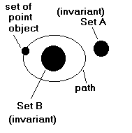
Figure 1: Circular Motion

Physically, this above situation could, as an example, represent “revolution” of the chosen point-object around the set $B$ that is at rest relative to the reference set $A$.

The Borel automorphism in question describes the “complete” trajectory of the point object in this situation and, hence, “encodes” the entire information about all the forces that are needed to determine the trajectory of the same point object in theories using the notion of force.

[Because we limit ourselves here to only a general discussion of physical issues arising in universal relativity, we shall not explicitly display the Borel automorphism corresponding to the motion described above. However, from the group properties of the automorphisms of the standard Borel space, it is easy to see that such an automorphism indeed exists.]

Clearly, this above is a consequence of the fact that the universal relativity has only the law of motion, the Borel automorphism of the space $\mathfrak{S}$, that is also the “cause” of motion in it.

Hence, as a result of the above, if some observation is explainable in any theory using the concept of force then, the same is explained in Universal Relativity by treating the involved total force(s) as corresponding transformation(s). In this way, Universal Theory of Relativity incorporates theories that use the concept of force.

Essentially, a point object is a well-defined, non-singular, notion in the mathematical framework of Universal Relativity. If certain observation related to a physical body is “explainable” by representing the involved material body as a point particle whose motion is describable by assuming a total force (equivalently, potential field) then, in universal relativity, the same “total force” is a Borel automorphism of the space $\mathfrak{S}$ acting on the the $\Upsilon$-set of the imagined point particle.

Of course, we can adopt this above procedure of “realizing” a Borel automorphism of space $\mathfrak{S}$ for only the cases which are “explainable” by theories using the concept of force. This then also means that there will be situations in Universal Relativity which will not be explainable by theories using the concept of force.

As a consequence of the above, experimental situations can arise for which Universal Relativity can be tested in the laboratory.

Experimental tests of the Universal Theory of Relativity will then have to be developed keeping in mind this above. Specifically, we should then look for or devise experimental situations for which no “natural” explanations are offered by theories using the concept of force .

One such possibility is provided by the torsion balance experiment that has been the basis of many important experimental results related to gravity krishnan . Therefore, as an example of the situations that can arise in Universal Relativity, we discuss below the “explanations” for the outcomes of the torsion balance experiment.

The Torsion Balance Test

Consider a torsion balance consisting of a thin wire, hanging from one end at the roof, to which a dumbbell is hanging from its exact middle at the other end of the wire. Let the masses of the dumbbell be $m_{1}$ and $m_{2}$, $m_{1}=m_{2}=m$.

Next, consider “external” masses $m_{3}$ and $m_{4}$, $m_{3}=m_{4}=M$, attached to the ground, $m_{3}$ placed on one side and $m_{4}$ on another side of the dumbbell, with common center at the wire.

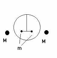
Figure 2: Torsion Balance

As per Newton’s theory, there are two possible situations in which no torque acts on the dumbbell of this assembly. The two such arrangements of the masses are: 1] the external masses and the dumbbell masses in one line and 2] line of the external masses being perpendicular to the dumbbell. Then let the dumbbell be in its natural equilibrium position in one of these states.

In Newton’s theory, “gravitational forces” are supposed to act between the “external” masses and the masses of the dumbbell, and these forces “cause” the balance to “torque” when the “external masses” are shifted, say, from the situation 1] to the situation 2]. This holds irrespective of other “couplings” of the masses, but these couplings can nullify the “gravitational” torque. Therefore, we then require and arrange that these other possible couplings have been suitably eliminated or minimized to adequate levels from the torsion balance assembly of the above type.

Consequently, in Newton’s theory, the balance will always be set into “oscillations” when the positions of the external masses are alternated between situations 1] and 2] above, say, by rotating the external masses $m_{3}$ and $m_{4}$ about the common center with the dumbbell.

In Universal Relativity, the balance setting into oscillations is “explainable” by treating the involved newtonian forces as corresponding transformations acting on the space $\mathfrak{S}$.

But, as per Universal Relativity, we also have a transformation of the “external masses” from the situation 1] to the situation 2] without the balance ever getting torqued or set into oscillations. Universal Theory of Relativity therefore also predicts that a “null outcome” is permissible for the experiment of the above type.

Let us imagine a spherical shell whose outer surface is as “frictionless” as permissible. The torsion balance is situated “inside” the spherical shell while the “external masses” are situated outside the spherical shell. [The reason why spherical shell is mentioned here is, evidently, due to its being an “invariant” of the rotation map.]

Then, the motion of external masses can be such as to not affect the interior of the spherical shell and, hence, not affecting the state of the torsion balance located inside it.

To see this above, let us first note that the torsion balance is a compound object, to be referred to as object 1, in the sense described earlier. The external masses, together, are to be considered also a compound object, object 2.

In our aforementioned experiment, we consider that the “assembly” of the torsion balance and the external masses is in one of the two “no torque states” above at the beginning of the experiment. Let $T_{i}$ be the (initial) transformation acting on the assembly of object 1 and object 2, above, ie, let the assembly be acted upon by an initial Borel automorphism $T_{i}$ of the space $\mathfrak{S}$. The nature of the initial Borel automorphism, although quite complicated, may be left unspecified in our present considerations.

Let $T_{r}$ be the transformation of the rotational motion of only the external masses and leaving the torsion balance unaffected or the corresponding $\Upsilon$-sets invariant. That is, the map $T_{r}$ acts on only the “external masses or world” to produce their rotational motion.

The transformation acting on the assembly is then the mathematical composition $T_{r}\circ T_{i}$ and its action is such that only the external masses or world external to balance revolve around the torsion balance with the $\Upsilon$-set of balance being an invariant set of the composition $T_{r}\circ T_{i}$.

Clearly, such a transformation is possible when the external masses are sufficiently away from the dumbbell masses so that the effects of rotational motion of the external masses take time to “propagate” to the dumbbell masses or when the dumbbell is well-shielded from all possible effects of the rotational motion of external masses. Universal Theory of Relativity then “guarantees” that the torsion balance will not be torqued by the motion of the external masses in the experimental situation imagined above.

Evidently, no “explicit calculations” using transformations $T_{i}$ and $T_{r}$ are needed to reach this conclusion. Universal Relativity always predicts a “complete null effect” in this situation.

If, for the same experiment, we make the external masses move not along a circle but along an elliptical orbit, there is to be no change in the conclusion of Universal Relativity which predicts a complete null effect even in this latter situation. Highly eccentric elliptic orbit for external masses would imply “enhancement” of the newtonian non-null effect. An elliptical orbit for the external masses could then be preferred over the circular orbit for obvious reasons.

Then, in certain situations, the effect on torsion balance is expected in Universal Relativity to be “total null” if shielding of the balance is proper. Then, if the external masses “rotate” around the dumbbell masses sufficiently slowly, say, one revolution in few minutes, and if we run the experiment for a couple of weeks or months, so as to obtain good statistic, we can test the Universal Theory of Relativity. Of course, this test can only be considered successful if the “null result” is observed. Else, in universal relativity, we shall be forced to conclude that the “isolation” of the torsion balance is not achieved.

Thus, if a torsion-balance experiment is sufficiently carefully performed in the aforementioned manner, we should be able to verify the possible “null effect” prediction of the Universal Theory of Relativity against that of the “certainly non-null effect” of Newton’s theory.

We then note that certain, extremely high precision, torsion balance experiments are in use . Any of these torsion balance assemblies can then be employed to verify the “null effect” predicted by the Universal Theory of Relativity.

IV Concluding Remarks

Arthur Schopenhauer:
m

$\clubsuit$ All truth passes through three stages: First, it is ridiculed. Second, it is vehemently opposed. Third, it is accepted as being self-evident. $\clubsuit$
m

Over the centuries, some fundamental concepts that led Newton to his theory acquired the status of being self-evident. Specifically, Newton’s concept of force is embedded so deep into our thinking that we treat it as a self-evident concept. No doubt, force is a very useful concept. But, while adopting this concept, we are certainly required to attribute to physical matter source properties that generate the forces in question.

However, we then choose to ignore one fundamental limitation of this conception that the source properties so attributed to physical matter cannot find any explanations with the theory that uses the (newtonian) concept of force.

Developments in Physics that took place over the times since Newton formulated his mechanics were, explicitly or implicitly, based on the concept of force, developments in Quantum Theory not being any exceptional.

[The concept of potential energy is a “byproduct” of the newtonian concept of force. From the very beginning, quantum theory “assumed” this conception of potential energy to formulate its various (Heisenberg) operators.]

Except, perhaps, for Hertz’s attempt schlipp [p. 31] when he felt the need to replace the concept of potential energy by some suitable other, no one attempted to generalize the concept of force; such strong and gripping had been the influence of Newton’s thinking on the physicists.

In his attempts to incorporate the phenomenon of gravitation within the overall framework of the theory of relativity, Einstein reached the equivalence principle and, for the first time, replaced the concept of force by that of the “curvature” of the spacetime geometry.

Although Einstein replaced the concept of gravitational force by that of the curvature of spacetime geometry, his formulation of general theory of relativity did not live up to his intentions. The same conception did not work for other forces of Nature, eg, for Coulomb’s force. Consequently, Einstein’s mathematical formulation of a theory (of gravitation) based on the principle of general relativity is logically completely inappropriate.

Einstein had “realized” such problems with his formulation of general relativity. That is perhaps why he dubbed his equations of general relativity as “preliminary” equations. This obvious “failure” led him to his numerous attempts at the Unified Field Theory. Even these attempts failed.

Many others following the methods of Quantum Theory systematically developed theoretical foundations for the successful description of the micro-physical world. For this purpose, definite but ad-hoc rules of obtaining the $\Psi$-function were first adopted and the predictions checked by ingenious experimentations.

However, Einstein had, in his ways, also realized that these developments in quantum theory too were not entirely satisfactory from the perspective of some fundamental physical issues. He had, time and again, warned schlipp ; subtle us against the pitfalls of the conceptions behind these theories - his own formulation of general relativity as well as the (probabilistic) quantum theory.

Here, we systematically built on Einstein’s aforementioned intuition and replaced the newtonian concept of force with its natural generalization as a transformation of the underlying continuum. In doing so, we were led to a natural unification of the ideas of the quantum theory and those of the general principle of relativity.

The formalism we developed satisfies one of the foremost of the requirements of a genuinely universal theory of physics: that the constants of physics “arise” in it through mutual relationships of physical objects and their values cannot be changed without essentially destroying the underlying theoretical framework. It is also the Universal Theory of Relativity that is in complete agreement with the general principle of relativity.

In the last section, § III, we discussed an experimental test, the torsion balance test, of the proposed Universal Relativity. In accordance with the scientific methodology, it would then be worthwhile to let this and such tests decide whether the proposed generalization of the newtonian concept of force is really what is appropriate one to describe the workings of the physical world.