Bistable light detectors with nonlinear waveguide arrays

Abstract

Bistability induced by nonlinear Kerr effect in arrays of coupled waveguides is studied and shown to be a means to conceive light detectors that switch under excitation by a weak signal. The detector is obtained by coupling two single 1D waveguide to an array of coupled waveguides with adjusted indices and coupling. The process is understood by analytical description in the conservative and continuous case and illustrated by numerical simulations of the model with attenuation.

Introduction.

Arrays of adjacent optical dielectric waveguides coupled by power exchange between guided modes yariv kivsh-agra , have allowed to conceive devices possessing extremely rich optical properties, already at the linear level, such as anomalous refraction and diffraction pertsch .

At nonlinear level, for intensity-dependent refractive index (optical Kerr effect), these waveguide arrays become soliton generators christ-joseph , as experimentally demonstrated in eisenberg ; morandotti ; mandelik ; expe1 ; yuri ; fleisher1 ; fleisher2 . The model is a discrete nonlinear Schrödinger equation (NLS) and nonlinearity then manifests by self-modulation of an input signal (injected radiation) that propagates as a NLS discrete soliton yuri ; andrey . These systems possess also intrinsically discrete properties aceves and the geometry can be varied to manage dispersion mark .

Figure 1: Waveguide array (index profile) driven by 2 lateral waveguides of index $n_{0}>n_{1}$. The arrows symbolize the injected radiation.

A fundamental property of nonlinear systems that has not been considered in waveguides arrays is the bistability induced by nonlinearity. It is the purpose of this work to propose and study a device where bistability, and consequent switching properties, could be observed and used to conceive for instance a detector of light sensitive to extremely weak signal.

We shall make use of the possibility to drive a waveguide array, in the forbidden band gap, through directional coupling by boundary waveguides, which results in the generation of (discrete) gap solitons khomeriki , produced by nonlinear supratransmission nst , and used to conceive resonators with nonlinear eigenstates jl .

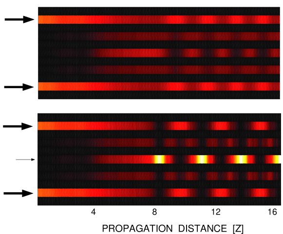
The waveguide array of figure 1, in nonlinear Kerr regime, driven by two single waveguides of index $n_{0}>n_{1}$, is operated in such a way that the guided modes in the two lateral waveguides would not linearly propagate in the array due to index difference. Nonlinear induced bistability allows then to adjust the input radiation such as to work at the bifurcation point and switch from a state of vanishing intensity output (from the central waveguides) to a state of strong intensity output, as displayed on fig.2 that represents the intensity of the flux in the array when operated close to the bifurcation point. As the switch can be operated by a very weak signal (0.03% of the input amplitude for fig.2), the device is a candidate for an ultrasensitive bistable detector.

Figure 2: (Color inline) Flux intensity along the waveguides driven at the threshold of bistability. This is the result of numerical simulations of the model (6) with $N=4$, $Q=Q_{0}=4$, $\gamma=\gamma_{0}=0.001$, $V=0.5$, and input amplitudes $b=3.0946$ (large arrows). In the lower plot the small arrow represents a signal of amplitude $0.001$ enough to trigger the switch.

After having briefly recalled the derivation of the discrete NLS model for the envelope of the guided modes and the proper boundary conditions that results from the physical context of fig.1, we describe theoretically and numerically the bistability process. The theory calls to the continuous limit which gives an accurate description of the discrete case with enough waveguides and strong coupling.

The model.

Assuming instantaneous response of the Kerr medium (of nonlinear susceptibility $\chi$) and planar wave guides along the vertical direction $x$, the electric field can be sought as $\vec{E}(\vec{r},t)=\vec{u}_{x}(E(y,z)\ e^{-i\omega t}+c.c.)/\sqrt{3\chi}$ and Maxwell’s equations reduce to

$$(\frac{\partial^{2}}{\partial y^{2}}+\frac{\partial^{2}\ }{\partial z^{2}})\ E+\frac{\omega^{2}}{c^{2}}\left(n^{2}+\mid E\mid^{2}\right)E=0,$$ (1)

where the linear index $n=n(\vec{r})$ may vary in space. Interested in the stationary regime, the fast oscillating nonlinear term has been discarded (assuming no phase matching between third harmonics).

We consider the index profile of fig.1 and assume a field component $E(y,z)$ in the form

$$E(y,z)=\epsilon\sum_{j}{\cal E}_{j}(\epsilon y)\psi_{j}(\epsilon^{2}z)e^{i\beta z},$$ (2)

where ${\cal E}_{j}$ is a guided mode, $\psi_{j}$ its amplitude and $\epsilon$ a small parameter to be defined later. The slow variation along $z$ results from the coupling between adjacent waveguides. Guided modes in both lateral waveguides, that do not propagate transversaly in the array, result from the necessary condition

$$\beta^{2}-\frac{\omega^{2}}{c^{2}}n_{0}^{2}<0,\quad\beta^{2}-\frac{\omega^{2}}{c^{2}}n_{1}^{2}>0.$$ (3)

Then, following ziad , we insert (2) in (1), integrate over $y$ and obtain the coefficients that couple the driving lateral wave guides to the array ($C_{0}$), the array waveguides together ($C_{1}$), and that result from the overlapping of modes ${\cal E}_{j}$ across the separation between waveguides. Upon defining the dimensionless variable $z^{\prime}=z\,\omega^{2}/(2\beta c^{2})$ the coupling coefficients are scaled by

$$Q=\frac{c^{2}}{\omega^{2}}C_{1},\quad Q_{0}=\frac{c^{2}}{\omega^{2}}\frac{C_{0}^{2}}{C_{1}}.$$ (4)

and we define the essential constant

$$V=n_{0}^{2}-n_{1}^{2}-2Q,\quad V>0,\quad V\sim\epsilon^{2}.$$ (5)

This defines the small parameter $\epsilon$ used in expansion (2), and provides the necessary and sufficient condition ($V>0$) for evanaescent waves along transverse direction in the array.

We obtain eventually the model (forgetting the prime on $z$ and setting $\epsilon=1$ to go back to physical units)

$$i(\partial_{z}+\gamma_{0})\psi_{0}=Q_{0}\psi_{1},\quad i(\partial_{z}+\gamma_{0})\psi_{N}=Q_{0}\psi_{N-1}$$ (6)

$$i(\partial_{z}+\gamma)\psi_{j}+Q\left(\psi_{j-1}+\psi_{j+1}-2\psi_{j}\right)+|\psi_{j}|^{2}\psi_{j}=V\psi_{j},$$

where $j$ runs from $j=1$ to $j=N-1$. Attenuation has been included (imaginary parts $\gamma$ and $\gamma_{0}$ of the dielectric constants) to account for a realistic physical situation, and the actual amplitudes in the lateral driving waveguide have been rescaled by replacing $C_{0}\psi_{0,N}$ by $C_{1}\psi_{0,N}$.

Prescription of the injected energy flux in the lateral waveguides results in defining the amplitudes $\psi_{0}$ and $\psi_{N}$ in $z=0$ (say $b$), which are associated to a set of vanishing $\psi_{j}(0)$ for the rest of the array. The initial condition is thus

$$\psi_{0}(0)=\psi_{N}(0)=b,\quad\psi_{j}(0)=0,\quad j=1\cdots N-1$$ (7)

which complete equations (6). The point is that nonlinearity causes the existence of a threshold $b_{s}$ allowing to take advantage of bistabilility of stationary states, as described now analytically and numerically.

Analytic description.

The continuous limit of (6) is obtained for

$$y=j\sqrt{1/Q},\quad\psi_{j}(z)=\psi(y,z),$$ (8)

(note that this dimension $y$ is not the physical dimension $y$ of expression (2)) and reads (without attenuation)

$$i\psi_{z}+\psi_{yy}+|\psi|^{2}\,\psi=V\psi.$$ (9)

The boundary data that represent the injected flux are taken as constants, namely

$$\psi(0,z)=\psi(L,z)=b,$$ (10)

As far as the light tunnels from the driving waveguides to the array, the amplitude of light in the driving waveguides decays along $z$. However, if the coupling $Q_{0}$ and the attenuation $\gamma_{0}$ are small enough, the intensities in the driving waveguides decay slowly along $z$ and the above boundary-value problem quite correctly matches numerical simulation of the discrete model (6).

The stationary solutions of the above problem are obtained by assuming a real valued solution depending on $y$ only, namely $\psi(y,z)=\psi(y)$ solution of

$$\psi_{yy}+\psi^{3}=V\psi,\quad\psi(0)=\psi(L)=b.$$ (11)

From the symmetry of the above bounds, a uniformly bounded function requires that there exists $y_{0}$ such that

$$\psi_{y}(y_{0})=0,\quad\psi(y_{0})=B.$$ (12)

The values $b$ and $B$ are referred respectively to as input and output amplitudes of the field. By integrating (11) with (12), one gets

$$(\psi_{y})^{2}=\frac{1}{2}(B^{2}-\psi^{2})(\psi^{2}+B^{2}-2V).$$ (13)

This equation has solutions of different types byrd depending on the relative values of $B$ and $V$. In particular, an input value $b$ of the boundary driving can produce different output amplitudes $B$. This property holds when the input amplitude $b$ is less than a value $b_{s}$, called the supratransmission threshold, above which the boundary driving induces an instability which generates soliton emission in the array instab .

Case I: $B^{2}>2V$. The integration of (13) on $[0,L]$ produces the relation

$$b=B\cdot\rm cn[\beta L/2,k],$$ (14)

where $\rm cn[\cdot,k]$ is the cosine-amplitude Jacobi elliptic function of modulus $k$. The parameters $\beta$ and $k$ obey the relation

$$\beta^{2}=B^{2}-V,\quad k^{2}=\frac{B^{2}}{2(B^{2}-V)},$$ (15)

while the whole solution (11) has the following form

$$\psi^{I}(y)=B\cdot\rm cn\left[\beta(y-L/2),k\right].$$ (16)

Case II: $V<B^{2}<2V$. The integration of (13) gives here

$$b=B\cdot\rm dn[\beta L/2,k],$$ (17)

$$\beta^{2}=\frac{B^{2}}{2},\quad k^{2}=\frac{2(B^{2}-V)}{B^{2}},$$ (18)

$$\psi^{II}(y)=B\cdot\rm dn\left[\beta(y-L/2),k\right].$$ (19)

Case III: $B^{2}<V$. In this case we obtain

$$b=\frac{B}{\rm dn[\beta L/2,k]},$$ (20)

$$\beta^{2}=\frac{2V-B^{2}}{2},\quad k^{2}=\frac{2(V-B^{2})}{2V-B^{2}},$$ (21)

$$\psi^{III}(y)=\frac{B}{\rm dn\left[\beta(y-L/2),k\right]}.$$ (22)

This last solution has a threshold amplitude $b=b_{s}$ reached when the function $b(B)$ in (20) has a vanishing derivative. The related expression of $b_{s}$ is not explicit although easily evaluated numerically. Note that in general one has a finite set of thresholds (their number depend on the lenght $L$) but only the first one is of interest for our purpose. Note also that the above three solutions reach their maximum amplitude $B$ in the array center $y=L/2$.

Bistable behavior.

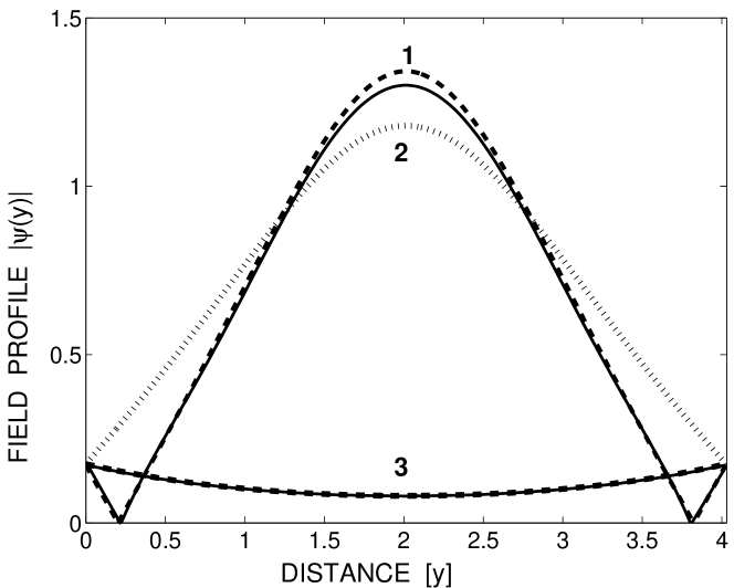
The numerical simulations of system (6), now compared to the above analytical solutions, are performed with $N=18$, $Q=20$, $Q_{0}=0.05$ and $V=0.5$. The system locks to a stationary solution thanks to the attenuation factors $\gamma=0.02$ and $\gamma_{0}=0.002$. In order to avoid an initial shock, the coupling $Q_{0}$ is actually smoothly set by using $Q_{0}(1-e^{-z/5})$. The input-output dependence resulting from of (14), (17) and (20) is plotted on fig.3 and the profiles of the different exact solutions (16), (19) and (22) corresponding to the different output amplitudes are presented in fig.4.

Figure 3: Hysteresis loop for the input-output amplitude values obtained from the analytical solutions of type I (14), II (17) and III (20) respectively. Crosses are the results of numerical simulations. The dashed vertical line represents the value of the supratransmission threshold $b_{s}$, and ther two dashed lines set upper and lower limits for the appearance of type II solution. Crossing of the full vertical line with the hysteretic curve defines input-output values 1, 2 and 3 chosen for fig.4.

Figure 4: Analytic solutions (dashed lines) corresponding to the single input amplitude $b=0.18$ compared to numerical experiments (solid lines).

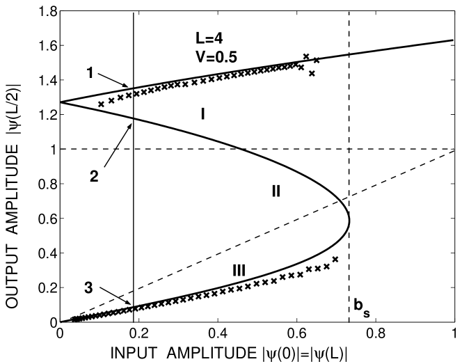
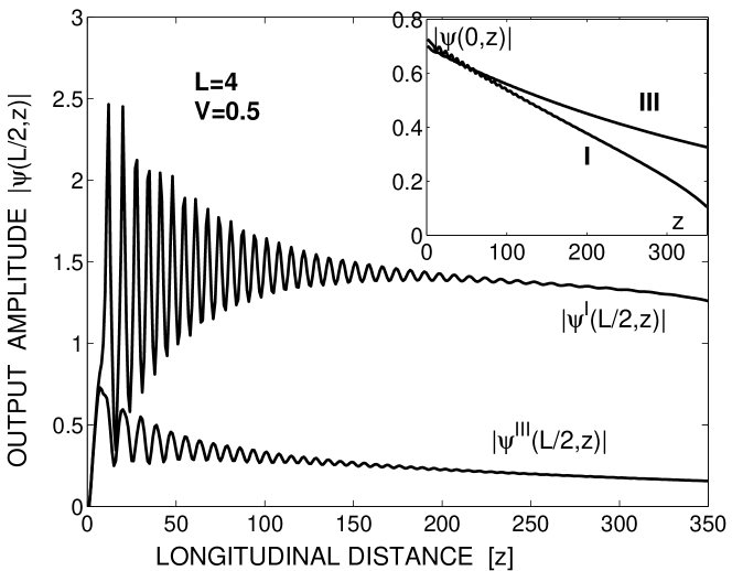
The regimes of stationary solutions are reached by numerical simulations of (6) as follows. First we inject into the driving waveguides the beams with the initial amplitude (7) for $b<b_{s}$. This produces the type III solution, a nonlinear analogue to the evanescent wave profile. As the amplitudes $|\psi_{0}(z)|$ and $|\psi_{N}(z)|$ in the driving waveguides decay along $z$ we monitor the amplitude $|\psi_{N/2}(z)|$ at the middle of the array as a function of the driving amplitudes. At some distance $z_{0}$ from the origin, the system stabilizes to a stationary profile (as shown by fig.5) and we measure there the corresponding amplitudes $B=|\psi_{N/2}(z_{0})|$ and $b=|\psi_{0}(z_{0})|$, plotted then as the crosses along the lower branch (III) in fig.3. (Note that only the solutions of type I and III can be reached by numerical simulations, while the type II is unstable and eventually decays to the stable solution III. Note also that longer lengths would allow for multiple output amplitudes, which we do not consider here.)

The same procedure is used when injecting the beams with $b>b_{s}$. After a regime of gap solitons emission, the amplitudes along the lateral waveguides decrease below the threshold $b_{s}$, allowing the system to lock to the solution of type I. The obtained numerical values are plotted (crosses) along the upper branch (I) of the hysteresis loop in fig.3.

The analytical curves slightly overestimate the numerical results because of the attenuation (optical losses in the laboratory experiments) included in our numerical simulations. Another consequence of the attenuation is the existence of a second (nonzero) threshold input amplitude where the solution bifurcates back from the regime I to the regime III. For a vanishing attenuation, this second threshold would be exactly zero according to the analytical solution (16). The existence of this lower end threshold is clearly of importance in view of experimental realization but, as being directly related to attenuation, it depends on the precise physical context. Let us also remark that the output amplitude is sensitive to the input amplitude values (in both regimes). In particular the curves (and dots) of fig.3 show that this dependence is roughly linear as the slopes of the functions $B(b)$ in regimes I and III have approximately the same slopes.

As a matter of fact we display on the fig.5 the evolution of the amplitudes $|\psi_{0}(z)|=|\psi_{N}(z)|$ along the driving waveguides and the amplitude in the middle of the array $|\psi_{N/2}(z)|$ obtained from a numerical simulation. The difference between the two output signals at $y=L/2$ in these two regimes differs substantially (approximately by two orders of magnitude).

Figure 5: Evolution of input (inset) and output (main plot) amplitudes along the propagation direction $z$. Note the difference between output amplitudes $|\psi(L/2,z)|$ in two regimes although the initial values of the amplitudes in the boundary waveguide $b$ slightly differ from each other.

The existence of bistable regimes that switch from a low to a high output is a candidate for an ultra sensitive bistable light detector. Moreover such a property holds also in the fully discrete case as displayed in fig.2 (though we do not have in that case an analytical description). Particularly, if one injects in the lateral waveguides beams of amplitude slightly below the supratransmission threshold $b_{s}$, a regime of type III establishes (with small output amplitude). Then any perturbation of the array by means of a weak input signal destabilizes the system which, after transient emission of gap solitons, reaches a type I regime with large output amplitude. This is precisely the process described in the intensity plot of fig.2 where the signal producing the switch carries 0.03% of the driving amplitude.

Note that in such a fully discrete case, the device works as a digital detector, triggered by any signal received by the central waveguides. However in the continuous case, the output signal amplitude can be (approximately) linearly related to the input amplitude and, if the variable parameter is the input amplitudes in the lateral waveguides, then the device can be operated as an amplificator.

Acknowledgements: R. Kh. acknowledges financial support from NATO and thanks International Centre for Theoretical Physics (Trieste, Italy) for the hospitality.

References

- (1) A. Yariv, Optical Electronics, Saunders College Pub. fourth ed., Orlando FL (1991)
- (2) Y.S. Kivshar, G.P. Agrawall, Optical Solitons: From Fibers to Photonic Crystals, Academic Press, San Diego, CA (2003)
- (3) T. Pertsch, T. Zentgraf, U. Peschel, A. Brauer, F. Lederer, Phys Rev Lett 88 (2002) 093901
- (4) D.N. Christodoulides, R.I. Joseph, Optics Lett 13 (1988) 794
- (5) H.S. Eisenberg, Y. Silberberg, R. Morandotti, A.R. Boyd, J.S. Aitchison, Phys Rev Lett 81 (1998) 3383
- (6) R. Morandotti, H.S. Eisenberg, Y. Silberberg, M. Sorel, J.S. Aitchison, Phys Rev Lett 86 (2001) 3296
- (7) D. Mandelik, H.S. Eisenberg, Y. Silberberg, R. Morandotti, J.S. Aitchison, Phys Rev Lett 90 (2003) 053902
- (8) D. Mandelik, R. Morandotti, J.S. Aitchison, Y. Silberberg, Phys Rev Lett 92 (2004) 093904
- (9) A.A. Sukhorukov, D. Neshev, W. Krolikowski, Y.S. Kivshar, Phys Rev Lett 92 (2004) 093901
- (10) J.W. Fleischer et al., Phys Rev Lett 90 (2003) 023902
- (11) J.W. Fleischer et al., Nature 422 (2003) 147
- (12) A.A. Sukhorukov, Y.S. Kivshar, Phys Rev E 65 (2002) 036609
- (13) A.B. Aceves, C. De Angelis, T. Peschel, R. Muschall, F. Lederer, S. Trillo, S. Wabnitz, Phys Rev E 53 (1996) 1172
- (14) M.J. Ablowitz, Z.H. Musslimani, Phys Rev Lett 87 (2001) 254102; and Phys Rev E 65 (2002) 056618
- (15) N. K. Efremidis, D. N. Christodoulides, Phys Rev E 65 (2002) 056607
- (16) R. Khomeriki, Phys Rev Lett 92 (2004) 063905
- (17) F. Geniet, J. Leon, Phys Rev Lett 89 (2002) 134102; and J Phys Cond Matt 15 (2003) 2933
- (18) J. Leon, Phys Rev E 70 (2004) 056604
- (19) M.J. Ablowitz and Z.H. Musslimani, Physica D 184 (2003) 276
- (20) P.F. Byrd, M.D. Friedman, Handbook of elliptic integrals for engineers and physicists, Springer (Berlin 1954)
- (21) J. Leon, Phys Lett A 319 (2003) 130