Elliptically Symmetric Polarized Beams

Abstract

We study the free-propagation features of an optical field endowed with a non-uniform polarization pattern with elliptical symmetry. The fields derived in this way are called Elliptically Symmetric Polarized Beams (ESPB for short). Some properties of those fields are analysed. Moreover, it is shown how it is possible to obtain such light beams by applying the result to Bessel-Gauss beams.

1 Introduction

Recently there was a growing interest, in the Optics community, towards those optical fields possessing unusual polarization features; this because some phenomena have shown to be strongly dependent by vectorial properties of the field. For instance, it was experimentally demonstrated that a radially polarized field can be focused to spot size of extension much smaller than that obtainable by using a linear polarized one [1]. Also, azimuthally and radially polarized fields [2] have found use in many sector of Optics, like particle beam trapping, optical microscopy, superrisolution [3], specially when those polarization features are associated to a particular intensity profile (the so-called donut beams are an example of that) which implies the presence of a strong longitudinal component of the optical electric field; moreover it was shown that beams possessing field lines in the shape of a spiral, namely spirally polarized beams, are suitable to describe fields with vortices in their transverse phase profile [4]. In the present paper we wish to widen this scenario, by introducing coherent beams with a non-uniform polarization state with an elliptical symmetry. By doing so, we wish to show how some of aforesaid properties are easily extendable to other polarization’s geometry and to emphasize the differences among all those polarizations. The paper is organized as follows: in section 2, after having recalled briefly some definitions about cylindrical coordinate system, we specialize the subject to elliptical symmetry; in section 3 we derive some results in paraxial optics regime by applying the theory to Bessel-Gauss beams.

2 Field and polarization symmetries

Let us suppose we have a free-space beam, which propagates along a mean direction, say $z$-axis, on starting from a source-plane on which we know the field distribution of amplitude and phase. In this context the term non-uniform, when addressed to the field polarization features, implicity refers to the transverse component of the field analysed through a rectangular (Cartesian) coordinate system. So we say that a polarization is non-uniform if, on moving along a fixed direction in the $(x,y)$ plane, we see the vector field changing in direction when compared with the unit vector basis ${\hat{x}}$ and ${\hat{y}}$. In reality, it should be still possible to find a new coordinate system respect to which the field mantains its polarization state. In other words, the field should be uniformly polarized respect to this new coordinate system. In a generical cylindrical orthogonal reference frame we can write the field, across the plane $z=0$, as

$${\bf E}={\bf E_{T}}+E_{z}\hat{z}$$ (1)

where

$${\bf E_{T}}(q_{1},q_{2},0)=E_{1}(q_{1},q_{2},0){\hat{q}_{1}}+E_{2}(q_{1},q_{2},0){\hat{q}_{2}}$$ (2)

indicates the trasverse field and ${\hat{q}_{1}}$, ${\hat{q}_{2}}$ and $z$ indicate the vector basis of a generical cylindrical orthogonal coordinate system, which is related to a Cartesian orthogonal system by the following relationships

$$x=g_{1}(q_{1},q_{2})$$

$$y=g_{2}(q_{1},q_{2})$$ (3)

$$z=z$$

where $g_{1}$ and $g_{2}$ are smooth functions of $q_{1}$, $q_{2}$ variables. Rectangular and circular ones are special cases of equations (2). In particular, speaking about circular symmetry, recently several authors have focused their attention on fields polarized in a radially or azimuthally way. In almost all these works also the field (i.e the amplitude and phase of each scalar component of the optical field, and not only the polarization) was choosen to be circularly simmetric. While this choice seems to be the most obvious and natural, anyhow it can be interesting to study the case in which this coupling in symmetry is removed, a case that does not have received attention at all. This fact is a little odd, specially if one thinks to the way in which a radially or azimuthally circular polarized field can be obtained in practice [5]. For instance, one of the methods to obtain a radially polarized beam is to combine coherently an Hermite-Gauss beam of order $(0,1)$ and an analogous beam, but of order $(1,0)$, both arising from a laser beam, on supposing that amplitude and phase of the two beams are the same. There exist other metods, but all of them also suppose to have a very good control of the amplitude of the two component that one adds togheter. Actually this is true only approximately and in practice one can consider the effect of some difference in amplitude between the two emerging beams, a difference which gives rise just to an elliptical symmetry. In the next section we start by analysing the form of a generical field endowed with features that break both the circular than rectangular symmetry and we will discuss the relative properties.

2.1 Vectorial beam with elliptical symmetry

Let us suppose we have a field like that in equation (1) and ${\bf E_{T}}$ be

$${\bf E_{T}}=Af(r,z)\cos(\theta+\alpha){\hat{x}}+Bf(r,z)\sin(\theta+\alpha){\hat{y}}$$ (4)

where $A$ and $B$ indicate two arbitrary real constants, $r$ and $\theta$ are, respectively, the radial and angular coordinates of a circular-symmetric coordinate system, $f(r,z)$ is a radial-circular function across a $z$ plane and $\alpha$ is a constant angle. We suppose here that $A\neq B$. It is straightforward to show that the field in equation (4) can be rewritten as follows

$${\bf E_{T}}=Cf(r,z)[\sinh\xi\cos(\theta+\alpha){\hat{x}}+\cosh\xi\sin(\theta+\alpha){\hat{y}}]$$ (5)

by choosing the terms $C$ and $\xi$ as

$$C^{2}=B^{2}-A^{2}$$ (6)

$$\cosh\xi=\frac{B}{C}$$ (7)

The first observation we do is trivial. If we fix the radial coordinate and we let to vary only $\theta$-variable, we will see the arrow describing the electric field in equation (4) to describe an ellipse with semiaxis $Af(r,z)$ and $Bf(r,z)$. More interesting is to find the shape of the field lines for the aforesaid field. To achieve this goal we prefer to refer to a circular coordinate system. To obtain the field lines one needs to solve the equation

$${\frac{dy}{dx}}={\frac{E_{y}}{E_{x}}}={\frac{B\sin(\theta+\alpha)}{A\cos(\theta+\alpha)}}$$ (8)

which becomes, in polar coodinates,

$${\frac{\sin\theta dr+r\cos\theta d\theta}{\cos\theta dr-r\sin\theta d\theta}}=a{\frac{\sin\theta\cos\alpha+\cos\theta\sin\alpha}{\cos\theta\cos\alpha-\sin\theta\sin\alpha}}$$ (9)

where we have defined a new constant $a=B/A$. Equation (9) can be transformed into the following relation

$${\frac{dr}{r}}=d\theta{\frac{[-(\cos^{2}\theta+a\sin^{2}\theta)\cos\alpha+\sin 2\theta\sin\alpha(1-a)/2]}{[\sin 2\theta\cos\alpha(1-a)/2-\sin\alpha(\sin^{2}\theta+a\cos^{2}\theta)]}}$$ (10)

by recalling the relationship between Cartesian and circular coordinates. We note that when $a=1$ (i.e in the circular-symmetric case) this equation reduces to

$${\frac{dr}{r}}=d\theta{\frac{\cos\alpha}{\sin\alpha}}$$ (11)

and the solution is a line in the shape of a logarithmic (circular) spiral [4]. Solving equation (9) is a little more difficult because the presence of the coefficient $a$ breaks the polar symmetry. We can start by studying two particular cases, i.e, when $\alpha=0$ and $\alpha=\pi/2$. In the first case ($\alpha=0$) equation (9) becomes

$${\frac{dr}{r}}=d\theta{\frac{\cos^{2}\theta+a\sin^{2}\theta}{(a-1)\sin\theta\cos\theta}}$$ (12)

This equation can be solved, by rewriting it in the following form

$${\frac{dr}{r}}=d\theta{\frac{\cos\theta}{(a-1)\sin\theta}}+{\frac{a\sin\theta}{(a-1)\cos\theta}}$$ (13)

and it gives

$$r(\theta)=R[{\frac{\sin\theta}{(\cos\theta)^{a}}}]^{1/(a-1)}$$ (14)

where $R$ is an integration constant. Equation (14) describes open lines, which tend to lines through the origin when $a\rightarrow 1$, and that represent the analogous of radial-circular polarization for the geometry in subject, namely a radial-elliptical polarization. In Cartesian coordinates it reduces to the following relation between $x$ and $y$ coordinates

$$y=Kx^{a}$$ (15)

where K is a constant value. In the other case ($\alpha=\pi/2$) equation (10) becomes

$${\frac{dr}{r}}=d\theta(a-1){\frac{\sin\theta\cos\theta}{(1+(a-1)\cos^{2}\theta}}$$ (16)

and it gives

$$r(\theta)=R{\frac{1}{(1+(a-1)\cos^{2}\theta)^{1/2}}}$$ (17)

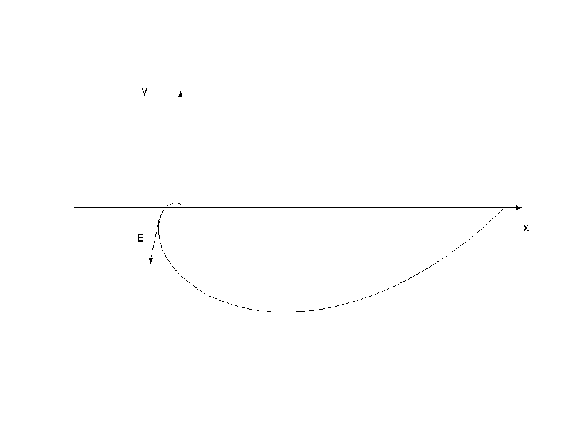
Figure 1: elliptical logarithmic spiral. The parameters are choosen as follows: $B/A=10/3$, $\alpha=0.8$.

This is the polar form of ellipses, with (on considering $a>1$) the major axis parallel to y-axis and it represents the azimuthal polarization for elliptical geometry namely an azimuthal-elliptical polarization. When $a=1$ the ellipses become circles (described by $r=R$ relation), i.e. we find again the circularly-symmetric case. For the intermediate case, that is for $\alpha\neq 0,\pi/2$, the integration of the respective differential equation is less easy. In Figure (1) we report the solution after having choosen $\alpha=0.8$ and the quotient $a=B/A=10/3$. The field line that arises is a logarithmical (but elliptical) spiral. Spirally beams were introduced by Gori [4] for circular-symmetric case and here we found a natural extension to elliptically-symmetric case. In the following we analyse some properties of this kind of beam. We have already seen which is the role of $\alpha$ angle: when it tends to zero the polarization tends to become radial-elliptical, the field being tangent to curves like in equation (15) whereas when it tends to $\infty$ the polarization tends to be azimuthal-elliptical, the field being tangent to ellipses described by equation (17). Also we note that the beam described by equation (5) is anisotrope, i.e its tranverse intensity pattern depends by $\theta$ angle. Indeed, for the intensity of transverse component holds

$$I_{T}(r,\theta,z)\propto{|\bf E_{T}|}^{2}=C^{2}|f(r,z)|^{2}[\cosh^{2}\xi-\cos^{2}(\theta+\alpha)]$$ (18)

in which the angular dependence is evident. It is simple to see that the maximum intensity directions are

$$\theta_{1}=\pi/2-\alpha\pm m\pi\\$$

($m=0,1,2..$) in which equation (18) becomes

$$I_{T}(r,\theta,z)\propto{|\bf E_{T}|}^{2}=C^{2}|f(r,z)|^{2}\cosh^{2}\xi$$ (19)

so we can find the value of angle $\alpha$ and, as a consequence, also the polarization kind, by intensity measurement, contrary to the circular-symmetric case in which the intensity is dependent only from the radial coordinate $r$ and does not give any information about polarization. In other words, in the circular-symmetric case all transverse intensity profiles associated to a particular polarization state (radial, azimuthal, spiral ones, etc.) are undistinguishable one to another. In the elliptical-symmetric case, one can obtain all the parameters, i.e. the ratio $B/A$ and the angle $\alpha$, simply by the intensity transverse map measured across a generical tranverse plane. Indeed, with reference to equation (18), by measuring the maximum intensity direction one evalues the angle $\alpha$ (equation (2.1), whereas by measuring the angular-visibility ratio

$$\nu_{r}=\frac{I_{Max}-I_{Min}}{I_{Max}}=\frac{1}{\cosh^{2}\xi}$$ (20)

one evalues the values of $A$ and $B$ (the indice $r$ indicates that the radial coordinate is fixed). Also we note that the equation (18) never goes to zero, this because the term $\cosh^{2}\xi-\cos^{2}(\theta+\alpha)$ is different to zero $\forall\xi\neq 0$ (the case $\xi=0$ represents linear polarization and here is not considered). It follows that it ever holds $\nu<1$. It remains to see how one can obtain such a field. This is the purpose of the next section.

3 Elliptically Symmetric Polarized Bessel-Gauss Beams

It is well known that Bessel-Gauss beams ($BG$ beams for short) are solution of scalar paraxial wave equation and were introduced for the first time from Gori et al. [7]. In particular Gori introduced the linearly polarized $BG$ beams of zero-order, here denoted for convenience as $BG_{0}$. Subsequently many authors have been interested both to the generalization to vectorial [9] and higher-order $BG$ beams, both to beam with unusual polarization features, as azimuthal and radial ones [6]. Here we recall, for reader convenience, the form of a $BG_{0}$

$$BG_{0}=\frac{1}{(1+iz/L)}J_{0}[\frac{\beta r}{(1+iz/L)}]\exp[\frac{-r^{2}}{w^{2}(1+iz/L)}]\exp[\frac{-i\beta^{2}z}{2k(1+iz/L)}]$$ (21)

where $J_{0}$ is the zero-order Bessel function of the first kind, $L$ is the Rayleigh length, $w$ is the minimum spot size of the Gaussian beam, and $\beta$ is the intensity of the tranverse wave vector; to extend the vectorial treatise to encompasse also a non-uniform elliptical polarization we start from a vectorial paraxial wave equation. On starting from Maxwell’s equations in vacuum, in absence of sources, we arrive to the following equation for the complete vector field $\bf E$

$$\nabla\times\nabla\times{\bf E}=k^{2}{\bf E}$$

$$\nabla\cdot{\bf E}=0$$ (22)

On introducing a ”slowly varying part” of ${\bf E}$, say ${\bf F}$, with

$${\bf E}={\bf F}\exp(ikz)$$ (23)

and by making use of the paraxial approximation, we obtain that ${\bf F}$ is governed from the following equations [10]

$$\nabla^{2}_{T}{\bf F_{T}}+2ik\partial_{z}{\bf F_{T}}=0$$ (24)

$$\nabla_{T}\cdot{\bf F_{T}}+ikF_{z}=0$$ (25)

in which we have decomposed the field ${\bf F}$ in longitudinal and transverse component, i.e. ${\bf F}={\bf F_{T}}+F_{z}\hat{z}$. Now, if we decompose also the field ${\bf F_{T}}$ into rectangular component, i.e. we let ${\bf F_{T}}=F_{x}\hat{x}+F_{y}\hat{y}$ we obtain two scalar paraxial wave equations, each for single component,

$$\nabla^{2}_{T}{F_{x}}+2ik\partial_{z}{F_{x}}=0$$ (26)

$$\nabla^{2}_{T}{F_{y}}+2ik\partial_{z}{F_{y}}=0$$ (27)

equation (26)-(27) can be rewritten as $LF_{x}=0$ and $LF_{y}=0$, after introduced a linear differential operator $L=\partial^{2}_{x}+\partial^{2}_{y}+2ik\partial_{z}$. Now, as the $L$ operator commutes with the infinitesimal displacement operators [8] $\partial_{x}$, $\partial_{y}$ and $\partial_{z}$, it is possible to obtain new solutions from known solutions by mean of arbitrary differentiation. This observation will be crucial to obtain elliptically symmetric polarized $BG$ beams. Indeed, the first thing to do is differentiating, respect to $x$ and $y$ variables, a $BG_{0}$ beam; in this way we obtain two new possible solutions for a scalar paraxial wave equation: $\partial_{x}BG_{0}$ and $\partial_{y}BG_{0}$. If we now linearly combine them properly we find the ESPB. To this purpose it is sufficient to let

$$F_{x}=A[\partial_{x}(BG_{0})\cos\alpha-\partial_{y}(BG_{0})\sin\alpha]$$ (28)

$$F_{y}=B[\partial_{y}(BG_{0})\cos\alpha+\partial_{x}(BG_{0})\sin\alpha]$$ (29)

in which $A$ and $B$ are two arbitrary constant, with $A\neq B$, and $\alpha$, as usual, is a constant angle. On utilizing the position in equations (6)-(7) we finally obtain

$${\bf F_{T}}({\bf r},z) = \frac{C}{(1+iz/L)^{2}}\exp[-\frac{r^{2}}{w^{2}(1+iz/L)}]\times$$ (30)

$$\times \exp[-\frac{i\beta^{2}z}{2k(1+iz/L)}][\beta J_{1}(\frac{\beta r}{1+iz/L})+$$

$$+ \frac{2r}{w^{2}}J_{0}(\frac{\beta r}{1+iz/L})][\sinh\xi\cos(\theta+\alpha)\hat{x}+\cosh\xi\sin(\theta+\alpha)\hat{y}]$$

As the paraxial propagation has to be satisfied, from equation (30) follows that the function $f(r,z)$ on the source plane ($z=0$) can’t be choosen in a arbitrary way. In particular, by comparing equation (4) and equation (30), we have

$$f(r)=f(r,z)|_{z=0}=\exp[-\frac{r^{2}}{w^{2}}][\beta J_{1}(\beta r)+\frac{2r}{w^{2}}J_{0}(\beta r)]$$ (31)

In Figures (2) we report the intensity pattern of a ESP Bessel-Gauss beam, evalued at different transverse planes. We see that the beam mantains, during its paraxial propagation, a zero in correspondence of $z$ axis (a properties that is shared with the classical donut beams). In Figure (3) we report the polarization pattern, in correspondence to the $z=0$ plane, in which is shown the behaviour of tranverse field for $\alpha=0.8$, and a ratio $B/A=10/3$. On changing the sign of the linear combination in equation (28) as well as the ratio $B/A$ one can obtain other interesting polarization pattern. In Figure (4) we plot intensity across the tranverse plane $z=0$, for different values of angle $\alpha$, to show the aforesaid angular dependence. Before closing the present section, we wish to say something about the longitudinal component of the electric field. To do that we will refer to the generical form of EPSB as that in equation (5) and we shall use equation (25) to obtain the longitudinal component in paraxial regime:

$$F_{z}=\frac{i}{k}\nabla_{T}\cdot{\bf F_{T}}$$ (32)

After straightforward calculations we find

$$F_{z} = (\partial_{r}{f(r,z)}+\frac{f(r,z)}{r})\sinh\xi\cos\alpha+\exp(-\xi)[(\partial_{r}{f(r,z)}\sin^{2}\theta+$$

$$+ \frac{f(r,z)}{r}\cos^{2}\theta)\cos\alpha+\frac{1}{2}(\partial_{r}{f(r,z)}-\frac{f(r,z)}{r})\sin\alpha\sin 2\theta]$$

which represents the full form of the longitutinal component in paraxial approximation. Here we see that, contrary to the circular-symmetric case for which an azimuthally polarized field does not give rise to a component along the z-axis, when we have an azimuthal-elliptical polarization (for which $\alpha=\pi/2$), $F_{z}$ is not null and holds

$$F_{z}=\exp(-\xi)[\frac{1}{2}(\partial_{r}{f(r,z)}-\frac{f(r,z)}{r})\sin 2\theta]$$ (34)

and it goes to zero as $\exp(-\xi)$. This is obvious if we recall that when $\xi\rightarrow\infty$ the geometry polarization tends to become circular because for high value of $\xi$, $\sinh\xi\approx\cosh\xi\approx\exp(\xi)$ and the ellipses in equation (17) tend to become circles. The fact that the longitudinal component changes by changing coordinate system is well-known and it can explained by mean a geometrical point of view. Indeed, equation (32) states that ${F_{z}}$ is a divergence of a vectorial field. The divergence $\nabla_{T}\cdot{\bf F_{T}}$ counts the algebrical sum of sinks (i.e. where a field line of ${\bf F_{T}}$ terminates) and sources (i.e. where a field line of ${\bf F_{T}}$ originates) into a surface element, across a $(x,y)$ plane. Since the divergence is a pseudoscalar, namely we are dealing with a density, it is not invariant under a generical space deformation. If, for example, the space is squeezed in a way in which the areas are reduced, the density (i.e. $F_{z}$) increases. In practice, a distortion of space can be thought as a transformation of coordinates and the fact that the divergence operation is dependent by the coordinate system in which we work means that we are dealing with metrical, and not topological, features of the field [11].

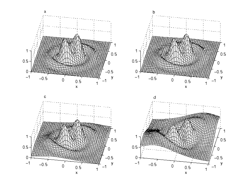
Figure 2: Tranverse intensity of a ESP Bessel-Gauss beam with non-uniform elliptical polarization at different $(x,y)$ plane. a) $z=0$; b)$z=0.1L$;3)$z=0.2L$;4)$z=0.3L$, where $L$ is Rayleigh length. The intensity is normalized at one to each plane. With reference to equation(30), we have $\beta=8/w$, $\alpha=0.8$, $B/A=2$. The axises are normalized to $w$ value.

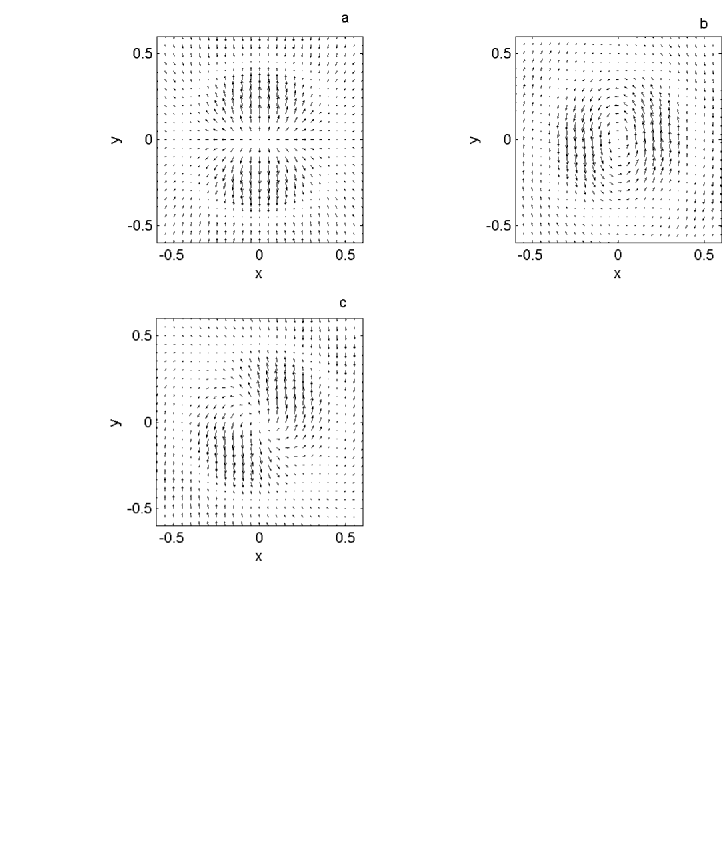
Figure 3: Polarization pattern of a ESP Bessel-Gauss beam across source plane ($z=0$). The parameters are choosen as follows: $B/A=10/3$,$\beta=8/w$ and a)$\alpha=0$, b)$\alpha=\pi/2$, c)$\alpha=0.8$. The axises are normalized to $w$ value.

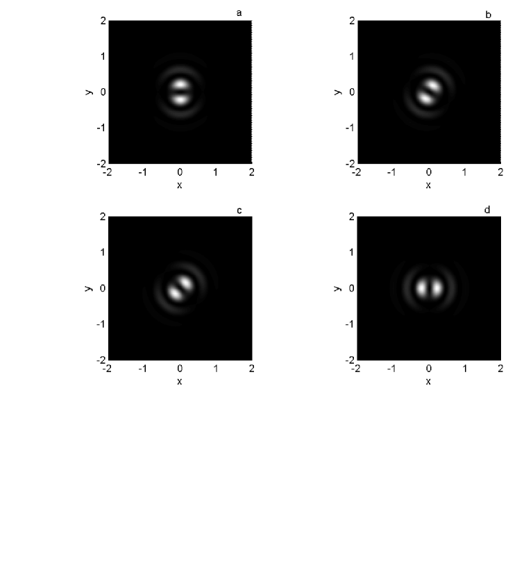
Figure 4: Intensity map of a ESP Bessel-Gauss beam across source plane ($z=0$) for different values of polarization angle $\alpha$: a) $\alpha=0$, b) $\alpha=\pi/6$ c) $\alpha=\pi/4$ d)$\alpha=\pi/2$. The parameters are choosen as follows: $B/A=10/3$,$\beta=8/w$. The axises are normalized to $w$ value.

4 Conclusion

We have introduced unconventionally polarized optical beams endowed with elliptically-symmetric features in their tranverse polarization pattern. A beam of this kind mantains its polarization state under free-space paraxial propagation. In particular we have derived a natural extension to elliptically-symmetric case of spirally-polarized beams introduced by Gori [4] for circular symmetric case. Some properties of this kind of field have been analysed. In particular, we have pointed out that, by using an elliptically-symmetric polarization, the tranverse intensity profile gives directly information about the polarization state, the angular behaviour of the intensity depending from it. This implies that it is possible to measure the field polarization state only by an acquisition of the intensity pattern across a generical tranverse plane. This is in contrast with the analogous situation in circular-symmetric case, in which the intensity pattern is indipendent from the particular polarization state. Indeed, a field polarized in a radially way produces a tranverse intensity profile identical to that produced by the azimuthally or spirally polarized ones, or any other combination of them which mantains the circular symmetry. Due to its important role in optics microscopy, we have reported also the form of the longitudinal component for the electric field, in paraxial approximation.

5 Acknowledgement

The author wishes to thank Massimo Santarsiero for useful discussions and suggestions about the subject of the present work.

References

- [1] R.Dorn, S. Quabis and G. Leuchs, Phys. Rev. Lett. 91, 233901 (2003)
- [2] As it will be more clear in the following, it would be more correct to refer to such polarization feature as azimuthal-circular and radial-circular one in order that one can put into evidence the coordinate system to which they refer.
- [3] L.Novotny, M. R. Beversluis, K. S. Youngworth, and T. G. Brown, Phys. Rev. Lett. 86, 5251 -5254 (2001);
- [4] F. Gori,J. Opt. Soc. Am. A 18, 1612-1617 (2001).
- [5] S. C. Tidwell, D. H. Ford and W. D. Kimura,Appl. Opt. 29, 2234-2239 (1990).
- [6] R. H. Jordan and G. D. Hall, Opt. Lett. 19, 427-429 (1994).
- [7] F. Gori, G. Guattari and C. Padovani, Opt. Commun. 64, 491-495 (1987).
- [8] A. Wunsche, J. Opt. Soc. Am. A, 8, 1320-1329 (1989).
- [9] P. L. Greene and D. G. Hall,J. Opt. Soc. Am. A 15, 3020-3027 (1998)
- [10] R. Borghi, M. Santarsiero, J. Opt. Soc. Am. A 21, 2029-2037 (2004).
- [11] G. Weinreich, Geometrical Vectors, (The University of Chicago Press, Chicago, US,1998, 60-61)