Optimal control in large open quantum systems –
the case of transmon readout and reset

Abstract

We present a framework that combines the adjoint state method together with reverse-time back-propagation to solve otherwise prohibitively large open-system quantum control problems. Our approach enables the optimization of arbitrary cost functions with fully general controls applied on large open quantum systems described by a Lindblad master equation. It is scalable, computationally efficient, and has a low memory footprint. We apply this framework to optimize two inherently dissipative operations in superconducting qubits which lag behind in terms of fidelity and duration compared to other unitary operations: the dispersive readout and all-microwave reset of a transmon qubit. Our results show that, given a fixed set of system parameters, shaping the control pulses can yield 2x improvements in the fidelity and duration for both of these operations compared to standard strategies. Our approach can readily be applied to optimize quantum controls in a vast range of applications such as reservoir engineering, autonomous quantum error correction, and leakage-reduction units.

Introduction.—

Quantum optimal control (QOC) provides a framework to design external controls for realizing arbitrary quantum operations with maximal fidelity and minimal time [1, 2, 3], crucial requirements of useful quantum error correction [4]. In most practical QOC applications, like the preparation of complex quantum states [5, 6, 7], or the design of fast, high-fidelity quantum gates [8, 9, 10, 11], only closed-system quantum dynamics are considered. This simplification relies on the assumption that minimizing operation time will also reduce the impact of environmental noise. However, these approaches are limited by the fact that controlling the system’s coherent dynamics can drastically alter the impact of some noise sources, as exemplified by dynamical decoupling methods [12, 13, 14]. Moreover, closed-system approaches cannot extend to inherently dissipative processes such as qubit readout and reset. Consequently, optimally controlling open quantum systems emerges as an important avenue [15, 16]. It addresses both the minimization of decoherence in quantum information processing [17, 18, 19] and the design of dissipative protocols [20, 21], marking a significant step towards comprehensive quantum control in engineered systems.

Over the last decade, several approaches have emerged for open-system QOC. Methods like Krotov [22] and gradient-ascent pulse engineering (GRAPE) [23, 24] were generalized to include dissipation [21, 25] but stay limited to unitary problems. Closed-loop control methods based on feedback engineering [26, 27] or reinforcement learning [28, 29, 30, 31] have seen recent success but fall short in scaling to large numbers of parameters. Automatic differentiation [32, 33, 34, 35] fulfills most QOC framework requirements, but suffers from substantial memory demands even for moderate system sizes and evolution times [36].

In this Letter, we present a framework enabling the realization of QOC on large open quantum systems with a fully general parametrization over the controls and arbitrarily complex cost functions. Our approach combines the adjoint state method [37, 38, 39] with reverse-time back-propagation [40, 41, 42, 43, 44] to solve otherwise prohibitive open-system quantum control problems defined in Lindblad form. This approach ensures precise and fast numerical computation of arbitrary gradients with minimal memory usage, making it ideal for GPU acceleration. In the second part of this work, we demonstrate the usefulness of this approach by optimizing two critical operations for the realization of a fault-tolerant quantum computer based on superconducting circuits: dispersive readout [45, 46, 47] and all-microwave reset [48, 49] of a transmon qubit [50].

Adjoint state method.—

Consider a QOC problem for which we seek to find a set of parameters minimizing a cost function $C(\theta,\hat{\rho}(t_{0}),\ldots,\hat{\rho}(t_{n}))$. This function, in general, depends on both the problem parameters $\theta=(\theta_{1},\ldots,\theta_{m})$ and on the density matrix of the system at a set of times, $\hat{\rho}(t_{i})$. Gradient-based approaches to optimize the control parameters rely on computing the derivative of the cost function with respect to each parameter, $\differential C/\differential\theta$. To do so, we apply the adjoint state method [37] to open quantum systems. In this context, the adjoint state is defined as $\hat{\phi}(t)=\differential C/\differential\hat{\rho}(t)$, and represents how a change in the density matrix at time $t$ modifies the cost function. For open quantum systems under the usual Born-Markov approximations [51], the evolution of the density matrix is governed by a Lindblad master equation ($\hbar=1$),

$$\frac{\differential\hat{\rho}}{\differential t}=\mathcal{L}\hat{\rho}\equiv-i[\hat{H},\hat{\rho}]+\sum_{k}\mathcal{D}[\hat{L}_{k}]\hat{\rho},$$ (1)

where $\hat{H}$ is the system Hamiltonian, $\hat{L}_{k}$ are jump operators, and $\mathcal{D}[\hat{L}]\hat{\rho}=\hat{L}\hat{\rho}\hat{L}^{\dagger}-\{\hat{L}^{\dagger}\hat{L},\hat{\rho}\}/2$. The adjoint state is then subject to a dual ordinary differential equation [52],

$$\frac{\differential\hat{\phi}}{\differential t}=-\mathcal{L}^{\dagger}\hat{\phi}\equiv-i[\hat{H},\hat{\phi}]-\sum_{k}\mathcal{D}^{\dagger}[\hat{L}_{k}]\hat{\phi},$$ (2)

where $\mathcal{D}^{\dagger}[\hat{L}]\hat{\phi}=\hat{L}^{\dagger}\hat{\phi}\hat{L}-\{\hat{L}^{\dagger}\hat{L},\hat{\phi}\}/2$. This equation can be integrated numerically over the time interval of interest $[t_{0},t_{n}]$ with initial condition $\hat{\phi}(t_{n})=\partial C/\partial\hat{\rho}(t_{n})$, computed analytically if a closed form is available, or directly through automatic differentiation. Notably, the overall minus sign in Eq. 2 ensures numerical stability of the integration by generating contracting dynamics in reverse time. The derivative of the cost function with respect to the problem parameters is given by

$$\frac{\differential C}{\differential\theta}=\frac{\partial C}{\partial\theta}-\int_{t_{n}}^{t_{0}}\partial_{\theta}\Tr[\hat{\phi}^{\dagger}(t)\mathcal{L}(t,\theta)\hat{\rho}(t)]\differential t\,.$$ (3)

This integral is straightforward to compute using the density matrix and adjoint state at each time $t\in[t_{0},t_{n}]$, as obtained from Eqs. 1 and 2. In particular, the partial derivative with respect to $\theta$ can be easily computed from automatic differentiation of the adjoint state equation by noting that

$$\partial_{\theta}\Tr[\hat{\phi}^{\dagger}\mathcal{L}\hat{\rho}]=-\Tr[\partial_{\theta}(\differential\hat{\phi}/\differential t)^{\dagger}\hat{\rho}],$$ (4)

which has the form of a vector-Jacobian product.

The QOC optimization is illustrated in Fig. 1 and proceeds in two steps. First, the forward pass consists in using the initial set of parameters (e.g. a sequence of discrete pulses) to numerically integrate the master equation from $t_{0}$ to $t_{n}$ while saving the density matrix at each time $t_{i}$ of interest. The cost function $C(\theta,\hat{\rho}(t_{0}),\ldots,\hat{\rho}(t_{n}))$ is then evaluated. To lower the memory footprint, the cost function can also be evaluated on the fly during the forward pass such that only a single density matrix needs to be stored. In a second step, the backward pass, both the master and adjoint equations are simultaneously integrated in reverse time, starting from $t=t_{n}$. During this process, the integral of Eq. 3 is iteratively evaluated, such as to obtain the entire gradients $\differential C/\differential\theta$ once the backpropagation is finished. Having access to the gradients of the cost function, we can now iteratively update the control parameters using standard optimization algorithms [53, 54, 55].

Figure 1: Adjoint state quantum optimal control. In the forward pass, the master equation is integrated and checkpointed for several time points (dark blue). In the backward pass, the density matrix $\hat{\rho}$ is recomputed in reverse time (light blue) together with the adjoint state $\hat{\phi}$ (green) and with the gradients (red) of the cost function $C$. When a checkpoint is reached, the density matrix is restored to its forward time trajectory, and the adjoint state updated with the corresponding cost function gradient.

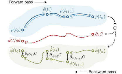
We emphasize how each density matrix (blue) is computed twice: once during the forward pass, and once during the backward pass. This enables a low memory footprint for the overall scheme, with at most a single density matrix and adjoint state needed to be stored at any given moment. The memory footprint of the method thus scales as $\mathcal{O}(N^{2})$ with $N$ the Hilbert space dimension. This is in stark contrast with methods based on automatic differentiation [33], for which the density matrix needs to be stored at each time point of the numerical integration, thus scaling as $\mathcal{O}(M_{t}N^{2})$, with $M_{t}$ the number of numerical integration steps. Such memory requirements can quickly become prohibitive, even for open quantum systems of intermediate sizes, $N\gtrsim 100$.

Note that this large gain in memory comes at the cost of trading off some numerical runtime. Overall, the scheme requires the integration of four differential equations in total [52], against only two for automatic differentiation. In addition, the reverse time integration of Eq. 1 can be numerically unstable due to the expansive dynamics of the system. This can however be fully resolved with checkpointing the quantum states during the forward pass [44], thus effectively trading back some memory for numerical stability. In practice, checkpointing at the time scale of the largest dissipation operator is sufficient to ensure numerical stability without adding significant complexity.

We have implemented this optimization scheme using PyTorch [56], taking advantage of its automatic differentiation capabilities and GPU support. This framework allows us to run optimization problems for open quantum system with hundreds of parameters, arbitrary cost functions, and for Hilbert space dimensions of up to $N\sim$5000$$ while running on a single GPU with 24 GB of memory. Our code is available through the dynamiqs open-source library [57], simplifying replication of this work and its application to various QOC problems. We now demonstrate the usefulness of this method by optimizing readout and reset of a transmon, two operations that inherently rely on dissipation.

Transmon model.—

Let us consider the experimentally realistic model depicted in Fig. 2(a) of a transmon coupled to a readout resonator and Purcell filter [58]

$$\frac{\differential\hat{\rho}}{\differential t}=-i[\hat{H},\hat{\rho}]+\gamma\mathcal{D}[\hat{b}]\hat{\rho}+\kappa\mathcal{D}[\hat{f}]\hat{\rho},$$ (5)

with transmon relaxation rate $\gamma$ and filter relaxation rate $\kappa$, and where

$$\begin{split}\hat{H}&=4E_{C}\hat{n}_{t}-E_{J}\cos(\hat{\varphi}_{t})+\omega_{r}\hat{a}^{\dagger}\hat{a}+\omega_{f}\hat{f}^{\dagger}\hat{f}\\ &-ig\hat{n}_{t}(\hat{a}-\hat{a}^{\dagger})-J(\hat{a}-\hat{a}^{\dagger})(\hat{f}-\hat{f}^{\dagger})\\ &+\Omega_{t}\hat{n}_{t}\sin(\omega_{d,t}t)-i\Omega_{f}(\hat{f}-\hat{f}^{\dagger})\sin(\omega_{d,f}t).\end{split}$$ (6)

The first two terms denote the free transmon Hamiltonian with charging energy $E_{C}$ and Josephson energy $E_{J}$, with $\hat{n}_{t}$ and $\hat{\varphi}_{t}$ the charge and phase operators, and with $\hat{b}$ the corresponding annihilation operator in the diagonal basis. The resonator and filter modes are denoted by $\hat{a}$ and $\hat{f}$, with respective frequencies $\omega_{r}$ and $\omega_{f}$. These three modes are capacitively coupled in series with coupling strengths $g\gg J$. The system can be driven using a capacitive coupling either through the transmon with a microwave pulse at frequency $\omega_{d,t}$ and envelope $\Omega_{t}(t)$, or through the Purcell filter at frequency $\omega_{d,f}$ and envelope $\Omega_{f}(t)$.

For numerical simulation of this model, we first diagonalize the free transmon Hamiltonian and identify the lowest energy eigenstates. We also diagonalize the resonator-filter subsystem yielding two normal modes, each coupled to the transmon. Finally, we apply the rotating-wave approximation (RWA) on couplings and drives. This allows for larger numerical time steps by eliminating fast oscillating dynamics thereby simplifying master equation integration. However, this also implies that not all of the chaotic or transmon ionization dynamics are captured [59, 60, 61]. To avoid probing these regimes, we limit the maximum amplitudes of control drives, e.g. to $200\text{\,}\mathrm{MHz}$ for transmon readout.

Figure 2: (a) Lumped-element model of a transmon coupled to a readout resonator and Purcell filter. The transmon and filter are driven, and the filter output field is measured through its transmission line. (b) Dispersive readout of a transmon. The mean field in the filter depends on the transmon state. Signal-to-noise ratio of readout increases with the integrated difference of mean fields. (c) Signal-to-noise ratio and assignment error of transmon readout for several drive envelopes: a flat envelope, a $4\text{\,}\mathrm{ns}$ two-step envelope [46], and optimized envelopes (QOC) with optional additional drives on the transmon at frequencies $\omega_{d,t}\simeq\omega_{r}$ (green) and $\omega_{d,t}\simeq\omega_{ef}$ (red). The flat and two-step data points are fitted according to Eq. 8. The black line shows the $T_{1}$ limit given by $\tau_{m}/2T_{1}$. (d) Reference and optimized pulse envelopes at $40\text{\,}\mathrm{ns}$ of integration time.

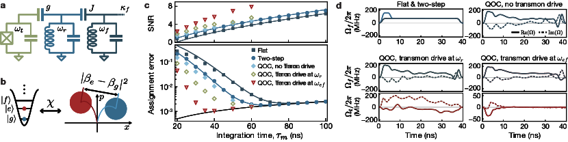
Unless stated otherwise, we use $E_{C}/2\pi=$315\text{\,}\mathrm{MHz}$$, $E_{J}/E_{C}=51$, corresponding to a bare transmon frequency $\omega_{t}/2\pi=$6\text{\,}\mathrm{GHz}$$ and to an anharmonicity $\alpha/2\pi=$-349\text{\,}\mathrm{MHz}$$. The resonator and filter frequencies are $\omega_{r}/2\pi=$7.2\text{\,}\mathrm{GHz}$$ and $\omega_{f}/2\pi=$7.21\text{\,}\mathrm{GHz}$$ with couplings $g/2\pi=$150\text{\,}\mathrm{MHz}$$ and $J/2\pi=$30\text{\,}\mathrm{MHz}$$. This yields a transmon-resonator detuning of $\Delta/2\pi=$1.2\text{\,}\mathrm{GHz}$$, a critical photon number of $\bar{n}_{\mathrm{crit}}={(\Delta/2g)}^{2}=16$ [45] and dispersive rates of $\chi/2\pi=$3.8\text{\,}\mathrm{MHz}$$ and $8.1\text{\,}\mathrm{MHz}$ with the lower and higher normal modes, respectively. Finally, the filter loss rate is $\kappa/2\pi=$30\text{\,}\mathrm{MHz}$$ and the transmon relaxation rate is $\gamma/2\pi=$8\text{\,}\mathrm{kHz}$$, i.e. $T_{1}=$20\text{\,}\mathrm{\SIUnitSymbolMicro s}$$.

Transmon readout.—

Readout of transmon qubits is realized through the dispersive coupling to a resonator [45]. In this case, the resonator frequency is shifted by the average occupancy in the transmon, and can be measured by driving the resonator at its bare frequency and monitoring the output field, see Fig. 2(b). In the presence of a Purcell filter, either normal mode of the hybridized resonator-filter subsystem can be used for readout [62].

The metric we use to maximize the measurement fidelity is the signal-to-noise ratio (SNR). Accounting for optimal weighting functions, it reads [63]

$$\mathrm{SNR}(\tau_{m})=\sqrt{2\eta\kappa\int_{0}^{\tau_{m}}\differential t\,|\beta_{e}(t)-\beta_{g}(t)|^{2}},$$ (7)

where $\eta\in[0,1]$ is the measurement efficiency, $\tau_{m}$ is the readout integration time, and $\beta_{e/g}=\Tr[\hat{f}\hat{\rho}_{g/e}\big{]}$ is the average field value in the filter mode, with $\hat{\rho}_{g/e}$ the density matrix obtained after initializing the transmon in the $\ket{g/e}$ state. To obtain results that can be compared to experiments, we use $\eta=0.6$ [46]. The optimization objective is to maximize the SNR, and thus maximize the distance between the pointer states $|\beta_{e}-\beta_{g}|$ in the shortest possible time. Further assuming that the pointer states $\beta_{g,e}$ are Gaussian, one can link the SNR and the transmon lifetime to the readout assignment error [64, 62, 52].

To optimize the transmon readout, we discretize the control pulse envelopes $\Omega(t)$ with $1\text{\,}\mathrm{ns}$ time bins and use a $250\text{\,}\mathrm{MHz}$ gaussian filter to interpolate between these pixels during numerical integration and to model realistic experimental distortions [65]. In addition to the discretized drive amplitudes, the optimization parameters $\theta$ include the carrier frequency $\omega_{d}$ of each drive. Contrary to the drive amplitudes, the latter are kept constant throughout the pulse duration, in accordance with typical experiments. The cost function used to optimize the transmon readout is principally composed of the SNR of Eq. 7, with additional cost terms constraining the control pulses in order to regularize the optimization and avoid out-of-model dynamics. For example, we limit the number of photons in the hybridized resonator-filter modes, penalize unwanted transitions to higher excited transmon states, and limit the maximal available pulse amplitudes. The full cost function is detailed in [52]. We perform gradient descent using Adam [54] and use the adjoint state method previously described to compute gradients.

Figure 2(c) shows the SNR and the assignment error as a function of the integration time $\tau_{m}$ obtained by our approach, and panel (d) shows the corresponding pulse envelopes for $\tau_{m}=$40\text{\,}\mathrm{ns}$$ optimizations. As a point of comparison, we first consider the two non-optimized reference pulses labelled ‘flat’ and ‘two-step’. The former consists of a constant pulse with $2\text{\,}\mathrm{ns}$ ramp-up and ramp-down times (dark blue squares), and the latter of a two-step pulse meant to rapidly populate the readout mode (blue circles) [46]. In both cases, the amplitude is calibrated to reach $\bar{n}=\bar{n}_{\mathrm{crit}}$ photons in the steady state. The SNR versus $\tau_{m}$ for these two pulses is fitted with the function (full blue and dark blue lines) [58]

$$\mathrm{SNR}(\tau_{m})=\alpha\sqrt{2\eta\kappa}\left(\sqrt{\tau_{m}}-\sqrt{\tau_{m,0}}\right),$$ (8)

where $\alpha=2|\Omega_{f}\sin(2\phi)|/\kappa$ is the effective resonator displacement in the steady state, with $\phi=\arctan(2\chi/\kappa)$ and $\chi$ the dispersive shift obtained from exact diagonalization of Eq. 6. In this expression, $\sqrt{\tau_{m,0}}$ accounts for an initial delay for the resonator to populate, and is numerically fitted to $\tau_{m,0}=$19\text{\,}\mathrm{ns}$$ and $\tau_{m,0}=$13\text{\,}\mathrm{ns}$$ for the flat and two-step pulses, respectively. As the integration time increases, the SNR (assignment error) of both references pulses increase (decrease), up until the transmon $T_{1}$ limit is reached (solid black line). Minimum assignment errors of $2.1\times 10^{-3}$ and $1.8\times 10^{-3}$ are obtained at $80\text{\,}\mathrm{ns}$ and $65\text{\,}\mathrm{ns}$ respectively. This is similar performance to state-of-the-art readout experiments [46, 47, 62, 66], as expected from our choice of realistic experimental parameters. Our objective is now to obtain smaller assignment errors in shorter measurement times.

The light blue symbols in Fig. 2(c) are obtained by optimizing the pulse envelope and drive frequency using our QOC approach. The gain is modest and mainly limited by the dispersive coupling with the transmon. Interestingly, the optimized pulses follow a two-step-like shape with a strong initial drive and a weaker subsequent drive, see panel (d). We attribute the small oscillations in the envelope to the rotational gauge freedom of the resonators, which the optimizer is arbitrarily choosing.

Significant improvements are, however, obtained by adding a drive on the transmon concurrently to the readout drive on the resonator. Interestingly, the optimizer converges on two distinct frequencies for the transmon drive. The first strategy found by the optimizer is to drive the transmon at a frequency close to the resonator frequency (green symbols). In that case, the assignment errors decreases faster with integration time than with the above approaches, leading to a minimal assignment error of $1.6\times 10^{-3}$ at $60\text{\,}\mathrm{ns}$. The effectiveness of this optimized readout strategy stems from the fact that driving the qubit at the resonator frequency creates a longitudinal-like interaction that can be combined with the usual dispersive interaction to improve readout, as demonstrated in Refs. [67, 68, 69].

The second strategy found by the optimizer employs a transmon drive at the (ac-Stark shifted) $\ket{e}$-$\ket{f}$ transition frequency (red symbols). Given that the cavity response differs more significantly between the transmon states $\ket{g}$ and $\ket{f}$ than between $\ket{g}$ and $\ket{e}$ [58], transferring population into the $\ket{f}$ state leads to a significant improvement of the assignment error, which reaches $1.0\times 10^{-3}$ in $40\text{\,}\mathrm{ns}$. Interestingly, this shelving approach has already been used to improve readout in circuit QED [70, 71, 72, 73]. There, a $\pi$-pulse between $\ket{e}$ and $\ket{f}$ is applied to the transmon followed by the measurement drive. In contrast, the optimized strategy found here applies the $\pi$-pulse while the cavity is loaded with measurement photons leading to a considerable reduction in the measurement time, see Fig. 2(d). This is possible because the optimizer accounts for the time-dependent ac-Stark shift. The optimized $\pi$-pulse features a DRAG-like envelope [8] and achieves a gate fidelity over 99 % in less than $10\text{\,}\mathrm{ns}$, even while the readout mode is being strongly driven. Importantly, we note that this approach could achieve significantly higher fidelities by increasing the modest transmon lifetime of $20\text{\,}\mathrm{\SIUnitSymbolMicro s}$ used here, as shown by the high SNR in Fig. 2(c).

Figure 3: Residual excitation out of $\ket{g00}$ after f0-g1 reset for a calibrated pulse (blue) and an optimized pulse (red) for a system prepared in $\ket{g00}$, $\ket{e00}$, and $\ket{f00}$. Each filled red marker corresponds to a different optimization. Lighter hollow markers illustrate the population dynamics at shorter times for the optimized pulse with $200\text{\,}\mathrm{ns}$ duration.

Transmon reset.—

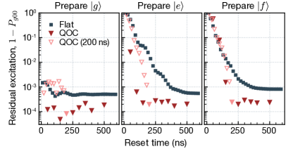
As a second demonstration of the adjoint state method, we consider the optimization of the f0-g1 reset of a transmon [48, 74, 49]. This is an all-microwave reset protocol based on a Raman transition between states $\ket{f00}$ and $\ket{g01}$. For the ket $\ket{ijk}$, $\ket{i}$ stands for the qubit state and $\ket{jk}$ the resonator-filter normal modes. Given the large photon loss rate of the filter, the state $\ket{g01}$ quickly decays to $\ket{g00}$, thus ensuring a fast reset of the transmon $\ket{f}$ state. An additional drive at the $\ket{e}$-$\ket{f}$ transition frequency allows to reset both $\ket{e}$ and $\ket{f}$ states of the transmon. We use the adjoint-state method to find optimal controls for both the f0-g1 and e-f drives simultaneously, in a similar fashion as for optimizing the readout. The cost function is now principally maximizing the transmon population in the $\ket{g00}$ state at the end of the protocol, along with smaller contributions for regularizing the pulses, see [52] for details.

The results of the reset optimization are summarized in Fig. 3. The three panels show the residual excitation out of $\ket{g00}$ against the reset time for a reference flat pulse (blue) and an optimized pulse (red) for different initial transmon states. The reference pulse is composed of two constant drives at the f0-g1 and e-f transitions, where amplitudes and frequencies are calibrated numerically in a similar fashion to what is done in experiments, see [52]. The QOC pulse is obtained by optimizing the carrier frequency and envelopes of both drives, for several total reset times. The optimized pulses show significant improvement over the reference, with a residual excitation of less than 0.05 % at $100\text{\,}\mathrm{ns}$ ($200\text{\,}\mathrm{ns}$) for the $\ket{e}$ ($\ket{f}$) state preparation. Note that this delay in the $\ket{f}$ reset time is due to a larger relative weight for the reset of $\ket{e}$ chosen in the cost function, and could be adjusted to achieve the most experimentally relevant reset scheme. This represents a notable improvement over the reference pulses, which reach a steady state after more than $300\text{\,}\mathrm{ns}$ with larger residual excitations of about 0.07 %. Our results also favourably compare to state-of-the-art experimental realizations of this protocol that reach 1.7 % residual excitations in $100\text{\,}\mathrm{ns}$ [47], or 0.3 % in $300\text{\,}\mathrm{ns}$ [49].

Conclusion.—

We obtained a fully general framework to optimize open quantum system dynamics in large Hilbert spaces by combining the adjoint state method and reverse-time back-propagation. We have demonstrated the applicability of this method to complex open-system optimization problems using the example of superconducting transmon readout and reset. We stress that our method can readily be applied to optimizing a wide range of quantum control problems where the dissipative dynamics play a significant role such as reservoir (dissipation) engineering [75, 76], autonomous QEC [77, 78], leakage-reduction units [79], quantum cooling, and more. We encourage readers to apply this framework on their own optimal control problems using the open-source library dynamiqs [57].

References

- Peirce et al. [1988] A. P. Peirce, M. A. Dahleh, and H. Rabitz, Optimal control of quantum-mechanical systems: Existence, numerical approximation, and applications, Phys. Rev. A 37, 4950 (1988).
- Werschnik and Gross [2007] J. Werschnik and E. Gross, Quantum optimal control theory, Journal of Physics B: Atomic, Molecular and Optical Physics 40, R175 (2007).
- Koch et al. [2022] C. P. Koch, U. Boscain, T. Calarco, G. Dirr, S. Filipp, S. J. Glaser, R. Kosloff, S. Montangero, T. Schulte-Herbrüggen, D. Sugny, and F. K. Wilhelm, Quantum optimal control in quantum technologies. strategic report on current status, visions and goals for research in europe, EPJ Quantum Technology 9, 10.1140/epjqt/s40507-022-00138-x (2022).
- Terhal [2015] B. M. Terhal, Quantum error correction for quantum memories, Rev. Mod. Phys. 87, 307 (2015).
- Günther et al. [2021] S. Günther, N. A. Petersson, and J. L. DuBois, Quantum optimal control for pure-state preparation using one initial state, AVS Quantum Science 3 (2021).
- Petruhanov and Pechen [2022] V. N. Petruhanov and A. N. Pechen, Optimal control for state preparation in two-qubit open quantum systems driven by coherent and incoherent controls via grape approach, International Journal of Modern Physics A 37, 2243017 (2022).
- Cai et al. [2021] W. Cai, Y. Ma, W. Wang, C.-L. Zou, and L. Sun, Bosonic quantum error correction codes in superconducting quantum circuits, Fundamental Research 1, 50–67 (2021).
- Motzoi et al. [2009] F. Motzoi, J. M. Gambetta, P. Rebentrost, and F. K. Wilhelm, Simple pulses for elimination of leakage in weakly nonlinear qubits, Phys. Rev. Lett. 103, 110501 (2009).
- Goerz et al. [2017] M. H. Goerz, F. Motzoi, K. B. Whaley, and C. P. Koch, Charting the circuit qed design landscape using optimal control theory, npj Quantum Information 3, 37 (2017).
- Werninghaus et al. [2021] M. Werninghaus, D. J. Egger, F. Roy, S. Machnes, F. K. Wilhelm, and S. Filipp, Leakage reduction in fast superconducting qubit gates via optimal control, npj Quantum Information 7, 10.1038/s41534-020-00346-2 (2021).
- Jandura and Pupillo [2022] S. Jandura and G. Pupillo, Time-optimal two- and three-qubit gates for rydberg atoms, Quantum 6, 712 (2022).
- Viola et al. [1999] L. Viola, E. Knill, and S. Lloyd, Dynamical decoupling of open quantum systems, Phys. Rev. Lett. 82, 2417 (1999).
- Khodjasteh and Lidar [2005] K. Khodjasteh and D. A. Lidar, Fault-tolerant quantum dynamical decoupling, Phys. Rev. Lett. 95, 180501 (2005).
- Biercuk et al. [2009] M. J. Biercuk, H. Uys, A. P. VanDevender, N. Shiga, W. M. Itano, and J. J. Bollinger, Optimized dynamical decoupling in a model quantum memory, Nature 458, 996 (2009).
- Koch [2016] C. P. Koch, Controlling open quantum systems: tools, achievements, and limitations, Journal of Physics: Condensed Matter 28, 213001 (2016).
- Kallush et al. [2022] S. Kallush, R. Dann, and R. Kosloff, Controlling the uncontrollable: Quantum control of open-system dynamics, Science Advances 8, eadd0828 (2022).
- Goerz et al. [2014] M. H. Goerz, D. M. Reich, and C. P. Koch, Optimal control theory for a unitary operation under dissipative evolution, New Journal of Physics 16, 055012 (2014).
- Propson et al. [2022] T. Propson, B. E. Jackson, J. Koch, Z. Manchester, and D. I. Schuster, Robust quantum optimal control with trajectory optimization, Phys. Rev. Appl. 17, 014036 (2022).
- An et al. [2021] Z. An, H.-J. Song, Q.-K. He, and D. L. Zhou, Quantum optimal control of multilevel dissipative quantum systems with reinforcement learning, Phys. Rev. A 103, 012404 (2021).
- Egger and Wilhelm [2014] D. J. Egger and F. K. Wilhelm, Optimal control of a quantum measurement, Phys. Rev. A 90, 052331 (2014).
- Boutin et al. [2017] S. Boutin, C. K. Andersen, J. Venkatraman, A. J. Ferris, and A. Blais, Resonator reset in circuit qed by optimal control for large open quantum systems, Phys. Rev. A 96, 042315 (2017).
- Krotov [1995] V. Krotov, Global methods in optimal control theory, Vol. 195 (CRC Press, 1995).
- Khaneja et al. [2005] N. Khaneja, T. Reiss, C. Kehlet, T. Schulte-Herbrüggen, and S. J. Glaser, Optimal control of coupled spin dynamics: design of nmr pulse sequences by gradient ascent algorithms, Journal of Magnetic Resonance 172, 296 (2005).
- Schulte-Herbrüggen et al. [2011] T. Schulte-Herbrüggen, A. Spörl, N. Khaneja, and S. Glaser, Optimal control for generating quantum gates in open dissipative systems, Journal of Physics B: Atomic, Molecular and Optical Physics 44, 154013 (2011).
- Goerz et al. [2019] M. Goerz, D. Basilewitsch, F. Gago-Encinas, M. G. Krauss, K. P. Horn, D. M. Reich, and C. Koch, Krotov: A python implementation of krotov’s method for quantum optimal control, SciPost physics 7, 080 (2019).
- Chen et al. [2020] H. Chen, H. Li, F. Motzoi, L. Martin, K. B. Whaley, and M. Sarovar, Quantum proportional-integral (pi) control, New Journal of Physics 22, 113014 (2020).
- Porotti et al. [2023] R. Porotti, V. Peano, and F. Marquardt, Gradient-ascent pulse engineering with feedback, PRX Quantum 4, 030305 (2023).
- Sivak et al. [2022] V. V. Sivak, A. Eickbusch, H. Liu, B. Royer, I. Tsioutsios, and M. H. Devoret, Model-free quantum control with reinforcement learning, Phys. Rev. X 12, 011059 (2022).
- Sivak et al. [2023] V. Sivak, A. Eickbusch, B. Royer, S. Singh, I. Tsioutsios, S. Ganjam, A. Miano, B. Brock, A. Ding, L. Frunzio, et al., Real-time quantum error correction beyond break-even, Nature 616, 50–55 (2023).
- Baum et al. [2021] Y. Baum, M. Amico, S. Howell, M. Hush, M. Liuzzi, P. Mundada, T. Merkh, A. R. Carvalho, and M. J. Biercuk, Experimental deep reinforcement learning for error-robust gate-set design on a superconducting quantum computer, PRX Quantum 2, 040324 (2021).
- Ding et al. [2023] L. Ding, M. Hays, Y. Sung, B. Kannan, J. An, A. Di Paolo, A. H. Karamlou, T. M. Hazard, K. Azar, D. K. Kim, B. M. Niedzielski, A. Melville, M. E. Schwartz, J. L. Yoder, T. P. Orlando, S. Gustavsson, J. A. Grover, K. Serniak, and W. D. Oliver, High-fidelity, frequency-flexible two-qubit fluxonium gates with a transmon coupler, Phys. Rev. X 13, 031035 (2023).
- Jirari [2009] H. Jirari, Optimal control approach to dynamical suppression of decoherence of a qubit, Europhysics Letters 87, 40003 (2009).
- Leung et al. [2017] N. Leung, M. Abdelhafez, J. Koch, and D. Schuster, Speedup for quantum optimal control from automatic differentiation based on graphics processing units, Phys. Rev. A 95, 042318 (2017).
- Baydin et al. [2018] A. G. Baydin, B. A. Pearlmutter, A. A. Radul, and J. M. Siskind, Automatic differentiation in machine learning: a survey, Journal of Marchine Learning Research 18, 1 (2018).
- Abdelhafez et al. [2019] M. Abdelhafez, D. I. Schuster, and J. Koch, Gradient-based optimal control of open quantum systems using quantum trajectories and automatic differentiation, Phys. Rev. A 99, 052327 (2019).
- Lu et al. [2023] Y. Lu, S. Joshi, V. S. Dinh, and J. Koch, Optimal control of large quantum systems: assessing memory and runtime performance of GRAPE, arXiv (2023), 2304.06200 .
- Pontryagin et al. [1962] L. Pontryagin, V. Boltyanskii, R. Gamkrelidze, and E. Mishechenko, The Mathematical Theory of Optimal Processes (CRC Press, 1962).
- Dehaghani and Aguiar [2023] N. B. Dehaghani and A. P. Aguiar, An application of pontryagin neural networks to solve optimal quantum control problems, arXiv preprint (2023), 2302.09143 .
- Boscain et al. [2021] U. Boscain, M. Sigalotti, and D. Sugny, Introduction to the pontryagin maximum principle for quantum optimal control, PRX Quantum 2, 030203 (2021).
- Chen et al. [2018] R. T. Chen, Y. Rubanova, J. Bettencourt, and D. K. Duvenaud, Neural ordinary differential equations, Advances in neural information processing systems 31 (2018).
- Kidger [2022] P. Kidger, On neural differential equations, Ph.D. thesis, Mathematical Institute, University of Oxford (2022), 2202.02435 .
- Somlói et al. [1993] J. Somlói, V. A. Kazakov, and D. J. Tannor, Controlled dissociation of i2 via optical transitions between the x and b electronic states, Chemical physics 172, 85 (1993).
- Goerz et al. [2022] M. H. Goerz, S. C. Carrasco, and V. S. Malinovsky, Quantum optimal control via semi-automatic differentiation, Quantum 6, 871 (2022).
- Narayanan et al. [2022] S. H. K. Narayanan, T. Propson, M. Bongarti, J. Hückelheim, and P. Hovland, Reducing memory requirements of quantum optimal control, in International Conference on Computational Science (Springer, 2022) pp. 129–142.
- Blais et al. [2004] A. Blais, R.-S. Huang, A. Wallraff, S. M. Girvin, and R. J. Schoelkopf, Cavity quantum electrodynamics for superconducting electrical circuits: An architecture for quantum computation, Phys. Rev. A 69, 062320 (2004).
- Walter et al. [2017] T. Walter, P. Kurpiers, S. Gasparinetti, P. Magnard, A. Potočnik, Y. Salathé, M. Pechal, M. Mondal, M. Oppliger, C. Eichler, and A. Wallraff, Rapid high-fidelity single-shot dispersive readout of superconducting qubits, Phys. Rev. Appl. 7, 054020 (2017).
- Sunada et al. [2022] Y. Sunada, S. Kono, J. Ilves, S. Tamate, T. Sugiyama, Y. Tabuchi, and Y. Nakamura, Fast readout and reset of a superconducting qubit coupled to a resonator with an intrinsic purcell filter, Phys. Rev. Appl. 17, 044016 (2022).
- Pechal et al. [2014] M. Pechal, L. Huthmacher, C. Eichler, S. Zeytinoğlu, A. A. Abdumalikov, S. Berger, A. Wallraff, and S. Filipp, Microwave-controlled generation of shaped single photons in circuit quantum electrodynamics, Phys. Rev. X 4, 041010 (2014).
- Magnard et al. [2018] P. Magnard, P. Kurpiers, B. Royer, T. Walter, J.-C. Besse, S. Gasparinetti, M. Pechal, J. Heinsoo, S. Storz, A. Blais, and A. Wallraff, Fast and unconditional all-microwave reset of a superconducting qubit, Phys. Rev. Lett. 121, 060502 (2018).
- Koch et al. [2007] J. Koch, T. M. Yu, J. Gambetta, A. A. Houck, D. I. Schuster, J. Majer, A. Blais, M. H. Devoret, S. M. Girvin, and R. J. Schoelkopf, Charge-insensitive qubit design derived from the cooper pair box, Phys. Rev. A 76, 042319 (2007).
- Gardiner and Zoller [2004] C. Gardiner and P. Zoller, Quantum noise: a handbook of Markovian and non-Markovian quantum stochastic methods with applications to quantum optics (Springer Science & Business Media, 2004).
- [52] See Supplemental Material for more information.
- Broyden [1970] C. G. Broyden, The convergence of a class of double-rank minimization algorithms 1. general considerations, IMA Journal of Applied Mathematics 6, 76 (1970).
- Kingma and Ba [2014] D. P. Kingma and J. Ba, Adam: A method for stochastic optimization, arXiv https://doi.org/10.48550/arXiv.1412.6980 (2014), 1412.6980 .
- Robbins and Monro [1951] H. Robbins and S. Monro, A Stochastic Approximation Method, The Annals of Mathematical Statistics 22, 400 (1951).
- Paszke et al. [2019] A. Paszke, S. Gross, F. Massa, A. Lerer, J. Bradbury, G. Chanan, T. Killeen, Z. Lin, N. Gimelshein, L. Antiga, et al., Pytorch: An imperative style, high-performance deep learning library, Advances in neural information processing systems 32 (2019), 1912.01703 .
- Guilmin et al. [2024] P. Guilmin, R. Gautier, A. Bocquet, and E. Genois, dynamiqs: an open-source library for GPU-accelerated and differentiable simulation of quantum systems (2024), in preparation, library available at dynamiqs.org.
- Blais et al. [2021] A. Blais, A. L. Grimsmo, S. M. Girvin, and A. Wallraff, Circuit quantum electrodynamics, Rev. Mod. Phys. 93, 025005 (2021).
- Cohen et al. [2023] J. Cohen, A. Petrescu, R. Shillito, and A. Blais, Reminiscence of classical chaos in driven transmons, PRX Quantum 4, 020312 (2023).
- Shillito et al. [2022] R. Shillito, A. Petrescu, J. Cohen, J. Beall, M. Hauru, M. Ganahl, A. G. Lewis, G. Vidal, and A. Blais, Dynamics of transmon ionization, Phys. Rev. Appl. 18, 034031 (2022).
- Dumas et al. [2024] M. F. Dumas, B. Groleau-Paré, A. McDonald, M. H. Muñoz-Arias, C. Lledó, B. D’Anjou, and A. Blais, Unified picture of measurement-induced ionization in the transmon (2024), arXiv:2402.06615 .
- Swiadek et al. [2023] F. Swiadek, R. Shillito, P. Magnard, A. Remm, C. Hellings, N. Lacroix, Q. Ficheux, D. C. Zanuz, G. J. Norris, A. Blais, et al., Enhancing dispersive readout of superconducting qubits through dynamic control of the dispersive shift: Experiment and theory, arXiv (2023), 2307.07765 .
- Bultink et al. [2018] C. C. Bultink, B. Tarasinski, N. Haandbæk, S. Poletto, N. Haider, D. Michalak, A. Bruno, and L. DiCarlo, General method for extracting the quantum efficiency of dispersive qubit readout in circuit qed, Applied Physics Letters 112, https://doi.org/10.1063/1.5015954 (2018).
- Gambetta et al. [2007] J. Gambetta, W. A. Braff, A. Wallraff, S. M. Girvin, and R. J. Schoelkopf, Protocols for optimal readout of qubits using a continuous quantum nondemolition measurement, Phys. Rev. A 76, 012325 (2007).
- Motzoi et al. [2011] F. Motzoi, J. M. Gambetta, S. T. Merkel, and F. K. Wilhelm, Optimal control methods for rapidly time-varying hamiltonians, Phys. Rev. A 84, 022307 (2011).
- Sunada et al. [2024] Y. Sunada, K. Yuki, Z. Wang, T. Miyamura, J. Ilves, K. Matsuura, P. A. Spring, S. Tamate, S. Kono, and Y. Nakamura, Photon-noise-tolerant dispersive readout of a superconducting qubit using a nonlinear purcell filter, PRX Quantum 5, 010307 (2024).
- Ikonen et al. [2019] J. Ikonen, J. Goetz, J. Ilves, A. Keränen, A. M. Gunyho, M. Partanen, K. Y. Tan, D. Hazra, L. Grönberg, V. Vesterinen, S. Simbierowicz, J. Hassel, and M. Möttönen, Qubit measurement by multichannel driving, Phys. Rev. Lett. 122, 080503 (2019).
- Touzard et al. [2019] S. Touzard, A. Kou, N. E. Frattini, V. V. Sivak, S. Puri, A. Grimm, L. Frunzio, S. Shankar, and M. H. Devoret, Gated conditional displacement readout of superconducting qubits, Phys. Rev. Lett. 122, 080502 (2019).
- Muñoz Arias et al. [2023] M. H. Muñoz Arias, C. Lledó, and A. Blais, Qubit readout enabled by qubit cloaking, Phys. Rev. Appl. 20, 054013 (2023).
- Mallet et al. [2009] F. Mallet, F. R. Ong, A. Palacios-Laloy, F. Nguyen, P. Bertet, D. Vion, and D. Esteve, Single-shot qubit readout in circuit quantum electrodynamics, Nat Phys 5, 791 (2009).
- D’Anjou and Coish [2017] B. D’Anjou and W. A. Coish, Enhancing qubit readout through dissipative sub-poissonian dynamics, Phys. Rev. A 96, 052321 (2017).
- Elder et al. [2020] S. S. Elder, C. S. Wang, P. Reinhold, C. T. Hann, K. S. Chou, B. J. Lester, S. Rosenblum, L. Frunzio, L. Jiang, and R. J. Schoelkopf, High-fidelity measurement of qubits encoded in multilevel superconducting circuits, Phys. Rev. X 10, 011001 (2020).
- Chen et al. [2023] L. Chen, H.-X. Li, Y. Lu, C. W. Warren, C. J. Križan, S. Kosen, M. Rommel, S. Ahmed, A. Osman, J. Biznárová, et al., Transmon qubit readout fidelity at the threshold for quantum error correction without a quantum-limited amplifier, npj Quantum Information 9, 26 (2023).
- Zeytinoğlu et al. [2015] S. Zeytinoğlu, M. Pechal, S. Berger, A. A. Abdumalikov, A. Wallraff, and S. Filipp, Microwave-induced amplitude- and phase-tunable qubit-resonator coupling in circuit quantum electrodynamics, Phys. Rev. A 91, 043846 (2015).
- Poyatos et al. [1996] J. F. Poyatos, J. I. Cirac, and P. Zoller, Quantum reservoir engineering with laser cooled trapped ions, Phys. Rev. Lett. 77, 4728 (1996).
- Harrington et al. [2022] P. M. Harrington, E. Mueller, and K. Murch, Engineered dissipation for quantum information science (2022), arXiv:2202.05280 [quant-ph] .
- Royer et al. [2020] B. Royer, S. Singh, and S. M. Girvin, Stabilization of finite-energy gottesman-kitaev-preskill states, Phys. Rev. Lett. 125, 260509 (2020).
- Gertler et al. [2021] J. M. Gertler, B. Baker, J. Li, S. Shirol, J. Koch, and C. Wang, Protecting a bosonic qubit with autonomous quantum error correction, Nature 590, 243–248 (2021).
- Aliferis and Terhal [2007] P. Aliferis and B. M. Terhal, Fault-tolerant quantum computation for local leakage faults, Quantum Info. Comput. 7, 139–156 (2007).