Noisy atomic magnetometry with Kalman filtering and measurement-based feedback

Abstract

Tracking a magnetic field in real-time with an atomic magnetometer presents significant challenges, primarily due to sensor non-linearity, the presence of noise, and the need for one-shot estimation. To address these challenges, we propose a comprehensive approach that integrates measurement, estimation and control strategies. Specifically, this involves implementing a quantum non-demolition measurement based on continuous light-probing of the atomic ensemble. The resulting photocurrent is then directed into an Extended Kalman Filter to produce instantaneous estimates of the system’s dynamical parameters. These estimates, in turn, are utilised by a Linear Quadratic Regulator, whose output is applied back to the system through a feedback loop. This procedure automatically steers the atomic ensemble into a spin-squeezed state, yielding a quantum enhancement in precision. Furthermore, thanks to the feedback proposed, the atoms exhibit entanglement even when the measurement data is discarded. To prove that our approach constitutes the optimal strategy in realistic scenarios, we derive ultimate bounds on the estimation error applicable in the presence of both local and collective decoherence, and show that these are indeed attained. Additionally, we demonstrate for large ensembles that the EKF not only reliably predicts its own estimation error in real time, but also accurately estimates spin-squeezing at short timescales.

I Introduction

Optical magnetometers that rely on atomic ensembles pumped and probed with laser light [1] constitute ultraprecise magnetic field sensors, achieving sensitivities comparable to the state-of-the-art SQUID-based devices [2]. Not only do they not require cryogenic cooling, but also they have been recently miniaturised to chip scales [3]. As a result, they promise breakthroughs, e.g., when used to sense magnetic fields in medical applications [4, 5, 6, 7], as well as in the search for new exotic physics [8, 9]. These tasks, in particular, fall into the category of real-time sensing problems in which the sensor is employed to track a time-varying signal (magnetic field) while continuously acquiring measurement data. Such a scenario may be considered the most demanding, as it requires the sensing procedure to be performed only once, with the sensor being controlled “on the fly”. Despite some prominent achievements [10, 11, 12], there is yet to be an experimental demonstration showing that sensing performance can be significantly improved by employing quantum effects, i.e.: the inter-atomic entanglement induced by measurement back-action [13], which has already been shown to strongly enhance precision in the setting of multiple independent and identical (iid) repetitions [14, 15, 16]. Apart from sophisticated experimental challenges, an important hurdle is also the proposal and verification of an accurate dynamic model of the atomic noise, which would then allow for the tools of control and statistical inference theory to be used in the design of a future device. This contrasts with the setting of, e.g., optomechanical sensors [17]—operating typically at cryogenic temperatures—in which case quantum stochastic models have been proposed and verified [18, 19], allowing for spectacular demonstrations of cooling and controlling of such devices in real time [20], while incorporating both measurement-based [21, 22, 23] (also with use of levitated nanoparticles [24, 25]) and coherent [26] feedback methods [27, 28, 29].

In our work, building on the theory of continuously monitored atomic ensembles that are optically pumped with circularly polarised light [30, 31, 32], we propose and simulate for the first time—employing novel numerical tools [33]—a quantum dynamical model that allows us, on one hand, to study in detail the precision in sensing a constant magnetic field while benefiting from the atomic spin-squeezing [34]. On the other hand, it incorporates both mechanisms of local and collective atomic decoherence, allowing us to verify the robustness of the protocol. Stemming from our previous results [35], we show how such forms of noise impose ultimate limits on the achievable precision for any protocol involving measurement-based feedback and, hence, disallow the possibility of surpassing the standard quantum limit (SQL) despite decoherence, as previously conjectured based on numerical evidence [36]. However, we demonstrate that these noise-induced ultimate bounds that still require interatomic entanglement can be, in fact, saturated by resorting to the estimation and control procedure consisting of an Extended Kalman Filter (EKF) [37, 38] and a Linear Quadratic Regulator (LQR) [31, 25]. In particular, we demonstrate the optimality of our proposal for sensors involving a large number of atoms ($N\approx 10^{5}\!-\!10^{13}$ in typical experiments [10, 16, 11, 15, 14, 12]) and operated at short times. In this regime, we accurately capture the overall spin dynamics by using the co-moving Gaussian approximation [39], which we initially introduce to construct the EKF. Moreover, this approximate simulation of the spin dynamics enables us to reliably model the conditional spin-squeezing [40], which would otherwise be inaccessible with exact numerical simulations for large ensembles. Importantly, this allows us to verify that the EKF accurately estimates then the conditional spin-squeezing based only on the measurement record.

Our work paves the way for the use of non-linear atomic systems as magnetic sensors, through the combination of EKF with LQR. Moreover, as we show this measurement-based feedback strategy to also generate unconditional spin-squeezing—namely, to automatically steer the atomic ensemble into a state whose interatomic entanglement can be verified without the need to store particular measurement trajectories— we believe that the EKF+LQR strategy provides a new, useful tool for real-time quantum state engineering per se.

The manuscript is organised as follows: in Sec. II we present the setup of the atomic magnetometer we choose to consider. Sec. III discusses the numerical simulation of the exact sensor model and how to approximate it by introducing the co-moving Gaussian picture. Then, in Sec. IV, we build upon the work of Ref. [35] by extending it to include local decoherence, and establish ultimate bounds on the achievable precision in magnetic-field estimation. Subsequently, in Sec. V, we detail our chosen estimation and control strategies, namely EKF and LQR. The final two sections, Sec. VI and Sec. VII, present our results. Specifically, section VI demonstrates that in the large $N$ regime, our proposed EKF+LQR strategy can attain the noise-induced ultimate bounds on precision. Moreover, Sec. VII reveals that the introduction of LQR feedback prepares the atomic state in a multipartite entangled state, as indicated by the emergence of unconditional spin-squeezing. Finally, Sec. VIII summarises our results and discusses their implications.

II Setup

The main goal of the magnetometry experiment depicted in Fig. 1 is to estimate the magnetic field $B$ aligned with the $z$-axis. For the sake of simplicity, we consider here the situation in which $B$ is unknown but of constant value, setting aside the estimation of time-varying and fluctuating magnetic fields for separate work [41]. An ensemble of $N$ atoms is used to indirectly probe the magnetic field $B$, while being pumped with circularly polarised light along the $x$-direction, see Fig. 1, such that only two energy levels of each atom effectively contribute to the light-probing process [42]. As a consequence, we may treat the atomic ensemble as a collection of $N$ spin-$1/2$ particles, whose spin precesses around the $z$-axis at a Larmor frequency $\omega=\gamma B$ induced by the magnetic field $B$, where $\gamma$ is the gyromagnetic ratio. Moreover, the evolution of the total spin is then described through the use of collective angular momentum operators, $\hat{J}_{\alpha}=\sum_{i=1}^{N}\hat{\sigma}_{\alpha}^{(i)}/2$ with $\alpha=x,y,z$, that form an (orientation) vector $\hat{\boldsymbol{J}\hskip 2.84544pt}=(\hat{J}_{x},\hat{J}_{y},\hat{J}_{z})^{\mathsf{T}}$.

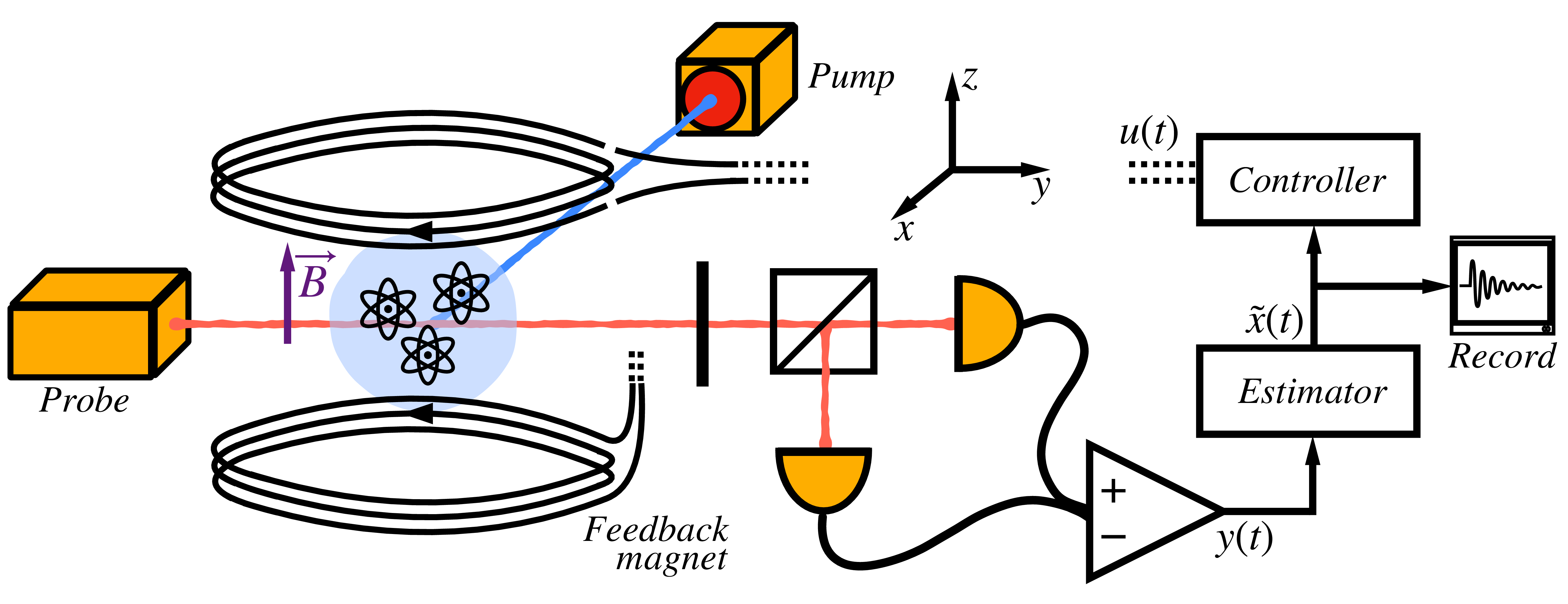
Figure 1: Atomic magnetometry with estimation and control. The magnetometer consists of an ensemble of spin-1/2 atoms, initially pumped along $x$ into a coherent spin state, which then Larmor-precess around the $z$-axis due to the constant magnetic field $B$ to be determined. The total atomic spin is probed along the $y$-direction by the second beam that weakly interacts with the ensemble, so that the corresponding spin-component can be continuously monitored via balanced photodetection. The output photocurrent $y(t)$ is then used to construct estimates of the temporary dynamical parameters of the atomic ensemble, $\boldsymbol{\tilde{x}}(t)$ (containing also the $B$-field estimate), and feed them into the controller that instantaneously decides on the value, $u(t)$, of the extra magnetic field to be induced through the feedback coil, so that arbitrary bias can be applied in real time to the estimated magnetic field $B$.

Furthermore, assuming the atoms are initially pumped (along $x$, see Fig. 1) into a coherent spin state (CSS), the mean and the variance for each component of $\hat{\boldsymbol{J}\hskip 2.84544pt}(t)$ are given at time $t=0$ by $\langle\hat{\boldsymbol{J}\hskip 2.84544pt}\rangle_{\textsc{css}}=(N/2,0,0)^{\mathsf{T}}$ and $\boldsymbol{\mathrm{V}}^{\textsc{css}}=(0,N/4,N/4)^{\mathsf{T}}$ [34], respectively, where $\mathrm{V}_{\alpha}^{\textsc{css}}\coloneqq\langle\hat{J}_{\alpha}^{2}\rangle_{\textsc{css}}-\langle\hat{J}_{\alpha}\rangle_{\textsc{css}}^{2}$. However, as explicitly shown in Fig. 2, it is useful to visualise such a state as a quasiprobability distribution on a (generalised) Bloch sphere—formally the Wigner function projected onto a sphere, see App. A [40]—which is centred at $\langle\hat{\boldsymbol{J}\hskip 2.84544pt}\rangle_{\textsc{css}}$ with the width in the $xyz$-directions specified by the elements of $\boldsymbol{\mathrm{V}}^{\textsc{css}}$.

Once pumped, the atoms are continuously monitored by a linearly polarised probe beam directed along the $y$-axis, as shown in Fig. 1. The probe light is sufficiently detuned from the relevant atomic transition, so that its interaction with the atoms can be considered linear while still inducing back-action due to the quantum non-demolition character of the measurement [43, 32]. In particular, upon interaction with the atoms the probe-beam polarisation gets (Faraday) rotated by an angle proportional to the total angular momentum component along the probe propagation, i.e. $\hat{J}_{y}$. As a result, the output photocurrent of a differential photo-detection measurement, which registers small polarisation-angle deviations, is given by [44, 45]:

$$y(t)dt=2\eta\sqrt{M}\big{\langle}\hat{J}_{y}(t)\big{\rangle}_{\!\scriptscriptstyle\mathrm{(c)}}dt+\sqrt{\eta}\,dW,$$ (1)

where $\eta$ is the detection efficiency and $dW$ denotes the stochastic Wiener increment, satisfying $\mathbb{E}\!\left[dW^{2}\right]=dt$ according to Itô calculus [46]. The white-noise fluctuations in Eq. (1) arise due to the shot noise of the photo-detection process. However, by fixing their strength to unity, we effectively renormalise the photocurrent $y(t)$. As a result, it is the measurement strength parameter $M$ that—while incorporating all the relevant experimental electronic, light-matter couplings etc. [43]—parametrises the ratio between the atomic contribution to the detected signal (first term in Eq. (1)) and the magnitude of white-noise (second term in Eq. (1)).

An essential feature of the above formalism is the incorporation of measurement back-action exerted onto the atoms [44, 45]. In particular, within Eq. (1), the mean $\big{\langle}\hat{J}_{y}(t)\big{\rangle}_{\!\scriptscriptstyle\mathrm{(c)}}=\mathrm{Tr}\!\left\{\rho_{\scriptscriptstyle\mathrm{(c)}}(t)\hat{J}_{y}\right\}$ is evaluated with respect to the conditional atomic state, $\rho_{\scriptscriptstyle\mathrm{(c)}}(t)\equiv\rho(t|\boldsymbol{y}_{\leq t})$, i.e. the one most consistent (minimising the mean-square distance [45]) with the particular measurement trajectory observed, $\boldsymbol{y}_{\leq t}=\{y(\tau)\}_{0\leq\tau\leq t}$. Additionally, to explicitly write the dynamics of $\rho_{\scriptscriptstyle\mathrm{(c)}}(t)$, we must also account for the measurement-based control strategy introduced in Fig. 1. This strategy assumes that based on the photocurrent record (potentially whole history), $\boldsymbol{y}_{\leq t}$, estimates of some dynamical parameters for the atomic system are made—denoted by a vector $\tilde{\boldsymbol{x}}(t)$ in Fig. 1, which includes the estimate of the Larmor frequency, $\tilde{\omega}=\gamma\tilde{B}$, and hence the $B$-field. The estimates, $\tilde{\boldsymbol{x}}(t)$, are then used to set the control (scalar) field to a specific value $u(\boldsymbol{y}_{\leq t})$, altering the additional magnetic field applied instantaneously along the estimated $B$ and thus modifying the Larmor frequency at time $t$ to: $\omega\to\omega+u(\boldsymbol{y}_{\leq t})$. As the control field $u(\boldsymbol{y}_{\leq t})$ depends on the whole measurement record $\boldsymbol{y}_{\leq t}$, the dynamics of the atomic ensemble at each time step are not only affected by the back-action of the current measurement but also dependent on the entire measurement record through the addition of control.

Bearing this in mind and simplifying notation by denoting the control field as $u(t)\equiv u(\boldsymbol{y}_{\leq t})$, we write the stochastic master equation (SME) that governs the dynamics of the conditional atomic state $\rho_{\scriptscriptstyle\mathrm{(c)}}(t)$ as [44, 45]:

$$d\rho_{\scriptscriptstyle\mathrm{(c)}}= -i(\omega+u(t))[\hat{J}_{z},\rho_{\scriptscriptstyle\mathrm{(c)}}]dt$$

$$+\frac{\kappa_{\mathrm{loc}}}{2}\sum_{j=1}^{N}\mathcal{D}[\hat{\sigma}_{z}^{(j)}]\rho_{\scriptscriptstyle\mathrm{(c)}}dt\,+\kappa_{\mathrm{coll}}\mathcal{D}[\hat{J}_{z}]\rho_{\scriptscriptstyle\mathrm{(c)}}dt$$

$$+M\mathcal{D}[\hat{J}_{y}]\rho_{\scriptscriptstyle\mathrm{(c)}}dt+\sqrt{\eta M}\mathcal{H}[\hat{J}_{y}]\rho_{\scriptscriptstyle\mathrm{(c)}}dW,$$ (2)

where the superoperators $\mathcal{D}$ and $\mathcal{H}$ are defined for any operator $\hat{A}$ and state $\rho$ as $\mathcal{D}[\hat{A}]\rho\coloneqq\hat{A}\rho\hat{A}^{\dagger}-\frac{1}{2}\{\hat{A}^{\dagger}\hat{A},\rho\}$ and $\mathcal{H}[\hat{A}]\rho\coloneqq\hat{A}\rho+\rho\hat{A}^{\dagger}-\mathrm{Tr}\!\left\{(\hat{A}+\hat{A}^{\dagger})\rho\right\}\rho$.

The last two terms in Eq. (2) arise due the back-action of the continuous quantum measurement: the first term represents the measurement-induced decoherence in the basis of the observable being probed, $\hat{J}_{y}$; the second term accounts for the stochastic jump dictated by the photocurrent recorded during a particular time-step, $dW=[y(t)/\sqrt{\eta}-2\sqrt{\eta M}\big{\langle}\hat{J}_{y}\big{\rangle}_{\!\scriptscriptstyle\mathrm{(c)}}]dt$ according to Eq. (1). This last term, crucially nonlinear in $\rho_{\scriptscriptstyle\mathrm{(c)}}$, opens doors for conditional squeezing of the atomic state [30]. However, to account for the impact of noise and verify the robustness of our estimation strategies, we also incorporate in Eq. (2) local and global decoherence terms. These terms effectively dephase the atomic state along the $z$-direction of the estimated $B$-field at the rates $\kappa_{\mathrm{loc}}$ and $\kappa_{\mathrm{coll}}$ for local and collective dephasing, respectively. Local dephasing acts independently on each individual atom $j$ in the basis of $\hat{\sigma}_{z}^{(j)}/2$, while the collective term acts globally within the basis of the collective atomic spin operator $\hat{J}_{z}$.

III Simulating the system dynamics

III.1 Exact model: numerical solution

Optically pumped magnetometers operate with atomic numbers in the range of $N\approx 10^{5}\!-\!10^{13}$ [10, 16, 11, 15, 14, 12]. This precludes any naive numerical simulations of the ensemble dynamics, since the dimension of the underlying Hilbert space scaling exponentially with $N$, i.e. as $2^{N}$ for spin-$1/2$ atoms. However, assuming the system to preserve permutational invariance over the entire duration of its evolution, — meaning any pair of atoms within the ensemble is interchangeable — the dimension of the density matrix can be reduced to scale polynomially with $N$. In particular, for a collection of spin-$1/2$ atoms, as the density matrix possesses then a direct-sum structure with each block being associated with a spin-number $j$ ranging from $0$ $(\tfrac{1}{2})$ to $N/2$ for even (odd) $N$, its complexity scales as $O(N^{3})$ [47, 48, 49]. Moreover, if the evolution is induced by collective processes — i.e. generated by collective operators that are themselves permutationally invariant — any initial state supported by the totally symmetric subspace (with $j=N/2$), e.g. CSS, must evolve within it, further reducing the complexity to $O(N)$ [47, 48, 49].

In this work, we use the numerical solution of the SME (2) as a benchmark, which preserves the permutational symmetry (or even the totally symmetric subspace in case of $\kappa_{\mathrm{loc}}=0$). Specifically, for moderate $N$, we employ the code of Rossi et al. [33] that exploits the symmetries of the system as described above. It resorts to numerical integration of an SME by constructing the Kraus operators of the weak measurement at each time-step, while also guaranteeing the positivity of the density matrix [50, 51].

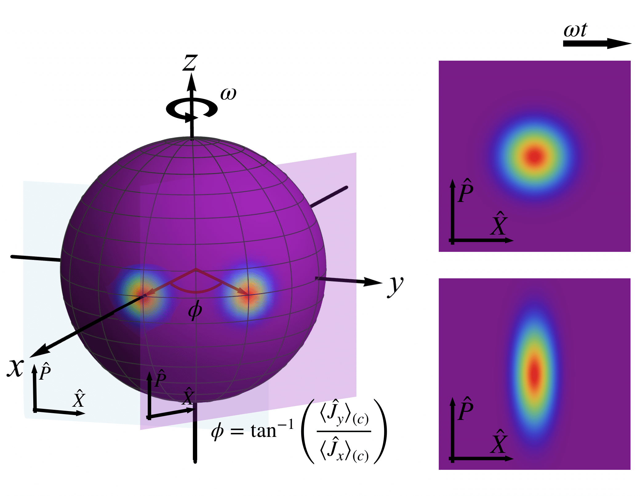
Figure 2: Bloch sphere representation of the atomic state: Linear-Gaussian (LG) and co-moving Gaussian (CoG) approximations. The 3D-plot depicts the Wigner function of a CSS pointing along $x$ in a generalised Bloch sphere for $N=100$. For large enough atomic ensembles, $N\gg 1$, the curvature of the sphere at the point where the Wigner function of the CSS is maximal can be approximated by the LG-plane, in which the effective phase-space quadratures, $\hat{X}$ and $\hat{P}$, can be defined as in Eq. (3). The continuous measurement of the $y$ spin-component, which induces spin-squeezing of the atomic state, can then be interpreted as just (anti)squeezing the ($\hat{P}$)$\hat{X}$ quadrature at short times at which the LG approximation still holds. In order for the Gaussian picture to remain valid at longer times, we let the LG-plane rotate at the Larmor frequency $\omega$ together with the atomic spin, and refer to such a description as the co-moving Gaussian (CoG) approximation.

III.2 Approximate model: co-moving Gaussian picture

III.2.1 Linear-Gaussian regime

Still, the exploitation of permutational symmetry is not sufficient to reach experimentally relevant values of $N$. One approach is to further assume that the $B$-field is small and the impact of local decoherence is negligible. As a result, by considering small enough timescales, $t\lesssim 1/(M+\kappa_{\mathrm{coll}})$, we can approximate $\big{\langle}\hat{J}_{x}(t)\big{\rangle}_{\!\scriptscriptstyle\mathrm{(c)}}$ with its unconditional average value $\langle\hat{J}_{x}(t)\rangle=\tfrac{N}{2}\mathrm{e}^{-(M+\kappa_{\mathrm{coll}})t/2}$ [35]. Geometrically, as depicted in Fig. 2, this corresponds to effectively approximating the surface of the generalised Bloch sphere by a plane perpendicular to the collective angular momentum vector pointing in the $x$-direction [30, 52, 35]. This plane then defines an effective phase space with position and momentum operators given by:

$$\hat{X}\coloneqq\hat{J}_{y}/\sqrt{|\langle\hat{J}_{x}(t)\rangle|},\;\;\text{and}\;\;\hat{P}\coloneqq\hat{J}_{z}/\sqrt{|\langle\hat{J}_{x}(t)\rangle|},$$ (3)

which satisfy the canonical commutation relation $[\hat{X},\hat{P}]\approx i$, as long as $\hat{J}_{x}\approx\left|\langle\hat{J}_{x}(t)\rangle\right|\openone$ for sufficiently large $N$ [53, 54]. As the SME (2) then becomes equivalent to a set of differential equations for first and second moments of the quadratures (3) that are linear in $\langle\hat{X}\rangle$ and $\langle\hat{P}\rangle$, as well as in the magnetic field $B$ [53, 54], we refer to such a regime as being linear-Gaussian (LG) [35].

III.2.2 Beyond the Linear-Gaussian regime

In real-life magnetometers [10, 16, 11, 15, 14, 12], the atomic spin must precess multiple times over the course of the detection process to collect a sufficient signal. This precludes the LG approximation from being actually useful. Therefore, to describe the system as approximately Gaussian at all times, we allow the LG-plane (see Fig. 2) to Larmor-precess with the mean angular-momentum vector $\langle\hat{\boldsymbol{J}\hskip 2.84544pt}(t)\rangle$ at the frequency $\omega$ [39]. We refer to this as the co-moving Gaussian (CoG) approximation. We expect this approach to be valid under the following conditions: the ensemble is large enough, i.e., $N\gg 1$; the squeezing due to the continuous measurement is not too strong to wrap the Wigner function around the Bloch sphere; and the local decoherence is moderate, allowing the dynamics to be well-described by only the first and second moments.

In particular, by considering the conditional evolution within the Heisenberg picture of the mean angular momenta $\big{\langle}\hat{J}_{\alpha}(t)\big{\rangle}_{\!\scriptscriptstyle\mathrm{(c)}}$, as well as their corresponding covariance matrix $\mathrm{C}^{\scriptscriptstyle\mathrm{(c)}}_{\alpha\beta}(t)\coloneqq\frac{1}{2}\left(\big{\langle}\{\hat{J}_{\alpha}(t),\hat{J}_{\beta}(t)\}\big{\rangle}_{\!\scriptscriptstyle\mathrm{(c)}}-2\big{\langle}\hat{J}_{\alpha}(t)\big{\rangle}_{\!\scriptscriptstyle\mathrm{(c)}}\big{\langle}\hat{J}_{\beta}(t)\big{\rangle}_{\!\scriptscriptstyle\mathrm{(c)}}\right)$ with diagonal elements $\mathrm{V}^{\scriptscriptstyle\mathrm{(c)}}_{\alpha}(t)\coloneqq\mathrm{C}^{\scriptscriptstyle\mathrm{(c)}}_{\alpha\alpha}(t)$ ($\alpha,\beta=x,y,z$), we derive in App. B based on the SME (2) the following set of coupled stochastic differential equations (dropping the explicit $t$-dependence of all the quantities for convenience):

$$d\big{\langle}\hat{J}_{x}\big{\rangle}_{\!\scriptscriptstyle\mathrm{(c)}}\!=\!-(\omega\!+\!u(t))\big{\langle}\hat{J}_{y}\big{\rangle}_{\!\scriptscriptstyle\mathrm{(c)}}dt\!-\frac{1}{2}(\kappa_{\mathrm{coll}}\!+\!2\kappa_{\mathrm{loc}}\!+\!M)\big{\langle}\hat{J}_{x}\big{\rangle}_{\!\scriptscriptstyle\mathrm{(c)}}dt\!+\!2\sqrt{\eta M}\mathrm{C}_{xy}^{\scriptscriptstyle\mathrm{(c)}}\,dW$$ (4a)

$$d\big{\langle}\hat{J}_{y}\big{\rangle}_{\!\scriptscriptstyle\mathrm{(c)}}\!=\!(\omega\!+\!u(t))\big{\langle}\hat{J}_{x}\big{\rangle}_{\!\scriptscriptstyle\mathrm{(c)}}dt\!-\frac{1}{2}(\kappa_{\mathrm{coll}}\!+\!2\kappa_{\mathrm{loc}})\big{\langle}\hat{J}_{y}\big{\rangle}_{\!\scriptscriptstyle\mathrm{(c)}}dt\!+\!2\sqrt{\eta M}\mathrm{V}_{y}^{\scriptscriptstyle\mathrm{(c)}}\,dW$$ (4b)

$$d\mathrm{V}_{x}^{\scriptscriptstyle\mathrm{(c)}}\!=\!-2(\omega\!+\!u(t))\mathrm{C}_{xy}^{\scriptscriptstyle\mathrm{(c)}}dt\!+\!\kappa_{\mathrm{coll}}\!\left(\!\mathrm{V}_{y}^{\scriptscriptstyle\mathrm{(c)}}\!+\!\big{\langle}\hat{J}_{y}\big{\rangle}_{\!\scriptscriptstyle\mathrm{(c)}}^{2}\!-\!\mathrm{V}_{x}^{\scriptscriptstyle\mathrm{(c)}}\!\right)\!dt\!+\!\kappa_{\mathrm{loc}}\!\left(\!\frac{N}{2}\!-\!2\mathrm{V}_{x}^{\scriptscriptstyle\mathrm{(c)}}\!\right)\!dt\!+\!M\!\left(\!\mathrm{V}_{z}^{\scriptscriptstyle\mathrm{(c)}}\!-\!\mathrm{V}_{x}^{\scriptscriptstyle\mathrm{(c)}}\!-\!4\eta{\mathrm{C}_{xy}^{\scriptscriptstyle\mathrm{(c)}}}^{2}\!\right)\!dt$$ (4c)

$$d\mathrm{V}_{y}^{\scriptscriptstyle\mathrm{(c)}}\!=\!2(\omega\!+\!u(t))\mathrm{C}_{xy}^{\scriptscriptstyle\mathrm{(c)}}dt\!+\!\kappa_{\mathrm{coll}}\!\left(\!\mathrm{V}_{x}^{\scriptscriptstyle\mathrm{(c)}}\!+\!\big{\langle}\hat{J}_{x}\big{\rangle}_{\!\scriptscriptstyle\mathrm{(c)}}^{2}\!-\!\mathrm{V}_{y}^{\scriptscriptstyle\mathrm{(c)}}\!\right)\!dt\!+\!\kappa_{\mathrm{loc}}\!\left(\!\frac{N}{2}\!-\!2\mathrm{V}_{y}^{\scriptscriptstyle\mathrm{(c)}}\!\right)\!dt\!-\!4\eta M{\mathrm{V}_{y}^{\scriptscriptstyle\mathrm{(c)}}}^{2}dt$$ (4d)

$$d\mathrm{V}_{z}^{\scriptscriptstyle\mathrm{(c)}}\!=\!M\!\left(\!\mathrm{V}_{x}^{\scriptscriptstyle\mathrm{(c)}}\!+\!\big{\langle}\hat{J}_{x}\big{\rangle}_{\!\scriptscriptstyle\mathrm{(c)}}^{2}\!-\!\mathrm{V}_{z}^{\scriptscriptstyle\mathrm{(c)}}\!\right)\!dt$$ (4e)

$$d\mathrm{C}_{xy}^{\scriptscriptstyle\mathrm{(c)}}\!=\!(\omega\!+\!u(t))\!\left(\!\mathrm{V}_{x}^{\scriptscriptstyle\mathrm{(c)}}\!-\!\mathrm{V}_{y}^{\scriptscriptstyle\mathrm{(c)}}\!\right)\!dt\!-\!\kappa_{\mathrm{coll}}\!\left(\!2\mathrm{C}_{xy}^{\scriptscriptstyle\mathrm{(c)}}\!+\!\big{\langle}\hat{J}_{x}\big{\rangle}_{\!\scriptscriptstyle\mathrm{(c)}}\big{\langle}\hat{J}_{y}\big{\rangle}_{\!\scriptscriptstyle\mathrm{(c)}}\!\right)\!dt\!-\!2\kappa_{\mathrm{loc}}\mathrm{C}_{xy}^{\scriptscriptstyle\mathrm{(c)}}dt\!-\!\frac{1}{2}M\mathrm{C}_{xy}^{\scriptscriptstyle\mathrm{(c)}}\left(1+8\eta\mathrm{V}_{y}^{\scriptscriptstyle\mathrm{(c)}}\right)\!dt$$ (4f)

$$d\omega\!=\!0,$$ (4g)

where in Eqs. (4c-4f) we importantly ignore all the (stochastic) contributions that involve the third-order moments, which can be found in App. B.

In what follows, we simulate the exact dynamics (2) of the density matrix for low values of $N$ to verify that the equations (4) correctly describe the evolution of the lowest moments for modest values of decoherence and measurement-strength parameters. As we observe the agreement to improve with the atomic number at short timescales (more details in App. F) for the experimentally relevant regimes of large $N\approx 10^{5}\!-\!10^{13}$ [10, 16, 11, 15, 14, 12], we subsequently use the equations (4) to simulate the dynamics of the atomic sensor with sufficient accuracy.

Crucially, regardless of the size of the ensemble, we construct the Extended Kalman filter (EKF) based on the nonlinear dynamical model (4). The output of the filter provides us with real-time estimates of dynamical parameters, i.e. of $\boldsymbol{x}(t)=(\big{\langle}\hat{J}_{x}\big{\rangle}_{\!\scriptscriptstyle\mathrm{(c)}},\big{\langle}\hat{J}_{y}\big{\rangle}_{\!\scriptscriptstyle\mathrm{(c)}},\mathrm{V}_{x}^{\scriptscriptstyle\mathrm{(c)}},\mathrm{V}_{y}^{\scriptscriptstyle\mathrm{(c)}},\mathrm{V}_{z}^{\scriptscriptstyle\mathrm{(c)}},\mathrm{C}_{xy}^{\scriptscriptstyle\mathrm{(c)}},\omega)^{\mathsf{T}}$. In turn, we use these estimates to devise the control strategy determining $u(t)$ employed in either Eq. (2) or Eq. (4).

IV Ultimate Limits on Precision

With an established scalable method for simulating the system, our attention now turns to one of the fundamental questions in atomic magnetometry: how to most accurately infer the true value of the Larmor frequency $\omega$ for a particular measurement record $\boldsymbol{y}_{\leq t}$. With the photocurrent being continuously acquired, employing a Bayesian approach to estimation is apt in this scenario, offering a systematic way of continually updating our knowledge of the parameter as new data becomes available.

Typically, in Bayesian estimation theory we seek an optimal estimator $\tilde{\omega}_{t}(\boldsymbol{y}_{\leq t})$ of $\omega$ that minimises the average mean squared error (aMSE),

$$\mathbb{E}\!\left[{\Delta^{2}\tilde{\omega}_{t}}\right] \coloneqq\mathbb{E}_{p(\boldsymbol{y}_{\leq t},\omega)}\!\left[\left(\tilde{\omega}_{t}(\boldsymbol{y}_{\leq t})-\omega\right)^{2}\right]$$ (5)

$$=\int\!\!d\omega\,p(\omega)\!\int\!\!\mathcal{D}\boldsymbol{y}_{\leq t}\;p(\boldsymbol{y}_{\leq t}|\omega)\left(\tilde{\omega}_{t}(\boldsymbol{y}_{\leq t})-\omega\right)^{2},$$

where the averaging $\mathbb{E}\!\left[{\cdot}\right]$ is performed over all measurement trajectories up to time $t$, $\int\!\!\mathcal{D}\boldsymbol{y}_{\leq t}$, and also over all possible values of the estimated parameter, $\int\!\!d\omega$. The prior distribution $p(\omega)$ in Eq. (5) represents our knowledge of $\omega$ before collecting any measurement data, while the likelihood $p(\boldsymbol{y}_{\leq t}|\omega)$ is the probability of observing a measurement record $\boldsymbol{y}_{\leq t}$ given the parameter value $\omega$. The optimal estimator minimising the aMSE is generally given by the mean of the posterior distribution [55], i.e.:

$$\tilde{\omega}_{t}^{\mathrm{opt}}(\boldsymbol{y}_{\leq t})=\mathbb{E}_{p(\omega|\boldsymbol{y}_{\leq t})}\!\left[\omega\right]=\int\!d\omega\;\omega\,p(\omega|\boldsymbol{y}_{\leq t}).$$ (6)

Constructing the posterior distribution $p(\omega|\boldsymbol{y}_{\leq t})$ is a hard task. However, in the case of systems with linear dynamics and additive Gaussian noise, the posterior does not have to be explicitly reconstructed since the optimal estimator (6) is given by the Kalman filter (KF) [56, 57]. For non-linear systems, other methods exist, such as the Extended Kalman Filter (EKF) [38] or the Unscented Kalman Filter [58, 59], that allow one to efficiently tackle the problem but do not guarantee optimality.

IV.1 Noiseless performance at small time-scales

In the case of our system, the LG regime is exactly the scenario in which the KF provides the optimal estimation strategy. For instance, in the absence of noise, i.e. for $\kappa_{\mathrm{coll}}=0$ and $\kappa_{\mathrm{loc}}=0$ in Eq. (2), the aMSE of the KF (estimator) follows then the Heisenberg scaling in $N$ and a superclassical scaling in time [30, 35]:

$$\mathbb{E}\!\left[{\Delta^{2}\tilde{\omega}_{t}}\right]=\frac{1}{N^{2}}\frac{3}{\eta Mt^{3}},\;\;\textrm{for}\;\;t\ll(NM)^{-1}.$$ (7)

However, both of the aforementioned scalings should be taken with a pinch of salt, as they rely on the assumption of $t$ being small enough for the LG regime to be valid. In particular, the scaling in time must eventually become at most quadratic due to the Hamiltonian being bounded in Eq. (2) [60]. Furthermore, by ignoring quantum fluctuations in the $\hat{J}_{x}$-direction, we disregard the fact that the optimal time $t$ actually decreases with $N$ in Eq. (7), what puts the Heisenberg scaling into question [61].

Nonetheless, the emergence of super-classical scalings $N^{2}$ and $t^{3}$ in Eq. (7) is a manifestation of generating conditional spin-squeezing [34] at short timescales and, hence, the ensemble exhibiting then interatomic entanglement [40]. In particular, as depicted in Fig. 2, the continuous measurement of $\hat{J}_{y}$ ($\hat{X}$-quadrature in the LG-plane) squeezes its variance in detriment of the variance of $\hat{J}_{z}$ ($\hat{P}$-quadrature in the LG-plane) as the time evolves. Since our interest is to prepare a state highly sensitive to small variations of $\omega$, we wish for it to have a maximal polarisation along $x$ and maximal squeezing along $y$. How closely our state aligns with this particular geometry is quantified by the (Wineland) squeezing parameter $\xi_{y}^{2}$ [62, 63], which effectively compares any state with a CSS pointing along $x$. Hence, we define its inverse as the relevant spin-squeezing parameter [34], i.e.:

$$\xi^{-2}_{y}(t)\coloneqq\left(\!\left.\frac{\mathrm{V}_{y}^{\scriptscriptstyle\mathrm{(c)}}(t)}{\big{\langle}\hat{J}_{x}(t)\big{\rangle}_{\!\scriptscriptstyle\mathrm{(c)}}^{2}}\right/\frac{\mathrm{V}_{y}^{\textsc{css}}}{\langle\hat{J}_{x}\rangle_{\textsc{css}}^{2}}\right)^{-1}=\frac{\big{\langle}\hat{J}_{x}(t)\big{\rangle}_{\!\scriptscriptstyle\mathrm{(c)}}^{2}}{N\;\mathrm{V}_{y}^{\scriptscriptstyle\mathrm{(c)}}(t)},$$ (8)

which guarantees spin-squeezing at time $t$ when $\xi^{-2}_{y}(t)>1$, whereas for $\xi^{-2}_{y}(t)\leq 1$ any spin-squeezing, and hence any multi-particle entanglement [40], cannot be certified.

In experiments, $\xi^{-2}\approx 10$(10dB) and $\xi^{-2}\approx 100$(20dB) have been achieved with magnetically-sensitive [64] and atomic-clock [65] states, respectively, for an ensemble of $N\approx 10^{5}$ rubidium atoms by conducting cavity-enhanced pre-measurements. Recently, $\xi^{-2}\approx 2.8$(4.5dB) was demonstrated for $N\approx 10^{11}$ by also taking into account measurements conducted after the sensing phase of the protocol (retrodiction) [66].

IV.2 Noisy bounds

When moving away from the LG regime, the optimality of the estimation method, e.g. of the EKF, cannot be assured. However, the aMSE (5) can always be lower-bounded by the Bayesian Cramér-Rao Bound [55, 67]:

$$\mathbb{E}\!\left[{\Delta^{2}\tilde{\omega}_{t}}\right]\geq\frac{1}{\mathcal{F}[p(\omega)]+\int\!d\omega\,p(\omega)\,\mathcal{F}[p(\boldsymbol{y}_{\leq t}|\omega)]}$$ (9)

where $\mathcal{F}[\;\cdot\;]$ is the Fisher information computed w.r.t. the estimated parameter $\omega$, see App. C. The bound is dictated by two distinct contributions: one coming from our prior knowledge about the parameter, and the other associated with the information about the parameter contained within the measured data. Importantly, as the bound (9) always applies for a given measurement scheme determining $p(\boldsymbol{y}_{\leq t}|\omega)$, it proves the optimality of the estimation strategy considered when saturated.

Nonetheless, both Eqs. (5) and (9) still depend on a particular choice of the measurement scheme. Hence, in order to construct a benchmark applicable in any scenario, we determine a further lower bound on the aMSE (5) that is independent of both the estimation method and the measurement strategy. In particular, the presence of decoherence allows us to derive such a bound in App. C, which for a Gaussian prior distribution, $p(\omega)=\mathcal{N}(\mu_{0},\sigma_{0})$, reads:

$$\mathbb{E}\!\left[{\Delta^{2}\tilde{\omega}_{t}}\right]\geq\frac{1}{\frac{1}{\sigma_{0}^{2}}+\left(\dfrac{\kappa_{\mathrm{coll}}}{t}+\dfrac{2\kappa_{\mathrm{loc}}}{tN}\right)^{-1}}\underset{\sigma_{0}\to\infty}{\geq}\frac{\kappa_{\mathrm{coll}}}{t}+\frac{2\kappa_{\mathrm{loc}}}{Nt}.$$ (10)

The bound (10)—that we refer to as the Classical Simulation (CS) limit following [35, 68, 69]—applies at any timescale, consistently vanishing when $\kappa_{\mathrm{coll}}=\kappa_{\mathrm{loc}}=0$, i.e. in absence of noise. Otherwise, it holds for any measurement-based feedback strategy, independently of the initial state of the system, or the form of the measurements (also adaptive) involved, see App. C and Ref. [35].

As a consequence, the CS limit (10) directly disproves the possibility of attaining the super-classical scalings of $N^{2}$ and $t^{3}$ in the presence of decoherence. In particular, the first term in Eq. (10) sets an $N$-independent bound dictated by the collective decoherence [35], while the second one arising from the local noise follows the Standard Quantum Limit (SQL) of $1/Nt$—leaving room only for a constant-factor quantum enhancement [69]. The latter observation unfortunately disproves the conjecture about breaching the SQL-like scaling in $N$ despite local dephasing, formulated in Ref. [36] based on numerical evidence.

V Estimation and control

With a universal lower bound established for the aMSE, let us propose the estimation and control strategies that we anticipate to yield the lowest possible estimation error, while remaining feasible for implementation.

A natural choice of an estimator tailored to the non-linear Gaussian dynamical model derived in Eq. (4) is the EKF [37, 38]. However, even though the CoG approximation accounts for the co-precession of the LG-plane with the mean angular-momentum vector $\langle\hat{\boldsymbol{J}\hskip 2.84544pt}(t)\rangle$, the measurement direction is physically fixed to $y$ and cannot be varied, so that, e.g., the stochastic term in Eq. (4b) is always determined by $\mathrm{V}_{y}$. That is why, the principal aim of the measurement-based feedback that we introduce is to keep $\langle\hat{\boldsymbol{J}\hskip 2.84544pt}(t)\rangle$ pointing along its initial $x$-direction, so that the measurement may induce squeezing perpendicularly to $\langle\hat{\boldsymbol{J}\hskip 2.84544pt}(t)\rangle$ at all times, prolonging the LG-regime of Fig. 2.

For this purpose, we use the Linear Quadratic Regulator (LQR) to find the control law, which we expect to be optimal in the LG regime [31]. Within our scheme, the control field $u(t)$ provided by the LQR is built from the estimates of the EKF, unlike other measurement-based control strategies that rely on feeding back directly the photocurrent (1) [70, 71].

V.1 Estimator: Extended Kalman Filter

Within the CoG approximation, the ensemble dynamics is completely described by a vector of dynamical parameters, $\boldsymbol{x}(t)=(\big{\langle}\hat{J}_{x}\big{\rangle}_{\!\scriptscriptstyle\mathrm{(c)}},\big{\langle}\hat{J}_{y}\big{\rangle}_{\!\scriptscriptstyle\mathrm{(c)}},\mathrm{V}_{x}^{\scriptscriptstyle\mathrm{(c)}},\mathrm{V}_{y}^{\scriptscriptstyle\mathrm{(c)}},\mathrm{V}_{z}^{\scriptscriptstyle\mathrm{(c)}},\mathrm{C}_{xy}^{\scriptscriptstyle\mathrm{(c)}},\omega)^{\mathsf{T}}$ appearing in Eq. (4), referred to as the state in estimation theory [37], which evolves according to a system of coupled non-linear stochastic equations of the form:

$$\dot{\boldsymbol{x}}(t) =\boldsymbol{f}[\boldsymbol{x}(t),u(t),\boldsymbol{\xi},t],$$ (11)

with the function $\boldsymbol{f}$ determined by the dynamical model (4), and $\boldsymbol{\xi}$ denoting a vector of independent Langevin-noise terms—here, $\boldsymbol{\xi}=(\xi,0)^{\mathsf{T}}$ with the Wiener increment in Eq. (4) corresponding then to $dW=\xi dt$ [46].

Additionally, the observation of the true state $\boldsymbol{x}$ is performed according to the measurement model (1), which can be conveniently written as

$$y(t) =h[\boldsymbol{x}(t),\zeta,t]=H\,\boldsymbol{x}(t)+\zeta,$$ (12)

where a general $h$-function is linear in $\boldsymbol{x}$ for the case of Eq. (1), with $H=2\eta\sqrt{M}(0,1,0,0,0,0,0)$. Moreover, we must impose now that $\zeta=\sqrt{\eta}\,\xi$ in the quantum setting, as the observation noise $\zeta$ is correlated with the state noise $\xi$ due to the quantum back-action [44].

Let us denote by $\tilde{\boldsymbol{x}}(t)$ the EKF estimator of the state $\boldsymbol{x}(t)$ at time $t$, and its corresponding error matrix by $\mathbb{E}\!\left[{\Delta^{2}\tilde{\boldsymbol{x}}(t)}\right]\coloneqq\mathbb{E}_{p(\boldsymbol{y}_{\leq t},\boldsymbol{x}(0))}\!\left[(\tilde{\boldsymbol{x}}(t)-\boldsymbol{x}(t))(\tilde{\boldsymbol{x}}(t)-\boldsymbol{x}(t))^{\mathsf{T}}\right]$. Although the latter can in principle be computed only when having access to the true state dynamics, the EKF provides its estimate also for the error matrix, which we refer to as the EKF covariance $\Sigma(t)$. Setting initially at $t=0$—prior to taking any measurements—$\tilde{\boldsymbol{x}}(0)$ and $\Sigma(0)=\mathbb{E}\!\left[{\Delta^{2}\tilde{\boldsymbol{x}}(0)}\right]$ to be the mean and covariance of the prior distribution for the state, respectively, the EKF estimator is found by integrating simultaneously the following differential equations along a particular photocurrent record $\boldsymbol{y}_{\leq t}=\{y(\tau)\}_{0\leq\tau\leq t}$, i.e. [38]:

$$\dot{\tilde{\boldsymbol{x}}} =\boldsymbol{f}[\tilde{\boldsymbol{x}},u,0,t]+K(y(t)-h[\tilde{\boldsymbol{x}},0,t])$$ (13a)

$$\dot{\Sigma} =(F-GSR^{-1}H)\Sigma+\Sigma(F-GSR^{-1}H)^{\mathsf{T}}+$$

$$\;\;\;\,+G(Q-SR^{-1}S^{\mathsf{T}})G^{\mathsf{T}}-\Sigma H^{\mathsf{T}}R^{-1}H\Sigma,$$ (13b)

which are coupled via the Kalman gain $K\coloneqq(\Sigma H^{\mathsf{T}}-GS)R^{-1}$, whose explicit $t$-dependence we drop above, similarly to the dynamical matrices $F(t)$ and $G(t)$.

The matrices $Q\coloneqq\mathbb{E}\!\left[\boldsymbol{\xi}\,\boldsymbol{\xi}^{\mathsf{T}}\right]=(1,0\,;0,0)$, $R\coloneqq\mathbb{E}\!\left[\zeta^{2}\right]=\eta$ and $S\coloneqq\mathbb{E}\!\left[\boldsymbol{\xi}\zeta\right]=(\sqrt{\eta},\,0)^{\mathsf{T}}$ that appear in the Riccati equation (13b) (and in the Kalman gain $K$) correspond to the covariance and correlation matrices of the noise vectors and, importantly, are predetermined. Moreover, the dynamical matrices $F(t)\coloneqq\nabla_{\boldsymbol{x}}\boldsymbol{f}|_{(\tilde{\boldsymbol{x}},u,0)}$ and $G(t)\coloneqq\nabla_{\xi}\boldsymbol{f}|_{\tilde{\boldsymbol{x}}}$ (and $H\coloneqq\nabla_{\boldsymbol{x}}h$ ) are defined as the Jacobian matrices of the function $\boldsymbol{f}$ (and $h$), whose symbolic form can normally be precomputed—as done in App. D for the dynamical model (4). However, as these are evaluated at, and hence depend on, the current value of the EKF estimator $\tilde{\boldsymbol{x}}(t)$, their exact (numerical) form must be re-evaluated at each step of the EKF algorithm (13).

This stands in stark contrast to the special case of a linear model, i.e. when both $\boldsymbol{f}$ and $h$ are linear in $\boldsymbol{x}(t)$, so that all $F$, $G$ and $H$ become independent of $\tilde{\boldsymbol{x}}(t)$. As a result, the Ricatti equation (13b) can be solved independently of Eq. (13a), i.e. prior to taking any measurements. This is the special scenario in which the EKF estimator consistently simplifies to the Kalman Filter (KF), with its covariance guaranteed to coincide with the true error at all times, i.e. $\Sigma(t)=\mathbb{E}\!\left[{\Delta^{2}\tilde{\boldsymbol{x}}(t)}\right]$ [38, 37].

As this does not hold true for non-linear dynamical models such as the one of Eq. (4), we have to simulate the dynamics of the atomic sensor in order to have access to the true state $\boldsymbol{x}(t)$ at all times. As a result, we can then explicitly compute the error matrix $\mathbb{E}\!\left[{\Delta^{2}\tilde{\boldsymbol{x}}(t)}\right]$ by averaging over sufficiently many measurement records. By inspecting then its diagonal entries, $\mathrm{diag}\!\left(\mathbb{E}\!\left[{\Delta^{2}\tilde{\boldsymbol{x}}(t)}\right]\right)$, we obtain aMSEs for estimating the conditional means, (co-)variances and the Larmor frequency, as appearing in Eq. (4), i.e.:

$$\mathbb{E}\!\left[{\Delta^{2}\tilde{O}}\right]\coloneqq\mathbb{E}_{p(\boldsymbol{y}_{\leq t},\hat{O}(0))}\!\left[\tilde{O}_{\scriptscriptstyle\mathrm{(c)}}(t)-O_{\scriptscriptstyle\mathrm{(c)}}(t)\right],$$ (14)

where $\tilde{O}\in\{\langle\tilde{\hat{J}}_{x}\rangle,\!\langle\tilde{\hat{J}}_{y}\rangle,\!\tilde{\mathrm{V}}_{x},\!\tilde{\mathrm{V}}_{y},\!\tilde{\mathrm{V}}_{z},\!\tilde{C}_{xy},\tilde{\omega}\}$.

V.2 Controller: Linear Quadratic Regulator

As motivated at the beginning of this section, a naive control strategy—that we refer to as field compensation—would be to just feed back the EKF estimate of the Larmor frequency, i.e. set $u(t)=-\tilde{\omega}(t)$ in all Eqns. (4), which should simply cancel the Larmor precession.

However, as will become clear below, see e.g. Fig. 5, such a solution is unstable due to $\tilde{\omega}(t)\approx\omega$ only approximately, leading to an error in compensating for the precession that accumulates over time. That is why, we resort to LQR-theory, allowing us to construct a stable control law that is further guaranteed to be optimal in the LG regime.

In particular, we focus on the LG regime in which it is sufficient to describe the system by only two (rather than seven in $\boldsymbol{x}(t)$) dynamical parameters, i.e. by the state $\boldsymbol{z}(t)=(\langle\hat{J}_{y}\rangle,\omega)^{\mathsf{T}}$, which evolves under a linearised version of Eq. (11) obtained by approximating further the dynamical model (4) at short timescales [30, 35]:

$$\dot{\boldsymbol{z}}(t)=A\,\boldsymbol{z}(t)+B\,u(t)+\sigma(t)\,\boldsymbol{\xi},$$ (15)

where now $A\coloneqq(0,J;0,0)$, $B\coloneqq(J,0)^{\mathsf{T}}$ and $\sigma(t)\coloneqq(2\sqrt{\eta M}\mathrm{V}_{y}^{\scriptscriptstyle\mathrm{(c)}},0;0,1)$, with $\boldsymbol{\xi}=(\xi,0)^{\mathsf{T}}$ being the same stochastic term as in Eq. (11), such that $dW=\xi dt$. Note that for this LG system, the variance of $\hat{J}_{y}$, $\mathrm{V}_{y}^{\scriptscriptstyle\mathrm{(c)}}$, is a deterministic function with an analytical form [31, 35].

Then, the linear-quadratic regulator (LQR) corresponds to the form of $u(t)$ that linearly depends on the state vector, here $\boldsymbol{z}(t)$, while minimising a given quadratic cost function [37]:

$$I(u) =\int_{0}^{\infty}\!\!dt\;\left[\boldsymbol{z}^{\mathsf{T}}(t)P\boldsymbol{z}(t)+u(t)Vu(t)\right]$$ (16)

$$=\int_{0}^{\infty}\!\!dt\;\left[p_{J}\big{\langle}\hat{J}_{y}\big{\rangle}_{\!\scriptscriptstyle\mathrm{(c)}}^{2}+p_{\omega}\,\omega^{2}+\nu\,u^{2}(t)\right],$$ (17)

where, following Ref. [31], we have already chosen the (time-independent) cost matrices $P\geq 0$ and $V>0$ to take a diagonal form, $P=(p_{J},0;0,p_{\omega})$ and $V=\nu$ with $p_{J},p_{\omega}\geq 0$ and $\nu>0$. For such a choice, it becomes clear from Eq. (17) that the LQR, which minimises $I(u)$, not only counteracts the Larmor precession by compensating for $\omega>0$, but also importantly aims at zeroing the angular-momentum component $\big{\langle}\hat{J}_{y}\big{\rangle}_{\!\scriptscriptstyle\mathrm{(c)}}$ at any time.

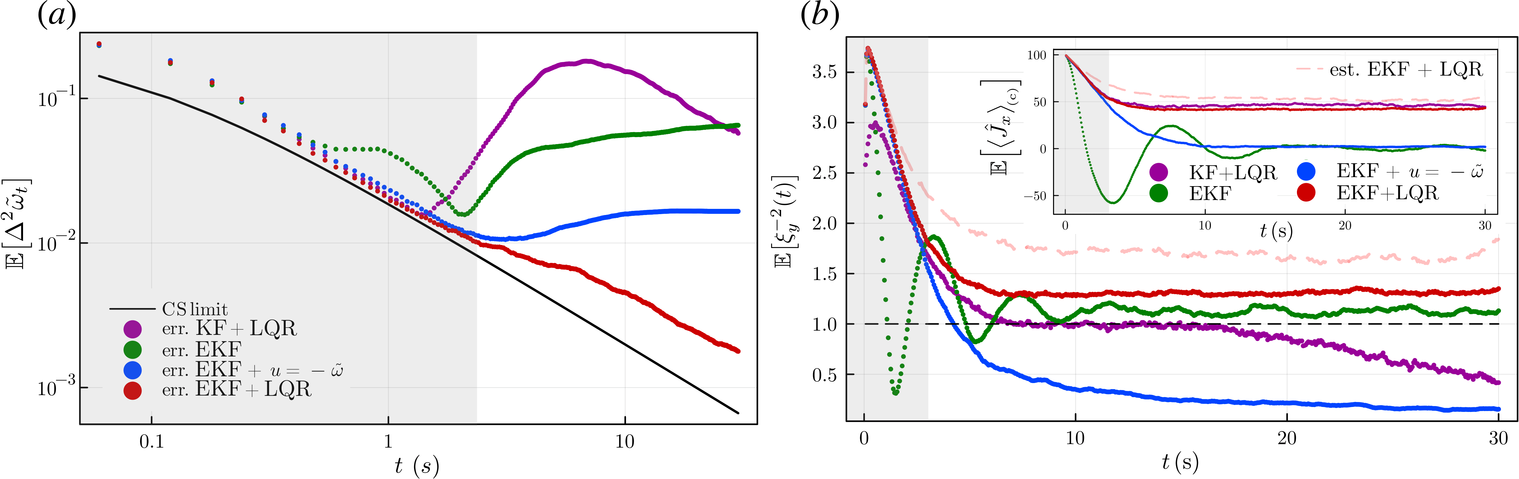
Figure 3: Performance of different estimation and control strategies. Subplot (a) presents the evolution of the estimation error (aMSE) for different estimation+control strategies that involve either KF (purple) or EKF (all other) as estimators, and either none (green), field compensation (blue) or LQR (red) as feedback methods. These strategies are compared against the CS limit (black), which sets the ultimate bound on the attainable error. The EKF+LQR strategy outperforms all other schemes and maintains a decreasing error trend even beyond the LG regime (shaded grey area). Subplot (b) shows the dynamics of the spin-squeezing parameter (8) for all estimation+control strategies, while its inset depicts the corresponding evolutions of the spin-polarisation $\langle\hat{J}_{x}\rangle$ (all with consistent colouring). For the EKF+LQR strategy, both include also the values predicted by the EKF (pink dashed line), which are overoptimistic. The parameters used in the SME (2) for simulations are: $N=200$, $\kappa_{\mathrm{coll}}=0.02$, $\kappa_{\mathrm{loc}}=0$, $M=0.3$, $\omega=1$ and $\eta=1$. The KF and EKF estimators are initialised with the mean $\tilde{\boldsymbol{x}}(0)=(N/2,0,0,N/4,N/4,0,\mu_{0})^{\mathsf{T}}$ and covariance $\Sigma(0)=\mathrm{diag}\!\left(0,0,0,0,0,0,\sigma_{0}^{2}\right)$ dictated by the initial CCS state of the atoms, and the Gaussian prior distribution for $\omega\sim\mathcal{N}(\mu_{0},\sigma_{0}^{2})$. All results are obtained after averaging over $\nu=1000$ measurement trajectories, whereas $\omega$-averaging is avoided by choosing its true value $\omega=1$ for a prior with $\mu_{0}=\omega+\sigma_{0}=1.5$ and $\sigma_{0}=0.5$.

Crucially, thanks to the dynamics (15) being linear, the LQR minimising Eq. (16) can be generally found by ignoring the stochastic part $\boldsymbol{\xi}$ in Eq. (15), which only increases the attainable minimal cost (16) (on average) [37]. Moreover, given also a linear observation model, e.g. Eq. (12), the optimal control problem can be solved independently to the state estimation task [37]. In particular, the LQR solution is then given by:

$$u(t) =-K_{C}\,\tilde{\boldsymbol{z}}(t),$$ (18)

$$K_{C} \coloneqq V^{-1}B^{\mathsf{T}}\Sigma_{C},$$ (19)

$$0 =A^{\mathsf{T}}\Sigma_{C}+\Sigma_{C}A+P-\Sigma_{C}BV^{-1}B^{\mathsf{T}}\Sigma_{C}$$ (20)

where the optimal control field $u(t)$ is linearly related at any time to the state estimator, $\tilde{\boldsymbol{z}}(t)$ (i.e. the KF for state (15) and observation (12) dynamics), by the gain (matrix) $K_{C}$. The gain is defined in Eq. (19) and involves the solution of the algebraic Riccati equation (20) for the matrix $\Sigma_{C}$. Now, as the matrices $A$ and $B$ in Eq. (15) are time-independent, all $\Sigma_{C}$, $K_{C}$, as well as the LQR, can be determined analytically [31]. In particular, the LQR in our case reads

$$u(t)=-\tilde{\omega}(t)-\lambda\;\big{\langle}\tilde{\hat{J}}_{y}(t)\big{\rangle}_{\!\scriptscriptstyle\mathrm{(c)}},$$ (21)

where $\lambda\coloneqq\sqrt{p_{J}/\nu}$ is a constant parameter that should be appropriately chosen. Note that by letting $\lambda=0$ we recover the (naive) field compensation strategy.

Furthermore, as in what follows we will use the LQR (21) also beyond the LG regime—in particular, in the CoG regime in which the EKF is used to estimate the full state $\boldsymbol{x}(t)=(\big{\langle}\hat{J}_{x}\big{\rangle}_{\!\scriptscriptstyle\mathrm{(c)}},\big{\langle}\hat{J}_{y}\big{\rangle}_{\!\scriptscriptstyle\mathrm{(c)}},\mathrm{V}_{x}^{\scriptscriptstyle\mathrm{(c)}},\mathrm{V}_{y}^{\scriptscriptstyle\mathrm{(c)}},\mathrm{V}_{z}^{\scriptscriptstyle\mathrm{(c)}},\mathrm{C}_{xy}^{\scriptscriptstyle\mathrm{(c)}},\omega)^{\mathsf{T}}$—we generalise the control law (18) to read $u(t)=-K_{C}\,\Xi\,\tilde{\boldsymbol{x}}(t)$, where $\Xi\coloneqq(0,1,0,\dots,0,0;0,0,0\dots,0,1)$ just selects the relevant state components of $\boldsymbol{x}(t)$ that appear in $\boldsymbol{z}(t)$, while $\tilde{\boldsymbol{x}}(t)$ is now the EKF estimator in Eq. (13a).

VI Real-time sensing performance

We benchmark the performance of the EKF+LQR strategy, on one hand, by demonstrating its superiority over other estimation+control strategies that involve less sophisticated inference (KF rather than EKF) and feedback (field compensation rather than LQR) methods. On the other, we verify whether and at what time-scales the CS limit (10) (induced by the global and/or local decoherence) can be attained—proving then the complete sensing scheme to be optimal, i.e., being optimised over not only the estimation+control strategy, but also the initial atomic state and any measurements involved.

In order to do so, we focus on identifying the evolution in time of the aMSE (5), $\mathbb{E}\!\left[{\Delta^{2}\tilde{\omega}_{t}}\right]$, see e.g. Fig. 3(a). However, in order to simultaneously monitor the dynamics of quantum correlations and coherence exhibited by the atomic ensemble, we also investigate the evolution of the spin-squeezing parameter (8), $\mathbb{E}\!\left[{\xi^{-2}_{y}(t)}\right]$, as well as the ensemble polarisation, $\mathbb{E}\!\left[{\big{\langle}\hat{J}_{x}\big{\rangle}_{\!\scriptscriptstyle\mathrm{(c)}}}\right]$, see the main and inset plots in Fig. 3(b), respectively.

Importantly, as the performance must be quantified on average, all the three quantities have to be averaged, $\mathbb{E}\!\left[{\cdot}\right]$, over sufficiently many measurement trajectories obtained when simulating the dynamics . Furthermore, the aMSE (5) must be averaged over the prior distribution $p(\omega)$, which represents our a priori knowledge about the Larmor frequency. However, in order to reduce the number of trajectories computed and improve the clarity of the presented plots, we avoid averaging over $p(\omega)$, but rather present measurement-trajectory averages for a fixed parameter value that is representative of the assumed prior, i.e. for $\omega=\mu\pm\sigma_{0}$ given a Gaussian prior $p(\omega)=\mathcal{N}(\mu_{0},\sigma_{0}^{2})$. For such an educated choice, the aMSE is consistently always greater than the CS limit (10) evaluated for the given $\sigma_{0}>0$, see e.g. Fig. 3(a), that, however, is always valid on average .

In what follows, we firstly focus on relatively low atomic numbers, $N$, for which we can explicitly simulate the true dynamics of the atomic ensemble along a particular measurement trajectory, as described in Sec. III.1. This allows us to demonstrate the superiority of the EKF+LQR strategy without making any approximations. However, as we observe and confirm, see App. F, that with an increase of $N$ the evolution of atoms can be well-described at short timescales by the CoG approximation of Sec. III.2, we then use it not only to construct the EKF but also for simulations. As a result, we are able to consider experimentally relevant numbers of atoms, e.g. $N=10^{5}$ [64, 65] used in Fig. 4, for which we may in detail demonstrate the optimality of EKF+LQR strategy by saturating the CS limit (10). What is more, we show large spin-squeezing to be then generated and long maintained despite decoherence—also for the unconditional dynamics thanks to the feedback (LQR), i.e. when averaging over the measurement trajectories.

VI.1 Identifying the best estimation and control strategy

In Fig. 3(a) we first compare the aMSE of the frequency estimate for four different estimation+control strategies when only the collective decoherence is present ($\kappa_{\mathrm{coll}}>0$, $\kappa_{\mathrm{loc}}=0$). This allows us to consider also the simplest estimation strategy based on the KF and linearised dynamics (15) [30, 35], which is not applicable as soon as $\kappa_{\mathrm{loc}}>0$ in Eq. (4). In particular, we compare: EKF with no control (in green), EKF with field compensation (denoted by $u(t)=-\tilde{\omega}(t)$, in blue), EKF+LQR ($u(t)$ as in Eq. (21) with $\lambda=1$, in red), and the (linearised) KF combined with LQR (in purple). As evident from Fig. 3(a), the EKF+LQR approach consistently outperforms all other strategies. Moreover, the results highlight the importance of using an estimator (EKF) that can handle non-linearities in the system, rather than a linear one (KF). Additionally, they stress the necessity of devising an appropriate feedback strategy following the principles of the LQR optimal-control theory.

Additional figures are presented in Fig. 3(b), in order to show that the EKF+LQR strategy (red) is the only one that keeps the ensemble both spin-squeezed and polarised along $x$ (main and inset, respectively) significantly beyond the LG regime ($t\!\lesssim\!(M+\kappa_{\mathrm{coll}})^{-1}$ [35], shaded in grey). When no control is applied (green), the atomic state is still squeezed on average ($\mathbb{E}\!\left[{\xi_{y}^{-2}(t)}\right]>1$) but quickly depolarises with the precession. When attempting to cancel the precession with just the estimate of the frequency, $u=-\tilde{\omega}$ (blue), both the polarisation and spin-squeezing (8) are rapidly lost. Controlling the sensor with an EKF+LQR instead of using $u=-\tilde{\omega}$ achieves an ideal outcome, preserving both spin-squeezing and polarisation well past the coherence time $1/\kappa_{\mathrm{coll}}$ at about $\mathbb{E}\!\left[{\xi_{y}^{-2}}\right]\approx 1.25$(0.97dB), and extending all the way to $t=30$, as shown in Fig. 3(b). Correct estimation is also crucial; employing a KF (purple) instead of an EKF, even combined with the best feedback strategy (LQR), results in a worse performance in terms of spin-squeezing, although polarisation is maintained.

VI.1.1 Using EKF to estimate spin-squeezing

A key advantage of using Kalman filtering techniques, or more generally Bayesian inference [55], over, e.g., model-free machine-learning methods [75, 76], is the fact that the former provide errors for their estimates, which are accurate as long as the dynamical model can be trusted. As noted in Sec. V.1, this is the case for the KF when LG stochastic models are considered, for which the KF’s covariance is assured to represent the true average error, i.e. $\Sigma(t)=\mathbb{E}\!\left[{\Delta^{2}\tilde{\boldsymbol{x}}(t)}\right]$ [38, 37]. For quantum LG models without feedback, the KF can thus be directly used to reconstruct conditional dynamics of any (Gaussian) quantum observable $\hat{X}(t)$ [19], even when only the unconditional dynamics is available due to, e.g., the model of measurement back-action being unknown [12].

In our case, to have only access to the unconditional dynamics of the system would mean having an unconditional evolution dictated by Eq. (2) without any feedback (since $u(t)$ is trajectory-dependent, i.e. $u(t)\equiv u(t|\boldsymbol{y}_{\leq t})$) and with the last $dW$-dependent term dropped. Then, the term $\big{\langle}\hat{J}_{y}(t)\big{\rangle}_{\!\scriptscriptstyle\mathrm{(c)}}$ in the detection model (1) should be reinterpreted as $J_{y}(t)\sim\mathcal{N}(\langle\hat{J}_{y}(t)\rangle,\Delta^{2}\hat{J}_{y}(t))$, so that it represents the particular value of $\hat{J}_{y}(t)$ occurring at time $t$—being drawn from the corresponding unconditional (Gaussian) Wigner function.

For any such unconditional dynamics, as long as it is LG, after initialising the KF to $\tilde{x}(0)=\langle\hat{X}(0)\rangle$ and $\Sigma_{xx}(0)=\Delta^{2}\hat{X}(0)$, the KF directly provides us in real time with $\tilde{x}(t)=\big{\langle}\hat{X}(t)\big{\rangle}_{\!\scriptscriptstyle\mathrm{(c)}}$ and $\Sigma_{xx}(t)=\Delta^{2}_{\scriptscriptstyle\mathrm{(c)}}\hat{X}$ based on the measurement data being recorded , i.e. the mean and variance, respectively, of the conditional (Gaussian) Wigner function correctly describing $\hat{X}(t)$ given the measurement record [78, 79]. Hence, as covariances of the KF represent then conditional variances of quantum observables, these can be directly used to, e.g., certify entanglement in QND-based experiments [12].

In contrast, as we possess an explicit model of the conditional dynamics (2), its solution (in the Heisenberg picture) for any moment of a quantum observable already accounts correctly for the measurement record observed, which in turn allows us to incorporate feedback [45]. Such moments, in particular $\big{\langle}\hat{J}_{\alpha}(t)\big{\rangle}_{\!\scriptscriptstyle\mathrm{(c)}}$ and $\Delta^{2}_{\scriptscriptstyle\mathrm{(c)}}\hat{J}_{\alpha}(t)\equiv\mathrm{V}_{\alpha}^{\scriptscriptstyle\mathrm{(c)}}$, constitute then dynamical parameters that can be tracked in real time, in the same way as the Larmor frequency $\omega$. Thus, one should view the CoG model (4) as a non-linear approximation that captures the conditional evolution for the observables of interest (their means and variances), whereas the EKF is a tool to infer these in an efficient way with $\omega$ being estimated in parallel. As a result, in contrast to the KF discussed above, the EKF must be initialised with the estimates of $\big{\langle}\hat{\boldsymbol{J}\hskip 2.84544pt}_{\alpha}(0)\big{\rangle}_{\!\scriptscriptstyle\mathrm{(c)}}=\langle\hat{\boldsymbol{J}\hskip 2.84544pt}\rangle_{\textsc{css}}$ and $\Delta^{2}_{\scriptscriptstyle\mathrm{(c)}}\hat{\boldsymbol{J}\hskip 2.84544pt}_{\alpha}(0)\equiv\boldsymbol{\mathrm{V}}_{\alpha}^{\scriptscriptstyle\mathrm{(c)}}(0)=\boldsymbol{\mathrm{V}}^{\textsc{css}}$ being determined by the ones of the CSS state and known exactly with no errors, i.e. with the corresponding covariance elements of the EKF, $\Sigma_{OO}(0)=0$ for all $O\neq\omega$ in Eq. (14), initially set to zero [30].

Nonetheless, the EKF estimates of relevant quantum means and variances, if accurate, can be directly used to, e.g., predict the conditional spin-squeezing of the ensemble. Still, one should be careful with such a procedure, as the EKF may overestimate on average both the spin-squeezing parameter (8) and the ensemble polarisation, $\mathbb{E}\!\left[{\xi^{-2}_{y}(t)}\right]$ and $\mathbb{E}\!\left[{\big{\langle}\hat{J}_{x}\big{\rangle}_{\!\scriptscriptstyle\mathrm{(c)}}}\right]$, as shown with pink dashed lines in the main and the inset of in Fig. 3(b), respectively. This is a result of operating at low $N=200$ in Fig. 3, for which the CoG model (4) used to construct the EKF approximates well the dynamics (2) only at short timescales ($t\ll(M+\kappa_{\mathrm{coll}})^{-1})$. However, we show in what follows that for relevant sizes of atomic ensembles, e.g., $N=10^{5}$ in Fig. 4, as long as the CoG approximation (4) is valid, the estimates provided by the EKF correctly predict the spin-squeezing parameter (8) on average.

VI.1.2 Benchmarking against a classical strategy with a strong measurement

In order to complete the discussion about the role of continuous spin-squeezing and the necessity to generate entanglement in achieving the aMSEs shown in Fig. 3, we decide to further benchmark the real-time estimation+control strategies against a classical scenario in which no entanglement is generated. As an alternative we consider the scheme in which the experimenter, rather than continuously probing the atomic ensemble until a given time $t$, performs any possible strong measurement at $t$. In such a case, rather than following the conditional dynamics (4), the ensemble evolves undisturbed (following Eq. (4) with $M\to 0$) until it is destructively measured. As elaborated on in App. E, the aMSE within such a scheme can still be constrained by the Bayesian Cramér-Rao Bound (9) but with $\mathcal{F}[\cdot]$ being replaced by the Quantum Fisher Information (QFI) [80].

We demonstrate in App. E by resorting to exact numerical simulations for the real-time scenarios as above, and computing explicitly the relevant QFI for the classical scenario, that the classical limit is indeed surpassed by the EKF+LQR strategy despite the presence of relatively weak collective decoherence. Moreover, as within the classical strategy there is no mechanism to counteract the decoherence, its usage becomes pointless at longer times $t$, at which the atoms reach a steady state that ceases to be sensitive to any variations of the estimated Larmor frequency $\omega$. We show this effect explicitly in App. E by choosing either the collective or local decoherence to be relatively strong, in order to stress that for the EKF+LQR strategy—because the information about the estimated $\omega$ keeps growing over time as the ensemble stabilises in a metrologically useful state—the aMSE keeps decreasing over long timescales, while the classical strategy quickly becomes useless in a single-shot scenario.

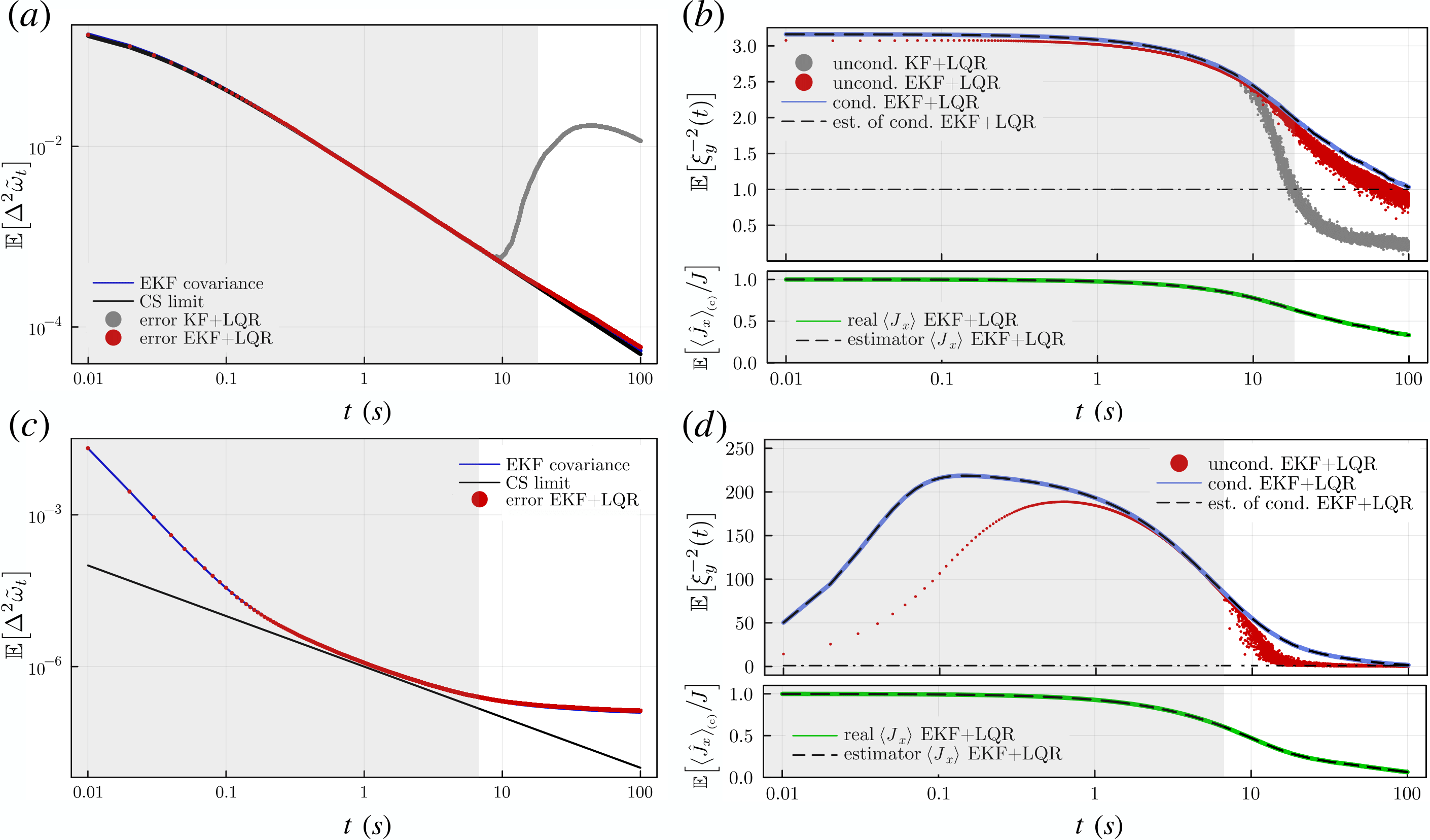
Figure 4: Performance in estimation and spin-squeezing extrapolated to large atomic ensembles, here $N=10^{5}$. Subplots (a) and (b) (upper row) depict the case of pure collective decoherence $\kappa_{\mathrm{coll}}=0.005$, whereas subplots (c) and (d) (lower row) deal with pure local decoherence $\kappa_{\mathrm{loc}}=0.05$. Left column: (a) and (c) show the error (aMSE) attained by the EKF+LQR strategy (red dots) when estimating $\omega$ and its average prediction by the EKF (blue line), $\mathbb{E}\!\left[{\Sigma_{\omega\omega}}\right]$, both being lower-bounded by the CS limit (10) (black line). For collective decoherence, the performance of KF+LQR strategy is also included (grey dots) to emphasise its failure beyond the LG regime (pink shading in all subplots). Right column: (b) and (d) illustrate the evolution of the spin-squeezing parameter (8) for conditional (blue line) and unconditional (red dots) dynamics, as compared with its classical threshold (horizontal dash-dotted line). The evolution of the ensemble polarisation $\langle\hat{J}_{x}\rangle=\mathbb{E}[\big{\langle}\hat{J}_{x}\big{\rangle}_{\!\scriptscriptstyle\mathrm{(c)}}]$ (green line) is also shown in both cases in extra lower plots. Both the conditional spin-squeezing and the polarisation in (b) and (d) are estimated very accurately by the EKF on average (superimposed dashed black lines). The above data is simulated employing the CoG model (4) with other parameters set to: $M=0.05$, $\omega=1$ and $\eta=1$. As in Fig. 3, the KF and EKF estimators are initialised with the mean $\tilde{\boldsymbol{x}}(0)=(N/2,0,0,N/4,N/4,0,\mu_{0})^{\mathsf{T}}$ and covariance $\Sigma(0)=\mathrm{diag}\!\left(0,0,0,0,0,0,\sigma_{0}^{2}\right)$ dictated by the initial CCS state and the Gaussian prior distribution for $\omega\sim\mathcal{N}(\mu_{0},\sigma_{0}^{2})$. All results are obtained after averaging over $\nu=20000$ measurement trajectories, while $\omega$-averaging is avoided by choosing the prior with $\sigma_{0}=0.5$ and $\mu_{0}=\omega+\sigma_{0}=1.5$.

VI.2 Extending the results to high $N$

As brute-force numerics become impossible, in order to extend the simulations of the dynamics (2) to high atomic numbers, $N$, we postulate that the CoG model (4) can be used not only within the EKF construction (13) but also to replace Eq. (2) when simulating the (conditional) dynamics of the first and second moments of the angular-momentum operators, while incorporating feedback. In App. F, by direct comparison with the exact solution of the SME (2), we show that with an increase in $N$ the CoG model predicts increasingly better both the polarisation $\big{\langle}\hat{J}_{x}\big{\rangle}_{\!\scriptscriptstyle\mathrm{(c)}}$ and the variance $\mathrm{V}_{y}^{\scriptscriptstyle\mathrm{(c)}}$ of the atomic ensemble that specify the spin-squeezing parameter (8), as long as the LG regime ($t\lesssim(M\!+\!2\kappa_{\mathrm{loc}}\!+\!\kappa_{\mathrm{coll}})^{-1}$) is considered. Moreover, if particularly the task of Larmor frequency estimation for the EKF+LQR scheme is of interest, the CoG model can be used for simulations far beyond the coherence time ($t\gtrsim(M\!+\!2\kappa_{\mathrm{loc}}\!+\!\kappa_{\mathrm{coll}})^{-1}$) unless significant collective decoherence ($\kappa_{\mathrm{coll}}>0$) is present, which makes the CoG model mildly but persistently inaccurate (below 1% of rel. error) despite the increasing $N$, see App. F.

In Fig. 4, we present the so-extrapolated results for $N=10^{5}$ (c.f. [64, 65]) to show explicitly that, for such a sufficiently large atomic number, the EKF+LQR strategy can be considered optimal within the LG regime, as its corresponding aMSE (in red) attains the CS limit (10) (in black) for both collective and local decoherence, see plots (a) and (c) of Fig. 4, respectively. Furthermore, it provides estimates of $\omega$ that improve with time also for timescales beyond the LG regime, $t>(M\!+\!2\kappa_{\mathrm{loc}}\!+\!\kappa_{\mathrm{coll}})^{-1}$, at which the KF+LQR strategy would fail, see the grey line in Fig. 4(a), or would not be even applicable in (c).

Strikingly, in both Fig. 4(a) and (c), i.e. both for collective and local decoherence, the average covariance of the EKF (in blue), $\mathbb{E}\!\left[{\Sigma_{\omega\omega}}\right]$, follows the true aMSE (in red). This confirms that, despite the nonlinearity of the CoG model (4), the (trajectory-dependent) error provided by the EKF can be trusted. In particular, the covariance provided by the EKF along any measurement trajectory correctly predicts the aMSE in the LG regime. Moreover, at longer timescales, it does not fluctuate significantly and concentrates onto the aMSE upon averaging over only a small number of repetitions.

Not only is the CS limit (10) not guaranteed to be generally tight but also for the local decoherence it diminishes as $\propto 1/N$, making its attainability even less likely. Still, as shown in Fig. 4(c), the aMSE of the EKF+LQR strategy (in red), superimposed on the EKF covariance (in blue), attains the CS limit (in black) for a short time window, so that its optimality can then be guaranteed—answering positively the open question posed in Ref. [36].

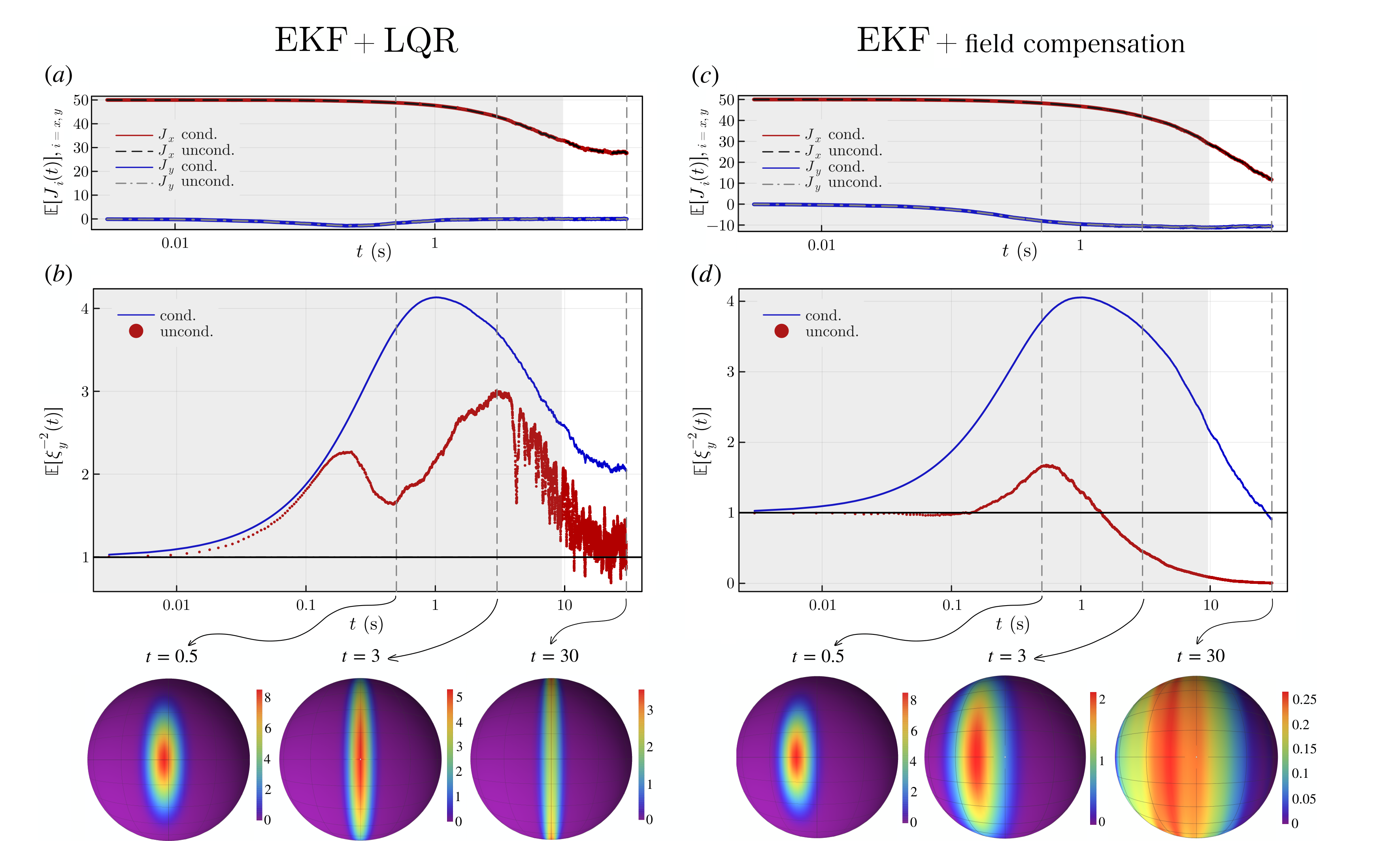
Figure 5: Conditional v.s. unconditional spin-squeezing. The exact ($N=100$) spin-squeezing dynamics with collective decoherence is shown depending on the control strategy: LQR (left column) vs (naive) field compensation (right column). Top row: Subplots (a) and (c) depict evolution of angular momentum components in $\hat{J}_{x}$ (red) and $\hat{J}_{y}$ (blue) directions, in particular their conditional and unconditional means that consistently match. Middle row: Subplots (b) and (d) compare the dynamics of the average unconditional (in red) and conditional (in blue) spin-squeezing parameters (8), also verifying whether they surpass the classical value (horizontal black line). Vertical dashed grey lines mark the relevant times for which we explicitly plot the spherical Wigner functions (bottom row) representing the instantaneous unconditional state. Note that for the LQR control (left), even though the width along $y$ of the distribution progressively narrows with time, the amplitude of the Wigner function also decays. The other parameters used in the SME (2) for simulations read: $\kappa_{\mathrm{coll}}=0.005$, $\kappa_{\mathrm{loc}}=0$, $M=0.1$, $\omega=1$, $\eta=1$. The EKF is initialised with the mean $\tilde{\boldsymbol{x}}(0)=(N/2,0,0,N/4,N/4,0,\mu_{0})^{\mathsf{T}}$ and covariance $\Sigma(0)=\mathrm{diag}\!\left(0,0,0,0,0,0,\sigma_{0}^{2}\right)$ dictated by the initial CCS state, and the Gaussian prior distribution for $\omega\sim\mathcal{N}(\mu_{0},\sigma_{0}^{2})$. All results are obtained after averaging over $\nu=500$ measurement trajectories, while $\omega$-averaging is avoided by choosing the prior with $\sigma_{0}=0.5$ and $\mu_{0}=\omega+\sigma_{0}=1.5$.

VII Conditional v.s. unconditional Spin Squeezing

When discussing spin-squeezing results, we can either focus on the spin-squeezing parameter (8) evaluated along a specific measurement trajectory (i.e. conditional), relevant for real-time magnetometry, or examine the entire feedback loop system as a mechanism for generating an entangled state independent of our observations (i.e. unconditional). While the conditional state of the system $\rho_{\scriptscriptstyle\mathrm{(c)}}(t)\equiv\rho(t|\boldsymbol{y}_{\leq t})$ is understood as the one most closely describing the state given a particular measurement record $\boldsymbol{y}_{\leq t}$, an unconditional state $\rho(t)$ describes the system when we discard, or do not have access to, the measurement outcomes, what formally corresponds to averaging the conditional state over all the possible past measurement trajectories, i.e. $\rho(t)=\mathbb{E}_{p(\boldsymbol{y}_{\leq t})}\!\left[\rho_{\scriptscriptstyle\mathrm{(c)}}(t)\right]$.

In the absence of feedback, the impact that continuously measuring the system has on the unconditional dynamics of $\rho(t)$ is simply to introduce extra collective decoherence—e.g. in case of the SME (2) with $u(t)=0$ after taking $\mathbb{E}_{p(\boldsymbol{y}_{\leq t})}\!\left[\cdot\right]$ of both sides, the measurement induces only the extra $M\mathcal{D}[\hat{J}_{y}]$-term. On the contrary, in the presence of feedback, the effective master equation describing the unconditional evolution cannot be easily deduced from the conditional dynamics, e.g. from Eq. (2), unless restrictive assumptions (e.g. Markovianity) are made [27], which are not fulfilled for the LQR-based control strategy described in Sec. V.2. However, as such restrictive feedback scenarios are known to unconditionally drive the system into a spin-squeezed state [70, 71], we confirm that this is also the case here.

In subplots (b) and (d) of Fig. 4, we demonstrate that the EKF+LQR strategy is not only capable to generate conditional spin-squeezing (blue lines), as already shown in Fig. 3(b) for $N=200$, but also yields significant unconditional spin-squeezing (red dots) above the classical limit (horizontal solid black line). Furthermore, as Fig. 4 presents extrapolated results using the CoG model (4) for $N=10^{5}$, thanks to dealing with a large atomic ensemble the EKF estimates very accurately both the average conditional spin-squeezing parameter (8) and the polarization, i.e. in Fig. 4(b&d) the dashed black lines coincide with the blue and green lines, respectively—in contrast to previously considered Fig. 3(b) and its inset, with pink dashed lines largely overestimating both the spin-squeezing parameter and the polarisation. While Fig. 4(b) highlights the advantages of using the EKF over the KF (grey dots) for maintaining the multi-particle entangled state beyond the LG regime—the unconditional spin-squeezing is lost at timescales $\sim\!10$ times shorter for the KF—the reliability of these conclusions is compromised by the limitations of the CoG approximation at long times, see App. F.

That is why, we return in Fig. 5 to simulating the exact SME (2) in the presence of only the collective decoherence ($N=100$, $\kappa_{\mathrm{coll}}=0.005$), where we study in detail the phenomenon of conditional vs. unconditional spin-squeezing by comparing further the EKF+LQR strategy (left column) with the naive field compensation (right column). Similarly to Fig. 4(b&d), we present in Fig. 5(b&d) the average conditional spin-squeezing parameter (blue) in comparison with the unconditional spin-squeezing of the average state (red), of which the latter also breaches the classical value (solid black horizontal line) beyond the LG regime for the EKF+LQR strategy employed in Fig. 5(b). This is confirmed by the (spherical) Wigner distribution plots (snapshots in time at $t=0.5,3,30$), which for the EKF+LQR strategy are clearly steadily “squeezed” in the $y$-direction even at $t=30\,>\,1/(M+\kappa_{\mathrm{coll}})\approx 10$, in contrast to the field-compensation strategy in which case the Wigner distribution begins to lose its shape already at $t=3$ within the LQ regime.

As the $\omega$-estimate of the EKF is initially set in Fig. 5 to $\tilde{\omega}(0)>\omega$, the control operation initially overcompensates for the Larmor precession and rotates the spin in the counter-clockwise direction when viewed along $z$—this is manifested by the spin components $\langle\hat{J}_{y}\rangle=\mathbb{E}[\big{\langle}\hat{J}_{y}\big{\rangle}_{\!\scriptscriptstyle\mathrm{(c)}}]$ acquiring negative values in both (a) and (c), as well as by the corresponding Wigner function being shifted to the left, e.g. at $t=0.5$ for both control strategies. An analogous behaviour would occur when choosing $\tilde{\omega}(0)<\omega$, in which case the control operation would initially undercompensate the Larmor precession, so that the spin rotates clockwise around $z$ (Wigner function shifts to the right), before either the LQR control increases the counter-rotation and stabilises the spin along $x$ (left column) or the stability is lost when the naive field-compensation strategy is pursued (right column).

VIII Conclusions

In this study, the dynamics and precision limits of atomic sensors for real-time magnetic field detection were investigated; first by exact numerical simulation of the system and later by introducing a co-moving Gaussian approximation suitable for large atomic (spin-$1/2$) ensembles. A significant contribution of our work is to explicitly incorporate measurement-based feedback schemes into the dynamical description of the atomic ensemble, which simultaneously experiences both local and collective decoherence in the form of dephasing along the magnetic-field direction.

In particular, having access to an effective Gaussian description, we propose a scheme that involves the so-called Extended Kalman Filter (EKF) and Linear Quadratic Regulator (LQR) to perform estimation and control, respectively. In parallel, we derive general bounds on the attainable precision induced by the decoherence, which apply to any strategy potentially involving a measurement-based feedback mechanism. This allows us to prove the EKF+LQR scheme to be optimal at short timescales. Moreover, the estimation error so-attained keeps decreasing over longer times—manifesting the stability of our control solution. This is enhanced by the fact that the atoms exhibit entanglement not only along a particular measurement trajectory (conditional spin-squeezing) but also, thanks to the LQR-control, when the measurement outcomes are discarded (unconditional spin-squeezing). Furthermore, for large atomic ensembles with $N\gtrsim 10^{5}$, the EKF correctly predicts the average error with which it estimates the Larmor frequency. Moreover, it naturally provides estimates of the angular-momentum means and variances, and hence allows to infer directly the conditional spin-squeezing in real time.

Our work demonstrates for the first time that practical measurement-based feedback schemes can significantly enhance the operation of atomic sensors by exploiting quantum entanglement despite the noise. As a result, we believe that it paves the way for such schemes to be employed in the state-of-the-art atomic magnetometers.

Appendix A Wigner function on a sphere

State representations on the Bloch sphere are useful to visualise spin-squeezing for an ensemble of (spin-$1/2$) atoms, and to gain intuition about properties of the overall quantum state. For that reason, we choose to compute the Wigner quasiprobability distribution and map it into the Bloch sphere as described in Ref. [40], i.e.:

$$W(\theta,\phi)=\sqrt{\frac{N+1}{4\pi}}\sum_{k=0}^{N}\sum_{q=-k}^{k}\rho_{kq}Y_{kq}(\theta,\phi)$$ (22)

where $Y_{kq}(\theta,\phi)$ are the complex spherical harmonics, for which the coefficients $\rho_{kq}=\sum_{m_{1},m_{2}=-J}^{J}\rho_{m_{1},m_{2}}t_{kq}^{m_{1}m_{2}}$ are determined by the part of the density matrix supported by the totally symmetric subspace, in particular, its elements $\rho_{m_{1},m_{2}}$ written in the angular momentum basis for the maximal total spin $J=N/2$, with the Clebsch-Gordan coefficients being $t_{kq}^{m_{1}m_{2}}\coloneqq(-1)^{J-m_{1}-q}\langle J,m_{1};J,-m_{2}|k,q\rangle$ [81, 82]. Note that the exact density matrix is needed to generate the Wigner quasiprobability distribution (22), therefore only in the case where we can solve the SME (2) exactly ($N\lesssim 300$), we may compute $W(\theta,\phi)$.

Throughout the manuscript we present Wigner functions mapped onto Bloch spheres to illustrate the distribution of coherent spin states (e.g. in Fig. 2), or to show how the EKF+LQR (estimation+control) strategy unconditionally squeezes the atomic ensemble (in Fig. 5) despite collective decoherence. Note that in presence of local decoherence the state is no longer supported only by the totally symmetric subspace, so that $W(\theta,\phi)$ no longer captures all its properties.

Appendix B Derivation of the CoG dynamical model (4)

The set of stochastic differential equations (4) can be derived by carefully applying the rules of Itô calculus, e.g., by noting that the differential of any two functions of time and a stochastic process, $f$ and $g$, reads $d(fg)=fdg+gdf+dfdg$. In our case, these functions are the means, variances and covariances of some quantum observable $\hat{O}$, whose dynamical evolution can then be computed by substituting the conditional dynamics (2) of $d\rho_{\scriptscriptstyle\mathrm{(c)}}$ into $d\langle\hat{O}\rangle=\mathrm{Tr}\{\hat{O}\,d\rho_{\scriptscriptstyle\mathrm{(c)}}\}$. In particular, considering $\hat{J}_{\alpha}$, $\mathrm{V}^{\scriptscriptstyle\mathrm{(c)}}_{\alpha}$ and $\mathrm{C}^{\scriptscriptstyle\mathrm{(c)}}_{\alpha\beta}$ with $\alpha,\beta=x,y,z$ appearing in Eq. (4), which satisfy

$$d\big{\langle}\hat{J}_{\alpha}\big{\rangle}_{\!\scriptscriptstyle\mathrm{(c)}}=\mathrm{Tr}[\hat{J}_{\alpha}\,d\rho_{\scriptscriptstyle\mathrm{(c)}}]$$ (23a)

$$d\mathrm{V}^{\scriptscriptstyle\mathrm{(c)}}_{\alpha}=d\big{\langle}\hat{J}_{\alpha}^{2}\big{\rangle}_{\!\scriptscriptstyle\mathrm{(c)}}-d(\big{\langle}\hat{J}_{\alpha}\big{\rangle}_{\!\scriptscriptstyle\mathrm{(c)}}^{2})$$ (23b)

$$\qquad\,=d\big{\langle}\hat{J}_{\alpha}^{2}\big{\rangle}_{\!\scriptscriptstyle\mathrm{(c)}}-2\big{\langle}\hat{J}_{\alpha}\big{\rangle}_{\!\scriptscriptstyle\mathrm{(c)}}d(\big{\langle}\hat{J}_{\alpha}\big{\rangle}_{\!\scriptscriptstyle\mathrm{(c)}})-d\big{\langle}\hat{J}_{\alpha}\big{\rangle}_{\!\scriptscriptstyle\mathrm{(c)}}d\big{\langle}\hat{J}_{\alpha}\big{\rangle}_{\!\scriptscriptstyle\mathrm{(c)}}$$

$$d\mathrm{C}^{\scriptscriptstyle\mathrm{(c)}}_{\alpha\beta}=\frac{1}{2}d\big{\langle}\hat{J}_{\alpha}\hat{J}_{\beta}\big{\rangle}_{\!\scriptscriptstyle\mathrm{(c)}}+\frac{1}{2}d\big{\langle}\hat{J}_{\beta}\hat{J}_{\alpha}\big{\rangle}_{\!\scriptscriptstyle\mathrm{(c)}}-d(\big{\langle}\hat{J}_{\alpha}\big{\rangle}_{\!\scriptscriptstyle\mathrm{(c)}}\big{\langle}\hat{J}_{\beta}\big{\rangle}_{\!\scriptscriptstyle\mathrm{(c)}})$$

$$\qquad\;=\frac{1}{2}d\big{\langle}\hat{J}_{\alpha}\hat{J}_{\beta}\big{\rangle}_{\!\scriptscriptstyle\mathrm{(c)}}+\frac{1}{2}d\big{\langle}\hat{J}_{\beta}\hat{J}_{\alpha}\big{\rangle}_{\!\scriptscriptstyle\mathrm{(c)}}-\big{\langle}\hat{J}_{\beta}\big{\rangle}_{\!\scriptscriptstyle\mathrm{(c)}}d\big{\langle}\hat{J}_{\alpha}\big{\rangle}_{\!\scriptscriptstyle\mathrm{(c)}}$$

$$\qquad\qquad-\big{\langle}\hat{J}_{\alpha}\big{\rangle}_{\!\scriptscriptstyle\mathrm{(c)}}d\big{\langle}\hat{J}_{\beta}\big{\rangle}_{\!\scriptscriptstyle\mathrm{(c)}}-d\big{\langle}\hat{J}_{\alpha}\big{\rangle}_{\!\scriptscriptstyle\mathrm{(c)}}d\big{\langle}\hat{J}_{\beta}\big{\rangle}_{\!\scriptscriptstyle\mathrm{(c)}},$$ (23c)

we derive by working to the relevant order $O(dt^{3/2})$:

$$d\big{\langle}\hat{J}_{x}\big{\rangle}_{\!\scriptscriptstyle\mathrm{(c)}}=-(\omega\!+\!u(t))\big{\langle}\hat{J}_{y}\big{\rangle}_{\!\scriptscriptstyle\mathrm{(c)}}dt\!-\frac{1}{2}(\kappa_{\mathrm{coll}}\!+\!2\kappa_{\mathrm{loc}}\!+\!M)\big{\langle}\hat{J}_{x}\big{\rangle}_{\!\scriptscriptstyle\mathrm{(c)}}dt\!+\!2\sqrt{\eta M}\mathrm{C}_{xy}^{\scriptscriptstyle\mathrm{(c)}}\,dW$$ (24a)

$$d\big{\langle}\hat{J}_{y}\big{\rangle}_{\!\scriptscriptstyle\mathrm{(c)}}=(\omega\!+\!u(t))\big{\langle}\hat{J}_{x}\big{\rangle}_{\!\scriptscriptstyle\mathrm{(c)}}dt\!-\frac{1}{2}(\kappa_{\mathrm{coll}}\!+\!2\kappa_{\mathrm{loc}})\big{\langle}\hat{J}_{y}\big{\rangle}_{\!\scriptscriptstyle\mathrm{(c)}}dt\!+\!2\sqrt{\eta M}\mathrm{V}_{y}^{\scriptscriptstyle\mathrm{(c)}}\,dW$$ (24b)

$$d\big{\langle}\hat{J}_{z}\big{\rangle}_{\!\scriptscriptstyle\mathrm{(c)}}=-\frac{1}{2}M\big{\langle}\hat{J}_{z}\big{\rangle}_{\!\scriptscriptstyle\mathrm{(c)}}dt\!+\!2\sqrt{\eta M}\mathrm{C}_{zy}^{\scriptscriptstyle\mathrm{(c)}}\,dW$$ (24c)

$$d\mathrm{V}_{x}^{\scriptscriptstyle\mathrm{(c)}}=-2(\omega\!+\!u(t))\mathrm{C}_{xy}^{\scriptscriptstyle\mathrm{(c)}}dt\!+\!\kappa_{\mathrm{coll}}\!\left(\!\mathrm{V}_{y}^{\scriptscriptstyle\mathrm{(c)}}\!+\!\big{\langle}\hat{J}_{y}\big{\rangle}_{\!\scriptscriptstyle\mathrm{(c)}}^{2}\!-\!\mathrm{V}_{x}^{\scriptscriptstyle\mathrm{(c)}}\!\right)\!dt\!+\!\kappa_{\mathrm{loc}}\!\left(\!\frac{N}{2}\!-\!2\mathrm{V}_{x}^{\scriptscriptstyle\mathrm{(c)}}\!\right)\!dt\!+\!M\!\left(\!\mathrm{V}_{z}^{\scriptscriptstyle\mathrm{(c)}}\!-\!\mathrm{V}_{x}^{\scriptscriptstyle\mathrm{(c)}}\!-\!4\eta{\mathrm{C}_{xy}^{\scriptscriptstyle\mathrm{(c)}}}^{2}\!\right)\!dt$$

$$\;\;\;\;\;\;\;\;\;\;\;\;+2\sqrt{\eta M}\left(\frac{1}{2}\mathrm{cov}_{\scriptscriptstyle\mathrm{(c)}}(\hat{J}_{x}^{2}\hat{J}_{y})+\frac{1}{2}\mathrm{cov}_{\scriptscriptstyle\mathrm{(c)}}(\hat{J}_{y}\hat{J}_{x}^{2})\right)dW$$ (24d)

$$d\mathrm{V}_{y}^{\scriptscriptstyle\mathrm{(c)}}=2(\omega\!+\!u(t))\mathrm{C}_{xy}^{\scriptscriptstyle\mathrm{(c)}}dt\!+\!\kappa_{\mathrm{coll}}\!\left(\!\mathrm{V}_{x}^{\scriptscriptstyle\mathrm{(c)}}\!+\!\big{\langle}\hat{J}_{x}\big{\rangle}_{\!\scriptscriptstyle\mathrm{(c)}}^{2}\!-\!\mathrm{V}_{y}^{\scriptscriptstyle\mathrm{(c)}}\!\right)\!dt\!+\!\kappa_{\mathrm{loc}}\!\left(\!\frac{N}{2}\!-\!2\mathrm{V}_{y}^{\scriptscriptstyle\mathrm{(c)}}\!\right)\!dt\!-\!4\eta M{\mathrm{V}_{y}^{\scriptscriptstyle\mathrm{(c)}}}^{2}dt$$

$$\;\;\;\;\;\;\;\;\;\;\;\,+2\sqrt{\eta M}\,\mathrm{cov}_{\scriptscriptstyle\mathrm{(c)}}(\hat{J}_{y}^{3})\,dW$$ (24e)

$$d\mathrm{V}_{z}^{\scriptscriptstyle\mathrm{(c)}}=M\!\left(\!\mathrm{V}_{x}^{\scriptscriptstyle\mathrm{(c)}}\!+\!\big{\langle}\hat{J}_{x}\big{\rangle}_{\!\scriptscriptstyle\mathrm{(c)}}^{2}\!-\!\mathrm{V}_{z}^{\scriptscriptstyle\mathrm{(c)}}\!\right)\!dt+2\sqrt{\eta M}\left(\frac{1}{2}\mathrm{cov}_{\scriptscriptstyle\mathrm{(c)}}(\hat{J}_{z}^{2}\hat{J}_{y})+\frac{1}{2}\mathrm{cov}_{\scriptscriptstyle\mathrm{(c)}}(\hat{J}_{y}\hat{J}_{z}^{2})\right)\,dW$$ (24f)

$$d\mathrm{C}_{xy}^{\scriptscriptstyle\mathrm{(c)}}=(\omega\!+\!u(t))\!\left(\!\mathrm{V}_{x}^{\scriptscriptstyle\mathrm{(c)}}\!-\!\mathrm{V}_{y}^{\scriptscriptstyle\mathrm{(c)}}\!\right)\!dt\!-\!\kappa_{\mathrm{coll}}\!\left(\!2\mathrm{C}_{xy}^{\scriptscriptstyle\mathrm{(c)}}\!+\!\big{\langle}\hat{J}_{x}\big{\rangle}_{\!\scriptscriptstyle\mathrm{(c)}}\big{\langle}\hat{J}_{y}\big{\rangle}_{\!\scriptscriptstyle\mathrm{(c)}}\!\right)\!dt\!-\!2\kappa_{\mathrm{loc}}\mathrm{C}_{xy}^{\scriptscriptstyle\mathrm{(c)}}dt\!-\!\frac{1}{2}M\mathrm{C}_{xy}^{\scriptscriptstyle\mathrm{(c)}}\left(1+8\eta\mathrm{V}_{y}^{\scriptscriptstyle\mathrm{(c)}}\right)\!dt$$

$$\;\;\;\;\;\;\;\;\;\;\;\;\;\;+2\sqrt{\eta M}\left(\frac{1}{4}\mathrm{cov}_{\scriptscriptstyle\mathrm{(c)}}(\hat{J}_{x}\hat{J}_{y}^{2})+\frac{1}{2}\mathrm{cov}_{\scriptscriptstyle\mathrm{(c)}}(\hat{J}_{y}\hat{J}_{x}\hat{J}_{y})+\frac{1}{4}\mathrm{cov}_{\scriptscriptstyle\mathrm{(c)}}(\hat{J}_{y}^{2}\hat{J}_{x})\right)dW$$ (24g)

$$d\mathrm{C}_{zy}^{\scriptscriptstyle\mathrm{(c)}}=(\omega\!+\!u(t))\mathrm{C}_{xz}^{\scriptscriptstyle\mathrm{(c)}}dt-\frac{1}{2}\left(\kappa_{\mathrm{coll}}+2\kappa_{\mathrm{loc}}+M\left(1+8\eta\mathrm{V}_{y}^{\scriptscriptstyle\mathrm{(c)}}\right)\right)\mathrm{C}_{zy}^{\scriptscriptstyle\mathrm{(c)}}dt$$ (24h)

$$\;\;\;\;\;\;\;\;\;\;\;\;\;\;+2\sqrt{\eta M}\bigg{(}\frac{1}{4}\mathrm{cov}_{\scriptscriptstyle\mathrm{(c)}}(\hat{J}_{z}\hat{J}_{y}^{2})+\frac{1}{2}\mathrm{cov}_{\scriptscriptstyle\mathrm{(c)}}(\hat{J}_{y}\hat{J}_{z}\hat{J}_{y})+\frac{1}{4}\mathrm{cov}_{\scriptscriptstyle\mathrm{(c)}}(\hat{J}_{y}^{2}\hat{J}_{z})\bigg{)}dW$$ (24i)

$$d\mathrm{C}_{xz}^{\scriptscriptstyle\mathrm{(c)}}=-(\omega\!+\!u(t))\mathrm{C}_{zy}^{\scriptscriptstyle\mathrm{(c)}}dt-\frac{1}{2}\left(\kappa_{\mathrm{coll}}+2\kappa_{\mathrm{loc}}+4M\right)\mathrm{C}_{xz}^{\scriptscriptstyle\mathrm{(c)}}dt-M\big{\langle}\hat{J}_{z}\big{\rangle}_{\!\scriptscriptstyle\mathrm{(c)}}\big{\langle}\hat{J}_{x}\big{\rangle}_{\!\scriptscriptstyle\mathrm{(c)}}dt-4\eta M\mathrm{C}_{xy}^{\scriptscriptstyle\mathrm{(c)}}\mathrm{C}_{zy}^{\scriptscriptstyle\mathrm{(c)}}dt$$ (24j)

$$\;\;\;\;\;\;\;\;\;\;\;\;\;\;+2\sqrt{\eta M}\bigg{(}\frac{1}{4}\mathrm{cov}_{\scriptscriptstyle\mathrm{(c)}}(\hat{J}_{x}\hat{J}_{z}\hat{J}_{y})+\frac{1}{4}\mathrm{cov}_{\scriptscriptstyle\mathrm{(c)}}(\hat{J}_{y}\hat{J}_{x}\hat{J}_{z})+\frac{1}{4}\mathrm{cov}_{\scriptscriptstyle\mathrm{(c)}}(\hat{J}_{z}\hat{J}_{x}\hat{J}_{y})+\frac{1}{4}\mathrm{cov}_{\scriptscriptstyle\mathrm{(c)}}(\hat{J}_{y}\hat{J}_{z}\hat{J}_{x})\bigg{)}dW$$ (24k)

where for any three operators $\hat{A}$, $\hat{B}$ and $\hat{C}$, we define

$$\mathrm{cov}_{\scriptscriptstyle\mathrm{(c)}}(\hat{A}\hat{B}\hat{C})\coloneqq\big{\langle}\hat{A}\hat{B}\hat{C}\big{\rangle}_{\!\scriptscriptstyle\mathrm{(c)}}-\big{\langle}\hat{A}\big{\rangle}_{\!\scriptscriptstyle\mathrm{(c)}}\big{\langle}\hat{B}\hat{C}\big{\rangle}_{\!\scriptscriptstyle\mathrm{(c)}}-\big{\langle}\hat{B}\big{\rangle}_{\!\scriptscriptstyle\mathrm{(c)}}\big{\langle}\hat{A}\hat{C}\big{\rangle}_{\!\scriptscriptstyle\mathrm{(c)}}-\big{\langle}\hat{C}\big{\rangle}_{\!\scriptscriptstyle\mathrm{(c)}}\big{\langle}\hat{A}\hat{B}\big{\rangle}_{\!\scriptscriptstyle\mathrm{(c)}}+2\big{\langle}\hat{A}\big{\rangle}_{\!\scriptscriptstyle\mathrm{(c)}}\big{\langle}\hat{B}\big{\rangle}_{\!\scriptscriptstyle\mathrm{(c)}}\big{\langle}\hat{C}\big{\rangle}_{\!\scriptscriptstyle\mathrm{(c)}}.$$ (25)

In order to be able to construct an EKF from the equations above, as well as to have a manageable system of stochastic differential equations that approximately describe our sensor, we drop the third order moments from Eq. (24), i.e., we perform a cut-off approximation. Crucially, third order moments appear only in the stochastic terms of the dynamical equations for the second order moments, reducing the impact of the approximation in the accuracy of the CoG model.

Additionally, in the main text we also omit the differential equations for $\big{\langle}\hat{J}_{z}\big{\rangle}_{\!\scriptscriptstyle\mathrm{(c)}}$, $\mathrm{C}_{xz}^{\scriptscriptstyle\mathrm{(c)}}$ or $\mathrm{C}_{zy}^{\scriptscriptstyle\mathrm{(c)}}$, since these quantities are consistently zero throughout the time evolution. This follows from their initial (CSS-state) conditions, i.e. $\langle\hat{J}_{z}(0)\rangle=\mathrm{C}_{xz}^{\scriptscriptstyle\mathrm{(c)}}(0)=\mathrm{C}_{zy}^{\scriptscriptstyle\mathrm{(c)}}(0)=0$, and their exclusively decaying evolution when the stochastic kicks due to the third-order moments are disregarded.

Appendix C Classical Simulation bound for local and global decoherence

Although the Larmor frequency $\omega$ maybe allowed to follow itself a stochastic process [41], here we focus on estimating its constant value by employing a Bayesian strategy. Within the Bayesian approach to estimation theory, the aMSE can be lower-bounded by different classes of Bayesian bounds [67]. For our purposes, we choose the (marginal unconditional) Bayesian Cramér-Rao Bound (BCRB) [83, 67]:

$$\mathbb{E}\!\left[{\Delta^{2}\tilde{\omega}_{t}}\right]\geq(J_{B})^{-1},$$ (26)

where $J_{B}$ is the Bayesian information (BI) [55],

$$J_{B}\coloneqq\mathbb{E}_{p(\omega,\boldsymbol{y}_{\leq t})}\!\left[\left(\partial_{\omega}\ln p(\omega,\boldsymbol{y}_{\leq t})\right)^{2}\right].$$ (27)

The BI can be split into two terms, $J_{B}=J_{P}+J_{M}$. The first term, $J_{P}$, represents the contribution of our prior knowledge about $\omega$,

$$J_{P}=\mathcal{F}[p(\omega)]\coloneqq\mathbb{E}_{p(\omega)}\!\left[\left(\partial_{\omega}\ln p(\omega)\right)^{2}\right],$$ (28)

corresponding to the Fisher information (FI) of the prior distribution $p(\omega)$ evaluated w.r.t. the estimated parameter $\omega$. As in this work we assume the a priori knowledge about $\omega$ to be described by a Gaussian distribution of mean $\mu$ and variance $\sigma^{2}$,

$$\omega\sim p(\omega)=\frac{1}{\sqrt{2\pi\sigma^{2}}}\mathrm{e}^{-\frac{(\omega-\mu)^{2}}{2\sigma^{2}}},$$ (29)

its FI corresponds to just the inverse of the variance, i.e.:

$$J_{P}=\frac{1}{\sigma^{2}}.$$ (30)

The second term, namely the contribution of the measurement record, or $J_{M}$, can be understood as averaging the FI of the likelihood over the prior distribution, i.e.:

$$J_{M} \coloneqq\mathbb{E}_{p(\omega,\boldsymbol{y}_{\leq t})}\!\left[\left(\partial_{\omega}\ln p(\boldsymbol{y}_{\leq t},\omega)\right)^{2}\right]$$ (31)

$$=\int d\omega\;p(\omega)\,\mathcal{F}[p(\boldsymbol{y}_{\leq t}|\omega)],$$ (32)

with

$$\mathcal{F}[p(\boldsymbol{y}_{\leq t}|\omega)]\coloneqq\mathbb{E}_{p(\boldsymbol{y}_{\leq t}|\omega)}\!\left[\left(\partial_{\omega}\ln p(\boldsymbol{y}_{\leq t}|\omega)\right)^{2}\right]$$ (33)

being the FI of $p(\boldsymbol{y}_{\leq t}|\omega)$ w.r.t. $\omega$, i.e. the likelihood of observing a measurement trajectory $\boldsymbol{y}_{\leq t}$ given that the true value of the Larmor frequency is $\omega$.

Now, as $J_{M}$, or equivalently $\mathcal{F}[p(\boldsymbol{y}_{\leq t}|\omega)]$, depends on a particular measurement strategy assumed, in what follows we focus on establishing a universal upper bound on $J_{M}$ that applies no matter the measurement sequence, incl. measurement-based feedback, and which stems from our previous work [35].

C.1 Discrete-time picture of a continuous measurement with measurement-based feedback

Any conditional dynamics involving a continuous measurement, such as the SME (2), is generally derived as a continuous-time limit (${\delta t}\to 0$) of a discretised evolution consisting of a sequence of completely positive and trace-preserving (CPTP) maps, $\Phi_{\delta t}$ of duration ${\delta t}$, that are interspersed by weak sequential measurements [44].

In fact, the continuous measurement record $\boldsymbol{y}_{\leq t}$ over time $t=k{\delta t}$ corresponds to the limiting case of a sequence of outcomes $\boldsymbol{y}_{k}=\{y_{1},\dots,y_{k}\}$ after letting $k\to\infty$ as ${\delta t}\to 0$. Moreover, in presence of measurement-based feedback the system dynamics after the $\ell$th, but before the $(\ell+1)$th, measurement may depend on all the previously recorded outcomes $\boldsymbol{y}_{\ell}$, so that we label the CPTP map applicable during this timestep as $\Phi_{\delta t}^{\boldsymbol{y}_{\ell}}$, which also encodes the estimated $\omega$.

As a result, we can most generally write the conditional state $\rho_{\scriptscriptstyle\mathrm{(c)}}\equiv\rho(t|\boldsymbol{y}_{\leq t})$ at time $t$ in the discrete-time picture, i.e. after $k$ steps of duration ${\delta t}$, as

$$\;\rho(t|\boldsymbol{y}_{k})=$$ (34)

$$\ =\frac{\hat{E}_{y_{k}}\Phi_{\delta t}^{\boldsymbol{y}_{k-1}}\!\!\left[\dots\hat{E}_{y_{2}}\Phi_{\delta t}^{\boldsymbol{y}_{1}}\!\!\left[\hat{E}_{y_{1}}\Phi_{\delta t}\!\left[\rho_{0}\right]\!\hat{E}_{y_{1}}^{\dagger}\right]\hat{E}_{y_{2}}^{\dagger}\dots\right]\!\!\hat{E}_{y_{k}}^{\dagger}}{p(\boldsymbol{y}_{k}|\omega)},$$

where the denominator above is the discretised version of likelihood appearing in Eq. (33), i.e.:

$$\;p(\boldsymbol{y}_{k}|\omega)=$$ (35)

$$=\mathrm{Tr}\!\left\{\hat{E}_{y_{k}}\Phi_{\delta t}^{\boldsymbol{y}_{k-1}}\!\!\left[\dots\hat{E}_{y_{2}}\Phi_{\delta t}^{\boldsymbol{y}_{1}}\!\!\left[\hat{E}_{y_{1}}\Phi_{\delta t}\!\left[\rho_{0}\right]\!\hat{E}_{y_{1}}^{\dagger}\right]\hat{E}_{y_{2}}^{\dagger}\dots\right]\!\!\hat{E}_{y_{k}}^{\dagger}\right\}.$$

In Eq. (34), $\{\hat{E}_{y_{\ell}}^{\dagger}\hat{E}_{y_{\ell}}\}_{y_{\ell}}$ with $\sum_{y_{\ell}}\hat{E}_{y_{\ell}}^{\dagger}\hat{E}_{y_{\ell}}=\mathds{1}$ constitute a positive operator-valued measure (POVM) representing the discretised continuous measurement. For simplicity and direct applicability to the SME (2), we assume that the measurement (POVM) to be same within the sequence, i.e. for all $\ell=1,2,\dots,k$. However, let us stress that such an assumption is unnecessary in the derivation of precision bounds that follows. In particular, our analysis also applies to schemes in which the type of measurement, e.g. from homodyne to photodetection and vice versa, is adaptively changed over the course of a single measurement trajectory.

Focussing on a single ${\delta t}$-step in Eq. (34), we may relate the consecutive conditional states as follows

$$\rho_{\scriptscriptstyle\mathrm{(c)}}((\ell+1){\delta t})=\frac{\hat{E}_{y_{\ell+1}}\Phi_{\delta t}^{\boldsymbol{y}_{\ell}}[\rho_{\scriptscriptstyle\mathrm{(c)}}(\ell{\delta t})]\hat{E}_{y_{\ell+1}}^{\dagger}}{\mathrm{Tr}\!\left\{\hat{E}_{y_{\ell+1}}^{\dagger}\hat{E}_{y_{\ell+1}}\Phi_{\delta t}^{\boldsymbol{y}_{\ell}}[\rho_{\scriptscriptstyle\mathrm{(c)}}(\ell{\delta t})]\right\}},$$ (36)

where we assume $\Phi_{\delta t}^{\boldsymbol{y}_{\ell}}$ to constitute a semigroup, i.e.:

$$\Phi_{\delta t}^{\boldsymbol{y}_{\ell}}=\mathrm{e}^{\mathcal{L}_{\boldsymbol{y}_{\ell}}{\delta t}}$$ (37)

with $\mathcal{L}_{\boldsymbol{y}_{\ell}}$ being an arbitrary Markovian dynamical generator of the Gorini-Kosakowski-Sudarshan-Lindblad (GKSL) form [84]. Although $\mathcal{L}_{\boldsymbol{y}_{\ell}}$ incorporates measurement-based feedback and thus may depend on all previous outcomes $\boldsymbol{y}_{\ell}$, it is importantly time-invariant over the duration ${\delta t}$ of each timestep in between measurements. Yet, as this does not force us to use the same feedback strategy in each ${\delta t}$-timestep (as long as it is Markovian), the precision bounds we derive in what follows will also account for schemes involving measurement-based feedback, whose type is adaptively changed over the course of a single measurement trajectory.

Within the continuous measurement framework [44], the Kraus operators of the $\ell$th measurement in Eq. (36), $\{\hat{E}_{y_{\ell}}\}_{y_{\ell}}$, are generally associated with an interaction of the system with a bosonic mode, $\hat{B}_{\ell}$ satisfying $[\hat{B}_{\ell},\hat{B}_{\ell^{\prime}}^{\dagger}]=\delta_{\ell\ell^{\prime}}$, that is subsequently measured, so that:

$$\hat{E}_{y_{\ell}}=\bra{y_{\ell}}\hat{U}_{{\delta t}}\ket{0},$$ (38)

where the bosonic mode is initialised in the vacuum state $\ket{0}$ before being projected onto the state $\ket{y_{\ell}}$ associated with a particular outcome, while the (weak) interaction is generated by the unitary operation [44, 85, 86]:

$$\hat{U}_{{\delta t}}=\exp\!\left\{\sqrt{M{\delta t}}\,\left(\hat{L\,}\!\otimes\hat{B}_{\ell}^{\dagger}-\hat{L\,}\!^{\dagger}\otimes\hat{B}_{\ell}\right)\right\},$$ (39)

with $M$ parametrising the strength of the continuous measurement and $\hat{L\,}\!$ denoting any system operator that is continuously probed.

Physically, by taking the limit ${\delta t}\to 0$ we arrive at the scenario in which the conditional state (34) describes the system (here, the atomic ensemble) undergoing Markovian dynamics that incorporates measurement-based feedback, while interacting with a bosonic field $\hat{B}_{t}$ (the probing light) such that $[\hat{B}_{t},\hat{B}_{t^{\prime}}^{\dagger}]=\delta(t-t^{\prime})$, which couples to an arbitrary system operator and is arbitrarily measured in a time-local manner. Although the precision bounds we derive in what follows allow in principle also for collective (time-non-local) measurements of the bosonic field, this would require reconsideration of the feedback schemes considered.

Crucially, Eq. (36) combined with Eqs. (37) and (38) allows us to demonstrate that no matter the form of the continuous measurement, i.e. the choice of (pointer) states $\ket{y_{\ell}}_{\ell}$ in Eq. (38), the dynamical generator $\mathcal{L}_{\boldsymbol{y}_{\ell}}$ will appear in the final stochastic master equation (e.g. in Eq. (2)) not affecting and not being affected by the presence of the continuous measurement as ${\delta t}\to 0$.

Focussing on the unnormalised state after the $\ell$th step, i.e. the numerator in Eq. (36), we rewrite it as

$$\tilde{\rho}_{\scriptscriptstyle\mathrm{(c)}}((\ell+1){\delta t})=\bra{y_{\ell+1}}\!\hat{U}_{{\delta t}}\!\ket{0}\,\Phi_{\delta t}^{\boldsymbol{y}_{\ell}}[\rho_{\scriptscriptstyle\mathrm{(c)}}(\ell{\delta t})]\,\bra{0}\!\hat{U}_{{\delta t}}^{\dagger}\!\ket{y_{\ell+1}}$$

$$\qquad={\delta t}\,\mathcal{L}_{\boldsymbol{y}_{\ell}}\rho_{\scriptscriptstyle\mathrm{(c)}}(\ell{\delta t})$$

$$\qquad+M{\delta t}\left(\bra{y_{\ell+1}}\hat{G}_{\ell}\ket{0}\rho_{\scriptscriptstyle\mathrm{(c)}}(\ell{\delta t})+\textrm{h.c.}\right)$$

$$\qquad+\sqrt{M{\delta t}}\left(\bra{y_{\ell+1}}\hat{G}_{\ell}\ket{0}\rho_{\scriptscriptstyle\mathrm{(c)}}(\ell{\delta t})\bra{0}\hat{G}_{\ell}^{\dagger}\ket{y_{\ell+1}}\right)$$

$$\qquad+\frac{M{\delta t}}{2}\left(\bra{y_{\ell+1}}\hat{G}_{\ell}^{2}\ket{0}\rho_{\scriptscriptstyle\mathrm{(c)}}(\ell{\delta t})+\textrm{h.c.}\right)$$

$$\qquad+O({\delta t}^{3/2}),$$ (40)

where we define $\hat{G}_{\ell}\coloneqq\hat{L\,}\!\otimes\hat{B}_{\ell}^{\dagger}-\hat{L\,}\!^{\dagger}\otimes\hat{B}_{\ell}$ as the effective non-Hermitian interaction Hamiltonian appearing in Eq. (39). Now, it should be clear from Eq. (40) that in the limit ${\delta t}\to 0$ no terms appear that involve both $\mathcal{L}_{\boldsymbol{y}_{\ell}}$ and the continuous measurement, as these must be $o(t^{3/2})$. This is a consequence of the crucial Markovianity (semigroup) assumption stated in Eq. (37).

C.1.1 Example: continuous homodyne detection

For completeness, let us show this explicitly for the case of homodyne detection [87, 85] that importantly encapsulates the SME (2) of our interest. In what follows, we largely stem from the derivation presented in Ref. [86].

With the aim to derive the resulting stochastic differential equation, we focus on a single timestep (36) that we now relabel as $[t,t+{\mathrm{d}t}]$ in the continuous-time limit:

$$\rho_{\scriptscriptstyle\mathrm{(c)}}(t\!+\!{\mathrm{d}t})=\frac{\hat{E}_{x}\Phi_{{\mathrm{d}t}}^{\boldsymbol{y}_{\leq t}}[\rho_{\scriptscriptstyle\mathrm{(c)}}(t)]\hat{E}_{x}^{\dagger}}{\mathrm{Tr}\!\left\{\hat{E}_{x}^{\dagger}\hat{E}_{x}\Phi_{{\mathrm{d}t}}^{\boldsymbol{y}_{\leq t}}[\rho_{\scriptscriptstyle\mathrm{(c)}}(t)]\right\}},$$ (41)

where in case of continuous homodyne detection $\hat{E}_{x}=\bra{x}\hat{U}_{{\mathrm{d}t}}\ket{0}$ as in Eq. (38), but with the bosonic field being now projected the eigenstate $\ket{x}$ of its quadrature operator $\hat{x}_{t}=(\hat{B}_{t}^{\dagger}+\hat{B}_{t})/\sqrt{2}$ [85].

Let us define for convenience the unnormalised conditional state at $t+{\mathrm{d}t}$ in Eq. (41) for the outcome $x$ being observed as

$$\tilde{\rho}_{\scriptscriptstyle\mathrm{(c)}}(t\!+\!{\mathrm{d}t})\coloneqq\bra{x}\hat{U}_{{\mathrm{d}t}}\!\left(\Phi_{{\mathrm{d}t}}^{\boldsymbol{y}_{\leq t}}[\rho_{\scriptscriptstyle\mathrm{(c)}}\!(t)]\otimes\ket{0}\!\!\bra{0}\right)\!\hat{U}_{{\mathrm{d}t}}^{\dagger}\ket{x},$$ (42)

with the probability of obtaining $x$ being then given by $p_{x}(t\!+\!{\mathrm{d}t})=\mathrm{Tr}\!\left\{\tilde{\rho}_{\scriptscriptstyle\mathrm{(c)}}(t\!+\!{\mathrm{d}t})\right\}$, which satisfies for ${\mathrm{d}t}=0$:

$$p_{x}(t) =\mathrm{Tr}\!\left\{\tilde{\rho}_{\scriptscriptstyle\mathrm{(c)}}(t)\right\}=\mathrm{Tr}\!\left\{\bra{x}\left(\rho_{\scriptscriptstyle\mathrm{(c)}}\!(t)\otimes\ket{0}\!\!\bra{0}\right)\ket{x}\right\}$$

$$=\mathrm{Tr}\!\left\{\rho_{\scriptscriptstyle\mathrm{(c)}}\!(t)\right\}\!\braket{x}{0}\!\!\braket{0}{x}\!=\!\left|\braket{0}{x}\right|^{2}\!=\!\frac{1}{\sqrt{\pi}}\mathrm{e}^{-x^{2}}\!.$$ (43)

We compute the form of $\tilde{\rho}_{\scriptscriptstyle\mathrm{(c)}}(t\!+\!{\mathrm{d}t})$ to the leading orders in ${\mathrm{d}t}$ by expanding the unitary operator (39):

$$\hat{U}_{{\mathrm{d}t}}= \mathds{1}\!\otimes\!\mathds{1}+\left(\!\hat{L\,}\!\!\otimes\!\hat{B}_{t}^{\dagger}\!-\!\hat{L\,}\!^{\dagger}\!\otimes\!\hat{B}_{t}\!\right)\!\sqrt{M{\mathrm{d}t}}+\frac{1}{2}\Big{(}\!\hat{L\,}\!^{2}\!\otimes\!(\hat{B}_{t}^{\dagger})^{2}$$

$$-\!\hat{L\,}\!^{\dagger}\!\hat{L\,}\!\!\otimes\!\hat{B}_{t}\hat{B}_{t}^{\dagger}\!-\!\hat{L\,}\!\hat{L\,}\!^{\dagger}\!\otimes\!\hat{B}_{t}^{\dagger}\hat{B}_{t}\!+\!(\hat{L\,}\!^{\dagger})^{2}\!\otimes\!(\hat{B}_{t})^{2}\!\Big{)}M{\mathrm{d}t}$$

$$+O({\mathrm{d}t}^{3/2}),$$ (44)

as well as the semigroup map:

$$\Phi_{{\mathrm{d}t}}^{\boldsymbol{y}_{\leq t}}[\rho_{\scriptscriptstyle\mathrm{(c)}}\!(t)] =\mathrm{e}^{\mathcal{L}_{\boldsymbol{y}_{\leq t}}{\mathrm{d}t}}[\rho_{\scriptscriptstyle\mathrm{(c)}}\!(t)]$$ (45)

$$=\rho_{\scriptscriptstyle\mathrm{(c)}}\!(t)+\mathcal{L}_{\boldsymbol{y}_{\leq t}}\rho_{\scriptscriptstyle\mathrm{(c)}}\!(t){\mathrm{d}t}+O({\mathrm{d}t}^{2}),$$

so that upon substituting these into Eq. (42) we obtain:

$$\tilde{\rho}_{\scriptscriptstyle\mathrm{(c)}}(t\!+\!{\mathrm{d}t})=\left|\braket{x}{0}\right|^{2}\rho_{\scriptscriptstyle\mathrm{(c)}}\!(t)$$

$$\quad+\left(\braket{x}{1}\!\braket{0}{x}\hat{L\,}\!\rho_{\scriptscriptstyle\mathrm{(c)}}\!(t)+\braket{x}{0}\!\braket{1}{x}\rho_{\scriptscriptstyle\mathrm{(c)}}\!(t)\hat{L\,}\!^{\dagger}\right)\!\sqrt{M{\mathrm{d}t}}$$

$$\quad+\left|\braket{x}{0}\right|^{2}\mathcal{L}_{\boldsymbol{y}_{\leq t}}\rho_{\scriptscriptstyle\mathrm{(c)}}\!(t)\,{\mathrm{d}t}+M\left|\braket{x}{1}\right|^{2}\hat{L\,}\!\rho\hat{L\,}\!^{\dagger}\,{\mathrm{d}t}$$

$$\quad+\frac{M}{2}\!\Big{(}\!\sqrt{2}\braket{x}{2}\!\braket{0}{x}\hat{L\,}\!^{2}\rho_{\scriptscriptstyle\mathrm{(c)}}\!(t)-\left|\braket{x}{0}\right|^{2}\hat{L\,}\!^{\dagger}\hat{L\,}\!\,\rho_{\scriptscriptstyle\mathrm{(c)}}\!(t)$$

$$\quad+\sqrt{2}\braket{x}{0}\!\braket{2}{x}\rho_{\scriptscriptstyle\mathrm{(c)}}\!(t)(\hat{L\,}\!^{\dagger})^{2}-\left|\braket{x}{0}\right|^{2}\!\rho_{\scriptscriptstyle\mathrm{(c)}}\!(t)\hat{L\,}\!^{\dagger}\hat{L\,}\!\Big{)}{\mathrm{d}t}$$

$$\quad+O({\mathrm{d}t}^{3/2}).$$ (46)

For a bosonic mode we have $\braket{x}{1}=\braket{x}{\hat{B}_{t}^{\dagger}}{0}=\braket{x}{(\hat{B}_{t}^{\dagger}+\hat{B}_{t})}{0}=\sqrt{2}\braket{x}{\hat{x}}{0}=\sqrt{2}x\braket{x}{0}$ and $\sqrt{2}\braket{x}{2}=(2x^{2}-1)\braket{x}{0}$, which follows from

$$x^{2}\braket{x}{0}=\braket{x}{\hat{x}^{2}}{0}=\Braket{x}{\frac{\hat{B}_{t}^{\dagger}+\hat{B}_{t}}{\sqrt{2}}\frac{\hat{B}_{t}^{\dagger}+\hat{B}_{t}}{\sqrt{2}}}{0}$$

$$=\frac{1}{2}\braket{x}{(\hat{B}_{t}^{\dagger})^{2}\!+\!\hat{B}_{t}\hat{B}_{t}^{\dagger}}{0}=\frac{1}{2}\!\left(\sqrt{2}\braket{x}{2}+\braket{x}{0}\right)\!.$$ (47)

Hence, by recalling also the expression for $p_{x}(t)$ in Eq. (43), we may further simplify Eq. (C.1.1) to

$$\tilde{\rho}_{\scriptscriptstyle\mathrm{(c)}}(t\!+\!{\mathrm{d}t})\!=\!p_{x}(t)\bigg{\{}\!\rho_{\scriptscriptstyle\mathrm{(c)}}\!(t)\!+\!x\big{(}\hat{L\,}\!\rho_{\scriptscriptstyle\mathrm{(c)}}\!(t)\!+\!\rho_{\scriptscriptstyle\mathrm{(c)}}\!(t)\hat{L\,}\!^{\dagger}\big{)}\sqrt{2M{\mathrm{d}t}}$$

$$+\mathcal{L}_{\boldsymbol{y}_{\leq t}}\rho_{\scriptscriptstyle\mathrm{(c)}}\!(t){\mathrm{d}t}+2x^{2}M\hat{L\,}\!\rho_{\scriptscriptstyle\mathrm{(c)}}\!(t)\hat{L\,}\!^{\dagger}{\mathrm{d}t}$$

$$+\frac{M}{2}\!\left[(2x^{2}\!-\!1)\left(\hat{L\,}\!^{2}\rho_{\scriptscriptstyle\mathrm{(c)}}\!(t)\!+\!\rho_{\scriptscriptstyle\mathrm{(c)}}\!(t)(\!\hat{L\,}\!^{\dagger}\!)^{2}\right)\!\!-\!\{\hat{L\,}\!^{\dagger}\!\hat{L\,}\!,\rho_{\scriptscriptstyle\mathrm{(c)}}\!(t)\}\right]\!{\mathrm{d}t}$$

$$+O({\mathrm{d}t}^{3/2})\bigg{\}}.$$ (48)

Furthermore, taking the trace of the above, we obtain

$$p_{x}(t\!+\!{\mathrm{d}t}) =p_{x}(t)\!\left(\!1\!+\!x\langle\hat{L\,}\!+\hat{L\,}\!^{\dagger}\rangle\sqrt{2M{\mathrm{d}t}}\!+\!O({\mathrm{d}t})\!\right)$$ (49)

$$=\frac{1}{\sqrt{\pi}}\mathrm{e}^{-\left(x-\sqrt{\frac{M{\mathrm{d}t}}{2}}\langle\hat{L\,}\!+\hat{L\,}\!^{\dagger}\rangle\right)^{2}}+O({\mathrm{d}t})$$ (50)

which constitutes thus a Gaussian distribution (up to the leading ${\mathrm{d}t}$-order) with mean $\sqrt{\frac{M{\mathrm{d}t}}{2}}\langle\hat{L\,}\!+\hat{L\,}\!^{\dagger}\rangle$ and variance $1/2$. As a result, we may introduce a new stochastic increment ${\mathrm{d}y_{t}}$ that represents the above Gaussian fluctuations of the detected signal (in the ${\mathrm{d}t}\to 0$ limit), i.e.:

$${\mathrm{d}y_{t}}\coloneqq x\sqrt{2{\mathrm{d}t}}=\sqrt{M}\langle\hat{L\,}\!+\hat{L\,}\!^{\dagger}\rangle{\mathrm{d}t}+{\mathrm{d}W},$$ (51)

where ${\mathrm{d}W}\sim\mathcal{N}(0,{\mathrm{d}t})$ denotes the Wiener increment [46]. Physically, the derivative $I(t)\coloneqq{\mathrm{d}y_{t}}/{\mathrm{d}t}$ of the above corresponds to the stochastically fluctuating photocurrent being measured in real time in a homodyne setup [85].

Now, by noting that $x\sqrt{2{\mathrm{d}t}}={\mathrm{d}y_{t}}$ and $2x^{2}{\mathrm{d}t}={\mathrm{d}y_{t}}^{2}={\mathrm{d}t}+O({\mathrm{d}t}^{3/2})$, we can rewrite Eq. (48) in terms of the increment ${\mathrm{d}y_{t}}$ as

$$\!\!\!\!\tilde{\rho}_{\scriptscriptstyle\mathrm{(c)}}\!(t\!+\!{\mathrm{d}t})=p_{x}(t)\bigg{\{}\!\rho_{\scriptscriptstyle\mathrm{(c)}}\!(t)\!+\!\mathcal{L}_{\boldsymbol{y}_{\leq t}}\rho_{\scriptscriptstyle\mathrm{(c)}}\!(t){\mathrm{d}t}\!+\!M\mathcal{D}[\hat{L\,}\!]\rho_{\scriptscriptstyle\mathrm{(c)}}\!(t){\mathrm{d}t}$$

$$\quad+\sqrt{M}\!\left(\hat{L\,}\!\rho_{\scriptscriptstyle\mathrm{(c)}}\!(t)\!+\!\rho_{\scriptscriptstyle\mathrm{(c)}}\!(t)\hat{L\,}\!^{\dagger}\right)\!{\mathrm{d}y_{t}}+O({\mathrm{d}t}^{3/2})\bigg{\}},$$ (52)

where the superoperator of the measurement-induced dissipation is defined as $\mathcal{D}[\hat{A}]\rho\!\coloneqq\!\hat{A}\rho\hat{A}^{\dagger}\!-\!\frac{1}{2}\{\hat{A}^{\dagger}\hat{A},\rho\}$ for any operator $\hat{A}$ and state $\rho$, as below Eq. (2).

In order to obtain the SME describing the evolution of the normalised density matrix $\rho_{\scriptscriptstyle\mathrm{(c)}}\!(t+{\mathrm{d}t})$, we first compute the inverse of the normalisation constant, i.e. of the probability (49), to the leading order in ${\mathrm{d}t}$:

$$\frac{1}{p_{x}(t\!+\!{\mathrm{d}t})}=\frac{1}{p_{x}(t)}\left(1\!+\!x\langle\hat{L\,}\!+\hat{L\,}\!^{\dagger}\rangle\sqrt{2M{\mathrm{d}t}}+O({\mathrm{d}t})\right)^{-1}$$

$$\!=\!\frac{1}{p_{x}(t)}\left(1\!+\!\sqrt{\!M}\langle\hat{L\,}\!+\hat{L\,}\!^{\dagger}\rangle{\mathrm{d}y_{t}}+O({\mathrm{d}t})\right)^{-1}$$

$$\!=\!\frac{1}{p_{x}(t)}\!\left(\!1\!-\!\sqrt{\!M}\!\langle\hat{L\,}\!\!+\!\hat{L\,}\!^{\dagger}\rangle{\mathrm{d}y_{t}}\!+\!M\!\langle\hat{L\,}\!\!+\!\hat{L\,}\!^{\dagger}\rangle^{2}{\mathrm{d}t}\!+\!O({\mathrm{d}t}^{3/2})\right).$$

As a consequence, we may write

$$\rho_{\scriptscriptstyle\mathrm{(c)}}(t\!+\!{\mathrm{d}t})=\frac{\tilde{\rho}_{\scriptscriptstyle\mathrm{(c)}}(t\!+\!{\mathrm{d}t})}{p_{x}(t\!+\!{\mathrm{d}t})}=\bigg{\{}\rho_{\scriptscriptstyle\mathrm{(c)}}\!(t)+\mathcal{L}_{\boldsymbol{y}_{\leq t}}\rho_{\scriptscriptstyle\mathrm{(c)}}\!(t){\mathrm{d}t}$$

$$\quad+M\mathcal{D}[\hat{L\,}\!]\rho_{\scriptscriptstyle\mathrm{(c)}}\!(t){\mathrm{d}t}+\sqrt{M}\!\left(\hat{L\,}\!\rho_{\scriptscriptstyle\mathrm{(c)}}\!(t)+\rho_{\scriptscriptstyle\mathrm{(c)}}\!(t)\hat{L\,}\!^{\dagger}\right)\!{\mathrm{d}y_{t}}\bigg{\}}\times$$

$$\;\times\left(\!1\!-\!\sqrt{\!M}\!\langle\hat{L\,}\!\!+\!\hat{L\,}\!^{\dagger}\rangle{\mathrm{d}y_{t}}\!+\!M\!\langle\hat{L\,}\!\!+\!\hat{L\,}\!^{\dagger}\rangle^{2}{\mathrm{d}t}\right)+O({\mathrm{d}t}^{3/2})=$$

$$\!=\rho_{\scriptscriptstyle\mathrm{(c)}}\!(t)\!+\!\mathcal{L}_{\boldsymbol{y}_{\leq t}}\rho_{\scriptscriptstyle\mathrm{(c)}}\!(t){\mathrm{d}t}\!+\!M\mathcal{D}[\hat{L\,}\!]\rho_{\scriptscriptstyle\mathrm{(c)}}\!(t){\mathrm{d}t}$$

$$\;\;+\sqrt{\!M}\!\left(\!\hat{L\,}\!\rho_{\scriptscriptstyle\mathrm{(c)}}\!(t)\!+\!\rho_{\scriptscriptstyle\mathrm{(c)}}\!(t)\hat{L\,}\!^{\dagger}\!\right)\!{\mathrm{d}y_{t}}\!-\!\sqrt{\!M}\langle\hat{L\,}\!\!+\!\hat{L\,}\!^{\dagger}\rangle\rho_{\scriptscriptstyle\mathrm{(c)}}\!(t){\mathrm{d}y_{t}}$$

$$\;\;-\!M\!\!\left(\!\hat{L\,}\!\rho_{\scriptscriptstyle\mathrm{(c)}}\!(t)\!+\!\rho_{\scriptscriptstyle\mathrm{(c)}}\!(t)\hat{L\,}\!^{\dagger}\!\right)\!\!\langle\hat{L\,}\!\!+\!\hat{L\,}\!^{\dagger}\rangle{\mathrm{d}t}\!+\!M\langle\hat{L\,}\!\!+\!\hat{L\,}\!^{2}\rangle^{2}\rho_{\scriptscriptstyle\mathrm{(c)}}\!(t){\mathrm{d}t}$$

$$\;\;+O({\mathrm{d}t}^{3/2})$$ (53)

and, after substituting the expression (51) for the detection increment ${\mathrm{d}y_{t}}$, obtain

$$\rho_{\scriptscriptstyle\mathrm{(c)}}(t\!+\!{\mathrm{d}t})= \,\rho_{\scriptscriptstyle\mathrm{(c)}}\!(t)\!+\!\mathcal{L}_{\boldsymbol{y}_{\leq t}}\rho_{\scriptscriptstyle\mathrm{(c)}}\!(t){\mathrm{d}t}\!+\!M\mathcal{D}[\hat{L\,}\!]\rho_{\scriptscriptstyle\mathrm{(c)}}\!(t){\mathrm{d}t}$$

$$+\sqrt{\!M}\mathcal{H}[\hat{L\,}\!]\rho_{\scriptscriptstyle\mathrm{(c)}}\!(t){\mathrm{d}W}+O({\mathrm{d}t}^{3/2})$$ (54)

where the measurement-induced nonlinear superoperator, i.e. $\mathcal{H}[\hat{A}]\rho\coloneqq\hat{A}\rho+\rho\hat{A}^{\dagger}-\mathrm{Tr}\!\left\{(\hat{A}+\hat{A}^{\dagger})\rho\right\}\rho$ for any operator $\hat{A}$ and state $\rho$, is defined as below Eq. (2).

Finally, by identifying the increment of the conditional density matrix as $\mathrm{d}\rho_{\scriptscriptstyle\mathrm{(c)}}\!(t)=\rho_{\scriptscriptstyle\mathrm{(c)}}(t+{\mathrm{d}t})-\rho_{\scriptscriptstyle\mathrm{(c)}}\!(t)$ and retaining only terms of $o({\mathrm{d}t})$ in Eq. (54), we arrive at

$$\mathrm{d}\rho_{\scriptscriptstyle\mathrm{(c)}}=\mathcal{L}_{\boldsymbol{y}_{\leq t}}\rho_{\scriptscriptstyle\mathrm{(c)}}{\mathrm{d}t}+M\mathcal{D}[\hat{L\,}\!]\rho_{\scriptscriptstyle\mathrm{(c)}}{\mathrm{d}t}+\sqrt{M}\mathcal{H}[\hat{L\,}\!]\rho_{\scriptscriptstyle\mathrm{(c)}}{\mathrm{d}W}.$$ (55)

Moreover, in the special case of

$$\mathcal{L}_{\boldsymbol{y}_{\leq t}}\rho_{\scriptscriptstyle\mathrm{(c)}} =-i(\omega+u(t|\boldsymbol{y}_{\leq t}))[\hat{J}_{z},\rho_{\scriptscriptstyle\mathrm{(c)}}]$$ (56)

$$+\frac{\kappa_{\mathrm{loc}}}{2}\sum_{j=1}^{N}\mathcal{D}[\hat{\sigma}_{z}^{(j)}]\rho_{\scriptscriptstyle\mathrm{(c)}}\,+\kappa_{\mathrm{coll}}\mathcal{D}[\hat{J}_{z}]\rho_{\scriptscriptstyle\mathrm{(c)}}$$

and the probed system operator being $\hat{L\,}\!=\hat{J}_{y}$, we recover the SME (2) central to our analysis in atomic magnetometry.

C.1.2 Applying the discrete-time picture to the dynamics (2)

In order to apply the above framework to the SME (2), we first rewrite the map in Eq. (37) as:

$$\Phi_{\delta t}^{\boldsymbol{y}_{\ell}}=\mathrm{e}^{(\mathcal{L}_{\omega}+\mathcal{L}_{\boldsymbol{y}_{\ell}}^{f}){\delta t}} =\mathrm{e}^{\mathcal{L}_{\omega}{\delta t}}\circ\mathrm{e}^{\mathcal{L}_{\boldsymbol{y}_{\ell}}^{f}{\delta t}}+O{({\delta t}^{2})}$$ (57)

$$=\Xi_{\omega}\circ\mathfrak{F}_{\boldsymbol{y}_{\ell}}+O{({\delta t}^{2})}$$

as we can always separate the dynamical generator (i.e., $\mathcal{L}_{\boldsymbol{y}_{\ell}}$) into the part responsible for the measurement-based feedback and the rest containing the $\omega$-encoding. As a result, thanks to the semigroup (Markovian) character of the map, we can always split it in the ${\delta t}\to 0$ limit into a sequence of maps corresponding to the above parts, $\Xi_{\omega}$ and $\mathfrak{F}_{\boldsymbol{y}_{\ell}}$, respectively, even when the two are not commuting—be applying the Suzuki-Trotter expansion to the first order in ${\delta t}$. Hence, the proof that follows, which is fully based on the form of the map $\Xi_{\omega}$ responsible for noisy $\omega$-encoding, applies to any form of measurement-based feedback.

Focussing on the case of the SME (2), we may further split the internal dynamics given by the map $\Xi_{\omega}$ into two additional maps,

$$\Xi_{\omega}=\Omega\circ\Lambda_{\omega},$$ (58)

where $\Omega$ denotes the non-unitary evolution arising in between measurements due to the collective decoherence (of strength $\kappa_{\mathrm{coll}}$), and the channel $\Lambda_{\omega}$ encompasses both the unitary frequency-encoding and the non-unitary local decoherence (of strength $\kappa_{\mathrm{loc}}$). Note that in the SME (2) both generators of the collective and local decoherence commute with one another and the $\omega$-encoding, so must their resulting CPTP maps upon integration, i.e. $[\Omega,\Lambda_{\omega}]=0$.

As a result, the conditional state $\rho_{\scriptscriptstyle\mathrm{(c)}}\equiv\rho(t|\boldsymbol{y}_{k})$ given by Eq. (34), by substituting Eq. (57) and Eq. (58), can then be written as

$$\;\rho(t|\boldsymbol{y}_{k})=$$ (59)

$$\ =\frac{\hat{E}_{y_{k}}\Omega\!\left[\Lambda_{\omega}\!\!\left[\mathfrak{F}_{\boldsymbol{y}_{k-1}}\!\!\left[\dots\hat{E}_{y_{1}}\Omega\!\left[\Lambda_{\omega}\!\left[\mathfrak{F}_{\boldsymbol{y}_{0}}\!\!\left[\rho_{0}\right]\right]\right]\!\hat{E}_{y_{1}}^{\dagger}\right]\dots\right]\right]\!\!\hat{E}_{y_{k}}^{\dagger}}{p(\boldsymbol{y}_{k}|\omega)}.$$

Although the above decomposition is valid for any type of measurement-based feedback only in the ${\delta t}\to 0$ limit, in case of the feedback considered in the SME (2) it applies for any ${\delta t}>0$, as the feedback in Eq. (2) effectively changes the Larmor frequency and, hence, commutes with both the $\omega$-encoding and the decoherence.

Analogously, the denominator of Eq. (59) is now the special case of the general likelihood (35), and reads

$$\;p(\boldsymbol{y}_{k}|\omega)=$$ (60)

$$=\!\mathrm{Tr}\!\left\{\!\hat{E}_{y_{k}}\Omega\!\left[\Lambda_{\omega}\!\!\left[\mathfrak{F}_{\boldsymbol{y}_{k-1}}\!\!\left[\dots\hat{E}_{y_{1}}\Omega\!\left[\Lambda_{\omega}\!\left[\mathfrak{F}_{\boldsymbol{y}_{0}}\!\!\left[\rho_{0}\right]\right]\right]\!\hat{E}_{y_{1}}^{\dagger}\!\right]\!\dots\!\right]\right]\!\!\hat{E}_{y_{k}}^{\dagger}\!\right\}\!.$$

C.2 Convex decomposition of the likelihood

Similarly to our previous work [35], which dealt only with collective decoherence, our motivation is to find convex decomposition of the effective noisy $\omega$-encoding map, i.e. $\Omega\left[\Lambda_{\omega}\left[\;\cdot\;\right]\right]$ in Eq. (59), so that the discretised likelihood (60) can be decomposed as follows:

$$p(\boldsymbol{y}_{k}|\omega)=\int\mathcal{D}\boldsymbol{\mathcal{Z}}_{k}\;q(\boldsymbol{\mathcal{Z}}_{k}|\omega)\;p(\boldsymbol{y}_{k}|\boldsymbol{\mathcal{Z}}_{k})$$ (61)

where $\boldsymbol{\mathcal{Z}}_{k}=\{\boldsymbol{\zeta}_{1},\boldsymbol{\zeta}_{2},\dots,\boldsymbol{\zeta}_{k}\}$ is a sequence of sets, each containing $N$ auxiliary frequency-like random variables, e.g. $\boldsymbol{\zeta}_{\ell}=\{\zeta^{(1)}_{\ell},\zeta^{(2)}_{\ell},\dots,\zeta^{(N)}_{\ell}\}$ indicates that within the $\ell$th step the first probe undergoes the Larmor precession for ${\delta t}$ with frequency $\zeta^{(1)}$, the second probe with $\zeta^{(2)}$ etc.

While $q(\boldsymbol{\mathcal{Z}}_{k}|\omega)$ represents the mixing distribution that crucially contains all the $\omega$-dependence, $p(\boldsymbol{y}_{k}|\boldsymbol{\mathcal{Z}}_{k})$ in Eq. (61) can be interpreted as a (fictitious) likelihood of obtaining the measurement record $\{\boldsymbol{y}_{j}\}_{j=1}^{k}$, while the discretised measurements are interspersed by CPTP maps within which each probe undergoes frequency encoding with frequencies specified by the sequence $\boldsymbol{\mathcal{Z}}_{k}$, i.e.:

$$p(\boldsymbol{y}_{k}|\boldsymbol{\mathcal{Z}}_{k})=$$ (62)

$$=\mathrm{Tr}\!\left\{\!\hat{E}_{y_{k}}\mathcal{U}_{\boldsymbol{\zeta}_{k}}\!\left[\mathfrak{F}_{\boldsymbol{y}_{k-1}}\!\left[\dots\hat{E}_{y_{1}}\mathcal{U}_{\boldsymbol{\zeta}_{1}}\!\left[\mathfrak{F}_{\boldsymbol{y}_{0}}\!\left[\rho_{0}\right]\right]\hat{E}_{y_{1}}^{\dagger}\right]\!\dots\right]\!\hat{E}_{y_{k}}^{\dagger}\!\right\}\!.$$

C.2.1 The map $\Omega\circ\Lambda_{\omega}$ as a convex mixture of unitaries

We express the overall map $\Omega\left[\Lambda_{\omega}\!\left[\;\cdot\;\right]\right]$ as a mixture of unitaries by decomposing separately the collective map $\Omega[\cdot]$ that acts on all the probes, and $\Lambda_{\omega}[\cdot]$ that exhibits a tensor product structure with local maps acting independently on each probe.

In case of $\Omega$ representing the evolution of the atomic state under collective decoherence (dephasing along the magnetic-field direction), we can simply use the results presented by us in Ref. [35] and write

$$\Omega[\;\cdot\;]=\int d\xi\;p_{\mathrm{coll}}(\xi)\;\mathrm{e}^{-\mathrm{i}\xi\hat{J}_{z}{\delta t}}\;\cdot\;\mathrm{e}^{\mathrm{i}\xi\hat{J}_{z}{\delta t}},$$ (63)

with a Gaussian distribution $p_{\mathrm{coll}}(\xi)=\mathcal{N}(0,V_{\mathrm{coll}})$ of zero mean and variance:

$$V_{\mathrm{coll}}\coloneqq\kappa_{\mathrm{coll}}/{\delta t}.$$ (64)

On the other hand, the overall map associated with the local decoherence, i.e.:

$$\Lambda_{\omega}=\mathrm{e}^{t\mathcal{L}},$$ (65)

can be described as the formal solution of the following master equation,

$$\frac{d\rho}{dt} =\mathcal{L}\,\rho=-\mathrm{i}[\hat{H},\rho(t)]+\sum_{i=1}^{N}\mathcal{D}{[\hat{L}_{i}]}\rho(t)$$

$$=-\mathrm{i}\omega[\hat{J}_{z},\rho(t)]+\frac{\kappa_{\mathrm{loc}}}{2}\sum_{i=1}^{N}\mathcal{D}{[\hat{\sigma}_{z}^{(i)}]}\rho(t)$$

$$=\left(-\mathrm{i}\frac{\omega}{2}\sum_{i=1}^{N}[\hat{\sigma}_{z}^{(i)},\;\cdot\;]+\frac{\kappa_{\mathrm{loc}}}{2}\sum_{i=1}^{N}\mathcal{D}{[\hat{\sigma}_{z}^{(i)}]}\;\cdot\;\right)\rho(t)$$

$$=\left[\bigoplus_{i=1}^{N}\mathcal{L}^{(i)}\right]\rho,$$ (66)

where $\hat{J}_{z}$ is the collective angular momentum in the $z$-direction, $\hat{J}_{z}=\frac{1}{2}\sum_{i=1}^{N}\hat{\sigma}_{z}^{(i)}$, with the subscript $(i)$ denoting the position of $\hat{\sigma}_{z}$ in the tensor-product structure, and $\mathcal{L}^{(i)}=-\mathrm{i}\omega/2[\hat{\sigma}_{z}^{(i)},\;\cdot\;]+\kappa_{\mathrm{loc}}/2\mathcal{D}[\hat{\sigma}_{z}^{(i)}]\;\cdot$.

It then follows that the collective map $\Lambda_{\omega}$ can be written as a tensor product of the individual CPTP maps for each atom, $\Lambda_{\omega}^{(i)}$. Namely,

$$\Lambda_{\omega}=\mathrm{e}^{\bigoplus t\mathcal{L}^{(i)}}=\bigotimes_{i=1}^{N}\mathrm{e}^{t\mathcal{L}^{(i)}}=\bigotimes_{i=1}^{N}\Lambda_{\omega}^{(i)},$$ (67)

with the semigroup map $\Lambda_{\omega}^{(i)}=\mathrm{e}^{t\mathcal{L}^{(i)}}$ defined by the GKSL generator $\mathcal{L}^{(i)}$ representing the unconditional evolution of the $i$th atom, i.e.:

$$\frac{d\rho_{i}(t)}{dt}=-i\omega[\hat{s}_{z}^{(i)},\rho_{i}(t)]+2\kappa_{\mathrm{loc}}\mathcal{D}[\hat{s}_{z}^{(i)}]\rho_{i}(t),$$ (68)

where $\hat{s}_{z}=\frac{1}{2}\hat{\sigma}_{z}$, and $\rho_{i}=\text{Tr}_{\forall\neq i}{(\rho)}$ is the state after tracing out all atoms except the $i$th one. Then, using again results introduced in [35], the unconditional equation described above can be written as a convex combination of unitary evolutions

$$\Lambda_{\omega}^{(i)}[\;\cdot\;]=\int d\upsilon^{(i)}\,p_{\mathrm{loc}}(\upsilon^{(i)}|\omega)\;\mathcal{U}_{\upsilon^{(i)}{\delta t}}[\;\cdot\;],$$ (69)

where $\upsilon^{(i)}$ is just a dummy random variable that follows $\upsilon^{(i)}\sim p_{\mathrm{loc}}(\upsilon^{(i)}|\omega)=\mathcal{N}(\omega,V_{\mathrm{loc}})$, a Gaussian with mean $\omega$ and variance

$$V_{\mathrm{loc}}\coloneqq 2\kappa_{\mathrm{loc}}/{\delta t}.$$ (70)

The unitary channel $\mathcal{U}_{\upsilon^{(i)}{\delta t}}[\,\cdot\,]$ is also parametrised w.r.t. the auxiliary variable $\upsilon^{(i)}$, i.e.,

$$\mathcal{U}_{\upsilon^{(i)}{\delta t}}[\;\cdot\;]=\mathrm{e}^{-\mathrm{i}\,\upsilon^{(i)}\hat{s}_{z}^{(i)}{\delta t}}\,\cdot\,\mathrm{e}^{\mathrm{i}\,\upsilon^{(i)}\hat{s}_{z}^{(i)}{\delta t}}.$$ (71)

Hence, it follows that the overall map $\Lambda_{\omega}$ in Eq. (65) is equivalent to a convex combination of tensor products of unitary maps:

$$\Lambda_{\omega}[\,\cdot\,]\!=\bigotimes_{i=1}^{N}\!\Lambda_{\omega}^{(i)}[\,\cdot\,]\!=\!\!\int\!\!\mathcal{D}\boldsymbol{\upsilon}\,\wp_{\mathrm{loc}}(\boldsymbol{\upsilon}|\omega)\bigotimes_{i=1}^{N}\mathcal{U}_{\upsilon^{(i)}{\delta t}}[\,\cdot\,],$$ (72)

where $\boldsymbol{\upsilon}=(\upsilon^{(1)},\dots,\upsilon^{(i)},\dots,\upsilon^{(N)})$, $\wp_{\mathrm{loc}}(\boldsymbol{\upsilon}|\omega)=\prod_{i=1}^{N}p_{\mathrm{loc}}(\upsilon^{(i)}|\omega)$ and $\mathcal{D}\boldsymbol{\upsilon}=\prod_{i=1}^{N}d\upsilon^{(i)}$. Note that since $\exp{(A)}\otimes\exp{(B)}=\exp{(A\oplus B)}$, then

$$\mathcal{U}_{\boldsymbol{\upsilon}}[\,\cdot\,] \equiv\bigotimes_{i=1}^{N}\mathcal{U}_{\upsilon^{(i)}{\delta t}}[\,\cdot\,]$$

$$=\mathrm{e}^{-\mathrm{i}{\delta t}\sum_{i=1}^{N}\upsilon^{(i)}\hat{\jmath}_{z}^{(i)}}\;\cdot\;\mathrm{e}^{\mathrm{i}{\delta t}\sum_{i=1}^{N}\upsilon^{(i)}\hat{\jmath}_{z}^{(i)}}$$ (73)

where $\hat{\jmath}_{z}^{(i)}=\underbrace{\mathds{1}\otimes\dots\otimes\mathds{1}}_{i-1}\otimes\,\hat{s}_{z}^{(i)}\otimes\underbrace{\mathds{1}\otimes\dots\otimes\mathds{1}}_{N-i}$, $\hat{s}_{z}^{(i)}=\frac{1}{2}\hat{\sigma}_{z}^{(i)}$.

Finally, combining the maps (63) and (65), we get

$$\Omega[\Lambda_{\omega}[\;\cdot\;]]=\int\!\!d\xi\,p_{\mathrm{coll}}(\xi)\int\mathcal{D}\boldsymbol{\upsilon}\,\wp_{\mathrm{loc}}(\boldsymbol{\upsilon}|\omega)\;\mathcal{U}_{\xi,\boldsymbol{\upsilon}}[\;\cdot\;]$$ (74)

where $\mathcal{U}_{\xi,\boldsymbol{\upsilon}}[\;\cdot\;]=\mathrm{e}^{-i{\delta t}\sum_{i=1}^{N}(\xi+\upsilon^{(i)})\hat{\jmath}_{z}^{(i)}}\;\cdot\;\mathrm{e}^{i{\delta t}\sum_{i=1}^{N}(\xi+\upsilon^{(i)})\hat{\jmath}_{z}^{(i)}}$. Furthermore, let us for convenience redefine $\upsilon^{(i)}$ as $\upsilon^{(i)}=\zeta^{(i)}-\xi$, so that the above decomposition becomes:

$$\Omega[\Lambda_{\omega}[\;\cdot\;]]=$$

$$\quad=\int\!\mathcal{D}\boldsymbol{\zeta}\!\left[\!\int\!d\xi\,p_{\mathrm{coll}}(\xi)\prod_{i=1}^{N}p_{\mathrm{loc}}(\zeta^{(i)}-\xi|\omega)\right]\!\mathcal{U}_{\zeta}[\;\cdot\;]$$

$$\quad=\int\!\!\mathcal{D}\boldsymbol{\zeta}\!\left[\!c_{1}\!\!\int\!\!d\xi\,\mathrm{e}^{-\frac{\xi^{2}}{2V_{\mathrm{coll}}}}\mathrm{e}^{-\!\sum_{i=1}^{N}\!\!\!\frac{(\zeta^{(i)}-\xi-\omega)^{2}}{2V_{\mathrm{loc}}}}\!\right]\!\mathcal{U}_{\zeta}[\;\cdot\;]$$

$$\quad=\int\!\!\mathcal{D}\boldsymbol{\zeta}\,c_{2}\,f(\boldsymbol{\zeta})\,g(\overline{\boldsymbol{\zeta}}|\omega)\,\mathcal{U}_{\boldsymbol{\zeta}}[\;\cdot\;],$$ (75)

where the vector $\boldsymbol{\zeta}$ represents a collection of each auxiliary frequency acting on each particle, i.e., $\boldsymbol{\zeta}=(\zeta^{(1)},\dots,\zeta^{(i)},\dots,\zeta^{(N)})$. The unitary map parametrised by the aforementioned auxiliary frequencies is denoted as $\mathcal{U}_{\boldsymbol{\zeta}}[\;\cdot\;]=\mathrm{e}^{-\mathrm{i}\,{\delta t}\sum_{i=1}^{N}\zeta^{(i)}\hat{\jmath}_{z}^{(i)}}\,\cdot\,\mathrm{e}^{\mathrm{i}\,{\delta t}\sum_{i=1}^{N}\zeta^{(i)}\hat{\jmath}_{z}^{(i)}}$, while we define the normalisation constant $c_{2}\coloneqq c_{1}\sqrt{2\pi V_{\mathrm{coll}}V_{\mathrm{loc}}/(NV_{\mathrm{coll}}+V_{\mathrm{loc}})}$ for convenience, being proportional to $c_{1}\coloneqq(2\pi V_{\mathrm{coll}})^{-1/2}(2\pi V_{\mathrm{loc}})^{-N/2}$.

The final expression in Eq. (75) is a consequence of the following equality:

$$\int\!\!d\xi\;\mathrm{e}^{-\frac{\xi^{2}}{2V_{\mathrm{coll}}}}\mathrm{e}^{-\sum_{i=1}^{N}\frac{(\zeta^{(i)}-\xi-\omega)^{2}}{2V_{\mathrm{loc}}}}\!=\frac{c_{2}}{c_{1}}\,f(\boldsymbol{\zeta})\,g(\overline{\boldsymbol{\zeta}}|\omega),$$ (76)

where $\overline{\boldsymbol{\zeta}}$ is the average of auxiliary frequencies experienced by the $N$ atoms, i.e., $\overline{\boldsymbol{\zeta}}\coloneqq\frac{1}{N}\sum_{i=1}^{N}\zeta^{(i)}$, whereas

$$f(\boldsymbol{\zeta})\coloneqq\exp\!\left\{-\frac{1}{2V_{\mathrm{loc}}}\left(\sum_{i}\left(\!\zeta^{(i)}\!\right)^{2}-N\overline{\boldsymbol{\zeta}}^{2}\right)\right\}$$ (77)

and

$$g(\overline{\boldsymbol{\zeta}}|\omega)\coloneqq\exp\!\left\{-\frac{(\overline{\boldsymbol{\zeta}}-\omega)^{2}}{2V_{Q}}\right\},$$ (78)

are Gaussian-like functions—the latter exhibiting a new “effective” variance:

$$V_{Q}\coloneqq V_{\mathrm{coll}}+\frac{V_{\mathrm{loc}}}{N}=\frac{\kappa_{\mathrm{coll}}+2\kappa_{\mathrm{loc}}/N}{{\delta t}}=\frac{\kappa_{Q}}{{\delta t}},$$ (79)

with $\kappa_{Q}\coloneqq\kappa_{\mathrm{coll}}+2\kappa_{\mathrm{loc}}/N$.

To prove Eq. (76), we first define a new variable $\nu^{(i)}=\zeta^{(i)}-\omega$ and expand the exponent $(\zeta^{(i)}-\xi-\omega)^{2}=(\xi-\nu^{(i)})^{2}=\xi^{2}-2\xi\nu^{(i)}+(\nu^{(i)})^{2}$. If we now take the sum and rearrange terms, we obtain

$$\sum_{i}\frac{(\xi-\nu^{(i)})^{2}}{2V_{\mathrm{loc}}}=\frac{\xi^{2}-2\xi\frac{1}{N}\sum_{i}\nu^{(i)}+\frac{1}{N}\sum_{i}(\nu^{(i)})^{2}}{2V_{\mathrm{loc}}/N}$$

$$=\frac{\xi^{2}-2\xi\,\overline{\boldsymbol{\nu}}+N(\overline{\boldsymbol{\nu}})^{2}}{2V_{\mathrm{loc}}/N}-\frac{\frac{1}{N}\sum_{i\neq m}\nu^{(i)}\nu^{(m)}}{2V_{\mathrm{loc}}/N}$$

$$=\frac{(\xi-\overline{\boldsymbol{\nu}})^{2}}{2V_{\mathrm{loc}}/N}+\frac{(N-1)\,\overline{\boldsymbol{\nu}}^{2}}{2V_{\mathrm{loc}}/N}-\frac{\frac{1}{N}\sum_{i\neq m}\nu^{(i)}\nu^{(m)}}{2V_{\mathrm{loc}}/N}$$ (80)

where $\overline{\boldsymbol{\nu}}\coloneqq\frac{1}{N}\sum_{i}\nu^{(i)}$ and

$$\overline{\boldsymbol{\nu}}^{2}=\frac{1}{N^{2}}\sum_{i=m}(\nu^{(i)})^{2}+\frac{1}{N^{2}}\sum_{i\neq m}\nu^{(i)}\nu^{(m)}.$$ (81)

Crucially, the last two terms in (80) are independent of the frequency $\omega$. This will matter later on, but for now, let us show how they only depend on $\zeta$:

$$(N-1)\,\overline{\boldsymbol{\nu}}^{2}-\frac{1}{N}\sum_{i\neq m}\nu^{(i)}\nu^{(m)}=-\overline{\boldsymbol{\nu}}^{2}+\frac{1}{N}\sum_{i}(\nu^{(i)})^{2}$$

$$=-\overline{\boldsymbol{\zeta}}^{2}+2\overline{\boldsymbol{\zeta}}\omega-\omega^{2}+\frac{1}{N}\sum_{i}\left((\zeta^{(i)})^{2}-2\omega\zeta^{(i)}+\omega^{2}\right)$$

$$=\frac{1}{N}\sum_{i}(\zeta^{(i)})^{2}-\overline{\boldsymbol{\zeta}}^{2},$$ (82)

where we used Eq. (81) and that $\overline{\boldsymbol{\nu}}=\overline{\boldsymbol{\zeta}}-\omega$. Hence,

$$\!\!\exp{\!\left\{\!\!-\!\!\sum_{i=1}^{N}\!\frac{(\zeta^{(i)}\!-\!\xi\!-\!\omega)^{2}}{2V_{\mathrm{loc}}}\!\right\}}\!=\!f(\boldsymbol{\zeta})\exp{\!\left\{\!-\frac{(\xi-\overline{\boldsymbol{\nu}})^{2}}{2V_{\mathrm{loc}}/N}\!\right\}},$$ (83)

which upon substituting into the l.h.s. of Eq. (76) allows us to directly evaluate the Gaussian integral over $\xi$, i.e.:

$$\qquad f(\boldsymbol{\zeta})\!\int\!d\xi\,\mathrm{e}^{-\frac{\xi^{2}}{2V_{\mathrm{coll}}}}\mathrm{e}^{-\frac{(\xi-\overline{\boldsymbol{\nu}})^{2}}{2V_{\mathrm{loc}}/N}}=$$

$$=f(\boldsymbol{\zeta})\sqrt{2\pi\frac{V_{\mathrm{coll}}V_{\mathrm{loc}}}{NV_{\mathrm{coll}}+V_{\mathrm{loc}}}}\mathrm{e}^{-\frac{(\overline{\boldsymbol{\zeta}}-\omega)^{2}}{2(V_{\mathrm{coll}}+V_{\mathrm{loc}}/N)}},$$ (84)

and arrive at the r.h.s. of Eq. (76).

C.3 Upper bound on the Fisher Information

Next, by substituting the convex combination of the map $\Omega[\Lambda_{\omega}[\;\cdot\;]]$ in terms of unitaries, that is, equation (75), into (60),

$$p(\boldsymbol{y}_{k}|\omega)=$$

$$=\!\mathrm{Tr}\!\left\{\!\hat{E}_{y_{k}}\Omega\!\left[\Lambda_{\omega}\!\!\left[\mathfrak{F}_{\boldsymbol{y}_{k-1}}\!\!\left[\dots\hat{E}_{y_{1}}\Omega\!\left[\Lambda_{\omega}\!\left[\mathfrak{F}_{\boldsymbol{y}_{0}}\!\!\left[\rho_{0}\right]\right]\right]\!\hat{E}_{y_{1}}^{\dagger}\!\right]\!\dots\!\right]\right]\!\!\hat{E}_{y_{k}}^{\dagger}\!\right\}\!$$

$$=\!\!\int\!\!\mathcal{D}\boldsymbol{\mathcal{Z}}_{k}\!\!\left(\!\prod_{j}^{k}\!c_{2}f(\boldsymbol{\zeta}_{j})g(\overline{\boldsymbol{\zeta}_{j}}|\omega)\!\right)\!\!\mathrm{Tr}\big{[}\!\hat{E}_{y_{k}}\mathcal{U}_{\boldsymbol{\zeta}_{k}}\!\big{[}\mathfrak{F}_{\boldsymbol{y}_{k-1}}\!\big{[}\dots$$

$$\dots\hat{E}_{y_{1}}\mathcal{U}_{\boldsymbol{\zeta}_{1}}\!\big{[}\mathfrak{F}_{\boldsymbol{y}_{0}}\!\big{[}\rho_{0}\big{]}\big{]}\hat{E}_{y_{1}}^{\dagger}\big{]}\!\dots\big{]}\!\hat{E}_{y_{k}}^{\dagger}\!\big{]}\!$$

$$=\!\!\int\!\!\mathcal{D}\boldsymbol{\mathcal{Z}}_{k}\!\!\left(\!\prod_{j}^{k}\!c_{2}f(\boldsymbol{\zeta}_{j})g(\overline{\boldsymbol{\zeta}_{j}}|\omega)\!\right)\!p(\boldsymbol{y}_{k}|\boldsymbol{\mathcal{Z}}_{k}),$$ (85)

where we have used (62) in the last step. Note that by comparing (85) with (61), we can easily identify the auxiliary conditional probability $q(\boldsymbol{\mathcal{Z}}_{k}|\omega)$ as a product distribution

$$q(\boldsymbol{\mathcal{Z}}_{k}|\omega)\!=\prod_{j=1}^{k}q(\boldsymbol{\zeta}_{j}|\omega)=c_{2}\prod_{j=1}^{k}f(\boldsymbol{\zeta}_{j})g(\overline{\boldsymbol{\zeta}}_{j}|\omega).$$ (86)

As discussed at length in Ref. [35], the expression for $q(\boldsymbol{\mathcal{Z}}_{k}|\omega)$ allows us to directly construct an upper bound on the Fisher information evaluated w.r.t. the likelihood, $p(\boldsymbol{y}_{k}|\omega)$, as follows:

$$\mathcal{F}[p(\boldsymbol{y}_{k}|\omega)] =\mathcal{F}\left[\mathcal{S}\left(q(\boldsymbol{\mathcal{Z}}_{k}|\omega)\right)\right]\leq\mathcal{F}\left[q(\boldsymbol{\mathcal{Z}}_{k}|\omega)\right],$$ (87)

where $\mathcal{S}\!:q(\boldsymbol{\mathcal{Z}}_{k}|\omega)\rightarrow p(\boldsymbol{y}_{k}|\omega)$ is a stochastic map $\mathcal{S}[\;\cdot\;]=\int d\boldsymbol{\mathcal{Z}}_{k}\;p(\boldsymbol{y}_{k}|\boldsymbol{\mathcal{Z}}_{k})[\;\cdot\;]$, under which the Fisher information can only decrease due to its contractivity.

We compute the Fisher information of $q(\boldsymbol{\mathcal{Z}}_{k}|\omega)$ w.r.t. the parameter $\omega$, i.e.:

$$\mathcal{F}\left[q(\boldsymbol{\mathcal{Z}}_{k}|\omega)\right] \coloneqq-\mathbb{E}_{q(\boldsymbol{\mathcal{Z}}_{k}|\omega)}\!\left[\frac{\partial^{2}}{\partial\omega^{2}}\ln q(\boldsymbol{\mathcal{Z}}_{k}|\omega)\right]$$ (88)

$$=\sum_{j=1}^{k}-\mathbb{E}_{q(\boldsymbol{\mathcal{Z}}_{k}|\omega)}\!\left[\frac{\partial^{2}}{\partial\omega^{2}}\ln g(\overline{\boldsymbol{\zeta}}_{j}|\omega)\right],$$ (89)

where Eq. (89) follows from the fact that for each $j$th timestep only the function $g(\overline{\boldsymbol{\zeta}}_{j}|\omega)$ depends on $\omega$. As a result, after substituting further the Gaussian form (78) of $g(\overline{\boldsymbol{\zeta}}_{j}|\omega)$, we obtain

$$\mathcal{F}\left[q(\boldsymbol{\mathcal{Z}}_{k}|\omega)\right]=\sum_{j=1}^{k}\frac{1}{V_{Q}}=\frac{k}{V_{Q}}=\frac{k{\delta t}}{\kappa_{Q}},$$ (90)

after substituting also for $V_{Q}$ according to Eq. (79).

C.3.1 Evaluating the ${\delta t}\to 0$ limit

It is then straightforward to see that when taking the limit of ${\delta t}\rightarrow 0$, the Fisher information of $q(\boldsymbol{\mathcal{Z}}_{t}|\omega)$ becomes $\mathcal{F}\left[q(\boldsymbol{\mathcal{Z}}_{t}|\omega)\right]=t/\kappa_{Q}$, and therefore,

$$J_{B} =J_{P}+J_{M}=\frac{1}{\sigma^{2}}+\int d\omega\;p(\omega)\,\mathcal{F}[p(\boldsymbol{y}_{\leq t}|\omega)]$$

$$\leq\frac{1}{\sigma^{2}}+\int d\omega\;p(\omega)\,\mathcal{F}\left[q(\boldsymbol{\mathcal{Z}}_{t}|\omega)\right]=\frac{1}{\sigma^{2}}+\frac{t}{\kappa_{Q}}.$$ (91)

Hence, for a constant field, we obtain the following lower bound on the estimation aMSE,

$$\mathbb{E}\!\left[{\Delta^{2}\tilde{\omega}_{t}}\right]\geq(J_{B})^{-1}\geq V_{t}=\dfrac{1}{\dfrac{1}{\sigma_{0}^{2}}+\dfrac{1}{\dfrac{\kappa_{\mathrm{coll}}}{t}+\dfrac{2\kappa_{\mathrm{loc}}}{tN}}}.$$ (92)

Appendix D Extended Kalman Filter construction

A crucial step in the construction of the Extended Kalman Filter (EKF) is to analytically compute the Jacobian matrices (Jacobians) for the non-linear model studied, here the one of Eq. (4). As defined in Sec. V.1, there are always three Jacobians to be found: $F$ – for the deterministic part of the model, $G$ – for the stochastic part of the model; and $H$ – for the measurement dynamics. For the model (4), we obtain the following Jacobians:

$$F=\nabla_{\boldsymbol{x}}\boldsymbol{f}|_{(\boldsymbol{\tilde{x}},u,0)}=$$

$$\left(\scalebox{0.7}{\mbox{$\displaystyle\begin{array}[]{ccccccc}-(\kappa_{\mathrm{coll}}+2\kappa_{\mathrm{loc}}+M)/2&-(\omega+u)&0&0&0&0&-\big{\langle}\tilde{\hat{J}}_{y}\big{\rangle}_{\!\scriptscriptstyle\mathrm{(c)}}\\ (\omega+u)&-(\kappa_{\mathrm{coll}}+2\kappa_{\mathrm{loc}})/2&0&0&0&0&\big{\langle}\tilde{\hat{J}}_{x}\big{\rangle}_{\!\scriptscriptstyle\mathrm{(c)}}\\ 0&2\kappa_{\mathrm{coll}}\big{\langle}\tilde{\hat{J}}_{y}\big{\rangle}_{\!\scriptscriptstyle\mathrm{(c)}}&-(\kappa_{\mathrm{coll}}+2\kappa_{\mathrm{loc}}+M)&\kappa_{\mathrm{coll}}&M&-2(\omega+u)-8\eta M\tilde{\mathrm{C}}_{xy}^{\scriptscriptstyle\mathrm{(c)}}&-2\tilde{\mathrm{C}}_{xy}^{\scriptscriptstyle\mathrm{(c)}}\\ 2\kappa_{\mathrm{coll}}\big{\langle}\tilde{\hat{J}}_{x}\big{\rangle}_{\!\scriptscriptstyle\mathrm{(c)}}&0&\kappa_{\mathrm{coll}}&-\kappa_{\mathrm{coll}}-2\kappa_{\mathrm{loc}}-8\eta M\tilde{\mathrm{V}}_{y}^{\scriptscriptstyle\mathrm{(c)}}&0&2(\omega+u)&2\tilde{\mathrm{C}}_{xy}^{\scriptscriptstyle\mathrm{(c)}}\\ 2M\big{\langle}\tilde{\hat{J}}_{x}\big{\rangle}_{\!\scriptscriptstyle\mathrm{(c)}}&0&M&0&-M&0&0\\ -\kappa_{\mathrm{coll}}\big{\langle}\tilde{\hat{J}}_{y}\big{\rangle}_{\!\scriptscriptstyle\mathrm{(c)}}&-\kappa_{\mathrm{coll}}\big{\langle}\tilde{\hat{J}}_{x}\big{\rangle}_{\!\scriptscriptstyle\mathrm{(c)}}&\omega+u&-(\omega+u)-4\eta M\tilde{\mathrm{C}}_{xy}^{\scriptscriptstyle\mathrm{(c)}}&0&-\left(2\kappa_{\mathrm{coll}}+2\kappa_{\mathrm{loc}}+\frac{M}{2}\right)-4\eta M\tilde{\mathrm{V}}_{y}^{\scriptscriptstyle\mathrm{(c)}}&\tilde{\mathrm{V}}_{x}^{\scriptscriptstyle\mathrm{(c)}}-\tilde{\mathrm{V}}_{y}^{\scriptscriptstyle\mathrm{(c)}}\\ 0&0&0&0&0&0&-\chi\end{array}$}},\right)$$ (100)

$$G=\nabla_{\boldsymbol{\xi}}\boldsymbol{f}|_{\boldsymbol{\tilde{x}}}=\begin{pmatrix}2\sqrt{\eta M}\tilde{\mathrm{C}}_{xy}^{\scriptscriptstyle\mathrm{(c)}}&0\;\;\\ 2\sqrt{\eta M}\tilde{\mathrm{V}}_{y}^{\scriptscriptstyle\mathrm{(c)}}&0\;\;\\ 0&0\;\;\\ 0&0\;\;\\ 0&0\;\;\\ 0&0\;\;\\ 0&1\;\;\end{pmatrix},$$ (101)

$$H=\nabla_{\boldsymbol{x}}\boldsymbol{h} =\nabla_{\boldsymbol{x}}\left(2\eta\sqrt{M}\,\big{\langle}\hat{J}_{y}\big{\rangle}_{\!\scriptscriptstyle\mathrm{(c)}}+\sqrt{\eta}\,\xi\right)=2\eta\sqrt{M}\begin{pmatrix}0&1&0&0&0&0&0\end{pmatrix},$$ (102)

of which $F$ and $H$ act on the vector of dynamical parameters $\boldsymbol{x}(t)=(\big{\langle}\hat{J}_{x}\big{\rangle}_{\!\scriptscriptstyle\mathrm{(c)}},\big{\langle}\hat{J}_{y}\big{\rangle}_{\!\scriptscriptstyle\mathrm{(c)}},\mathrm{V}_{x}^{\scriptscriptstyle\mathrm{(c)}},\mathrm{V}_{y}^{\scriptscriptstyle\mathrm{(c)}},\mathrm{V}_{z}^{\scriptscriptstyle\mathrm{(c)}},\mathrm{C}_{xy}^{\scriptscriptstyle\mathrm{(c)}},\omega)^{\mathsf{T}}$, whereas $G$ on the vector of stochastic increments $\boldsymbol{\xi}=(\xi,\xi_{\omega})^{\mathsf{T}}$. However, as we restrict to non-fluctuating fields in this work, see also [41], we set $\chi,\xi_{\omega}=0$ above.

Appendix E Benchmarking against a classical strategy with a strong measurement

As demonstrated already by the numerical considerations in Sec. VI.1, the optimal EKF+LQR strategy not only attains the lowest aMSE in estimating the Larmor frequency $\omega$, but also steers the ensemble into a (conditionally) spin-squeezed and, hence, entangled state. However, as the continuous probing introduces also extra decoherence into the dynamics—note the term $\propto~{}\!\!M\mathcal{D}[\hat{J}_{y}]$ in Eq. (2)—one may question whether such an entanglement-enhanced approach is actually beneficial. As an alternative, we consider a classical strategy within which the atomic ensemble evolves without being disturbed until a given time $t$, at which a strong (destructive) measurement is performed that can in principle provide much more information. As we now show, such an approach is deemed useless, even when considering the most general strong measurements, as it is crucial for the single-shot (Bayesian) estimation scenario for the continuous measurement to constantly gather more and more information about $\omega$ over time.

E.0.1 Quantum Bayesian Cramér-Rao Bound

Considering such a classical strategy with atoms just undergoing precession and local ($\kappa_{\mathrm{loc}}$) or collective ($\kappa_{\mathrm{coll}}$) decoherence after being initialised in a CSS state, we can lower-bound the minimal aMSE—as defined in Eq. (5) but with $\boldsymbol{y}_{t}$ representing now the outcomes of a single strong measurement performed at time $t$—by resorting to a straightforward generalisation of the BCRB (9), i.e. the Quantum Bayesian Cramér-Rao Bound (QBCRB):

$$\mathbb{E}\!\left[{\Delta^{2}\tilde{\omega}}\right]\geq\frac{1}{\mathcal{F}[p(\omega)]+\mathcal{F}_{Q}[\rho_{t},\hat{J}_{z}]},$$ (103)

which now applies to any possible quantum measurement performed at time $t$, with the Fisher information $\mathcal{F}[p(\boldsymbol{y}_{t}|\omega)]$ appearing in Eq. (9) being replaced by the Quantum Fisher Information (QFI) [88, 89]:

$$\mathcal{F}_{Q}[\rho_{t},\hat{J}_{z}]\coloneqq t^{2}\,\mathrm{Tr}\!\left\{\rho_{t}L^{2}\right\}=t^{2}\,\mathrm{Tr}\!\left\{\mathrm{i}[\rho_{t},\hat{J}_{z}]L\right\}$$ (104)

that generally satisfies $\mathcal{F}[p(\boldsymbol{y}_{t}|\omega)]\leq\mathcal{F}_{Q}[\rho_{t},\hat{J}_{z}]$ [80], but here it is also $\omega$-independent. The $L$-operator in Eq. (104) is the solution to $\mathrm{i}[\rho_{t},\hat{J}_{z}]=\frac{1}{2}\{\rho_{t},L\}$ [80].

E.0.2 Local decoherence

When only local decoherence ($\kappa_{\mathrm{loc}}>0$, $\kappa_{\mathrm{coll}}=0$) is present, since the initial CSS state is a product of $N$ single-spin states, i.e., $\ket{\mathrm{CSS}_{x}}=\ket{+}^{\otimes N}$, we can write the state of the atoms at time $t$ as

$$\rho_{t}=\Lambda_{\mathrm{loc}}^{\otimes N}\left[(|+\rangle\langle+|)^{\otimes N}\right]=\varrho_{t}^{\otimes N},$$ (105)

where $\varrho_{t}=\Lambda_{\mathrm{loc}}\left[|+\rangle\langle+|\right]=\frac{1}{2}(1,\mathrm{e}^{-\kappa_{\mathrm{loc}}t};\mathrm{e}^{-\kappa_{\mathrm{loc}}t},1)$. Now, as the QFI (104) is additive on product states [88, 89], we can explicitly evaluate it for local decoherence as:

$$\mathcal{F}_{Q}[\rho_{t},\hat{J}_{z}]=N\mathcal{F}_{Q}\!\left[\rho_{t},\tfrac{1}{2}\hat{\sigma}_{z}\right]=Nt^{2}\mathrm{e}^{-\kappa_{\mathrm{loc}}t}.$$ (106)

Hence, assuming the prior distribution of $\omega$ to be Gaussian with $p(\omega)=\mathcal{N}(\mu_{0},\sigma_{0})$, from the QBCRB (103) we obtain the following benchmark constraining the best classical strategy in the presence of local decoherence:

$$\mathbb{E}\!\left[{\Delta^{2}\tilde{\omega}}\right]\geq\frac{1}{1/\sigma_{0}^{2}+Nt^{2}\mathrm{e}^{-\kappa_{\mathrm{loc}}t}}.$$ (107)

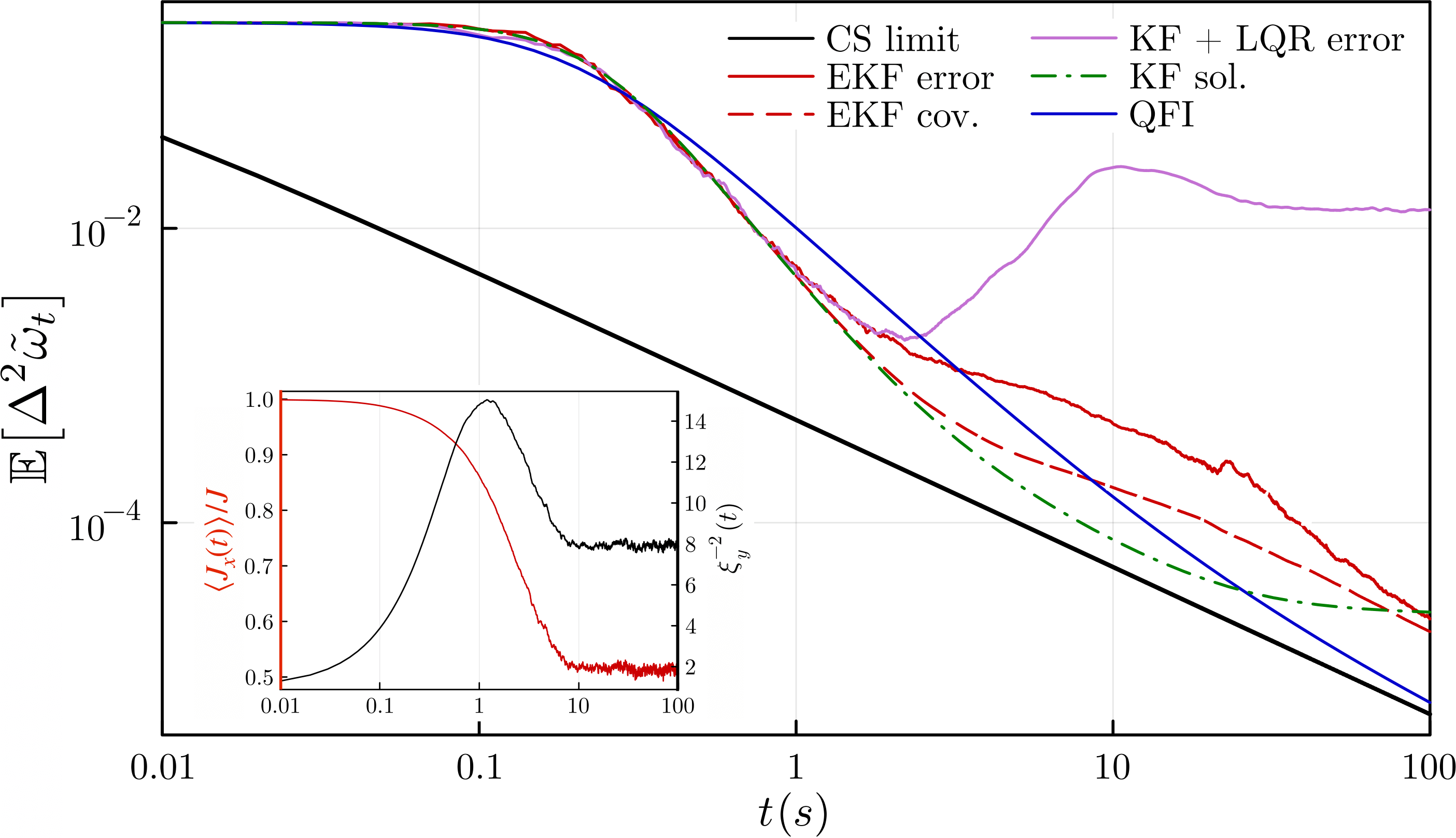
Figure 6: Benchmarking against the classical strategy with weak collective decoherence (${\kappa_{\mathrm{coll}}\ll M}$, ${\kappa_{\mathrm{loc}}=0}$). The evolution of the aMSE in estimating $\omega$ for various estimation+control schemes is plotted against the QCRB (103) applicable to classical strategies with a strong measurement (solid blue). The covariances provided by the estimators (EKF in dashed red and KF in dash-dotted green) correctly predict the true error only within the LG regime (${t\lesssim(M+\kappa_{\mathrm{coll}})^{-1}\!\!\approx\!3\mathrm{s}}$), while the CS limit (10) (solid black) is not attained. The inset depicts the evolution of the spin-squeezing parameter (8) (black) and the ensemble polarisation (red) for the EKF+LQR scheme, for which the atoms maintain spin-squeezing. Parameters chosen: $N=100$, $\kappa_{\mathrm{coll}}=0.0005$, $M=0.3$, $\omega=1$ and $\eta=1$. The data is averaged over $\nu=1000$ trajectories and the EKF is initialised as in Fig. 3.

E.0.3 Collective decoherence

In the case of collective decoherence, we resort to computing the QFI (104) numerically, what we demonstrate to be possible efficiently in the angular momentum basis. In particular, by rewriting the initial CCS state in the $\{\hat{J}^{2},\hat{J}_{z}\}$-basis, i.e. $\ket{\mathrm{CSS}_{x}}=\sum_{m=-J}^{J}b_{J,m}\ket{J,m}$ with $b_{J,k}=\frac{1}{2^{J}}\binom{2J}{J+k}^{1/2}$ and $J=N/2$, we obtain the expression for the state of atomic ensemble at time $t$ as

$$\rho_{t}=\Lambda_{\mathrm{coll}}\!\left[\ket{\mathrm{CSS}_{x}}\!\bra{\mathrm{CSS}_{x}}\right]=$$

$$=\!\!\!\!\!\sum_{n,m=-J}^{J}\!\!\!b_{J,n}b_{J,m}\,\mathrm{e}^{-\kappa_{\mathrm{coll}}\,t\,(m-n)^{2}/2}|J,n\rangle\langle J,m|,$$ (108)

whose dimension scales linearly with $N$. Hence, we can perform numerically its eigendecomposition, $\rho_{t}|k\rangle=\lambda_{k}|k\rangle$, for all $N\lesssim 300$ of relevance. As a result, we may compute the QFI using the expression [88, 89]:

$$\mathcal{F}[\rho_{t},\hat{J}_{z}]=2t^{2}\,\sum_{k,l}\frac{(\lambda_{k}-\lambda_{l})^{2}}{(\lambda_{k}+\lambda_{l})}|\langle k|\hat{J}_{z}|l\rangle|^{2},$$ (109)

with every eigenvector $\ket{k}$ known in the angular momentum basis $\ket{J,m}$, and $\hat{J}_{z}=\sum_{m=-J}^{J}m\ket{J,m}\!\bra{J,m}$. Substituting the QFI (109) into the QBCRB (103), we obtain an expression similar to Eq. (107), which we evaluate numerically to obtain a universal lower bound on the aMSE for the classical strategy with collective decoherence.

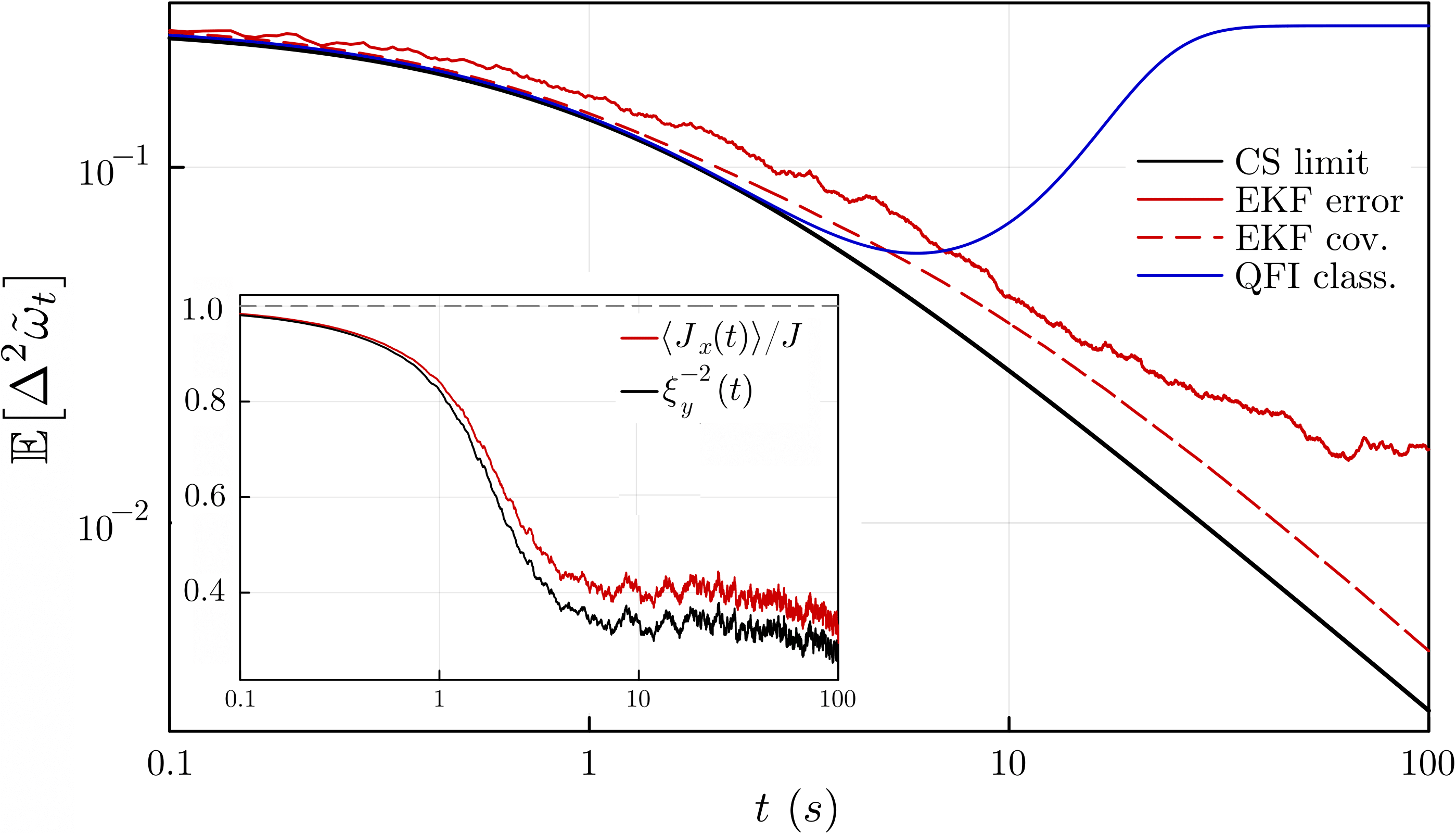
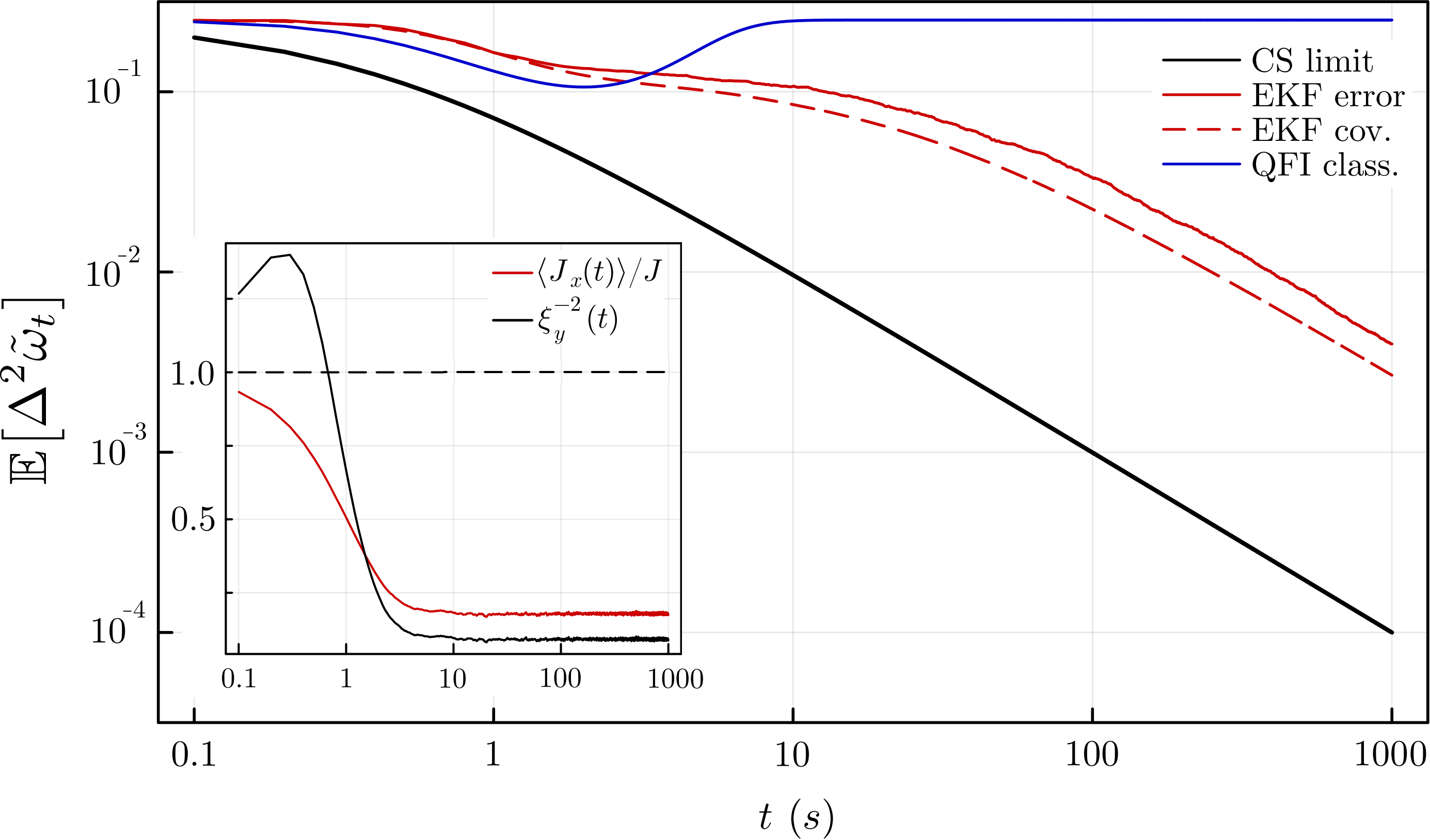
Figure 7: Benchmarking against the classical strategy with strong decoherence. The aMSE attained by the EKF+LQR scheme (red) is shown as a function of time against the QCRB (103) applicable to classical strategies with a strong measurement (blue) for: (a)–collective decoherence (${\kappa_{\mathrm{coll}}\approx M}$, ${\kappa_{\mathrm{loc}}=0}$); and (b)–local decoherence (${\kappa_{\mathrm{loc}}\approx M}$, ${\kappa_{\mathrm{coll}}=0}$). Covariances of the EKF are marked in dashed red along with the CS limit (10) (black). The insets depict evolution of the spin-squeezing parameter (8) (black) and the ensemble polarisation (red), but observing spin-squeezing ($\mathbb{E}\!\left[{\xi^{-2}_{y}}\right]>1$) is impossible for $\kappa_{\mathrm{coll}}\geq M$ [35]. $N=100$ and $\kappa_{\mathrm{coll}}=M=0.3$ in (a), whereas $N=10$ and $\kappa_{\mathrm{loc}}=M=0.5$ in (b) ($\omega=1$, $\eta=1$ in both). The aMSEs are averaged over $\nu=1000$ trajectories and the EKF is initialised as in Fig. 3.

E.0.4 Benchmarking the estimation+control schemes

In Fig. 6, we consider weak collective decoherence ($\kappa_{\mathrm{loc}}=0$, $\kappa_{\mathrm{coll}}\ll M$) and compare the aMSEs attained by different schemes involving continuous probing against the QBCRB (103) applicable for the classical strategy (blue). As expected, out of all estimation+control schemes the EKF+LQR strategy (red solid) yields best results, and clearly surpasses the limit imposed on classical strategies. However, this occurs as short timescales within the LG regime, $t\lesssim(M+\kappa_{\mathrm{coll}})^{-1}$, at which KF (pink) could also be used, instead despite quickly becoming unreliable at longer times. Moreover, due to low atomic number, $N=100$, the covariance $\sigma_{\omega\omega}$ of the EKF (dashed red) and KF (dot-dashed green, derived by us in Ref. [35]) correctly predict the true errors only at very short times at which the CoG model (4) can be trusted. Although the QCRB (103) in Fig. 6 indicates that at longer times the classical strategy involving a strong measurement may attain lower aMSEs, this is only a consequence of choosing decoherence very weak and, hence, very long coherence time, $\kappa_{\mathrm{coll}}^{-1}\approx 10^{4}$ s, beyond which the strong measurement provides no information about $\omega$.

In order to emphasise this behaviour and see the clear benefits of using the EKF+LQR scheme, we significantly increase the strength of decoherence, either collective or local in Fig. 7(a) or (b), respectively, so that it is comparable with the strength of the QND-measurement used for continuous probing. From Fig. 7, it is clear that in both cases, while the EKF+LQR schemes keeps the atomic state polarised (see red lines within the insets) and, hence, the aMSE decreasing, the classical strategy becomes useless beyond the coherence time ($1/\kappa_{\mathrm{coll}}$ or $1/\kappa_{\mathrm{loc}}$) of the atomic ensemble.

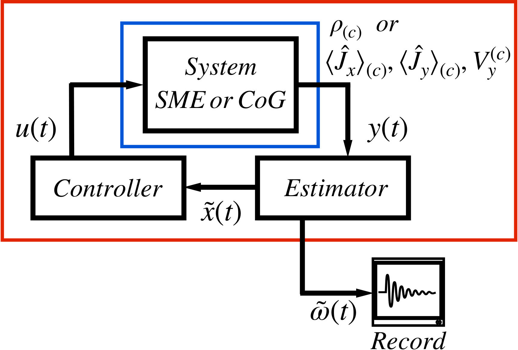
Figure 8: Information flow within the setup of Fig. 1. Basic building blocks: system, estimator and controller, all connected in a closed feedback loop. The outputs of the system can either be the conditional state $\rho_{\scriptscriptstyle\mathrm{(c)}}(t)$ or the state-vector $\boldsymbol{x}(t)$ containing first and second moments (e.g. $\big{\langle}\hat{J}_{x}\big{\rangle}_{\!\scriptscriptstyle\mathrm{(c)}}$, $\big{\langle}\hat{J}_{y}\big{\rangle}_{\!\scriptscriptstyle\mathrm{(c)}}$, $\mathrm{V}_{y}^{\scriptscriptstyle\mathrm{(c)}}$), depending on how we simulate the system, either with SME (2) or CoG (4), respectively. From the system output we construct the photocurrent $y(t)$ according to Eq. (1), which is fed into a filter that produces real-time estimates $\tilde{\boldsymbol{x}}(t)$, which are then used by a controller to devise a control signal $u(t)$ to steer the state of the system. Assessing the fidelity of the CoG approximation in replicating the evolution of the system can be performed at two different stages: by analysing the system dynamics itself (output of the blue box) or focussing only on the $\omega$-estimation task (output of the red box).

Appendix F Verification of the CoG approximation

Fig. 8 presents the architecture of the feedback loop exploited within our atomic magnetometry scheme. The detection data $\boldsymbol{y}(t)$ in each round is generated by simulating the ‘System’ either exactly – its full conditional density matrix $\rho_{\scriptscriptstyle\mathrm{(c)}}$ with help of the SME (2); or approximately – tracking only the dynamics of its relevant first and second moments, $\big{\langle}\hat{J}_{x}\big{\rangle}_{\!\scriptscriptstyle\mathrm{(c)}}$, $\big{\langle}\hat{J}_{y}\big{\rangle}_{\!\scriptscriptstyle\mathrm{(c)}}$ and $\mathrm{V}_{y}^{\scriptscriptstyle\mathrm{(c)}}$, assuming them to be governed by the CoG model (4).

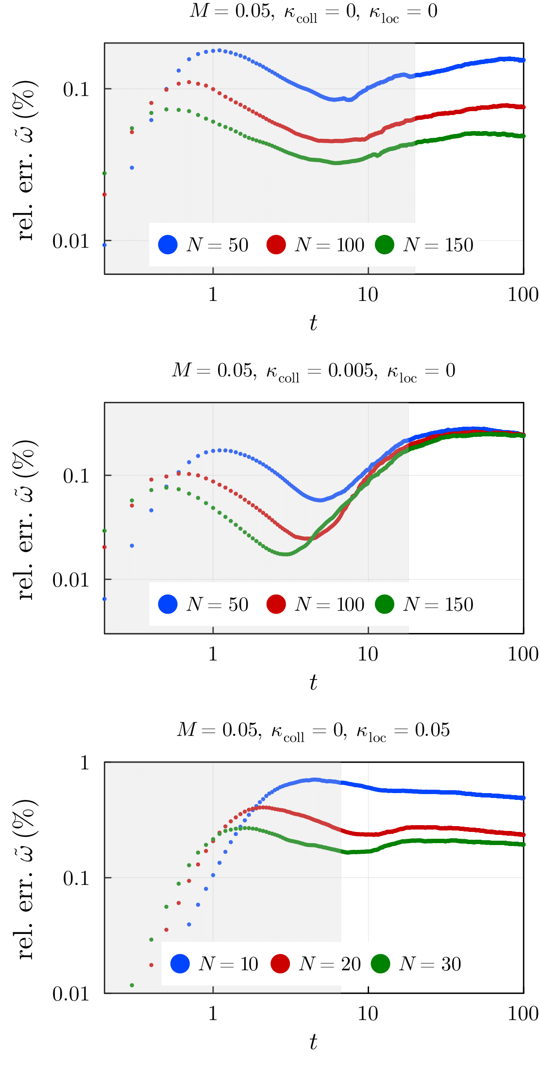
Figure 9: Evolution of the relative error in estimating the Larmor frequency when comparing the exact (SME (2)) and the approximate (COG (4)) models. Each graph shows the relative error in percentage for three different noisy scenarios (top to bottom): with the decoherence induced solely by the continuous measurement, with both measurement-induced and collective decoherence, with all measurement-induced, collective and local decoherence. In each plot, various system sizes are considered: $N=50,100,150$ (blue, red and green, respectively) for the first two cases and $N=10,20,30$ (also blue, red and green, respectively) in presence of also the local decoherence. Each plot demonstrates that the CoG approximation can be used to simulate the dynamics of the system and still get accurate estimations of the Larmor frequency compared when using the exact model (errors always below 1%). Additionally, all plots show a decrease in the relative error when increasing the system size within the LG regime (shaded pink area), and for the case of only measurement decoherence and local decoherence, also outside of it. All errors above are obtained upon averaging over $\nu=1000$ measurement trajectories.

The so-simulated measurement record is interpreted by the ‘Estimator’ (i.e. the EKF) providing in real time not only the estimate of the Larmor frequency $\tilde{\omega}(t)$, but also dynamical parameters $\tilde{\boldsymbol{x}}(t)$ that are in turn used by the ‘Controller’ (i.e. the LQR) to modify “on the fly” the system dynamics being simulated by changing $u(t)$.

To assess the accuracy of the CoG approximation (4) in simulating the system dynamics—in contrast to the estimator construction, in which case the EKF is always built based on the CoG model—we benchmark it against the exact SME (2) solution for moderate atomic number, for which the latter can still be efficiently performed. In what follows, we perform the comparison at two levels. Firstly, we focus only on the estimation task and, in particular, compute the average discrepancy only when requiring the scheme to accurately provide (on average) $\tilde{\omega}(t)$ in real time (red box in Fig. 8). Secondly, we are more restrictive and require further the relevant moments, $\big{\langle}\hat{J}_{x}\big{\rangle}_{\!\scriptscriptstyle\mathrm{(c)}}$, $\big{\langle}\hat{J}_{y}\big{\rangle}_{\!\scriptscriptstyle\mathrm{(c)}}$ and $\mathrm{V}_{y}^{\scriptscriptstyle\mathrm{(c)}}$, to be accurately reproduced by comparing their average error when compared to their exact values computed with help of $\rho_{\scriptscriptstyle\mathrm{(c)}}$ (blue box in Fig. 8)—so that they may be directly used, e.g. to estimate the spin-squeezing as in Fig. 4.

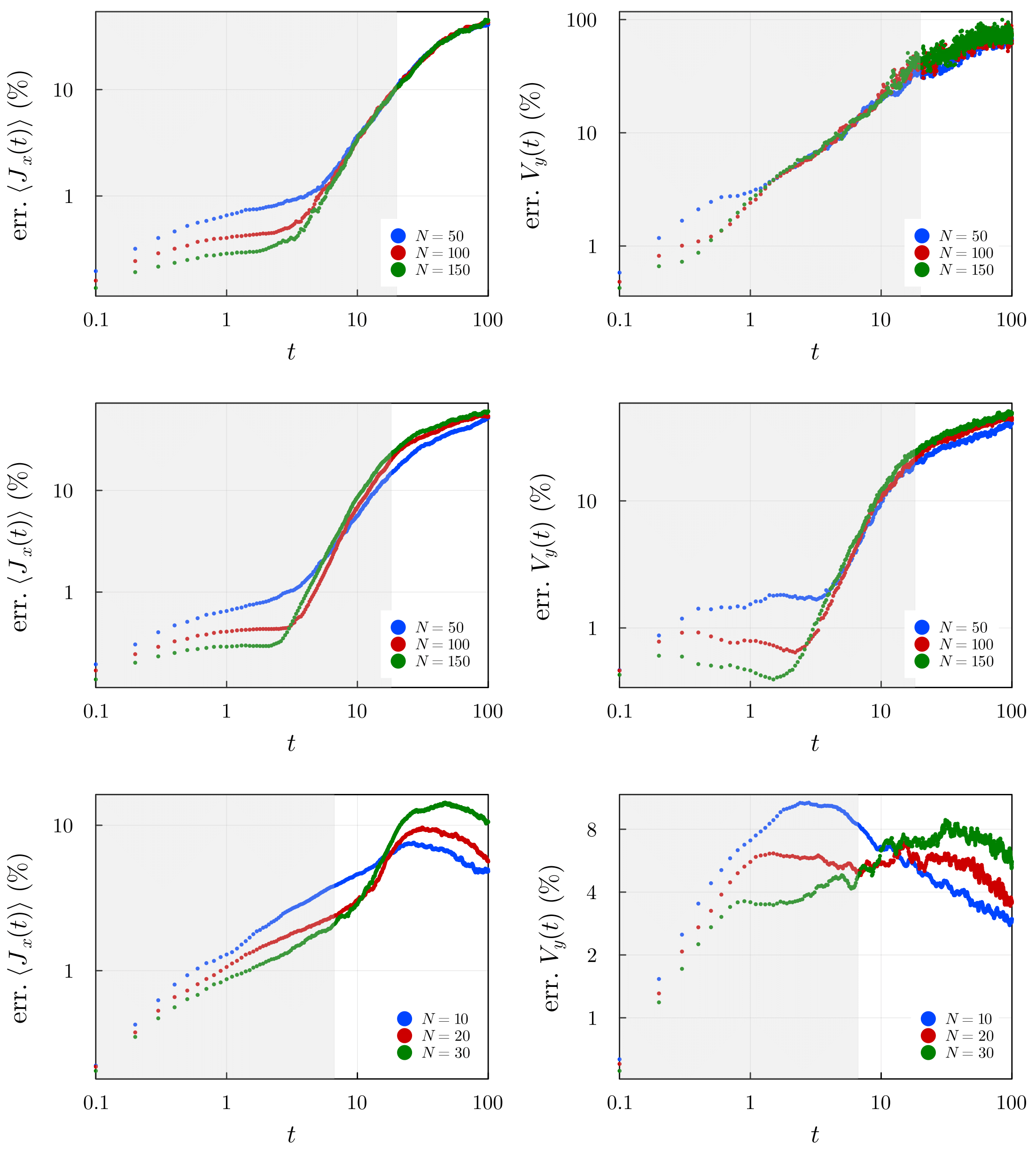
Figure 10: Comparative error analysis of moments $\langle\hat{J}_{x}\rangle$ and $\mathrm{V}_{y}$ between the exact and the CoG model. Each plot presents the relative error (in %) in simulating the first and second moments, $\mathrm{x}\in\{\langle\hat{J}_{x}\rangle,\mathrm{V}_{y}\}$, with the approximate CoG model (4) as compared to solving the exact SME (2). The formula for the presented error, $\mathbb{E}\!\left[{\delta_{\mathrm{x}}}\right]$, can be found in the text below. The comparative analysis is done for three different types of decoherence: top row – induced by the continuous measurement ($M=0.05$, $\kappa_{\mathrm{coll}}=\kappa_{\mathrm{loc}}=0$), middle row – measurement-induced and collective ($M=0.05$, $\kappa_{\mathrm{coll}}=0.005$, $\kappa_{\mathrm{loc}}=0$), bottom row – measurement-induced and local ($M=0.05$, $\kappa_{\mathrm{coll}}=0$, $\kappa_{\mathrm{loc}}=0.05$). In each graph we plot the error for systems of increasing size (either $N=50,100,150$ or $N=10,20,30$ for local noise) to show how for short times we expect the CoG approximation to become more accurate as $N$ increases. All errors above are obtained upon averaging over $\nu=1000$ measurement trajectories.

In Fig. 9, we present in percentage the average relative error (ARE) between the real-time estimate $\tilde{\omega}(t)$ of $\omega$ obtained using the exact model (full SME solution) and the approximate model (CoG), i.e. $\mathbb{E}\!\left[{\delta_{\tilde{\omega}}}\right]\coloneqq 100\%\times\mathbb{E}\!\left[{|(\tilde{\omega}_{SME}-\tilde{\omega}_{CoG})/\tilde{\omega}_{SME}|}\right]=100\%\times\int\!d\omega\,p(\omega)\int\!\mathcal{D}\boldsymbol{y}_{\leq t}\,p(\boldsymbol{y}_{\leq t}|\omega)|(\tilde{\omega}_{SME}-\tilde{\omega}_{CoG})/\tilde{\omega}_{SME}|$. Fig. 9 showcases three plots, each corresponding to a different noise scenario: measurement decoherence, combined measurement and collective decoherence, and combined measurement and local decoherence, arranged from top to bottom. Each plot shows the averaged relative error for increasing system sizes — specifically, $N=50,100,150$ for the first two scenarios, and $N=10,20,30$ for the local case. The plots demonstrate that as the system size increases, the Larmor frequency estimate derived using the CoG approximation either aligns more closely with the estimate given by solving the SME exactly, or maintains an error margin below 1%. This trend leads us to conclude that for large ensembles with $N\sim 10^{5}-10^{14}$, the CoG approximation proves to be sufficiently accurate to generate the measurement data needed to estimate the Larmor frequency.

However, to evaluate the reliability of the CoG approximation (4) itself, we verify its ability to reproduce the key system dynamical properties, in particular, the moments necessary to compute the spin-squeezing parameter (8), $\big{\langle}\hat{J}_{x}\big{\rangle}_{\!\scriptscriptstyle\mathrm{(c)}}$ and $\mathrm{V}_{y}^{\scriptscriptstyle\mathrm{(c)}}$, as compared with their true values obtained from $\rho_{\scriptscriptstyle\mathrm{(c)}}$ provided by the exact solution of the SME (2) (compare the outputs of the blue box in Fig. 8). For a quantitative assessment, as detailed in Fig. 10, we employ the error metric $\mathbb{E}\!\left[{\delta_{\mathrm{x}}}\right]=100\times\mathbb{E}\!\left[{|\mathrm{x}_{\mathrm{SME}}-\mathrm{x}_{\mathrm{CoG}}|}\right]/\mathbb{E}\!\left[{|\mathrm{x}_{\mathrm{SME}}|}\right]$, where $\mathrm{x}$ in our case can be either $\big{\langle}\hat{J}_{x}\big{\rangle}_{\!\scriptscriptstyle\mathrm{(c)}}$ or $\mathrm{V}_{y}^{\scriptscriptstyle\mathrm{(c)}}$. In Fig. 10, each subplot illustrates that, for short times, the simulation error decreases as the system size increases. However, as time progresses, this trend is halted with the error in simulating first and second moments escalating significantly. Nonetheless, for times shorter than $t\lesssim 1/(M+\kappa_{\mathrm{coll}}+2\kappa_{\mathrm{loc}})$ , the CoG simulation error for these moments is kept below $\sim$ 10%. This finding supports the use of the CoG approximation to accurately predict the squeezing parameter of large atomic ensembles, e.g. with $N$ as big as $10^{5}-10^{14}$, at short times below $t\lesssim 1/(M+\kappa_{\mathrm{coll}}+2\kappa_{\mathrm{loc}})$.

References

- Budker and Romalis [2007] D. Budker and M. Romalis, “Optical magnetometry,” Nat. Phys. 3, 227 (2007).
- Clarke and Braginski [2004] J. Clarke and A. I. Braginski, The Squid Handbook, Vol. 1 (Wiley Online Library, 2004).
- Kitching [2018] J. Kitching, “Chip-scale atomic devices,” Appl. Phys. Rev. 5, 031302 (2018).
- Jensen et al. [2018] K. Jensen, M. A. Skarsfeldt, H. Stærkind, J. Arnbak, M. V. Balabas, S.-P. Olesen, B. H. Bentzen, and E. S. Polzik, “Magnetocardiography on an isolated animal heart with a room-temperature optically pumped magnetometer,” Sci. Rep. 8, 16218 (2018).
- Boto et al. [2018] E. Boto, N. Holmes, J. Leggett, G. Roberts, V. Shah, S. S. Meyer, L. D. Muñoz, K. J. Mullinger, T. M. Tierney, S. Bestmann, G. R. Barnes, R. Bowtell, and M. J. Brookes, “Moving magnetoencephalography towards real-world applications with a wearable system,” Nature 555, 657 (2018).
- Limes et al. [2020] M. E. Limes, E. L. Foley, T. W. Kornack, S. Caliga, S. McBride, A. Braun, W. Lee, V. G. Lucivero, and M. V. Romalis, “Portable Magnetometry for Detection of Biomagnetism in Ambient Environments,” Phys. Rev. Applied 14, 011002 (2020).
- Zhang et al. [2020] R. Zhang, W. Xiao, Y. Ding, Y. Feng, X. Peng, L. Shen, C. Sun, T. Wu, Y. Wu, Y. Yang, Z. Zheng, X. Zhang, J. Chen, and H. Guo, “Recording brain activities in unshielded Earth’s field with optically pumped atomic magnetometers,” Sci. Adv. 6, eaba8792 (2020).
- Pospelov et al. [2013] M. Pospelov, S. Pustelny, M. P. Ledbetter, D. F. J. Kimball, W. Gawlik, and D. Budker, “Detecting domain walls of axionlike models using terrestrial experiments,” Phys. Rev. Lett. 110, 021803 (2013).
- Pustelny et al. [2013] S. Pustelny, D. F. J. Kimball, C. Pankow, M. P. Ledbetter, P. Wlodarczyk, P. Wcislo, M. Pospelov, J. R. Smith, J. Read, W. Gawlik, and D. Budker, “The Global Network of Optical Magnetometers for Exotic physics (GNOME): A novel scheme to search for physics beyond the Standard Model,” Ann. Phys. 525, 659 (2013).
- Kuzmich et al. [2000] A. Kuzmich, L. Mandel, and N. P. Bigelow, “Generation of spin squeezing via continuous quantum nondemolition measurement,” Phys. Rev. Lett. 85, 1594 (2000).
- Shah et al. [2010] V. Shah, G. Vasilakis, and M. V. Romalis, “High bandwidth atomic magnetometery with continuous quantum nondemolition measurements,” Phys. Rev. Lett. 104, 013601 (2010).
- Kong et al. [2020] J. Kong, R. Jiménez-Martínez, C. Troullinou, V. G. Lucivero, G. Tóth, and M. W. Mitchell, “Measurement-induced, spatially-extended entanglement in a hot, strongly-interacting atomic system,” Nat. Commun. 11, 2415 (2020).
- Kuzmich et al. [1998] A. Kuzmich, N. P. Bigelow, and L. Mandel, “Atomic quantum non-demolition measurements and squeezing,” Europhys. Lett. 42, 481 (1998).
- Sewell et al. [2012] R. J. Sewell, M. Koschorreck, M. Napolitano, B. Dubost, N. Behbood, and M. W. Mitchell, “Magnetic sensitivity beyond the projection noise limit by spin squeezing,” Phys. Rev. Lett. 109, 253605 (2012).
- Koschorreck et al. [2010] M. Koschorreck, M. Napolitano, B. Dubost, and M. W. Mitchell, “Sub-projection-noise sensitivity in broadband atomic magnetometry,” Phys. Rev. Lett. 104, 093602 (2010).
- Wasilewski et al. [2010] W. Wasilewski, K. Jensen, H. Krauter, J. J. Renema, M. V. Balabas, and E. S. Polzik, “Quantum noise limited and entanglement-assisted magnetometry,” Phys. Rev. Lett. 104, 133601 (2010).
- Aspelmeyer et al. [2014] M. Aspelmeyer, T. J. Kippenberg, and F. Marquardt, “Cavity optomechanics,” Rev. Mod. Phys. 86, 1391 (2014).
- Iwasawa et al. [2013] K. Iwasawa, K. Makino, H. Yonezawa, M. Tsang, A. Davidovic, E. Huntington, and A. Furusawa, “Quantum-limited mirror-motion estimation,” Phys. Rev. Lett. 111, 163602 (2013).
- Wieczorek et al. [2015] W. Wieczorek, S. G. Hofer, J. Hoelscher-Obermaier, R. Riedinger, K. Hammerer, and M. Aspelmeyer, “Optimal State Estimation for Cavity Optomechanical Systems,” Phys. Rev. Lett. 114, 223601 (2015).
- Rossi et al. [2019] M. Rossi, D. Mason, J. Chen, and A. Schliesser, “Observing and Verifying the Quantum Trajectory of a Mechanical Resonator,” Phys. Rev. Lett. 123, 163601 (2019).
- Wilson et al. [2015] D. J. Wilson, V. Sudhir, N. Piro, R. Schilling, A. Ghadimi, and T. J. Kippenberg, “Measurement-based control of a mechanical oscillator at its thermal decoherence rate,” Nature 524, 325 (2015).
- Rossi et al. [2018] M. Rossi, D. Mason, J. Chen, Y. Tsaturyan, and A. Schliesser, “Measurement-based quantum control of mechanical motion,” Nature 563, 53 (2018).
- Sudhir et al. [2017] V. Sudhir, D. J. Wilson, R. Schilling, H. Schütz, S. A. Fedorov, A. H. Ghadimi, A. Nunnenkamp, and T. J. Kippenberg, “Appearance and disappearance of quantum correlations in measurement-based feedback control of a mechanical oscillator,” Phys. Rev. X 7, 011001 (2017).
- Setter et al. [2018] A. Setter, M. Toroš, J. F. Ralph, and H. Ulbricht, “Real-time kalman filter: Cooling of an optically levitated nanoparticle,” Phys. Rev. A 97, 033822 (2018).
- Magrini et al. [2021] L. Magrini, P. Rosenzweig, C. Bach, A. Deutschmann-Olek, S. G. Hofer, S. Hong, N. Kiesel, A. Kugi, and M. Aspelmeyer, “Real-time optimal quantum control of mechanical motion at room temperature,” Nature 595, 373 (2021).
- Ernzer et al. [2023] M. Ernzer, M. Bosch Aguilera, M. Brunelli, G.-L. Schmid, T. M. Karg, C. Bruder, P. P. Potts, and P. Treutlein, “Optical coherent feedback control of a mechanical oscillator,” Phys. Rev. X 13, 021023 (2023).
- Nurdin and Yamamoto [2017] H. I. Nurdin and N. Yamamoto, Linear Dynamical Quantum Systems (Springer, 2017).
- Hamerly and Mabuchi [2012] R. Hamerly and H. Mabuchi, “Advantages of coherent feedback for cooling quantum oscillators,” Phys. Rev. Lett. 109, 173602 (2012).
- Yamamoto [2014] N. Yamamoto, “Coherent versus measurement feedback: Linear systems theory for quantum information,” Phys. Rev. X 4, 041029 (2014).
- Geremia et al. [2003] J. M. Geremia, J. K. Stockton, A. C. Doherty, and H. Mabuchi, “Quantum Kalman filtering and the Heisenberg limit in atomic magnetometry,” Phys. Rev. Lett. 91, 250801 (2003).
- Stockton et al. [2004] J. K. Stockton, J. M. Geremia, A. C. Doherty, and H. Mabuchi, “Robust quantum parameter estimation: Coherent magnetometry with feedback,” Phys. Rev. A 69, 032109 (2004).
- Deutsch and Jessen [2010] I. H. Deutsch and P. S. Jessen, “Quantum control and measurement of atomic spins in polarization spectroscopy,” Opt. Commun. 283, 681 (2010).
- Rossi et al. [2021] M. A. C. Rossi, F. Albarelli, D. Tamascelli, and M. G. Genoni, “Qcontinuousmeasurement.jl (2021),” https://github.com/matteoacrossi/QContinuousMeasurement.jl (2021).
- Ma et al. [2011] J. Ma, X. Wang, C. P. Sun, and F. Nori, “Quantum spin squeezing,” Phys. Rep. 509, 89 (2011).
- Amorós-Binefa and Kołodyński [2021] J. Amorós-Binefa and J. Kołodyński, “Noisy atomic magnetometry in real time,” New J. Phys. 23, 123030 (2021).
- Rossi et al. [2020] M. A. C. Rossi, F. Albarelli, D. Tamascelli, and M. G. Genoni, “Noisy Quantum Metrology Enhanced by Continuous Nondemolition Measurement,” Phys. Rev. Lett. 125, 200505 (2020).
- Crassidis and Junkins [2011] J. L. Crassidis and J. L. Junkins, Optimal Estimation of Dynamic Systems, Chapman & Hall/CRC Applied Mathematics & Nonlinear Science (CRC Press, 2011).
- Simon [2006] D. Simon, Optimal State Estimation: Kalman, H Infinity, and Nonlinear Approaches (Wiley, 2006).
- Muñoz Arias et al. [2020] M. H. Muñoz Arias, P. M. Poggi, P. S. Jessen, and I. H. Deutsch, “Simulating nonlinear dynamics of collective spins via quantum measurement and feedback,” Phys. Rev. Lett. 124, 110503 (2020).
- Pezzè et al. [2018] L. Pezzè, A. Smerzi, M. K. Oberthaler, R. Schmied, and P. Treutlein, “Quantum metrology with nonclassical states of atomic ensembles,” Rev. Mod. Phys. 90, 035005 (2018).
- [41] J. Amorós-Binefa and J. Kołodyński, in preparation.
- Budker and Jackson Kimball [2013] D. Budker and D. F. Jackson Kimball, eds., Optical Magnetometry (Cambridge University Press, 2013).
- Geremia et al. [2006] J. M. Geremia, J. K. Stockton, and H. Mabuchi, “Tensor polarizability and dispersive quantum measurement of multilevel atoms,” Phys. Rev. A 73, 042112 (2006).
- Belavkin [1989] V. P. Belavkin, in Modeling and Control of Systems, edited by A. Blaquiére (Springer Berlin Heidelberg, Berlin, Heidelberg, 1989) pp. 245–265.
- van Handel et al. [2005] R. van Handel, J. K. Stockton, and H. Mabuchi, “Modelling and feedback control design for quantum state preparation,” J. Opt. B: Quantum Semiclass. Opt. 7, S179 (2005).
- Gardiner et al. [1985] C. W. Gardiner et al., Handbook of Stochastic Methods, Vol. 3 (Springer Berlin, 1985).
- Chase and Geremia [2008] B. A. Chase and J. M. Geremia, “Collective processes of an ensemble of spin-1/2 particles,” Phys. Rev. A 78, 052101 (2008).
- Baragiola et al. [2010] B. Q. Baragiola, B. A. Chase, and J. Geremia, “Collective uncertainty in partially polarized and partially decohered spin- systems,” Phys. Rev. A 81, 032104 (2010).
- Shammah et al. [2018] N. Shammah, S. Ahmed, N. Lambert, S. De Liberato, and F. Nori, “Open quantum systems with local and collective incoherent processes: Efficient numerical simulations using permutational invariance,” Phys. Rev. A 98, 063815 (2018).
- Rouchon and Ralph [2015] P. Rouchon and J. F. Ralph, “Efficient quantum filtering for quantum feedback control,” Phys. Rev. A 91, 012118 (2015).
- Albarelli et al. [2018] F. Albarelli, M. A. C. Rossi, D. Tamascelli, and M. G. Genoni, “Restoring heisenberg scaling in noisy quantum metrology by monitoring the environment,” Quantum 2, 110 (2018).
- Albarelli et al. [2017] F. Albarelli, M. A. C. Rossi, M. G. A. Paris, and M. G. Genoni, “Ultimate limits for quantum magnetometry via time-continuous measurements,” New J. Phys. 19, 123011 (2017).
- Madsen and Mølmer [2004] L. B. Madsen and K. Mølmer, “Spin squeezing and precision probing with light and samples of atoms in the gaussian description,” Phys. Rev. A 70, 052324 (2004).
- Mølmer and Madsen [2004] K. Mølmer and L. B. Madsen, “Estimation of a classical parameter with gaussian probes: Magnetometry with collective atomic spins,” Phys. Rev. A 70, 052102 (2004).
- Van Trees and Bell [2007] H. L. Van Trees and K. L. Bell, Bayesian Bounds for Parameter Estimation and Nonlinear Filtering/Tracking (Wiley-IEEE Press, 2007).
- Kalman [1960] R. E. Kalman, “A New Approach to Linear Filtering and Prediction Problems,” J Basic Eng-t Asme 82, 35 (1960).
- Kalman and Bucy [1961] R. E. Kalman and R. S. Bucy, “New Results in Linear Filtering and Prediction Theory,” J Basic Eng-t Asme 83, 95 (1961).
- Julier et al. [1995] S. J. Julier, J. K. Uhlmann, and H. F. Durrant-Whyte, in Proceedings of 1995 American Control Conference - ACC’95, Vol. 3 (1995) pp. 1628–1632 vol.3.
- Julier et al. [2000] S. Julier, J. Uhlmann, and H. F. Durrant-Whyte, “A new method for the nonlinear transformation of means and covariances in filters and estimators,” IEEE Trans. Autom. Control 45, 477 (2000).
- Kurdziałek et al. [2023] S. Kurdziałek, W. Górecki, F. Albarelli, and R. Demkowicz-Dobrzański, “Using adaptiveness and causal superpositions against noise in quantum metrology,” Phys. Rev. Lett. 131, 090801 (2023).
- Caprotti et al. [2023] A. Caprotti, M. Barbiero, M. Tarallo, M. Genoni, and G. Bertaina, “Analysis of spin-squeezing generation in cavity-coupled atomic ensembles with continuous measurements,” arXiv:2311.15725 (2023).
- Kitagawa and Ueda [1993] M. Kitagawa and M. Ueda, “Squeezed spin states,” Phys. Rev. A 47, 5138 (1993).
- Wineland et al. [1994] D. J. Wineland, J. J. Bollinger, W. M. Itano, and D. J. Heinzen, “Squeezed atomic states and projection noise in spectroscopy,” Phys. Rev. A 50, 67 (1994).
- Bohnet et al. [2014] J. G. Bohnet, K. C. Cox, M. A. Norcia, J. M. Weiner, Z. Chen, and J. K. Thompson, “Reduced spin measurement back-action for a phase sensitivity ten times beyond the standard quantum limit,” Nat. Photonics 8, 731 (2014).
- Hosten et al. [2016] O. Hosten, N. J. Engelsen, R. Krishnakumar, and M. A. Kasevich, “Measurement noise 100 times lower than the quantum-projection limit using entangled atoms,” Nature 529, 505 (2016).
- Bao et al. [2020] H. Bao, J. Duan, S. Jin, X. Lu, P. Li, W. Qu, M. Wang, I. Novikova, E. E. Mikhailov, K.-F. Zhao, K. Mølmer, H. Shen, and Y. Xiao, “Spin squeezing of atoms by prediction and retrodiction measurements,” Nature 581, 159 (2020).
- Fritsche et al. [2014] C. Fritsche, E. Özkan, L. Svensson, and F. Gustafsson, in 17th International Conference on Information Fusion (FUSION) (IEEE, Salamanca, Spain, 2014) pp. 1–8.
- Matsumoto [2010] K. Matsumoto, “On metric of quantum channel spaces,” (2010), arxiv:1006.0300 [quant-ph] .
- Demkowicz-Dobrzański et al. [2012] R. Demkowicz-Dobrzański, J. Kołodyński, and M. Guţă, “The elusive Heisenberg limit in quantum-enhanced metrology,” Nat. Commun. 3, 1063 (2012).
- Wiseman [1994] H. M. Wiseman, “Quantum theory of continuous feedback,” Phys. Rev. A 49, 2133 (1994).
- Thomsen et al. [2002] L. K. Thomsen, S. Mancini, and H. M. Wiseman, “Spin squeezing via quantum feedback,” Phys. Rev. A 65, 061801 (2002).
- Note [1] Within our observation model (12), the function is linear, so that is time-invariant.
- Note [2] For polarisation, despite , the unconditional dynamics of cannot be simply determined from Eq. (2) due to the presence of the control .
- Note [3] Choosing, e.g., would yield zero error at and naively suggest the CS limit (10) to be then “breached”, what cannot happen when explicitly averaging over .
- Carleo et al. [2019] G. Carleo, I. Cirac, K. Cranmer, L. Daudet, M. Schuld, N. Tishby, L. Vogt-Maranto, and L. Zdeborová, “Machine learning and the physical sciences,” Rev. Mod. Phys. 91, 045002 (2019).
- Dawid et al. [2023] A. Dawid, J. Arnold, B. Requena, A. Gresch, M. Płodzień, K. Donatella, K. A. Nicoli, P. Stornati, R. Koch, M. Büttner, R. Okuła, G. Muñoz-Gil, R. A. Vargas-Hernández, A. Cervera-Lierta, J. Carrasquilla, V. Dunjko, M. Gabrié, P. Huembeli, E. van Nieuwenburg, F. Vicentini, L. Wang, S. J. Wetzel, G. Carleo, E. Greplová, R. Krems, F. Marquardt, M. Tomza, M. Lewenstein, and A. Dauphin, “Modern applications of machine learning in quantum sciences,” arXiv:2204.04198 10.48550/arXiv.2204.04198 (2023).
- Note [4] However, in case of KF and (quantum) LG dynamics, its covariance does not depend on a particular measurement trajectory and, hence, can be computed without inspecting it.
- Tsang et al. [2009] M. Tsang, J. H. Shapiro, and S. Lloyd, “Quantum theory of optical temporal phase and instantaneous frequency. ii. continuous-time limit and state-variable approach to phase-locked loop design,” Phys. Rev. A 79, 053843 (2009).
- Zhang and Mølmer [2017] J. Zhang and K. Mølmer, “Prediction and retrodiction with continuously monitored gaussian states,” Phys. Rev. A 96, 062131 (2017).
- Helstrom [1976] C. W. Helstrom, Quantum Detection and Estimation Theory (Academic Press, 1976).
- Agarwal [1981] G. S. Agarwal, “Relation between atomic coherent-state representation, state multipoles, and generalized phase-space distributions,” Phys. Rev. A 24, 2889 (1981).
- Schmied and Treutlein [2011] R. Schmied and P. Treutlein, “Tomographic reconstruction of the Wigner function on the Bloch sphere,” New J. Phys. 13, 065019 (2011).
- Bobrovsky et al. [1987] B. Z. Bobrovsky, E. Mayer-Wolf, and M. Zakai, “Some Classes of Global Cramér-Rao Bounds,” Ann. Statist. 15, 1421 (1987).
- Breuer and Petruccione [2002] H.-P. Breuer and F. Petruccione, The Theory of Open Quantum Systems (Oxford University Press, 2002).
- Wiseman and Milburn [2009] H. M. Wiseman and G. J. Milburn, Quantum measurement and control (Cambridge University Press, 2009).
- Albarelli and Genoni [2024] F. Albarelli and M. G. Genoni, “A pedagogical introduction to continuously monitored quantum systems and measurement-based feedback,” Phys. Lett. A 494, 129260 (2024).
- Wiseman and Milburn [1993] H. M. Wiseman and G. J. Milburn, “Quantum theory of field-quadrature measurements,” Phys. Rev. A 47, 642 (1993).
- Tóth and Apellaniz [2014] G. Tóth and I. Apellaniz, “Quantum metrology from a quantum information science perspective,” J. Phys. A: Math. Theor. 47, 424006 (2014).
- Demkowicz-Dobrzański et al. [2015] R. Demkowicz-Dobrzański, M. Jarzyna, and J. Kołodyński, in Progress in Optics, Vol. 60, edited by E. Wolf (Elsevier, 2015) pp. 345–435, arXiv:1405.7703 .