Complete parameterization, and invariance, of diffusive quantum trajectories
for Markovian open systems

Abstract

The state matrix $\rho$ for an open quantum system with Markovian evolution obeys a master equation. The master equation evolution can be unraveled into stochastic nonlinear trajectories for a pure state $P$, such that on average $P$ reproduces $\rho$. Here we give for the first time a complete parameterization of all diffusive unravelings (in which $P$ evolves continuously but non-differentiably in time). We give an explicit measurement theory interpretation for these quantum trajectories, in terms of monitoring the system’s environment. We also introduce new classes of diffusive unravelings that are invariant under the linear operator transformations under which the master equation is invariant. We illustrate these invariant unravelings by numerical simulations. Finally, we discuss generalized gauge transformations as a method of connecting apparently disparate descriptions of the same trajectories by stochastic Schrödinger equations, and their invariance properties.

I Introduction

It is well known that quantum mixtures differ qualitatively from classical mixtures. Here a mixed state means one about which we have incomplete knowledge, as opposed to a pure state, which is one about which we have maximal knowledge. In the classical case, a mixed state is described by a probability distribution $\wp$ over phase space. There is a one-to-one correspondence between this probability distribution $\wp$ and a weighted ensemble of points in phase space (pure states). In the quantum case, a mixed state is described by a density operator, or state matrix $\rho$. But there is a one-to-many (infinitely many, in fact) mapping [3] from this $\rho$ to a weighted ensemble of state vectors (pure states). That is to say, there are infinitely many ways to write a given impure state matrix $\rho$ as a positively weighted sum of projectors.

This difference between quantum and classical systems is also reflected in the dynamics of open systems. Interaction with an environment generically causes systems to become mixed. This can be described by deterministic evolution of the mixed state (the classical $\wp$ or the quantum $\rho$). For example, this evolution may be described by a Fokker-Planck equation for $\wp$, or a master equation for $\rho$. Alternatively, the dynamics can be described by stochastic trajectories of pure states (the classical point in phase space or the quantum projector). In the classical case the two descriptions follow uniquely from each other and they are completely equivalent. But in the quantum case, the trajectory equation does not follow uniquely from the ensemble equation. In fact there are infinitely many different quantum trajectory equations for a given master equation [4, 5].

It is thus apparent that quantum trajectories have a richer physical content than classical trajectories. The different quantum trajectory equations have been called different unravelings of the master equation. In some (but not all [6]) cases, they can be interpreted as arising from inequivalent schemes of efficiently monitoring the environment to which the system is coupled [7]. (For classical systems, all such efficient schemes would be equivalent with one another.) From this point of view, the statistical description arises from the probabilistic nature of quantum measurements. However, it is possible to study the nature of quantum unravelings without specifying a concrete measurement scheme.

In the present work, we limit our discussion to a particular class of unravelings, in which the noise in the quantum trajectory is diffusive in nature. After some preliminaries, we give, for the first time, a complete parameterization of such unravelings in Sec. IV. An explicit formulation in terms of general quantum measurement is given in Sec. V. In Sec. VI we discuss the notion of invariance of quantum trajectories, using concepts from Sec. II. We introduce new classes of invariant unravelings and, in Sec. VII, illustrate them for the process of resonance fluorescence. In Sec. VIII we discuss the stochastic Schrödinger equation formulation of quantum trajectories, and show how seemingly inequivalent equations may be related by generalized gauge transformations. We conclude with a summary and discussion of the relation of our present work to past and future work in the field.

II The Master Equation

If a quantum system is weakly coupled to an environmental reservoir, and many modes of the reservoir are roughly equally affected by the system, then one can make the Born and Markov approximations in describing the effect of the environment on the system [8]. Tracing over (that is, ignoring) the state of the environment leads to a Markovian evolution equation for the state matrix $\rho$ of the system, known as a quantum master equation. The most general form of the quantum master equation which is mathematically valid is the Lindblad form [9]

$$\dot{\rho}={\cal L}\rho\equiv-i[H,\rho]+c_{k}\rho c_{k}^{\dagger}-\mbox{$\frac{1}{2}$}\left\{{c_{k}^{\dagger}c_{k},\rho}\right\}~{}.$$ (1)

Here $\left\{{c_{k}}\right\}_{k=1}^{K}$ is the ordered set of Lindblad operators, and as in the remainder of this paper, we are using the Einstein summation convention for repeated indices. The Lindblad operators couple the system to the reservoir modes.

The above representation of the evolution superoperator ${\cal L}$ is not unique. We can reduce the ambiguity by requiring that the operators $1,c_{1},c_{2},\dots,c_{K}$ be linearly independent. Then we are left with the freedom of re-defining the Lindblad operators by an arbitrary $K\times K$ unitary matrix $T_{kl}$ [10]:

$$c_{k}\rightarrow T_{kl}c_{l}~{}.$$ (2)

Here, as in the remainder of this paper, we are using the Einstein summation convention for repeated indices. In addition, ${\cal L}$ is invariant under c-number shifts of the Lindblad operators, accompanied by a new term in the Hamiltonian

$$c_{k}\rightarrow c_{k}+\chi_{k}~{},~{}~{}~{}~{}H\rightarrow H+\mbox{$\frac{i}{2}$}\left({\chi_{k}^{\star}c_{k}-{\rm H.c.}}\right)~{}.$$ (3)

The master equation turns pure states $\rho=\left|{\psi}\right\rangle\left\langle{\psi}\right|\equiv P$ into mixed ones. A related mathematical object is the transition (mixing) rate operator [11]

$$W = {\cal L}P-\left\{{P,{\cal L}P}\right\}+P{\rm Tr}\left[{P{\cal L}P}\right]$$ (4)

$$= \left({c_{k}-\left\langle{c_{k}}\right\rangle}\right)P\left({c_{k}-\left\langle{c_{k}}\right\rangle}\right)^{\dagger}~{},$$ (5)

where $\left\langle{\dots}\right\rangle={\rm Tr}[\dots P]$ stands for quantum expectation values. $W$ is an invariant operator; it does not change with the unitary rotation (2) of the Lindblad operators or the c-number shift (3). The transition rate operator is positive semi-definite and orthogonal to the current state $P$, i.e. $WP=PW=0$. Its trace is the transition (mixing) rate:

$$w\equiv{\rm Tr}W=\left({\langle c_{k}^{\dagger}c_{k}\rangle-\langle{c_{k}^{\dagger}}\rangle\left\langle{c_{k}}\right\rangle}\right)~{}.$$ (6)

III Quantum trajectories

In the situation where a Markovian master equation can be derived, it is possible (in principle) to continually measure the state of the environment on a time scale large compared to the reservoir correlation time but small compared to the response time of the system. This effectively continuous measurement is what we will call “monitoring”. In such systems, monitoring the environment does not disrupt the system–reservoir coupling and the system will continue to evolve according to the master equation if one ignores the results of the monitoring.

By contrast, if one does take note of the results of monitoring the environment, then the system will no longer obey the master equation. Because the system–reservoir coupling causes the reservoir to become entangled with the system, measuring the former’s state produces information about the latter’s state. That is, the system state is conditioned upon the result of the measurements. This will tend to undo the increase in the mixedness of the system’s state caused by the coupling.

Perfect monitoring of the reservoir requires continual rank-one projective (i.e. von Neumann) measurements of its state, on the time scale discussed above. If the system initially has a mixed state, then its state will usually be collapsed towards a pure state. However this is not a process which itself can be described by projective measurements on the system, because the system is not being directly measured. Rather, the monitoring of the environment leads to a gradual (on average) decrease in the system’s entropy.

If the system is initially in a pure state then, under perfect monitoring of its environment, it will remain in a pure state. Then the effect of the monitoring is to cause the system to change its pure state in a stochastic and (in general) nonlinear way. Such evolution has been called a quantum trajectory [12]. It can be described by a nonlinear stochastic Schrödinger equation (SSE) [13, 11, 4, 14, 10, 15, 16, 17]:

$$|\dot{\psi}\rangle=-iH_{\psi}\left|{\psi}\right\rangle~{}+~{}{\rm noise}_{\psi}~{}.$$ (7)

Here $H_{\psi}$ is a non-Hermitian effective Hamiltonian, and (like the noise) it depends on $\psi$. The nonlinearity and stochasticity are present because they are a fundamental part of measurement in quantum mechanics.

The stochastic average of pure state quantum trajectories still reproduces the state of the ensemble $\rho$ for each time $t$:

$${\rm E}\left[{~{}\left|{\psi(t)}\right\rangle\left\langle{\psi(t)}\right|~{}}\right]\equiv{\rm E}[P(t)]=\rho(t)~{}.$$ (8)

Here E denotes an expectation value, or ensemble average with respect to the noise process in the stochastic Schrödinger equation. The nonlinear Hamiltonian and the stochastic term in Eq. (7) must be derived from the above constraint. Then the stochastic Schrödinger equation is said to unravel the master equation [12]. It is now well-known [18] that there are many (in fact continuously many) different unravelings for a given master equation, corresponding to different ways of monitoring the environment.

Any classical noisy trajectory can be approximated to an arbitrary accuracy by a trajectory consisting of deterministic evolution punctuated by jumps [19]. In the same way, the noise in the stochastic Schrödinger equation (7) can always be written as a quantum jump term. These jumps may range in size from being infinitesimal, to being so large that the system state after the jump is always orthogonal to that before the jump [11, 20, 21]. In this paper we are concerned with the former case. In the limit of infinitesimal jumps occurring infinitely frequently, a diffusive unraveling results. As in Brownian motion, the state of the system evolves continuously but not differentiably in time. For this reason, these sorts of unravelings have been called continuous unravelings [23], but here we call them diffusive.

Although a stochastic Schrödinger equation is conceptually the simplest way to define a quantum trajectory, in this work we will instead use the stochastic master equation (SME) [4, 22, 17]. This has a number of advantages. First, it is more general in that it can describe the purification of an initially mixed state. Second, it is easier to see the relation between the quantum trajectories and the master equation which the system still obeys on average. Third, it is invariant under gauge transformations

$$\left|{\psi(t)}\right\rangle\to\exp[i\chi(t)]\left|{\psi(t)}\right\rangle,$$ (9)

where $\chi(t)$ is an arbitrary real function of time. Such gauge transformations can radically change the appearance of a stochastic Schrödinger equation, since $\chi(t)$ may be stochastic and may be a function of $\left|{\psi}\right\rangle$ itself. Since unnormalized wave functions may also be used, the gauge transformation (9) can be extended for complex functions $\chi(t)$. We discuss these points further in Sec. VIII.

IV Diffusive Unravelings

Assuming that the initial state of the system is pure, the quantum trajectory for its projector will be described by the SME of the form $\dot{P}={\cal L}P~{}+~{}{\rm noise}$. The drift term, by virtue of Eq. (8), assures the consistency with the ensemble evolution (1). The noise term, which has an expectation value of zero, we are assuming to be diffusive in nature. It is convenient to represent such singular Gaussian noise using the Itô calculus [24]. Writing its Itô -differential as $dX$, we have the following general form of SME:

$$d{P}=dt{\cal L}P+dX~{}.$$ (10)

Here $dX$ is traceless and Hermitian, and depends nonlinearly on the current pure state $P$. Its expectation value ${\rm E}[dX]$ is zero. Since the SME is assumed to preserve the purity of the state, the second moments of $dX$ are constrained by the identity $dP\equiv d(P^{2})=\left\{{dP,P}\right\}+dPdP$, which must hold for arbitrary rank-one projectors $P$. Substituting the expression (10) and using the Itô rules yields two separate equations:

$$dX=\left\{{P,dX}\right\}~{},$$ (11)

$$dXdX={\cal L}Pdt-\left\{{P,{\cal L}P}\right\}dt~{}.$$ (12)

We can write the general solution of Eq. (11) in the simple form:

$$dX=\left|{d\varphi}\right\rangle\left\langle{\psi}\right|+\left|{\psi}\right\rangle\left\langle{d\varphi}\right|,~{}~{}~{}~{}\left\langle{d\varphi}\right|\psi\rangle=0~{}.$$ (13)

Here $\left|{d\varphi}\right\rangle$ is an Itô -differential of zero mean, orthogonal to the current state $\left|{\psi}\right\rangle$. Its autocorrelation is constrained: substituting Eq. (13) into Eq. (12) yields

$$\left|{d\varphi}\right\rangle\left\langle{d\varphi}\right|=Wdt~{},$$ (14)

where $W$ is the $P$-dependent transition rate operator (4). Hence we have obtained the general form of diffusive unravelings in terms of the following SME:

$$d{P}=dt{\cal L}P+\left|{d\varphi}\right\rangle\left\langle{\psi}\right|+\left|{\psi}\right\rangle\left\langle{d\varphi}\right|,$$ (15)

where the Itô -differential $\left|{d\varphi}\right\rangle$ is orthogonal to $\left|{\psi}\right\rangle$, has zero mean, and the Hermitian part of its correlation is given by Eq. (14).

The careful reader will observe that the non-Hermitian part $\left|{d\varphi}\right\rangle\left|{d\varphi}\right\rangle$ remains free, expressing the fact that there are infinitely many pure state diffusive unravelings of the same Lindblad master equation (1). If the correlation $\left|{d\varphi}\right\rangle\left|{d\varphi}\right\rangle$ is set to zero then the noise term is uniquely defined by the Hermitian correlation in Eq. (14), and we obtain a unique unraveling [25, 26]. Let us call it the standard one. The standard SME (15) follows uniquely from the Lindblad master equation (1) and it is invariant in a sense that it does not change with the re-definition $(\ref{rotlo},\ref{shiftlo})$ of the Lindblad operators. For a long time it has apparently been thought that the standard one is the only invariant unraveling [25, 10, 21]. In Sec. VI, however, we display invariant and non-zero choices for the non-Hermitian correlation $\left|{d\varphi}\right\rangle\left|{d\varphi}\right\rangle$ of the noise.

Equation (15), with the constraints listed below it, represents diffusive unraveling in complete generality. However, for many practical purposes, it is useful to have a more explicit construction. That is we wish to reparametrize the state-vector valued generalized Wiener noise $\left|{d\varphi}\right\rangle$ by complex-number-valued standard Wiener noises. Recall the representation (4) of the transition rate operator $W$ in terms of the Lindblad operators $c_{k}$. From Eq. (14) it is then obvious that $\left|{d\varphi}\right\rangle$ is spanned by the vectors $\left({c_{k}-\left\langle{c_{k}}\right\rangle}\right)\left|{\psi}\right\rangle$. We introduce the vector of complex Wiener processes $\vec{\xi}(t)=\left\{{\xi_{k}(t)}\right\}_{k=1}^{K}$ as coefficients:

$$\left|{d\varphi}\right\rangle=\left({c_{k}-\left\langle{c_{k}}\right\rangle}\right)\left|{\psi}\right\rangle d\xi_{k}^{*}~{}.$$ (16)

Recall that we are using the Einstein summation convention, and note our notation of using $\xi(t)$ for the Wiener process, not its time-derivative as in Ref. [24].

The mean increments ${\rm E}\left[{d\xi_{k}}\right]$ vanish, so that ${\rm E}\left[{\left|{d\varphi}\right\rangle}\right]$ does also. Also, the above form of $\left|{d\varphi}\right\rangle$ satisfies the constraint (14) provided the Hermitian part of the noises’ correlation matrix is the unit matrix, while the non-Hermitian part remains free:

$$d\xi_{j}(t)d\xi_{k}^{*}(t) = dt\,\delta_{jk}~{},$$ (17)

$$d\xi_{j}(t)d\xi_{k}(t) = dt\,u_{jk}~{}.$$ (18)

The $u_{jk}=u_{kj}$ are arbitrary complex numbers subject only to the condition that the $2K\times 2K$ correlation matrix of the real vector $\left({{\rm Re}d\vec{\xi},{\rm Im}d\vec{\xi}}\right)$

$$\frac{dt}{2}\left({\begin{array}[]{cc}{\bf 1}+{\rm Re}[{\bf u}]&{\rm Im}[{\bf u}]\\ {\rm Im}[{\bf u}]&{\bf 1}-{\rm Re}[{\bf u}]\end{array}}\right)$$ (21)

be nonnegative. It can be shown that the smallest eigenvalue of this matrix is given in terms of the norm of the complex matrix ${\bf u}$ by $(1-\|{\bf u}\|)/2$. Thus, this condition is satisfied if an only if

$$\|{\bf u}\|\leq 1~{}.$$ (22)

With this parameterization we can rewrite the SME (15) explicitly as

$$dP={\cal L}Pdt+\left[{\left({c_{k}-\left\langle{c_{k}}\right\rangle}\right)Pd\xi_{k}^{*}+{\rm H.c.}}\right]~{}.$$ (23)

V Measurement Interpretation

We stated in Sec. III that the master equation is unraveled if the environment of the system is monitored, and that the pure state $P$ obeying Eq. (23) can be interpreted as the state conditioned on the results of this monitoring. To see this relationship, it is necessary to consider the theory of non-projective or indirect measurements (see for example Ref. [27]). Such measurements arise when the system of interest interacts with a second system, and that second system is subject to a measurement of the traditional (projective) sort. If the second system is initially in a pure state, and a rank-one projective measurement is made on it, then the indirect measurement on the system can be described by a set of measurement operators $\Omega_{r}$. Here $r$ labels the result of the measurement, and the operators are constrained only by the completeness relation

$$\int d\mu_{0}(r)\Omega_{r}^{\dagger}\Omega_{r}=1~{}.$$ (24)

Here $d\mu_{0}(r)$ is a normalized measure over the space of all $r$. Let the initial state of the system be $\rho$. The measurement operators give both the probability

$$d\mu(r)=d\mu_{0}(r){\rm Tr}\left[{{\rho\Omega_{r}^{\dagger}\Omega_{r}}}\right],$$ (25)

for obtaining a result in an infinitesimal vicinity of $r$, and the state

$$\rho^{\prime}_{r}=\frac{d\mu_{0}(r)\Omega_{r}\rho\Omega_{r}^{\dagger}}{d\mu(r)}\\ =\frac{\Omega_{r}\rho\Omega_{r}^{\dagger}}{{\rm Tr}\left[{{\rho\Omega_{r}^{\dagger}\Omega_{r}}}\right]}$$ (26)

conditioned on the result $r$. If the measurement is made but the result ignored, the new system state is

$$\rho^{\prime}=\int d\mu(r)\rho^{\prime}_{r}\\ =\int d\mu_{0}(r)\Omega_{r}\rho\Omega_{r}^{\dagger}~{}.$$ (27)

In this paper we are concerned with systems that obey the master equation (1), which is continuous in time. That is to say, we have to consider repeated indirect measurements, each lasting an infinitesimal (with respect to the relevant system time scales) interval of time, such that if one ignores the result, one obtains

$$\rho^{\prime}=\rho+d\rho=\rho+dt{\cal L}\rho~{}.$$ (28)

In order to obtain the conditioned evolution equation described by the SME (23) it turns out that the measurement result $r$ in any infinitesimal time interval $[t,t+dt)$ must be described by a vector of complex numbers $\vec{J}(t)=\left\{{J_{k}(t)}\right\}_{k=1}^{K}$. As functions of time, these are continuous but not differentiable, and we will call them currents. Explicitly, they are related to the complex Wiener increments in Eq. (23) by

$$J_{k}dt=dt\left\langle{u_{kj}c_{j}^{\dagger}+c_{k}}\right\rangle+d\xi_{k}~{}.$$ (29)

That is, it is the randomness in the measurement record which provides the stochasticity in the quantum trajectory.

We can prove this relation between the noise in the quantum trajectory and the noise in the measurement record by using the theory of indirect measurements described above. We define the measurement operator to be

$$\Omega_{\vec{J}}=1-iHdt-\mbox{$\frac{1}{2}$}c_{k}^{\dagger}c_{k}dt+J_{k}^{*}c_{k}dt~{}.$$ (30)

These obey the completeness relation

$$\int d\mu_{0}(\vec{J})\Omega^{\dagger}_{\vec{J}}\Omega_{\vec{J}}=1$$ (31)

if we choose $d\mu_{0}(\vec{J})$ to be the measure such that

$$\int d\mu_{0}(\vec{J})(J_{k}dt) = 0~{},$$ (32)

$$\int d\mu_{0}(\vec{J})(J_{j}^{*}dt)(J_{k}dt) = \delta_{jk}dt~{},$$ (33)

$$\int d\mu_{0}(\vec{J})(J_{j}dt)(J_{k}dt) = u_{jk}dt~{}.$$ (34)

These moments are the same as those of the Wiener increment $d\vec{\xi}$ as defined above.

With this assignment of measurement operators $\Omega$ and measure $d\mu_{0}$ we can easily show that the expected value of the result $\vec{J}$ is

$${\rm E}[J_{k}]=\int d\mu(\vec{J})J_{k}=\left\langle{u_{kj}c_{j}^{\dagger}+c_{k}}\right\rangle~{}.$$ (35)

This is consistent with the previous definition in Eq. (29). Furthermore, we can show that the second moments of $\vec{J}dt$ are (to leading order in $dt$), independent of the system state and can be calculated using $d\mu_{0}$ rather than $d\mu$. In other words, they are identical to the statistics of $d\vec{\xi}$ as defined above. This completes the proof that Eq. (29) gives the correct probability for the result $\vec{J}$.

The next step is to derive the conditioned state of the system after the measurement. According to the theory of indirect measurements this is given by

$$P+dP=\frac{\Omega_{\vec{J}}P\Omega^{\dagger}_{\vec{J}}}{{\rm Tr}\left[{\Omega_{\vec{J}}P\Omega^{\dagger}_{\vec{J}}}\right]}~{}.$$ (36)

Expanding to order $dt$ gives

$$dP = -\mbox{$\frac{1}{2}$}\left\{{c_{k}^{\dagger}c_{k},P}\right\}dt+J^{*}_{k}dtc_{k}\,P\,c_{l}J_{l}dt$$ (39)

$${+}(J^{*}_{k}dtJ_{k}-1)\left\langle{c_{j}^{\dagger}c_{j}}\right\rangle Pdt$$

$${+}J_{k}^{*}(c_{k}-\left\langle{c_{k}}\right\rangle)Pdt+P(c_{k}^{\dagger}-\left\langle{c_{k}}\right\rangle^{\dagger})J_{k}dt~{}.$$

Substituting in the above result (29) for $\vec{J}$ yields the required equation (23). From this it is again obvious that on average the system obeys the master equation. In the measurement interpretation this can be derived directly from the nonselective (ignoring the measurement result) evolution

$$d\rho=\int d\mu(\vec{J})dP=-P+\int d\mu_{0}(\vec{J})\Omega_{\vec{J}}P\Omega^{\dagger}_{\vec{J}}~{}.$$ (40)

Some insight into the above formalism may be found by considering an experimentally realisable situation in quantum optics [28]. For simplicity we consider a system with one irreversible term; that is, $K=1$. For specificity, say the system is a two-level atom, with spontaneous emission rate $\gamma$. Then $c=\sqrt{\gamma}\sigma$, where $\sigma=\left|{g}\right\rangle\left\langle{e}\right|$ is the lowering operator for the cavity. Say the atom is placed at the focus of a parabolic mirror so that the emitted light emerges as a beam, and let that beam impinge upon a beam splitter of transmittance $\eta$. Let the transmitted beam be subject to homodyne detection with a local oscillator of phase (relative to the system) of $\theta_{1}$. This will yield a real homodyne photocurrent of [12]

$$I_{1}dt=\sqrt{\gamma\eta}\left\langle{e^{-i\theta_{1}}\sigma+e^{i\theta_{1}}\sigma^{\dagger}}\right\rangle+d\zeta_{1}(t)~{},$$ (41)

which has been normalized to have a shot-noise spectrum of unity from the real Wiener process $\zeta_{1}(t)$. Let the reflected beam be subject to homodyne detection with a local oscillator of phase $\theta_{2}$, yielding

$$I_{2}dt=\sqrt{\gamma(1-\eta)}\left\langle{e^{-i\theta_{2}}\sigma+e^{i\theta_{2}}\sigma^{\dagger}}\right\rangle+d\zeta_{2}(t)~{},$$ (42)

where $\zeta_{2}(t)$ is an independent real Wiener process.

From these real currents we can define a ‘complex current’

$$Jdt = \sqrt{\eta_{1}}e^{i\theta_{1}}I_{1}dt+\sqrt{1-\eta}e^{i\theta_{2}}I_{2}dt$$ (43)

$$= \sqrt{\gamma}\left\langle{u\sigma^{\dagger}+\sigma}\right\rangle dt+d\xi(t)~{},$$ (44)

where

$$u=\eta e^{2i\theta_{1}}+(1-\eta)e^{2i\theta_{2}}~{},$$ (45)

and

$$d\xi=\sqrt{\eta}e^{i\theta_{1}}d\zeta_{1}+\sqrt{1-\eta}e^{i\theta_{2}}d\zeta_{2}$$ (46)

obeys $d\xi^{*}d\xi=dt$, $d\xi d\xi=udt$. Furthermore, the conditioned system state can be shown to obey the expected stochastic master equation [29].

VI Invariant Diffusive Unravelings

From Eq. (23) it is obvious that all diffusive unravelings with ${\bf u}$ fixed are invariant under the shift transformation of Eq. (3). However, from Eq. (18) we see that the unraveling is in general not invariant against the unitary rearrangement (2) of the Lindblad operators. It is invariant if the non-Hermitian correlations $u_{jk}$ vanish (the standard diffusive unraveling). As noted above, it has been guessed that this was the only invariant unraveling. We show here that there are further invariant unravelings.

Consider the following non-Hermitian correlations (18):

$$u_{jk}=R\times\left\langle{\left({c_{j}-\left\langle{c_{j}}\right\rangle}\right)\left({c_{k}-\left\langle{c_{k}}\right\rangle}\right)}\right\rangle~{}.$$ (47)

Here $R$ is a complex number constrained only by the fact that its magnitude must be sufficiently small for the positivity condition (22) to be satisfied (note that $\|{\bf u}\|$ is invariant). For a system with unbounded Lindblad operators $c_{k}$, the invariant number $R$ would have to depend upon $P$ to ensure this. An obvious choice would be for $R$ to be real, and to take the maximally positive (or maximally negative) value that satisfies Eq. (22). For the special case of finite $N$-dimensional Lindblad operators, state independent alternatives can also be chosen, for example

$$u_{jk}=R\times{\rm Tr}\left[{{\left({c_{j}-N^{-1}{\rm Tr}c_{j}}\right)\left({c_{k}-N^{-1}{\rm Tr}c_{k}}\right)}}\right]~{}.$$ (48)

The above correlations are trivially invariant for the shifts (3). It is crucial to notice that the coefficient $u_{jk}$ depends on operator product $c_{j}c_{k}$ instead of the Hermitian versions $c_{j}c_{k}^{\dagger}$ or $c_{j}^{\dagger}c_{k}$. This little difference assures that the SME (23) will be invariant for rotations (2). To inspect this invariance, observe that the Lindblad operators and the complex noises appear always in the same combination $\left|{d\varphi}\right\rangle$ (16). The mathematical characterization of this Ito-differential is fully given by the Hermitian correlation (14) which is invariant (since $W$ invariant itself) and by the non-Hermitian correlation

$$\left|{d\varphi}\right\rangle\otimes\left|{d\varphi}\right\rangle=u_{jk}^{*}\left({c_{j}-\left\langle{c_{j}}\right\rangle}\right)\left|{\psi}\right\rangle\otimes\left({c_{k}-\left\langle{c_{k}}\right\rangle}\right)\left|{\psi}\right\rangle dt~{}.$$ (49)

This latter becomes invariant for unitary rotations (2) if we use the non-trivial definitions (47) or (48) for $u_{jk}$.

It is interesting to note that the choice of correlations (47) implies that the noise process $d\vec{\xi}(t)$ is no longer white. That is because the noise correlations depend upon the state of the system at that time, which obviously depends upon past values of the noise. Nevertheless, the quantum trajectory defined by Eq. (47) is still Markovian, in that $dP$ depends only upon $P$ at the present time, and the noise process $d\vec{\xi}$ is still uncorrelated with $P$. There are other choices of ${\bf u}$ which would make the quantum trajectory strictly non-Markovian. For example, ${\bf u}$ could depend upon the past values of the current $\vec{J}$, and in fact there are very practical reasons for wishing to consider such unravelings [30]. However we will not be concerned with this possibility here.

VII Simulation of Unravelings

In this section we illustrate various unravelings (invariant and non-invariant) for a simple but interesting quantum optical system: a driven, damped two-level atom. The master equation in the interaction picture is [8]

$$\dot{\rho}=\gamma\sigma\rho\sigma^{\dagger}-\frac{\gamma}{2}\left\{{\sigma^{\dagger}\sigma,\rho}\right\}-i\frac{\Omega}{2}[\sigma_{x},\rho]~{}.$$ (50)

Here $\Omega$ is the driving strength (the Rabi frequency) and damping occurs through spontaneous emission with the single Lindblad operator $\sqrt{\gamma}\sigma$ as described in Sec. V. Physically, all of the light emitted by the atom would have to be collected and measured by homodyne-like measurements (as described in Sec. V) in order for a diffusive SSE to describe the conditioned dynamics of the system.

Since there is only one Lindblad operator, all diffusive unravelings are defined by just one complex parameter $u$ satisfying $|u|\leq 1$. In all cases illustrated below the damping rate $\gamma$ is set to unity, and the driving rate $\Omega=10\gamma$. We plot the state using the three components of the Bloch vector $x,y,z$, defined by

$$P=\mbox{$\frac{1}{2}$}\left({1+x\sigma_{x}+y\sigma_{y}+z\sigma_{z}}\right).$$ (51)

Here $\sigma_{x},\sigma_{y},\sigma_{z}$ are the usual Pauli pseudospin matrices where the up ($\left|{e}\right\rangle$) and down ($\left|{g}\right\rangle$) states are the $\sigma_{z}$ eigenstates with eigenvalues $+1$ and $-1$, respectively. One of the Bloch vector components is redundant since for a pure state $P^{2}=P$ which implies

$$x^{2}+y^{2}+z^{2}=1.$$ (52)

Nevertheless, it is easiest to interpret the results if we plot all three. The driving causes the Bloch vector to rotate around the $x$ axis, while the damping causes it to decay towards the down state ($z=-1$). In all cases the initial state is a positive $x$ eigenstate. We emphasize that the ensemble average behaviour is the same for all unravelings. In particular, after transients have decayed the system on average reproduces the stationary solution of the master equation. In the high driving limit, the steady state of the master equation is close to a completely mixed state, so that $x$ (exactly), and $y$ and $z$ (approximately) average to zero.

We begin with two non-invariant unravelings, $u=1$ and $u=-1$. These correspond to homodyne detection as described in Sec. V. The noise correlations (21) degenerate and a standard real white noise $\zeta$ will drive the quantum trajectories. For $u=1$, the current (29) becomes real, with average

$${\rm E}[J(t)]=\sqrt{\gamma}\,\left\langle{\sigma_{x}}\right\rangle~{}.$$ (53)

and noise $\xi=\xi^{*}=\zeta$. The SME (23) can be written as follows:

$$dP={\cal L}Pdt+\mbox{$\frac{i}{2}$}[\sigma_{y},P]d\zeta+\mbox{$\frac{1}{2}$}\{\sigma_{x}-\left\langle{\sigma_{x}}\right\rangle,P\}d\zeta~{}.$$ (54)

The third term on the SME’s RHS corresponds to a measurement of the $x$ quadrature of the system, as reflected in the expectation value of the current (53). However, there is a second white noise term on the RHS, corresponding to a noisy Hamiltonian. It can be interpreted as an additional (non-Heisenberg) back-action caused by the monitoring, as if the current noise was being fed-back to alter the system dynamics. The presence of two (correlated) noise terms in the SME, one describing Heisenberg back-action and one describing Hamiltonian noise, is a generic feature of unravelings with a non-Hermitian Lindblad operator (in this case, $\sigma$).

FIG. 1.: Non-invariant unraveling with $u=1$ (homodyne measurement of $x$ quadrature).

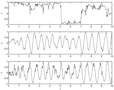
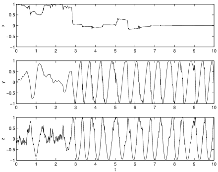
Fig. 1 shows the conditioned evolution for $u=1$. Monitoring the $x$ quadrature tends to make $x$ well-defined (i.e. close to the $\sigma_{x}$ eigenvalues of $\pm 1$). However, it is certainly not perfect in this respect, as large oscillations in $y$ and $z$ due to the rotation around the $x$ axis at rate $\Omega$ are still evident.

FIG. 2.: Non-invariant unraveling with $u=-1$ (homodyne measurement of $y$ quadrature).

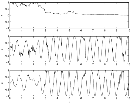
Figure 2 shows the case $u=-1$, which corresponds to a homodyne measurement of the $y$ quadrature of the system, so

$${\rm E}[J(t)]=i\sqrt{\gamma}\,\left\langle{\sigma_{y}}\right\rangle~{}.$$ (55)

The measurement tries to make $y$ well-defined, but fails because the Rabi cycling rotates $y$ into $z$ and so on. Nevertheless, $x$ is forced towards zero, where it stays.

FIG. 3.: Invariant unraveling with $u=0$ (heterodyne detection).

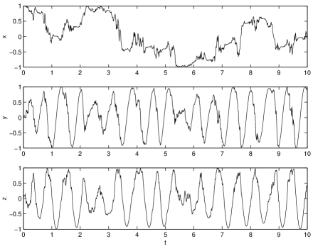
The standard invariant unraveling, or “quantum state diffusion” [10] case of $u=0$ is shown in Fig. 3. This could be realized by heterodyne detection [17], which is like homodyne detection but with a far-detuned local oscillator. This ensures that both quadratures are sampled equally. The current $J$ (which is the complex Fourier transform of the physical photocurrent) has a mean

$${\rm E}[J(t)]=\sqrt{\gamma}\,\left\langle{\sigma}\right\rangle~{}.$$ (56)

The resultant evolution is intermediate between that of $u=1$ and $u=-1$: both $\sigma_{x}$ and $\sigma_{y}$ are being equally monitored, and the result is controlling a certain dynamical feed-back [31].

Next we plot the simulation of the first of our new invariant unravelings. We choose $u$ to be given by Eq. (47), where $R$ is chosen to be the positive number such that $|u|=1$ [the alternative, Eq. (48), simply gives $u=0$ again]. In this case we find $u=-\left\langle{\sigma}\right\rangle/\left\langle{\sigma^{\dagger}}\right\rangle$, so that

$${\rm E}[J(t)]=0~{}.$$ (57)

That is, the current consists purely of white noise. This is not because the monitoring no longer gives any information about the system; it is merely because the the measured quadrature of $\sigma$ is always chosen to be the one that has an instantaneous mean value of zero.

FIG. 4.: Invariant unraveling with $u$ given by Eq. (47) with maximally positive $R$.

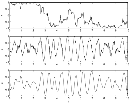
The resultant trajectories are shown in Fig. 4. It appears that the behaviour is qualitatively similar to that of $u=0$. However, note that unlike any of the other cases, the evolution of $z$ is differentiable. This can be proven analytically, since in this case $z$ obeys

$$\dot{z}=-\gamma z-\gamma+\Omega y~{},$$ (58)

which is exactly the same as that obtained from the master equation (50). The evolution of $z$ is of course still stochastic because of the coupling to $y$. This feature is a special case of a general phenomenon noted in Ref. [32], namely that the noise correlations may be chosen to make the evolution of any given operator average smooth.

The final plot, Fig. 5, is for the new invariant unraveling with $u$ given by Eq. (47), where now $R$ is chosen to be the negative number such that $|u|=1$. This gives $u=\left\langle{\sigma}\right\rangle/\left\langle{\sigma^{\dagger}}\right\rangle$ so that

$${\rm E}[J(t)]=\sqrt{\gamma}\,2\left\langle{\sigma}\right\rangle~{}.$$ (59)

In this case the behaviour appears qualitatively similar to that of $u=-1$, in that $x$ is forced to zero. Moreover, the two unravelings becomes equivalent once $x$ reaches $0$, since then $\left\langle{\sigma_{y}}\right\rangle=2\left\langle{\sigma}\right\rangle$. This is interesting, in that an invariant unraveling and a non-invariant unraveling are actually identical in the steady state.

FIG. 5.: Invariant unraveling with $u$ given by Eq. (47) with maximally negative $R$.

VIII Stochastic Schrödinger Equations

We can rewrite the general SME (15) into the form of a SSE (7):

$$d\left|{\psi}\right\rangle=-iH_{\psi}dt\left|{\psi}\right\rangle+\left({c_{k}-\left\langle{c_{k}}\right\rangle}\right)d\xi_{k}^{*}\left|{\psi}\right\rangle~{}.$$ (60)

Using the identity $dP=(d\left|{\psi}\right\rangle)\left\langle{\psi}\right|+\left|{\psi}\right\rangle(d\left\langle{\psi}\right|)+d\left|{\psi}\right\rangle d\left\langle{\psi}\right|$, one can inspect that the above SSE leads to the SME if the nonlinear Hamiltonian is chosen as it follows:

$$-iH_{\psi} = {\cal L}\left|{\psi}\right\rangle\left\langle{\psi}\right|+\mbox{$\frac{1}{2}$}w$$ (61)

$$= -iH-\mbox{$\frac{1}{2}$}\left({c^{\dagger}_{k}c_{k}-2\left\langle{c_{k}}\right\rangle^{*}c_{k}+\left\langle{c_{k}}\right\rangle^{*}\left\langle{c_{k}}\right\rangle}\right)~{}.$$ (62)

It is remarkable that $H_{\psi}$, apart from irrelevant c-number terms, does not depend on the particular representation of the master equation. This is obvious from Eq. (61). Let us re-group its terms in the following ways:

$$H_{\psi}= H+\mbox{$\frac{1}{2}$}\left({i\left\langle{c_{k}}\right\rangle^{*}c_{k}+{\rm H.c.}}\right)$$ (64)

$$-\mbox{$\frac{i}{2}$}\left({c_{k}-\left\langle{c_{k}}\right\rangle}\right)^{\dagger}\left({c_{k}-\left\langle{c_{k}}\right\rangle}\right)~{}.$$

The second term on the r.h.s. is a nonlinear Hermitian term, a kind of mean-field potential. It is invariant under the rotation (2) and its change under the shift (3) exactly cancels the change in $H$. The third term is nonlinear and non-Hermitian, it is responsible for the localization of the wavefunction as a result of continuous monitoring. It is obviously invariant under both transformations (2) and (3).

The invariance of $H_{\psi}$ is a nice feature of the SSE (60), but it must be emphasized that it is not a required property of a SSE. That is because the mapping from SME to SSE is not unique, since a gauge (global phase) transformation

$$\left|{\psi(t)}\right\rangle\to e^{i\chi(t)}\left|{\psi(t)}\right\rangle=\left|{\phi(t)}\right\rangle$$ (65)

does not change the projector $P=\left|{\psi}\right\rangle\left\langle{\psi}\right|=\left|{\phi}\right\rangle\left\langle{\phi}\right|$. For a non-stochastic Schrödinger equation, this transformation will cause only trivial changes to its equation of motion; it will simply add a c-number to the Hamiltonian. However for a SSE it can radically change the equation. This has been noted before (see for example Ref. [33]), but for completeness we show it explicitly.

Consider the case $K=1$ so that we have one complex noise process $d\xi$, and one Lindblad operator $c$ which we will take to be Hermitian and write as $x$. Then the SSE (60) becomes

$$d\left|{\psi}\right\rangle=\left[{-iH-\mbox{$\frac{1}{2}$}\left({x-\left\langle{x}\right\rangle}\right)^{2}}\right]dt\left|{\psi}\right\rangle+\left({x-\left\langle{x}\right\rangle}\right)d\xi^{*}\left|{\psi}\right\rangle~{}.$$ (66)

Now let the global phase obey the equation

$$d\chi=f(t)d\xi^{*}+{\rm c.c.}~{},$$ (67)

where $f(t)$ is an arbitrary smooth function of time. Then

$$\left|{{\phi}}\right\rangle+d\left|{{\phi}}\right\rangle=\left({1+id\chi-\mbox{$\frac{1}{2}$}d\chi d\chi}\right)e^{i\chi(t)}\left({\left|{\psi}\right\rangle+d\left|{\psi}\right\rangle}\right)~{}.$$ (68)

The resultant equation for $\left|{\phi}\right\rangle$ is

$$d\left|{\phi}\right\rangle = \left[{-iH-{\rm Re}\left({f^{2}u^{*}+|f|^{2}}\right)}\right]dt\left|{\phi}\right\rangle$$ (71)

$${-}\mbox{$\frac{1}{2}$}\left({x-\left\langle{x}\right\rangle}\right)\left({x-\left\langle{x}\right\rangle+ifu^{*}+if^{*}}\right)dt\left|{\phi}\right\rangle$$

$${+}\left[{\left({x-\left\langle{x}\right\rangle+if}\right)d\xi^{*}+if^{*}d\xi}\right]\left|{\phi}\right\rangle~{}.$$

Clearly the deterministic part of this is different from Eq. (66), and not invariant.

In this case the transformed equation seems far less appealing in form than the original. However, one can find different forms of the general SSE (60) which, while not having an invariant $H_{\psi}$, have other attractions. In particular, consider the non-unitary gauge transformation defined by

$$\left|{\psi(t)}\right\rangle\to e^{i\chi(t)}\left|{\psi(t)}\right\rangle=\left|{\bar{\phi}(t)}\right\rangle~{},$$ (72)

where $\chi$ is the complex function obeying

$$id\chi=\left\langle{c_{j}}\right\rangle d\xi^{*}_{j}-\mbox{$\frac{1}{2}$}u_{jk}^{*}\left\langle{c_{j}}\right\rangle\left\langle{c_{k}}\right\rangle dt+\mbox{$\frac{1}{2}$}\left\langle{c_{j}}\right\rangle^{*}\left\langle{c_{j}}\right\rangle dt~{}.$$ (73)

The state $\left|{\bar{\phi}}\right\rangle$ is not normalized, which is why it is indicated with an overbar. This is not important, however, as the projector can be defined as $P=\left|{\bar{\phi}}\right\rangle\left\langle{\bar{\phi}}\right|/\left\langle{\bar{\phi}}\right|\left.{\bar{\phi}}\right\rangle$, and this will still obey the SME.

Following the same method as above, one finds that $\left|{\bar{\phi}}\right\rangle$ obeys the SSE

$$d\left|{\bar{\phi}}\right\rangle = dt\left({-iH-\mbox{$\frac{1}{2}$}c^{\dagger}_{k}c_{k}+J^{*}_{k}c_{k}}\right)\left|{\bar{\phi}}\right\rangle$$ (74)

where it is the normalized state $P$ that is used to define the quantum averages in the expression (29) for the currents $J_{k}$. This SSE has a number of nice features. First, it is as simple as the invariant version (60). Second, it very clearly shows the conditioning of the state on the measurement result, and is closely related to the measurement operators (30). Third, it is an easy form to use for numerical calculation (and was in fact used for the simulations in Sec. VII).

IX Discussion

In this paper we have presented new results, and corrected and clarified old results, pertaining to diffusive unravelings of Markovian quantum system dynamics.

First, we have given for the first time the most general form of diffusive quantum unravelings, in Sec. IV. While Gisin restricted his early work [5] for the two-dimensional special case, there have been recent publications which claim to do much the same thing, but in fact do not do so. For example, the recent work of Adler [34] is restricted to Lindblad operators that are Hermitian. Dorsselaer and Nienhuis [35] give a general SSE for a master equation with one Wiener noise term $d\xi$, but for generalizing to the set $\left\{{d\xi_{k}}\right\}_{k=1}^{K}$ they say “we have to assume that the different $d\xi_{k}$ are uncorrelated”. As we have shown here, this is not a necessary assumption; $d\xi_{j}d\xi_{k}=u_{jk}dt$ may be nonzero for $j\neq k$. The non-Hermitian correlation matrix ${\bf u}$ was introduced by one of us and Vaccaro [23], where it was stated that $\forall j,k\,|u_{jk}|\leq 1$. While this is a necessary condition, it is not sufficient. Here we have shown that a necessary and sufficient condition is that the norm $\|{\bf u}\|$ be bounded above by unity.

Second, we have given for the first time the relation between the most general unraveling, as parameterized by ${\bf u}$, and quantum measurement theory. The measurement results which condition the system and so unravel the master equation are $K$ complex “currents” (continuous functions of time) given explicitly in Sec. V. The measurement interpretation of the diffusive unravelings is significant in that it means that the ensembles of pure states resulting from the unraveling can be physically realized. Physical realizability was proposed in Ref. [23] as one of the requirements (along with maximal robustness) for finding the “most natural” ensemble of pure states to represent the mixed state of an open quantum system. Our present work is significant for this program (continued in Ref. [36]) of investigating decoherence in that gives a simple boundary ($\|{\bf u}\|\leq 1$) to the parameter space $\left\{{\bf u}\right\}$ of all diffusive unravelings.

Third, we have corrected the long-standing conception [25, 10, 21] that the only invariant unraveling is the standard diffusive unraveling with ${\bf u}={\bf 0}$. Here invariant means invariance under the linear transformations of the Lindblad and Hamiltonian operators which leave the master equation invariant. In Sec. VI we constructed some explicit examples of invariant unravelings with non-zero ${\bf u}$. The most natural ones have a state-dependent ${\bf u}$ satisfying $\|{\bf u}\|=1$. We illustrated two of these, along with the standard invariant unraveling and some non-invariant unravelings, by numerical simulations of resonance fluorescence in Sec.VII. One of the new schemes produced quite distinctive dynamics for the atom, which ties into recent work on minimizing statistical errors in ensemble average simulations using quantum trajectories [32]. “Quantum state diffusion theory” [10] suggests the standard unraveling as the “most natural”. The existence of non-standard invariant unravelings calls for additional arguments. Recently one of us and Kiefer [37] have applied robustness criteria (different from those in Ref. [23]) to open system unravelings and have approved the standard one.

Fourth, in Sec. VIII we have clarified the notion of invariance in the context of stochastic Schrödinger equations (SSEs) as a way of representing quantum trajectories. It turns out that gauge transformations can radically alter the structure of a given SSE. In particular, the invariance of the standard unraveling is completely destroyed in a generic gauge. This suggests that the best way conceptually to represent quantum trajectories is as a stochastic master equation (SME) for the state projector rather than a SSE for the state vector. Gauge freedom may, on the other hand, allow for equivalent SSEs with different attractions, as demonstrated. The SSEs may be given priority over the SME in numerical calculations, but it must be ensured that all theoretical claims do not rely on non-gauge-invariant properties.