Electroweak Corrections and EFT Operators in $W^{+}W^{-}$ production at the LHC

Abstract

We investigate the impact of electroweak corrections and Effective Field Theory operators on $W^{+}W^{-}$ production at the Large Hadron Collider (LHC). Utilising the Standard Model Effective Field Theory (SMEFT) framework, we extend the Standard Model by incorporating higher-dimensional operators to encapsulate potential new physics effects. These operators allow for a model-independent approach to data interpretation, essential for probing beyond the Standard Model physics. We generate pseudo data at the next-to-leading order in Quantum Chromodynamics and include approximate electroweak corrections. Our analysis focuses on the interplay between these corrections and SMEFT operators at leading order. The inclusion of electroweak corrections is crucial as they can counteract the effects predicted by SMEFT operators, necessitating precise theoretical and experimental handling. By examining $pp\rightarrow W^{+}W^{-}$ production, a process sensitive to the electroweak symmetry-breaking mechanism, we demonstrate the importance of these corrections in isolating and interpreting new physics signatures. Our results highlight the significant role of electroweak corrections in enhancing the interpretative power of LHC data and in obtaining reliable constraints on new physics interactions.

1 Introduction

In the pursuit of deepening our understanding of fundamental interactions and particles, high-energy physics experiments at the Large Hadron Collider (LHC) continue to be a cornerstone of modern physics. As the LHC progresses into its high-luminosity phase (HL-LHC) [1], the sheer volume of data expected necessitates a sophisticated approach to interpretation that is both model-independent and robust. An agnostic methodology based on effective operators offers a promising path to interpreting complex data sets. This approach, crucial for probing beyond the Standard Model (BSM) physics, allows for a comprehensive analysis without relying on specific, potentially unverified extensions of the Standard Model of particle physics (SM). The effective operator framework is instrumental in disentangling new physics signatures from the SM backgrounds, ensuring that our interpretations remain grounded in the data rather than predisposed theoretical models.

The Standard Model Effective Field Theory (SMEFT) (See Refs. [2, 3, 4, 5, 6] and the references therein) provides a systematic framework to incorporate potential deviations from the SM predictions. SMEFT extends the SM by including higher-dimensional operators that encapsulate potential new physics effects at energies beyond the direct reach of current experiments. These operators, which respect the gauge invariance of the SM, parameterise deviations in theory observables in terms of coefficients that are fitted using experimental data. This framework ensures consistency with known physics and remains sensitive to a wide array of possible new phenomena.

As the precision of measurements at the HL-LHC enhances, it becomes increasingly crucial to account for electroweak corrections in the analysis [7]. The large datasets obtained allow for unprecedented detail in measuring the parameters of the SM and beyond, including those modelled by SMEFT. Electroweak corrections, which include contributions from loops involving $W$-, $Z$-bosons, the Higgs particle, and quarks, play a significant role in these measurements. Crucially, the impact of including electroweak corrections may counteract the effects predicted by SMEFT operators. This interplay necessitates careful consideration of these corrections to accurately isolate and interpret the subtle signatures of new physics embedded within the LHC data. Such precision in the theoretical predictions and their experimental verification is indispensable for advancing our understanding of the fundamental constituents of nature.

In this study, we focus on one process, serving as a standard candle for probing the electroweak sector at the LHC. This process, $pp\to W^{+}W^{-}$, is paramount to the LHC program due to its sensitivity to the electroweak symmetry-breaking mechanism and its pivotal role in the precision tests of the SM. Thus, this process offers a robust platform to observe the interplay between electroweak corrections and the effects of new physics as parameterised by SMEFT operators. The $W^{+}W^{-}$ channel has been studied extensively both in the context of the SM as well as beyond [8, 9, 10, 11, 12, 13, 14, 15, 16, 17, 18, 19, 20, 21] both for the LHC and the past and future $e^{+}e^{-}$ colliders. By examining this process at high energies, we aim to demonstrate how electroweak corrections can counter the modifications introduced by SMEFT operators at leading order (LO), thereby highlighting the critical need for precise theoretical and experimental handling of such corrections. This detailed scrutiny is essential for disentangling potential new physics from SM backgrounds and for enhancing the interpretative power of the LHC’s vast datasets.

Our work is structured in the following manner. In Sec. 2 we summarise the importance of the high energy primaries and discuss the SMEFT operators at play. We discuss how our Monte Carlo events are generated with next-to-leading order (NLO) QCD and electroweak corrections in Sec. 3. We validate our SM $W^{+}W^{-}$ results against CMS and perform a fast detector simulation in Sec. 4. We perform a careful statistical analysis and show our results in Sec. 5. Finally, we conclude in Sec. 6.

2 The $pp\to W^{+}(\ell^{+}\nu)W^{-}(\ell^{-}\bar{\nu})$ process in dimension-6 SMEFT

It is possible to probe the effects of the higher-dimensional operators at both low and high energy processes. The low-energy probes include several Higgs couplings which are measured from the run-1 LHC data. These processes, with relatively large cross-sections, have the main disadvantage of being limited by large systematic uncertainties, which are the norm in hadron colliders. The improvement to such coupling measurements will thus not improve drastically even with the accumulation of more integrated luminosity. On the other hand, high-energy probes can be used to constrain leading-order higher-dimensional operators which can give rise to quadratic growth in the centre-of-mass energy ($E$) of some differential distributions in some scattering processes, with respect to SM. If one can measure such energy growing behaviour carefully, the SMEFT effects may be able to trump the systematic uncertainties [22]. In this section, we follow the notations of Refs. [23, 24]. In Tab. 1, we list the operators which contribute to the $pp\to W^{+}W^{-}$ channel at high energies. Even though there are many more operators which contribute to this process, however at high energies, the four deformations $Z_{\mu}\bar{u}_{L/R}\gamma^{\mu}u_{L/R}$ and $Z_{\mu}\bar{d}_{L/R}\gamma^{\mu}d_{L/R}$ are isolated in the dimension-6 deformed Lagrangian. In Ref. [23], it was first pointed out that the same four SMEFT directions (termed the “high energy primaries”) also control the $Zh$ [24], $Wh$ [24, 25] and $WZ$ [23] production channels. At high energies, these four channels correspond to the pair production of the different components of the Higgs doublet owing to the Goldstone Boson Equivalence Theorem [26]. These four processes are thus intertwined through the $SU(2)_{L}$ symmetry for $E>m_{V}^{2}$ ($V=W^{\pm},Z$ boson). At high energies, these four seemingly different processes from the point of view of collider physics, are intricately related. This helps us understand the relation between the pseudo-observables in $W^{+}W^{-}$ production (like the charged triple gauge couplings (cTGCs)) [23, 27] with those in $Vh$ production [24, 28, 25]. A combination of the $Zh$ and the $WZ$ productions was first shown in Ref. [24]. These four channels are also related to the weak-boson fusion channel as shown in Ref. [29].

SILH basis	Warsaw basis
$\mathcal{O}_{W}=\frac{ig}{2}(H^{\dagger}\sigma^{a}\overleftrightarrow{D}^{\mu}H)D^{\nu}W_{\mu\nu}^{a}$	$\mathcal{O}_{L}^{(3)}=(\bar{Q}_{L}\sigma^{a}\gamma^{\mu}Q_{L})(iH^{\dagger}\sigma^{a}\overleftrightarrow{D}_{\mu}H)$
$\mathcal{O}_{B}=\frac{ig^{\prime}}{2}(H^{\dagger}\overleftrightarrow{D}^{\mu}H)\partial^{\nu}B_{\mu\nu}^{a}$	$\mathcal{O}_{L}=(\bar{Q}_{L}\gamma^{\mu}Q_{L})(iH^{\dagger}\overleftrightarrow{D}_{\mu}H)$
$\mathcal{O}_{HW}=ig(D^{\mu}H)^{\dagger}\sigma^{a}(D^{\nu}H)W_{\mu\nu}^{a}$	$\mathcal{O}_{R}^{u}=(\bar{u}_{R}\gamma^{\mu}u_{R})(iH^{\dagger}\overleftrightarrow{D}_{\mu}H)$
$\mathcal{O}_{HB}=ig(D^{\mu}H)^{\dagger}(D^{\nu}H)B_{\mu\nu}$	$\mathcal{O}_{R}^{d}=(\bar{d}_{R}\gamma^{\mu}d_{R})(iH^{\dagger}\overleftrightarrow{D}_{\mu}H)$
$\mathcal{O}_{2W}=-\frac{1}{2}(D^{\mu}W_{\mu\nu}^{a})^{2}$
$\mathcal{O}_{2B}=-\frac{1}{2}(\partial^{\mu}B_{\mu\nu})^{2}$

Table 1: Table shows dimension-6 operators contributing to the high energy longitudinal diboson production channels in the SILH and Warsaw bases.

Coming to the $VV$ and $Vh$ processes ($V=W^{\pm},Z$ boson), the amplitudes scale differently for the different combinations of the longitudinally and transversely polarised gauge bosons when comparing between the SM and BSM contributions. We tabulate the various combinations in Tab. 2 [23]. In this study, we will focus on the longitudinally polarised $W$-boson pair.

	SM	SMEFT
$q_{L/R}\bar{q}_{L/R}\to V_{L}V_{L}(V_{L}h)$	$\sim 1$	$\sim E^{2}/\Lambda^{2}$
$q_{L/R}\bar{q}_{L/R}\to V_{\pm}V_{L}(V_{\pm}h)$	$\sim m_{W}/E$	$\sim m_{W}E/\Lambda^{2}$
$q_{L/R}\bar{q}_{L/R}\to V_{\pm}V_{\pm}(V_{\pm}h)$	$\sim m_{W}^{2}/E^{2}$	$\sim E^{2}/\Lambda^{2}$
$q_{L/R}\bar{q}_{L/R}\to V_{\pm}V_{L}(V_{\pm}h)$	$\sim 1$	$\sim 1$

Table 2: Scaling factors of the di-boson amplitudes for transverse ($\pm$) and longitudinal ($L$) polarisations for the SM and SMEFT scenarios. $\Lambda$ is assumed to be the cut-off scale for new physics.

The BSM Lagrangian in the broken phase can be written as follows [23].

$$\Delta\mathcal{L}_{\textrm{BSM}} =\delta g^{Z}_{uL}\left[Z^{\mu}\bar{u}_{L}\gamma_{\mu}u_{L}+\frac{\cos\theta_{W}}{\sqrt{2}}(W^{+\mu}\bar{u}_{L}\gamma_{\mu}d_{L}+\textrm{h.c.})+\ldots\right]+\delta g^{Z}_{uR}\left[Z^{\mu}\bar{u}_{R}\gamma_{\mu}u_{R}\right]$$

$$+\delta g^{Z}_{dL}\left[Z^{\mu}\bar{d}_{L}\gamma_{\mu}d_{L}-\frac{\cos\theta_{W}}{\sqrt{2}}(W^{+\mu}\bar{u}_{L}\gamma_{\mu}d_{L}+\textrm{h.c.})+\ldots\right]+\delta g^{Z}_{dR}\left[Z^{\mu}\bar{d}_{R}\gamma_{\mu}d_{R}\right]$$ (2.1)

$$+ig\cos{\theta_{W}}\delta g_{1}^{Z}\left[Z^{\mu}(W^{+\nu}W_{\mu\nu}^{-}-\textrm{h.c.})+Z^{\mu\nu}W_{\mu}^{+}W_{\nu}^{-}+\ldots\right]$$

$$+ie\delta\kappa_{\gamma}[(A_{\mu\nu}-\tan{\theta_{W}}Z_{\mu\nu})W^{+\mu}W^{-\nu}+\ldots],$$

with $Z_{\mu\nu}\equiv\hat{Z}_{\mu\nu}-iW^{+}_{[\mu}W^{-}_{\nu]}$, $A_{\mu\nu}\equiv\hat{A}_{\mu\nu}$, $W_{\mu\nu}^{\pm}\equiv\hat{W}_{\mu\nu}^{\pm}\pm iW^{\pm}_{[\mu}(A+Z)_{\nu]}$, where $\hat{V}_{\mu\nu}=\partial_{\mu}V_{\nu}-\partial_{\nu}V_{\mu}$, and $\theta_{W}$ is the Weinberg angle. The ‘$\ldots$’ refers to the Higgs coupling which we do not explicitly consider in this study [30, 24]. In Tab. 2 of Ref. [23] the relations between the high energy primaries (denoted by $a_{q}^{(1)},a_{q}^{(3)},a_{u}$, and $a_{d}$) are related to the low energy primaries. For the high energy primaries, the Warsaw basis [3] of dimension-6 SMEFT operators gives four independent couplings as follows.

$$a_{u}=4\frac{c^{u}_{R}}{\Lambda^{2}},a_{d}=4\frac{c^{d}_{R}}{\Lambda^{2}},a_{q}^{(1)}=4\frac{c^{(1)}_{L}}{\Lambda^{2}},\;\textrm{and}\;a_{q}^{(3)}=4\frac{c^{(3)}_{L}}{\Lambda^{2}},$$ (2.2)

where the above Wilson coefficients are the coefficients of the operators in Tab. 1. The above parameterisation only holds for weakly-coupled “non-universal” theories which must have a complete set of operators. Example tree-level completions of such “non-universal” theories include models with a heavy $SU(2)_{L}$ triplet vector boson which are coupled to the left-handed fermionic currents and to the Higgs current [23, 24].

3 Event Generation

We generate samples for all relevant processes using S HERPA version 2.2.15 [31]. See [32, 33] for an overview of other available frameworks. Matrix elements are generated by the internal tools A MEGIC++ [34] and C OMIX [35], while virtual QCD 1-loop corrections are evaluated using R ECOLA [36]. The samples are generated at $\mathrm{NLO}$ in QCD using the M C @N LO method as implemented in S HERPA [37, 38]. Event are showered using S HERPA ’s Catani-Seymour dipole based shower (CSS hower ) [39] and hadronised using the cluster fragmentation model implemented in the A HADIC++ module [40, 41]. The underlying event is simulated in S HERPA following the Sjöstrand-Zijl model [42].

We include approximate electroweak (EW) corrections in S HERPA based on [43], which includes infrared subtracted EW 1-loop corrections as additional weights to the respective Born cross sections. In those the event weight is calculated based on the expression

$$\mathrm{d}\sigma_{\mathrm{NLO,EW_{\mathrm{approx}}}}=\big{[}B(\Phi)+V_{\text{EW}}(\Phi)+I_{\text{EW}}(\Phi)\big{]}\mathrm{d}\Phi~{},$$ (3.1)

where $B$ denotes the Born contribution also entering the uncorrected QCD cross section, $V_{\text{EW}}$ is the electroweak virtual corrections at 1-loop accuracy, and $I_{\text{EW}}$ is a generalised Catani-Seymour insertion operator for EW NLO calculations. The latter subtracts all infrared singularities of the virtual corrections. This of course is a fundamentally arbitrary procedure, but should provide a good approximation if electroweak Sudakov logarithms are dominant. We use both R ECOLA [44, 45] and O PEN L OOPS [46] to provide the necessary associated virtual contributions. Alternatively to the additive Eq. (3.1), approximate corrections can be multiplicative or exponential to the Born process. We will consider the difference between the three as a systematic uncertainty of the approximation. We generate the following samples with the following general setup.

Standard Model $pp\to W^{+}(l^{+}\nu)W^{-}(l^{-}\nu)$

We wish to study the production of a $W$ boson pair with opposite charges. This sample simulating the SM process contribution is hence central to our study. We use as renormalisation and factorisation scale the sum of the transverse masses of the two $W$ bosons, i.e.

$$\mu_{R}^{2}=\mu_{F}^{2}=M_{\perp,W^{+}}^{2}+M_{\perp,W^{-}}^{2}$$ (3.2)

The electroweak input parameters are set in the so-called $\alpha(M_{Z})$ scheme, and we set

$$M_{W} =80.385~{}\text{GeV},\;\; M_{Z} =91.1876~{}\text{GeV}$$ (3.3)

$$M_{h} =125~{}\text{GeV}\;\; \alpha_{\text{QED}}^{-1}(M_{Z}) =128.802~{}.$$ (3.4)

The $W$ bosons are decayed leptonically in the narrow width approximation smeared by a Breit-Wigner distribution for the mass of the decay system. We assume the measured partial decay width here. The production of $W^{+}W^{-}$ is simulated with M C @N LO accuracy and we include approximate electroweak corrections as described above. Electroweak corrections including the decayed final state have been studied in [15, 47]. We validate the approximate electroweak corrections between the inputs from O PEN L OOPS and R ECOLA . After the validation, we perform the bulk of our analysis with the R ECOLA -based option. Note we do not include any gluon induced contribution in our analysis.

To this end, in Fig. 1 we illustrate the effect of the electroweak corrections and compare the two inputs, at the example of the invariant mass of the final lepton pair and the transverse momentum of the leading lepton in the event. As expected, electroweak corrections become important at large scales close to the TeV in the dilepton invariant mass. In both distributions, we observe excellent agreement between R ECOLA - and O PEN L OOPS -based approximate corrections, giving us confidence that we can work with just one of the samples for our main analysis.

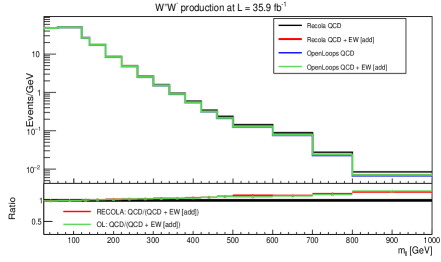
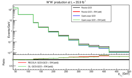
Figure 1: Distribution of the invariant mass of the lepton pair $m_{ll}$ (left) and transverse momentum of the leading lepton $p_{Tl_{1}}$ in $W^{+}W^{-}$ production at a center-of-mass energy of $\sqrt{s}=13~{}\text{TeV}$. Predictions are shown with and without approximate electroweak corrections build from inputs from either O PEN L OOPS or R ECOLA

In order to further investigate the systematics of the approximation, we next study three different schemes to understand the virtual EW corrections. This is shown in Fig. 2. We observe small differences between the schemes, while the qualitative effect remains stable. Quantitatively the effect of the correction is significantly larger than the uncertainty implied by comparing the different schemes.

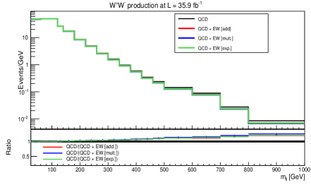
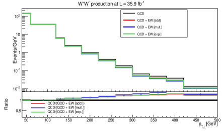
Figure 2: Distribution of the invariant mass of the lepton pair $m_{ll}$ (left) and transverse momentum of the leading lepton $p_{Tl_{1}}$ in $W^{+}W^{-}$ production at a center-of-mass energy of $\sqrt{s}=13~{}\text{TeV}$. Predictions are shown including approximate electroweak corrections in the additive, multiplicative and exponential combination scheme.

SMEFT+SM interference $pp\to W^{+}(l^{+}\nu)W^{-}(l^{-}\nu)$

We use the general UFO [48] interface available in S HERPA [49] to generate samples based on SMEFT in the parametrisation discussed in Sec. 2. We compute the interference between SM and SMEFT at leading order in both QCD and EW. This is then added, at the level of the final histograms, to the $W^{+}W^{-}$ sample described above at NLO QCD and including approximate NLO EW corrections. For the generation of the interference contribution, we assume that SMEFT operators enter in the production of the $W$-boson pair, while for the decays we assume the measured SM branching ratios. We produce separate samples for one of the couplings in the Lagrangian Eq. (2) in Sec. 2, $\delta g^{Z}_{uL}$, $\delta g^{Z}_{uR}$, $\delta g^{Z}_{dL}$, $\delta g^{Z}_{dR}$, set to $1$ while the others are set to $0$. The interference contribution between SM and the SMEFT contribution for the respective part of the Lagrangian is directly proportional to the SMEFT coupling, so the samples can be rescaled to any value of the coupling we need during the analysis, and contributions involving interference of the SM with multiple SMEFT couplings can be obtained by adding the rescaled samples. Note we don’t take terms beyond order $1/\Lambda^{2}$ in the amplitude, so we do not need to produce samples that would involve the product of two or more SMEFT couplings.

Backgrounds

We further simulate samples for the main backgrounds expected. All backgrounds are simulated at M C @N LO accuracy and supplemented with the approximate electroweak corrections as described above. We mostly follow the default settings of the S HERPA Monte Carlo generator, except for when we specify anything different. We include a Drell-Yan (DY) sample for $pp\to\ell^{+}\ell^{-}$ ($\ell^{\pm}=e^{\pm},\mu^{\pm},\tau^{\pm}$) production via a $Z/\gamma^{*}$ $s$-channel exchange. Vector boson production, including merging of higher jet multiplicities, has been studied including approximate electroweak corrections and validated against exact calculations in [50, 43] and electroweak corrections have been studied in [51]. We have separate samples for the production of vector boson pairs other than $W^{+}W^{-}$, i.e., $WZ$ and $ZZ$ pairs, see [52] for a detailed study of electroweak corrections. $W$ production in association with a lepton pair is split into the cases where the $W$ decays either hadronically or leptonically. We also include a sample for top pair $pp\to t\bar{t}$ production where electroweak corrections in the above framework have been studied in [53]. Finally, we consider the production of a top-quark together with a $W$ boson, $pp\to tW$. We did not include the $VVV$ processes in our backgrounds as the contributions are at most 0.6% of the largest background.

4 Analysis and validation against CMS

In order to make our results readily accessible to the readers and to compare against existing experimental analyses, we opt for validating the cut-efficiencies for the SM $q\bar{q}\to W^{+}W^{-}$ sample. For the validation, we mostly follow Ref. [54] . For the object selection criteria, we choose isolated leptons and photons with $p_{T,\ell/\gamma}>10$ GeV, light-jets with $p_{T,j}>30$ GeV, and $b$-tagged jets with $p_{T,b}>20$ GeV. For the electrons and the photons, we require $|\eta(e/\gamma)|<2.5$ barring the barrel-endcap region $1.479<|\eta(e)|<1.566$ for the electron. For the muons and the $b$-tagged jets, we necessitate $|\eta(\mu/b)|<2.4$ and for the light-jets, $|\eta(j)|<4.7$. For the tagging and misindentification efficiencies, we choose a “very loose” working point with $\epsilon_{b\to b}=81\%$, $\epsilon_{c\to b}=42\%$, and $\epsilon_{j\to b}=15\%$ . The electrons (muons) are considered isolated when the sum $p_{T}$ of all the particle flow candidates within a cone radius of $\Delta R=\sqrt{\Delta\eta^{2}+\Delta\phi^{2}}<0.3\;(0.4)$ around it and excluding itself is required to be 6% (15%) of its $p_{T}$. For the isolated photon $\Delta R<0.3$ is chosen and the sum $p_{T}$ of the particle flow candidates is required to be less than 10% of its $p_{T}$. The remainder of the cuts used in our analysis are tabulated in Tab. 3. The variables $m_{\ell\ell}$, $p_{T\ell\ell}$, $p_{T}^{\mathrm{miss}}$ and $p_{T}^{\mathrm{miss,proj}}$ are respectively the invariant mass of the two isolated leptons, the combined transverse momentum of the two-lepton system, the missing transverse momentum, and the projected $p_{T}^{\mathrm{miss}}$. Following Refs. [55] and [56], we identify the isolated lepton closest to $\vec{p}_{T}^{\mathrm{\;miss}}$ in azimuthal angle and compute the difference, $\Delta\phi$. When $\Delta\phi<\pi/2$, $p_{T}^{\mathrm{miss,proj}}=|\vec{p}_{T}^{\mathrm{\;miss}}|\sin{\Delta\phi}|$. For $\Delta\phi\geq\pi/2$, $p_{T}^{\mathrm{miss,proj}}=|\vec{p}_{T}^{\mathrm{\;miss}}|$.

Following Ref. [55], we refer to the final states involving either $ee$ or $\mu\mu$ as same-flavour (SF) and the ones with $e\mu$ as different-flavour (DF). Note that most of the cuts are equal for the SF and DF cases except for three cuts; $m_{\ell\ell}$, $|m_{\ell\ell}-m_{Z}|$, and $\not{E}_{T}$, where $m_{Z}$ is the central value of the observed mass for the $Z$-boson and $\not{E}_{T}$ is the missing transverse energy. The latter two cuts are extremely effective in reducing the enormous DY background.

To validate our setup against CMS, we choose the $q\bar{q}\to W^{+}W^{-}\to 2\ell+\not{E}_{T}$ channel. For the validation, we choose the same sets of cuts for $e\mu$, $\mu\mu$ and $ee$ except for the multivariate DYMVA score which is based on a boosted decision tree. These cuts are tabulated in Tab. 3. While most of our cut efficiencies match within 10% of CMS, there are a few efficiency factors which are different. The ‘two tight leptons’ selection depends on multiple factors including the identification and isolation efficiencies, the differing lepton isolation in the various jet-multiplicity bins, etc. The softer leptons often ensue from the $\tau$-decays and the $\tau$-impact parameter somewhat reduces the lepton $p_{T}$. The electron efficiencies are lower than the corresponding muon ones because of the existing backgrounds. Even though at the reconstruction level, it is very efficient to find electrons and muons, but the full electron selection is much tighter because there are stronger backgrounds to start with. In order to reduce the backgrounds associated with the electron events, the electron efficiency becomes much smaller. Thus, for the ‘two tight leptons’ cut, we impose scale factors of 0.89, 0.34, and 0.56 for the $\mu\mu$, $ee$, and $e\mu$ final states. The $e\mu$ scaling is obtained by taking a square root of the product of the scale factors for the $\mu\mu$ and $ee$ channels.

As for the jet multiplicities in the 0, 1, and $\geq 2$ jet categories, we get $\sim 65:25:10$ in the respective bins. We corroborate this result with the Rivet routine [57] provided by the CMS collaboration for the analysis of [54]. There is another subtlety that we deal with. There is a sizeable fraction of events with no generation-level jets with $p_{T}<30$ GeV. However, these are found at the reconstruction level. These include the effects of jet smearing [55], which we include in our analysis  and the effect of pileup jets which is not included in our generation. Thus, we rescaled the number of reconstructed jet distribution. We use factors of 0.87, 1.38, and 1.78 for 0, 1, and $\geq 2$ jet bins . In Tab. 4, we show the validation of the $q\bar{q}\to W^{+}W^{-}$ channel in the 9 final states.

Within our setup, we also validate the DF scenario for the other SM backgrounds. The major backgrounds are listed in section 3. In Tab. 5, we compare the event numbers of the various backgrounds against Ref. [55]. It is important to note that we did not generate any gluon initiated backgrounds. Hence, we have lesser contribution to the $gg\to ZZ$ and $gg\to W^{+}W^{-}$ backgrounds. The ‘Tops’ ($t\bar{t}+tW$) and DY backgrounds show some deviations due to statistical limitations, which are significant due to the large cross-sections of these processes. The NLO QCD and NLO Electroweak cross-section of $t\bar{t}$ is $\sim 700$ pb and that of DY is $\sim 3100$ pb. We do not validate the other SM backgrounds for the SF scenario because we do not employ the multivariate DYMVA analysis as performed in Ref. [55]. In our high-energy analysis, we impose stronger cuts on the $p_{T}$ of the two leptons and on $m_{\ell\ell}$.

Cut	DF	SF
At least two loose leptons
Exactly two loose leptons
$p_{T_{\ell_{1}/\ell_{2}}}$ [GeV]	20	20
Flavour selection	$e\mu$	$\mu\mu,$ or $ee$
Two tight leptons
Opposite sign leptons
$p_{T_{\ell_{1}}}$ [GeV]	25	25
$p_{T_{\ell_{2}}}$ [GeV]	20	20
$m_{{\ell\ell}}$ [GeV]	20	40
$|m_{{\ell\ell}}-m_{Z}|$ [GeV]	$-$	15
$p_{T_{\ell\ell}}$ [GeV]	30	30
$\not{E}_{T}$ [GeV]	20	55
$\not{E}_{T}^{\mathrm{miss,proj.}}$ [GeV]	20	20
Number of jets	$\leq 1$	$\leq 1$
Number of $b$-tagged jets	0	0

Table 3: Selection criteria for different-flavoured (DF) and same-flavoured (SF) dilepton events following Ref. [54].

Final state	$0-$jets	$1-$jet	$\geq 2-$jets
$e\mu$ [CMS internal]	6632	2953	1348
$e\mu$ [This analysis]	6816	3059	1413
$e\mu$ [54]	$6430\pm 250$	$2530\pm 140$	NA
$\mu\mu$ [CMS internal]	5388	2332	1069
$\mu\mu$ [This analysis]	5508	2554	1175
$\mu\mu$ [54]	NA	NA	NA
$ee$ [CMS internal]	2041	915	434
$ee$ [This analysis]	2076	922	436
$ee$ [54]	NA	NA	NA

Table 4: $q\bar{q}\to WW$ events validation with CMS (internal correspondence) and Ref. [54]. The integrated luminosity for this validation is $\mathcal{L}=35.9\;\textrm{fb}^{-1}.$

Background	$0-$jets	$1-$jet
Tops ($t\bar{t}+tW$) [55]	$2110\pm 110$	$5000\pm 120$
Tops ($t\bar{t}+tW$) [This analysis]	1678	6894
Drell-Yan [55]	$129\pm 10$	$498\pm 38$
Drell-Yan [This analysis]	14	740
$VZ\;(WZ+ZZ)$ [55]	$227\pm 13$	$270\pm 12$
$VZ\;(WZ+ZZ)$ [This analysis]	96	183
$W\ell\ell$ [55]	$147\pm 17$	$136\pm 13$
$W\ell\ell$ [This analysis]	105	197

Table 5: Comparing number of events for the other SM backgrounds between this analysis and [54]. The integrated luminosity for this validation is $\mathcal{L}=35.9\;\textrm{fb}^{-1}.$

5 Results

After validating the $W^{+}W^{-}$ SM channel with CMS in section 4, we want to see the effects of including the NLO EW corrections on the four high-energy primaries. We use 1D and 2D $\chi^{2}$ analyses to show this impact. We take the invariant mass of the two leptons, $m_{\ell\ell}$, as our variable of choice for bounding the four high-energy primaries. Alternatively, we could have used $p_{T_{\ell_{1}}}$, $p_{T_{\ell_{2}}}$, or $\not{E}_{T}$. Given the computational cost of filling the very high energy bins with enough Monte Carlo events, we choose the highest bin as 1 TeV thus totalling 17 bins of non-uniform bin widths. We refer to these bins by $i$. We also ensure that for the same flavour case, where we employ an additional cut of $|m_{{\ell\ell}}-m_{Z}|>15$ GeV, the bin doesn’t split in this range. We have six sub-categories, $j$, per bin, which we refer to as $e\mu-0$, $e\mu-1$, $ee-0$, $ee-1$, $\mu\mu-0$, and $\mu\mu-1$, where ‘0’ and ‘1’ refer to the jet multiplicity. For unweighted events, the statistical uncertainty would go as $\sigma^{\textrm{exp. (theo.)}}_{ij,\textrm{stat.}}=\frac{\sqrt{\hat{N}^{\textrm{exp. (theo.)}}_{ij}}}{\hat{N}^{\textrm{exp. (theo.)}}_{ij}}$, where $\hat{N}^{\textrm{exp. (theo.)}}_{ij}$ is the expected (model) number of events in bin $i$ and sub-category $j$. We perform our analysis at $\mathcal{L}=300$ fb^-1 and at 3 ab^-1. For the full analysis, we assume a flat systematic uncertainty of 5%. For unweighted events, the total uncertainty on the SM prediction for bin $i$ and sub-category $j$ is $\sigma_{ij}=\sqrt{(\sigma^{\textrm{exp.}}_{ij,{\textrm{stat.}}})^{2}+(\sigma^{\textrm{theo.}}_{ij,{\textrm{stat.}}})^{2}+(\sigma^{\textrm{exp.}}_{ij,{\textrm{syst.}}})^{2}+(\sigma^{\textrm{theo.}}_{ij,{\textrm{syst.}}})^{2}}$, where $\sigma^{\textrm{exp. (theo.)}}_{ij,\textrm{syst.}}=0.05\times\hat{N}^{\textrm{exp. (theo.)}}_{ij}$ is the systematic uncertainty for the expected (model) events for the same bin and corresponding sub-category. For weighted events, which is our case, the relative statistical uncertainty for bin $i$ scales as $\sqrt{\Sigma_{k}w_{k}^{2}}/{\Sigma_{k}w_{k}}$, assuming that there is variation of weights within the bin. We perform a $\chi^{2}$ fit with an assumption that the correlations between the different processes are negligible. Our second assumption is based on the fact that our analysis is a future prediction for luminosities which have not yet been reached. We use the following formula.

$$\chi^{2}=\sum_{i}\sum_{j}\frac{[\mathcal{O}^{\textrm{theo.}}_{ij}(p)-\mathcal{O}^{\textrm{exp., SM}}_{ij}]^{2}}{\sigma_{ij}^{2}}$$ (5.1)

Here $\mathcal{O}^{\textrm{theo.}}_{ij}(p)=\mathcal{O}^{\textrm{SM}}_{ij}+p\times\mathcal{O}^{\textrm{SMEFT}}_{ij}$ is calculated for each bin and each sub-category for a coupling $p=\delta g^{Z}_{d_{R}},\delta g^{Z}_{u_{R}},\delta g^{Z}_{u_{L}},$ or $\delta g^{Z}_{d_{L}}$. We must note that while considering the statistical and systematic uncertainties ensuing from the ‘theory’ part, we do not consider the contributions coming from the SMEFT pieces, which are the unknowns that are being extracted from the fit. In this analysis, we are only retaining the interference terms under the assumption that the interference pieces dominate over the squared terms. We are thus also not considering the effects of the cross-terms between the various operators. $\mathcal{O}^{\textrm{exp., SM}}_{ij}$ is computed at NLO QCD + approximate NLO EW, as described in Sec. 3. This is our pseudo data. In Tab. 6, we show the 1D 95% bounds on the four couplings for $\mathcal{L}=300$ fb^-1 and 3 ab^-1. In Fig. 3, we show the bounds on the four parameters at 95% C.L. and compare between the following two scenarios: (i) theoretical model is computed at NLO QCD for SM and SMEFT at LO, and (ii) theoretical model is computed at NLO QCD + approximate NLO EW for SM and SMEFT at LO. We see that the bounds are symmetric about zero when the expected theory is taken at NLO QCD + approximate NLO EW for SM and SMEFT at LO. Only the SMEFT interference piece survives and we get no dependence on the sign of the high-energy primaries. On the other hand, when the expected theory only includes SM computed at NLO QCD and SMEFT at LO, the 95% C.L. bound has a sign dependency as the SM parts of the numerator in the $\chi^{2}$ function do not cancel out completely. It is seen that $\delta g^{Z}_{d_{L}}$ is most strongly constrained. It is important to note that the bound on $\delta g^{Z}_{d_{L}}$ is comparable to the one-parameter fit from Ref. [24]. For the other three high-energy primaries, our bounds are weaker in this analysis. One of the main reasons for that is that we did not venture beyond $m_{\ell\ell}=1$ TeV. Going to even higher energy bins may improve these constraints. We checked that the bounds are strengthening when we go to $m_{\ell\ell}$ beyond 1 TeV. However, the main point of this work is to emphasise that the inclusion of the Electroweak corrections are imperative. Some of the backgrounds being extremely large in cross-section, and are computationally expensive to accurately predict. In Fig. 4, we show the 2-parameter 95% C.L. bounds on pairs of the four high-energy primaries.

Coupling	QCD: $\mathcal{L}=300$ fb-1	QCD+EW: $\mathcal{L}=300$ fb-1	QCD: $\mathcal{L}=3$ ab-1	QCD+EW: $\mathcal{L}=3$ ab-1
$\delta g^{Z}_{d_{R}}$	[-0.2744 0.0531]	[-0.1569, 0.1569]	[-0.1611, -0.0421]	[-0.0567, 0.0567]
$\delta g^{Z}_{u_{R}}$	[-0.0180, 0.0818]	[-0.0474, 0.0474]	[0.0111, 0.0463]	[-0.0167, 0.0167]
$\delta g^{Z}_{d_{L}}$	[-0.0008, 0.0039]	[-0.0023, 0.0023]	[0.0006, 0.0026]	[-0.0010, 0.0010]
$\delta g^{Z}_{u_{L}}$	[-0.3910, 0.0927]	[-0.2383, 0.2383]	[-0.2969, -0.0702]	[-0.1104, 0.1104]

Table 6: 95% C.L. bounds from one-dimensional $\chi^{2}$ fits with the theory prediction to have the SM piece to be computed at QCD or at QCD+EW.

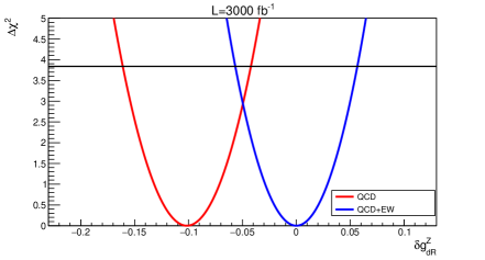
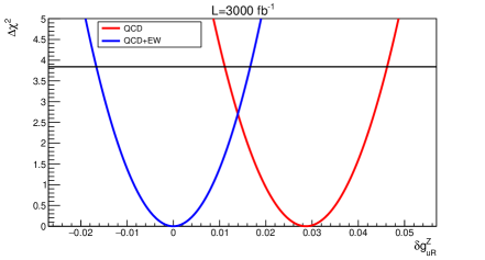
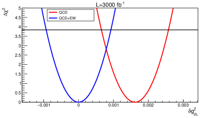
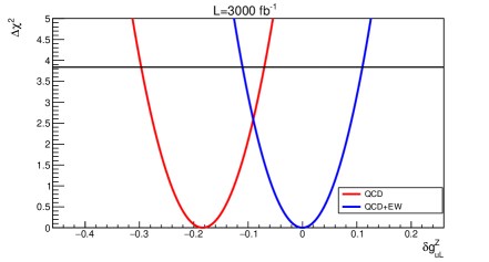
Figure 3: Comparison of the one-dimensional bounds at 95% C.L. between theory assumptions of SM@(NLO QCD) + SMEFT@LO and SM@(NLO QCD + approximate NLO EW) + SMEFT@LO. The expectation assumption is the same, SM@(NLO QCD + approximate NLO EW) for both theory assumptions. The other parameters have not been marginalised over and we consider $\Delta\chi^{2}=3.84$ for a one-parameter $\chi^{2}$ fit to present our allowed regions.

// //

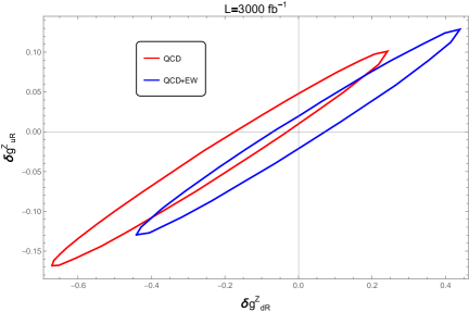
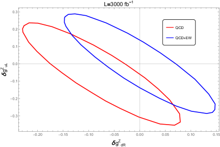
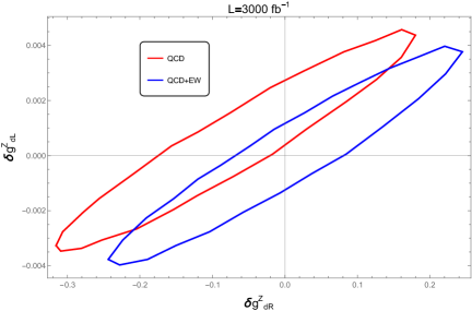
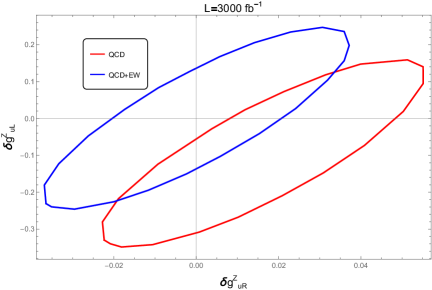
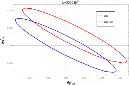
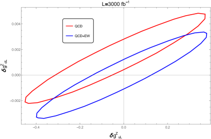
Figure 4: Comparison of the two-dimensional bounds at 95% C.L. between theory assumptions of SM@(NLO QCD) + SMEFT@LO and SM@(NLO QCD + approximate NLO EW) + SMEFT@LO. The expectation assumption is the same, SM@(NLO QCD + approximate NLO EW) for both theory assumptions. The other parameters have not been marginalised over and we consider $\Delta\chi^{2}=5.99$ for a two-parameter $\chi^{2}$ fit to present our contours.

Figs. 3 and 4 show some crucial features. The model assumption is key in deriving and understanding the constraints on the deformations. Given that the HL-LHC will have excellent statistics and a better handle on systematic uncertainties at the end of its run, the model assumption becomes key in understanding the presence of percent or per-mille level deviations or lack thereof. In this exercise, we find that the constraints on the SMEFT parameters, which can be directly linked to constraints on some UV-complete model’s parameters through a top-down matching procedure, depend heavily on our theory assumption. In this case, we can explicitly see that the inclusion of electroweak corrections in the SM part of the theory can drastically alter the allowed regions of new physics. We not only see a shift in the best-fit values, and the allowed ranges, the areas under the two-dimensional contours also change. We see a change between 5 and 9% for the six scenarios. As SMEFT is used as a tool, the directionality of its deformations would point us towards the nature of new physics. Thus, understanding the higher order corrections in our theory observables is imperative. Electroweak corrections become as important as QCD corrections in several bosonic processes, especially in regimes where the energies are much higher than the massive gauge bosons. Depending on the sign of the SMEFT interference contribution, the electroweak corrections can change its bounds.

6 Summary and Outlook

This study investigated the impact of electroweak corrections and EFT operators on $W^{+}W^{-}$ production at the LHC. Utilising the SMEFT framework, we extended the Standard Model to include higher-dimensional operators, providing a model-independent approach to probing potential new physics. Our analysis focused on the interplay between electroweak corrections and SMEFT operators at leading order, demonstrating that electroweak corrections can counteract the effects predicted by SMEFT operators. This interplay necessitates precise theoretical and experimental handling to isolate and interpret new physics signatures accurately. We tensioned the outcome of setting constraints on EFT operators when the background is calculated at NLO QCD accuracy against it being calculated at NLO in QCD and ELW accuracy. Our results highlight the significant role of electroweak corrections in enhancing the interpretative power of LHC data and obtaining reliable constraints on new physics interactions. The $pp\to W^{+}W^{-}$ process served as a benchmark process for this study. Our validation against CMS data confirmed the accuracy and reliability of our theoretical predictions.

This work pioneers incorporating electroweak corrections into SMEFT analyses, emphasising their crucial role in high-energy physics. Future studies should continue to include these corrections in similar analyses, such as $Wh$, $Zh$, $WZ$, and weak-boson fusion processes, to ensure precise isolation and interpretation of new physics effects. The following steps should also extend the SMEFT interference piece to include QCD and approximate electroweak effects. Furthermore, additional improvements should involve studying the relevant operators’ Renormalisation Group Equations [58] and understanding the associated theory systematics. With the High-Luminosity Large Hadron Collider providing unprecedented data volumes, the inclusion of electroweak corrections will become even more critical. The precision in theoretical predictions and their experimental verification will be indispensable for advancing our understanding of the fundamental constituents of nature.

References

- [1] I. Zurbano Fernandez et al., High-Luminosity Large Hadron Collider (HL-LHC): Technical design report 10/2020 (2020), doi:10.23731/CYRM-2020-0010.
- [2] W. Buchmuller and D. Wyler, Effective Lagrangian Analysis of New Interactions and Flavor Conservation, Nucl. Phys. B 268, 621 (1986), doi:10.1016/0550-3213(86)90262-2.
- [3] B. Grzadkowski, M. Iskrzynski, M. Misiak and J. Rosiek, Dimension-Six Terms in the Standard Model Lagrangian, JHEP 10, 085 (2010), doi:10.1007/JHEP10(2010)085, 1008.4884.
- [4] R. Contino, M. Ghezzi, C. Grojean, M. Muhlleitner and M. Spira, Effective Lagrangian for a light Higgs-like scalar, JHEP 07, 035 (2013), doi:10.1007/JHEP07(2013)035, 1303.3876.
- [5] J. Elias-Miró, C. Grojean, R. S. Gupta and D. Marzocca, Scaling and tuning of EW and Higgs observables, JHEP 05, 019 (2014), doi:10.1007/JHEP05(2014)019, 1312.2928.
- [6] I. Brivio and M. Trott, The Standard Model as an Effective Field Theory, Phys. Rept. 793, 1 (2019), doi:10.1016/j.physrep.2018.11.002, 1706.08945.
- [7] A. Bierweiler, T. Kasprzik, J. H. Kühn and S. Uccirati, Electroweak corrections to W-boson pair production at the LHC, JHEP 11, 093 (2012), doi:10.1007/JHEP11(2012)093, 1208.3147.
- [8] K. Hagiwara, R. D. Peccei, D. Zeppenfeld and K. Hikasa, Probing the Weak Boson Sector in e+ e- — W+ W-, Nucl. Phys. B 282, 253 (1987), doi:10.1016/0550-3213(87)90685-7.
- [9] A. Falkowski and F. Riva, Model-independent precision constraints on dimension-6 operators, JHEP 02, 039 (2015), doi:10.1007/JHEP02(2015)039, 1411.0669.
- [10] T. Gehrmann, M. Grazzini, S. Kallweit, P. Maierhöfer, A. von Manteuffel, S. Pozzorini, D. Rathlev and L. Tancredi, Production at Hadron Colliders in Next to Next to Leading Order QCD, Phys. Rev. Lett. 113(21), 212001 (2014), doi:10.1103/PhysRevLett.113.212001, 1408.5243.
- [11] G. Amar, S. Banerjee, S. von Buddenbrock, A. S. Cornell, T. Mandal, B. Mellado and B. Mukhopadhyaya, Exploration of the tensor structure of the Higgs boson coupling to weak bosons in e+ e- collisions, JHEP 02, 128 (2015), doi:10.1007/JHEP02(2015)128, 1405.3957.
- [12] A. Butter, O. J. P. Éboli, J. Gonzalez-Fraile, M. C. Gonzalez-Garcia, T. Plehn and M. Rauch, The Gauge-Higgs Legacy of the LHC Run I, JHEP 07, 152 (2016), doi:10.1007/JHEP07(2016)152, 1604.03105.
- [13] L. Berthier, M. Bjørn and M. Trott, Incorporating doubly resonant data in a global fit of SMEFT parameters to lift flat directions, JHEP 09, 157 (2016), doi:10.1007/JHEP09(2016)157, 1606.06693.
- [14] B. Biedermann, M. Billoni, A. Denner, S. Dittmaier, L. Hofer, B. Jäger and L. Salfelder, Next-to-leading-order electroweak corrections to 4 leptons at the LHC, JHEP 06, 065 (2016), doi:10.1007/JHEP06(2016)065, 1605.03419.
- [15] S. Kallweit, J. M. Lindert, S. Pozzorini and M. Schönherr, NLO QCD+EW predictions for diboson signatures at the LHC, JHEP 11, 120 (2017), doi:10.1007/JHEP11(2017)120, 1705.00598.
- [16] J. Baglio, S. Dawson and I. M. Lewis, An NLO QCD effective field theory analysis of production at the LHC including fermionic operators, Phys. Rev. D 96(7), 073003 (2017), doi:10.1103/PhysRevD.96.073003, 1708.03332.
- [17] C. Grojean, M. Montull and M. Riembau, Diboson at the LHC vs LEP, JHEP 03, 020 (2019), doi:10.1007/JHEP03(2019)020, 1810.05149.
- [18] J. De Blas, G. Durieux, C. Grojean, J. Gu and A. Paul, On the future of Higgs, electroweak and diboson measurements at lepton colliders, JHEP 12, 117 (2019), doi:10.1007/JHEP12(2019)117, 1907.04311.
- [19] J. J. Ethier, G. Magni, F. Maltoni, L. Mantani, E. R. Nocera, J. Rojo, E. Slade, E. Vryonidou and C. Zhang, Combined SMEFT interpretation of Higgs, diboson, and top quark data from the LHC, JHEP 11, 089 (2021), doi:10.1007/JHEP11(2021)089, 2105.00006.
- [20] Anisha, S. Das Bakshi, S. Banerjee, A. Biekötter, J. Chakrabortty, S. Kumar Patra and M. Spannowsky, Effective limits on single scalar extensions in the light of recent LHC data, Phys. Rev. D 107(5), 055028 (2023), doi:10.1103/PhysRevD.107.055028, 2111.05876.
- [21] R. Aoude, E. Madge, F. Maltoni and L. Mantani, Probing new physics through entanglement in diboson production, JHEP 12, 017 (2023), doi:10.1007/JHEP12(2023)017, 2307.09675.
- [22] C. Englert, R. Kogler, H. Schulz and M. Spannowsky, Higgs characterisation in the presence of theoretical uncertainties and invisible decays, Eur. Phys. J. C 77(11), 789 (2017), doi:10.1140/epjc/s10052-017-5366-8, 1708.06355.
- [23] R. Franceschini, G. Panico, A. Pomarol, F. Riva and A. Wulzer, Electroweak Precision Tests in High-Energy Diboson Processes, JHEP 02, 111 (2018), doi:10.1007/JHEP02(2018)111, 1712.01310.
- [24] S. Banerjee, C. Englert, R. S. Gupta and M. Spannowsky, Probing Electroweak Precision Physics via boosted Higgs-strahlung at the LHC, Phys. Rev. D 98(9), 095012 (2018), doi:10.1103/PhysRevD.98.095012, 1807.01796.
- [25] S. Banerjee, R. S. Gupta, J. Y. Reiness, S. Seth and M. Spannowsky, Towards the ultimate differential SMEFT analysis, JHEP 09, 170 (2020), doi:10.1007/JHEP09(2020)170, 1912.07628.
- [26] M. S. Chanowitz and M. K. Gaillard, The TeV Physics of Strongly Interacting W’s and Z’s, Nucl. Phys. B 261, 379 (1985), doi:10.1016/0550-3213(85)90580-2.
- [27] H. El Faham, G. Pelliccioli and E. Vryonidou, Triple-gauge couplings in LHC diboson production: a SMEFT view from every angle (2024), 2405.19083.
- [28] S. Banerjee, R. S. Gupta, J. Y. Reiness and M. Spannowsky, Resolving the tensor structure of the Higgs coupling to -bosons via Higgs-strahlung, Phys. Rev. D 100(11), 115004 (2019), doi:10.1103/PhysRevD.100.115004, 1905.02728.
- [29] J. Y. Araz, S. Banerjee, R. S. Gupta and M. Spannowsky, Precision SMEFT bounds from the VBF Higgs at high transverse momentum, JHEP 04, 125 (2021), doi:10.1007/JHEP04(2021)125, 2011.03555.
- [30] R. S. Gupta, A. Pomarol and F. Riva, BSM Primary Effects, Phys. Rev. D 91(3), 035001 (2015), doi:10.1103/PhysRevD.91.035001, 1405.0181.
- [31] E. Bothmann et al., Event Generation with Sherpa 2.2, SciPost Phys. 7(3), 034 (2019), doi:10.21468/SciPostPhys.7.3.034, 1905.09127.
- [32] J. M. Campbell et al., Event Generators for High-Energy Physics Experiments, SciPost Phys. 16(5), 130 (2024), doi:10.21468/SciPostPhys.16.5.130, 2203.11110.
- [33] J. Andersen et al., Les Houches 2023: Physics at TeV Colliders: Standard Model Working Group Report (2024), 2406.00708.
- [34] F. Krauss, R. Kuhn and G. Soff, AMEGIC++ 1.0: A Matrix element generator in C++, JHEP 02, 044 (2002), doi:10.1088/1126-6708/2002/02/044, hep-ph/0109036.
- [35] T. Gleisberg and S. Hoeche, Comix, a new matrix element generator, JHEP 12, 039 (2008), doi:10.1088/1126-6708/2008/12/039, 0808.3674.
- [36] B. Biedermann, S. Bräuer, A. Denner, M. Pellen, S. Schumann and J. M. Thompson, Automation of NLO QCD and EW corrections with Sherpa and Recola, Eur. Phys. J. C 77, 492 (2017), doi:10.1140/epjc/s10052-017-5054-8, 1704.05783.
- [37] S. Hoeche, F. Krauss, M. Schonherr and F. Siegert, A critical appraisal of NLO+PS matching methods, JHEP 09, 049 (2012), doi:10.1007/JHEP09(2012)049, 1111.1220.
- [38] Höche, Stefan and Krauss, Frank and Schönherr, Marek and Siegert, Frank, QCD matrix elements + parton showers: The NLO case, JHEP 04, 027 (2013), doi:10.1007/JHEP04(2013)027, 1207.5030.
- [39] S. Schumann and F. Krauss, A Parton shower algorithm based on Catani-Seymour dipole factorisation, JHEP 03, 038 (2008), doi:10.1088/1126-6708/2008/03/038, 0709.1027.
- [40] J.-C. Winter, F. Krauss and G. Soff, A Modified cluster hadronization model, Eur. Phys. J. C 36, 381 (2004), doi:10.1140/epjc/s2004-01960-8, hep-ph/0311085.
- [41] G. S. Chahal and F. Krauss, Cluster Hadronisation in Sherpa, SciPost Phys. 13(2), 019 (2022), doi:10.21468/SciPostPhys.13.2.019, 2203.11385.
- [42] T. Sjostrand and M. van Zijl, A Multiple Interaction Model for the Event Structure in Hadron Collisions, Phys. Rev. D 36, 2019 (1987), doi:10.1103/PhysRevD.36.2019.
- [43] S. Kallweit, J. M. Lindert, P. Maierhofer, S. Pozzorini and M. Schönherr, NLO QCD+EW predictions for V + jets including off-shell vector-boson decays and multijet merging, JHEP 04, 021 (2016), doi:10.1007/JHEP04(2016)021, 1511.08692.
- [44] S. Actis, A. Denner, L. Hofer, A. Scharf and S. Uccirati, Recursive generation of one-loop amplitudes in the Standard Model, JHEP 04, 037 (2013), doi:10.1007/JHEP04(2013)037, 1211.6316.
- [45] S. Actis, A. Denner, L. Hofer, J.-N. Lang, A. Scharf and S. Uccirati, RECOLA: REcursive Computation of One-Loop Amplitudes, Comput. Phys. Commun. 214, 140 (2017), doi:10.1016/j.cpc.2017.01.004, 1605.01090.
- [46] F. Buccioni, J.-N. Lang, J. M. Lindert, P. Maierhöfer, S. Pozzorini, H. Zhang and M. F. Zoller, OpenLoops 2, Eur. Phys. J. C 79(10), 866 (2019), doi:10.1140/epjc/s10052-019-7306-2, 1907.13071.
- [47] S. Bräuer, A. Denner, M. Pellen, M. Schönherr and S. Schumann, Fixed-order and merged parton-shower predictions for WW and WWj production at the LHC including NLO QCD and EW corrections, JHEP 10, 159 (2020), doi:10.1007/JHEP10(2020)159, 2005.12128.
- [48] C. Degrande, C. Duhr, B. Fuks, D. Grellscheid, O. Mattelaer and T. Reiter, UFO - The Universal FeynRules Output, Comput. Phys. Commun. 183, 1201 (2012), doi:10.1016/j.cpc.2012.01.022, 1108.2040.
- [49] S. Höche, S. Kuttimalai, S. Schumann and F. Siegert, Beyond Standard Model calculations with Sherpa, Eur. Phys. J. C 75(3), 135 (2015), doi:10.1140/epjc/s10052-015-3338-4, 1412.6478.
- [50] S. Kallweit, J. M. Lindert, P. Maierhöfer, S. Pozzorini and M. Schönherr, NLO electroweak automation and precise predictions for W+multijet production at the LHC, JHEP 04, 012 (2015), doi:10.1007/JHEP04(2015)012, 1412.5157.
- [51] J. M. Lindert et al., Precise predictions for jets dark matter backgrounds, Eur. Phys. J. C 77(12), 829 (2017), doi:10.1140/epjc/s10052-017-5389-1, 1705.04664.
- [52] E. Bothmann, D. Napoletano, M. Schönherr, S. Schumann and S. L. Villani, Higher-order EW corrections in ZZ and ZZj production at the LHC, JHEP 06, 064 (2022), doi:10.1007/JHEP06(2022)064, 2111.13453.
- [53] C. Gütschow, J. M. Lindert and M. Schönherr, Multi-jet merged top-pair production including electroweak corrections, Eur. Phys. J. C 78(4), 317 (2018), doi:10.1140/epjc/s10052-018-5804-2, 1803.00950.
- [54] A. M. Sirunyan et al., W+W- boson pair production in proton-proton collisions at 13 TeV, Phys. Rev. D 102(9), 092001 (2020), doi:10.1103/PhysRevD.102.092001, 2009.00119.
- [55] V. Khachatryan et al., Jet energy scale and resolution in the CMS experiment in pp collisions at 8 TeV, JINST 12(02), P02014 (2017), doi:10.1088/1748-0221/12/02/P02014, 1607.03663.
- [56] P. Fernandez Manteca, W+W- BOSON PAIR PRODUCTION IN PROTON-PROTON COLLISIONS AT CENTER-OF-MASS ENERGY OF WITH THE CMS DETECTOR AT THE LHC. PRODUCCIÓN DE DOS BOSONES W+W- EN COLISIONES PROTÓN-PROTÓN A UNA ENERGÍA DE CENTRO DE MASAS DE CON EL DETECTOR CMS DEL LHC, Presented 21 Jan 2022 (2021).
- [57] G. Gomez-Ceballos, Rivet analyses reference (2020).
- [58] C. Englert and M. Spannowsky, Effective theories and measurements at colliders, Physics Letters B 740, 8–15 (2015), doi:10.1016/j.physletb.2014.11.035.