Integrated optical wave analyzer using the discrete fractional Fourier transform
Abstract
Within the expansive domain of optical sciences, achieving the precise characterization of light beams stands as a fundamental pursuit, pivotal for various applications, including telecommunications and imaging technologies. This study introduces an innovative methodology aimed at reconstructing the Wigner distribution function of optical signals; a crucial tool in comprehending the time-frequency behavior exhibited by these signals. The proposed approach integrates two robust mathematical tools: the discrete realization of fractional Fourier transform, and the propagator of the quantum harmonic oscillator in waveguide arrays. This integration offers a direct and efficient method for characterizing optical signals by reconstructing their Wigner distribution function in the scope of integrated optics. We provide evidence of how having knowledge of the signal propagation amid the phase-space reconstruction, has desirable advantages in respect to only knowing the signal state.
I Introduction
In the realm of physics, the Wigner distribution function [1] holds a crucial role in depicting quantum particle wave functions by utilizing two conjugate variables, such as position and momentum, or number and phase [2, 3, 4]. Its significance transcends quantum mechanics, finding extensive applications in signal processing [5, 6, 7] and classical optics [8, 9, 10], owing to its close association with the Fourier transform.
Introduced in 1980 by Namias using an operator-based approach [11], the continuous fractional Fourier transform notably encompasses the conventional Fourier transform as a specific instance. Inheriting crucial properties from its classical counterpart, the fractional Fourier transform has revealed numerous applications across diverse domains, including signal analysis, pattern recognition, both paraxial and non-paraxial optics, and optical image encryption [12, 13, 14, 15, 16, 17, 18, 19]. Studies from a tomographic perspective have demonstrated that applying the Radon transform to the Wigner distribution function defines the squared modulus of the fractional Fourier transform [20, 21, 22, 23].
In optical models, achieving both the complete and fractional Fourier transforms involves employing sets of lenses [24, 25]. In this setup, an input image undergoes transformation either at the focal point or at an intermediate position along the optical path. However, in discrete and finite scenarios, successful implementation of the fractional Fourier transform has been achieved using waveguide arrays, where the coupling between adjacent waveguides is governed by the angular momentum operator [26]. Among various implementations of the discrete fractional Fourier transform [27, 28, 29, 30], we specifically selected this operational approach to perform tomographic reconstructions of the Wigner distribution function. In this context, finite or semi-infinite waveguide arrays (integrated optics) have been situated within the realm of classical-quantum analogies, opening doors to pioneering investigations into phenomena governed by quantum theory [31, 32, 33, 34, 35, 36, 37]. Within this framework, our study unfolds by identifying the discrete harmonic oscillator in terms of the angular momentum operator and, notably, recognizing its propagator as the discrete fractional Fourier transform.
However, as the field is discretely diffracted along the propagation distance until completely recovered after a complete period, a new question arises: Can we take this as a sinogram (or a parallel projection) in the Radon sense? The sense is where rows are detector position numbers along a line, and columns are angles; so it is possible to perform filtered back projections to obtain a discrete version of the Wigner distribution function of the input field. This is no other thing but using parallel projection tomographic techniques. So, the answer is yes, with some cautions on the scale factor side of the final representation of the WDF [21]. We emphasize, albeit the calculation of a conjugate variables’ joint phase-space can be done directly having knowledge of the initial wavefunction, there’s an advantage in having their propagation in a related space, like waveguides, where we can preview some features that lead to characteristics inherited to the Wigner function.
The manuscript is organized as follows. In §II we take an account in the construction of the discrete fractional Fourier transform as a discrete realization of the Discrete Quantum Harmonic Oscillator, using the eigenfunctions, and their proper implementation in an evanescent waveguides arrays. Here, we state how the functions that model the propagation of light (and information) propagates along the angular parameter of the discrete transformation. In §III, we implement the Wigner-Radon protocol using the backprojection on the angle-line space spawned by the (discrete fractional) propagation. Here we give some examples of reconstruction of the Wigner function for selected initial wavefunction. Thus, we can respond the question arose above: the discrete fractional Fourier transform can be seeing as a proper sinogram, enabling an analysis of optical profiles. In §IV we give our conclusions and perspectives on the method and protocol proposed in this work.
II Discrete fractional Fourier transform
In this section, we explore the concept of the discrete fractional Fourier transform (DFrFT), which is founded upon a set of eigenvectors associated with the Discrete Quantum Harmonic Oscillator (DQHO), serving as the discrete counterpart to the well-established Hermite-Gauss functions [38, 27, 39]. It is of paramount importance to reiterate that the wavefunction of a Quantum Harmonic Oscillator (QHO) at a time is precisely described by the propagator, as outlined in Appendix A [11, 40, 41],
| (1) |
where is the FT of the initial condition, and
| (2) |
is the transformation kernel, known as the Green’s function of the QHO. Two critical aspects require emphasis: a) Despite the initial condition being set at , the boundary conditions on span all possible points within the configuration space. This leads to the FT of , which essentially represents the initial wave function. b) When time reaches , the kernel of the previous transformation simplifies into the FT. This holds great importance, as it yields fractional orders of the FT within the interval from to .
Within this perspective, it is noteworthy that previous research [26] has shown that a feasible discrete and finite version of the QHO can be derived by considering generators associated with the rotation algebra within a setup of evanescent coupled waveguide arrays, thus defining an odd-dimensional Hilbert space [42, 40]. Vectors in this space, denoted as , possess finite support. Specifically, for given values of and , these vectors have a spectral range extending from to , resulting in a space dimensionality of . In this context, the generators follow the standard commutation relations, i.e., . Thus, we propose the utilization of the following Hamiltonian,
| (3) |
This choice governs not only the system’s entire dynamics but also faithfully replicates the essential characteristics of the QHO. Furthermore, it naturally gives rise to fractional orders of the FT within discrete and finite spaces [26]. Calculating the matrix elements of this Hamiltonian in the diagonal basis of , they can be expressed as follows:
| (4) |
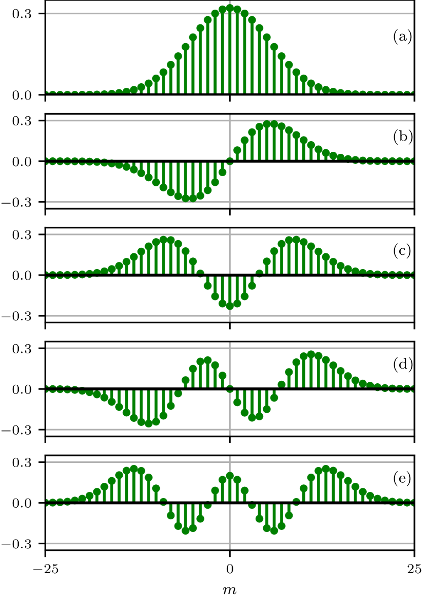
where is a scaling factor. Therefore, we are dealing with odd-dimensional matrices that have off-diagonal elements. In this context, direct diagonalization methods can be employed to obtain the appropriate eigenvector basis of Eq. (3) [42, 26]. Analogously to how Hermite-Gauss polynomials serve as eigenfunctions of the QHO, we can construct eigenvectors for this discrete and finite oscillator using functions that support the requisite indexing. Consequently, the -th component of the resulting eigenfunctions can be expressed as follows:
| (5) |
where represents the Jacobi polynomials of order [42]. In Fig. 1, the first five eigenvectors of the DQHO, Eq. (5), are plotted, illustrating their discrete approximation to the well-known Hermite-Gauss polynomials of the QHO. It is worth noticing that there exists a sort of realizations for the DFrFT, whose count those constructed by 1) sampling the harmonic oscillator eigenfunctions, the “Taipei basi” [43, 44]; 2) sums of periodically displaced oscillator eigenfunctions, the “Metha basis” [45]; 3) the vibrating chain lattice model, the “the Ankara lattice” [46, 28]; 4) and the (2) model of the discrete oscillator, the “Wolf-Fourier-Kravchuk” realization. Despite, every one of these versions of the DFrFT attains some peculiar properties, the use of the realization is chosen as the most closed related to the propagation in waveguides arrays.
With Eq. (1) and Eq. (2) (also refer to Appendix A), we now direct our attention to the dynamic evolution of the DQHO. Naturally, this is governed by a Schrödinger-like equation,
| (6) |
In this context, denotes a vector that is defined in a Hilbert space with dimensions . This serves as a spectral decomposition of the general functions in relation to the basis , and their associated amplitudes . Additionally, we have made a change, without loss of generality, substituting the time variable with a propagation variable . Hence, the remaining challenge lies in devising an efficient method to apply the propagation operator to the initial state vector at ,
| (7) |
Although the propagation operator is given in terms of the angular momentum operator , it is challenging to find a specific representation, since it is a tridiagonal finite matrix given by Eq. (4). In analogy to the Green’s function approach for the QHO Eq. (2), the evolution operator of the DQHO is the DFrFT. Furthermore, a similarity transformation employing the eigenfunctions, as described in Eq. (5), enables the determination of the Green’s function for the DQHO [26, 42],
| (8) |
Similarly to the continuous scenario, the evolution operator coincides with the DFrFT, as expressed by
| (9) |
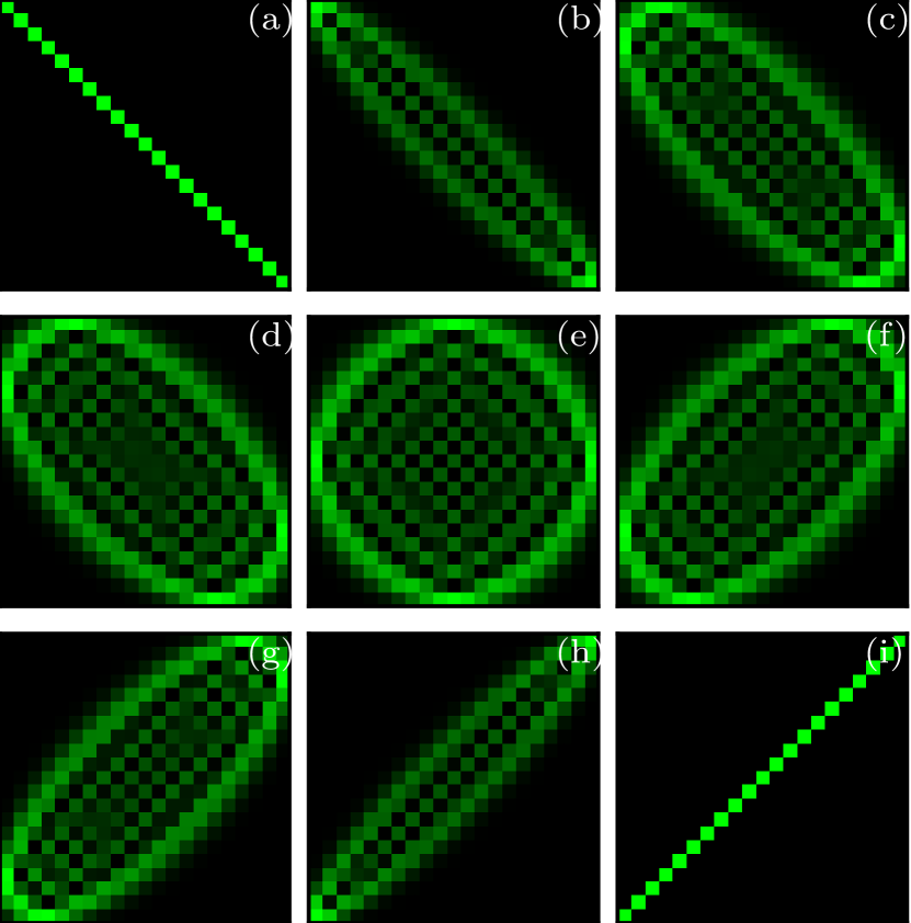
Fig. 2 illustrates the square modulus of the DFrFT for various fractional orders determined by the variable . For each fractional order ranging from to , this provides a transformation of the finite and discrete object within the context of a converging lens. This comprehensive analysis enables a more profound understanding of the optical properties of the system across this range of fractional orders.
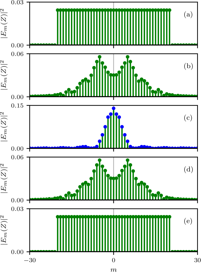
To exemplify the DFrFT operator , we consider a representative scenario where the initial condition is determined by the sampling of a normalized rectangular function as specified in Eq. (7). Subsequently, we generate plots depicting the squared modulus for varying propagation distances. In Fig. 3, it is evident that each discrete value indexed by in the DFrFT at distance is calculated using the following equation:
| (10) |
Where signifies the initial condition. It is worth emphasizing, as previously mentioned, that at , the kernel of the transformation simplifies to the DFT, as showcased in Fig. 3 (d). In the scenario of a one-dimensional rectangular aperture, this leads to a discrete function.
In closing this section, it is imperative to underscore that our ability to obtain the DFrFT extends beyond arbitrary functions; we can also apply it to quantum states. This capability arises from the inherent connection between the evolution operator and the QHO. Theoretically, there are no limitations on the types of initial states we can employ, as long as they meet the requirements of proper sampling and satisfy the Nyquist criterion [47], ensuring the well-defined nature of the DFrFT.
III The Wigner-Radon transform in photonic lattices
The intricacy associated with Wigner function reconstruction via the inverse Radon transform (IRT) primarily stems from the task of obtaining parallel projections [21, 22, 18]. This demanding process necessitates precise alignment and collection of data from various angles, making it a pivotal aspect in the successful retrieval of the WDF. In this section, we use the Radon transform scheme, introduced by Johann Radon [20], where the parallel projections of an object or function of two variables indirectly provide its internal structure. In the specific case of parallel projections of the WDF (function of two variables), these turn out to be the square modulus of the FrFT [21]. Within a discrete and finite framework, the implementation of the DFrFT in photonic arrays hinges on the propagation distance, which dictates the fractional order of the transform [26]. This relationship mirrors the connection observed in the continuous domain between the DQHO and DFrFT.
The RT is an integral transform that arises from the parallel projection of a two-variable function . It is mathematically defined through the following line integral,
| (11) |
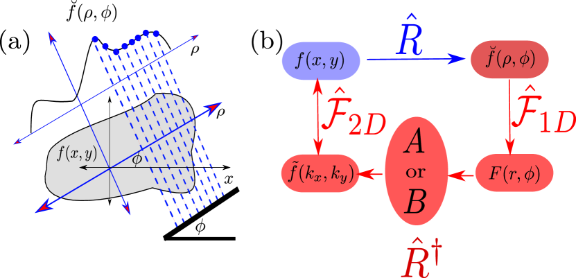
where denotes the action of the RT on the function , represents the abscissa of the rotated system, while denotes the rotation angle (refer to Fig. 4 (a)). Consequently, the number of RT instances corresponds to the number of applied rotation angles. In this regard, Lohmann and Soffer have provided evidence that the FrFT indeed arises from the parallel projections of the WDF [21]. Therefore, applying the RT to the WDF yields the following,
| (12) |
where
| (13) |
represents the integral version of the WDF for a given function . After performing a suitable change in the integration variables, employing Eq. (12) and Eq. (13), Eq. (11) can be expressed in the following manner,
| (14) |
From Eq. (2), we can observe that the previous result can be recognized as the square modulus of the FrFT. This result has been previously demonstrated in [21]. As mentioned earlier, at , the kernel of the transformation corresponds to that of the FT. Furthermore, the projection angle determines each fractional order. Eq. (14) serves as the preamble to our discrete tool for reconstructing the WDF in photonic systems, enabling the characterization and analysis of any discretized signal.
.
Let us now explore the inverse problem, which is tackled by applying the IRT to the square modulus of the FrFT. Two primary approaches are commonly employed to derive the inverse transformation, both rooted in the Fourier Slice Theorem [48, 49], also known as the Central Slice Theorem. In general, the reconstruction of the WDF or any other function requires parallel projections for each angle. As indicated by Eq. (12), when considering one of the possible fractional orders, denoted as , of the FT applied to a function , it becomes possible to derive the following:
| (15) |
In this context, is used to represent the IRT operator, with lying within the range of . Each fractional order corresponds to specific points in the phase space of the WDF. In this regard, the objective of the IRT is to recover or indirectly reconstruct information from a given signal. However, the computational implementation varies depending on the specific objective and is accomplished through various methods [50, 51]: series and orthogonal functions, iterative approaches, direct Fourier methods, as well as signal space convolution and frequency space filtering methods. One of the most straightforward Fourier methods is based on the central slice theorem [52], which establishes a relationship between two-dimensional and one-dimensional Fourier transforms through the RT (as depicted in Fig. 4(b)). Within this framework, it is possible to derive the discrete Wigner distribution (DWDF), either by utilizing the Fourier slice theorem or through the application of filtered back-projection, resulting in
| (16) |
that represents the two-dimensional DFT of the discrete signal , where
| (17) |
Where, and denote points within the phase space, while assumes the role of , where each value of corresponds to a distinct fractional order. Furthermore, signifies the squared modulus of the -th point within the -th fractional order during the sampling process of a function . Here, and are determined by the number of sampling points in the input signal and the number of parallel projections, respectively.
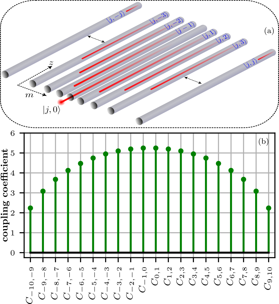
Now, within the discrete and finite framework defined by the DQHO, and considering the scenario of waveguide arrays as governed by the Hamiltonian Eq. (3), we have identified an opportunity for WDF reconstruction. As previously demonstrated, the propagation operator Eq. (9) corresponds to the DFrFT, implying distinct fractional orders for each propagation distance. In the context of the tight-binding limit for a group of waveguides with coupling coefficients defined by (as shown in Fig. 5), the light intensity in each waveguide at a specific propagation distance, (in fractional order), can be expressed by considering a generic initial condition ,
| (18) |
Here can be regarded as the sampling of some function decomposed in the discrete basis, , where represents the amplitudes of the generic sampled signal. Consequently, the light intensity in the -th waveguide undergoes evolution over a distance , and this evolution is determined by the DFrFT operator , as described in Eq. (9). Given that the propagation of light within a waveguide array featuring parabolic-type coupling [26, 53] is governed by the Schrödinger equation, Eq. (6), we can express the evolution of intensity in the array- as a matrix:
| (19) |
To generate each column, a dedicated waveguide array is constructed with the desired propagation distance , and the output intensities in all waveguides are measured. An alternative approach involves doping the waveguides with a suitable fluorescent material and watching the fluorescence intensity along the propagation, with the observation taking place from above the waveguide chip [54]; Fig. 5 (a) represents schematically a finite set of identical evanescent coupled waveguides, where is an integer that determines the dimension of the Hilbert space or the total number of waveguides , while Fig. 5 (b) shows the matrix elements of the angular momentum operator , Eq. (4), that follow a growth of parabolic type. Under these considerations, we are in the possibility of using the DFrFT in a waveguide beam splitter scenario.
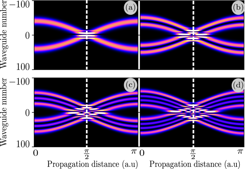
To illustrate the WDF reconstruction process, we will explore four specific scenarios involving the superposition of eigenstates as defined by Eq. (5), which encompass distinct values. Fig. 6 showcases linear combinations or superpositions of states, commonly regarded as Schrödinger cat states [55, 56]. The fractional order in each guide is determined by Eq. (18), which, at , transforms into the discrete integer representation of the initial condition. This transformation, known within the framework of parallel projections, forms the sinogram depicting the studied signal. In the context of the Radon-Wigner transform, the sinogram is defined through the square modulus of the various orders of the fractional discrete Fourier transform (representing the columns in Eq. (19)). These orders are contingent upon the propagation distance . Once all the fractional orders () are obtained, it becomes feasible, employing either the Fourier slice theorem or filtered back-projection techniques, to derive the discrete Wigner distribution. This derivation involves Eqs. (16) and (17). Notably, it’s imperative to recognize that each signifies the intensity in the -the waveguide as a function of the propagation distance (refer to appendix B).
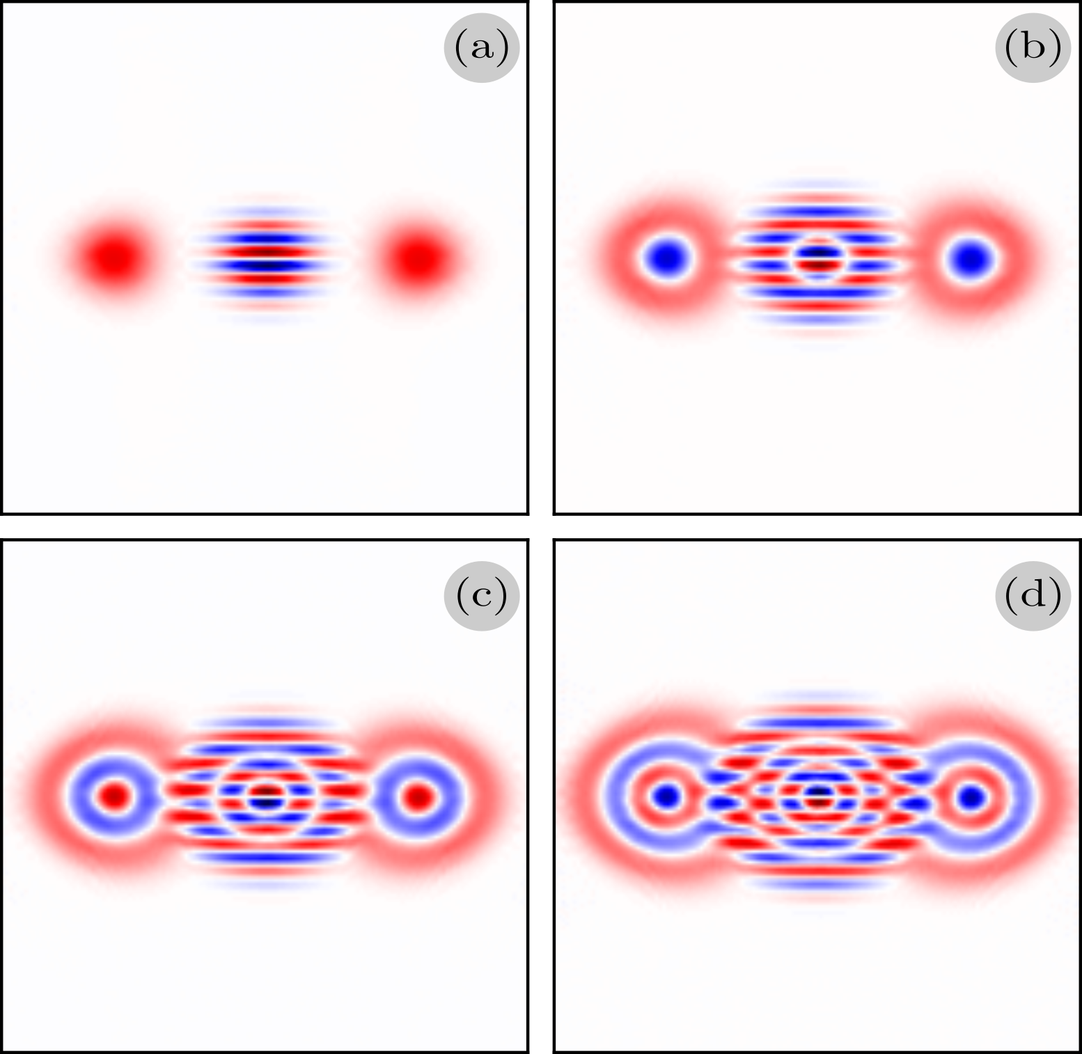
Finally, using Eq. (16) in each of the cases shown in Fig. 6 it is possible to obtain the reconstruction of the discrete Wigner distribution function. In Fig. 7, by using the scikit-image toolbox [57], we have reconstructed the WDF associated with the superposition of eigenstates from QDHO, so-called generalized Schrödinger cat states [56].
IV Conclusions
We have demonstrated that, akin to the continuous case of the quantum harmonic oscillator’s propagator identified as the Fractional Fourier Transform (FrFT), its discrete version accommodates fractional orders of the Discrete Fourier Transform (DFT). This discrete representation, integrated within an array of waveguides marked by lines and angles, allows us to reinterpret the progression of discretized input states as parallel projections conforming to the Radon transform’s framework. Consequently, this reinterpretation facilitates its application within integrated circuits. It’s noteworthy that the discretization of the quantum harmonic oscillator lacks a unique definition, leading to several approaches to obtaining appropriate discrete eigenfunctions that mirror those in the continuous scenario. Nevertheless, each one of these realizations has its scope and applicability. Selecting one, as we do in this work, can respond to the specifics of the system.
The Wigner function, pivotal in signal theory and quantum mechanics, unveils the concurrent time-frequency evolution within a signal. Despite its computationally intricate nature and the challenge in direct interpretation, the Fractional Fourier Transform and the Radon inverse emerge as compelling tools. They facilitate an efficient reconstruction of the Wigner function from data in both the frequency domain and spatial realms, proving pivotal in signal processing and quantum optics. And, as stated at the beginning, and demonstrated with examples, there’s a clear advantage, quantitative and qualitative, to have the propagation of an initial wavefunction, where we can discern features that later will be inherited to the Wigner phase-space.
Moreover, we illustrated the quantum harmonic oscillator’s propagator, conceptualized as a Fractional Fourier Transform (FrFT), finding practical utility in waveguide arrays, such as arrangements resembling . This realization, allows us to reinterpret the evolution of discretized states as projections within the Radon transform framework, simplifying their integration into integrated circuits. It’s notable that discretizing the harmonic oscillator offers multiple approaches to derive discrete functions mimicking its continuous behavior. We hope these findings turn out to be useful for the community who wants to understand the connection between the concepts presented.
Appendix A Continuous fractional Fourier transform
The Schrödinger equation of the quantum harmonic oscillator with , , and , is
| (20) |
and therefore, the wave function at time t is
| (21) |
and using the fact that [40]
| (22) |
in addition to the following relationships
| (23) | ||||
it is possible to obtain that the initial condition evolves as
| (24) |
that when considering the inverse Fourier transform
| (25) |
applied in the initial condition, it is obtained that
| (26) | ||||
The last relation is known as the continuous fractional Fourier transform.
Appendix B The Fourier slice theorem and filtered backprojection
There are two representative numerical methods based on the Fourier slice theorem (Fourier central theorem) and the filtered back-projection to obtain the inverse Radon transform [48, 49]. To accomplish this, let’s define the 2D Fourier transform of as,
| (27) |
while the inverse transform is given by
| (28) |
Therefore, considering polar coordinates
| (29) |
it is possible to obtain that
| (30) | ||||
Thus, a one-dimensional Fourier transform of the FT gives the spectrum, subsequently giving . In our case, the one-dimensional transformation of the parallel projections defined by the Radon transform makes possible the reconstruction of the WDF. Consequently, for the discrete case, we have that the DFT of the parallel projection defined by the distance is
| (31) |
with , and is the -th distance in a range of . Therefore, a point in phase space is determined by the discrete 2D Fourier transform, such that
| (32) | ||||
This relationship summarizes the sketch shown in Fig. 4. Once we obtain the 1D Fourier transform of the projection of any function at a given distance (angle), , we can obtain the Wigner function at any point in the phase space following the same algorithm. Another famous inversion scheme is the Filtered Back projection [49]. It is derived from Eq. (28).
Acknowledgements.
The authors acknowledge the valuable guidance of Armando Pérez-Leija in the early stages of this work. A.R.U. acknowledges support from DGAPA-UNAM posdoctoral program (POSDOC) 2023-2024, and to ICF-UNAM for the in-place support.† This paper is dedicated to the memory of our colleague Dr. Gustavo Rodríguez-Zurita.
References
- Wigner [1932] E. Wigner, On the quantum correction for thermodynamic equilibrium, Phys. Rev. 40, 749 (1932).
- Moya-Cessa [2003] H. Moya-Cessa, A number–phase wigner function, J. Opt. B: Quant. and Semiclass. Opt. 5, S339 (2003).
- Perez-Leija et al. [2016a] A. Perez-Leija, L. A. Andrade-Morales, F. Soto-Eguibar, A. Szameit, and H. M. Moya-Cessa, The pegg–barnett phase operator and the discrete fourier transform, Physica Scripta 91, 043008 (2016a).
- Ramos-Prieto et al. [2020] I. Ramos-Prieto, L. A. Andrade-Morales, F. Soto-Eguibar, and H. M. Moya-Cessa, Pegg–barnett coherent states, J. Opt. Soc. Am. B 37, 370 (2020).
- Bastiaans [1978] M. J. Bastiaans, The Wigner distribution function applied to optical signals and systems, Opt. Commun. 25, 26 (1978).
- Cohen [1989] L. Cohen, Time-Frequency Distributions-A Review (1989).
- Dragoman [2005] D. Dragoman, EURASIP J. Appl. Signal Processing, Vol. 2005 (SpringerOpen, 2005) pp. 1520–1534.
- Bastiaans [1979] M. J. Bastiaans, Wigner distribution function and its application to first-order optics, J. Opt. Soc. Am. 69, 1710 (1979).
- Cho et al. [2009] S. Cho, J. C. Petruccelli, and M. A. Alonso, Wigner functions for paraxial and nonparaxial fields, J. Mod. Opt. 56, 1843 (2009).
- Alonso [2011] M. A. Alonso, Wigner functions in optics: describing beams as ray bundles and pulses as particle ensembles, Adv. Opt. Photonics 3, 272 (2011).
- Namias [1980] V. Namias, The fractional order fourier transform and its application to quantum mechanics, IMA Journal of Applied Mathematics 25, 241 (1980).
- Mendlovic and Ozaktas [1993] D. Mendlovic and H. M. Ozaktas, Fractional Fourier transforms and their optical implementation: I, J. Opt. Soc. Am. A 10, 1875 (1993).
- Ozaktas and Mendlovic [1993] H. M. Ozaktas and D. Mendlovic, Fractional Fourier transforms and their optical implementation II, J. Opt. Soc. Am. A 10, 2522 (1993).
- Ozaktas and Kutay [2001] H. M. Ozaktas and M. A. Kutay, The fractional fourier transform, in 2001 Eur. Control Conf. ECC 2001 (Institute of Electrical and Electronics Engineers Inc., 2001) pp. 1477–1483.
- Almeida [1994] L. B. Almeida, The Fractional Fourier Transform and Time-Frequency Representations, IEEE Trans. Signal Process. 42, 3084 (1994).
- Alieva et al. [1994] T. Alieva, V. Lopez, F. Agullo-Lopez, and L. B. Almeida, The fractional fourier transform in optical propagation problems, J. Mod. Opt. 41, 1037 (1994).
- Lohmann et al. [1996] A. W. Lohmann, Z. Zalevsky, and D. Mendlovic, Synthesis of pattern recognition filters for fractional Fourier processing, Opt. Commun. 128, 199 (1996).
- Tao et al. [2008] R. T. Tao, B. Deng, W. Q. Zhang, and Y. Wang, Sampling and sampling rate conversion of band limited signals in the fractional Fourier transform domain, IEEE Trans. Signal Process. 56, 158 (2008).
- Ramos-Prieto et al. [2023] I. Ramos-Prieto, D. Sánchez-de-la-Llave, U. Ruíz, V. Arrizón, F. Soto-Eguibar, and H. M. Moya-Cessa, Cauchy-riemann beams in grin media (2023), arXiv:2311.09541 [physics.optics] .
- Radon [1986] J. Radon, On the determination of functions from their integral values along certain manifolds., IEEE Trans. Med. Imaging MI-5, 170 (1986).
- Lohmann and Soffer [1994] A. W. Lohmann and B. H. Soffer, Relationships between the Radon–Wigner and fractional Fourier transforms, J. Opt. Soc. Am. A 11, 1798 (1994).
- Wood and Barry [1994] J. Wood and D. Barry, Radon transformation of time-frequency distributions for analysis of multicomponent signals, IEEE Transactions on Signal Processing 42, 3166 (1994).
- Mendlovic et al. [1996] D. Mendlovic, R. G. Dorsch, A. W. Lohmann, Z. Zalevsky, and C. Ferreira, Optical illustration of a varied fractional Fourier-transform order and the Radon–Wigner display, Appl. Opt. 35, 3925 (1996).
- Unnikrishnan et al. [2000] G. Unnikrishnan, J. Joseph, and K. Singh, Optical encryption by double-random phase encoding in the fractional Fourier domain, Opt. Lett. 25, 887 (2000).
- Wang and Cai [2007] F. Wang and Y. Cai, Experimental observation of fractional Fourier transform for a partially coherent optical beam with Gaussian statistics, J. Opt. Soc. Am. A 24, 1937 (2007).
- Weimann et al. [2016] S. Weimann, A. Perez-Leija, M. Lebugle, R. Keil, M. Tichy, M. Gräfe, R. Heilmann, S. Nolte, H. Moya-Cessa, G. Weihs, D. N. Christodoulides, and A. Szameit, Implementation of quantum and classical discrete fractional Fourier transforms, Nat. Commun. 7, 1 (2016).
- Atakishiyev et al. [2005] N. M. Atakishiyev, G. S. Pogosyan, and K. B. Wolf, Finite models of the oscillator (2005).
- Barker et al. [2000] L. Barker, Ç. Candan, T. Hakioglu, M. A. Kutay, and H. M. Ozaktas, The discrete harmonic oscillator, harper's equation, and the discrete fractional fourier transform, Journal of Physics A: Mathematical and General 33, 2209 (2000).
- Jafarov et al. [2011] E. I. Jafarov, N. I. Stoilova, and J. V. der Jeugt, Finite oscillator models: the hahn oscillator, Journal of Physics A: Mathematical and Theoretical 44, 265203 (2011).
- Atakishiyev and Wolf [1997] N. M. Atakishiyev and K. B. Wolf, Fractional fourier–kravchuk transform, Journal of the Optical Society of America A 14, 1467 (1997).
- Christodoulides et al. [2003] D. N. Christodoulides, F. Lederer, and Y. Silberberg, Discretizing light behaviour in linear and nonlinear waveguide lattices, Nature 424, 817 (2003).
- Longhi [2009] S. Longhi, Quantum-optical analogies using photonic structures, Laser & Photonics Reviews 3, 243 (2009), https://onlinelibrary.wiley.com/doi/pdf/10.1002/lpor.200810055 .
- Keil et al. [2011] R. Keil, A. Perez-Leija, F. Dreisow, M. Heinrich, H. Moya-Cessa, S. Nolte, D. N. Christodoulides, and A. Szameit, Classical analogue of displaced Fock states and quantum correlations in Glauber-Fock photonic lattices, Phys. Rev. Lett. 107, 103601 (2011).
- Keil et al. [2012] R. Keil, A. Perez-Leija, P. Aleahmad, H. Moya-Cessa, S. Nolte, D. Christodoulides, and S. A., Observation of bloch-like revivals in semi-infinite glauber–fock photonic lattices, Opt. Lett. 37, 3801 (2012).
- Perez-Leija et al. [2012] A. Perez-Leija, R. Keil, A. Szameit, A. F. Abouraddy, H. Moya-Cessa, and D. N. Christodoulides, Tailoring the correlation and anticorrelation behavior of path-entangled photons in Glauber-Fock oscillator lattices, Phys. Rev. A 85, 013848 (2012).
- Román-Ancheyta et al. [2017] R. Román-Ancheyta, I. Ramos-Prieto, A. Perez-Leija, K. Busch, and R. D. J. León-Montiel, Dynamical Casimir effect in stochastic systems: Photon harvesting through noise, Phys. Rev. A 96, 032501 (2017), arXiv:1706.03838 .
- Ramos-Prieto et al. [2021] I. Ramos-Prieto, K. Uriostegui, J. Récamier, F. Soto-Eguibar, and H. M. Moya-Cessa, Kapitza–dirac photonic lattices, Opt. Lett. 46, 4690 (2021).
- Atakishiev and Suslov [1990] N. M. Atakishiev and S. K. Suslov, Difference analogs of the harmonic oscillator, Theor. Math. Phys. 85, 1055 (1990).
- Candan et al. [2000a] Ç. Candan, M. Alper Kutay, and H. M. Ozaktas, The discrete fractional fourier transform, IEEE Trans. Signal Process. 48, 1329 (2000a).
- Dattoli et al. [1998] G. Dattoli, A. Torre, and G. Mazzacurati, An alternative point of view to the theory of fractional Fourier transform, IMA J. Appl. Math. (Institute Math. Its Appl. 60, 215 (1998).
- Kutay and Ozaktas [2002] M. A. Kutay and H. M. Ozaktas, The fractional Fourier transform and harmonic oscillation, Nonlinear Dyn. 29, 157 (2002).
- Narducci and Orszag [1972] L. M. Narducci and M. Orszag, Eigenvalues and Eigenvectors of Angular Momentum Operator Jx without the Theory of Rotations, Am. J. Phys. 40, 1811 (1972).
- Pei and Yeh [1997] S.-C. Pei and M.-H. Yeh, Improved discrete fractional fourier transform, Optics Letters 22, 1047 (1997).
- Pei et al. [1999] S.-C. Pei, M.-H. Yeh, and C.-C. Tseng, Discrete fractional fourier transform based on orthogonal projections, IEEE Transactions on Signal Processing 47, 1335–1348 (1999).
- Mehta [1987] M. L. Mehta, Eigenvalues and eigenvectors of the finite fourier transform, Journal of Mathematical Physics 28, 781–785 (1987).
- Candan et al. [2000b] C. Candan, M. Kutay, and H. Ozaktas, The discrete fractional fourier transform, IEEE Transactions on Signal Processing 48, 1329–1337 (2000b).
- Nyquist [1932] H. Nyquist, Regeneration Theory, Bell Syst. Tech. J. 11, 126 (1932).
- Bracewell [1990] R. N. Bracewell, Numerical transforms, Science (80-. ). 248, 697 (1990).
- Bruyant [2002] P. P. Bruyant, Analytic and iterative reconstruction algorithms in SPECT, J. Nucl. Med. 43, 1343 (2002).
- Kak and Slaney [2001] A. C. Kak and M. Slaney, Princ. Comput. Tomogr. Imaging (SIAM, 2001).
- Debnath and Bhatta [2020] L. Debnath and D. Bhatta, Integr. Transform. Their Appl. (Courier Corporation, 2020) pp. 593–616.
- Mersereau and Oppenheim [1974] R. M. Mersereau and A. V. Oppenheim, Digital Reconstruction of Multidimensional Signals from Their Projections, Proc. IEEE 62, 1319 (1974).
- Tschernig et al. [2018] K. Tschernig, R. d. J. León-Montiel, O. S. Magaña-Loaiza, A. Szameit, K. Busch, and A. Perez-Leija, Multiphoton discrete fractional Fourier dynamics in waveguide beam splitters, J. Opt. Soc. Am. B 35, 1985 (2018).
- Szameit et al. [2007] A. Szameit, F. Dreisow, T. Pertsch, S. Nolte, and A. Tünnermann, Control of directional evanescent coupling in fs laser written waveguides, Opt. Express 15, 1579 (2007).
- Schrödinger [1935] E. Schrödinger, Die gegenwärtige situation in der quantenmechanik, Naturwissenschaften 23, 844 (1935).
- Perez-Leija et al. [2016b] A. Perez-Leija, A. Szameit, I. Ramos-Prieto, H. Moya-Cessa, and D. N. Christodoulides, Generalized Schrödinger cat states and their classical emulation, Phys. Rev. A 93, 053815 (2016b).
- Van Der Walt et al. [2014] S. Van Der Walt, J. L. Schönberger, J. Nunez-Iglesias, F. Boulogne, J. D. Warner, N. Yager, E. Gouillart, and T. Yu, Scikit-image: Image processing in python, PeerJ 2014, e453 (2014).