Higher-order EW corrections in $ZZ$ and $ZZj$ production at the LHC

Abstract

We consider the production of a pair of $Z$ bosons at the LHC and study the inclusion of EW corrections in theoretical predictions at fixed order and based on multijet-merged parton-shower simulations. To this end we present exact NLO EW results for $pp\to e^{+}e^{-}\mu^{+}\mu^{-}$, and, for the first time, for $pp\to e^{+}e^{-}\mu^{+}\mu^{-}j$, and compare them to the EW virtual and NLL Sudakov approximation. We then match the exact NLO EW result to the resummed Sudakov logarithms to achieve an improved NLO EW${}+{}$NLL $\text{EW}_{\text{sud}}^{\text{exp}}$ result.

Further, we discuss the inclusion of the above EW corrections in MePs@Nlo event simulations in the framework of the Sherpa event generator. We present detailed phenomenological predictions for inclusive $ZZ$ and $ZZj$ production taking into account the dominant EW corrections through the EW virtual approximation, as well as through (exponentiated) EW Sudakov logarithms.

 

 

1 Introduction

With the successful completion of the Large Hadron Collider (LHC) Run 1 and Run 2 data-taking campaigns and the upcoming Run 3 at even higher luminosities, we have entered the precision era of high-energy hadron-collider physics. Precision measurements are meanwhile routinely done and are used to further scrutinise the Standard Model (SM) of particle physics and to search for faint hints of New Physics.

For the success of the LHC precision-measurement program it is vital that tools used to quantify theoretical expectations consistently include higher-order perturbative corrections. While typically QCD effects are dominant, there is a growing need to also account for electroweak (EW) effects, in particular for remote regions of phase space, where these can be significantly enhanced. Such quantitative SM predictions are essential for the interpretation of actual measurements. They also serve as important inputs to the determination of parton distribution functions (PDFs), see for instance [1]. The list of processes for which precise predictions are needed steadily gets longer and the inherent complexity of the corresponding calculations continues to rise, e.g. due to the presence of intermediate resonances or the need to account for QCD jets accompanying the desired signal. For an extensive recent review on EW corrections for collider physics see [2].

Similar to the case of next-to-leading order (NLO) QCD corrections, the computation of exact NLO EW contributions has in recent years been largely automated. Central for these developments are dedicated codes providing one-loop amplitudes, such as G O S AM  [3], M AD L OOP  [4, 5], M CFM  [6], N LO X [7], O PEN L OOPS  [8], or Recola [9]. These get supplemented by implementations of infrared subtraction schemes such as Catani–Seymour [10, 11] or Frixione–Kunszt–Signer [12] subtraction, suitably generalised to the case of QED infrared singularities [13, 14], see for instance [15, 16, 17, 18, 5]. With these technologies NLO EW accurate predictions have been achieved for a variety of higher-multiplicity processes already, see for instance [19, 20, 21, 22, 23, 24, 25, 26, 27, 28]. Furthermore, with the given methods also full NLO SM accurate predictions can be computed, including all possible EW, QCD and mixed contributions. For example Refs. [29] and [30] presented corresponding results for two- and three-jet production in hadronic collisions, respectively. In Refs. [31, 32, 33] full NLO SM results for the class of Vector-Boson-Scattering processes have been obtained. Many of the quoted calculations have been compiled in generator frameworks such as MG5_aMC@NLO [34], Powheg-Box [35], or Sherpa [36, 37], which provide backbone infrastructures such as the overall process organisation, phase-space integration, and interfaces to simulations of other physics aspects, including parton showers or models for non-perturbative phenomena.

However, when aiming for full particle-level simulations as accomplished by general-purpose Monte Carlo (MC) generators [38], the consistent inclusion of EW corrections to the hard-scattering process poses a severe theoretical challenge, in particular in the context of multijet-merged calculations. It requires using an interleaved shower evolution for QCD and QED emissions. As in the pure QCD case, a detailed matching of QED real-emission matrix elements with corresponding shower expressions is needed. Furthermore, the assignment of parton-shower starting conditions and the determination of parton-shower emission histories is significantly complicated by (mixed) EW contributions.

As an alternative to the complete set of NLO EW corrections, methods restricted to the leading effects due to EW loops are available. In particular at energy scales $Q$ large compared to the masses of the EW gauge bosons, contributions from virtual $W$- and $Z$-boson exchange and corresponding collinear real emissions dominate. The leading contributions are Sudakov-type logarithms of the form [39, 40]

$$\frac{\alpha}{4\pi\sin^{2}\theta_{W}}\log^{2}\left(\frac{Q^{2}}{M^{2}_{W}}\right)\quad\text{and}\quad\frac{\alpha}{4\pi\sin^{2}\theta_{W}}\log\left(\frac{Q^{2}}{M^{2}_{W}}\right)\,.$$ (1.1)

The one-loop EW Sudakov approximation, dubbed $\text{EW}_{\text{sud}}$ here, has been developed for general processes in [41, 42]. An implementation for multi-parton LO channels, in particular $Z+n$ jets ($n=1,2,3$), is available within the Alpgen generator [43]. The M CFM  program currently provides EW Sudakov corrections in combination with NLO QCD accuracy for Drell–Yan, top-quark pair, and dijet production [6]. A corresponding automated implementation in the Sherpa framework, applicable for LO and NLO contributions, has been presented in [44]. Quite recently Ref. [45] reported on an implementation in the MG5_aMC@NLO framework.

Another available approximation, dubbed $\text{EW}_{\text{virt}}$, was devised in [46]. It comprises exact renormalised NLO EW virtual corrections and integrated approximate real-emission subtraction terms, thereby neglecting in particular hard real-emission contributions. However, both methods qualify for a rather straightforward inclusion of the dominant EW corrections in state-of-the-art matrix-element plus parton-shower simulations, subject of this study.

We here aim for a detailed comparison of the $\text{EW}_{\text{virt}}$ and $\text{EW}_{\text{sud}}$ approximations for the production of a pair of $Z$ bosons under LHC conditions and consider their inclusion in MePs@Nlo multijet-merging shower simulations in the Sherpa framework. To this end we consider the channels $pp\to e^{+}e^{-}\mu^{+}\mu^{-}$ and $pp\to e^{+}e^{-}\mu^{+}\mu^{-}j$. We present the first evaluation of the full set of NLO EW corrections and corresponding differential distributions for the $e^{+}e^{-}\mu^{+}\mu^{-}j$ channel that we use to quantify the quality of the two approximations. Furthermore, we describe the generalisation of the Sherpa implementation of the EW Sudakov approximation to the case of parton-shower evolved processes and NLO multijet merging in particular. Our final deliverable are NLO QCD accurate shower simulations for the $e^{+}e^{-}\mu^{+}\mu^{-}+0,1$ jet channels supplemented by $\text{EW}_{\text{virt}}$ and $\text{EW}_{\text{sud}}$ corrections.

In general, the class of diboson-production processes is of utmost importance at the LHC. They constitute important signal and background contributions to Higgs-boson production. Furthermore, they can be used to probe the self-interactions of weak gauge bosons and thus provide insights into the mechanisms of electroweak symmetry breaking. In particular for the $ZZ$ channel, NNLO QCD predictions have been presented in [47, 48, 49, 50]. NLO EW corrections for the four-lepton final state have first been presented in [51, 52]. Their combination with NLO and NNLO QCD corrections was discussed in Refs. [53, 54] and [55], respectively. The matching of NLO QCD calculations with parton showers was first presented in [56, 57]. Ref. [58] presented the matching of NLO QCD and NLO EW corrections to a QCD+QED parton shower in the Powheg-Box framework. In Ref. [59] the NNLO QCD calculation matched to parton showers was presented in the GENEVA framework [60, 61, 62, 63], followed by Ref. [64] showing results in the MiNNLO${}_{\text{PS}}$ [65] method, both including the loop-induced gluon-fusion contribution. For gluon-initiated four-lepton production the NLO QCD corrections are known and have been studied extensively for example in Refs. [66, 67, 68, 69, 64]. The matching of these loop-induced processes to the parton shower in the P OWHEG framework has been presented in [70, 71]. In these studies the virtual correction was considered in the massless limit [72] and supplemented by approximate finite top-mass effects. Only recently the calculation with the full top-mass dependence has become available [73].

Recent measurements of four-lepton production by the ATLAS and CMS experiments at the LHC have for example been presented in [74, 75, 76, 77, 78, 79, 80, 81, 82]. In general, when compared to data, higher-order QCD calculations often show deviations of up to $20\text{\,}\%$ in the tail of transverse momentum and mass distributions, which can be accounted for by higher-order corrections in the EW sector [65], further motivating works like the one presented here. Thus, the ideal set-up would provide not only fixed-order NLO EW effects, but also resum the Sudakov logarithmic contributions discussed above and match them to the fixed order result. In this paper we will provide exactly such a resummation-improved calculation, NLO EW${}+{}$NLL $\text{EW}_{\text{sud}}^{\text{exp}}$, matching next-to-leading logarithmic exponentiated Sudakov corrections to the exact NLO EW expression for the off-shell $ZZ$ and $ZZj$ production processes.

The paper is organised as follows: In Sec. 2 we briefly review the general structure of NLO EW corrections, and in particular in the high-energy limit, and present our approach to match exact $\mathcal{O}{\left(\alpha\right)}$ EW corrections with the resummation of Sudakov logarithms, NLO EW${}+{}$NLL $\text{EW}_{\text{sud}}^{\text{exp}}$. In Sec. 3 we recapitulate the theoretical framework for merging (N)LO QCD matrix elements of variable parton multiplicity dressed with truncated QCD parton showers as used in Sherpa. We then detail the available methods for including EW corrections in such multijet-merging calculations, i.e. the $\text{EW}_{\text{virt}}$ and $\text{EW}_{\text{sud}}$ approximations. Sec. 4 is devoted to the application and validation of the calculational methods to $e^{+}e^{-}\mu^{+}\mu^{-}$ and $e^{+}e^{-}\mu^{+}\mu^{-}j$ production in proton–proton collisions. This includes novel NLO EW${}+{}$NLL $\text{EW}_{\text{sud}}^{\text{exp}}$ predictions for the zero- and one-jet processes, as well as results from NLO QCD multijet merging supplemented with EW corrections in the $\text{EW}_{\text{virt}}$ and $\text{EW}_{\text{sud}}$ schemes. We conclude and give an outlook in Sec. 5.

2 NLO EW and resummed EW Sudakov corrections

The ${\cal{O}}(\alpha)$ EW corrections to a given tree-level process comprise virtual one-loop contributions, i.e. the interference of loop-diagrams with tree-level amplitudes, as well as a real-emission part. Due to the non-vanishing mass of the $W$ and $Z$ bosons, as well as their straight-forward experimental identifiability, these are typically discarded as real-emission corrections. At NLO EW, the differential cross section in the fiducial region of an observable that is non-trivial at Born-level can be written as a correction, $\delta^{\text{EW}}$, to its LO expression given by the Born matrix element $\mathrm{B}$ in the Born phase space $\Phi$, as

$$\begin{split}\mathrm{d}\sigma^{\text{NLO EW}}=&\;\mathrm{d}\Phi\;\mathrm{B}(\Phi)\;\left(1+\delta^{\text{EW}}(\Phi)\vphantom{\frac{\pi^{2}}{6}}\right)\qquad\text{with}\qquad\delta^{\text{EW}}(\Phi)=\frac{\tilde{\mathrm{V}}^{\text{EW}}(\Phi)}{\mathrm{B}(\Phi)}+\mathrm{d}\Phi_{1}\,\frac{\mathrm{R}^{\text{EW}}(\Phi\!\cdot\!\Phi_{1})}{\mathrm{B}(\Phi)}\;.\end{split}$$ (2.1)

$\tilde{\mathrm{V}}^{\text{EW}}$ includes the virtual correction $\mathrm{V}^{\text{EW}}$ as well as the collinear mass-factorisation terms. The phase space associated with the real-emission correction $\mathrm{R}^{\text{EW}}$ refers to one additional particle compared to the Born process.

2.1 EW corrections in the Sudakov limit

In the high-energy limit, i.e. when all invariants of a process are large compared to the EW scale, the so-called EW Sudakov regime, the exact NLO EW corrections are dominated by the exchange of virtual electroweak gauge bosons and the running of the EW input parameters [41]. Thus, using the above building blocks, the NLO EW corrections can be approximated by [46]

$$\begin{split}\mathrm{d}\sigma^{\text{LO${}+{}$$\text{EW}_{\text{virt}}$}}=&\;\mathrm{d}\Phi\;\mathrm{B}(\Phi)\;\left(1+\delta_{\text{virt}}^{\text{EW}}(\Phi)\vphantom{\frac{\pi^{2}}{6}}\right)\qquad\text{with}\qquad\delta_{\text{virt}}^{\text{EW}}(\Phi)=\frac{\mathrm{V}^{\text{EW}}(\Phi)+\mathrm{I}^{\text{EW}}(\Phi)}{\mathrm{B}(\Phi)}\;.\end{split}$$ (2.2)

In this so-called EW virtual approximation, $\text{EW}_{\text{virt}}$, the exact NLO EW virtual correction $\mathrm{V}^{\text{EW}}$ is supplemented with integrated approximate real-emission corrections $\mathrm{I}^{\text{EW}}$, corresponding to the EW Catani–Seymour subtraction $\mathbf{I}$-operator [18]. The such constructed correction is infrared finite and contains both all EW next-to-leading logarithms (NLL) of the high-energy limit, as well as important finite corrections throughout phase space and EW scheme-dependent renormalisation terms that reduce the scheme dependence at higher orders in $\alpha$. On the other hand, as exact NLO EW one-loop matrix elements need to be evaluated, this type of correction is computationally rather expensive. In practice the $\text{EW}_{\text{virt}}$ approximation is therefore applicable for rather low-multiplicity processes.

Alternatively, without the need to know the exact one-loop amplitude, an equally NLL accurate universal Sudakov factor can be constructed [41, 42]:

$$\begin{split}\mathrm{d}\sigma^{\text{LO${}+{}$$\text{EW}_{\text{sud}}$}}=&\;\mathrm{d}\Phi\;\mathrm{B}(\Phi)\;\left(1+\delta_{\text{sud}}^{\text{EW}}(\Phi)\vphantom{\frac{\pi^{2}}{6}}\right)\quad\;\text{with}\quad\;\delta_{\text{sud}}^{\text{EW}}(\Phi)=\frac{\mathrm{V}_{\text{NLL}}^{\text{EW}}(\Phi)+\mathrm{I}_{\text{NLL}}^{\text{EW}}(\Phi)}{\mathrm{B}(\Phi)}=\mathrm{K}_{\text{sud}}^{\text{NLL}}(\Phi)\;.\end{split}$$ (2.3)

Therein, $\mathrm{V}_{\text{NLL}}^{\text{EW}}$ is based mainly on the soft and collinear limits of the dominating one-loop virtual electroweak gauge-boson exchange diagrams. Also included in $\delta_{\text{sud}}^{\text{EW}}$ are the integrated real-photon emission corrections $\mathrm{I}_{\text{NLL}}^{\text{EW}}$ to the same accuracy. This results in residual corrections proportional to logarithms of the large kinematic invariants that are universal. The above defined approximate correction thus directly translates into the relative correction $\mathrm{K}_{\text{sud}}^{\text{NLL}}$ to the LO cross section. A general and automated implementation of such NLL EW Sudakov corrections in the Sherpa framework has been presented in [44]. In the course of the work presented in this paper, several improvements to this implementation have been accomplished, related to the presence of intermediate resonances and multiple energy scales in the pairwise invariants, see App. A for details.

Further, EW corrections in the Sudakov limit can be resummed through exponentiation [83, 84, 85, 86, 87, 88, 89, 90, 91]. This provides a more accurate description at very high energies, when Sudakov logarithms become large, as it takes account of these effects to all orders. While the relative correction of the $\text{EW}_{\text{virt}}$ approximation is generally not suitable for exponentiation as it contains a number of non-universal finite terms, the pure NLL correction of the $\text{EW}_{\text{sud}}$ approximation can be directly used as the basis of the resummation. Thus, the resulting cross section including NLL accurate resummed EW Sudakov corrections reads

$$\begin{split}\mathrm{d}\sigma^{\text{LO${}+{}$$\text{EW}_{\text{sud}}^{\text{exp}}$}}=&\;\mathrm{d}\Phi\;\mathrm{B}(\Phi)\;\exp\left(\delta_{\text{sud}}^{\text{EW}}(\Phi)\vphantom{\frac{\pi^{2}}{6}}\right)\;.\end{split}$$ (2.4)

All of the above approximations can be supplemented with a soft-photon resummation in the YFS scheme [92, 93] without losing the formal NLL accuracy in the Sudakov regime, see Sec. 3.2. In consequence, the restoration of the differential description of real-photon emissions will typically improve the agreement with the exact NLO EW calculation.

2.2 Matched NLO EW${}+{}$NLL $\text{EW}_{\text{sud}}^{\text{exp}}$ corrections

The resummed NLL EW Sudakov corrections can be matched to the exact NLO EW result to achieve the optimal description for inclusive observables and the high-energy tails of kinematic distributions. We choose a matching scheme in which we replace the $\mathcal{O}{\left(\alpha\right)}$ coefficient in the expansion of the exponential with the exact NLO EW expression, i.e.

$$\begin{split}\mathrm{d}\sigma^{\text{NLO EW${}+{}$NLL $\text{EW}_{\text{sud}}^{\text{exp}}$}}=&\;\mathrm{d}\Phi\;\mathrm{B}(\Phi)\;\left[\exp\left(\delta_{\text{sud}}^{\text{EW}}(\Phi)\vphantom{\frac{\pi^{2}}{6}}\right)-\delta_{\text{sud}}^{\text{EW}}(\Phi)+\delta^{\text{EW}}(\Phi)\vphantom{\frac{\pi^{2}}{6}}\right]\;.\end{split}$$ (2.5)

In this way, at high energies when $\delta^{\text{EW}}\approx\delta_{\text{sud}}^{\text{EW}}$, we obtain the resummed result as expected. On the other hand, when the Sudakov logarithms are small, i.e. $\exp\left(\delta_{\text{sud}}^{\text{EW}}\right)\approx 1+\delta_{\text{sud}}^{\text{EW}}$, the fixed-order result is recovered.

It is worth stressing that this matching formula, when expanded to $\mathcal{O}{\left(\alpha^{2}\right)}$, coincides with the approach used in [94] to estimate the approximate NNLO EW corrections, and its third-order coefficient serving as an estimate for its uncertainty. Here we will use the complete matched result to obtain an improved central value that incorporates the dominant terms to all orders, and estimate the uncertainty by a change of the EW renormalisation scheme. In terms of the uncertainty estimation, this ansatz is more conservative, as scheme-compensating terms are not included beyond NLO in the matched calculation. However, such uncertainty estimate is expected to be more reliable in the fixed-order regime.

3 QCD Multijet merging with approximate EW corrections

Multijet-merging calculations attempt to describe the high-energetic QCD radiation accompanying a production process through exact matrix elements rather than solely relying on the parton-shower approximation. However, as discussed in Sec. 2, the high-energy tails of physical distributions are also rather susceptible to EW corrections and in particular Sudakov-suppression effects. This motivates the development of calculational schemes to incorporate the leading EW contributions in QCD merging approaches.

In this section we briefly review the merging formalism used in the Sherpa framework. To this end we revisit in particular the definitions of the MePs@Lo and MePs@Nlo schemes. We then describe their respective combinations with approximate EW corrections, i.e. the $\text{EW}_{\text{virt}}$ and $\text{EW}_{\text{sud}}$ approaches. To account for higher-order QED corrections, i.e. the emission of soft photons from the final-state leptons, we employ the Yennie–Frautschi–Suura (YFS) approach to QED resummation [92]. Its combination with the approximate EW corrections will also be addressed in what follows.

3.1 QCD multijet merging at LO and NLO

QCD multijet merging aims for the consistent combination of processes with varying multiplicity of associated jets that get evolved by a QCD parton-shower model. The generic multijet-merged cross section can be written as

$$\begin{split}\mathrm{d}\sigma=&\;\sum\limits_{n=0}^{n_{\text{max}}-1}\mathrm{d}\sigma_{n}^{\text{excl}}+\mathrm{d}\sigma_{n_{\text{max}}}^{\text{incl}}\;.\end{split}$$ (3.1)

Therein, each exclusive $n$-jet process—relative to some core process which may already contain jets not counted in $n$—can be evaluated either at LO or at NLO in QCD. The notion of exclusive and inclusive cross sections is closely linked to the shower evolution of the underlying multi-parton ensembles and is realised through a jet-resolution parameter, i.e. the merging scale $Q_{\text{cut}}$. By including higher-multiplicity matrix elements, multijet-merged simulations account both for the bulk of the total production cross section as well as rare configurations with (multiple) associated high-energetic QCD jets.

M E P S @L O .

The Sherpa leading-order merging prescription, i.e. the MePs@Lo method [95], is based on tree-level matrix elements dressed by a truncated-shower evolution using the Catani–Seymour dipole shower [96]. The exclusive $n$-jet cross section is thereby derived from the simple combination of the LO $n$-parton matrix element $\mathrm{B}_{n}$ (including all symmetry, flux and PDF factors) and the appropriate parton-shower functional $\mathcal{F}_{n}$ restricted to emissions below the merging scale $Q_{\text{cut}}$,

$$\begin{split}\mathrm{d}\sigma_{n}^{\text{excl},\text{{MePs@Lo}}}=\;&\mathrm{d}\Phi_{n}\;\mathrm{B}_{n}\left(\Phi_{n}\right)\;\Theta_{n}(Q_{\text{cut}})\;\mathcal{F}_{n}\left(\mu_{Q}^{2};Q_{\text{cut}}\right)\;.\end{split}$$ (3.2)

Here, $\Theta_{n}(Q_{\text{cut}})$ implements cuts and constraints on the fiducial phase space for the final state of the core process, and further requires at least $n$ resolved jets with the merging parameter $Q_{\text{cut}}$ playing the role of the jet-resolution scale. The inverse of the parton shower must thereby be used as a clustering and recombination algorithm to produce a consistent result. In general, the parton-shower functional $\mathcal{F}$ takes the form

$$\begin{split}\mathcal{F}_{n}\left(t\right)=&\;\Delta_{n}\left(t_{c},t\right)\,+\int_{t_{c}}^{t}\mathrm{d}\Phi_{1}^{\prime}\,\mathrm{K}_{n}\left(\Phi_{1}^{\prime}\right)\,\Delta_{n}\left(t^{\prime},t\right)\;\mathcal{F}_{n+1}\left(t^{\prime}\right)\;,\end{split}$$ (3.3)

with $t$ the shower-evolution variable and $t_{c}$ its IR cutoff, $\mathrm{K}_{n}$ the splitting kernel, and $\Delta_{n}\left(t^{\prime},t\right)=\exp(-\int_{t^{\prime}}^{t}\mathrm{d}\Phi_{1}\,\mathrm{K}_{n}(\Phi_{1}))$ the corresponding Sudakov form factor. As mentioned above, in the context of the exclusive processes entering the multijet-merging, the shower emissions are restricted to occur below $Q_{\text{cut}}$ to prevent filling the phase space governed by higher-multiplicity matrix elements twice. This constraint is implemented as follows:

$$\begin{split}\mathcal{F}_{n}\left(t;Q_{\text{cut}}\right)=&\;\Delta_{n}\left(t_{c},t\right)\,+\int_{t_{c}}^{t}\mathrm{d}\Phi_{1}^{\prime}\,\mathrm{K}_{n}\left(\Phi_{1}^{\prime}\right)\,\Theta\left(Q_{\text{cut}}-Q_{n+1}(t^{\prime})\right)\,\Delta_{n}\left(t^{\prime},t\right)\,\mathcal{F}_{n+1}\left(t^{\prime}\right)\;,\end{split}$$ (3.4)

with $Q_{n+1}$ being the smallest reconstructed emission scale of the newly formed $(n+1)$-parton ensemble. In consequence, its unitary is broken, giving a Sudakov suppression that turns the inclusive Born expression into the description of an exclusive $n$-jet cross section down to a jet resolution of $Q_{\text{cut}}$. Hence, $\mu_{Q}^{2}$ in Eq. (3.2) defines the parton-shower starting scale. In contract, the highest multiplicity $n=n_{\text{max}}$ needs to be treated inclusively as indicated in Eq. (3.1). Accordingly, $Q_{\text{cut}}$ is in this case event-wise replaced with the lowest reconstructed emission scale $Q_{n_{\mathrm{max}}}\geq Q_{\text{cut}}$, and the parton shower $\mathcal{F}_{n_{\text{max}}}=\mathcal{F}_{n_{\text{max}}}\left(t;Q_{n_{\mathrm{max}}}\right)$ is allowed to fill the complete phase space below it.

M E P S @N LO .

The described merging method can be extended to NLO accuracy in the description of hard-jet production, by replacing the LO matrix elements with their respective NLO counterpart. In the resulting MePs@Nlo approach the exclusive $n$-jet contribution is given by the S-Mc@Nlo expression [97, 98, 99, 100, 101],

$$\begin{split}\mathrm{d}\sigma_{n}^{\text{excl},\text{{MePs@Nlo}}}=&\;\mathrm{d}\Phi_{n}\;\overline{\mathrm{B}}_{n}\left(\Phi_{n}\right)\;\Theta_{n}(Q_{\text{cut}})\;\mathcal{\overline{F}}_{n}\left(\mu_{Q}^{2};Q_{\text{cut}}\right)\\ &\;{}+\mathrm{d}\Phi_{n+1}\;\mathrm{H}_{n}\left(\Phi_{n+1}\right)\;\Theta_{n}(Q_{\text{cut}})\;\Theta\left(Q_{\text{cut}}-Q_{n+1}\right)\,\mathcal{F}_{n+1}\left(\mu_{Q}^{2};Q_{\text{cut}}\right)\;.\end{split}$$ (3.5)

The first line describes the so-called standard, or $\mathbb{S}$, events with Born kinematics. Their weight is given by the familiar $\overline{\mathrm{B}}$-function, including among other terms the renormalised NLO QCD virtual corrections. These $\mathbb{S}$-events are matched to a modified parton shower

$$\begin{split}\mathcal{\overline{F}}_{n}\left(t;Q_{\text{cut}}\right)=&\;\overline{\Delta}_{n}\left(t_{c},t\right)\,+\int_{t_{c}}^{t}\mathrm{d}\Phi_{1}^{\prime}\,\overline{\mathrm{K}}_{n}\left(\Phi_{1}^{\prime}\right)\,\Theta\left(Q_{\text{cut}}-Q_{n+1}(t^{\prime})\right)\,\overline{\Delta}_{n}\left(t^{\prime},t\right)\mathcal{F}_{n+1}\left(t^{\prime}\right)\;.\end{split}$$ (3.6)

The modified Sudakov $\overline{\Delta}_{n}$ is determined by the modified splitting kernels $\overline{\mathrm{K}}_{n}$, which differ from the standard parton-shower kernels $\mathrm{K}_{n}$ in that they reproduce the exact soft colour- and collinear spin-correlations of NLO QCD $n$-jet matrix elements. Further secondary radiation is then generated through the standard shower $\mathcal{F}$. In the second line of Eq. (3.5), $\mathrm{H}_{n}$ is defined as $\mathrm{H}_{n}=\mathrm{R}_{n}-\mathrm{D}_{n}$, i.e. as the difference of the exact NLO QCD real-emission correction $\mathrm{R}_{n}=\mathrm{B}_{n+1}$ and its soft-collinear approximation as generated in the modified shower $\mathcal{\overline{F}}$, given by $\mathrm{D}_{n}=\mathrm{B}_{n}\overline{\mathrm{K}}_{n}\,\Theta(\mu_{Q}^{2}-t)$. In consequence, the corresponding hard-correction, or $\mathbb{H}$, events lift the emission pattern to the exact NLO QCD expression. $\mathbb{H}$ events are dressed by applying the standard shower $\mathcal{F}$ to their $n+1$ parton configuration.

Although a highest-multiplicity treatment in NLO multijet merging follows along the same lines as in the LO case, it is in practice never used. In typical applications yet higher-multiplicity matrix elements can be calculated at LO. Thus, the highest multiplicity, $n_{\text{max}}$, will always be larger than the highest multiplicity calculated at NLO, $n_{\text{max}}^{\text{NLO}}$. We multiply these additional LO processes at multiplicities $n=n_{\text{max}}^{\text{NLO}}+l$ with an additional $k$-factor $k_{n}$ which supplies corrections beyond their perturbative orders, such that the dependency on the merging scale $Q_{\text{cut}}$ [103] is minimised and the overall NLO accuracy is not affected. The corresponding exclusive $n$-jet cross section is then given by

$$\begin{split}\mathrm{d}\sigma_{n>n_{\text{max}}^{\text{NLO}}}^{\text{excl},\text{{MePs@Nlo}}}=\;&\mathrm{d}\Phi_{n}\;k_{n_{\text{max}}^{\text{NLO}}}\left(\Phi_{n_{\text{max}}^{\text{NLO}}}\left(\Phi_{n}\right),\Phi_{n_{\text{max}}^{\text{NLO}}+1}\left(\Phi_{n}\right)\right)\;\mathrm{B}_{n}\left(\Phi_{n}\right)\;\Theta_{n}(Q_{\text{cut}})\;\mathcal{F}_{n}\left(\mu_{Q}^{2};Q_{\text{cut}}\right)\;.\end{split}$$ (3.7)

With the kinematic mapping $\Phi_{m}(\Phi_{m+l})$ and $\Phi_{m+1}(\Phi_{m+l})$ taken from the identified cluster history, the local $k$-factor is defined as

$$\begin{split}k_{m}\left(\Phi_{m},\Phi_{m+1}\right)=&\;\frac{\overline{\mathrm{B}}_{m}\left(\Phi_{m}\right)}{\mathrm{B}_{m}\left(\Phi_{m}\right)}\left(1-\frac{\mathrm{H}_{m}\left(\Phi_{m+1}\right)}{\mathrm{B}_{m+1}\left(\Phi_{m+1}\right)}\right)+\frac{\mathrm{H}_{m}\left(\Phi_{m+1}\right)}{\mathrm{B}_{m+1}\left(\Phi_{m+1}\right)}\;.\end{split}$$ (3.8)

This $k$-factor is constructed such that the NLO merged expression with $n_{\text{max}}=n_{\text{max}}^{\text{NLO}}=m$ coincides with the merged expression with $n_{\text{max}}^{\text{NLO}}=m$ and $n_{\text{max}}=m+1$.

M E P S @L OOP ².

Finally, in this paper we are also considering loop-induced contributions to four-lepton production in association with zero and one additional jet and merge them into one inclusive sample. To this end, we use the methods described in Refs. [104, 105]. In essence, the merging itself, dubbed MePs@Loop², follows the same principles as MePs@Lo, see Eq. (3.2). The only difference is that the Born matrix element $\mathrm{B}_{n}$ of each multiplicity is replaced with its loop-squared counterpart.

3.2 Incorporating EW corrections

The expressions for the QCD contributions to multijet-merged samples can be combined with EW corrections, $\delta_{n}^{\text{EW}}$. However, in order not to interfere with the ordering of the QCD emissions in the matrix elements and parton showers this requires well-defined approximations. We here consider the two cases introduced in Sec. 2.1, the high-energy limit treated either in the $\text{EW}_{\text{virt}}$ or $\text{EW}_{\text{sud}}$ approximation, supplemented by final-state resolved photon radiation off the charged leptons, treated in the YFS resummation approach. With such factorised technique we can account for EW corrections on top of QCD ones, which would otherwise not be viable if we were to include the full set of NLO EW contributions.

First we deal with the region dominated by virtual gauge-boson exchange and/or the emission of a soft or collinear unresolved photon. In this scenario, $\delta_{n}^{\text{EW}}$ is local in the corresponding $n$-particle phase space, affecting the weight of Born-, $\mathbb{S}$-, and $\mathbb{H}$-type events, such that EW corrections are easily incorporated via

$$\begin{split}\mathrm{B}_{n}\to\mathrm{B}_{n}\,\left(1+\delta_{n,\mathrm{B}}^{\text{EW}}\vphantom{\frac{\pi^{2}}{6}}\right)\end{split}$$ (3.9)

for LO QCD contributions, and

$$\begin{split}\overline{\mathrm{B}}_{n}\to\overline{\mathrm{B}}_{n}\,\left(1+\delta_{n,\mathbb{S}}^{\text{EW}}\vphantom{\frac{\pi^{2}}{6}}\right)\qquad\text{and}\qquad\mathrm{H}_{n}\to\mathrm{H}_{n}\,\left(1+\delta_{n,\mathbb{H}}^{\text{EW}}\vphantom{\frac{\pi^{2}}{6}}\right)\end{split}$$ (3.10)

for NLO QCD $\mathbb{S}$- and $\mathbb{H}$-type contributions. The case where LO matrix elements are merged on top of NLO matrix elements deserves special attention. The key object in its construction is the local $k$-factor $k_{n}$ which in turn contains lower-multiplicity Born-, $\mathbb{S}$-, and $\mathbb{H}$ contributions, see Eq. (3.8). For both possibilities to construct the correction factors $\delta_{n}^{\text{EW}}$ that we discuss in the following, we also detail how EW corrections are included in $k_{n}$ and how this impacts the achieved accuracy.

Please note, for loop-induced processes we set all $\delta_{n}^{\text{EW}}$ to zero and only effect the YFS soft-photon resummation.

$\text{EW}_{\text{virt}}$ approximation.

A first way to define the $\delta_{n}^{\text{EW}}$ is by using the exact NLO EW virtual corrections, supplemented with real corrections approximated in the soft-collinear limit integrated over the extra-emission phase space. This corresponds to the EW virtual approximation $\text{EW}_{\text{virt}}$  introduced in Sec. 2.1, with

$$\delta_{\text{virt},n,\mathbb{S}}^{\text{EW}}\left(\Phi_{n}\right)=\frac{\mathrm{V}_{n}^{\mathrm{EW}}\left(\Phi_{n}\right)+\mathrm{I}_{n}^{\mathrm{EW}}\left(\Phi_{n}\right)}{\mathrm{B}_{n}\left(\Phi_{n}\right)}\;,\qquad\delta_{\text{virt},n,\mathbb{H}}^{\text{EW}}\left(\Phi_{n+1}\right)=0\;,\qquad\text{and}\qquad\delta_{\text{virt},n,\mathrm{B}}^{\text{EW}}\left(\Phi_{n}\right)=0\;.$$ (3.11)

As remarked in Sec. 2.1, the $\text{EW}_{\text{virt}}$ is in practice computationally expensive, and therefore the approximation is restricted to low-multiplicity processes. These are typically the ones that QCD one-loop matrix elements are computed for, i.e. $n\leq n_{\text{max}}^{\text{NLO}}$. For the same reason the EW corrections for $\mathbb{H}$-event topologies are neglected. The higher-multiplicity LO processes receive an approximate correction through the local $k$-factor $k_{m}$ with $m=n_{\text{max}}^{\text{NLO}}$ defined in Eq. (3.8). With the definitions of Eq. (3.11), this $k$-factor now takes the form

$$\begin{split}k_{\text{virt},m}^{\text{EW}}\left(\Phi_{m},\Phi_{m+1}\right)=&\;\frac{\overline{\mathrm{B}}_{m}\left(\Phi_{m}\right)\left(1+\delta_{\text{virt},m,\mathbb{S}}^{\text{EW}}(\Phi_{m})\vphantom{\frac{\pi^{2}}{6}}\right)}{\vphantom{\overline{\mathrm{B}}_{m}\left(\Phi_{m}\right)\left(1+\delta_{\text{virt},m,\mathbb{S}}^{\text{EW}}(\Phi_{m})\vphantom{\frac{\pi^{2}}{6}}\right)}\mathrm{B}_{m}\left(\Phi_{m}\right)}\left(1-\frac{\mathrm{H}_{m}\left(\Phi_{m+1}\right)}{\mathrm{B}_{m+1}\left(\Phi_{m+1}\right)}\right)+\frac{\mathrm{H}_{m}\left(\Phi_{m+1}\right)}{\mathrm{B}_{m+1}\left(\Phi_{m+1}\right)}\;.\end{split}$$ (3.12)

This has the effect that in $(n_{\text{max}}^{\text{NLO}}+l)$-jet events the underlying $n_{\text{max}}^{\text{NLO}}$-jet topology receives the correct EW correction. In particular, the such-constructed approximate EW correction is insensitive to additional jet production just above $Q_{\text{cut}}$. However, once one of the additional jets enters the EW Sudakov regime, for energy scales much larger than $Q_{\text{cut}}$, the effected correction will be incomplete.

An alternative variant of $\text{EW}_{\text{virt}}$ is given by

$$\delta_{\text{virt},n,\mathbb{S}}^{\text{EW}}\left(\Phi_{n}\right)=\frac{\mathrm{V}_{n}^{\mathrm{EW}}\left(\Phi_{n}\right)+\mathrm{I}_{n}^{\mathrm{EW}}\left(\Phi_{n}\right)}{\overline{\mathrm{B}}_{n}\left(\Phi_{n}\right)}\;.$$ (3.13)

This differs from Eq. (3.11) by terms of relative $\mathcal{O}{\left(\alpha_{s}\alpha\right)}$. While a superficial correspondence of Eq. (3.11) to the multiplicative and Eq. (3.13) to the additive scheme used to combine QCD and EW corrections in fixed-order calculations is tantalising, it is important to note that these schemes combine relative correction factors on the level of observable histograms, whereas the present formulation operates point-wise in phase space prior to adding higher-order QCD corrections through the parton shower. As a result, both formulations automatically induce terms of $\mathcal{O}{\left(\alpha_{s}\alpha\right)}$ relative to the Born expression, and typically their difference is found to be small [106].

$\text{EW}_{\text{sud}}$ approximation.

Another way to define the corrections $\delta_{n,\mathbb{S}}^{\text{EW}}$, $\delta_{n,\mathbb{H}}^{\text{EW}}$ and $\delta_{n,\mathrm{B}}^{\text{EW}}$  is given by the EW Sudakov approximation, see Sec. 2.1,

$$\delta_{\text{sud},n,\mathrm{B}}^{\text{EW}}\left(\Phi_{n}\right)=\delta_{\text{sud},n,\mathbb{S}}^{\text{EW}}\left(\Phi_{n}\right)=\mathrm{K}_{\text{sud},n}^{\text{NLL}}\left(\Phi_{n}\right)\qquad\text{and}\qquad\delta_{\text{sud},n,\mathbb{H}}^{\text{EW}}\left(\Phi_{n+1}\right)=\mathrm{K}_{\text{sud},n+1}^{\text{NLL}}\left(\Phi_{n+1}\right)\,.$$ (3.14)

Therein, the approximate NLO correction $\delta^{\text{EW}}_{\text{sud}}$ contains all contributions up to NLL in the high-energy limit of the one-loop EW corrections to the $n$-jet process. The evaluation of the Sudakov corrections is only slightly more involved than the underlying LO matrix-element computations and can therefore be applied to all contributions of all multiplicities used in a given calculation, i.e. Born-, $\mathbb{S}$- and $\mathbb{H}$-type events. In particular, all higher-multiplicity LO contributions receive their own multiplicity-dependent correction factor $\delta_{\text{sud},n,\mathrm{B}}^{\text{EW}}$. The correction factors in the local $k$-factor $k_{n}$ of Eq. (3.12) cancel, thus avoiding a double counting of the higher-order EW effects. In consequence, and in contrast to the $\text{EW}_{\text{virt}}$ approach, the additional LO multiplicities at $n>n_{\text{max}}^{\text{NLO}}$ receive the complete EW Sudakov factor when all jets are produced in the EW Sudakov regime.

Exponentiated $\text{EW}_{\text{sud}}$ corrections.

The all-orders resummation of the NLL EW Sudakov logarithms is achieved by the replacement $1+\delta_{n}^{\text{EW}}\to\exp{\left(\delta_{n}^{\text{EW}}\right)}$ throughout. Though, as discussed in Sec. 2.1, this does not generally hold for the $\text{EW}_{\text{virt}}$ approximation, where a naive exponentiation would also include non-universal finite terms, thus introducing an error that depends on their relative size. However, the $\text{EW}_{\text{sud}}$ approximation is ideally suited for this task. In particular, in the case of a LO QCD calculation we modify Eq. (3.9) to

$$\begin{split}\mathrm{B}_{n}\to\mathrm{B}_{n}\,\exp\left(\delta_{\text{sud},n,\mathrm{B}}^{\text{EW}}\vphantom{\frac{\pi^{2}}{6}}\right),\end{split}$$ (3.15)

while in the NLO QCD case, in analogy to Sec. 2.2, Eq. (3.10) becomes

$$\begin{split}\overline{\mathrm{B}}_{n}\to\overline{\mathrm{B}}_{n}\,\exp\left(\delta_{\text{sud},n,\mathbb{S}}^{\text{EW}}\vphantom{\frac{\pi^{2}}{6}}\right)\qquad\text{and}\qquad\mathrm{H}_{n}\to\mathrm{H}_{n}\,\exp\left(\delta_{\text{sud},n,\mathbb{H}}^{\text{EW}}\vphantom{\frac{\pi^{2}}{6}}\right)\;.\end{split}$$ (3.16)

Matched NLO $\text{EW}_{\text{virt}}$ + NLL Sudakov.

Due to the absence of a suitable matching implementation that achieves full NLO EW accuracy for inclusive observables in the present formalism, we match the resummed $\text{EW}_{\text{sud}}$ corrections to the NLO $\text{EW}_{\text{virt}}$ ones. Although there is no improvement in the formal accuracy of such a matching—both the $\text{EW}_{\text{virt}}$ and $\text{EW}_{\text{sud}}$ approximations have formal NLL accuracy in the EW Sudakov regime—such a matched calculation benefits from the combination of the better handling of EW renormalisation-scheme dependence and phenomenologically important finite $\mathcal{O}{\left(\alpha\right)}$ terms included in the $\text{EW}_{\text{virt}}$ scheme on the one hand side, and the improved all-orders structure of the resummed $\text{EW}_{\text{sud}}$ corrections on the other. We thus set

$$\begin{split}\mathrm{B}_{n}\to\mathrm{B}_{n}\,\exp\left(\delta_{\text{sud},n,\mathrm{B}}^{\text{EW}}\vphantom{\frac{\pi^{2}}{6}}\right),\end{split}$$ (3.17)

while in the NLO QCD case, Eq. (3.10) becomes

$$\begin{split}\overline{\mathrm{B}}_{n}\to\overline{\mathrm{B}}_{n}\,\left[\exp\left(\delta_{\text{sud},n,\mathbb{S}}^{\text{EW}}\vphantom{\frac{\pi^{2}}{6}}\right)-\delta_{\text{sud},n,\mathbb{S}}^{\text{EW}}+\delta_{\text{virt},n,\mathbb{S}}^{\text{EW}}\right]\qquad\text{and}\qquad\mathrm{H}_{n}\to\mathrm{H}_{n}\,\exp\left(\delta_{\text{sud},n,\mathbb{H}}^{\text{EW}}\vphantom{\frac{\pi^{2}}{6}}\right)\;.\end{split}$$ (3.18)

As is evident, neither the structure of the resummation nor that of the $\text{EW}_{\text{virt}}$ approximation at $\mathcal{O}{\left(\alpha\right)}$ have been upset. With the above choice and setting $\delta_{\text{sud},n}^{\text{EW}}=\delta_{\text{sud},n,\mathrm{B}}^{\text{EW}}=\delta_{\text{sud},n,\mathbb{S}}^{\text{EW}}=\delta_{\text{sud},n-1,\mathbb{H}}^{\text{EW}}=\mathrm{K}_{\text{sud},n}^{\text{NLL}}$, the local $k$-factor gets modified to

$$\begin{split}k_{\text{matched},n}^{\text{EW}}\left(\Phi_{n},\Phi_{n+1}\right)=&\;\frac{\overline{\mathrm{B}}_{n}\left(\Phi_{n}\right)\left[\exp\left(\delta_{\text{sud},n}^{\text{EW}}(\Phi_{n})\vphantom{\frac{\pi^{2}}{6}}\right)-\delta_{\text{sud},n}^{\text{EW}}(\Phi_{n})+\delta_{\text{virt},n,\mathbb{S}}^{\text{EW}}(\Phi_{n})\right]}{\mathrm{B}_{n}\left(\Phi_{n}\right)\exp\left(\delta_{\text{sud},n}^{\text{EW}}(\Phi_{n})\vphantom{\frac{\pi^{2}}{6}}\right)}\left(1-\frac{\mathrm{H}_{n}\left(\Phi_{n+1}\right)}{\mathrm{B}_{n+1}\left(\Phi_{n+1}\right)}\right)\\ &{}+\frac{\mathrm{H}_{n}\left(\Phi_{n+1}\right)}{\mathrm{B}_{n+1}\left(\Phi_{n+1}\right)}\;.\\[-14.22636pt] \end{split}$$ (3.19)

As $\delta_{\text{virt},n,\mathbb{S}}^{\text{EW}}$ and $\delta_{\text{sud},n}^{\text{EW}}$ have the same formal accuracy, $k_{\text{matched},n}^{\text{EW}}$ contains no EW corrections to NLL accuracy. However, beyond the formal accuracy one can show that the inclusive behaviour of the $\text{EW}_{\text{virt}}$ approximation is preserved with the above definitions, see App. B.

With the formulae presented so far, an automatic implementation of the full matched result is in principle a technical matter only, which, however, we leave for future work.

Soft-photon resummation.

The inherent approximation of the above $\text{EW}_{\text{virt}}$ and $\text{EW}_{\text{sud}}$  constructions can be partially unfolded again by adding the effects of final-state photon radiation. In particular, we use the soft-photon resummation in the YFS scheme [92]. The Sherpa implementation described in [93] is restricted to photon emission off final-state leptons in order not to interfere with the strongly ordered resummation of QCD radiation in the parton shower. For both same-flavour lepton pairs, i.e. $e^{+}e^{-}$ and $\mu^{+}\mu^{-}$, it constructs a pseudo-resonant $Z$-boson decay and then corrects the apparent LO decay width $\mathrm{d}\Gamma_{0}$ to the all-orders resummed decay rate

$$\begin{split}\mathrm{d}\Gamma^{\text{YFS}}=\;&\mathrm{d}\Gamma_{0}\cdot e^{\alpha Y(\omega_{\text{cut}})}\cdot\sum\limits_{n_{\gamma}}\frac{1}{n_{\gamma}!}\left[\prod\limits_{i=1}^{n_{\gamma}}\mathrm{d}\Phi_{k_{i}}\cdot\alpha\,\tilde{S}(k_{i})\,\Theta(k_{i}^{0}-\omega_{\text{cut}})\right]\cdot\mathcal{C}\,.\end{split}$$ (3.20)

Therein, the YFS form factor $Y(\omega_{\text{cut}})$ resums unresolved real and virtual soft-photon corrections. Individual resolved photons with momenta $k_{i}$ are distributed according to the eikonal $\tilde{S}(k_{i})$ in their phase space $\Phi_{k_{i}}$. The parameter $\omega_{\text{cut}}$ separates the explicitly-generated resolved from the integrated-over unresolved real-photon emission phase-space regions. As default value we use $\omega_{\text{cut}}=1\,\text{MeV}$. The correction factor $\mathcal{C}$ contains exact higher-order corrections which we incorporate up to NLO in QED.

It is important to note that the constructions used here, LO${}+{}$EW${}_{\text{virt}}+{}$YFS and LO${}+{}$EW${}_{\text{sud}}+{}$YFS, do not achieve full NLO EW accuracy. In particular, there is an overlap in the virtual corrections and the unresolved integrated real-emission corrections generated in the YFS resummation and the $\text{EW}_{\text{virt}}$  and $\text{EW}_{\text{sud}}$ approximations. This overlap, however, is non-logarithmic in the high-energy limit where our approximation is valid, and therefore does not compromise its accuracy. On the contrary, the addition of a detailed all-orders description of final-state radiation allows for an accurate calculation of realistic fiducial cross sections.

4 $ZZ$ production in association with jets

As testbed for the validation and comparison of the calculational schemes to include approximate EW NLO corrections in a multijet-merged computation, we consider the hadronic production of a pair of $Z$-bosons in proton–proton collisions, i.e. the four-lepton final state $e^{+}e^{-}\mu^{+}\mu^{-}$. We first compile exact NLO EW results for the $pp\to e^{+}e^{-}\mu^{+}\mu^{-}$ and $pp\to e^{+}e^{-}\mu^{+}\mu^{-}j$ processes. These serve as benchmarks for the $\text{EW}_{\text{virt}}$ and $\text{EW}_{\text{sud}}$ approximations. Together with the fixed-order benchmarks we give a detailed description of the effects of matching the exponentiated $\text{EW}_{\text{sud}}$ to either LO and NLO. We then move on to study multijet merging based on the $ZZ+0,1j$ NLO QCD and $ZZ+2,3j$ LO QCD matrix elements. A similar study for $WW$ production has been presented in Ref. [106]. However, there the EW Sudakov approximation was not considered.

4.1 Contributions at Born-level and NLO EW

We first review the contributions which the two processes, i.e. $pp\to e^{+}e^{-}\mu^{+}\mu^{-}$ both inclusively and in association with at least one additional parton, comprise at NLO EW.

Inclusive $e^{+}e^{-}\mu^{+}\mu^{-}$ production

The partonic processes contributing to the LO cross section are given by

$$q\,\bar{q}\to e^{+}e^{-}\mu^{+}\mu^{-}\quad\text{and}\quad\gamma\,\gamma\to e^{+}e^{-}\mu^{+}\mu^{-}\quad\text{at}\quad\mathcal{O}{\left(\alpha^{4}\right)}\;.$$

Two corresponding example diagrams are displayed in Fig. 1(a). Although the photon-induced contribution is numerically small (with at most singly-resonant diagrams contributing), it appears at the same order and must be included in a consistent calculation at NLO EW. The one-loop virtual corrections naturally comprise the same partonic channels as the LO. In Fig. 2 we give some illustrative example diagrams. This includes hexagon graphs connecting all initial- and final-state particles with both massive and massless propagators. For the real-emission corrections new partonic channels open up, here in particular

$$q\,\bar{q}\to e^{+}e^{-}\mu^{+}\mu^{-}\,\gamma\,,\quad\gamma\,\displaystyle\bar{q}^{\text{\raisebox{0.75pt}{\scalebox{0.5}{(}}}\hskip 3.7pt\text{\raisebox{0.75pt}{\scalebox{0.5}{)}}}}\to e^{+}e^{-}\mu^{+}\mu^{-}\,\displaystyle\bar{q}^{\text{\raisebox{0.75pt}{\scalebox{0.5}{(}}}\hskip 3.7pt\text{\raisebox{0.75pt}{\scalebox{0.5}{)}}}}\quad\text{and}\quad\gamma\,\gamma\to e^{+}e^{-}\mu^{+}\mu^{-}\,\gamma\quad\text{at}\quad\mathcal{O}{\left(\alpha^{5}\right)}\;.$$

It needs to be noted that the $\gamma q$-initiated channels contain collinear divergences that cancel corresponding poles in both the $q\bar{q}$- and $\gamma\gamma$-channel in the virtual corrections and, thus, link both LO production modes. Illustrative examples of such contributions are depicted in Fig. 1(b).

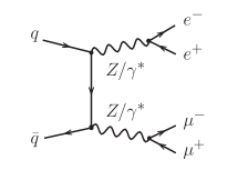
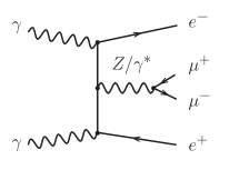
(a)

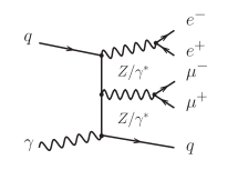
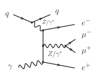
(b)

Figure 1: Example Born-level (a) and real-emissions diagrams (b) contributing to $pp\to e^{+}e^{-}\mu^{+}\mu^{-}+X$ at $\mathcal{O}{\left(\alpha^{4}\right)}$ and $\mathcal{O}{\left(\alpha^{5}\right)}$, respectively.

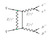
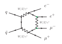
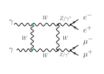
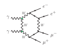
Figure 2: Example one-loop diagrams contributing to $pp\to e^{+}e^{-}\mu^{+}\mu^{-}$ at $\mathcal{O}{\left(\alpha^{5}\right)}$.

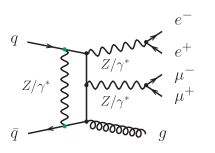
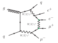
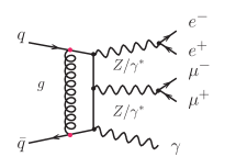
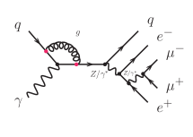
Figure 3: Example one-loop diagrams contributing to $pp\to e^{+}e^{-}\mu^{+}\mu^{-}j$ at $\mathcal{O}{\left(\alpha_{s}\alpha^{5}\right)}$.

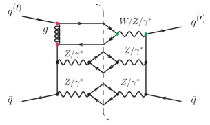
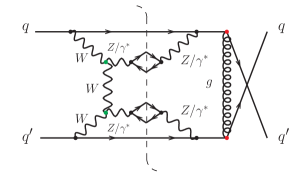
Figure 4: Example real-emission QCD–EW interference contributions in $\displaystyle\bar{q}^{\text{\raisebox{0.75pt}{\scalebox{0.5}{(}}}\hskip 3.7pt\text{\raisebox{0.75pt}{\scalebox{0.5}{)}}}}\displaystyle\bar{q}^{\text{\raisebox{0.75pt}{\scalebox{0.5}{(}}}\hskip 3.7pt\text{\raisebox{0.75pt}{\scalebox{0.5}{)}}}}\to e^{+}e^{-}\mu^{+}\mu^{-}\displaystyle\bar{q}^{\text{\raisebox{0.75pt}{\scalebox{0.5}{(}}}\hskip 3.7pt\text{\raisebox{0.75pt}{\scalebox{0.5}{)}}}}\displaystyle\bar{q}^{\text{\raisebox{0.75pt}{\scalebox{0.5}{(}}}\hskip 3.7pt\text{\raisebox{0.75pt}{\scalebox{0.5}{)}}}}$.

Jet-associated production

The leading-order channels contributing to the associated production of $e^{+}e^{-}\mu^{+}\mu^{-}$ with at least one additional parton which can constitute a jet are given by

$$\begin{split}&q\,\bar{q}\to e^{+}e^{-}\mu^{+}\mu^{-}\,g\quad\text{and}\quad g\,\displaystyle\bar{q}^{\text{\raisebox{0.75pt}{\scalebox{0.5}{(}}}\hskip 3.7pt\text{\raisebox{0.75pt}{\scalebox{0.5}{)}}}}\to e^{+}e^{-}\mu^{+}\mu^{-}\,\displaystyle\bar{q}^{\text{\raisebox{0.75pt}{\scalebox{0.5}{(}}}\hskip 3.7pt\text{\raisebox{0.75pt}{\scalebox{0.5}{)}}}}\quad\text{at}\quad\mathcal{O}{\left(\alpha_{s}\alpha^{4}\right)}\;.\end{split}$$

Corresponding Born-level diagrams can be easily visualised by attaching an additional external gluon to $q\bar{q}$-initiated graphs as the one depicted in Fig. 1(a). The set of partonic channels contributing to the one-jet process at the one-loop level contains

$$\begin{split}&q\,\bar{q}\to e^{+}e^{-}\mu^{+}\mu^{-}\,g\,,\quad g\,\displaystyle\bar{q}^{\text{\raisebox{0.75pt}{\scalebox{0.5}{(}}}\hskip 3.7pt\text{\raisebox{0.75pt}{\scalebox{0.5}{)}}}}\to e^{+}e^{-}\mu^{+}\mu^{-}\,\displaystyle\bar{q}^{\text{\raisebox{0.75pt}{\scalebox{0.5}{(}}}\hskip 3.7pt\text{\raisebox{0.75pt}{\scalebox{0.5}{)}}}}\quad\text{and}\quad\\ &q\,\bar{q}\to e^{+}e^{-}\mu^{+}\mu^{-}\,\gamma\,,\quad\gamma\,\displaystyle\bar{q}^{\text{\raisebox{0.75pt}{\scalebox{0.5}{(}}}\hskip 3.7pt\text{\raisebox{0.75pt}{\scalebox{0.5}{)}}}}\to e^{+}e^{-}\mu^{+}\mu^{-}\,\displaystyle\bar{q}^{\text{\raisebox{0.75pt}{\scalebox{0.5}{(}}}\hskip 3.7pt\text{\raisebox{0.75pt}{\scalebox{0.5}{)}}}}\quad\text{at}\quad\mathcal{O}{\left(\alpha_{s}\alpha^{5}\right)}\;.\end{split}$$

In contrast to the inclusive case, new channels emerge, where the external gluon gets replaced by a photon. So besides the canonical EW loops inserted in the LO channels, also QCD-loop corrections to channels with external photons, contributing at tree-level only in subleading orders, appear. See Fig. 3 for examples of one-loop amplitudes corresponding to the two types of processes. New channels also open for the real corrections:

$$\begin{split}&q\,\bar{q}\to e^{+}e^{-}\mu^{+}\mu^{-}\,g\,\gamma\,,\quad g\,\displaystyle\bar{q}^{\text{\raisebox{0.75pt}{\scalebox{0.5}{(}}}\hskip 3.7pt\text{\raisebox{0.75pt}{\scalebox{0.5}{)}}}}\to e^{+}e^{-}\mu^{+}\mu^{-}\,\gamma\,\displaystyle\bar{q}^{\text{\raisebox{0.75pt}{\scalebox{0.5}{(}}}\hskip 3.7pt\text{\raisebox{0.75pt}{\scalebox{0.5}{)}}}}\,,\quad\\ &\gamma\,\displaystyle\bar{q}^{\text{\raisebox{0.75pt}{\scalebox{0.5}{(}}}\hskip 3.7pt\text{\raisebox{0.75pt}{\scalebox{0.5}{)}}}}\to e^{+}e^{-}\mu^{+}\mu^{-}\,g\,\displaystyle\bar{q}^{\text{\raisebox{0.75pt}{\scalebox{0.5}{(}}}\hskip 3.7pt\text{\raisebox{0.75pt}{\scalebox{0.5}{)}}}}\,,\quad\gamma\,g\to e^{+}e^{-}\mu^{+}\mu^{-}\,q\,\bar{q}\quad\text{and}\quad\displaystyle\bar{q}^{\text{\raisebox{0.75pt}{\scalebox{0.5}{(}}}\hskip 3.7pt\text{\raisebox{0.75pt}{\scalebox{0.5}{)}}}}\,\displaystyle\bar{q}^{\text{\raisebox{0.75pt}{\scalebox{0.5}{(}}}\hskip 3.7pt\text{\raisebox{0.75pt}{\scalebox{0.5}{)}}}}\to e^{+}e^{-}\mu^{+}\mu^{-}\,\displaystyle\bar{q}^{\text{\raisebox{0.75pt}{\scalebox{0.5}{(}}}\hskip 3.7pt\text{\raisebox{0.75pt}{\scalebox{0.5}{)}}}}\,\displaystyle\bar{q}^{\text{\raisebox{0.75pt}{\scalebox{0.5}{(}}}\hskip 3.7pt\text{\raisebox{0.75pt}{\scalebox{0.5}{)}}}}\quad\text{at}\quad\mathcal{O}{\left(\alpha_{s}\alpha^{5}\right)}\;.\end{split}$$

The last process, involving four external quarks and no external photon, deserves an explicit discussion. This contribution is completely infrared finite and, thus, separable from the other processes. It consists of an interference of diagrams of $\mathcal{O}{\left(g_{s}^{2}e^{4}\right)}$ and $\mathcal{O}{\left(e^{6}\right)}$, commonly referred to as QCD production and EW production, respectively. Due to the colour algebra involved they typically entail $s$-/$t$-channel or $t$-/$u$-channel interferences. Two examples are given in Fig. 4. It is noteworthy that, due to their nature as interference terms, they are of indeterminate sign, and are typically small for inclusive observables. However, as they are the only contributions at this order which can contain two valence quarks as initial states, e.g. $uu$, $ud$, or $dd$, they can still be quite sizeable in the TeV range.

Loop-induced production

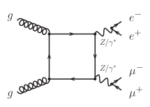
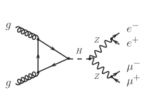
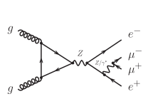
(a)

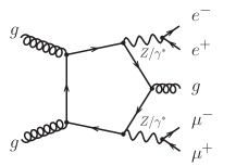
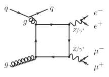
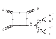
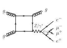
(b)

Figure 5: Example loop-squared contributions to $pp\to e^{+}e^{-}\mu^{+}\mu^{-}$ (a) and $pp\to e^{+}e^{-}\mu^{+}\mu^{-}j$ (b).

Although technically only a NNLO correction, gluon-induced loop-squared contributions have a numerically important phenomenological impact, both for inclusive and one-jet observables. Therefore, in addition to the standard quark-induced four-lepton production processes, we consider the gluon-induced loop-squared contributions as one component of our multijet-merging approach. Here, immediately the question of systematically separating both production modes arises, as they coexist at higher orders that are at least approximated in any calculation matched to a parton shower. To this end, keeping in mind the parton shower’s generating functional of Eq. (3.3) and following [104], we include all diagrams where all four leptons couple through one (or more) electroweak gauge boson to the closed quark loop, but not any other quarks in the process. This excludes in particular diagrams where one lepton pair is radiated off an external quark. This means, that while

$$g\,g\to e^{+}e^{-}\mu^{+}\mu^{-}\quad\text{at}\quad\mathcal{O}{\left(\alpha_{s}^{2}\alpha^{4}\right)}$$

solely constitutes inclusive loop-induced four-lepton production,

$$g\,g\to e^{+}e^{-}\mu^{+}\mu^{-}\,g\,,\quad g\,\displaystyle\bar{q}^{\text{\raisebox{0.75pt}{\scalebox{0.5}{(}}}\hskip 3.7pt\text{\raisebox{0.75pt}{\scalebox{0.5}{)}}}}\to e^{+}e^{-}\mu^{+}\mu^{-}\,\displaystyle\bar{q}^{\text{\raisebox{0.75pt}{\scalebox{0.5}{(}}}\hskip 3.7pt\text{\raisebox{0.75pt}{\scalebox{0.5}{)}}}}\quad\text{and}\quad q\,\bar{q}\to e^{+}e^{-}\mu^{+}\mu^{-}\,g\quad\text{at}\quad\mathcal{O}{\left(\alpha_{s}^{3}\alpha^{4}\right)}$$

contribute for the jet-associated final state. Fig. 5 contains example Feynman diagrams contributing to the loop-induced modes of hadronic $e^{+}e^{-}\mu^{+}\mu^{-}$ (a) and $e^{+}e^{-}\mu^{+}\mu^{-}j$ (b) production. This comprises triangle-, box- and pentagon-type contributions. We include light quarks and top quarks in the closed fermion loops and allow for both double- and single-resonant as well as Higgs-boson mediated topologies. It is important to note, that in the single-resonant diagrams the $Z$-boson couples through its axial component in triangle-like and its vector component in box-like topologies.

Electroweak corrections to these loop-induced processes are of two-loop complexity, they have not been calculated yet, and consequently we do not consider them in this paper.

4.2 Numerical inputs and event-selection cuts

All calculations shown in this work are performed in the Sherpa+O PEN L OOPS /Recola [37, 36, 8, 109, 9, 110] framework, allowing for a fully automated calculation of cross sections and observables at next-to-leading order in the strong and electroweak sector of the Standard Model. In this framework, renormalised QCD and EW virtual corrections are provided by O PEN L OOPS [8, 109] and Recola [9] for the standard $4\ell$ and $4\ell+j$ and all loop-induced processes. Both programs use the Collier tensor-reduction library [111]. In addition, O PEN L OOPS also uses CutTools [112] together with O NE L OOP [113]. All remaining tasks, i.e. the tree-level Born and real-emission matrix elements as well as the bookkeeping of partonic subprocesses, phase-space integration, and the subtraction of all QCD and QED infrared singularities, are performed by Sherpa using the A MEGIC and C OMIX matrix-element generators [114, 115, 18, 15]. Sherpa in combination with O PEN L OOPS and/or Recola has been employed successfully in a range of different calculations at NLO EW [19, 46, 53, 110, 94, 22, 23, 103, 24, 30, 106, 108] and has been validated against other tools in [116]. For off-shell inclusive $ZZ$ production in particular, we have recomputed the results of [51, 52, 108] and excellent agreement was found. The analyses for the following results have been implemented in Rivet [117, 118].

We present predictions for proton–proton collisions at $\sqrt{s}=13\,\text{TeV}$. For the masses and widths we use the following values [119, 120]

$M_{W}^{\text{OS}}$	​​=​​	80.385 GeV	$\Gamma_{W}^{\text{OS}}$	​​=​​	2.085 GeV
$M_{Z}^{\text{OS}}$	​​=​​	91.1876 GeV	$\Gamma_{Z}^{\text{OS}}$	​​=​​	2.4952 GeV
$M_{h}$	​​=​​	125.0 GeV	$\Gamma_{h}$	​​=​​	0.00407 GeV
$m_{t}$	​​=​​	173.2 GeV	$\Gamma_{t}$	​​=​​	0 .

All other particles are treated as massless, in particular we are working in the five-flavour scheme. Note, we throughout assume the CKM quark-mixing matrix to be diagonal. The pole masses and widths used in the computation are obtained from the given on-shell (OS) values for the $W$ and $Z$ bosons according to [121]

$$M_{\text{V}}=\frac{M_{\text{V}}^{\text{OS}}}{\sqrt{1+(\Gamma_{\text{V}}^{\text{OS}}/M_{\text{V}}^{\text{OS}})^{2}}}\;,\qquad\Gamma_{\text{V}}=\frac{\Gamma_{\text{V}}^{\text{OS}}}{\sqrt{1+(\Gamma_{\text{V}}^{\text{OS}}/M_{\text{V}}^{\text{OS}})^{2}}}\;,$$ (4.1)

with ${\text{V}}=W,Z$. We work in the complex-mass scheme [122, 123], where the complex masses and the weak mixing angle are given by

$$\mu_{i}^{2}=M_{i}^{2}-\mathrm{i}M_{i}\Gamma_{i}\qquad\text{and}\qquad\sin^{2}\theta_{w}=1-\frac{\mu_{W}^{2}}{\mu_{Z}^{2}}\;.$$ (4.2)

Per default we use the $G_{\mu}$ input parameter and renormalisation scheme [124, 125] with

$$G_{\mu}=1.16637\times 10^{-5}\,\text{GeV}^{-2}\qquad\text{and}\qquad\alpha_{G_{\mu}}=\frac{\sqrt{2}}{\pi}\,G_{\mu}M_{W}^{2}\left(1-\frac{M_{W}^{2}}{M_{Z}^{2}}\right)\;.$$ (4.3)

In order to gauge the impact of the choice for the EW renormalisation scheme, we also consider results obtained in the $\alpha(M_{Z}^{2})$ scheme, with

$$\alpha(M_{Z}^{2})=1/128.802$$ (4.4)

as an input parameter, and renormalise the amplitudes accordingly. All other parameters remain unchanged. The difference between these two choices can be seen as a (partial) missing-higher-order uncertainty. See Refs. [2, 126, 127] for recent discussions of EW input parameter and renormalisation schemes.

As parton distribution function (PDF) we use the NNPDF31_nlo_as_0118_luxqed set [128], interfaced through Lhapdf [129]. The extraction of the photon content is based on [130]. The value of the strong coupling is chosen accordingly, i.e.

$$\alpha_{\text{s}}(M^{2}_{Z})=0.118\;.$$ (4.5)

For the event selection, we first combine the charged leptons with collinear photons within a standard cone of radius $R=0.1$. The so dressed leptons $\ell$ are then required to pass the following selection cuts for their transverse momentum, rapidity and distance to other dressed leptons $\ell^{\prime}$:

$$p_{\mathrm{T},\ell}>20\,\text{GeV},\qquad\qquad|y_{\ell}|<2.5,\qquad\qquad\Delta R_{\ell\ell^{\prime}}>0.1\,.$$ (4.6)

These criteria define the fiducial phase space of our analysis for inclusive setups, such as the $e^{+}e^{-}\mu^{+}\mu^{-}$ fixed-order calculation or the multijet-merged one.

For the fixed-order evaluation of $e^{+}e^{-}\mu^{+}\mu^{-}j$, as well as in the analysis of jet observables for the multijet-merging samples, the additional jet(s) $j$ are defined with the anti-$k_{t}$ algorithm [131] with $R=0.4$ and

$$p_{\mathrm{T},j}>30\,\text{GeV},\qquad\qquad|y_{j}|<4.5,\qquad\qquad\Delta R_{\ell j}>0.4\,.$$ (4.7)

All particles that are not part of the previously defined dressed leptons are considered as input to the jet algorithm.

4.3 Fixed-order results

In this section we validate the approximations introduced in Sec. 3.2 applied to $pp\to e^{+}e^{-}\mu^{+}\mu^{-}$ and $pp\to e^{+}e^{-}\mu^{+}\mu^{-}j$ at LO against the respective full NLO EW results. The $\text{EW}_{\text{virt}}$ and $\text{EW}_{\text{sud}}$ computations include YFS soft-photon resummation as discussed in Sec. 3.2, in order to account for real-emission kinematics and effects. We further provide predictions based on matching the full NLO EW result with NLL EW Sudakov resummation, as an improved description including the all-orders resummed EW corrections in the region where they are large.

For these calculations, the renormalisation and factorisation scales are set in accordance with Refs. [132, 106], i.e.

$$\mu_{\mathrm{R}}=\mu_{\mathrm{F}}=\tfrac{1}{2}\left(E_{\mathrm{T},ee}+E_{\mathrm{T},\mu\mu}\right)\,,$$

with the transverse energies of the two vector bosons given by

$$E_{\text{T},\ell\ell}=\sqrt{m_{\ell\ell}^{2}+p^{2}_{\mathrm{T},\ell\ell}}\,.$$

Here, $m_{\ell\ell}$ and $p_{\mathrm{T},\ell\ell}$ denote the invariant mass and the transverse momentum of the off-shell charged dressed lepton pair.

Further, all inclusive cross sections are given both in the $G_{\mu}$ scheme and in the $\alpha(M_{Z}^{2})$ scheme, with the former being our default choice for the final predictions presented in Sec. 4.4. In addition to the inclusive phase space, we also consider dedicated additional selections focusing on the EW Sudakov region where our matched result formally improves on the pure NLO EW one, and both approximations are in their respective regime of validity. Here, we give the $G_{\mu}$ scheme results only, because we are interested on the effects of the resummation in this region. Finally, we provide differential distributions, including the full NLO EW results in the $G_{\mu}$ and $\alpha(M_{Z}^{2})$ scheme in order to discuss their input-parameter and renormalisation scheme dependence.

Inclusive $e^{+}e^{-}\mu^{+}\mu^{-}$ production

We start by discussing the process $pp\to e^{+}e^{-}\mu^{+}\mu^{-}+X$, for which QCD and EW corrections are known to NNLO and NLO, respectively [47, 48, 49, 50, 51, 52, 53, 54, 55]. We use this setup as an initial benchmark for the approximations described in Sec. 3.2. We report results for the inclusive fiducial cross section in the various calculational schemes in Tab. 1. All approximate treatments for EW corrections as well as the inclusion of the full set of NLO EW corrections reduce the cross section.

Examining the cross sections and higher-order EW corrections summarised in Tab. 1, the different impact of the change of input-parameter and renormalisation scheme on the LO and NLO EW results is the most striking observation. At the leading order, i.e. ${\cal{O}}(\alpha^{4})$, the change of EW scheme amounts to a simple rescaling of the parameter $\alpha$ used in the calculation, as this has different values in the schemes. The values of all masses, widths, and $\sin\theta_{w}$ remain unchanged. In particular, here this change of scheme amounts to an $11.3\text{\,}\mathrm{\char 37\relax}$ difference in the inclusive cross section at LO. At NLO, the scheme dependence is not quite so straight-forward. While the one-loop, mass factorisation and real-emission contributions are again simply rescaled, the scheme-dependent renormalisation contributions differ significantly in magnitude and structure. The result is the expected much smaller, and now oppositely signed, scheme dependence of $-3.8\text{\,}\mathrm{\char 37\relax}$. The relative NLO corrections of $-6.8\text{\,}\%$ and $-19.4\text{\,}\%$ in the $G_{\mu}$ and $\alpha(M_{Z}^{2})$ schemes, respectively, also demonstrate the superior adequacy of the $G_{\mu}$ scheme, caused by its effective partial accounting for the leading universal renormalisation effects originating from the $\rho$-parameter. While this behaviour is well reproduced by the $\text{EW}_{\text{virt}}$ approximation due to its inclusion of the renormalisation terms, the $\text{EW}_{\text{sud}}$ approximation follows the LO behaviour in its scheme dependence. Apart from the parameter renormalisation (PR) logarithms [41, 42] which are however generally not the dominant terms, $\text{EW}_{\text{sud}}$ features no additional scheme-dependence compensation. Finally, the NLO EW${}+{}$NLL $\text{EW}_{\text{sud}}^{\text{exp}}$ prediction largely coincides with the scheme dependence of the NLO EW calculation as the influence of the resummed EW Sudakov exponent is minimal in the inclusive phase space.

Considering only the $G_{\mu}$ scheme, the relative NLO EW corrections are well reproduced, within about $1\text{\,}\%$, by both the $\text{EW}_{\text{virt}}$  and $\text{EW}_{\text{sud}}$ approximations when complemented with the soft-photon resummation. This is because the total correction in this process is driven in roughly equal parts by negative one-loop corrections and the negative impact of energy-loss due to real-photon radiation. The latter process is only described at $\mathcal{O}{\left(\alpha\right)}$ accuracy while the resummation includes the impact of higher-order emissions further reducing the cross section. We have checked that truncating the resummation to $\mathcal{O}{\left(\alpha\right)}$ – i.e. allow at most a single photon to be emitted and expand the form-factor accordingly – results in a much closer reproduction of the exact result. However, given that the $\text{EW}_{\text{virt}}$ and $\text{EW}_{\text{sud}}$ approximations are tailored to the high-energy regime only, their close reproduction of inclusive observables is to some degree accidental. Finally, the relative correction of the NLO EW${}+{}$NLL $\text{EW}_{\text{sud}}^{\text{exp}}$ matched result follows the NLO EW one closely as Sudakov logarithms are small and their resummation does not lead to noticeable effects.

$pp\to e^{+}e^{-}\mu^{+}\mu^{-}$		fiducial cross section	corrections to LO
Scheme	Region	LO	NLO EW	$\text{LO}+\text{EW}_{\text{virt}}{}+\text{YFS}$	$\text{LO}+\text{EW}_{\text{sud}}{}+\text{YFS}$	$\text{LO}+\text{EW}_{\text{sud}}^{\text{exp}}{}+\text{YFS}$	NLO EW${}+{}$NLL $\text{EW}_{\text{sud}}^{\text{exp}}$
$G_{\mu}$	inclusive	9.819 fb	$-6.8$ %	$-7.9$ %	$-7.3$ %	$-7.2$ %	$-6.7$ %
$\alpha(M_{Z}^{2})$		10.928 fb	$-19.4$ %	$-20.2$ %	$-7.7$ %	$-7.6$ %	$-19.3$ %
$\delta^{\alpha(M_{Z}^{2})}_{G_{\mu}}$		11.3 %	$-3.8$ %	$-3.6$ %	$10.8$ %	$10.8$ %	$-3.7$ %
$G_{\mu}$	high energy	$4.27\cdot 10^{-3}$ fb	$-42$ %	$-45$ %	$-39$ %	$-33$ %	$-36$ %

Table 1: Inclusive fiducial cross sections for $pp\to e^{+}e^{-}\mu^{+}\mu^{-}$ at $\sqrt{s}=13\,\,\text{TeV}$ at LO for the $G_{\mu}$ and the $\alpha(M_{Z}^{2})$ scheme, along with the relative corrections for NLO EW, NLO EW${}+{}$NLL $\text{EW}_{\text{sud}}^{\text{exp}}$ and the $\text{EW}_{\text{sud}}$ and $\text{EW}_{\text{virt}}$ approximations. The table also gives the relative differences $\delta^{\alpha(M_{Z}^{2})}_{G_{\mu}}$ of the $\alpha(M_{Z}^{2})$ scheme with respect to the default $G_{\mu}$ scheme, and results for the “high-energy” region, which requires $p_{\text{T},2e}>$600\text{\,}\mathrm{GeV}$$ in addition to the fiducial cuts.

Tab. 1 accompanies the inclusive cross section with a “high energy” region requiring additionally $p_{\text{T},2e}>$600\text{\,}\mathrm{GeV}$$, thus entering the region where the Sudakov logarithms become sizeable and dominate the total NLO EW corrections. As expected, the resummation of the Sudakov logarithms is important here, giving a $6\text{\,}\mathrm{\char 37\relax}$ smaller correction with respect to LO in the NLO EW${}+{}$NLL $\text{EW}_{\text{sud}}^{\text{exp}}$ calculation as compared to the NLO EW result (or a $10\text{\,}\mathrm{\char 37\relax}$ increase of the cross section relative to it).

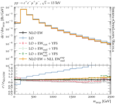
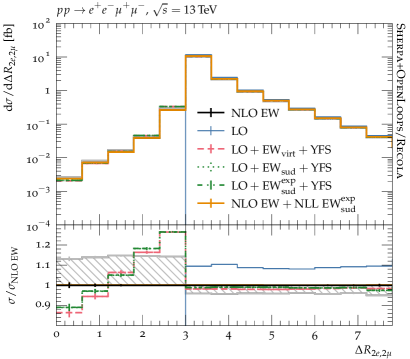
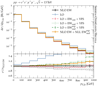
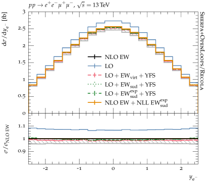
Figure 6: Observable distributions for the $pp\to e^{+}e^{-}\mu^{+}\mu^{-}$ process. From top left to bottom right we show: the four-lepton invariant mass $m_{2e2\mu}$, the $Z$-boson distance $\Delta R_{2e,2\mu}$, the transverse momentum of the di-electron pair $p_{\text{T},2e}$, and the rapidity of the electron $y_{\text{e}^{-}}$. Results are given at LO and NLO EW and compared to approximative EW calculations. The NLO EW is given for the $G_{\mu}$ (black line) and $\alpha(M_{Z}^{2})$ (grey line) renormalisation schemes, and the span between the two is marked by a hatched band. All predictions are calculated using Sherpa+O PEN L OOPS /Recola.

We show differential distributions obtained in the various calculational schemes in Fig. 6, where in addition to the nominal predictions we indicate the NLO EW scheme dependence with a grey hatched band. The observables considered are the invariant mass of the four-lepton system $m_{2e2\mu}$, the $Z$-boson distance $\Delta R_{2e,2\mu}$, the transverse momentum of the di-electron pair $p_{\text{T},2e}$, and the electron rapidity $y_{\text{e}^{-}}$.

We start by noticing that the overall good agreement between the $\text{EW}_{\text{virt}}$ approximation and the full NLO EW observed for the total cross section is also found for all the distributions. The only significant difference comes from phase-space regions dominated by real-photon radiation, such as $\Delta R_{2e,2\mu}<\pi$. There one can see the impact of resumming soft photons through YFS versus treating them at fixed order, which exhibits the main advantage of including YFS resummation. We have indeed checked that if we expand the YFS resummation to $\mathcal{O}{\left(\alpha\right)}$, as discussed above, we reproduce the NLO EW result throughout, as a result of the inclusion on exact NLO QED corrections in the YFS resummation. A similar overall good agreement can be seen in the Sudakov approximation.

To further discuss the impact and the effects of the EW approximations we need to distinguish between energy-dependent observables, such as the invariant mass of the four leptons and the $p_{\mathrm{T}}$ of the electron pair, and energy-independent observables, such as the separation of the two lepton pairs and the rapidity of the electron. The former class shows, as expected, a suppression in the high-energy tail of distributions that feature a similar shape for both observables. The size of the suppression is, however, different, but we find that overall the various approximations are all within $5$–$10\text{\,}\mathrm{\char 37\relax}$ of the exact NLO EW result. The matched NLO EW${}+{}$NLL $\text{EW}_{\text{sud}}^{\text{exp}}$ result, shown here for the first time, has the expected behaviour, interpolating from the NLO EW result at low energies to the exponentiated Sudakov logarithms at high energies. In particular, we notice that at high energies the resummation leads to a reduction of the suppression of about $5$–$10\text{\,}\mathrm{\char 37\relax}$ compared to the fixed-order Sudakov approximation. The latter class of observables, on the other hand, has no energy dependence, and encapsulates the $k$-factors of the total cross-section table uniformly distributed across the available phase space. The only deviation from this, as discussed above, is the region sensitive to additional real radiation, e.g. $\Delta R_{2e,2\mu}<\pi$ or $m_{2e2\mu}<2M_{Z}$.

Jet-associated production

We now turn our attention to the production of two lepton pairs associated by an $R=0.4$ anti-$k_{t}$ jet with $p_{\mathrm{T},j}>30\,\text{GeV}$, see Sec. 4.2. To the best of our knowledge, this is the first time that NLO EW corrections are shown for this specific process, though the technology is readily available. Nevertheless, the comparison between the full NLO EW and the various approximations requires more care, as the full NLO EW result contains QCD corrections to lower-order Born terms as well as QCD–EW interference contributions, see Figs. 3 and 4 respectively, which are not captured by either approximation. However, as stressed before, such interference contributions are typically small for inclusive observables. Nonetheless, with the QCD–EW interference terms in particular being the only contributions at this order which can contain two valence quarks as initial state, e.g. $uu$, $du$, or $dd$, they can be quite sizeable in the TeV range and potentially spoil the quality of the $\text{EW}_{\text{sud}}$ and $\text{EW}_{\text{virt}}$ approximations.

$pp\to e^{+}e^{-}\mu^{+}\mu^{-}j$		fiducial cross section	corrections to LO
Scheme	Region	LO	NLO EW	$\text{LO}+\text{EW}_{\text{virt}}{}+\text{YFS}$	$\text{LO}+\text{EW}_{\text{sud}}{}+\text{YFS}$	$\text{LO}+\text{EW}_{\text{sud}}^{\text{exp}}{}+\text{YFS}$	NLO EW${}+{}$NLL $\text{EW}_{\text{sud}}^{\text{exp}}$
$G_{\mu}$	inclusive	5.170 fb	$-6.6$ %	$-8.5$ %	$-6.9$ %	$-6.7$ %	$-6.4$ %
$\alpha(M_{Z}^{2})$		5.754 fb	$-19.2$ %	$-20.6$ %	$-6.9$ %	$-6.7$ %	$-19.0$ %
$\delta^{\alpha(M_{Z}^{2})}_{G_{\mu}}$		11.29 %	$-3.7$ %	$-3.4$ %	$11.3$ %	$11.3$ %	$-3.7$ %
$G_{\mu}$	high energy	$6.64\cdot 10^{-3}$ fb	$-33$ %	$-37$ %	$-30$ %	$-25$ %	$-29$ %

Table 2: Inclusive fiducial cross sections for $pp\to e^{+}e^{-}\mu^{+}\mu^{-}j$ at $\sqrt{s}=13\,\,\text{TeV}$ at LO for the $G_{\mu}$ and the $\alpha(M_{Z}^{2})$ scheme, along with the relative corrections for NLO EW, NLO EW${}+{}$NLL $\text{EW}_{\text{sud}}^{\text{exp}}$ and the $\text{EW}_{\text{sud}}$ and $\text{EW}_{\text{virt}}$ approximations. The table also gives the relative differences $\delta^{\alpha(M_{Z}^{2})}_{G_{\mu}}$ of the $\alpha(M_{Z}^{2})$ scheme with respect to the default $G_{\mu}$ scheme, and results for the “high-energy” region, which requires $p_{\text{T},2e}>$600\text{\,}\mathrm{GeV}$$ in addition to the fiducial cuts.

The discussion for this process follows closely that for the four-lepton final state. In Tab. 2 we report results for the inclusive fiducial cross sections at LO, NLO EW, LO+$\text{EW}_{\text{virt}}$+YFS, LO+$\text{EW}_{\text{sud}}$+YFS, LO+$\text{EW}_{\text{sud}}^{\text{exp}}$+YFS, and NLO EW${}+{}$NLL $\text{EW}_{\text{sud}}^{\text{exp}}$, once again, both for the $G_{\mu}$ and the $\alpha(M_{Z}^{2})$ scheme, and similar conclusions can be drawn here. Notably, the size of the NLO EW corrections with respect to the LO are only slightly reduced, which confirms the known behaviour that EW corrections with extra QCD jets are roughly of the same size. In particular we find that they are about $-6.6\text{\,}\mathrm{\char 37\relax}$ and $-19.2\text{\,}\mathrm{\char 37\relax}$ with respect to the LO result for the $G_{\mu}$ and the $\alpha(M_{Z}^{2})$ schemes, respectively. In addition, we find a slightly reduced agreement between the NLO EW and the $\text{EW}_{\text{virt}}$ approximation, amounting to roughly $-2\text{\,}\mathrm{\char 37\relax}$ with respect to the NLO EW result for both the $G_{\mu}$ and the $\alpha(M_{Z}^{2})$ scheme. While numerically small, this may be attributed to the fact that, while the QCD corrections to lower-order Born contributions are included, the additional four-quark channels discussed are not present in the $\text{EW}_{\text{virt}}$ approximation. Here, the $\text{EW}_{\text{sud}}$ approximation shows a better level of agreement, despite more contributions get discarded in this approximation. Hence, the quality of reproduction of the exact result is to some degree accidental for both approximations, as they are tailored to account for the high-energy regime in particular. Nonetheless, it is reassuring that, at least in the $G_{\mu}$ scheme, both reproduce the exact result qualitatively quite well. In similar fashion, the resummed Sudakov approximation changes the fixed-order result very little, both in the pure Sudakov approximation and the matched NLO EW${}+{}$NLL $\text{EW}_{\text{sud}}^{\text{exp}}$ calculation.

In Fig. 7 we now show the same four observables as for the 0-jet case. In comparison, we find a small reduction of the EW scheme dependence, slightly reduced NLO EW corrections, and a very similar behaviour of the approximation with respect to the NLO EW results. This suggests a factorisation of the logarithmic corrections of the $\text{EW}_{\text{virt}}$ and $\text{EW}_{\text{sud}}$ approximation with respect to additional QCD emissions. This can be related to the fact that the sum of EW charges of the external lines remains unaffected by QCD corrections [106].

Due to the presence of the jet, the $\Delta R_{2e,2\mu}<\pi$ region is now already populated at LO. This results in a good agreement between the NLO EW calculation and the approximations also in this region, removing the discontinuity seen in the inclusive $ZZ$ results. This is also true for the scheme dependence of the NLO EW calculation, since now the entire observable range receives NLO contributions. In fact, we observe a nearly constant NLO correction of about $5$–$10\text{\,}\mathrm{\char 37\relax}$.

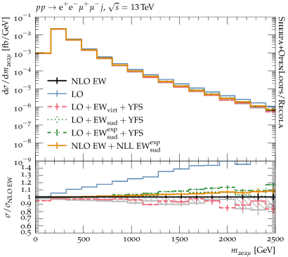
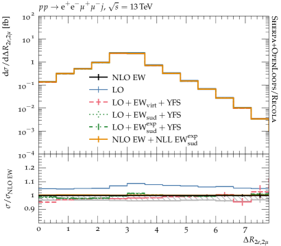
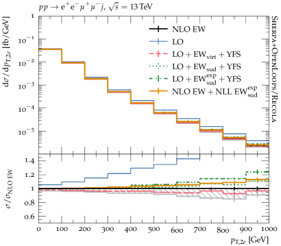
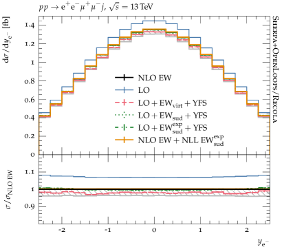
Figure 7: Leptonic observable distributions as shown in Fig. 6 but for the $pp\to e^{+}e^{-}\mu^{+}\mu^{-}j$ process.

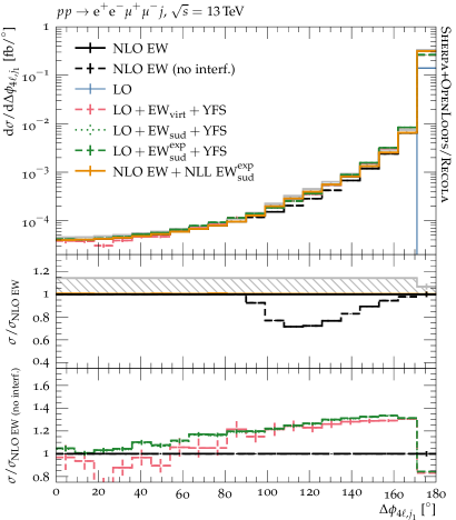
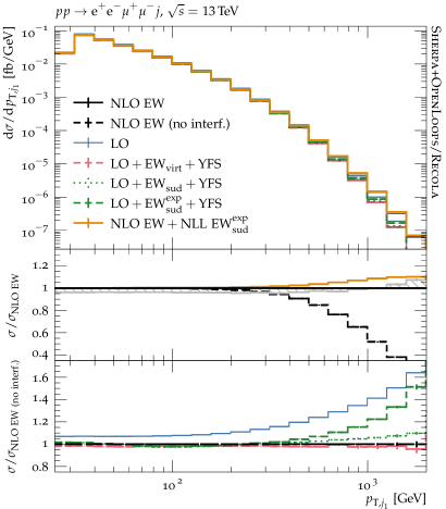
Figure 8: Distributions for the azimuthal distance between the four-lepton system and the leading jet $\Delta\phi_{4\ell,j_{1}}$ (left), and the leading-jet transverse momentum $p_{\mathrm{T},j_{1}}$ (right) for the $pp\to e^{+}e^{-}\mu^{+}\mu^{-}j$ process. They are given at LO and at NLO EW and compared to approximative EW calculations. The NLO EW is given for the $G_{\mu}$ (black line) and $\alpha(M_{Z}^{2})$ (grey line) renormalisation schemes, and the span between the two is marked by a hatched band. In addition, the NLO EW is plotted without interference terms (“no interf.”). All predictions are calculated using Sherpa+O PEN L OOPS /Recola.

In Fig. 8 we additionally present two observables for the leading (i.e. highest-$p_{T}$) jet: the angular separation between it and the four-lepton system $\Delta\phi_{4\ell,j_{1}}$, and its transverse-momentum $p_{\text{T},j_{1}}$. For these observables we display an additional result, labelled as “NLO EW (no interf.)”. This line represents the NLO EW result for the $G_{\mu}$ scheme excluding the finite real correction coming from the interference of diagrams of orders $\mathcal{O}(g_{s}^{2}g^{4})$ and $\mathcal{O}(g^{6})$ for $pp\to e^{+}e^{-}\mu^{+}\mu^{-}jj$. Note that this contribution is by construction not included in either the EW approximations or the YFS approach, since it is a finite real-emission correction.

For the angular separation $\Delta\phi_{4\ell,j_{1}}$, Born kinematics produce back-to-back configurations only, i.e. $\Delta\phi_{4\ell,j_{1}}=$180\text{\,}\mathrm{\SIUnitSymbolDegree}$$. Hence, for the two approximations the $\Delta\phi_{4\ell,j_{1}}<$180\text{\,}\mathrm{\SIUnitSymbolDegree}$$ region is only populated via YFS photon emissions. We find that the shape of the NLO EW distribution is reproduced well by YFS, although there is a shape difference for intermediate angles $$90\text{\,}\mathrm{\SIUnitSymbolDegree}$<\Delta\phi_{4\ell,j_{1}}<$180\text{\,}\mathrm{\SIUnitSymbolDegree}$$. Comparing the full NLO EW with the “NLO EW (no interf.)” result we conclude that this difference is entirely due to these interference terms, which are missing from the LO+YFS simulation. The resulting difference in rate is $30\text{\,}\%$ at large $\Delta\phi_{4\ell,j_{1}}$ and decreases towards zero with decreasing $\Delta\phi_{4\ell,j_{1}}$.

For the same reason we find a strong discrepancy between the NLO EW calculation and the approximations for $p_{\text{T},j_{1}}>$300\text{\,}\mathrm{GeV}$$. Again this is entirely due to the presence of the interference terms, and once they are removed we find very good agreement. In particular, we then observe an excellent agreement with the $\text{EW}_{\text{virt}}$ approximation, and a good agreement with the $\text{EW}_{\text{sud}}$ one.

With these observations we infer that adding a jet veto in order to limit the activity of the finite contribution would allow the approximations introduced here to be even closer to the full NLO EW results, see [106], where this is studied for $\text{EW}_{\text{virt}}$ in the context of $WW$ and $WWj$ production. Note that adding a jet veto introduces further logarithms related to the jet-veto scale which would in general need to be resummed. Please also note, that even in the absence of jet vetoes, the picture changes once QCD corrections, which are of the order of $100\text{\,}\%$ in this regime [133], are included, rendering the impact of the QCD–EW interference contributions less marked.

4.4 Multijet-merged results

In this section we use the approximations validated for both $ZZ$ and $ZZj$ production in Sec. 4.3 to incorporate higher-order electoroweak effects in a particle-level calculation, as introduced in Sec. 3. Before we present our final results, however, we are first proceeding with a structural analysis and validation of our calculation in order to understand the interplay of each contribution of the multijet-merged computation and their impact on the final result.

Structural analysis and validation

The MePs@Nlo predictions are obtained by merging NLO QCD matrix elements for $pp\to e^{+}e^{-}\mu^{+}\mu^{-}$ and $pp\to e^{+}e^{-}\mu^{+}\mu^{-}j$ and the QCD tree-level matrix elements for $pp\to e^{+}e^{-}\mu^{+}\mu^{-}jj$ and $pp\to e^{+}e^{-}\mu^{+}\mu^{-}jjj$. As a way to study the interplay between QCD and EW corrections, we also provide results at MePs@Lo accuracy, which we obtain by merging the same parton multiplicities $n=0,1,2,3$, but in this case all are evaluated at LO only, i.e. $\mathcal{O}{\left(\alpha_{s}^{n}\alpha^{4}\right)}$. The merging is performed using the algorithms outlined in Sec. 3.1, with the merging scale set to

$$Q_{\text{cut}}=30\;\,\text{GeV}\,.$$ (4.8)

The renormalisation, factorisation, and resummation scales are set according to the CKKW scale-setting prescription. The renormalisation scale is thereby defined through $\mu_{\mathrm{R}}=\mu_{\text{CKKW}}$ [134], with

$$\begin{split}\alpha_{s}^{n}(\mu_{\text{CKKW}}^{2})=&\;\alpha_{s}(t_{1})\cdots\alpha_{s}(t_{n})\;,\end{split}$$ (4.9)

where the $t_{i}$ are the reconstructed shower-emission scales of the $n$-jet hard-process configuration. The scale of the inner core process, $\mu_{\text{core}}$, is set to

$$\mu_{\text{core}}=\tfrac{1}{2}\,\left(E_{\mathrm{T},ee}+E_{\mathrm{T},\mu\mu}\right)\;,$$ (4.10)

and is used to define the factorisation and resummation scales via $\mu_{\mathrm{F}}=\mu_{\mathrm{Q}}=\mu_{\text{core}}$. Lastly, note that the simulation of soft and collinear photon emissions off the final-state leptons in the YFS formalism is enabled for all results in this section.

We use the QCD MePs@Nlo prediction as a reference to determine the impact of approximate EW corrections. We incorporate EW correction in the $\text{EW}_{\text{virt}}$ approximation into the underlying MePs@Nlo calculation, both in the additive and the multiplicative scheme, as defined in Eq. (3.13) and Eq. (3.11), respectively. Furthermore, we consider the $\text{EW}_{\text{sud}}$ approximation as an alternative.

Finally, we give the QCD MePs@Lo prediction, both as-is, serving as an additional reference for the inclusive fiducial cross section, and including $\text{EW}_{\text{sud}}$ corrections. To better capture non-trivial kinematical effects, we multiply this LO accurate prediction by the global QCD $k$-factor given by the ratio of the inclusive fiducial cross sections of the MePs@Nlo and MePs@Lo calculations. Note that $\text{EW}_{\text{virt}}$ is not readily available for this MePs@Lo calculation, given that it requires NLO EW one-loop matrix elements for all multiplicities (i.e. up to $n=3$), and a local $k$-factor mechanism as described for MePs@Nlo in Eq. (3.12) to make up for missing one-loop matrix elements is not yet implemented for MePs@Lo in Sherpa.

$pp\to e^{+}e^{-}\mu^{+}\mu^{-}+\text{jets}$		fiducial cross section		corrections to $\text{{MePs@Nlo}}+\text{YFS}$
Scheme	Region	$\text{{MePs@Lo}}+\text{YFS}$	$\text{{MePs@Nlo}}+\text{YFS}$	$\times\,\text{EW}_{\text{virt}}{}$	$\times\,\text{EW}_{\text{sud}}{}$	$\times\,\text{EW}_{\text{sud}}^{\text{exp}}{}$
$G_{\mu}$	inclusive	11.10 fb	13.34 fb	$-4$ %	$-4$ %	$-3$ %

Table 3: Inclusive fiducial cross sections for $pp\to e^{+}e^{-}\mu^{+}\mu^{-}$ + jets at $\sqrt{s}=$13\text{\,}\mathrm{TeV}$$ for MePs@Lo and MePs@Nlo in the $G_{\mu}$ scheme including YFS photon emissions. For the MePs@Nlo predictions, relative corrections for the combination with the $\text{EW}_{\text{virt}}$ and $\text{EW}_{\text{sud}}$ approximations are also listed.

Results for the inclusive fiducial cross sections are listed in Tab. 3. We first note that the MePs@Lo cross section is $13\text{\,}\mathrm{\char 37\relax}$ larger than the pure LO result quoted in Tab. 1. This is not unexpected due to the presence of higher-multiplicity matrix elements, which explicitly take into account the opening of the $gq$- and $gg$-induced channels. Next, the global QCD $k$-factor between MePs@Lo and MePs@Nlo is $1.20$, further increasing the inclusive cross section. Applying EW approximations to the MePs@Nlo calculation leads to a decrease of $4\text{\,}\mathrm{\char 37\relax}$ for the additive/multiplicative $\text{EW}_{\text{virt}}$ approximations and of $3\text{\,}\mathrm{\char 37\relax}$ for the $\text{EW}_{\text{sud}}$ approximation. These numbers tend to be smaller than the ones reported for the fixed-order calculations in Tabs. 1 and 2, where we found a $7.3\text{\,}\mathrm{\char 37\relax}$ reduction for the LO+$\text{EW}_{\text{virt}}$ vs. the LO in the $ZZ$ case in the $G_{\mu}$ scheme. However, there the LO prediction did not include YFS QED corrections, which by itself reduces this LO cross section by about $4\text{\,}\mathrm{\char 37\relax}$, which makes up for the discrepancy.

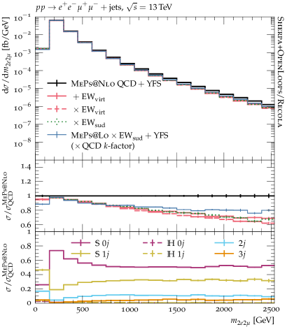
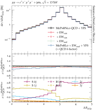
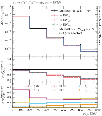
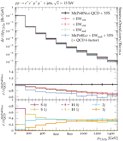
Figure 9: Distributions of leptonic observables for $pp\to e^{+}e^{-}\mu^{+}\mu^{-}+\text{jets}$ production. The baseline prediction is a MePs@Nlo calculation in the $G_{\mu}$ scheme. On top of it, $\text{EW}_{\text{virt}}$ and $\text{EW}_{\text{sud}}$ approximations are applied. As a reference, the $\text{EW}_{\text{sud}}$ approximation is also shown for an underlying MePs@Lo calculation, which is rescaled to the total MePs@Nlo rate using the global QCD $k$-factor of 1.20. The four observables shown from top left to bottom right are: the invariant mass of the four-lepton system $m_{2e2\mu}$, the $Z$-boson distance $\Delta R_{2e,2\mu}$, the transverse momentum of the di-electron pair $p_{\mathrm{T},2e}$, and the transverse momentum of the four-lepton system $p_{\mathrm{T},2e2\mu}$. All predictions are calculated using Sherpa+O PEN L OOPS /Recola. The first ratio plot shows the relative size of the EW corrections, while the second one gives the relative size of the contributions to the MePs@Nlo prediction.

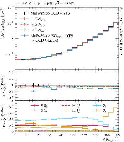
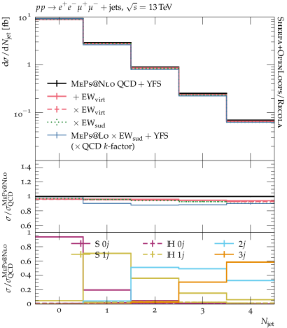
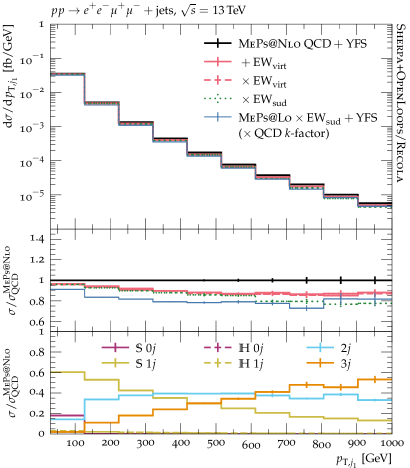
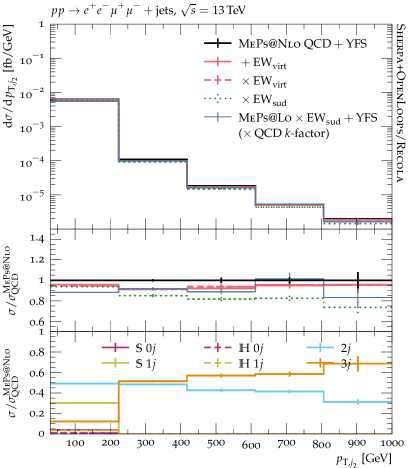
Figure 10: As Fig. 9 but for jet observables. Shown are from top left to bottom right: the angular separation between the four-lepton system and the hardest jet $\Delta\phi_{4\ell,j_{1}}$, the number of jets $N_{\text{jet}}$, and the transverse momenta of the hardest jet $p_{\text{T},j_{1}}$ and second hardest jet $p_{\text{T},j_{2}}$.

Before turning to more exclusive observables, we briefly recapitulate the key differences of how $\text{EW}_{\text{virt}}$ and $\text{EW}_{\text{sud}}$ is applied to an underlying MePs@Nlo calculation. As described in Sec. 3.2, the two approximations act differently on the individual contributions that make up a multijet-merged calculation, namely the $\mathbb{S}$ and $\mathbb{H}$ events of each QCD NLO multiplicity (here $0j$ and $1j$), and the tree-level events of the LO multiplicities (here $2j$ and $3j$). In particular, the $\text{EW}_{\text{virt}}$ is not applied to $\mathbb{H}$-type events, and approximately treats higher-multiplicity tree-level contributions through the $k$-factor defined in Eq. (3.12), such that the corrections for additional LO jets in the EW Sudakov regime are incomplete. The $\text{EW}_{\text{sud}}$ approximation on the other hand is applied to all contributions of the calculation. Therefore, we show and discuss in the following not only the baseline MePs@Nlo prediction along with the two EW approximations, but also the relative size of each contribution within the MePs@Nlo result. This helps to better understand how the MePs@Nlo results are affected by the EW approximations, and in particular to ensure that the $\text{EW}_{\text{virt}}$ approximation is not spoiled by a large admixture of $\mathbb{H}$ events.

In Fig. 9 we show the same lepton observables we examined already for the fixed-order $ZZ$ and $ZZj$ predictions presented in Sec. 4.3, here for the inclusive event selection placing no requirements on any additional jet activity, while Fig. 10 shows four observables demanding one or more additional jets beyond the inclusive lepton acceptance cuts. The latter are the angular separation $\Delta\phi_{4\ell,j_{1}}$ between the four-lepton system and the leading jet, the jet multiplicity $N_{\text{jet}}$, and the transverse momenta $p_{\mathrm{T},j_{1}}$ and $p_{\mathrm{T},j_{2}}$ of the leading and subleading jet, respectively.

Examining Figs. 9 and 10, we find the same qualitative behaviour as in the fixed-order $ZZ$ and $ZZj$ results: Distributions that have an energy scaling, such as the invariant mass of the four-lepton system, the $p_{T}$ of the leptons or that of the jets, show enhanced EW effects at high energies, which are similarly described by both the $\text{EW}_{\text{virt}}$ and $\text{EW}_{\text{sud}}$ approximations. On the other hand, scale-less quantities, such as the distance between the two $Z$-bosons or between the four-lepton system and the hardest jet, exhibit roughly flat and small corrections in both cases. This is also the case for the $N_{\mathrm{jet}}$ distribution. The reason can be seen in the fact that extra QCD radiation is predominantly soft and collinear, and as such it does neither substantially change the EW charge distribution, nor induce additional large scales.

Turning now to the various contributions of the merged calculation (as shown in the bottom panel of each plot), we can see that in all cases the contributions of $\mathbb{H}$-type events are below $5\text{\,}\mathrm{\char 37\relax}$. Therefore, the $\text{EW}_{\text{virt}}$ correction is not hampered by a large admixture of (uncorrected) $\mathbb{H}$ events in the phase space explored here. This is not surprising, because the contribution of $\mathbb{H}$ events is constrained by the $\Theta(Q_{\text{cut}}-Q_{n+1})$ term in Eq. (3.5), to avoid double counting with matrix elements of higher jet multiplicities. There is however a sizeable contribution (more than $20\text{\,}\mathrm{\char 37\relax}$) of tree-level $2j$ and/or $3j$ contributions for $\Delta R_{2e2\mu}<\pi$, $\Delta\phi_{4\ell,j_{1}}<\pi$, $N_{\text{jet}}>1$ and all transverse-momentum distributions, i.e. whenever the observable favours contributions from events with many hard and/or widely separated jets, which are mainly generated by the $2j$ and $3j$ matrix elements. While the $\text{EW}_{\text{virt}}$ falls back on the use of a $k$-factor for these two contributions, we do not find evidence that the $\text{EW}_{\text{virt}}$ and the $\text{EW}_{\text{sud}}$ generally begin to deviate from one another in the regions dominated by high-multiplicity matrix elements, suggesting that the use of a lower multiplicity (here: $1j$) to calculate approximate EW corrections via the $k$-factor does not introduce a large error for the observables studied here, as is proven in App. B.

Finally, for the MePs@Lo+$\text{EW}_{\text{sud}}$ calculation rescaled with the global QCD $k$-factor, we find that it faithfully reproduces the MePs@Nlo calculation in phase-space regions dominated by $0j$ events, while it otherwise deviates by up to $10\text{\,}\mathrm{\char 37\relax}$ from it. We have checked that this deviation is entirely due to the underlying QCD description. The $\text{EW}_{\text{sud}}$ corrections of both calculations are indeed nearly identical, which is expected given the structure of the corrections as laid out in Sec. 3.2 and the fact that the contribution of $\mathbb{H}$ events is negligible; for the $\text{EW}_{\text{sud}}$ approximation it does not matter if it is applied to LO or $\mathbb{S}$ events. The finding that $\text{EW}_{\text{sud}}$ gives identical corrections in both cases indeed serves as an important cross-check of our implementation.

Final results

After the structural analysis of the multijet-merged calculation with respect to the inclusion of EW corrections through the $\text{EW}_{\text{virt}}$ and $\text{EW}_{\text{sud}}$ approximation, we are now ready to present our final results, which are directly relevant for comparisons to data. To this end, we adjust our predictions with respect to the previous section as follows:

• The MePs@Nlo calculation remains the reference result, but we add a scale-variation band to estimate its theoretical uncertainty related to the choice of the QCD renormalisation and factorisation scales $\mu_{\mathrm{R}}$ and $\mu_{\mathrm{F}}$. The band is defined as the envelope of the 7-point variations [135]

  $$\left\{(\tfrac{1}{2}\mu_{\mathrm{R}},\;\tfrac{1}{2}\mu_{\mathrm{F}}),\;(\tfrac{1}{2}\mu_{\mathrm{R}},\mu_{\mathrm{F}}),\;(\mu_{\mathrm{R}},\tfrac{1}{2}\mu_{\mathrm{F}}),\;(\mu_{\mathrm{R}},\mu_{\mathrm{F}}),\;(\mu_{\mathrm{R}},2\mu_{\mathrm{F}}),\;(2\mu_{\mathrm{R}},\mu_{\mathrm{F}}),\;(2\mu_{\mathrm{R}},2\mu_{\mathrm{F}})\right\}\,,$$

  that are evaluated using on-the-fly reweighting [136]. The $\alpha_{\text{S}}$ and PDF input scales in the parton shower are varied along with the $\mu_{\mathrm{R}}$ and $\mu_{\mathrm{F}}$ values used in the hard process. Comparing the QCD scale uncertainties with the size of the EW corrections allows us to assess the phenomenological relevance of the latter.

• As a second addition in the QCD sector, we provide a MePs@Loop² prediction, merging loop-induced matrix elements for $ZZ$ and $ZZj$ production at LO. This is added to the MePs@Nlo calculation.

• We drop the additive $\text{EW}_{\text{virt}}$ scheme, which has been discussed in the previous section. It suffices here to consider the multiplicative scheme for further comparison. As before, we show the $\text{EW}_{\text{sud}}$ approximation, however, now supplemented with its exponentiated version, $\text{EW}_{\text{sud}}^{\text{exp}}$.

We begin by considering in Fig. 11 the four leptonic observables studied before already, i.e. $m_{2e2\mu}$, $p_{\text{T},2e}$, $\Delta R_{2e2\mu}$, and $p_{\mathrm{T},2e2\mu}$. As these are all non-zero at leading-order, in our MEPS@NLO setup they are all described at NLO QCD accuracy, receiving additional contributions also from higher-order terms. The decomposition of the MEPS@NLO prediction for the considered observables can be read off from the lower panels of Fig. 9. Notably, phase-space regions that are either filled only in the presence of, or receive large contributions from, additional radiation from either the parton shower or higher-multiplicity tree-level processes exhibit somewhat larger scale uncertainties of $\mathcal{O}{\left(\pm$10\text{\,}\%$\right)}$. This is in particular the case for $\Delta R_{2e2\mu}<\pi$ and $p_{\mathrm{T},2e2\mu}>$100\text{\,}\mathrm{G}\mathrm{e}\mathrm{V}$$, where the four-lepton system recoils against (several) additional hard emissions. For the bulk of the considered observable distributions, scale uncertainties are well below $10\text{\,}\%$. Accordingly, we find that they do not cover the EW corrections for the dimensionful observables, i.e. the transverse-momentum and invariant-mass variables, beyond scales of about $200\text{\,}\mathrm{GeV}$. For the $\Delta R_{2e2\mu}$ observable, however, where EW corrections are very moderate, they are amlost entirely covered by the QCD scale-uncertainty band.

In Fig. 12 we compile our final predictions for the jet observables, i.e. $\Delta\phi_{4\ell,j_{1}}$, $N_{\text{jet}}$, $p_{\text{T},j_{1}}$ and $p_{\text{T},j_{2}}$. Looking back at Fig. 10, we find that they are all rather dominated by the shower-evolved $2j$ and $3j$ LO matrix-element contributions, with the exception of $\Delta\phi_{4\ell,j_{1}}\gtrsim$150\text{\,}\mathrm{\SIUnitSymbolDegree}$$, $N_{\text{jet}}\leq 2$, or $p_{\text{T},j_{1}}\lesssim$100\text{\,}\mathrm{GeV}$$. The scale-uncertainty pattern is largely determined by the dominance of the higher-multiplicity LO contributions. Accordingly, we observe more significant scale variations than for the more inclusive leptonic observables. On average, the bands spread from $-10\text{\,}\mathrm{\char 37\relax}$ to $+$20\text{\,}\mathrm{\char 37\relax}$$ around the nominal MePs@Nlo prediction. For the phase-space region dominated by the NLO QCD contributions, this shrinks to $\pm$5\text{\,}\mathrm{\char 37\relax}$$, while for $N_{\text{jet}}=4$ it grows to $-$20\text{\,}\mathrm{\char 37\relax}$$ and $+$30\text{\,}\mathrm{\char 37\relax}$$. However, beyond $N_{\text{jet}}=3$ we entirely rely on the parton shower to generate additional jets.

Given the sizeable scale uncertainty of the MePs@Nlo prediction, the rather mild EW corrections observed for the $\Delta\phi_{4\ell,j_{1}}$ and $N_{\text{jet}}$ observable, which remain below $-$10\text{\,}\mathrm{\char 37\relax}$$ throughout, are fully enclosed by the QCD uncertainty band. However, for the transverse-momentum distributions EW Sudakov corrections exceed the QCD uncertainties, reaching about $-$20\text{\,}\%$$. This clearly shows the necessity to include them in realistic simulations. To further reduce the systematic uncertainties of the predictions, the two- and three-jet multiplicity matrix elements should ideally be considered at NLO QCD as well.

For all observables considered here, the shapes of the MePs@Nlo and MePs@Nlo ${}+{}$MePs@Loop² predictions are quite similar, with the latter being enhanced by about 5–$10\text{\,}\mathrm{\char 37\relax}$. The exception are the hard tails for the $p_{\text{T},2e2\mu}$, $p_{\mathrm{T,j_{1}}}$ and $p_{\mathrm{T,j_{2}}}$ distributions. Here, the cross section is with increasing hardness increasingly dominated by the MePs@Nlo contributions alone. These contain additional higher-multiplicity LO QCD matrix elements that are also the adequate sequel for the loop-induced sample, as long as no two-jet loop-induced contribution is included. The addition of the MePs@Loop² prediction has no sizeable effect on the overall QCD scale-uncertainty band of the MePs@Nlo prediction (beyond the rescaling induced by the increased rate).

As for the exponentiated $\text{EW}_{\text{sud}}$ approximation we find that it gives nearly identical results compared to the MePs@Nlo+$\text{EW}_{\text{sud}}$ one, due to the moderate absolute $\text{EW}_{\text{sud}}$ correction for the studied observables.

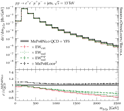
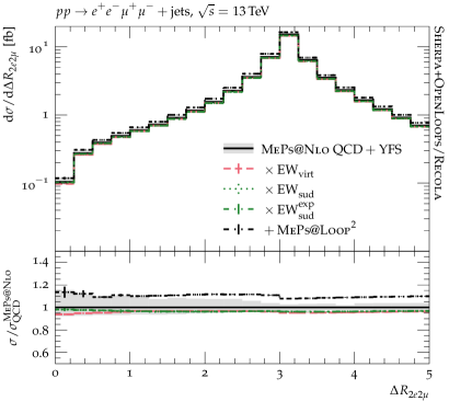
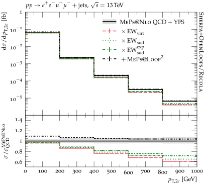
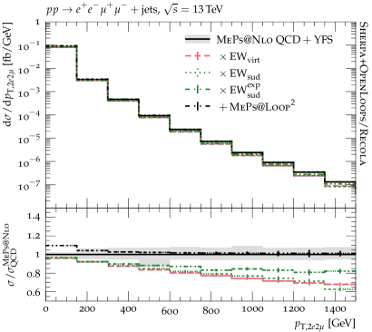
Figure 11: Distributions of leptonic observables for $pp\to e^{+}e^{-}\mu^{+}\mu^{-}+\text{jets}$ production. The baseline prediction is given by the MePs@Nlo result in the $G_{\mu}$ scheme, with the grey band indicating its 7-point scale-variation uncertainty. On top of it, loop-induced corrections and $\text{EW}_{\text{virt}}$/$\text{EW}_{\text{sud}}$ approximations are applied. Shown are from top left to bottom right: the four-lepton invariant mass $m_{2e2\mu}$, the $Z$-boson distance $\Delta R_{2e,2\mu}$, the di-electron transverse momentum $p_{\text{T},2e}$, and four-lepton transverse momentum $p_{\text{T},2e2\mu}$. All predictions are calculated using Sherpa+O PEN L OOPS /Recola.

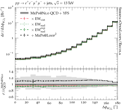
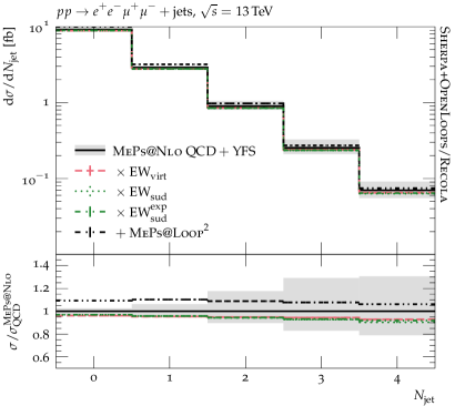
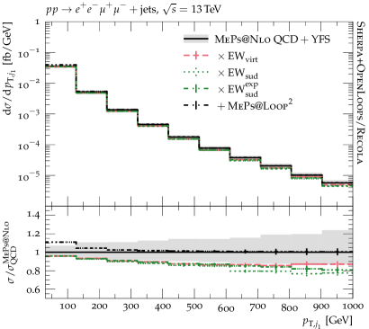
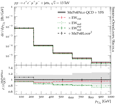
Figure 12: As Fig. 11 but for jet observables. Shown are from top left to bottom right: the angular separation between the four-lepton system and the hardest jet $\Delta\phi_{4\ell,j_{1}}$, the number of jets $N_{\text{jet}}$, and the transverse momenta of the hardest jet $p_{\text{T},j_{1}}$ and second hardest jet $p_{\text{T},j_{2}}$.

5 Conclusions

To adequately address precision measurements of final states produced in hadronic collisions, the inclusion of higher-order corrections in corresponding theoretical predictions based on perturbation theory is required. Besides the dominant QCD contributions, typically considered at NLO or NNLO, also EW corrections should ideally be included, certainly when attempting to describe phase-space regions involving high-energetic particles. In this limit the exact NLO EW corrections factorise from the production process, leading to logarithms of the involved kinematic invariants that can eventually be resummed to all orders.

In this article we discussed the means to compute EW corrections at exact NLO accuracy, as well as the high-energy virtual EW ($\text{EW}_{\text{virt}}$) and Sudakov ($\text{EW}_{\text{sud}}$) approximations, in the Sherpa framework. We have presented a simple matching formula for the combination of resummed NLL EW Sudakov corrections with the exact $\mathcal{O}{\left(\alpha\right)}$ result. This NLO EW${}+{}$NLL $\text{EW}_{\text{sud}}^{\text{exp}}$ calculation enables us to account for the dominant EW corrections both in the bulk of the inclusive cross section as well as for high-energetic kinematic configurations. Properly modelling multiple QCD parton emissions off the initial and final state of the process requires the inclusion of parton-shower simulations, i.e. the matching and merging of QCD matrix elements with a QCD parton cascade. Such methods for LO and NLO matrix elements are readily available in Sherpa, referred to as MePs@Lo and MePs@Nlo, respectively. However, the consistent inclusion of (approximate) EW corrections in such shower-evolved computations is an area of active theoretical development. In our work we have presented the methods available in Sherpa for the largely automated incorporation of EW corrections in MePs@Lo and MePs@Nlo calculations. This includes in particular the $\text{EW}_{\text{virt}}$ approximation for $\mathcal{O}{\left(\alpha\right)}$ corrections, and the more recently implemented $\text{EW}_{\text{sud}}$ scheme for including (resummed) NLL EW contributions. Both approaches can consistently be combined with QED soft-photon resummation for final-state leptons, treated in the YFS formalism.

As an highly non-trivial application and benchmark for the various calculational schemes we analysed $ZZ$ and $ZZj$ production under LHC conditions, thereby including off-shell and non-resonant contributions to the $e^{+}e^{-}\mu^{+}\mu^{-}$ and $e^{+}e^{-}\mu^{+}\mu^{-}j$ channels, respectively. For the first time we have presented results for detailed kinematical distributions for $pp\to e^{+}e^{-}\mu^{+}\mu^{-}j$ at NLO EW. In a first analysis we studied the quality of the $\text{EW}_{\text{virt}}$ and $\text{EW}_{\text{sud}}$ schemes in approximating the exact NLO EW results, with one-loop amplitudes provided by O PEN L OOPS and Recola. For both the $ZZ$ and the $ZZj$ channel we found a correction of the inclusive fiducial cross section from LO to NLO of about $-7\text{\,}\%$ when using the $G_{\mu}$ input-parameter and renormalisation scheme. This effect is well reproduced by the $\text{EW}_{\text{virt}}$ and $\text{EW}_{\text{sud}}$ approximations when combined with the YFS soft-photon resummation. While for the considered inclusive cross sections the exponentiation of the NLL Sudakov logarithms has only a very mild effect, it significantly alters the production rate of high-energetic event configurations, e.g. when applying a hard cut on the transverse momentum of one of the $Z$ bosons. Through matching to the exact NLO EW result these higher-order EW effects can be incorporated in the combined prediction of NLO EW${}+{}$NLL $\text{EW}_{\text{sud}}^{\text{exp}}$ accuracy.

Motivated by the good quality of the EW virtual and Sudakov approximation for the diboson-production processes, we then considered their inclusion in MePs@Nlo  predictions based on the NLO QCD matrix elements for the zero- and one-jet channel, supplemented by the tree-level two- and three-jet processes. Both for the inclusive production rates and for the considered differential distributions, we found good agreement of the resulting MePs@Nlo+$\text{EW}_{\text{sud}}$ and MePs@Nlo+$\text{EW}_{\text{virt}}$ predictions. Only for phase-space regions dominated by the higher-order tree-level contributions did we observe systematic deviations. These can be traced back to the limitation of the $\text{EW}_{\text{virt}}$  approximation to model the EW corrections for these tree-level contributions through an effective $k$-factor corresponding to the highest-multiplicity available at NLO, here the one-jet process. In the $\text{EW}_{\text{sud}}$ approximation, however, higher-order tree-level processes with kinematics in the high-energy regime receive the complete NLL EW Sudakov factor. Having analysed in detail the anatomy of the multijet-merged samples with EW corrections included, we presented our final phenomenological predictions, thereby also including an uncertainty estimate corresponding to scale variations and taking into account the QCD loop-induced contributions to $ZZ$ and $ZZj$ production. The loop-induced channels contribute at the order of $10\text{\,}\%$ of the total production rate only. Accordingly, neglecting their EW corrections seems well justified. However, we could clearly show that EW corrections for the direct production mode—in particular for high-energetic event configurations—amount to up to $-40\text{\,}\%$, and thereby largely exceed the QCD scale uncertainty of the MePs@Nlo computation.

Accordingly, the inclusion of EW corrections in theoretical predictions is of paramount importance for upcoming measurements of diboson production at the LHC in Run 3 and the subsequent High-Luminosity phase. This applies both to fixed-order calculations and to fully differential multijet-merged Monte Carlo simulations to be used in precision Standard Model studies. The inclusion is similarly important for analyses in which these processes contribute as Standard Model background to New Physics searches.also Consequently, the methods developed here, due to their automation in the Sherpa framework, can and should be applied to any other process. They will be publicly available with Sherpa-3.

Appendix A EW Sudakov corrections outside the strict high-energy limit

Following [41, 42], the strict condition of the high-energy limit that all invariants $r_{kl}=(p_{k}+p_{l})^{2}$ with external momenta $p_{k}$ and $p_{l}$ are large compared to the EW energy scale has the consequence that a naive application to processes with intermediate resonances, such as $W$ and $Z$ bosons decaying into leptons, will result in $\delta_{\text{sud},n}^{\text{EW}}=\mathrm{K}_{\text{sud},n}^{\text{NLL}}=0$. This is because the intermediate resonance will constrain the invariant mass of the decay products $k$ and $l$ to be close to its on-shell mass. In consequence, at least this $r_{kl}$ is of the order of the EW scale and not large compared to it. To address this, we follow the same strategy as is used in the YFS resummation in processes with internal resonances [93, 53].

We have extended the original Sherpa implementation of Sudakov corrections presented in [44] in the following way. Before calculating $\mathrm{K}_{\text{sud},n}^{\text{NLL}}$, we combine any lepton pair $(k,l)$ with an invariant mass $m_{kl}$ close to the mass $M_{V}$ ($V=W,Z$) of a vector boson of the same quantum numbers, based on the measure

$$\Delta_{kl}=\frac{|m_{kl}-M_{V}|}{\Gamma_{V}}<\Delta_{\text{thr}}\;,$$ (A.1)

with $\Gamma_{V}$ the width of the vector boson. $\Delta_{\text{thr}}$ is an arbitrary threshold parameter that we set to $10$. If multiple possible combinations exist, e.g. in $e^{+}e^{+}e^{-}e^{-}$ final states, the pair with the smallest $\Delta_{kl}$ is combined first. The resulting amplitude now has $m\leq n$ external particles. Note that this also implies that the phase space used to evaluate the EW Sudakov contribution changes as well, and it now refers to $m\leq n$ (or $m\leq n+1$ for $\mathbb{H}$ events) final-state particles, with $m$ depending on the number of combined lepton pairs. We then set $\delta_{\text{sud},n}^{\text{EW}}\left(\Phi_{n}\right)=\mathrm{K}_{\text{sud},m}^{\text{NLL}}\left(\Phi_{m}\right)$. The clustered phase space $\Phi_{m}$ is constructed by combining the four momenta of all clustered lepton pairs ($k$, $l$), and assign it to new external vector bosons, i.e. $p_{V,kl}=p_{k}+p_{l}$. After all possible daughter leptons are clustered, all momenta in $\Phi_{m}$ are reshuffled such that all external particles are on their mass shell, in particular $p^{2}_{V,kl}=m^{2}_{V}$. To this end, we use the same algorithm as in Ref. [44] to ensure that all matrix elements entering the calculation of $\mathrm{K}_{\text{sud},n}^{\text{NLL}}$ have on-shell external momenta after potential $\text{SU}(2)$ rotations of external states, see the discussion therein.

As a second provision to improve the $\text{EW}_{\text{sud}}$ approximation in phase-space regions where not all invariants are of the same large size, we include terms proportional to

$$L(|r_{kl}|,s)=\frac{\alpha}{4\pi}\log^{2}\left(\frac{r_{kl}}{s}\right)\;,$$ (A.2)

as they appear in the split of the double logarithmic (DL) terms in [41]. Here, $s$ is the squared partonic centre-of-mass energy. The terms in Eq. (A.2) are neglected in [41] and in our original implementation [44], as the strict high-energy limit requires $M_{W}^{2}\ll r_{kl}\sim s$. However, we find that in the $ZZ$ and $ZZj$ observables studied here neglecting these terms consistently reduces the level of agreement between $\text{EW}_{\text{sud}}$ and NLO EW by up to $5\text{\,}\mathrm{\char 37\relax}$, due to the contribution of kinematic configurations where at least for some invariants a looser high-energy limit $M_{W}^{2}\ll r_{kl}\ll s$ is approached.

Hence, we have included these contributions in all $\text{EW}_{\text{sud}}$ results and made this behaviour the new default of the implementation in Sherpa. Note that this term is also retained in [45] as part of the so-called $\mathrm{SSC}^{{s\rightarrow r}_{kl}}$ contribution.

Appendix B Matched EW corrections in multijet-merged calculations

This appendix discusses how the interplay of the EW corrections contained in the local $k$-factor and those explicitly effected onto the higher-multiplicity LO matrix elements achieves both the correct resummation of the multiplicity-specific EW Sudakov factors and the inclusive behaviour of the $\text{EW}_{\text{virt}}$ approximation of the highest multiplicity it is available for. Thus, it needs to be shown that the EW corrections for a) the $n=n_{\text{max}}^{\text{NLO}}$ parton process are not changed when higher-multiplicity LO matrix elements are merged on top of it, and b) the $n=n_{\text{max}}^{\text{NLO}}+l$ parton processes properly resum their respective Sudakov logarithms.

First, we show that for the highest multiplicity for which NLO EW virtual corrections are available, $n=n_{\text{max}}^{\text{NLO}}$, the correction effected onto observables sensitive to it are given by the matched EW corrections of Eq. (3.18). To this end, we examine the inclusive $n$-parton cross section consisting of the sum of the exclusive $n$-parton cross section and the inclusive $(n+1)$-parton cross section. Further splitting the latter into the exclusive $(n+1)$-parton cross section and the inclusive $(n+2)$-parton cross section follows trivially and does not change our conclusions. The inclusive $n$-parton cross section, integrating over both unresolved and resolved emissions (according to the merging scale), is then given by

$$\begin{split}\mathrm{d}\sigma_{n}^{\text{{MePs@Nlo}}}=&\;\mathrm{d}\Phi_{n}\,\overline{\mathrm{B}}_{n}(\Phi_{n})\,\left[\exp\left(\delta_{\text{sud},n}^{\text{EW}}(\Phi_{n})\vphantom{\frac{\pi^{2}}{6}}\right)-\delta_{\text{sud},n}^{\text{EW}}(\Phi_{n})+\delta_{\text{virt},n,\mathbb{S}}^{\text{EW}}(\Phi_{n})\right]\,\Theta_{n}(Q_{\text{cut}})\\ &\times\left\{\overline{\Delta}_{n}(t_{c},t_{n})\vphantom{\int\limits_{A}^{B}}\right.\\ &\hskip 15.0pt\left.{}+\int_{t_{c}}^{t_{n}}\!\!\mathrm{d}\Phi_{1}^{\prime}\,\overline{\mathrm{K}}_{n}\left(\Phi_{1}^{\prime}\right)\left[\overline{\Delta}_{n}(t_{n+1}^{\prime},t_{n})\,\Theta(Q_{\text{cut}}-Q_{n+1}^{\prime})\vphantom{\frac{\left(\delta_{\text{sud},n}^{\text{EW}}\right)}{\left(\delta_{\text{sud},n}^{\text{EW}}\right)}}\right.\right.\\ &\left.\left.\hskip 105.0pt{}+\frac{\exp\left(\delta_{\text{sud},n+1}^{\text{EW}}(\Phi_{n+1}^{\prime})\vphantom{\frac{\pi^{2}}{6}}\right)}{\exp\left(\delta_{\text{sud},n}^{\text{EW}}(\Phi_{n})\vphantom{\frac{\pi^{2}}{6}}\right)}\,\Delta_{n}(t_{n+1}^{\prime},t_{n})\,\Theta(Q_{n+1}^{\prime}-Q_{\text{cut}})\right]\right.\\ &\left.\hskip 60.0pt{}\times\mathcal{F}_{n+1}(t_{n+1}^{\prime})\vphantom{\frac{\left(\delta_{\text{sud},n}^{\text{EW}}\right)}{\left(\delta_{\text{sud},n}^{\text{EW}}\right)}}\right\}\\ &{}+\mathrm{d}\Phi_{n+1}\,\mathrm{H}_{n}(\Phi_{n+1})\,\exp\left(\delta_{\text{sud},n+1}^{\text{EW}}(\Phi_{n+1})\vphantom{\frac{\pi^{2}}{6}}\right)\,\Theta_{n}(Q_{\text{cut}})\,\mathcal{F}_{n+1}(\mu_{Q}^{2},Q_{\text{cut}})\;,\end{split}$$ (B.1)

with $\Phi_{n+1}^{\prime}=\Phi_{n}\cdot\Phi_{1}^{\prime}$ and where we have explicitly extracted the relevant Sudakov factor from the vetoed parton shower where appropriate. The only offending term with respect to the pure unmerged result is the ratio of the $n$- and $(n+1)$-parton Sudakov factor above the merging scale, brought about by the local $k$-factor of Eq. (3.19) acting on the LO $(n+1)$-parton process. This factor, however, is of $\mathcal{O}{\left(\alpha_{s}\right)}$ (contained in the modified splitting kernel $\overline{\mathrm{K}}_{n}$) relative to the intended accuracy of the matched result in the $n$-parton phase space. Further, for $Q_{n+1}$ around the merging scale $Q_{\text{cut}}$, the ratio of Sudakov factors is near unity as a relatively soft $(n+1)$st emission does not contribute any large invariants to the existing $n$-parton ensemble. For $Q_{n+1}\gg Q_{\text{cut}}$, where the $(n+1)$st emission does contribute large invariants to the process, we are in the Sudakov limit where $\delta_{\text{sud},n}^{\text{EW}}$ and $\delta_{\text{virt},n}^{\text{EW}}$ coincide and, thus, this ratio replaces the $n$-parton resummed Sudakov corrections with the more suitable $(n+1)$-parton resummed Sudakov corrections, a clear improvement over the unmerged result. As a short aside, it is interesting to note that in case of the pure $\text{EW}_{\text{virt}}$ approximation of Eq. (3.11) or (3.13) this ratio of Sudakov factors is absent and the exact unmerged result for the $n$-parton process is reproduced by the merged calculation.

Second, we show that observables sensitive to $(n+l)$-parton processes with $l>0$ are exposed to the correct $(n+l)$-parton resummed Sudakov correction in the Sudakov regime. We examine this explicitly for $l=1$, and the higher-multiplicity processes follow by analogy. We thus have

$$\begin{split}\mathrm{d}\sigma_{n+1}^{\text{{MePs@Nlo}}}=&\;\mathrm{d}\Phi_{n+1}\,\mathrm{B}_{n+1}(\Phi_{n+1})\,\exp\left(\delta_{\text{sud},n+1}^{\text{EW}}(\Phi_{n+1})\vphantom{\frac{a}{a}}\right)\,\Theta_{n}(Q_{\text{cut}})\,\mathcal{F}(\mu_{Q}^{2},Q_{\text{cut}})\\ &{}+\mathrm{d}\Phi_{n+1}\,\mathrm{D}_{n}(\Phi_{n+1})\,\exp\left(\delta_{\text{sud},n+1}^{\text{EW}}(\Phi_{n+1})\vphantom{\frac{a}{a}}\right)\,\Theta_{n}(Q_{\text{cut}})\vphantom{\int_{A}^{B}}\\ &\hskip 10.0pt\times\left\{\frac{\overline{\mathrm{B}}_{n}(\Phi_{n})}{\mathrm{B}_{n}(\Phi_{n})}\left(1-\frac{\delta_{\text{sud},n}^{\text{EW}}(\Phi_{n})-\delta_{\text{virt},n}^{\text{EW}}(\Phi_{n})}{\exp\left(\delta_{\text{sud},n}^{\text{EW}}(\Phi_{n})\vphantom{\frac{a}{a}}\right)}\right)\right.\\ &\hskip 70.0pt\left.\times\left[\frac{\exp\left(\delta_{\text{sud},n}^{\text{EW}}(\Phi_{n})\vphantom{\frac{\pi^{2}}{6}}\right)}{\exp\left(\delta_{\text{sud},n+1}^{\text{EW}}(\Phi_{n+1})\vphantom{\frac{a}{a}}\right)}\;\overline{\Delta}_{n}(t_{n+1},t_{n})\,\Theta(Q_{\text{cut}}-Q_{n+1})\right.\right.\\ &\hskip 85.0pt\left.\left.{}+\Delta_{n}(t_{n+1},t_{n})\,\Theta(Q_{n+1}-Q_{\text{cut}})\vphantom{\int\limits_{A}^{B}}\right]\;\;-\;1\;\;\vphantom{\int\limits_{A}^{B}}\right\}\;\mathcal{F}_{n+1}(t_{n+1})\;.\end{split}$$ (B.2)

While the term of the first line represents the desired result, the second term is, in the absence of EW corrections, a correction of relative $\mathcal{O}{\left(\alpha_{s}\right)}$ ($\overline{\mathrm{B}}_{n}/\mathrm{B}_{n}=1+\mathcal{O}{\left(\alpha_{s}\right)}$), applied in the region where the $(n+1)$-parton matrix element can be written as an $n$-parton matrix element times a splitting kernel, $\mathrm{D}_{n}=\mathrm{B}_{n}\overline{\mathrm{K}}_{n}\,\Theta(\mu_{Q}^{2}-t_{n+1})$, reproducing the behaviour of the unmerged result, see [101]. In the presence of EW corrections, however, the situation is slightly more involved, leading nonetheless to the same conclusion. First, we observe again that for small emission scales $Q_{n+1}$ the $(n+1)$st parton does not produce additional large invariants with respect to those of the $n$-parton ensemble, thus $\delta_{\text{sud},n}^{\text{EW}}(\Phi_{n})\approx\delta_{\text{sud},n+1}^{\text{EW}}(\Phi_{n+1})$. The ratio of Sudakov factors appearing in the fourth line for emissions below the merging scale $Q_{\text{cut}}$ therefore vanishes in this region, letting the square bracket sum up to unity up to terms of subleading colour at relative $\mathcal{O}{\left(\alpha_{s}\right)}$, as in the pure QCD case. In consequence, the curly bracket produces a term of $\mathcal{O}{\left(\alpha\right)}$ in addition to the pure QCD case, containing the ratio of the difference of the $\text{EW}_{\text{sud}}$ and $\text{EW}_{\text{virt}}$ approximations and the resummed Sudakov corrections in the underlying $n$-parton phase space. This term simply replaces the $\mathcal{O}{\left(\alpha\right)}$ expansion of the resummed $n$-parton Sudakov correction underlying the resummed $(n+1)$-parton Sudakov correction in the $\mathrm{D}_{n}$ part of $\mathrm{B}_{n+1}$ of the first line ($\mathrm{B}_{n+1}=\mathrm{D}_{n}+\mathrm{H}_{n}$), $\delta_{\text{sud},n}^{\text{EW}}$, with $\delta_{\text{virt},n}^{\text{EW}}$. As both $\text{EW}_{\text{virt}}$ and $\text{EW}_{\text{sud}}$ coincide in the Sudakov limit, the EW Sudakov logarithms of the appropriate $(n+1)$-parton phase space are resummed unimpededly. On the other hand, in the inclusive phase space, this construction benefits at least in part from the additional terms contained in the $\text{EW}_{\text{virt}}$ approximation of the underlying $n$-parton phase-space configuration.

References

- [1] R. D. Ball et al., The Path to Proton Structure at One-Percent Accuracy, arXiv:2109.02653 [hep-ph]
- [2] A. Denner and S. Dittmaier, Electroweak Radiative Corrections for Collider Physics, Phys. Rept. 864 (2020), 1–163, [arXiv:1912.06823 [hep-ph]]
- [3] G. Cullen et al., GS-2.0: a tool for automated one-loop calculations within the Standard Model and beyond, Eur. Phys. J. C 74 (2014), no. 8, 3001, [arXiv:1404.7096 [hep-ph]]
- [4] V. Hirschi, R. Frederix, S. Frixione, M. V. Garzelli, F. Maltoni and R. Pittau, Automation of one-loop QCD corrections, JHEP 05 (2011), 044, [arXiv:1103.0621 [hep-ph]]
- [5] R. Frederix, S. Frixione, V. Hirschi, D. Pagani, H. S. Shao and M. Zaro, The automation of next-to-leading order electroweak calculations, JHEP 07 (2018), 185, [arXiv:1804.10017 [hep-ph]]
- [6] J. M. Campbell, D. Wackeroth and J. Zhou, Study of weak corrections to Drell-Yan, top-quark pair, and dijet production at high energies with MCFM, Phys. Rev. D 94 (2016), no. 9, 093009, [arXiv:1608.03356 [hep-ph]]
- [7] S. Honeywell, S. Quackenbush, L. Reina and C. Reuschle, NLOX, a one-loop provider for Standard Model processes, Comput. Phys. Commun. 257 (2020), 107284, [arXiv:1812.11925 [hep-ph]]
- [8] F. Buccioni, J.-N. Lang, J. M. Lindert, P. Maierhöfer, S. Pozzorini, H. Zhang and M. F. Zoller, OpenLoops 2, Eur. Phys. J. C 79 (2019), no. 10, 866, [arXiv:1907.13071 [hep-ph]]
- [9] S. Actis, A. Denner, L. Hofer, J.-N. Lang, A. Scharf and S. Uccirati, RECOLA: REcursive Computation of One-Loop Amplitudes, Comput. Phys. Commun. 214 (2017), 140–173, [arXiv:1605.01090 [hep-ph]]
- [10] S. Catani and M. H. Seymour, A General algorithm for calculating jet cross-sections in NLO QCD, Nucl. Phys. B 485 (1997), 291–419, [hep-ph/9605323], [Erratum: Nucl.Phys.B 510, 503–504 (1998)]
- [11] S. Catani, S. Dittmaier, M. H. Seymour and Z. Trocsanyi, The Dipole formalism for next-to-leading order QCD calculations with massive partons, Nucl. Phys. B 627 (2002), 189–265, [hep-ph/0201036]
- [12] S. Frixione, Z. Kunszt and A. Signer, Three jet cross-sections to next-to-leading order, Nucl. Phys. B 467 (1996), 399–442, [hep-ph/9512328]
- [13] S. Dittmaier, A General approach to photon radiation off fermions, Nucl. Phys. B 565 (2000), 69–122, [hep-ph/9904440]
- [14] S. Dittmaier, A. Kabelschacht and T. Kasprzik, Polarized QED splittings of massive fermions and dipole subtraction for non-collinear-safe observables, Nucl. Phys. B 800 (2008), 146–189, [arXiv:0802.1405 [hep-ph]]
- [15] T. Gleisberg and F. Krauss, Automating dipole subtraction for QCD NLO calculations, Eur. Phys. J. C 53 (2008), 501–523, [arXiv:0709.2881 [hep-ph]]
- [16] R. Frederix, T. Gehrmann and N. Greiner, Integrated dipoles with MadDipole in the MadGraph framework, JHEP 06 (2010), 086, [arXiv:1004.2905 [hep-ph]]
- [17] T. Gehrmann and N. Greiner, Photon Radiation with MadDipole, JHEP 12 (2010), 050, [arXiv:1011.0321 [hep-ph]]
- [18] M. Schönherr, An automated subtraction of NLO EW infrared divergences, Eur. Phys. J. C78 (2018), no. 2, 119, [arXiv:1712.07975 [hep-ph]]
- [19] S. Kallweit, J. M. Lindert, P. Maierhöfer, S. Pozzorini and M. Schönherr, NLO electroweak automation and precise predictions for W+multijet production at the LHC, JHEP 04 (2015), 012, [arXiv:1412.5157 [hep-ph]]
- [20] A. Denner and M. Pellen, NLO electroweak corrections to off-shell top-antitop production with leptonic decays at the LHC, JHEP 08 (2016), 155, [arXiv:1607.05571 [hep-ph]]
- [21] F. Granata, J. M. Lindert, C. Oleari and S. Pozzorini, NLO QCD+EW predictions for HV and HV+jet production including parton-shower effects, JHEP 09 (2017), 012, [arXiv:1706.03522 [hep-ph]]
- [22] M. Chiesa, N. Greiner, M. Schönherr and F. Tramontano, Electroweak corrections to diphoton plus jets, JHEP 10 (2017), 181, [arXiv:1706.09022 [hep-ph]]
- [23] N. Greiner and M. Schönherr, NLO QCD+EW corrections to diphoton production in association with a vector boson, JHEP 01 (2018), 079, [arXiv:1710.11514 [hep-ph]]
- [24] Schönherr, Marek, Next-to-leading order electroweak corrections to off-shell WWW production at the LHC, JHEP 07 (2018), 076, [arXiv:1806.00307 [hep-ph]]
- [25] A. Denner, S. Dittmaier, P. Maierhöfer, M. Pellen and C. Schwan, QCD and electroweak corrections to WZ scattering at the LHC, JHEP 06 (2019), 067, [arXiv:1904.00882 [hep-ph]]
- [26] S. Dittmaier, G. Knippen and C. Schwan, Next-to-leading-order QCD and electroweak corrections to triple-W production with leptonic decays at the LHC, JHEP 02 (2020), 003, [arXiv:1912.04117 [hep-ph]]
- [27] D. Pagani, I. Tsinikos and E. Vryonidou, NLO QCD+EW predictions for and production at the LHC, JHEP 08 (2020), 082, [arXiv:2006.10086 [hep-ph]]
- [28] D. Pagani, H.-S. Shao, I. Tsinikos and M. Zaro, Automated EW corrections with isolated photons: , and as case studies, JHEP 09 (2021), 155, [arXiv:2106.02059 [hep-ph]]
- [29] R. Frederix, S. Frixione, V. Hirschi, D. Pagani, H.-S. Shao and M. Zaro, The complete NLO corrections to dijet hadroproduction, JHEP 04 (2017), 076, [arXiv:1612.06548 [hep-ph]]
- [30] M. Reyer, M. Schönherr and S. Schumann, Full NLO corrections to 3-jet production and at the LHC, Eur. Phys. J. C 79 (2019), no. 4, 321, [arXiv:1902.01763 [hep-ph]]
- [31] B. Biedermann, A. Denner and M. Pellen, Complete NLO corrections to W+W+ scattering and its irreducible background at the LHC, JHEP 10 (2017), 124, [arXiv:1708.00268 [hep-ph]]
- [32] A. Denner, R. Franken, M. Pellen and T. Schmidt, NLO QCD and EW corrections to vector-boson scattering into ZZ at the LHC, JHEP 11 (2020), 110, [arXiv:2009.00411 [hep-ph]]
- [33] A. Denner, R. Franken, M. Pellen and T. Schmidt, Full NLO predictions for vector-boson scattering into Z bosons and its irreducible background at the LHC, JHEP 10 (2021), 228, [arXiv:2107.10688 [hep-ph]]
- [34] J. Alwall, R. Frederix, S. Frixione, V. Hirschi, F. Maltoni, O. Mattelaer, H. S. Shao, T. Stelzer, P. Torrielli and M. Zaro, The automated computation of tree-level and next-to-leading order differential cross sections, and their matching to parton shower simulations, JHEP 07 (2014), 079, [arXiv:1405.0301 [hep-ph]]
- [35] S. Alioli, P. Nason, C. Oleari and E. Re, A general framework for implementing NLO calculations in shower Monte Carlo programs: the POWHEG BOX, JHEP 06 (2010), 043, [arXiv:1002.2581 [hep-ph]]
- [36] T. Gleisberg, S. Höche, F. Krauss, M. Schönherr, S. Schumann, F. Siegert and J. Winter, Event generation with SHERPA 1.1, JHEP 02 (2009), 007, [arXiv:0811.4622 [hep-ph]]
- [37] E. Bothmann et al., Event Generation with Sherpa 2.2, SciPost Phys. 7 (2019), no. 3, 034, [arXiv:1905.09127 [hep-ph]]
- [38] A. Buckley et al., General-purpose event generators for LHC physics, Phys. Rept. 504 (2011), 145–233, [arXiv:1101.2599 [hep-ph]]
- [39] V. V. Sudakov, Vertex parts at very high-energies in quantum electrodynamics, Sov. Phys. JETP 3 (1956), 65–71
- [40] P. Ciafaloni and D. Comelli, Sudakov enhancement of electroweak corrections, Phys. Lett. B 446 (1999), 278–284, [hep-ph/9809321]
- [41] A. Denner and S. Pozzorini, One loop leading logarithms in electroweak radiative corrections. 1. Results, Eur.Phys.J. C18 (2001), 461–480, [arXiv:hep-ph/0010201 [hep-ph]]
- [42] A. Denner and S. Pozzorini, One loop leading logarithms in electroweak radiative corrections. 2. Factorization of collinear singularities, Eur.Phys.J. C21 (2001), 63–79, [arXiv:hep-ph/0104127 [hep-ph]]
- [43] M. Chiesa, G. Montagna, L. Barzè, M. Moretti, O. Nicrosini, F. Piccinini and F. Tramontano, Electroweak Sudakov Corrections to New Physics Searches at the LHC, Phys. Rev. Lett. 111 (2013), no. 12, 121801, [arXiv:1305.6837 [hep-ph]]
- [44] E. Bothmann and D. Napoletano, Automated evaluation of electroweak Sudakov logarithms in Sherpa, Eur. Phys. J. C 80 (2020), no. 11, 1024, [arXiv:2006.14635 [hep-ph]]
- [45] D. Pagani and M. Zaro, One-loop electroweak Sudakov logarithms: a revisitation and automation, arXiv:2110.03714 [hep-ph]
- [46] S. Kallweit, J. M. Lindert, P. Maierhöfer, S. Pozzorini and M. Schönherr, NLO QCD+EW predictions for V + jets including off-shell vector-boson decays and multijet merging, JHEP 04 (2016), 021, [arXiv:1511.08692 [hep-ph]]
- [47] F. Cascioli, T. Gehrmann, M. Grazzini, S. Kallweit, P. Maierhöfer, A. von Manteuffel, S. Pozzorini, D. Rathlev, L. Tancredi and E. Weihs, ZZ production at hadron colliders in NNLO QCD, Phys. Lett. B 735 (2014), 311–313, [arXiv:1405.2219 [hep-ph]]
- [48] M. Grazzini, S. Kallweit and D. Rathlev, ZZ production at the LHC: fiducial cross sections and distributions in NNLO QCD, Phys. Lett. B 750 (2015), 407–410, [arXiv:1507.06257 [hep-ph]]
- [49] G. Heinrich, S. Jahn, S. P. Jones, M. Kerner and J. Pires, NNLO predictions for Z-boson pair production at the LHC, JHEP 03 (2018), 142, [arXiv:1710.06294 [hep-ph]]
- [50] S. Kallweit and M. Wiesemann, production at the LHC: NNLO predictions for and signatures, Phys. Lett. B 786 (2018), 382–389, [arXiv:1806.05941 [hep-ph]]
- [51] B. Biedermann, A. Denner, S. Dittmaier, L. Hofer and B. Jäger, Electroweak corrections to at the LHC: a Higgs background study, Phys. Rev. Lett. 116 (2016), no. 16, 161803, [arXiv:1601.07787 [hep-ph]]
- [52] B. Biedermann, A. Denner, S. Dittmaier, L. Hofer and B. Jäger, Next-to-leading-order electroweak corrections to the production of four charged leptons at the LHC, JHEP 01 (2017), 033, [arXiv:1611.05338 [hep-ph]]
- [53] S. Kallweit, J. M. Lindert, S. Pozzorini and M. Schönherr, NLO QCD+EW predictions for diboson signatures at the LHC, JHEP 11 (2017), 120, [arXiv:1705.00598 [hep-ph]]
- [54] M. Chiesa, A. Denner and J.-N. Lang, Anomalous triple-gauge-boson interactions in vector-boson pair production with RECOLA2, Eur. Phys. J. C 78 (2018), no. 6, 467, [arXiv:1804.01477 [hep-ph]]
- [55] M. Grazzini, S. Kallweit, J. M. Lindert, S. Pozzorini and M. Wiesemann, NNLO QCD + NLO EW with Matrix+OpenLoops: precise predictions for vector-boson pair production, JHEP 02 (2020), 087, [arXiv:1912.00068 [hep-ph]]
- [56] T. Melia, P. Nason, R. Röntsch and G. Zanderighi, W+W-, WZ and ZZ production in the POWHEG BOX, JHEP 11 (2011), 078, [arXiv:1107.5051 [hep-ph]]
- [57] R. Frederix, S. Frixione, V. Hirschi, F. Maltoni, R. Pittau and P. Torrielli, Four-lepton production at hadron colliders: aMC@NLO predictions with theoretical uncertainties, JHEP 02 (2012), 099, [arXiv:1110.4738 [hep-ph]]
- [58] M. Chiesa, C. Oleari and E. Re, NLO QCD+NLO EW corrections to diboson production matched to parton shower, Eur. Phys. J. C 80 (2020), no. 9, 849, [arXiv:2005.12146 [hep-ph]]
- [59] S. Alioli, A. Broggio, A. Gavardi, S. Kallweit, M. A. Lim, R. Nagar and D. Napoletano, Next-to-next-to-leading order event generation for boson pair production matched to parton shower, Phys. Lett. B 818 (2021), 136380, [arXiv:2103.01214 [hep-ph]]
- [60] S. Alioli, C. W. Bauer, C. J. Berggren, A. Hornig, F. J. Tackmann, C. K. Vermilion, J. R. Walsh and S. Zuberi, Combining Higher-Order Resummation with Multiple NLO Calculations and Parton Showers in GENEVA, JHEP 09 (2013), 120, [arXiv:1211.7049 [hep-ph]]
- [61] S. Alioli, C. W. Bauer, C. Berggren, F. J. Tackmann, J. R. Walsh and S. Zuberi, Matching Fully Differential NNLO Calculations and Parton Showers, JHEP 06 (2014), 089, [arXiv:1311.0286 [hep-ph]]
- [62] S. Alioli, C. W. Bauer, C. Berggren, F. J. Tackmann and J. R. Walsh, Drell-Yan production at NNLL’+NNLO matched to parton showers, Phys. Rev. D 92 (2015), no. 9, 094020, [arXiv:1508.01475 [hep-ph]]
- [63] S. Alioli, C. W. Bauer, S. Guns and F. J. Tackmann, Underlying event sensitive observables in Drell-Yan production using GENEVA, Eur. Phys. J. C 76 (2016), no. 11, 614, [arXiv:1605.07192 [hep-ph]]
- [64] L. Buonocore, G. Koole, D. Lombardi, L. Rottoli, M. Wiesemann and G. Zanderighi, production at nNNLO+PS with MiNNLO, arXiv:2108.05337 [hep-ph]
- [65] P. F. Monni, P. Nason, E. Re, M. Wiesemann and G. Zanderighi, MiNNLOPS: a new method to match NNLO QCD to parton showers, JHEP 05 (2020), 143, [arXiv:1908.06987 [hep-ph]]
- [66] F. Caola, K. Melnikov, R. Röntsch and L. Tancredi, QCD corrections to ZZ production in gluon fusion at the LHC, Phys. Rev. D 92 (2015), no. 9, 094028, [arXiv:1509.06734 [hep-ph]]
- [67] F. Caola, M. Dowling, K. Melnikov, R. Röntsch and L. Tancredi, QCD corrections to vector boson pair production in gluon fusion including interference effects with off-shell Higgs at the LHC, JHEP 07 (2016), 087, [arXiv:1605.04610 [hep-ph]]
- [68] M. Grazzini, S. Kallweit, M. Wiesemann and J. Y. Yook, production at the LHC: NLO QCD corrections to the loop-induced gluon fusion channel, JHEP 03 (2019), 070, [arXiv:1811.09593 [hep-ph]]
- [69] M. Grazzini, S. Kallweit, M. Wiesemann and J. Y. Yook, Four lepton production in gluon fusion: Off-shell Higgs effects in NLO QCD, Phys. Lett. B 819 (2021), 136465, [arXiv:2102.08344 [hep-ph]]
- [70] S. Alioli, F. Caola, G. Luisoni and R. Röntsch, ZZ production in gluon fusion at NLO matched to parton-shower, Phys. Rev. D 95 (2017), no. 3, 034042, [arXiv:1609.09719 [hep-ph]]
- [71] S. Alioli, S. Ferrario Ravasio, J. M. Lindert and R. Röntsch, Four-lepton production in gluon fusion at NLO matched to parton showers, Eur. Phys. J. C 81 (2021), no. 8, 687, [arXiv:2102.07783 [hep-ph]]
- [72] A. von Manteuffel and L. Tancredi, The two-loop helicity amplitudes for , 2015
- [73] B. Agarwal, S. P. Jones and A. von Manteuffel, Two-loop helicity amplitudes for with full top-quark mass effects, JHEP 05 (2021), 256, [arXiv:2011.15113 [hep-ph]]
- [74] M. Aaboud et al., The ATLAS collaboration, cross-section measurements and search for anomalous triple gauge couplings in 13 TeV collisions with the ATLAS detector, Phys. Rev. D 97 (2018), no. 3, 032005, [arXiv:1709.07703 [hep-ex]]
- [75] M. Aaboud et al., The ATLAS collaboration, Measurement of the four-lepton invariant mass spectrum in 13 TeV proton-proton collisions with the ATLAS detector, JHEP 04 (2019), 048, [arXiv:1902.05892 [hep-ex]]
- [76] M. Aaboud et al., The ATLAS collaboration, Measurement of production in the final state with the ATLAS detector in collisions at TeV, JHEP 10 (2019), 127, [arXiv:1905.07163 [hep-ex]]
- [77] M. Aaboud et al., The ATLAS collaboration, Measurement of the four-lepton invariant mass spectrum in 13 TeV proton-proton collisions with the ATLAS detector, JHEP 04 (2019), 048, [arXiv:1902.05892 [hep-ex]]
- [78] G. Aad et al., The ATLAS collaboration, Measurements of differential cross-sections in four-lepton events in 13 TeV proton-proton collisions with the ATLAS detector, JHEP 07 (2021), 005, [arXiv:2103.01918 [hep-ex]]
- [79] V. Khachatryan et al., The CMS collaboration, Measurement of the ZZ production cross section and Z branching fraction in pp collisions at =13 TeV, Phys. Lett. B 763 (2016), 280–303, [arXiv:1607.08834 [hep-ex]], [Erratum: Phys.Lett.B 772, 884–884 (2017)]
- [80] A. M. Sirunyan et al., The CMS collaboration, Measurements of the production cross section and the branching fraction, and constraints on anomalous triple gauge couplings at , Eur. Phys. J. C 78 (2018), 165, [arXiv:1709.08601 [hep-ex]], [Erratum: Eur.Phys.J.C 78, 515 (2018)]
- [81] A. M. Sirunyan et al., The CMS collaboration, Measurement of differential cross sections for Z boson pair production in association with jets at 8 and 13 TeV, Phys. Lett. B 789 (2019), 19–44, [arXiv:1806.11073 [hep-ex]]
- [82] A. Tumasyan et al., The CMS collaboration, Measurements of the Electroweak Diboson Production Cross Sections in Proton-Proton Collisions at s=5.02 TeV Using Leptonic Decays, Phys. Rev. Lett. 127 (2021), no. 19, 191801, [arXiv:2107.01137 [hep-ex]]
- [83] V. S. Fadin, L. Lipatov, A. D. Martin and M. Melles, Resummation of double logarithms in electroweak high-energy processes, Phys. Rev. D 61 (2000), 094002, [hep-ph/9910338]
- [84] M. Melles, Electroweak radiative corrections in high-energy processes, Phys. Rept. 375 (2003), 219–326, [hep-ph/0104232]
- [85] M. Melles, Resummation of angular dependent corrections in spontaneously broken gauge theories, Eur. Phys. J. C 24 (2002), 193–204, [hep-ph/0108221]
- [86] J.-Y. Chiu, F. Golf, R. Kelley and A. V. Manohar, Electroweak Sudakov corrections using effective field theory, Phys. Rev. Lett. 100 (2008), 021802, [arXiv:0709.2377 [hep-ph]]
- [87] J.-Y. Chiu, F. Golf, R. Kelley and A. V. Manohar, Electroweak Corrections in High Energy Processes using Effective Field Theory, Phys. Rev. D 77 (2008), 053004, [arXiv:0712.0396 [hep-ph]]
- [88] J.-Y. Chiu, R. Kelley and A. V. Manohar, Electroweak Corrections using Effective Field Theory: Applications to the LHC, Phys. Rev. D 78 (2008), 073006, [arXiv:0806.1240 [hep-ph]]
- [89] J.-Y. Chiu, A. Fuhrer, R. Kelley and A. V. Manohar, Factorization Structure of Gauge Theory Amplitudes and Application to Hard Scattering Processes at the LHC, Phys. Rev. D 80 (2009), 094013, [arXiv:0909.0012 [hep-ph]]
- [90] J.-Y. Chiu, A. Fuhrer, R. Kelley and A. V. Manohar, Soft and Collinear Functions for the Standard Model, Phys. Rev. D 81 (2010), 014023, [arXiv:0909.0947 [hep-ph]]
- [91] A. Fuhrer, A. V. Manohar, J.-Y. Chiu and R. Kelley, Radiative Corrections to Longitudinal and Transverse Gauge Boson and Higgs Production, Phys. Rev. D 81 (2010), 093005, [arXiv:1003.0025 [hep-ph]]
- [92] D. R. Yennie, S. C. Frautschi and H. Suura, The infrared divergence phenomena and high-energy processes, Annals Phys. 13 (1961), 379–452
- [93] M. Schönherr and F. Krauss, Soft Photon Radiation in Particle Decays in SHERPA, JHEP 12 (2008), 018, [arXiv:0810.5071 [hep-ph]]
- [94] J. M. Lindert et al., Precise predictions for jets dark matter backgrounds, Eur. Phys. J. C 77 (2017), no. 12, 829, [arXiv:1705.04664 [hep-ph]]
- [95] S. Höche, F. Krauss, S. Schumann and F. Siegert, QCD matrix elements and truncated showers, JHEP 05 (2009), 053, [arXiv:0903.1219 [hep-ph]]
- [96] S. Schumann and F. Krauss, A Parton shower algorithm based on Catani-Seymour dipole factorisation, JHEP 03 (2008), 038, [arXiv:0709.1027 [hep-ph]]
- [97] S. Höche, F. Krauss, M. Schönherr and F. Siegert, A critical appraisal of NLO+PS matching methods, JHEP 09 (2012), 049, [arXiv:1111.1220 [hep-ph]]
- [98] S. Höche, F. Krauss, M. Schönherr and F. Siegert, QCD matrix elements + parton showers: The NLO case, JHEP 04 (2013), 027, [arXiv:1207.5030 [hep-ph]]
- [99] T. Gehrmann, S. Höche, F. Krauss, M. Schönherr and F. Siegert, NLO QCD matrix elements + parton showers in — hadrons, JHEP 01 (2013), 144, [arXiv:1207.5031 [hep-ph]]
- [100] S. Höche, F. Krauss and M. Schönherr, Uncertainties in MEPS@NLO calculations of h+jets, Phys. Rev. D 90 (2014), no. 1, 014012, [arXiv:1401.7971 [hep-ph]]
- [101] S. Höche, F. Krauss, S. Pozzorini, M. Schönherr, J. M. Thompson and K. C. Zapp, Triple vector boson production through Higgs-Strahlung with NLO multijet merging, Phys. Rev. D 89 (2014), no. 9, 093015, [arXiv:1403.7516 [hep-ph]]
- [102] K. Danziger, S. Höche and F. Siegert, Reducing negative weights in Monte Carlo event generation with Sherpa, arXiv:2110.15211 [hep-ph]
- [103] C. Gütschow, J. M. Lindert and M. Schönherr, Multi-jet merged top-pair production including electroweak corrections, Eur. Phys. J. C 78 (2018), no. 4, 317, [arXiv:1803.00950 [hep-ph]]
- [104] F. Cascioli, S. Höche, F. Krauss, P. Maierhöfer, S. Pozzorini and F. Siegert, Precise Higgs-background predictions: merging NLO QCD and squared quark-loop corrections to four-lepton + 0,1 jet production, JHEP 01 (2014), 046, [arXiv:1309.0500 [hep-ph]]
- [105] D. Goncalves, F. Krauss, S. Kuttimalai and P. Maierhöfer, Boosting invisible searches via ZH : From the Higgs boson to dark matter simplified models, Phys. Rev. D 94 (2016), no. 5, 053014, [arXiv:1605.08039 [hep-ph]]
- [106] S. Bräuer, A. Denner, M. Pellen, M. Schönherr and S. Schumann, Fixed-order and merged parton-shower predictions for WW and WWj production at the LHC including NLO QCD and EW corrections, JHEP 10 (2020), 159, [arXiv:2005.12128 [hep-ph]]
- [107] F. Krauss, J. M. Lindert, R. Linten and M. Schönherr, Accurate simulation of W, Z and Higgs boson decays in Sherpa, Eur. Phys. J. C 79 (2019), no. 2, 143, [arXiv:1809.10650 [hep-ph]]
- [108] C. Gütschow and M. Schönherr, Four lepton production and the accuracy of QED FSR, Eur. Phys. J. C 81 (2021), no. 1, 48, [arXiv:2007.15360 [hep-ph]]
- [109] F. Cascioli, P. Maierhöfer and S. Pozzorini, Scattering Amplitudes with Open Loops, Phys. Rev. Lett. 108 (2012), 111601, [arXiv:1111.5206 [hep-ph]]
- [110] B. Biedermann, S. Bräuer, A. Denner, M. Pellen, S. Schumann and J. M. Thompson, Automation of NLO QCD and EW corrections with Sherpa and Recola, Eur. Phys. J. C 77 (2017), 492, [arXiv:1704.05783 [hep-ph]]
- [111] A. Denner, S. Dittmaier and L. Hofer, Collier: a fortran-based Complex One-Loop LIbrary in Extended Regularizations, Comput. Phys. Commun. 212 (2017), 220–238, [arXiv:1604.06792 [hep-ph]]
- [112] G. Ossola, C. G. Papadopoulos and R. Pittau, CutTools: A Program implementing the OPP reduction method to compute one-loop amplitudes, JHEP 03 (2008), 042, [arXiv:0711.3596 [hep-ph]]
- [113] A. van Hameren, OneLOop: For the evaluation of one-loop scalar functions, Comput. Phys. Commun. 182 (2011), 2427–2438, [arXiv:1007.4716 [hep-ph]]
- [114] F. Krauss, R. Kuhn and G. Soff, AMEGIC++ 1.0: A Matrix element generator in C++, JHEP 02 (2002), 044, [arXiv:hep-ph/0109036 [hep-ph]]
- [115] T. Gleisberg and S. Höche, Comix, a new matrix element generator, JHEP 12 (2008), 039, [arXiv:0808.3674 [hep-ph]]
- [116] Les Houches 2017: Physics at TeV Colliders Standard Model Working Group Report, 3 2018
- [117] A. Buckley, J. Butterworth, L. Lönnblad, D. Grellscheid, H. Hoeth, J. Monk, H. Schulz and F. Siegert, Rivet user manual, Comput. Phys. Commun. 184 (2013), 2803–2819, [arXiv:1003.0694 [hep-ph]]
- [118] C. Bierlich et al., Robust Independent Validation of Experiment and Theory: Rivet version 3, SciPost Phys. 8 (2020), 026, [arXiv:1912.05451 [hep-ph]]
- [119] P. A. Zyla et al., The Particle Data Group collaboration, Review of Particle Physics, PTEP 2020 (2020), no. 8, 083C01
- [120] J. R. Andersen et al., The LHC Higgs Cross Section Working Group collaboration, Handbook of LHC Higgs Cross Sections: 3. Higgs Properties, arXiv:1307.1347 [hep-ph]
- [121] D. Yu. Bardin, A. Leike, T. Riemann and M. Sachwitz, Energy-dependent width effects in -annihilation near the Z-boson pole, Phys. Lett. B206 (1988), 539–542
- [122] A. Denner, S. Dittmaier, M. Roth and D. Wackeroth, Predictions for all processes e+ e- — 4 fermions + gamma, Nucl. Phys. B 560 (1999), 33–65, [hep-ph/9904472]
- [123] A. Denner and S. Dittmaier, The Complex-mass scheme for perturbative calculations with unstable particles, Nucl. Phys. B Proc. Suppl. 160 (2006), 22–26, [hep-ph/0605312]
- [124] A. Denner, S. Dittmaier, M. Roth and D. Wackeroth, Electroweak radiative corrections to 4 fermions in double pole approximation: The RACOONWW approach, Nucl. Phys. B587 (2000), 67–117, [arXiv:hep-ph/0006307 [hep-ph]]
- [125] S. Dittmaier and M. Krämer, Electroweak radiative corrections to W-boson production at hadron colliders, Phys. Rev. D65 (2002), 073007, [arXiv:hep-ph/0109062 [hep-ph]]
- [126] M. Chiesa, F. Piccinini and A. Vicini, Direct determination of at hadron colliders, Phys. Rev. D 100 (2019), no. 7, 071302, [arXiv:1906.11569 [hep-ph]]
- [127] I. Brivio, S. Dawson, J. de Blas, G. Durieux, P. Savard, A. Denner, A. Freitas, C. Hays, B. Pecjak and A. Vicini, Electroweak input parameters, arXiv:2111.12515 [hep-ph]
- [128] V. Bertone, S. Carrazza, N. P. Hartland and J. Rojo, The NNPDF collaboration, Illuminating the photon content of the proton within a global PDF analysis, SciPost Phys. 5 (2018), no. 1, 008, [arXiv:1712.07053 [hep-ph]]
- [129] A. Buckley, J. Ferrando, S. Lloyd, K. Nordström, B. Page, M. Rüfenacht, M. Schönherr and G. Watt, LHAPDF6: parton density access in the LHC precision era, Eur. Phys. J. C75 (2015), 132, [arXiv:1412.7420 [hep-ph]]
- [130] A. Manohar, P. Nason, G. P. Salam and G. Zanderighi, How bright is the proton? A precise determination of the photon parton distribution function, Phys. Rev. Lett. 117 (2016), no. 24, 242002, [arXiv:1607.04266 [hep-ph]]
- [131] M. Cacciari, G. P. Salam and G. Soyez, The anti- jet clustering algorithm, JHEP 04 (2008), 063, [arXiv:0802.1189 [hep-ph]]
- [132] M. Grazzini, S. Kallweit, J. M. Lindert, S. Pozzorini and M. Wiesemann, NNLO QCD + NLO EW with Matrix+OpenLoops: precise predictions for vector-boson pair production, JHEP 02 (2020), 087, [arXiv:1912.00068 [hep-ph]]
- [133] T. Binoth, T. Gleisberg, S. Karg, N. Kauer and G. Sanguinetti, NLO QCD corrections to ZZ+ jet production at hadron colliders, Phys. Lett. B 683 (2010), 154–159, [arXiv:0911.3181 [hep-ph]]
- [134] S. Catani, F. Krauss, R. Kuhn and B. R. Webber, QCD matrix elements + parton showers, JHEP 11 (2001), 063, [hep-ph/0109231]
- [135] M. Cacciari, S. Frixione, M. L. Mangano, P. Nason and G. Ridolfi, The t anti-t cross-section at 1.8-TeV and 1.96-TeV: A Study of the systematics due to parton densities and scale dependence, JHEP 04 (2004), 068, [hep-ph/0303085]
- [136] E. Bothmann, M. Schönherr and S. Schumann, Reweighting QCD matrix-element and parton-shower calculations, Eur. Phys. J. C 76 (2016), no. 11, 590, [arXiv:1606.08753 [hep-ph]]