h MCNET-17-05
Automation of NLO QCD and EW corrections
with Sherpa and Recola

Abstract

This publication presents the combination of the one-loop matrix-element generator Recola with the multipurpose Monte Carlo program Sherpa. Since both programs are highly automated, the resulting Sherpa ​​+Recola framework allows for the computation of—in principle—any Standard Model process at both NLO QCD and EW accuracy. To illustrate this, three representative LHC processes have been computed at NLO QCD and EW: vector-boson production in association with jets, off-shell ${\rm Z}$-boson pair production, and the production of a top-quark pair in association with a Higgs boson. In addition to fixed-order computations, when considering QCD corrections, all functionalities of Sherpa, i.e. particle decays, QCD parton showers, hadronisation, underlying events, etc. can be used in combination with Recola. This is demonstrated by the merging and matching of one-loop QCD matrix elements for Drell–Yan production in association with jets to the parton shower. The implementation is fully automatised, thus making it a perfect tool for both experimentalists and theorists who want to use state-of-the-art predictions at NLO accuracy.

1 Introduction

With Run II, the Large Hadron Collider (LHC) has fully entered the precision era. An unprecedented amount of data is being collected, which allows the experimental collaborations to perform very precise measurements. In order to match this precision on the theory side, appropriate and accurate predictions need to be available. To that end, Monte Carlo programs are the perfect tool to provide a bridge between theoretical predictions and experimental measurements. The implementation of state-of-the-art theoretical calculations in public Monte Carlo programs is, therefore, of prime importance for the analysis and interpretation of the wealth of LHC data.

In recent years, there has been enormous progresses towards the automated computation of next-to-leading-order (NLO) QCD and electroweak (EW) corrections for Standard Model processes. In particular, several one-loop matrix-element generators have been developed [1, 2, 3, 4, 5, 6, 7, 8] and used in various multipurpose Monte Carlo programs [9, 10, 11, 12, 13].

This article describes and validates the interface between the one-loop matrix-element generator Recola [8, 14] and the Monte Carlo generator Sherpa [12, 15], which allows NLO QCD and EW corrections to arbitrary Standard Model processes to be computed. The calculational scheme relies on the use of the Catani–Seymour dipole subtraction method for dealing with QCD [16, 17] and QED [18, 19] infrared singularities. Furthermore, this framework can be employed to calculate loop-induced processes. The Sherpa program is a state-of-the-art multipurpose event generator that allows for a complete description of LHC processes, from calculating the hard matrix element to modelling the hadronisation. On the other side, Recola has been demonstrated to be a reliable and efficient one-loop matrix-element generator for several non-trivial processes [20, 21, 22, 23, 24, 25, 26, 27, 28] at both NLO QCD and EW.

To illustrate the possibilities offered by the combination of these tools, three phenomenologically significant LHC processes have been computed at both NLO QCD and NLO EW accuracy in a fully automatic way. These comprise the off-shell production of a vector boson in association with jets, the production of two off-shell ${\rm Z}$ bosons, and the on-shell production of a top-quark pair in association with a Higgs boson. Because these processes have been evaluated recently by other groups at both NLO QCD and EW, they provide crucial benchmarks for the assessment of the current implementation. In addition to fixed-order computations, all functionalities of Sherpa (parton shower, hadronisation etc.) can be used in association with Recola. This is demonstrated by the merging and matching of NLO QCD matrix elements for Drell–Yan production in association with multiple jets to the QCD parton shower. These predictions are then compared to experimental data.

Both the Sherpa and Recola programs can be downloaded and readily used to compute NLO QCD corrections. The Sherpa implementation of NLO EW corrections used in this work and as well as in Refs. [29, 30, 31, 32] will soon be publically released. As the implementation is fully automatised and publicly available, Sherpa ​​+Recola is an ideal tool for both experimentalists and theorists who want to have state-of-the-art predictions at NLO accuracy.

This article is organised as follows: in Section 2, a brief review of the methods used in Sherpa and Recola is provided, as well as a description of the interface. Section 3 describes the tests performed to fully validate the interface for NLO QCD calculations based on several challenging physics cases involving massive coloured particles and high final-state multiplicity across a large phase space. These tests comprise comparisons of squared matrix elements for individual phase-space points, fixed-order cross-section computations, and the matching and merging to the parton shower. Section 4 then begins with the validation of the NLO EW computations of these benchmark processes before presenting combined predictions for NLO QCD and EW corrections to all of the process classes considered. After the conclusions in Section 5, details on the installation procedures and run-card commands are given in the Appendix.

2 Details of the implementation

This section presents some details of the techniques and algorithms used in both Sherpa ​​ and Recola, as well as information on the interface between them. For a detailed description of the methods employed by these programs, the reader is invited to explore the references given below.

2.1 The Sherpa framework

Sherpa [12, 15] is a multipurpose event generator, which aims to simulate the entirety of exclusive scattering events in high-energy particle collisions. In order to achieve this, Sherpa contains several modules and algorithms to cope with the many different physics challenges of collider physics. These include methods for the generation and integration of hard-scattering matrix elements, QCD parton-shower simulations, and the modelling of the parton-to-hadron fragmentation process and the underlying-event activity.

Leading-order matrix elements are provided by the built-in generators A MEGIC  [33] and C OMIX  [34]. For virtual matrix elements contributing at one-loop order, Sherpa relies on interfaces to dedicated tools. In particular, for the evaluation of QCD corrections, Sherpa has interfaces to B LACK H AT  [2], G O S AM  [7], N JET  [6], O PEN L OOPS  [3] as well as the BLHA interface [35]. Infrared divergences appearing in the QCD virtual and real-emission amplitudes are treated by the Catani–Seymour dipole-subtraction method [16, 17] that has been automated in the Sherpa framework [36]. The default parton-shower algorithm in Sherpa is based on Catani–Seymour factorisation [37, 38].

Sherpa can also correctly combine the matrix elements for multijet-production processes at both LO and NLO QCD with the parton shower. There are several techniques available on the market for this task. The method employed in Sherpa for the merging of varying parton-multiplicity tree-level processes, called MEPS@LO, is based on shower truncation and is presented in Ref. [39]. Its generalisation to NLO QCD matrix elements, dubbed MEPS@NLO, is discussed in Ref. [40]. The latter is based on the MC@NLO-style matching of NLO QCD matrix elements to the Catani–Seymour dipole shower [41]. In Ref. [42] the inclusion of finite-mass effects in particular for bottom-quark-initiated processes has been discussed. To efficiently provide matrix-element and parton-shower computations with theoretical uncertainties, usually estimated by renormalisation and factorisation scale variations, or modified input parameters such as the strong coupling $\alpha_{\text{s}}$ or the parton-density functions (PDFs), an event-wise reweighting approach has recently been implemented [43].

The present article contributes to the recent efforts to extend the Sherpa framework to the automated computation of NLO EW corrections, thus further improving the perturbative accuracy of the predictions. To this end, based on the results presented in Refs. [18, 19], the implementation of the Catani–Seymour dipole-subtraction formalism has been extended to account for QED corrections [29, 44]. Furthermore, the interfaces to the available one-loop amplitude generators had to be generalised to account for the variable orders in the strong and EW coupling parameters. In Refs. [29, 30] this has been presented for the O PEN L OOPS generator and applied to the production of on- and off-shell gauge-boson production in association with jets. Here, the corresponding developments for the Recola program are presented, along with the validation of the NLO QCD and EW corrections for a variety of phenomenologically important processes.

2.2 The matrix-element generator Recola

Recola [8, 14] is a public matrix-element generator that is able to compute all tree and one-loop contributions to matrix elements squared in the Standard Model. For a detailed description of the code, the interested reader is referred to the manual of the program [8] as only the features relevant for the interface are discussed here. All amplitude computations are performed in the ’t Hooft–Feynman gauge, and ultraviolet (UV) and infrared (IR) divergences are treated by dimensional regularisation. All tree and one-loop matrix elements squared are summed over spin and colour. In Recola everything is generated dynamically, and no process-specific libraries are needed to compute arbitrary processes at NLO QCD and EW accuracy in the Standard Model. Several schemes for the renormalisation of the electromagnetic coupling are available and are briefly discussed below. Furthermore, Recola allows for a flexible and generic treatment of the flavour scheme used for the running of the strong coupling constant as detailed in the following. An important feature of the code is its general implementation of the complex-mass scheme [45, 46, 47], which allows for the consistent computation of processes featuring resonant massive particles.

The computation of both the tree and one-loop amplitudes is performed in a recursive fashion [14]. For the tree-level amplitudes, the algorithm employed is inspired by the Dyson–Schwinger equation. At one-loop level, the amplitude can be written as the sum of tensor integrals $T^{\hat{\mu}_{1}\cdots\hat{\mu}_{r_{t}}}_{(t)}$ multiplied with tensor coefficients $c^{(t)}_{\hat{\mu}_{1}\cdots\hat{\mu}_{r_{t}}}$,

$$\mathcal{A}_{1}=\sum_{t}c^{(t)}_{\hat{\mu}_{1}\cdots\hat{\mu}_{r_{t}}}T^{\hat{\mu}_{1}\cdots\hat{\mu}_{r_{t}}}_{(t)}+\mathcal{A}_{\mathrm{CT}}+\mathcal{A}_{\mathrm{R2}},$$ (1)

where $\mathcal{A}_{\mathrm{CT}}$ and $\mathcal{A}_{\mathrm{R2}}$ denote the counter terms and the rational terms [48], respectively. The former cancel the UV divergences present in the tensor integrals, the latter provide additional finite terms originating from dimensional regularisation. The core algorithm [14] used for the recursive computation of the tensor coefficients numerically is based on an idea of van Hameren [49]. To numerically evaluate the one-loop scalar [50, 51, 52, 53] and tensor integrals [54, 55, 56], Recola relies on the Collier library [57, 58]. Finally, we note that the implementation of the interface is valid for Recola-1.2 and subsequent releases.

2.3 The interface

The purpose of the interface is to provide arbitrary Standard Model one-loop matrix elements, generated with Recola, to Sherpa. This section outlines the choices made for the implementation of Recola in Sherpa in order to compute the virtual piece of NLO QCD and EW corrections. The other tools and ingredients needed for NLO computations, such as tree-level matrix elements or the subtraction method, are not addressed here. Indeed, the tree-level, integrated subtraction term and the real-subtracted parts are all computed by Sherpa without the help of Recola. The details of these implementations can be found in the related publications cited above.

In Recola, the generation of the matrix elements is done on the fly, and once Recola is installed and linked to Sherpa, any processes can be computed readily. In the initialisation phase of a Sherpa integration run, all necessary partonic one-loop processes are registered in Recola and automatically generated as soon as the actual integration starts. No extra process-specific libraries are needed. The combination Sherpa ​​+Recola allows thus to compute—in principle—any tree-level-induced Standard Model process at NLO QCD and EW accuracy and any one-loop-induced process at LO.

As for any computation in Sherpa, the processes, event selection, parameters, etc. are defined in a run card. The masses and widths issued in the run card are by default the on-shell masses, apart from the ${\rm Z}$ and ${\rm W}$ masses which are assumed to be the pole masses. Switching to on-shell masses also for the latter is possible through specific keywords (see Appendix B).

For the renormalisation of the electromagnetic coupling constant, three schemes are available [8]. In the $G_{\mu}$ scheme, the electromagnetic coupling $\alpha$ is derived from the Fermi constant $G_{\mu}$. In the $\alpha(0)$ scheme, $\alpha$ is fixed from the value measured in Thomson scattering at $p^{2}=0$, while in the $\alpha(M_{\rm Z})$ scheme, $\alpha$ is renormalised at the ${\rm Z}$ pole and thus implicitly takes into account the running from $p^{2}=0$ to $p^{2}=M^{2}_{\rm Z}$. Due to the ambiguity in defining a real value of $\alpha$ in the complex-mass scheme, the numerical value of $\alpha$ computed by Sherpa is taken as an input by Recola to ensure compatibility.

Concerning the strong coupling, $\alpha_{\text{s}}$, the computation of the corresponding counter term is done consistently according to the PDF set used. The strong coupling constant is extracted from the PDF set as well as the flavour scheme and the quark masses used for the PDF evolution. These parameters are then used for the computation of the strong-coupling counter term $\delta Z_{g_{\mathrm{s}}}$ which reads [8]

$$\delta Z_{g_{\mathrm{s}}}=-\frac{\alpha_{\text{s}}\left(Q^{2}\right)}{4\pi}\left[\left(\frac{11}{2}-\frac{N_{\rm l}}{3}\right)\left(\Delta_{\rm UV}+\ln\frac{\mu^{2}_{\rm UV}}{Q^{2}}\right)-\frac{1}{3}\sum_{q}\left(\Delta_{\rm UV}+\ln\frac{\mu^{2}_{\rm UV}}{m_{q}^{2}}\right)\right],$$ (2)

where $N_{l}$ is the number of light quark flavours and the index $q$ runs over the heavy flavours. The parameter $\Delta_{\rm UV}$ contains the poles in $D-4$ as described in Ref. [8]. In variable-flavour schemes, all quarks lighter than the scale $Q$ are considered light while the remaining ones are treated as heavy. In fixed $N_{f}$-flavour schemes, the $N_{f}$ lightest quarks are considered light while the others are treated as heavy. As emphasised above, the flavour schemes and quarks masses used to compute $\delta Z_{g_{s}}$ are set consistently in Recola according to the PDF set. Nevertheless, specific commands described in Appendix B allow the user to choose all possible flavour schemes in combination with arbitrary quark masses. Finally, note that the quark masses used to compute $\delta Z_{g_{s}}$ can, in principle, differ from the ones used in the rest of the matrix element. Ensuring consistent mass values between the run card and the PDF set used is left to the user.

Finally, the IR and UV renormalisation scales are fixed to $100\,\text{GeV}$ by default in the Sherpa ​​+Recola interface. Thus in general, the virtual part calculated with Sherpa ​​+Recola cannot be directly compared to the virtual part from a Sherpa ​​+O PEN L OOPS [29] calculation. However, the sum of the virtual and integrated subtraction-term contributions is independent of the regulators. It is also possible to set the IR scale in Recola equal to a fixed renormalisation scale, in which case a direct comparison of the virtual corrections of O PEN L OOPS and Recola is possible (see Appendix B).

3 NLO QCD validation

This section is devoted to the validation of the Sherpa ​​+Recola interface for NLO QCD computations. This is accomplished by direct comparisons to results obtained from public and private codes as well as published work at three different levels. First, for a broad range of processes, squared matrix elements for individual phase-space points are compared with Sherpa ​​+O PEN L OOPS . Next, a comparison of cross sections and differential distributions with NLO QCD accuracy is presented where the results are compared with those obtained from public codes, private codes, and the literature. Finally, to illustrate the applicability of the Sherpa ​​+Recola framework for NLO QCD calculations matched to parton-shower simulations, results for Drell–Yan lepton-pair production in association with jets at MEPS@NLO QCD accuracy are presented. Furthermore, information on the memory consumption and run times are provided.

3.1 Phase-space point comparison

As a first validation, the sum of the virtual and integrated dipole part of the NLO QCD corrections to a wide variety of processes, calculated with both Sherpa ​​+O PEN L OOPS and Sherpa ​​+Recola, are compared at the level of individual phase-space points. Using identical set-ups, this provides a stringent test of the implementation of the two one-loop generators in Sherpa. Sherpa’s Python interface [59] has been extended for this purpose. For each process, i.e. individual partonic channel, $1000$ randomly chosen phase-space points are considered. These correspond to the parton momenta in proton–proton collisions with a hadronic centre-of-mass energy of $13\,\text{TeV}$. Both for the factorisation and renormalisation scales, we choose $\mu_{\rm R}=\mu_{\rm F}=\sqrt{\hat{s}}$. We employ the NNPDF-3.0 NNLO set [60, 61], featuring $\alpha_{\text{s}}(M_{\rm Z})=0.118$ with a variable number of active flavours up to $N_{\text{F}}=5$ and two-loop running of $\alpha_{\text{s}}$. Electroweak input parameters are defined in the $G_{\mu}$ scheme. For all considered phase-space points all final-state particles have to pass the following set of cuts:

$$p_{\rm T}>25\,\text{GeV},\qquad M_{\ell^{+}\ell^{-}}>60\,\text{GeV},$$

$$\Delta R_{ij}>0.4,\qquad\Delta R_{i\gamma}>0.2,\qquad\Delta R_{\gamma\gamma}>0.2,$$ (3)

where $i,j$ are any particles apart from a photon. These cuts regulate any potential soft or collinear singularities at the Born level. For on-shell massive particles, i.e. ${\rm Z}$, ${\rm W}$, Higgs bosons and top quarks, vanishing widths are assumed. However, for intermediate resonances finite-width effects are included, using the complex-mass scheme. We have used O PEN L OOPS version 1.3.1 in the default configuration with CutTools [62] (version 1.9.5) and the OneLOop library [63] (version 3.6.1) in this comparison.

In Table 1 the logarithmically averaged relative deviation, $\Delta_{\text{VI}}$, of the sum of the virtual corrections and integrated dipoles between Sherpa ​​+Recola and Sherpa ​​+O PEN L OOPS is presented for 62 partonic processes. The logarithmically averaged relative deviation $\Delta_{\text{VI}}$ is defined as

$$\log_{10}\Delta_{\text{VI}}=\frac{1}{N_{p}}\sum_{i=1}^{N_{p}}\log_{10}{\left|\frac{{\rm d}\sigma^{i}_{\text{VI, O\scalebox{0.8}{PEN}L\scalebox{0.8}{OOPS}}}-{\rm d}\sigma^{i}_{\text{VI, {\sc Recola}}}}{{\rm d}\sigma^{i}_{\text{VI, O\scalebox{0.8}{PEN}L\scalebox{0.8}{OOPS}}}}\right|},$$ (4)

where ${\rm d}\sigma^{i}_{\text{VI}}$ is the sum of virtual and integrated-dipole contributions at the phase-space point $i$, and $N_{p}$ is the number of phase-space points. In Table 2 the squared one-loop amplitudes for 13 loop-induced processes are compared. The logarithmically averaged relative deviation $\Delta_{\text{LI}}$ is defined similarly as in Eq. (4) with ${\rm d}\sigma^{i}_{\text{VI}}$ replaced by the loop-induced cross section ${\rm d}\sigma^{i}_{\text{LI}}$.

process	$\Delta_{\text{VI}}$
$\text{d}\bar{}\text{d}\rightarrow\text{e}^{+}\text{e}^{-}$	$1.338\cdot 10^{-12}$
$\text{d}\text{g}\rightarrow\text{e}^{+}\text{e}^{-}\text{d}$	$5.664\cdot 10^{-12}$
$\bar{}\text{u}\text{g}\rightarrow\text{e}^{+}\text{e}^{-}\bar{}\text{u}$	$5.676\cdot 10^{-12}$
$\text{d}\bar{}\text{d}\rightarrow\text{e}^{+}\text{e}^{-}\text{g}$	$3.260\cdot 10^{-12}$
$\text{d}\bar{}\text{d}\rightarrow\text{e}^{+}\text{e}^{-}\text{d}\bar{}\text{d}$	$2.861\cdot 10^{-12}$
$\text{g}\text{g}\rightarrow\text{e}^{+}\text{e}^{-}\text{u}\bar{}\text{u}$	$1.735\cdot 10^{-09}$
$\text{d}\text{g}\rightarrow\text{e}^{+}\text{e}^{-}\text{g}\text{d}$	$1.719\cdot 10^{-09}$
$\text{d}\bar{}\text{d}\rightarrow\text{e}^{+}\text{e}^{-}\text{g}\text{g}$	$4.518\cdot 10^{-09}$
$\text{u}\bar{}\text{d}\rightarrow\text{e}^{+}\nu_{\text{e}}$	$1.158\cdot 10^{-12}$
$\text{s}\bar{}\text{c}\rightarrow\mu^{-}\bar{\nu}_{\mu}$	$3.723\cdot 10^{-12}$
$\text{u}\bar{}\text{d}\rightarrow\text{e}^{+}\nu_{\text{e}}\text{g}$	$7.207\cdot 10^{-12}$
$\text{s}\bar{}\text{c}\rightarrow\mu^{-}\bar{\nu}_{\mu}\text{g}$	$7.327\cdot 10^{-12}$
$\text{u}\bar{}\text{d}\rightarrow\text{e}^{+}\nu_{\text{e}}\text{s}\bar{}\text{s}$	$5.971\cdot 10^{-12}$
$\text{s}\bar{}\text{c}\rightarrow\mu^{-}\bar{\nu}_{\mu}\text{g}\text{g}$	$3.068\cdot 10^{-11}$
$\text{d}\bar{}\text{d}\rightarrow\text{e}^{+}\text{e}^{-}\mu^{+}\mu^{-}$	$7.652\cdot 10^{-11}$
$\text{d}\bar{}\text{d}\rightarrow\text{d}\bar{}\text{d}$	$9.650\cdot 10^{-13}$
$\text{u}\bar{}\text{u}\rightarrow\text{u}\bar{}\text{u}$	$9.413\cdot 10^{-13}$
$\text{u}\bar{}\text{u}\rightarrow\text{s}\bar{}\text{s}$	$2.115\cdot 10^{-12}$
$\text{u}\bar{}\text{u}\rightarrow\text{g}\text{g}$	$2.410\cdot 10^{-12}$
$\text{d}\bar{}\text{d}\rightarrow\text{g}\text{d}\bar{}\text{d}$	$6.223\cdot 10^{-12}$
$\text{d}\bar{}\text{d}\rightarrow\text{g}\text{g}\text{d}\bar{}\text{d}$	$2.857\cdot 10^{-09}$
$\text{u}\bar{}\text{u}\rightarrow\text{g}\text{g}\text{u}\bar{}\text{u}$	$3.751\cdot 10^{-09}$
$\text{d}\bar{}\text{d}\rightarrow\text{t}\bar{}\text{t}$	$1.861\cdot 10^{-12}$
$\text{u}\bar{}\text{u}\rightarrow\text{t}\bar{}\text{t}\text{g}$	$1.854\cdot 10^{-12}$
$\text{g}\text{g}\rightarrow\text{t}\bar{}\text{t}$	$1.682\cdot 10^{-12}$
$\text{g}\text{g}\rightarrow\text{t}\bar{}\text{t}\text{g}$	$5.363\cdot 10^{-09}$
$\text{d}\bar{}\text{d}\rightarrow\gamma\text{g}$	$1.784\cdot 10^{-12}$
$\text{d}\bar{}\text{d}\rightarrow\gamma\text{d}\bar{}\text{d}$	$3.455\cdot 10^{-12}$
$\text{u}\bar{}\text{u}\rightarrow\gamma\gamma$	$2.577\cdot 10^{-12}$
$\text{u}\bar{}\text{u}\rightarrow\gamma\gamma\text{g}$	$1.845\cdot 10^{-07}$
$\text{d}\bar{}\text{d}\rightarrow\gamma\gamma\gamma$	$4.193\cdot 10^{-11}$

process	$\Delta_{\text{VI}}$
$\text{d}\bar{}\text{d}\rightarrow\text{e}^{+}\text{e}^{-}\text{H}\text{d}\bar{}\text{d}$	$3.745\cdot 10^{-11}$
$\text{u}\bar{}\text{d}\rightarrow\text{e}^{+}\nu_{\text{e}}\text{H}\text{g}$	$9.927\cdot 10^{-12}$
$\text{u}\bar{}\text{u}\rightarrow\text{H}\text{Z}$	$1.415\cdot 10^{-12}$
$\text{u}\bar{}\text{u}\rightarrow\text{H}\text{Z}\text{g}$	$1.147\cdot 10^{-10}$
$\text{d}\bar{}\text{d}\rightarrow\text{H}\text{Z}\text{g}\text{g}$	$7.334\cdot 10^{-07}$
$\text{c}\bar{}\text{s}\rightarrow\text{H}\text{W}^{+}$	$1.173\cdot 10^{-12}$
$\text{u}\bar{}\text{d}\rightarrow\text{H}\text{W}^{+}\text{d}\bar{}\text{d}$	$3.577\cdot 10^{-11}$
$\text{d}\bar{}\text{d}\rightarrow\text{Z}\text{g}$	$1.787\cdot 10^{-12}$
$\text{u}\bar{}\text{u}\rightarrow\text{Z}\text{g}\text{g}$	$7.399\cdot 10^{-09}$
$\text{u}\bar{}\text{u}\rightarrow\text{Z}\text{d}\bar{}\text{d}$	$3.285\cdot 10^{-12}$
$\text{u}\bar{}\text{u}\rightarrow\text{Z}\gamma$	$2.795\cdot 10^{-12}$
$\text{u}\bar{}\text{u}\rightarrow\text{Z}\gamma\gamma$	$2.231\cdot 10^{-11}$
$\text{u}\bar{}\text{d}\rightarrow\text{W}^{+}\text{g}$	$1.903\cdot 10^{-12}$
$\text{u}\bar{}\text{d}\rightarrow\text{W}^{+}\text{g}\text{g}$	$3.203\cdot 10^{-11}$
$\text{u}\bar{}\text{d}\rightarrow\text{W}^{+}\gamma\text{g}$	$1.287\cdot 10^{-11}$
$\text{s}\bar{}\text{c}\rightarrow\text{W}^{-}\gamma\gamma$	$4.306\cdot 10^{-11}$
$\text{u}\bar{}\text{u}\rightarrow\text{Z}\text{Z}$	$3.127\cdot 10^{-12}$
$\text{u}\bar{}\text{u}\rightarrow\text{Z}\text{Z}\text{g}$	$2.244\cdot 10^{-08}$
$\text{d}\bar{}\text{d}\rightarrow\text{Z}\text{Z}\text{g}\text{g}$	$3.256\cdot 10^{-07}$
$\text{d}\bar{}\text{d}\rightarrow\text{Z}\text{Z}\gamma$	$2.423\cdot 10^{-11}$
$\text{u}\bar{}\text{u}\rightarrow\text{W}^{+}\text{W}^{-}$	$2.499\cdot 10^{-11}$
$\text{u}\bar{}\text{u}\rightarrow\text{W}^{+}\text{W}^{-}\text{g}$	$2.473\cdot 10^{-08}$
$\text{d}\bar{}\text{d}\rightarrow\text{W}^{+}\text{W}^{-}\text{g}\text{g}$	$7.163\cdot 10^{-07}$
$\text{s}\bar{}\text{s}\rightarrow\text{W}^{+}\text{W}^{-}\gamma$	$7.727\cdot 10^{-11}$
$\text{u}\bar{}\text{d}\rightarrow\text{Z}\text{W}^{+}\text{g}$	$6.724\cdot 10^{-11}$
$\text{u}\bar{}\text{d}\rightarrow\text{Z}\text{W}^{+}\gamma$	$1.431\cdot 10^{-10}$
$\text{d}\bar{}\text{u}\rightarrow\text{Z}\text{W}^{-}\gamma$	$1.570\cdot 10^{-10}$
$\text{d}\bar{}\text{d}\rightarrow\text{Z}\text{Z}\text{Z}$	$1.689\cdot 10^{-10}$
$\text{u}\bar{}\text{d}\rightarrow\text{Z}\text{Z}\text{W}^{+}$	$2.622\cdot 10^{-10}$
$\text{u}\bar{}\text{u}\rightarrow\text{Z}\text{W}^{+}\text{W}^{-}$	$1.458\cdot 10^{-10}$
$\text{u}\bar{}\text{d}\rightarrow\text{W}^{+}\text{W}^{+}\text{W}^{-}$	$1.150\cdot 10^{-10}$

Table 1: Average relative deviations $\Delta_{\text{VI}}$ between Sherpa ​​+Recola and Sherpa ​​+O PEN L OOPS for the sum of the NLO QCD virtual and integrated-dipole contributions evaluated for 1000 phase-space points. The average relative deviations are calculated by averaging the logarithms of the relative deviations between the two results for the considered phase-space points.

process	$\Delta_{\text{LI}}$
$\text{g}\text{g}\rightarrow\text{e}^{+}\text{e}^{-}\gamma$	$1.825\cdot 10^{-07}$
$\text{g}\text{g}\rightarrow\text{e}^{+}\text{e}^{-}\mu^{+}\mu^{-}\text{g}$	$4.570\cdot 10^{-06}$
$\text{g}\text{g}\rightarrow\mu^{+}\mu^{-}\mu^{+}\mu^{-}$	$4.853\cdot 10^{-07}$
$\text{g}\text{g}\rightarrow\nu_{\text{e}}\bar{\nu}_{\text{e}}\gamma\text{g}$	$4.960\cdot 10^{-06}$
$\text{g}\text{g}\rightarrow\gamma\text{g}$	$2.169\cdot 10^{-07}$
$\text{g}\text{g}\rightarrow\gamma\text{g}\text{g}$	$1.145\cdot 10^{-06}$
$\text{g}\text{g}\rightarrow\gamma\gamma$	$1.522\cdot 10^{-07}$
$\text{g}\text{g}\rightarrow\text{H}\text{Z}$	$3.541\cdot 10^{-10}$
$\text{g}\text{g}\rightarrow\text{H}\text{Z}\text{g}$	$3.013\cdot 10^{-07}$
$\text{g}\text{g}\rightarrow\text{H}\text{H}$	$4.023\cdot 10^{-10}$
$\text{g}\text{g}\rightarrow\text{H}\text{H}\text{g}$	$1.420\cdot 10^{-09}$
$\text{g}\text{g}\rightarrow\text{Z}\text{Z}$	$5.576\cdot 10^{-08}$
$\text{g}\text{g}\rightarrow\text{W}^{+}\text{W}^{-}$	$6.350\cdot 10^{-08}$

Table 2: Average relative deviations $\Delta_{\text{LI}}$ between Sherpa ​​+Recola and Sherpa ​​+O PEN L OOPS for the matrix element squared evaluated for 1000 phase-space points for QCD loop-induced processes. The average relative deviations are calculated by averaging the logarithms of the relative deviations between the two results for the considered phase-space points.

For all processes considered, good agreement is found between the results of Sherpa ​​+Recola and those of the public Sherpa ​​+O PEN L OOPS . For most processes the average relative deviation lies between $\mathcal{O}(10^{-9})$ and $\mathcal{O}(10^{-12})$, corresponding to an agreement to 9–12 digits on average.

As one can expect, the agreement decreases for processes with higher final-state particle multiplicity as well as for the loop-induced processes. This originates from the increase in complexity with the number of external particles and the fact that one-loop amplitudes appear squared in loop-induced processes. In addition, the presence of external gauge bosons, in particular gluons, worsens the agreement due to the additional spin and colour degrees of freedom.

In addition to the one-loop results presented here, the squared tree-level matrix elements of Recola have further been compared against the ones provided by Sherpa, through the matrix-element generators A MEGIC  [33] and C OMIX  [34]. For all the processes listed in Table 1 the logarithmically averaged relative differences per phase-space point are well below $\mathcal{O}(10^{-11})$. The number of phase-space points with differences above $\mathcal{O}(10^{-8})$ amounts to at most a few per cent in the worst channels and for the vast majority of processes all 1000 phase-space points have differences below $\mathcal{O}(10^{-8})$.

Regarding the time spend on the evaluation of the one-loop matrix elements, the performances of the generators are overall very similar. We have compared Recola against O PEN L OOPS in the default configuration with CutTools, as well as against O PEN L OOPS in combination with the tensor reduction of the Collier library (albeit using version 1.0 instead of version 1.1 which is used by Recola). While O PEN L OOPS with CutTools is slightly slower, especially for the loop-induced processes, the performance of both generators with the Collier library is comparable. Recola features a longer initialisation time as it does not rely on pre-compiled process libraries as O PEN L OOPS does. However, this initialisation phase becomes negligible compared to the overall run time in realistic applications. Overall, no significant differences in the run times have been observed. In Section 3.3, the performance and memory usage for both one-loop providers for a full-fledged matrix-element plus parton-shower simulation is presented.

3.2 NLO QCD fixed-order calculations

Next, we present results for cross sections and differential distributions at NLO QCD accuracy. Using the Sherpa ​​+Recola framework, four process classes are considered, namely off-shell ${\rm Z}$-boson production in association with up to two additional jets (a full MEPS@NLO set-up of this process is presented in Section 3.3), off-shell ${\rm Z}$-boson pair production, on-shell top-quark pair production in association with a Higgs boson, and Higgs-boson production in association with an on-shell ${\rm Z}$ boson.

3.2.1 ${\rm Z}$-boson production in association with jets

Input parameters:

Proton–proton collisions at a centre-of-mass energy of $13\,\text{TeV}$ are considered, and the Rivet analysis package [64] is used to analyse events. As before, the NNPDF-3.0 NNLO PDF set with up to five active flavours $\alpha_{\text{s}}(M_{\text{Z}})=0.118$ and two-loop running is employed. EW input parameters are defined in the $G_{\mu}$ scheme.

In the Drell–Yan plus jets processes, the QCD jets are reconstructed by means of the anti-$k_{\text{T}}$ jet algorithm [65, 66] with radius parameter $R=0.4$, $p_{\text{T,j}}>25\,\text{GeV}$, and $\left|\eta_{\text{j}}\right|<3.5$. The ${\rm Z}$ boson is assumed to decay into an electron–positron pair with a dilepton invariant mass in the range $66\,\text{GeV}<M_{\text{e}^{-}\text{e}^{+}}<116\,\text{GeV}$. The renormalisation and factorisation scales are event-wise set to $M_{\text{e}^{-}\text{e}^{+}}$.

NLO QCD validation:

The Drell–Yan-plus-jets processes are considered at the orders $\mathcal{O}{\left(\alpha^{2}\right)}$, $\mathcal{O}{\left(\alpha_{\text{s}}\alpha^{2}\right)}$, and $\mathcal{O}{\left(\alpha_{\text{s}}^{2}\alpha^{2}\right)}$ for the LO cross sections for 0, 1, and 2 jets, respectively. The corresponding NLO QCD cross sections contribute at the orders $\mathcal{O}{\left(\alpha_{\text{s}}\alpha^{2}\right)},\mathcal{O}{\left(\alpha_{\text{s}}^{2}\alpha^{2}\right)}$, and $\mathcal{O}{\left(\alpha_{\text{s}}^{3}\alpha^{2}\right)}$. The total cross sections calculated with Sherpa ​​+Recola and Sherpa ​​+O PEN L OOPS presented in Table 3 turn out to be identical within the given accuracy as they have been obtained using the very same phase-space points and O PEN L OOPS and Recola agree to more than 9 digits.

$\sigma^{\mathrm{NLO}}_{\mathrm{QCD}}$	Sherpa ​​+Recola [pb]	Sherpa ​​+O PEN L OOPS [pb]
$\text{p}\text{p}\to\text{e}^{+}\text{e}^{-}$	$1976.0(3)$	$1976.0(3)$
$\text{p}\text{p}\to\text{e}^{+}\text{e}^{-}\text{j}$	$414.3(4)$	$414.3(4)$
$\text{p}\text{p}\to\text{e}^{+}\text{e}^{-}\text{j}\text{j}$	$123.5(5)$	$123.5(5)$

Table 3: Integrated cross sections calculated for ${\rm pp}\to{\rm e}^{+}{\rm e}^{-}+\text{jets}$ at NLO QCD with the Sherpa ​​+Recola interface compared against Sherpa ​​+O PEN L OOPS .

In Fig. 1, the resulting transverse-momentum distribution for the Drell–Yan pair is shown, considering the production processes with zero, one and two additional jets evaluated at NLO QCD accuracy. Evidently, the low-$p_{\rm T}$ region is dominated by the pure Drell–Yan process, i.e. without additional final-state jets at the Born level, where the finite recoil originates solely from the real radiative corrections. On the other hand, the tail of the transverse-momentum distribution is dominated by Drell–Yan-plus-one-jet processes, where the ${\rm Z}$ transverse momentum results from the recoil against the Born-level jet and the real radiation.

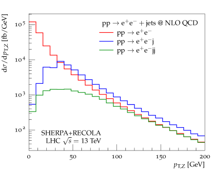
Figure 1: The transverse-momentum distribution of the reconstructed ${\rm Z}$ boson in Drell–Yan plus zero, one and two-jet production at NLO QCD.

Here only the results obtained with Sherpa ​​+Recola are displayed. All results have been cross-checked against Sherpa ​​+O PEN L OOPS , using the identical phase-space points, and no significant deviations have been observed. In fact, for each observable bin the relative difference of the two predictions is well below $10^{-5}$.

3.2.2 ${\rm Z}$-boson pair production

Input parameters:

The set-up employed is the one of Ref. [27] which is, for completeness, repeated in the following. The predictions are for the LHC operating at a centre-of-mass energy of $\sqrt{s}=13\,\text{TeV}$. The NNPDF-2.3QED NLO PDF set [61] with a variable flavour-number scheme and $\alpha_{\text{s}}(M_{\text{Z}})=0.118$ has been used for all computations both at LO and NLO. Furthermore, a fixed factorisation and renormalisation scale at the ${\rm Z}$-boson pole mass $\mu_{\rm R}=\mu_{\rm F}=M_{\rm Z}$ is employed. The strong coupling $\alpha_{\text{s}}$ is extracted from the PDF set at the renormalisation scale $\mu_{\rm R}$, and the electromagnetic coupling $\alpha$ is calculated in the $G_{\mu}$ scheme according to

$$\alpha=\frac{\sqrt{2}}{\pi}G_{\mu}M_{\text{W}}^{2}\left(1-\frac{M_{\text{W}}^{2}}{M_{\text{Z}}^{2}}\right),\qquad\text{with}\qquad G_{\mu}=1.16637\times 10^{-5}\,\text{GeV}^{-2}$$ (5)

denoting the Fermi constant. The on-shell (OS) values for the masses and widths of the massive vector bosons read

$$M_{\text{Z}}^{\text{OS}} =91.1876\,\text{GeV},\qquad \Gamma_{\text{Z}}^{\text{OS}} =2.4952\,\text{GeV},$$

$$M_{\text{W}}^{\text{OS}} =80.385\,\text{GeV},\qquad \Gamma_{\text{W}}^{\text{OS}} =2.085\,\text{GeV}.$$ (6)

They are converted into pole masses and pole widths according to Ref. [67],

$$M_{V}=M_{V}^{\text{OS}}/\sqrt{1+(\Gamma_{V}^{\text{OS}}/M_{V}^{\text{OS}})^{2}},\qquad\Gamma_{V}=\Gamma_{V}^{\text{OS}}/\sqrt{1+(\Gamma_{V}^{\text{OS}}/M_{V}^{\text{OS}})^{2}}\qquad\text{with}\quad V=\text{W},\text{Z}.$$ (7)

Since the top quark and the Higgs boson do not appear as internal resonances, their widths are set equal to zero. The corresponding masses read

$$m_{\text{t}} =173\,\text{GeV},\qquad M_{\rm H} =125\,\text{GeV}.$$ (8)

The masses and widths of all other quarks and leptons have been neglected. As in Ref. [27], the following acceptance cuts are imposed on the charged leptons $\ell^{\pm}$:

$$p_{{\rm T},\ell}>15\,\text{GeV},\qquad|y_{\ell}|<2.5,\qquad\Delta R_{\ell\ell}>0.2.$$ (9)

The jets from real QCD radiation are treated fully inclusively.

NLO QCD validation:

The Sherpa ​​+Recola interface has been cross-checked for this process against the independent private Monte Carlo program that had been used for the computations in Refs. [23, 24, 26, 27].

$\text{p}\text{p}\to\mu^{+}\mu^{-}\text{e}^{+}\text{e}^{-}$	Sherpa ​​+Recola [fb]	private MC+Recola [fb]	std. dev. [$\sigma$]
$\sigma^{\rm LO}$	$11.498(1)$	$11.4964(1)$	$1.6$
$\sigma^{\rm NLO}_{\rm QCD}$	$15.79(1)$	$15.801(2)$	$1.0$

Table 4: Integrated cross sections calculated at $\sqrt{s}=13\,\text{TeV}$ for ${\rm pp}\to\mu^{+}\mu^{-}{\rm e}^{+}{\rm e}^{-}$ at LO and NLO QCD with the Sherpa ​​+Recola interface, compared against the independent private multi-channel Monte Carlo program that was employed for the computations in Ref. [27]. The difference is expressed in standard deviations.

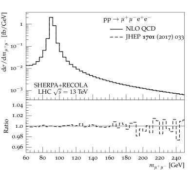
Figure 2: NLO QCD predictions of the di-muon (left) and 4-lepton invariant-mass (right) distributions in $\text{p}\text{p}\to\mu^{+}\mu^{-}\text{e}^{+}\text{e}^{-}$ at $\sqrt{s}=13\,\text{TeV}$. The plots show a direct comparison of Sherpa ​​+Recola to the Monte Carlo program employed in Ref. [27].

The comparison for the total cross section is shown in Table 4. Agreement to four digits is found between the two independent calculations within the statistical uncertainty. Figure 2, shows a comparison at the level of differential distributions between the two Monte Carlo integrations, once for the distribution in the di-muon mass $m_{\mu^{+}\mu^{-}}$ (left plot) and once for the four-lepton invariant mass $m_{4\ell}$ (right plot). The upper panels plot the absolute predictions of the two integrations on top of each other, the differences being almost invisible. The lower panels show the bin-wise ratio between the two calculations. The fluctuations in the four-lepton invariant mass are almost everywhere below 0.5%, from the far off-shell region over the on-shell production threshold at $m_{4\ell}=2M_{\text{Z}}$ up to $1\,\text{TeV}$. A similar pattern is observed for the di-muon mass in the left plot with slightly larger fluctuations.

3.2.3 Higgs production in association with a top-quark pair

Input parameters:

In Ref. [68], a comparison between MadGraph5_aMC@NLO and Sherpa ​​+O PEN L OOPS for various cross sections at LO, NLO QCD, and NLO EW has been presented for the process ${\rm p}{\rm p}\to{\rm t}{\rm\bar{t}}{\rm H}$. In particular, five different cross sections have been reported. The first one is fully inclusive, and no event selections are applied. Two of them are computed when applying a cut on the transverse momentum of the three massive final-state particles at $200\,\text{GeV}$ and $400\,\text{GeV}$, respectively. Furthermore, a cross section with a higher transverse-momentum cut ($500\,\text{GeV}$) on the Higgs boson only is presented and finally the cross section obtained by excluding events with a top quark with absolute rapidity lower than $2.5$. The computations are done for a centre-of-mass energy of $\sqrt{s}=13\,\text{TeV}$ at the LHC. The masses of the involved particles read

$$M_{\rm Z}=91.188\,\text{GeV},\qquad M_{\rm W}=80.385\,\text{GeV},\qquad M_{\rm H}=125\,\text{GeV},\qquad m_{\rm t}=173.3\,\text{GeV},$$ (10)

and the corresponding widths are all set to zero. The bottom quark is considered massless and its PDF contribution is included. The NNPDF-2.3QED PDF set with a variable flavour-number scheme and $\alpha_{\text{s}}(M_{\rm Z})=0.118$ [61, 69, 70] has been used. The renormalisation as well as the factorisation scales are set to a common scale $\hat{H}_{\rm T}/2$, defined as

$$\hat{H}_{\rm T}=\sum_{i}\sqrt{p^{2}_{{\rm T},i}+m^{2}_{i}},$$ (11)

where the index $i$ runs over all the final-state particles. The considered LO production cross section is at the order $\mathcal{O}{\left(\alpha_{\text{s}}^{2}\alpha\right)}$.

NLO QCD validation:

The obtained LO cross sections listed in Table 5 show a generally good agreement.

$\sigma^{\mathrm{LO}}$ [pb]	Sherpa ​​+Recola	MG5_aMC@NLO	Sherpa ​​+O PEN L OOPS
inclusive	$3.612(4)\cdot 10^{-1}$	$3.617\cdot 10^{-1}$	$3.617\cdot 10^{-1}$
$p_{{\rm T},{\rm t/\bar{t}/H}}>200\,\text{GeV}$	$1.338(2)\cdot 10^{-2}$	$1.338\cdot 10^{-2}$	$1.338\cdot 10^{-2}$
$p_{{\rm T},{\rm t/\bar{t}/H}}>400\,\text{GeV}$	$4.001(4)\cdot 10^{-4}$	$3.977\cdot 10^{-4}$	$3.995\cdot 10^{-4}$
$p_{{\rm T},{\rm H}}>500\,\text{GeV}$	$2.015(3)\cdot 10^{-3}$	$2.013\cdot 10^{-3}$	$2.014\cdot 10^{-3}$
$\left|y_{\rm t}\right|>2.5$	$5.017(5)\cdot 10^{-3}$	$4.961\cdot 10^{-3}$	$5.006\cdot 10^{-3}$

Table 5: Integrated cross sections for ${\rm p}{\rm p}\to{\rm t}{\rm\bar{t}}{\rm H}$ at LO for a centre-of-mass energy of $\sqrt{s}=13\,\text{TeV}$ calculated with Sherpa ​​+Recola, MadGraph5_aMC@NLO, and Sherpa ​​+O PEN L OOPS for the set-up of Ref. [68]. The cross sections are expressed in pb. The integration errors of the last digits are given in parentheses for the Sherpa ​​+Recola predictions.

The corresponding NLO QCD predictions of order $\mathcal{O}{\left(\alpha_{\text{s}}^{3}\alpha\right)}$ are reproduced in Table 6.

	Sherpa ​​+Recola		MG5_aMC@NLO	Sherpa ​​+O PEN L OOPS
	$\sigma^{\mathrm{NLO}}_{\rm QCD}$ [pb]	$\delta_{\rm QCD}[\%]$	$\delta_{\rm QCD}[\%]$	$\delta_{\rm QCD}[\%]$
inclusive	$4.6407(9)\cdot 10^{-1}$	$28.5(2)$	$28.9$	$28.3$
$p_{{\rm T},{\rm t/\bar{t}/H}}>200\,\text{GeV}$	$1.630(2)\cdot 10^{-2}$	$21.9(2)$	$23.4$	$22.5$
$p_{{\rm T},{\rm t/\bar{t}/H}}>400\,\text{GeV}$	$4.289(5)\cdot 10^{-4}$	$7.2(2)$	$9.6$	$10.4$
$p_{{\rm T},{\rm H}}>500\,\text{GeV}$	$2.747(3)\cdot 10^{-3}$	$36.3(2)$	$37.8$	3$7.3$
$\left|y_{\rm t}\right|>2.5$	$6.840(7)\cdot 10^{-3}$	$36.3(2)$	$37.5$	$36.9$

Table 6: Integrated cross sections for ${\rm p}{\rm p}\to{\rm t}{\rm\bar{t}}{\rm H}$ at NLO QCD for a centre-of-mass energy $\sqrt{s}=13\,\text{TeV}$ calculated with Sherpa ​​+Recola, MadGraph5_aMC@NLO, and Sherpa ​​+O PEN L OOPS for the set-up of Ref. [68]. The cross sections are expressed in pb while the relative corrections are expressed in per cent. The integration errors of the last digits are given in parentheses for the Sherpa ​​+Recola predictions.

The agreement is reasonable but a definite statement is not possible as the predictions made by MadGraph5_aMC@NLO and Sherpa ​​+O PEN L OOPS do not have statistical errors. In addition we have cross-checked the fully inclusive set-up at the level of distributions against the public Sherpa ​​+O PEN L OOPS implementation, finding perfect agreement in each bin. The distributions for Sherpa ​​+Recola are shown in the plots of Fig. 3.

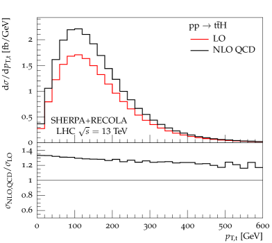
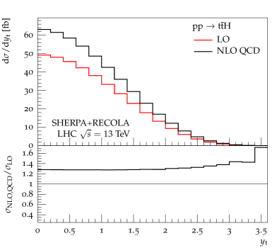
Figure 3: Differential distributions at a centre-of-mass energy $\sqrt{s}=13\,\text{TeV}$ for ${\rm pp}\to{\rm t\bar{t}H}$ at the LHC in a fully inclusive set-up: transverse momentum distribution of the top quark (left) and rapidity distribution of the top quark (right).

3.2.4 Higgs-boson production in association with a ${\rm Z}$ boson

As last example, Higgs-boson production in association with an on-shell ${\rm Z}$ boson is considered. This channel is particularly interesting, as it receives sizeable contributions from the loop-induced $\text{g}\text{g}\to\text{H}\text{Z}$ channel.

Input parameters:

The set-up used is similar to the one of the Drell–Yan example described in Section 3.2.1. However, here we use the partonic centre-of-mass energy $\sqrt{\hat{s}}$ as the renormalisation and factorisation scale. For the Higgs boson we assume the decay into a pair of bottom quarks, that is, however, fully factorised from the production process. The mass of the bottom quark is thereby taken to be $m_{\text{b}}=4.8\,\text{GeV}$.

NLO QCD validation:

The LO contribution appears at order $\mathcal{O}{\left(\alpha^{2}\right)}$ for the quark-initiated channel, hence the NLO QCD cross section is of order $\mathcal{O}{\left(\alpha_{\text{s}}\alpha^{2}\right)}$. The loop-induced $\text{g}\text{g}\to\text{H}\text{Z}$ process contributes at order $\mathcal{O}{\left(\alpha_{\text{s}}^{2}\alpha^{2}\right)}$ but is enhanced by the gluon PDF. The comparison for the total cross sections calculated with Sherpa ​​+Recola and Sherpa ​​+O PEN L OOPS can be found in Table 7. Again, perfect agreement is found, originating from the fact that both cross sections have been evaluated using the same phase-space points such that there is no statistical difference, and the deviations per point are below $10^{-9}$ (cf. Section 3.1).

$\sigma^{\mathrm{NLO}}_{\mathrm{QCD}}$	Sherpa ​​+Recola [pb]	Sherpa ​​+O PEN L OOPS [pb]
$\text{q}\bar{}\text{q}\to\text{H}\text{Z}$	$0.41012(9)$	$0.41012(9)$
$\text{g}\text{g}\to\text{H}\text{Z}$	$0.029482(2)$	$0.029482(2)$

Table 7: Total cross sections calculated for ${\rm pp}\to{\rm H}{\rm Z}$ at NLO QCD with the Sherpa ​​+Recola interface, compared against Sherpa ​​+O PEN L OOPS .

In Fig. 4 the transverse-momentum distribution of the reconstructed Higgs boson is presented, where the quark- and the gluon-initiated channels are shown separately. Though much smaller than the quark-induced contribution, the loop-induced gluon-initiated channel still contributes around $10\%$ to the total cross section for Higgs transverse momenta in the range $100$–$200\,\text{GeV}$. This nicely illustrates the importance of precise predictions of this phenomenologically important Higgs-production process. Considering even larger values of $p_{\text{T,H}}$ the gluon contribution falls off more steeply, due to the different slope of the quark and gluon parton-density functions. Let us note that the results for the differential distributions have explicitly been checked against Sherpa ​​+O PEN L OOPS , and using identical phase-space points perfect agreement has been found.

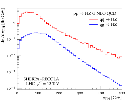
Figure 4: The transverse-momentum distribution of the reconstructed $\text{b}\bar{}\text{b}$-decayed H boson in the $\text{p}\text{p}\to{\rm HZ}$ process at NLO QCD.

3.3 Matching to parton shower

To illustrate and validate the use of virtual QCD matrix elements from Recola for full particle-level simulations, a state-of-the-art QCD calculation is presented where NLO QCD matrix elements of varying final-state parton multiplicity get matched to the QCD parton shower of Sherpa [37] and subsequently hadronised. In particular, the Drell–Yan process is investigated, i.e. $\text{p}\text{p}\to\gamma^{*}/{\rm Z}^{*}\to\text{e}^{+}\text{e}^{-}/\mu^{+}\mu^{-}$, in association with jets in the MEPS@NLO scheme [40]. To this end, NLO QCD matrix elements are considered for up to two additional jets and the tree-level contribution for three final-state partons. The phase-space slicing parameter of the merging scheme is set to $Q_{\rm{cut}}=20\,\text{GeV}$. The NNPDF-3.0 NNLO PDF set is employed with $\alpha_{\text{s}}(M_{\rm Z})=0.118$ and five active flavours. For the electromagnetic coupling constant $\alpha$, the $\alpha(M_{\text{Z}})$ scheme is used with a numerical value of $\alpha(M_{\text{Z}})=0.007764$. In the MEPS@NLO approach the renormalisation and factorisation scales are chosen dynamically, based on the determination of an event-wise $2\to 2$ core process and an associated sequence of nodal splitting scales, obtained through a clustering of the matrix-element partons that effectively inverts the Sherpa parton shower [38, 39, 71]. To estimate the scale uncertainties, a 7-point scale variation is considered for $\mu_{\rm{R}}$ and $\mu_{\rm{F}}$, computed by reweighting the central prediction  [43]. Both scales are varied independently by factors of $1/2$ and $2$, thereby omitting the variations with ratios of 4 between the two scales. The corresponding uncertainty is then taken as the envelope of all variations considered.

The Sherpa ​​+Recola MEPS@NLO results are compared against corresponding data from the ATLAS and CMS experiments taken at $\sqrt{s}=7\,\text{TeV}$. The CMS analysis of jet-associated Drell–Yan production presented in Ref. [72] assumes pairs of electrons or muons with an invariant mass between $71$ and $111\,\text{GeV}$. Furthermore, the leptons have to exhibit a transverse momentum of $p_{{\rm T},{\ell}}>20\,\text{GeV}$. Jets are reconstructed according to the anti-$k_{\rm T}$ algorithm with a radius parameter of $R=0.5$. A transverse-momentum threshold for jets of $p_{{\rm T},{\rm j}}>30\,\text{GeV}$ is assumed, and only jets with $|\eta_{\rm j}|<2.4$ are considered. In addition, all jets are required to be separated from the leptons by $\Delta R_{{\rm j}{\ell}}\geq 0.5$. Similarly, in the ATLAS analysis presented in Ref. [73] electron and muon pairs within a mass range of $66\,\text{GeV}\leq m_{\ell\ell}\leq 116\,\text{GeV}$ are selected and the leptons must have $p_{{\rm T},{\ell}}>20\,\text{GeV}$. Anti-$k_{\rm T}$ jets with a radius parameter of $R=0.4$, $p_{{\rm T},{\rm j}}>30\,\text{GeV}$ and $|y_{\rm j}|<4.4$ are considered. Each jet candidate needs to be separated from the reconstructed leptons by $\Delta R_{{\rm j}{\ell}}\geq 0.5$. For the study presented here, the public Rivet implementations of the two analyses were used, allowing for a direct comparison to particle-level results. Further details on the selections can be found in the respective publications.

Figures 5 and 6 provide examples for the comparison of particle-level MEPS@NLO simulations based on Sherpa ​​+Recola against data. In the left panel of Fig. 5 the inclusive transverse-momentum distribution of the reconstructed ${\rm Z}$ bosons is compared to the ATLAS data from Ref. [73]. The inclusion of the ${\rm Z}+{\text{j}}$ and ${\rm Z}+{\text{j}\text{j}}$ matrix elements at NLO QCD accuracy provides a good description of events with sizeable recoil of the Drell–Yan pair. The parton-shower component, on the other hand, dominates the low-$p_{{\rm T},{\rm Z}}$ region. Notably, the theoretical scale uncertainties are of order $\pm 20\%$ and well overlap with the experimental uncertainty band, indicated in yellow. The right panel of Fig. 5 presents the comparison of the jet-multiplicity distribution against the data from CMS [72]. By construction of the MEPS@NLO algorithm, in the given set-up, the first two bins have NLO QCD accuracy, while the third has LO QCD precision. All higher jet multiplicities solely originate from the QCD parton-shower component. The central theoretical predictions agree well with the data though there is a tendency to overestimate higher jet counts. However, taking into account theoretical and experimental uncertainties, simulation and data agree well.

Finally, Fig. 6 presents the transverse-momentum distributions of the two leading jets. The set-up provides NLO QCD accuracy for both observables. The predictions are compared to the respective LHC data from CMS [72]. Very good agreement of data and theoretical prediction is found. For the latter the theoretical uncertainty estimates from variations around the central scale choice increase for larger jet transverse momenta, exceeding the $\pm 20\%$ range seen in the more inclusive boson transverse momentum distribution.

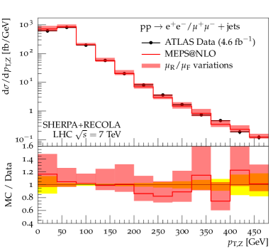
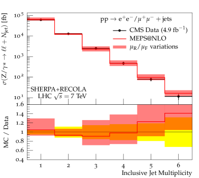
Figure 5: The left-hand figure compares the MEPS@NLO predictions based on Sherpa ​​+Recola for the transverse-momentum distribution of the reconstructed ${\rm Z}$ boson compared to $\sqrt{s}=7\,\text{TeV}$ LHC data from ATLAS [73]. The right-hand figure shows the inclusive jet multiplicity in comparison to $\sqrt{s}=7\,\text{TeV}$ CMS data [72]. The theoretical-uncertainty band is obtained through 7-point scale variations of $\mu_{\rm R}$ and $\mu_{\rm F}$. The yellow bands in the lower panels indicate the measurements combined statistical and systematic uncertainty.

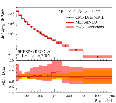
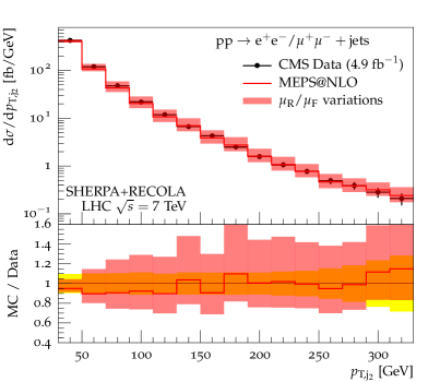
Figure 6: Transverse-momentum distribution of the first (left panel) and second (right panel) hardest jet for Drell–Yan production at the LHC with $\sqrt{s}=7\,\text{TeV}$. The MEPS@NLO predictions from Sherpa ​​+Recola are compared to CMS data from Ref. [72] (uncertainty bands as in Fig. 5).

The results for the jet-associated Drell–Yan process based on Sherpa ​​+Recola presented here confirm related comparisons of simulations based on NLO QCD matrix elements matched with QCD parton showers with data, see e.g. Refs. [74, 75]. This nicely illustrates the usability of the Recola loop-amplitude generator in these highly non-trivial multi-scale calculations. To this end, the same set-up has been explicitly compared, but using the O PEN L OOPS generator for the one-loop amplitudes. For all distributions considered, embracing many more than presented here, full agreement between Sherpa ​​+Recola and Sherpa ​​+O PEN L OOPS has been observed. Besides, in this “real-life” application no significant run-time differences have been observed. However, when using Recola instead of O PEN L OOPS the allocated memory increases by about $50\%$ for the process set-up considered.

4 NLO EW validation and combined predictions

To illustrate the capabilities of the combination of Sherpa with Recola, three processes have been computed at both NLO QCD and EW accuracy. These comprise off-shell vector-boson production in association with jets, the production of two off-shell ${\rm Z}$ bosons, and the on-shell production of a top-quark pair in association with a Higgs boson. These three channels represent phenomenologically very important LHC processes. Furthermore, they are highly non-trivial, and each process features different technical challenges regarding their evaluation to NLO QCD and EW accuracy, thus demonstrating the generality of our implementation. Since up to now there is no public code that allows the computation of arbitrary processes at NLO EW accuracy, the number of processes that have been checked is smaller than for QCD.

For each process, a short introduction is given followed by the description of the calculational set-up and the actual NLO EW validation. Finally, the cross sections and differential distributions for combined NLO QCD and EW accuracy are presented. The cross sections including NLO QCD or EW corrections read

$$\sigma^{\mathrm{NLO}}_{\mathrm{QCD}}=\sigma^{\mathrm{LO}}+\delta\sigma^{\mathrm{NLO}}_{\mathrm{QCD}}\qquad\text{and}\qquad\sigma^{\mathrm{NLO}}_{\mathrm{EW}}=\sigma^{\mathrm{LO}}+\delta\sigma^{\mathrm{NLO}}_{\mathrm{EW}},$$ (12)

respectively. The additive combination of the two types of corrections is straight-forward,

$$\sigma^{\mathrm{NLO}}_{\mathrm{QCD+EW}}=\sigma^{\mathrm{LO}}+\delta\sigma^{\mathrm{NLO}}_{\mathrm{QCD}}+\delta\sigma^{\mathrm{NLO}}_{\mathrm{EW}},$$ (13)

while a multiplicative combination can be defined as

$$\sigma^{\mathrm{NLO}}_{\mathrm{QCD}\times\mathrm{EW}}=\sigma^{\mathrm{NLO}}_{\mathrm{QCD}}\left(1+\frac{\delta\sigma^{\mathrm{NLO}}_{\mathrm{EW}}}{\sigma^{\mathrm{LO}}}\right)=\sigma^{\mathrm{NLO}}_{\mathrm{EW}}\left(1+\frac{\delta\sigma^{\mathrm{NLO}}_{\mathrm{QCD}}}{\sigma^{\mathrm{LO}}}\right).$$ (14)

The difference between these two ways of combining NLO QCD and EW corrections provides an estimate of the missing higher orders resulting from mixed QCD–EW contributions. The NLO QCD$\times$EW combination can be understood as an improved prediction when the typical scales of the QCD and EW corrections are well separated.

4.1 Vector-boson production in association with jets

As a first process, the production of a vector boson plus jets is considered. This process has already been computed for the LHC running at a centre-of-mass energy of $13\,\text{TeV}$ for both on- and off-shell vector bosons at NLO QCD and EW [22, 29, 30], and therefore allows a comparison to existing results. From the technical point of view, the process is a mixture of QCD and EW contributions. In particular, for vector-boson production in association with more than one jet at NLO EW, interferences appear between QCD and EW production channels. This makes vector-boson-plus-jets production a good testing ground of the interface, although it is also an important process in its own right.

Input parameters:

The input parameters for this process class are taken from Ref. [76] to allow a tuned comparison. For completeness, these parameters as well as the analysis cuts are detailed here. The renormalisation and factorisation scale for off-shell W-boson production is $\hat{H}^{\prime}_{{\rm T},{\rm W}}/2$, defined via

$$\hat{H}^{\prime}_{{\rm T},{\rm W}}=\sum_{i=\text{q},\text{g}}p_{{\rm T},i}+p_{{\rm T},\gamma}+\sqrt{p_{{\rm T},\ell\nu}^{2}+m_{\ell\nu}^{2}}.$$ (15)

The scales used in off-shell ${\rm Z}$-boson production, $\hat{H}^{\prime}_{{\rm T},{\rm Z}}/2$, are similarly given by

$$\hat{H}^{\prime}_{{\rm T},{\rm Z}}=\sum_{i=\text{q},\text{g}}p_{{\rm T},i}+p_{{\rm T},\gamma}+\sqrt{p_{{\rm T},\ell\ell}^{2}+m_{\ell\ell}^{2}}.$$ (16)

For on-shell weak-boson production, a slightly different scale, $\hat{H}_{{\rm T}}/2$, is used, defined via

$$\hat{H}_{\rm T}=\sum_{i=\text{q},\text{g}}p_{{\rm T},i}+p_{{\rm T},\gamma}+\sqrt{p_{{\rm T},{V}}^{2}+M_{V}^{2}},$$ (17)

where ${V}$=${\rm W},{\rm Z}$ for ${\rm W}$+jets and ${\rm Z}$+jets production, respectively. No scale variations have been considered for this validation, although a variation of a factor of $1/2$ and $2$ on the central scale was considered in the original article.

For on-shell vector-boson production, the bosons are decayed to leptons in a factorised approach, thereby preserving the spin correlations [59]. For ${\rm W}$-boson production, the leptonic decay channels ${\rm W}^{\pm}\to{\rm e}^{\pm(}\overline{\nu}^{)}_{e}$ and ${\rm W}^{\pm}\to\mu^{\pm(}\overline{\nu}^{)}_{\mu}$ are considered. Similarly, for ${\rm Z}$-boson production, the allowed leptonic decay channels are ${\rm Z}\to{\rm e}^{+}{\rm e}^{-}$ and ${\rm Z}\to\mu^{+}\mu^{-}$. For all processes in this section, the masses for the ${\rm Z}$ boson, ${\rm W^{\pm}}$ bosons, ${\rm H}$ boson and top quark read

$$M_{\rm Z}=91.1876\,\text{GeV},\qquad M_{\rm W}=80.385\,\text{GeV},\qquad M_{\rm H}=126\,\text{GeV},\qquad m_{\rm t}=173.2\,\text{GeV}.$$ (18)

The Fermi constant is taken to be $G_{\mu}=1.1667\times 10^{-5}\,\text{GeV}^{-2}$, and the $G_{\mu}$ scheme is used to consistently define the EW parameters. The NNPDF-2.3QED NLO PDF set with a variable flavour-number scheme, QED corrections and $\alpha_{s}(M_{\rm Z})=0.118$ [61, 69, 70] has been used for both LO and NLO calculations.

For on-shell vector-boson production, the widths of the external bosons are set to zero in general. An exception to this rule is in the QCD–EW interference term introduced in the EW real-subtracted contribution which includes electroweakly produced jets leading to a poorly converging phase-space integration. Because this enters only as an interference term, it does not give rise to a true resonance and maintaining a width of zero is theoretically acceptable. Following Ref. [29], a small, artificial width for the ${\rm W}$ and ${\rm Z}$ bosons is introduced in this case in order to control the phase-space integration. In this publication we use $0.3\,\text{GeV}$.

For the off-shell vector-boson production processes, physical values of the vector-boson widths are used, as well as for other unstable particles such as the Higgs boson and the top quark,

$$\Gamma_{\rm Z}=2.4955\,\text{GeV},\qquad\Gamma_{\rm W}=2.0897\,\text{GeV},\qquad\Gamma_{\rm H}=4.07\,\text{MeV},\qquad\Gamma_{\rm t}=1.339\,\text{GeV}.$$ (19)

Furthermore, the complex-mass scheme is employed for the unstable particles in this case, and a unit CKM matrix is assumed.

Photons within a rapidity–azimuthal-angle distance of $R_{\gamma\text{q}/\ell}=0.1$ from a quark or lepton are recombined with a simple cone-like algorithm with the closest charged particle. Jets are defined with the anti-$k_{\mathrm{T}}$ algorithm using $R=0.4$ and

$$p_{{\rm T},{\rm j}}>30\,\text{GeV},\qquad|\eta_{\rm j}|<4.5\,.$$ (20)

Any jet with more than $50\%$ of its energy originating from a photonic contribution is removed from the jet list.

For the cross section validation for on-shell ${\rm W+j}$ production, two phase-space regions, other than the inclusive cross section subject to the cuts (20), are considered, defined by the additional cuts

$$p_{{\rm T},{\rm W}}>1\,\text{TeV},\qquad p_{{\rm T},{\rm j}}>1\,\text{TeV}.$$ (21)

Distributions have been analysed with Rivet following Ref. [30] and using the cuts shown in Table 8.

cut variable	$\ell^{\pm(}\overline{\nu}^{)}$	$\ell^{+}\ell^{-}$
$p_{\rm{T},\ell^{\pm}}/\,\text{GeV}>$	$25$	$25$
$E_{{\rm T}}^{\rm miss}/\,\text{GeV}>$	$25$	–
$m_{\rm T}^{\rm W}/\,\text{GeV}>$	$40$	–
$|\eta_{\ell^{\pm}}|<$	$2.5$	$2.5$
$\Delta R_{\ell^{\pm}{\rm j}}>$	$0.5$	$0.5$
$\Delta R_{\ell^{+}\ell^{-}}>$	–	$0.2$
$m_{\ell^{+}\ell^{-}}/\,\text{GeV}\in$	–	$[66,116]$

Table 8: Event selections used for the Rivet analyses for the ${V+jets}$ distributions, where $m_{\rm T}^{\rm W}=\sqrt{2p_{{\rm T},{\ell}}p_{{\rm T},\nu}(1-\cos\Delta\Phi_{{\ell}\nu})}$.

NLO EW validation:

Next, we present the validation of the Sherpa ​​+Recola interface against published cross sections obtained with Sherpa ​​+O PEN L OOPS  [29, 76, 30]. First, on-shell ${\rm W+j}$ production at a centre-of-mass energy of $13\,\text{TeV}$ at the LHC is considered.

$\sigma^{\mathrm{NLO}}_{\mathrm{QCD+EW}}$	Sherpa ​​+O PEN L OOPS [pb]	Sherpa ​​+Recola [pb]	$\delta[\%$]
inclusive	$15621$	$15592(30)$	$0.19$
$p_{{\rm T},{\rm W}}>1\,\text{TeV}$	$0.040$	$0.0400(2)$	$0$
$p_{{\rm T},{\rm j}}>1\,\text{TeV}$	$0.195$	$0.194(1)$	$0.51$

Table 9: Cross sections at $13\,\text{TeV}$ for $\text{p}\text{p}\to{\rm W}^{\pm}{\rm j}$ at the LHC at NLO QCD and EW with Sherpa ​​+Recola, compared to published results with Sherpa ​​+O PEN L OOPS [29, 30, 76].

Table 9 shows the relative difference between total cross-section calculations, with different phase-space cuts, for the Sherpa ​​+Recola interface against the published numbers from Sherpa ​​+O PEN L OOPS . The errors quoted on the Sherpa ​​+Recola cross sections are statistical in origin. While for the Sherpa ​​+O PEN L OOPS results scale uncertainties were presented, the comparably negligible statistical uncertainties were not listed. However, for the validation of the codes, it is necessary to demonstrate close statistical agreement with the published numbers for the central scale choice. Taking the statistical errors of Sherpa ​​+Recola as benchmark, good agreement between the two calculations for the NLO QCD and EW total cross sections is observed in all cases.

Besides the integrated cross sections, Ref. [29] also provides distributions, which can be used for a more qualitative validation over a large phase space. Figure 7 displays the $p_{\rm T}$ distribution of the hardest jet in on-shell $\text{W}^{+}+\text{j}$ production. The left-hand side of Fig. 7 shows the inclusive prediction, and the right-hand side the effect of a phase-space cut $\Delta\Phi({\rm j},{\rm j})<3\pi/4$. This effect is very large, in line with the findings in Ref. [29]. The Sudakov behaviour in the large-$p_{\rm T}$ region is clearly recovered once this $\Delta\Phi({\rm j},{\rm j})$ cut is included, because it removes the contributions from dijet-like structures with a soft W boson emitted. At NLO EW, these types of contributions can be better viewed as a real EW correction to dijet production.

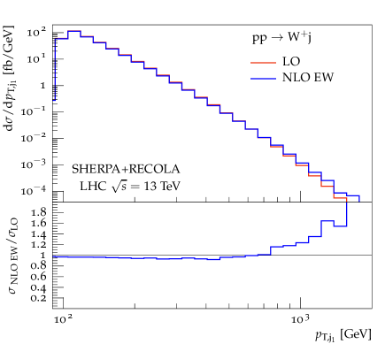
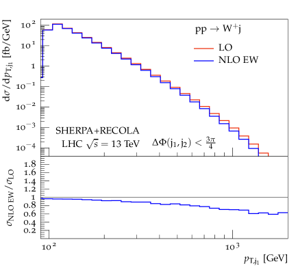
Figure 7: Differential distributions at $13\,\text{TeV}$ for $\text{p}\text{p}\to{\rm W}^{+}{\rm j}$ at the LHC, both at LO and NLO EW. The left-hand figure shows the leading-jet $p_{\rm T}$ with minimal cuts and the right-hand plot the leading-jet $p_{\rm T}$ with an additional cut $\Delta\Phi({\rm j},{\rm j})<3\pi/4$. The lower panels display the ratio of the NLO EW calculation to the corresponding LO result.

Secondly, ${\rm Z}$+jets production is considered. Distributions have been published for off-shell ${\rm Z}$+jets processes in Ref. [30]. Although this is not such a rigorous validation as the total cross section or phase-space point comparisons for other processes, it allows a qualitative assessment of the agreement between the calculations across a large phase space. From the wide range of distributions presented in Ref. [30], we select here the distributions in the transverse momenta of the leading lepton, $p_{{\rm T},{\ell}_{1}}$, and leading jet, $p_{{\rm T},{\rm j}_{1}}$, (according to $p_{{\rm T}}$ ordering) (Fig. 8). The $\text{p}\text{p}\to\ell^{+}\ell^{-}{\rm jj}$ process provides a particularly good test of the Sherpa ​​+Recola interface, because it includes interference terms between EW and QCD produced jets contributing at NLO EW. This makes the process a lot more challenging than the $\ell^{+}\ell^{-}{\rm j}$ or $\ell\nu{\rm j}$ final state. For both plots in Fig. 8, the behaviour across the full $p_{\rm T}$ range is in agreement with the observations in Ref. [30].

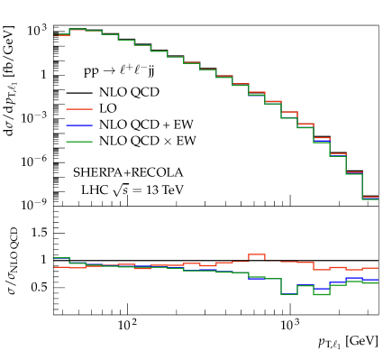
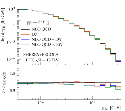
Figure 8: Differential distributions at $13\,\text{TeV}$ for $\text{p}\text{p}\to\ell^{+}\ell^{-}{\rm j}{\rm j}$ at the LHC. The left-hand plot shows the $p_{\rm T}$ of the hardest lepton and the right-hand plot the $p_{\rm T}$ of the hardest jet. The LO and NLO QCD distributions are plotted along with both the additive (NLO QCD + EW) and multiplicative (NLO QCD $\times$ EW) prescriptions for combining the NLO corrections. The ratio of the distributions with respect to NLO QCD is presented in the lower panels.

Combined predictions:

Table 10 presents combined predictions for NLO QCD and EW corrections to the integrated cross sections for ${\rm Z}/\ell^{+}\ell^{-}+{\rm jets}$ processes. These cross sections include all of the cuts from the analyses, and correspond to the distributions presented in this section. The on-shell calculation of $\text{Z}+{\rm jets}$ includes the branching ratios to $\text{e}^{+}\text{e}^{-}/\mu^{+}\mu^{-}$. The large NLO corrections are dominated, in all cases, by the NLO QCD contribution.

inclusive	$\sigma^{\mathrm{LO}}$ [pb]	$\sigma^{\mathrm{NLO}}_{\mathrm{QCD}+\mathrm{EW}}$ [pb]	$\delta^{\mathrm{NLO}}_{\mathrm{QCD}+\mathrm{EW}}$ [%]	$\sigma^{\mathrm{NLO}}_{\mathrm{QCD}\times\mathrm{EW}}$ [pb]	$\delta^{\mathrm{NLO}}_{\mathrm{QCD}\times\mathrm{EW}}$ [%]
$\text{p}\text{p}\to\text{Z}{\rm j}$	$1.97\cdot 10^{2}$	$2.68\cdot 10^{2}$	$36.2$	$2.72\cdot 10^{2}$	$38.3$
$\text{p}\text{p}\to\text{Z}{\rm jj}$	$6.66\cdot 10^{1}$	$7.70\cdot 10^{1}$	$15.6$	$7.68\cdot 10^{1}$	$15.3$
$\text{p}\text{p}\to\ell^{+}\ell^{-}{\rm j}$	$1.93\cdot 10^{2}$	$2.34\cdot 10^{2}$	$21.6$	$2.31\cdot 10^{2}$	$19.7$
$\text{p}\text{p}\to\ell^{+}\ell^{-}{\rm jj}$	$5.53\cdot 10^{1}$	$6.93\cdot 10^{1}$	$0.04$	$6.88\cdot 10^{1}$	$0.03$

Table 10: Integrated cross sections for ${\rm p}{\rm p}\to{\rm Z+jets}$ for a centre-of-mass energy of $\sqrt{s}=13\,\text{TeV}$ calculated with Sherpa ​​+Recola. The cross sections at LO as well as for the additive and multiplicative combinations of NLO QCD and EW corrections are given. The cross sections are expressed in pb while the relative corrections are given in percent.

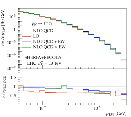
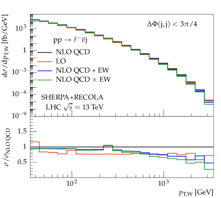
Figure 9: Differential distributions at $13\,\text{TeV}$ for off-shell ${\rm W}+{\rm j}$ production at the LHC. The left-hand plot shows the $p_{\rm T}$ of the reconstructed ${\rm W}$ boson with minimal cuts and the right-hand plot the result with a cut of $\Delta\Phi({\rm j},{\rm j})<3\pi/4$.

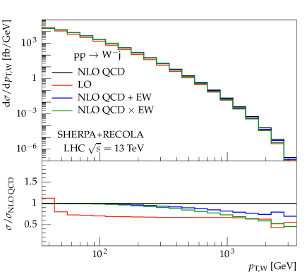
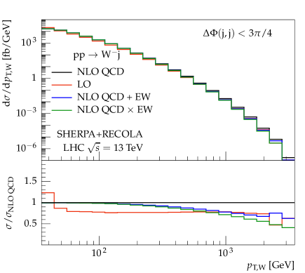
Figure 10: Differential distributions at $13\,\text{TeV}$ for on-shell ${\rm W}+{\rm j}$ production at the LHC. The left-hand plot shows the $p_{\rm T}$ of the ${\rm W}$ boson with minimal cuts and the right-hand plot the result with a cut of $\Delta\Phi({\rm j},{\rm j})<3\pi/4$, as in Fig. 9.

Beginning again with ${\rm W+j}$ production, distributions at a centre-of-mass energy of $13\,\text{TeV}$ at the LHC are presented for both on-shell and off-shell ${\rm W+j}$ production. Figure 9 shows the transverse momentum $p_{\rm T,\text{W}}$ of the reconstructed W boson for both additive and multiplicative combination of NLO QCD and EW effects. The prescription used to combine the NLO corrections clearly has a large effect in the high-$p_{\rm T}$ region of the plot, which is indicative of large higher-order corrections. The right-hand plot shows the effect of imposing a cut $\Delta\Phi({\rm j},{\rm j})<3\pi/4$ on the two jets in the NLO case. This removes the contribution from the production of two hard jets and a soft ${\rm W}$ boson. At NLO EW, such cuts are useful in order to differentiate processes which should more correctly be considered as an EW real correction to dijet production.

Similarly, Fig. 10 shows the distributions for on-shell ${\rm W}+\text{j}$ production. The decays to leptons are treated in a factorised approach, and the NLO QCD and NLO EW corrections are applied only to the on-shell ${\rm W+j}$ final state. The NLO QCD and NLO EW corrections show very similar behaviour, whether on-shell or off-shell ${\rm W}$-boson production is considered.

Results are also presented for ${\rm Z}$+jets production in Figs. 11 and 12, but this time considering both the $1$-jet and $2$-jet channels as well as the on-shell vs. off-shell effects. The off-shell process naturally includes the effects from $\gamma^{*}\to\ell^{+}\ell^{-}$ interference. As was mentioned in the validation section for this process, the ${\rm Z}+2\,$jets final state introduces interference terms between NLO QCD and NLO EW, which are taken into account automatically. These plots display the (reconstructed) $p_{\rm T}$ of the ${\rm Z}$ boson. The distribution for $\ell^{+}\ell^{-}{\rm jj}$ shown in Fig. 12, was also presented in Ref. [30], and can therefore be additionally viewed as a further validation of the Sherpa ​​+Recola interface.

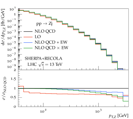
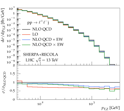
Figure 11: Differential distributions at $13\,\text{TeV}$ for ${\rm Z}+{\rm j}$ production at the LHC. The left-hand plot shows the $p_{\rm T}$ of the ${\rm Z}$ boson for on-shell ${\rm Z}$ production and the right-hand plot the same observable for the reconstructed ${\rm Z}$ boson for off-shell ${\rm Z}$ production. The lower panels display the ratio of the distributions to the NLO QCD result.

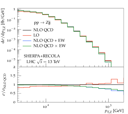
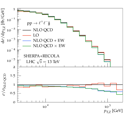
Figure 12: Differential distributions at $13\,\text{TeV}$ for ${\rm Z}+{\rm jj}$ production at the LHC. The left-hand plot shows the $p_{\rm T}$ of the reconstructed ${\rm Z}$ boson for on-shell ${\rm Z}$ production and the right-hand plot the same observable for off-shell ${\rm Z}$ production. The lower panels display the ratio of the distributions to the NLO QCD result.

Figure 11 presents the ${\rm Z}$-boson $p_{\rm T}$ in ${\rm Z+j}$ production at a $13\,\text{TeV}$ LHC. Here, there is a larger impact from the NLO EW corrections in the low-$p_{\rm T}$ region for $\ell^{+}\ell^{-}{\rm j}$ production than for on-shell ${\rm Z+j}$ production. This effect is smaller for the $\ell^{+}\ell^{-}{\rm jj}$ final state shown in Fig. 12, where little difference is observed between on-shell and off-shell ${\rm Z}$-boson production across the entire phase space. In all cases, the Sudakov behaviour in the large-$p_{\rm T}$ region is clearly observed. Also, the NLO QCD + EW and NLO QCD $\times$ EW curves for ${\rm Z+jj}$ in Fig. 12 show a very good agreement with each other, indicating that the higher-order corrections in this case are a lot smaller than for the distributions of ${\rm Z+j}$ production, where a large difference is observed in the high-$p_{\rm T}$ Sudakov region. It is reassuring that these differences are largely removed for both the on-shell and off-shell ${\rm Z}$+jets processes once higher jet multiplicities are included. This implies that a merged NLO QCD and EW sample would give an accurate picture of both NLO QCD and NLO EW corrections to this process.

4.2 ${\rm Z}$-boson pair production

As second process we consider the production of two off-shell Z bosons with subsequent decays into pairs of different-flavour charged leptons. At leading order (LO), this is a purely EW process implying that interferences in different orders of the strong and EW coupling first occur at NNLO. As a consequence, the NLO QCD corrections at ${\cal{O}}(\alpha_{\text{s}}$) and the NLO EW corrections at ${\cal{O}}(\alpha)$ may be computed independently. The NLO QCD corrections are known [77, 78, 79, 80], and the complete NLO EW computations have recently been published [24, 27].

Input parameters:

We use the same set-up as for the QCD validation of Z-boson pair production in Section 3.2. In addition, real photons from QED bremsstrahlung and charged leptons are recombined to dressed leptons if their separation in the rapidity–azimuthal-angle plane fulfils $\Delta R_{\ell\gamma}<0.2$, following the prescription of Ref. [27]. In contrast to Ref. [27], we refrain from including photon-induced contributions.

NLO EW validation:

In Table 11, a comparison of the NLO EW total cross section is shown once obtained from Sherpa ​​+Recola and once by combining Recola with an independent private multi-channel Monte Carlo integrator, i.e. with the results from Ref. [27]. Perfect agreement is found between the two calculations within the statistical uncertainty at (sub-)permille level.

$\text{p}\text{p}\to\mu^{+}\mu^{-}\text{e}^{+}\text{e}^{-}$	Sherpa ​​+Recola [fb]	private MC+Recola [fb]	std. dev. [$\sigma$]
$\sigma^{\rm LO}$	$11.498(1)$	$11.4964(1)$	$1.6$
$\sigma^{\rm NLO}_{\rm EW}$	$10.890(1)$	$10.8888(2)$	$1.2$

Table 11: Total cross sections calculated for ${\rm pp}\to\mu^{+}\mu^{-}{\rm e}^{+}{\rm e}^{-}$ at LO and NLO EW with the Sherpa ​​+Recola interface, compared against the benchmark numbers from Ref. [27]. The difference is expressed in standard deviations.

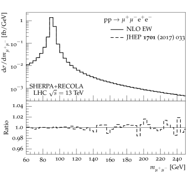
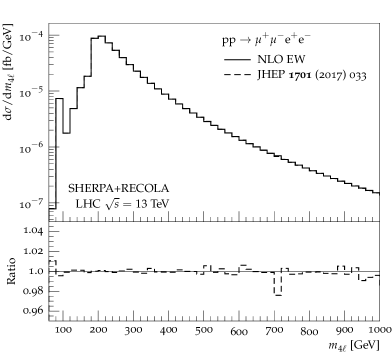
Figure 13: Comparison of the di-muon and four-lepton invariant mass in the process ${\rm pp}\to\mu^{+}\mu^{-}{\rm e}^{+}{\rm e}^{-}$ at NLO EW with the Sherpa ​​+Recola interface compared against the benchmark numbers from Ref. [27]. The upper panel shows the absolute prediction, while the lower panel indicates the ratio between both computations.

In Fig. 13, a comparison of the two independent calculations at the level of NLO EW differential distributions via the di-muon mass $m_{\mu^{+}\mu^{-}}$ and the four-lepton invariant mass $m_{4\ell}$ is presented. Like in the corresponding QCD validation in Section 3.2, the difference in the absolute prediction in the upper panel is almost invisible. The ratio of individual histogram bins in the lower panel shows statistical percent-level fluctuations which illustrate again the excellent agreement. This is a highly non-trivial check, since the benchmark calculation of Ref. [27] has been cross-checked internally by two independent calculations both at the level of the employed matrix elements and at the level of the phase-space integration. Furthermore, the results from Ref. [27] were generated in mass regularisation and slightly different conventions of the dipole subtraction terms.

Combined predictions:

The combined predictions for the total cross section including the QCD corrections from Section 3.2.2 and the EW corrections from this section are stated in Tab. 12.

${\rm pp}\to{\mu^{+}\mu^{-}\text{e}^{+}\text{e}^{-}}$	$\sigma^{\mathrm{LO}}$	$\sigma^{\mathrm{NLO}}_{\mathrm{QCD}+\mathrm{EW}}$	$\delta^{\mathrm{NLO}}_{\mathrm{QCD}+\mathrm{EW}}$	$\sigma^{\mathrm{NLO}}_{\mathrm{QCD}\times\mathrm{EW}}$	$\delta^{\mathrm{NLO}}_{\mathrm{QCD}\times\mathrm{EW}}$
inclusive	$11.498(1)\,$fb	$15.18(1)\,$fb	$32.0(1)\,$%	$14.96(1)\,$fb	$30.1(1)\,$%

Table 12: Integrated cross sections for ${\rm p}{\rm p}\to{\mu^{+}\mu^{-}\text{e}^{+}\text{e}^{-}}$ for a centre-of-mass energy of $\sqrt{s}=13\,\text{TeV}$, calculated with Sherpa ​​+Recola for the set-up of Ref. [27]. The cross sections at LO as well as for the additive and multiplicative combinations of NLO QCD and EW corrections are given. The cross sections are expressed in fb while the relative corrections are given in percent. The integration errors of the last digits are provided in parentheses.

In Fig. 14, different NLO predictions are presented for distributions in the di-muon and four-lepton invariant mass. In the four-lepton invariant-mass distribution, we observe the typical pattern of large negative EW corrections of around $-20\%$ in the high-energy regime at around $1\,\text{TeV}$. The radiative tail below the pair-production threshold at $m_{4\ell}=2M_{\text{Z}}$ with corrections around $+30\%$ is due to the fact that resonant contributions are shifted to lower values by real photon radiation. Since the LO cross section is falling off steeply in this region, the photonic corrections become large. A similar radiative tail is observed also in the di-muon prediction that amounts to positive corrections of up to $+60\%$.

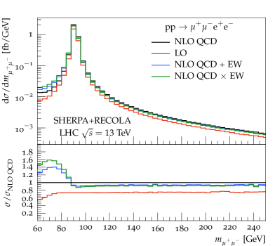
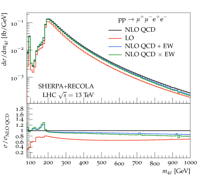
Figure 14: Distributions of the di-muon and four-lepton invariant mass in the process ${\rm pp}\to\mu^{+}\mu^{-}{\rm e}^{+}{\rm e}^{-}$. Results are given for LO, NLO QCD, NLO QCD$+$EW and NLO QCD$\times$EW.

While the QCD corrections are positive over the whole range of both the di-muon and the four-lepton invariant-mass distribution at the order of $+30\%$, the EW corrections exhibit a non-trivial sign change at the Z-boson resonance $m_{\mu^{+}\mu^{-}}=M_{\text{Z}}$ and at the pair-production threshold $m_{4\ell}=2M_{\text{Z}}$, respectively. Further discussion of this issue can be found in Ref. [27].

4.3 Higgs production in association with a top-quark pair

As last example, we consider the on-shell production of a pair of top quarks in association with a Higgs boson. The LO cross section is of order $\mathcal{O}{\left(\alpha_{\text{s}}^{2}\alpha\right)}$. Hence the NLO QCD and EW corrections contribute at order $\mathcal{O}{\left(\alpha_{\text{s}}^{3}\alpha\right)}$ and $\mathcal{O}{\left(\alpha_{\text{s}}^{2}\alpha^{2}\right)}$, respectively. At NLO EW, this computation features QCD–EW interferences. In addition to computing the EW corrections to the QCD-mediated production of the top-quark pairs, one must also consider the QCD corrections to the interference of the QCD and electroweakly produced top-quark pairs. Moreover, the final state consists exclusively of massive particles which is not the case for any of the previously presented processes. This process constitutes thus a non-trivial validation of the implementation. Concerning on-shell top quarks, the process has already been computed at NLO QCD [81, 82, 83, 84, 85] and at NLO EW [86, 87, 88]. It has also been matched to a parton shower [89, 90, 91]. On the other hand, for off-shell top quarks, the NLO QCD [21] and EW [28] corrections have been computed only recently.

Input parameters:

We use the set-up of Ref. [68] which has been described in Section 3.2.3. Concerning the electromagnetic coupling $\alpha$, the $\alpha(M_{\rm Z})$ scheme is employed. Note that contributions originating from initial-state photons are neglected in order to match one of the set-ups of Ref. [68].

NLO EW validation:

As for the QCD validation, we compare five NLO EW cross sections that have been computed by MadGraph5_aMC@NLO and Sherpa ​​+O PEN L OOPS in Ref. [68]. The obtained cross sections are reported in Table 13.

	Sherpa ​​+Recola		MG5_aMC@NLO	Sherpa ​​+O PEN L OOPS
	$\sigma^{\mathrm{NLO}}_{\rm EW}$ [fb]	$\delta_{\rm EW}[\%]$	$\delta_{\rm EW}[\%]$	$\delta_{\rm EW}[\%]$
inclusive	$356.7(2)$	$-1.2(2)$	$-1.4$	$-1.4$
$p_{{\rm T},{\rm t/\bar{t}/H}}>200\,\text{GeV}$	$12.244(3)$	$-8.5(1)$	$-8.5$	$-8.4$
$p_{{\rm T},{\rm t/\bar{t}/H}}>400\,\text{GeV}$	$0.3435(3)$	$-14.1(2)$	$-13.9$	$-14.0$
$p_{{\rm T},{\rm H}}>500\,\text{GeV}$	$1.7798(9)$	$-11.7(1)$	$-11.6$	$-11.7$
$\left|y_{\rm t}\right|>2.5$	$5.035(3)$	$0.3(2)$	$0.5$	$0.5$

Table 13: Integrated cross sections for ${\rm p}{\rm p}\to{\rm t}{\rm\bar{t}}{\rm H}$ at NLO EW for a centre-of-mass energy of $\sqrt{s}=13\,\text{TeV}$ calculated with Sherpa ​​+Recola, MadGraph5_aMC@NLO, and Sherpa ​​+O PEN L OOPS for the set-up of Ref. [68]. The cross sections are expressed in fb, while the relative corrections are given in percent. The integration errors of the last digits are provided in parentheses for the Sherpa ​​+Recola predictions.

Generally good agreement has been found with the results presented in Ref. [68]. Nonetheless, as no statistical errors are stated in the aforementioned reference, an exact comparison has not been possible.

Combined predictions:

Next, combined NLO QCD and EW predictions for the inclusive cross section as well as for a few distributions are presented. No event selection is applied to the final state, meaning that we consider the fully-inclusive production process. The total cross sections at LO and NLO for an additive and multiplicative combination of NLO QCD and EW corrections as defined in Eqs. (13) and (14), respectively, are listed in Table 14.

${\rm pp}\to{\rm t\bar{t}H}$	$\sigma^{\mathrm{LO}}$ [fb]	$\sigma^{\mathrm{NLO}}_{\mathrm{QCD}+\mathrm{EW}}$ [fb]	$\delta^{\mathrm{NLO}}_{\mathrm{QCD}+\mathrm{EW}}$ [%]	$\sigma^{\mathrm{NLO}}_{\mathrm{QCD}\times\mathrm{EW}}$ [fb]	$\delta^{\mathrm{NLO}}_{\mathrm{QCD}\times\mathrm{EW}}$ [%]
inclusive	$361.2(4)$	$459.8(4)$	$27.3(2)$	$458.6(4)$	$27.0(2)$

Table 14: Integrated cross sections for ${\rm p}{\rm p}\to{\rm t}{\rm\bar{t}}{\rm H}$ for a centre-of-mass energy of $\sqrt{s}=13\,\text{TeV}$ calculated with Sherpa ​​+Recola for the set-up of Ref. [68]. The cross sections at LO as well as for the additive and multiplicative combinations of NLO QCD and EW corrections are given. The cross sections are expressed in fb, while the relative corrections are given in percent. The integration errors of the last digits are provided in parentheses.

As the EW corrections are moderate, there are no big differences between the two combinations. This seems to indicate that the missing higher orders of mixed QCD–EW type are small in this case.

In Fig. 15, the transverse momentum as well as the rapidity distribution of the Higgs boson are displayed.

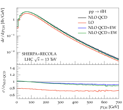
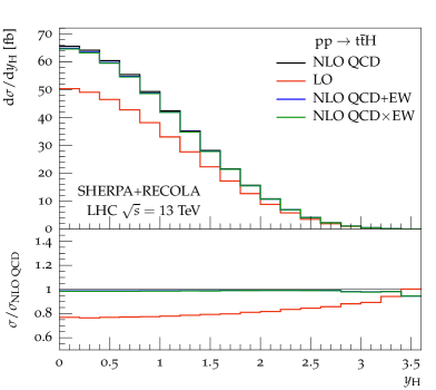
Figure 15: Differential distributions at a centre-of-mass energy $\sqrt{s}=13\,\text{TeV}$ for ${\rm pp}\to{\rm t\bar{t}H}$ at the LHC: transverse-momentum distribution (left) and rapidity distribution of the Higgs boson (right). The lower panels show the ratios $\sigma^{\mathrm{LO}}/\sigma^{\mathrm{NLO}}_{\mathrm{QCD}}$, $\sigma^{\mathrm{NLO}}_{\mathrm{QCD}+\mathrm{EW}}/\sigma^{\mathrm{NLO}}_{\mathrm{QCD}}$ and $\sigma^{\mathrm{NLO}}_{\mathrm{QCD}\times\mathrm{EW}}/\sigma^{\mathrm{NLO}}_{\mathrm{QCD}}$.

The effects of the NLO QCD corrections are dominant over the whole transverse-momentum range and are typically of the order of $25\%$. The EW corrections vary from about $1.2\%$ at zero transverse momentum to $-8.9\%$ at $700\,\text{GeV}$. This behaviour is characteristic for Sudakov logarithms that grow large when all invariants involved in the process become large. In Fig. 16, the distribution of the transverse momentum as well as the rapidity of the top quark are shown.

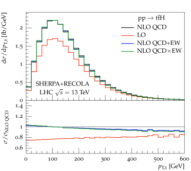
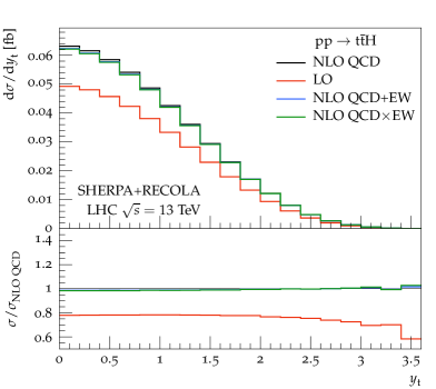
Figure 16: Differential distributions at a centre-of-mass energy $\sqrt{s}=13\,\text{TeV}$ for ${\rm pp}\to{\rm t\bar{t}H}$ at the LHC: transverse-momentum distribution (left) and rapidity distribution of the top quark (right). The lower panels show the ratios $\sigma^{\mathrm{LO}}/\sigma^{\mathrm{NLO}}_{\mathrm{QCD}}$, $\sigma^{\mathrm{NLO}}_{\mathrm{QCD}+\mathrm{EW}}/\sigma^{\mathrm{NLO}}_{\mathrm{QCD}}$ and $\sigma^{\mathrm{NLO}}_{\mathrm{QCD}\times\mathrm{EW}}/\sigma^{\mathrm{NLO}}_{\mathrm{QCD}}$.

Again, the QCD corrections are large over the whole transverse momentum range and amount to at $35\%$ at low transverse momentum to go down to $22\%$ at $p_{{\rm T},\text{t}}=600\,\text{GeV}$. The relative EW corrections also decrease from about $2.6\%$ to reach $-6.7\%$ at $600\,\text{GeV}$.

5 Conclusion

After the very successful Run I, culminating in the discovery of the Higgs boson, the LHC is now operating in the Run II phase. This phase at $\sqrt{s}=13\,\text{TeV}$ might ultimately lead to the discovery of New Physics or confirm, to an even higher degree of accuracy, the theory of the Standard Model of particle physics. In either case, precise (including at least NLO QCD and electroweak corrections) and appropriate (with event selections reproducing the experimental set-ups) predictions for a plethora of Standard Model processes are needed. Such state-of-the-art predictions are, on the one hand, required for precision measurements in the Standard Model. On the other hand, in New Physics searches, they are compulsory to obtain realistic estimates of the Standard Model expectations in order to discriminate possible New Physics contributions. To provide such predictions, public Monte Carlo programs are the ideal tools as they can be used by both the experimental collaborations and the theory community.

In this publication, the combination of the one-loop matrix-element generator Recola with the multipurpose Monte Carlo program Sherpa has been presented. In particular, a short presentation of both codes as well as the main features of the interface have been given. The Sherpa ​​+Recola framework is designed for Standard Model predictions and offers the possibility to compute—in principle—any process at NLO QCD and electroweak accuracy. A large fraction of this article is devoted to the validation of the implementation of Recola in Sherpa. This entails comparisons of squared matrix elements for individual phase-space points, fixed-order cross sections, and differential distributions, as well as the merging/matching of NLO QCD matrix elements with Sherpa’s QCD parton shower. These comparisons are performed against public and private codes as well as results presented in the literature.

Following this validation, predictions have been presented at NLO QCD and electroweak accuracy for three specific processes: both on- and off-shell vector-boson production in association with jets, off-shell ${\rm Z}$-boson pair production, and on-shell production of a top-quark pair in association with a Higgs boson. In addition to their distinguished physical relevance, these processes constitute a good testing ground for this fully automatised implementation. They feature both massive and massless final states, as well as strongly and electroweakly interacting final-state objects. In addition to fixed-order computations, all other functionalities of Sherpa (the QCD parton shower, hadronisation etc.) can be used along with Recola. To demonstrate this, NLO QCD matrix elements for Drell–Yan production in association with multiple QCD jets have been merged and matched to the parton shower. For illustrative purposes, some resulting predictions have been compared to actual LHC data.

The Sherpa ​​+Recola combination is readily publicly available for NLO QCD predictions. The required methods to perform NLO electroweak calculations on the Sherpa side will be made public soon. This ultimately makes it an ideal tool for both experimentalists and theorists to obtain NLO QCD and electroweak accurate predictions for Standard Model processes. It opens the possibility to perform systematic studies on the impact of electroweak corrections for a multitude of LHC production processes.

Appendix A Installation procedures

Recola-1.2 and subsequent versions are compatible with the interface to Sherpa described above. Recola in association with Collier can be downloaded from
http://recola.hepforge.org.
Once downloaded, the following command lines have to be issued:

tar -zxvf recola-collier-1.2.tar.gz
cd recola-collier-1.2
cd build
cmake ..
make

Recola is then installed in association with Collier. Various compilation options can be found in the respective manuals [8, 58]. We note that the Recola library has to be compiled dynamically (this is the default setting) to be used with Sherpa.

The first version of Sherpa compatible with Recola is Sherpa-v2.2.3. It can be downloaded from http://sherpa.hepforge.org.
The installation commands read

tar -zxvf SHERPA-MC-2.2.3.tar.gz
cd SHERPA-MC-2.2.3
autoreconf -i
./configure --enable-recola=/PATH_TO_RECOLA/recola-collier-1.2/recola-1.2 \
[other Sherpa configure options]
make
make install

Extra configuration options can be found in the manual of Sherpa available on the website. After this installation procedure, NLO computations can be readily performed.

Appendix B Specific run-card commands

As mentioned in Section 2.3, some commands allow the user to deviate from the default settings. This appendix is thus devoted to the description of these commands.

On-shell masses for W and Z boson

By default, the input masses for the W and Z bosons are the pole masses. Nonetheless, it is possible to set the on-shell masses instead by including the line

RECOLA_ONSHELLZW=1

in the input run card.

Flavour scheme and quark masses

In order to allow all possible combinations of masses and flavour schemes, a few flags for the run card exist. The first one is

RECOLA_FIXED_FLAVS.

The values 4, 5, and 6 correspond to the corresponding fixed-flavour schemes. Setting the flag to 14, 15, 16 allows for a dynamical scheme up to the number of flavours (4, 5 or 6). Finally, the value $-2$ sets a fixed-flavour scheme according to the masses set in the run card.

It is also possible to set explicitly the masses used in the renormalisation [see Eq. (2)] of the strong coupling using

 RECOLA_AS_REN_MASS_C/B/T,

corresponding to the charm, bottom, and top-quark mass, respectively. On the other hand, the quark masses used for the hard matrix element are read out only from the run card. This means that the user has to take care of the consistency of her/his computation between the matrix element computed and the PDF set used.

UV and IR scales

The UV and IR scales are both set, by default, to a fixed value of $100\,\text{GeV}$. These technical parameters do not impact physical results. However, the choice of the IR scale does change the individual contributions of the virtual corrections and the integrated subtraction terms. In the Sherpa ​​+Recola interface, it is possible to set these scales in the run card, e.g. to directly compare the virtual and real subtraction contributions separately to independent code. These UV and IR scales are set with the keywords

UV_SCALE

and

IR_SCALE,

respectively.

References

- [1] T. Hahn and M. Perez-Victoria, Automatized one loop calculations in four-dimensions and D-dimensions. Comput. Phys. Commun. 118 (1999) 153–165, arXiv:hep-ph/9807565 [hep-ph].
- [2] C. F. Berger et al., Automated implementation of on-shell methods for one-loop amplitudes. Phys.Rev. D78 (2008) 036003, arXiv:arXiv:0803.4180 [hep-ph]. http://inspirebeta.net/record/782271.
- [3] F. Cascioli, P. Maierhöfer, and S. Pozzorini, Scattering Amplitudes with Open Loops. Phys. Rev. Lett. 108 (2012) 111601, arXiv:1111.5206 [hep-ph].
- [4] G. Bevilacqua, M. Czakon, M. V. Garzelli, A. van Hameren, A. Kardos, C. G. Papadopoulos, R. Pittau, and M. Worek, HELAC-NLO. Comput. Phys. Commun. 184 (2013) 986–997, arXiv:1110.1499 [hep-ph].
- [5] V. Hirschi, R. Frederix, S. Frixione, M. V. Garzelli, F. Maltoni, and R. Pittau, Automation of one-loop QCD corrections. JHEP 05 (2011) 044, arXiv:1103.0621 [hep-ph].
- [6] S. Badger, B. Biedermann, P. Uwer, and V. Yundin, Numerical evaluation of virtual corrections to multi-jet production in massless QCD. Comput. Phys. Commun. 184 (2013) 1981–1998, arXiv:1209.0100 [hep-ph].
- [7] G. Cullen et al., GOSAM-2.0: a tool for automated one-loop calculations within the Standard Model and beyond. Eur. Phys. J. C74 (2014) no. 8, 3001, arXiv:1404.7096 [hep-ph].
- [8] S. Actis, A. Denner, L. Hofer, J.-N. Lang, A. Scharf, and S. Uccirati, RECOLA: REcursive Computation of One-Loop Amplitudes. arXiv:1605.01090 [hep-ph].
- [9] A. Cafarella, C. G. Papadopoulos, and M. Worek, Helac-Phegas: A Generator for all parton level processes. Comput. Phys. Commun. 180 (2009) 1941–1955, arXiv:0710.2427 [hep-ph].
- [10] W. Kilian, T. Ohl, and J. Reuter, WHIZARD: Simulating Multi-Particle Processes at LHC and ILC. Eur. Phys. J. C71 (2011) 1742, arXiv:0708.4233 [hep-ph].
- [11] M. Bähr et al., Herwig++ Physics and Manual. Eur. Phys. J. C58 (2008) 639–707, arXiv:0803.0883 [hep-ph].
- [12] T. Gleisberg, S. Höche, F. Krauss, M. Schönherr, S. Schumann, F. Siegert, and J. Winter, Event generation with SHERPA 1.1. JHEP 02 (2009) 007, arXiv:0811.4622 [hep-ph].
- [13] J. Alwall, R. Frederix, S. Frixione, V. Hirschi, F. Maltoni, O. Mattelaer, H. S. Shao, T. Stelzer, P. Torrielli, and M. Zaro, The automated computation of tree-level and next-to-leading order differential cross sections, and their matching to parton shower simulations. JHEP 07 (2014) 079, arXiv:1405.0301 [hep-ph].
- [14] S. Actis, A. Denner, L. Hofer, A. Scharf, and S. Uccirati, Recursive generation of one-loop amplitudes in the Standard Model. JHEP 04 (2013) 037, arXiv:1211.6316 [hep-ph].
- [15] T. Gleisberg, S. Höche, F. Krauss, A. Schälicke, S. Schumann, and J.-C. Winter, SHERPA 1.: A Proof of concept version. JHEP 02 (2004) 056, arXiv:hep-ph/0311263 [hep-ph].
- [16] S. Catani and M. H. Seymour, A general algorithm for calculating jet cross-sections in NLO QCD. Nucl. Phys. B485 (1997) 291–419, arXiv:hep-ph/9605323 [hep-ph]. [Erratum: Nucl. Phys. B510 (1998) 503].
- [17] S. Catani, S. Dittmaier, M. H. Seymour, and Z. Trocsanyi, The dipole formalism for next-to-leading order QCD calculations with massive partons. Nucl. Phys. B627 (2002) 189–265, arXiv:hep-ph/0201036 [hep-ph].
- [18] S. Dittmaier, A general approach to photon radiation off fermions. Nucl. Phys. B565 (2000) 69–122, arXiv:hep-ph/9904440 [hep-ph].
- [19] S. Dittmaier, A. Kabelschacht, and T. Kasprzik, Polarized QED splittings of massive fermions and dipole subtraction for non-collinear-safe observables. Nucl. Phys. B800 (2008) 146–189, arXiv:0802.1405 [hep-ph].
- [20] A. Denner, R. Feger, and A. Scharf, Irreducible background and interference effects for Higgs-boson production in association with a top-quark pair. JHEP 04 (2015) 008, arXiv:1412.5290 [hep-ph].
- [21] A. Denner and R. Feger, NLO QCD corrections to off-shell top-antitop production with leptonic decays in association with a Higgs boson at the LHC. JHEP 11 (2015) 209, arXiv:1506.07448 [hep-ph].
- [22] A. Denner, L. Hofer, A. Scharf, and S. Uccirati, Electroweak corrections to lepton pair production in association with two hard jets at the LHC. JHEP 01 (2015) 094, arXiv:1411.0916 [hep-ph].
- [23] B. Biedermann, M. Billoni, A. Denner, S. Dittmaier, L. Hofer, B. Jäger, and L. Salfelder, Next-to-leading-order electroweak corrections to leptons at the LHC. JHEP 06 (2016) 065, arXiv:1605.03419 [hep-ph].
- [24] B. Biedermann, A. Denner, S. Dittmaier, L. Hofer, and B. Jäger, Electroweak corrections to at the LHC: a Higgs background study. Phys. Rev. Lett. 116 (2016) 161803, arXiv:1601.07787 [hep-ph].
- [25] A. Denner and M. Pellen, NLO electroweak corrections to off-shell top-antitop production with leptonic decays at the LHC. JHEP 08 (2016) 155, arXiv:1607.05571 [hep-ph].
- [26] B. Biedermann, A. Denner, and M. Pellen, Large electroweak corrections to vector-boson scattering at the Large Hadron Collider. arXiv:1611.02951 [hep-ph].
- [27] B. Biedermann, A. Denner, S. Dittmaier, L. Hofer, and B. Jäger, Next-to-leading-order electroweak corrections to the production of four charged leptons at the LHC. JHEP 01 (2017) 033, arXiv:1611.05338 [hep-ph].
- [28] A. Denner, J.-N. Lang, M. Pellen, and S. Uccirati, Higgs production in association with off-shell top-antitop pairs at NLO EW and QCD at the LHC. JHEP 02 (2017) 053, arXiv:1612.07138 [hep-ph].
- [29] S. Kallweit, J. M. Lindert, P. Maierhöfer, S. Pozzorini, and M. Schönherr, NLO electroweak automation and precise predictions for W+multijet production at the LHC. JHEP 04 (2015) 012, arXiv:1412.5157 [hep-ph].
- [30] S. Kallweit, J. M. Lindert, P. Maierhöfer, S. Pozzorini, and M. Schönherr, NLO QCD+EW predictions for V + jets including off-shell vector-boson decays and multijet merging. JHEP 04 (2016) 021, arXiv:1511.08692 [hep-ph].
- [31] S. Kallweit, J. M. Lindert, S. Pozzorini, and M. Schönherr, NLO QCD+EW predictions for diboson signatures at the LHC. arXiv:1705.00598 [hep-ph].
- [32] M. Chiesa, N. Greiner, M. Schönherr, and F. Tramontano, Electroweak corrections to diphoton plus jets. arXiv:1706.09022 [hep-ph].
- [33] F. Krauss, R. Kuhn, and G. Soff, AMEGIC++ 1.0: A Matrix element generator in C++. JHEP 02 (2002) 044, arXiv:hep-ph/0109036 [hep-ph].
- [34] T. Gleisberg and S. Höche, Comix, a new matrix element generator. JHEP 12 (2008) 039, arXiv:0808.3674 [hep-ph].
- [35] T. Binoth et al., A Proposal for a standard interface between Monte Carlo tools and one-loop programs. Comput. Phys. Commun. 181 (2010) 1612–1622, arXiv:1001.1307 [hep-ph].
- [36] T. Gleisberg and F. Krauss, Automating dipole subtraction for QCD NLO calculations. Eur. Phys. J. C53 (2008) 501–523, arXiv:0709.2881 [hep-ph]. http://www.slac.stanford.edu/spires/find/hep/www?eprint=arXiv:0709.2881.
- [37] S. Schumann and F. Krauss, A Parton shower algorithm based on Catani-Seymour dipole factorisation. JHEP 03 (2008) 038, arXiv:0709.1027 [hep-ph].
- [38] S. Höche, S. Schumann, and F. Siegert, Hard photon production and matrix-element parton-shower merging. Phys. Rev. D81 (2010) 034026, arXiv:0912.3501 [hep-ph].
- [39] S. Höche, F. Krauss, S. Schumann, and F. Siegert, QCD matrix elements and truncated showers. JHEP 05 (2009) 053, arXiv:0903.1219 [hep-ph].
- [40] S. Höche, F. Krauss, M. Schönherr, and F. Siegert, QCD matrix elements + parton showers: The NLO case. JHEP 04 (2013) 027, arXiv:1207.5030 [hep-ph].
- [41] S. Höche, F. Krauss, M. Schönherr, and F. Siegert, A critical appraisal of NLO+PS matching methods. JHEP 09 (2012) 049, arXiv:1111.1220 [hep-ph].
- [42] F. Krauss, D. Napoletano, and S. Schumann, Simulating -associated production of and Higgs bosons with the SHERPA event generator. Phys. Rev. D95 (2017) no. 3, 036012, arXiv:1612.04640 [hep-ph].
- [43] E. Bothmann, M. Schönherr, and S. Schumann, Reweighting QCD matrix-element and parton-shower calculations. Eur. Phys. J. C76 (2016) no. 11, 590, arXiv:1606.08753 [hep-ph].
- [44] M. Schönherr in preparation.
- [45] A. Denner, S. Dittmaier, M. Roth, and D. Wackeroth, Predictions for all processes 4 fermions . Nucl. Phys. B560 (1999) 33–65, arXiv:hep-ph/9904472 [hep-ph].
- [46] A. Denner, S. Dittmaier, M. Roth, and L. H. Wieders, Electroweak corrections to charged-current 4 fermion processes: Technical details and further results. Nucl. Phys. B724 (2005) 247–294, arXiv:hep-ph/0505042 [hep-ph]. [Erratum: Nucl. Phys. B854 (2012) 504].
- [47] A. Denner and S. Dittmaier, The complex-mass scheme for perturbative calculations with unstable particles. Nucl. Phys. Proc. Suppl. 160 (2006) 22–26, arXiv:hep-ph/0605312 [hep-ph].
- [48] G. Ossola, C. G. Papadopoulos, and R. Pittau, On the Rational Terms of the one-loop amplitudes. JHEP 05 (2008) 004, arXiv:0802.1876 [hep-ph].
- [49] A. van Hameren, Multi-gluon one-loop amplitudes using tensor integrals. JHEP 07 (2009) 088, arXiv:0905.1005 [hep-ph].
- [50] G. ’t Hooft and M. J. G. Veltman, Scalar one loop integrals. Nucl. Phys. B153 (1979) 365–401.
- [51] W. Beenakker and A. Denner, Infrared divergent scalar box integrals with applications in the electroweak Standard Model. Nucl. Phys. B338 (1990) 349–370.
- [52] S. Dittmaier, Separation of soft and collinear singularities from one-loop N point integrals. Nucl. Phys. B675 (2003) 447–466, arXiv:hep-ph/0308246 [hep-ph].
- [53] A. Denner and S. Dittmaier, Scalar one-loop 4-point integrals. Nucl. Phys. B844 (2011) 199–242, arXiv:1005.2076 [hep-ph].
- [54] G. Passarino and M. J. G. Veltman, One-loop corrections for annihilation into in the Weinberg Model. Nucl. Phys. B160 (1979) 151.
- [55] A. Denner and S. Dittmaier, Reduction of one-loop tensor 5-point integrals. Nucl. Phys. B658 (2003) 175–202, arXiv:hep-ph/0212259 [hep-ph].
- [56] A. Denner and S. Dittmaier, Reduction schemes for one-loop tensor integrals. Nucl. Phys. B734 (2006) 62–115, arXiv:hep-ph/0509141 [hep-ph].
- [57] A. Denner, S. Dittmaier, and L. Hofer, Collier - A fortran-library for one-loop integrals. PoS LL2014 (2014) 071, arXiv:1407.0087 [hep-ph].
- [58] A. Denner, S. Dittmaier, and L. Hofer, Collier: a fortran-based Complex One-Loop LIbrary in Extended Regularizations. Comput. Phys. Commun. 212 (2017) 220–238, arXiv:1604.06792 [hep-ph].
- [59] S. Höche, S. Kuttimalai, S. Schumann, and F. Siegert, Beyond Standard Model calculations with Sherpa. Eur. Phys. J. C75 (2015) 135, arXiv:1412.6478 [hep-ph].
- [60] NNPDF Collaboration, R. D. Ball et al., Parton distributions for the LHC Run II. JHEP 04 (2015) 040, arXiv:1410.8849 [hep-ph].
- [61] NNPDF Collaboration, R. D. Ball, V. Bertone, S. Carrazza, L. Del Debbio, S. Forte, A. Guffanti, N. P. Hartland, and J. Rojo, Parton distributions with QED corrections. Nucl. Phys. B877 (2013) 290–320, arXiv:1308.0598 [hep-ph].
- [62] G. Ossola, C. G. Papadopoulos, and R. Pittau, CutTools: A Program implementing the OPP reduction method to compute one-loop amplitudes. JHEP 03 (2008) 042, arXiv:0711.3596 [hep-ph].
- [63] A. van Hameren, OneLOop: For the evaluation of one-loop scalar functions. Comput. Phys. Commun. 182 (2011) 2427–2438, arXiv:1007.4716 [hep-ph].
- [64] A. Buckley, J. Butterworth, D. Grellscheid, H. Hoeth, L. Lönnblad, J. Monk, H. Schulz, and F. Siegert, Rivet user manual. Comput. Phys. Commun. 184 (2013) 2803–2819, arXiv:1003.0694 [hep-ph].
- [65] M. Cacciari, G. P. Salam, and G. Soyez, The anti- jet clustering algorithm. JHEP 04 (2008) 063, arXiv:0802.1189 [hep-ph].
- [66] M. Cacciari, G. P. Salam, and G. Soyez, FastJet User Manual. Eur. Phys. J. C72 (2012) 1896, arXiv:1111.6097 [hep-ph].
- [67] D. Yu. Bardin, A. Leike, T. Riemann, and M. Sachwitz, Energy-dependent width effects in -annihilation near the Z-boson pole. Phys. Lett. B206 (1988) 539–542.
- [68] J. R. Andersen et al., “Les Houches 2015: Physics at TeV Colliders Standard Model Working Group Report,” in 9th Les Houches Workshop on Physics at TeV Colliders (PhysTeV 2015) Les Houches, France, June 1-19, 2015. 2016. arXiv:1605.04692 [hep-ph]. http://lss.fnal.gov/archive/2016/conf/fermilab-conf-16-175-ppd-t.pdf.
- [69] NNPDF Collaboration, S. Carrazza, Towards the determination of the photon parton distribution function constrained by LHC data. PoS DIS2013 (2013) 279, arXiv:1307.1131 [hep-ph].
- [70] NNPDF Collaboration, S. Carrazza, “Towards an unbiased determination of parton distributions with QED corrections,” in Proceedings, 48th Rencontres de Moriond on QCD and High Energy Interactions, pp. 357–360. 2013. arXiv:1305.4179 [hep-ph]. http://inspirehep.net/record/1234242/files/arXiv:1305.4179.pdf.
- [71] T. Carli, T. Gehrmann, and S. Höche, Hadronic final states in deep-inelastic scattering with Sherpa. Eur. Phys. J. C67 (2010) 73–97, arXiv:0912.3715 [hep-ph].
- [72] CMS Collaboration, V. Khachatryan et al., Measurements of jet multiplicity and differential production cross sections of jets events in proton-proton collisions at 7 TeV. Phys. Rev. D91 (2015) no. 5, 052008, arXiv:1408.3104 [hep-ex].
- [73] ATLAS Collaboration, G. Aad et al., Measurement of the production cross section of jets in association with a Z boson in pp collisions at = 7 TeV with the ATLAS detector. JHEP 07 (2013) 032, arXiv:1304.7098 [hep-ex].
- [74] CMS Collaboration, V. Khachatryan et al., Measurements of the differential production cross sections for a Z boson in association with jets in pp collisions at = 8 TeV. JHEP 04 (2017) 022, arXiv:1611.03844 [hep-ex].
- [75] ATLAS Collaboration, M. Aaboud et al., Measurements of the production cross section of a boson in association with jets in pp collisions at TeV with the ATLAS detector. arXiv:1702.05725 [hep-ex].
- [76] S. Kallweit, J. M. Lindert, S. Pozzorini, M. Schönherr, and P. Maierhöfer, “NLO QCD+EW automation and precise predictions for V+multijet production,” in Proceedings, 50th Rencontres de Moriond, QCD and high energy interactions: La Thuile, Italy, March 21-28, 2015, pp. 121–124. 2015. arXiv:1505.05704 [hep-ph]. https://inspirehep.net/record/1372103/files/arXiv:1505.05704.pdf.
- [77] J. Ohnemus and J. F. Owens, An order calculation of hadronic production. Phys. Rev. D43 (1991) 3626–3639.
- [78] B. Mele, P. Nason, and G. Ridolfi, QCD radiative corrections to Z boson pair production in hadronic collisions. Nucl. Phys. B357 (1991) 409–438.
- [79] L. J. Dixon, Z. Kunszt, and A. Signer, Vector boson pair production in hadronic collisions at order : Lepton correlations and anomalous couplings. Phys. Rev. D60 (1999) 114037, arXiv:hep-ph/9907305 [hep-ph].
- [80] J. M. Campbell and R. K. Ellis, An update on vector boson pair production at hadron colliders. Phys. Rev. D60 (1999) 113006, arXiv:hep-ph/9905386 [hep-ph].
- [81] W. Beenakker, S. Dittmaier, M. Krämer, B. Plümper, M. Spira, and P. M. Zerwas, Higgs radiation off top quarks at the Tevatron and the LHC. Phys. Rev. Lett. 87 (2001) 201805, arXiv:hep-ph/0107081 [hep-ph].
- [82] W. Beenakker, S. Dittmaier, M. Krämer, B. Plümper, M. Spira, and P. M. Zerwas, NLO QCD corrections to production in hadron collisions. Nucl. Phys. B653 (2003) 151–203, arXiv:hep-ph/0211352 [hep-ph].
- [83] L. Reina and S. Dawson, Next-to-leading order results for production at the Tevatron. Phys. Rev. Lett. 87 (2001) 201804, arXiv:hep-ph/0107101 [hep-ph].
- [84] S. Dawson, L. H. Orr, L. Reina, and D. Wackeroth, Associated top quark Higgs boson production at the LHC. Phys. Rev. D67 (2003) 071503, arXiv:hep-ph/0211438 [hep-ph].
- [85] S. Dawson, C. Jackson, L. H. Orr, L. Reina, and D. Wackeroth, Associated Higgs production with top quarks at the large hadron collider: NLO QCD corrections. Phys. Rev. D68 (2003) 034022, arXiv:hep-ph/0305087 [hep-ph].
- [86] S. Frixione, V. Hirschi, D. Pagani, H. S. Shao, and M. Zaro, Weak corrections to Higgs hadroproduction in association with a top-quark pair. JHEP 09 (2014) 065, arXiv:1407.0823 [hep-ph].
- [87] Y. Zhang, W.-G. Ma, R.-Y. Zhang, C. Chen, and L. Guo, QCD NLO and EW NLO corrections to production with top quark decays at hadron collider. Phys. Lett. B738 (2014) 1–5, arXiv:1407.1110 [hep-ph].
- [88] S. Frixione, V. Hirschi, D. Pagani, H. S. Shao, and M. Zaro, Electroweak and QCD corrections to top-pair hadroproduction in association with heavy bosons. JHEP 06 (2015) 184, arXiv:1504.03446 [hep-ph].
- [89] R. Frederix, S. Frixione, V. Hirschi, F. Maltoni, R. Pittau, and P. Torrielli, Scalar and pseudoscalar Higgs production in association with a top-antitop pair. Phys. Lett. B701 (2011) 427–433, arXiv:1104.5613 [hep-ph].
- [90] M. V. Garzelli, A. Kardos, C. G. Papadopoulos, and Z. Trocsanyi, Standard Model Higgs boson production in association with a top anti-top pair at NLO with parton showering. Europhys. Lett. 96 (2011) 11001, arXiv:1108.0387 [hep-ph].
- [91] H. B. Hartanto, B. Jäger, L. Reina, and D. Wackeroth, Higgs boson production in association with top quarks in the POWHEG BOX. Phys. Rev. D91 (2015) 094003, arXiv:1501.04498 [hep-ph].