The Gauge-Higgs Legacy of the LHC Run I
Abstract
The effective Lagrangian expansion provides a framework to study effects of new physics at the electroweak scale. To make full use of LHC data in constraining higher-dimensional operators we need to include both the Higgs and the electroweak gauge sector in our study. We first present an analysis of the relevant di-boson production LHC results to update constraints on triple gauge boson couplings. Our bounds are several times stronger than those obtained from LEP data. Next, we show how in combination with Higgs measurements the triple gauge vertices lead to a significant improvement in the entire set of operators, including operators describing Higgs couplings.
I Introduction
The direct exploration of the electroweak symmetry breaking sector started with the discovery of a light narrow Higgs boson higgs in 2012 discovery — a triumph of particle physics. Already the LHC Run I allowed ATLAS and CMS to perform a large number of tests of the nature of the observed resonance, but no significant deviations from the Standard Model properties were observed for example in the Higgs production and decay rates legacy ; other_final_fits ; other_final_fits2 ; Ellis:2014jta . On the other hand, it is important to remind ourselves that the current constraints are still at a precision level for which no significant deviations would be expected in weakly interacting models of new physics bsm_review .
If we accept the Standard Model assumption that the Higgs particle is closely related to the massive gauge bosons, the Higgs results from Run I should be combined with corresponding precision measurements in the electroweak sector. During Run I the LHC collaborations have also collected meaningful event samples probing electroweak gauge boson pair production. They contain information on the structure of the triple gauge boson vertices (TGV)s and allow for complementary tests of the electroweak symmetry breaking mechanism.
The eventual observation of departures of Higgs or gauge boson couplings from their SM predictions can give hints of physics beyond the Standard Model, affecting the electroweak sector and characterized by a new energy scale . One way of parametrizing low–energy effects of SM extensions is by means of an effective Lagrangian effective , which only depends on the low–energy particle content and symmetries. This bottom–up approach has the advantage of minimizing the amount of theoretical hypothesis when studying deviations from the SM predictions. Here, we assume that the observed Higgs–like state belongs to a light electroweak doublet and that the symmetry is linearly realized in the effective theory effective-linear ; kilian ; higgsmultiplets ; kaoru ; Grzadkowski:2010es . Without lepton number violation, the lowest order operators which can be built are of dimension six. The coefficients of these dimension–six operators parametrize our ignorance of the new physics effects and have to be determined using all available data.
One result of this effective theory approach is that modified Higgs couplings to weak bosons are related to triple gauge boson vertices in a model independent fashion. This allows us to use Higgs data not only to constrain TGVs barca2 , but also to use TGV data to test the strengths and structures of Higgs couplings. Usually, such combined analyses rely on LEP results for the TGVs barca ; Brivio:2013pma ; Falkowski:2015jaa , the only exception being Ref. Ellis:2014jta . The reason is that LEP provided the strongest constraints on TGVs until now. However, during the LHC Run I both ATLAS and CMS have collected a substantial amount of data on di-boson searches. It contains information on TGVs, whose relevance has not been addressed quantitatively. We fill this void with the first global analysis of the complete di-boson and Higgs data from the LHC Run I.
The outline of the paper is as follows: after briefly reviewing the relevant set of operators in Sec. II, we present the results of our global analysis of the LHC Run I data on di-boson searches in Sec. III. We find that the combined LHC Run I results are substantially stronger than the LEP constraints. Section IV contains the combined analysis of di-boson and Higgs data, giving the up-to-date limits on the ten relevant Wilson coefficients. We summarize in Sec. V. The details of our di-boson simulations can be found in the Appendix A.
II Theoretical framework
In the linear effective Lagrangian expansion we construct a -symmetric Lagrangian based on the SM field content, including the Higgs-Goldstone doublet . We order the Lagrangian according to the inverse powers of the new physics scale effective-linear ; kilian ; higgsmultiplets ; kaoru ; Grzadkowski:2010es ,
| (1) |
where is the natural choice for a matching scale with a given complete theory. Neglecting the dimension–five lepton number violating operator the next order of the expansion is based on dimension–six operators.
The minimum independent set consists of 59 baryon number conserving operators, barring flavor structure and Hermitian conjugation Grzadkowski:2010es . We follow the definition of the relevant operator basis for LHC Higgs and TGV physics described in detail in Ref. barca . We start by restricting the initial set to and –even operators. We then use the equations of motion to rotate to a basis where there are no blind directions linked to electroweak precision data. In practice, we can neglect all operators contributing to electroweak precision observables at tree level; they are strongly constrained by the several low energy measurements, rendering them irrelevant for current Higgs and TGV studies at the LHC. We then neglect all operators that cannot be studied at the LHC yet, because they only contribute to interactions we are not sensitive to. This includes the vertex or the Higgs interactions with light-generation fermions. Finally, we are left with ten dimension–six operators barca :
| (2) | ||||||||
In our conventions the Higgs doublet covariant derivative is . The hatted field strengths are and , where are the Pauli matrices, and and stand for the and gauge couplings. The adjoint Higgs field is . The effective Lagrangian which we use to interpret Higgs and TGV measurements at the LHC is
| (3) |
All operators except for contribute to Higgs interactions. Their contributions to the several Higgs vertices, including non–SM Lorentz structures, are described in Ref. legacy .
Some of the operators in Eq. (2) contribute to the self-interactions of the electroweak gauge bosons. They can be linked to specific deviations in the Lorentz structures entering the and interactions, usually written as , , and Hagiwara:1986vm . After is fixed to unity because of electromagnetic gauge invariance, writing the deviations with respect to the SM values for example as , the shifts are defined as
| (4) |
where and . The two notational conventions are linked as
| (5) | ||||||||
The -gauge-invariant formulation in terms of dimension–six operators induces correlations of the formerly multi-dimensional space of modified gauge couplings,
| (6) |
This defines what is usually referred to as the LEP scenario in the analysis of anomalous TGV interactions. The three relevant Wilson coefficients relevant for our analysis of di-boson production are , and .
III Triple gauge boson interactions
In our analysis we describe the measured di-boson production rates from the LHC Run I in terms of the Lagrangian given in Eq. (4). We include the eight di-boson measurements with the highest sensitivity for charged triple gauge boson vertices. Adding the public LHC results, only available for 7 TeV so far cms7wa ; atlas7wa , does not improve our results.
For each analysis we first determine which of the kinematic distributions given in the publications is most sensitive to anomalous TGVs. This defines our list of channels and kinematic variables, as well as the available number of bins of the distribution.
| Channel | Distribution | # bins | Data set |
|---|---|---|---|
| Leading lepton | 4 | ATLAS 8 TeV, 20.3 fb-1 atlas8ww | |
| 8 | CMS 8 TeV, 19.4 fb-1 cms8ww | ||
| 6 | ATLAS 8 TeV, 20.3 fb-1 atlas8wz | ||
| candidate | 10 | CMS 8 TeV, 19.6 fb-1 cms78wz | |
| candidate | 12 | ATLAS 7 TeV, 4.6 fb-1 atlas7semilep | |
| candidate | 10 | CMS 7 TeV, 5.0 fb-1 cms7semilep | |
| candidate | 7 | ATLAS 7 TeV, 4.6 fb-1 atlas7wz | |
| candidate | 8 | CMS 7 TeV, 4.9 fb-1 cms78wz |
In the final states only are considered, channels with include a jet veto, and the two semileptonic channels include a veto on a third hard jet.
III.0.1 Analysis framework
Directly from the relevant experimental figure we read off the background expectation (defined as all SM processes except for the di-boson production channels), the expected contribution from production in the Standard Model and the measured event number bin by bin. The background rates we use directly from the experimental analysis, without any need to modify them. Next, we simulate SM production in the fiducial region using MadGraph5 madgraph for the event generation, Pythia Sjostrand:2006za for parton shower and hadronization, and Delphes delphes for the detector simulation. We compare these results to the experimental predictions, defining a bin-by-bin correction factor. It accounts for phase–space dependent corrections either from detector effects or from higher order corrections nloww . These correction factors we apply to our simulated distributions in the presence of the anomalous TGVs, based on an in-house MadGraph5 implementation of the operators constructed with FeynRules Christensen:2008py . In the Appendix we give more details on this procedure for one of the leading experimental channels, i.e. the leptonic ATLAS production at 8 TeV atlas8ww .
We check this default procedure using an alternative setup where instead of matching our SM distributions bin-by-bin, we only match our inclusive rate prediction in the Standard Model in the signal region. Both methods give consistent results for the combined analysis.
The parameter determination relies on SFitter, for technical details we refer to Refs. sfitter_orig ; sfitter_delta ; legacy . We first construct Markov chains in the three-dimensional model space of , and . Then we build the likelihood function for the given data set and determine the part of parameter space allowed at a given CL. In the construction of the likelihood we always include Poisson-shaped statistical uncertainties for event numbers, a Gaussian-shaped experimental systematic uncertainty and a flat theory uncertainty for the signal. As experimental systematics we include the biggest sources of uncertainties for a given experiment, this includes the luminosity estimate, detector and lepton reconstruction/isolation uncertainties, and some additional uncertainty for the background normalization and/or shape, all discussed in the Appendix. For the theoretical uncertainty we allow for a variation of 5% for , 4% for and 4% for -semileptonic channels. We fully correlate theoretical uncertainties for sets with the same di-boson final state.
Wherever the experimental collaborations present their results in terms of anomalous TGVs we validate our procedure through a detailed comparison with their results as exemplified in the Appendix A.
III.0.2 Results from LHC Run I
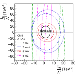
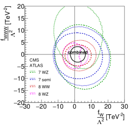
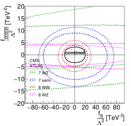
In Fig. 1 we show the results of our pure TGV analysis in terms of the Wilson coefficients defined in Eq. (3). In addition to each individual ATLAS and CMS channel we give the combined constraints from all eight channels. For the combination, we find a global minimum at a Gauss-equivalent for a total of 65 data points, while for the Standard Model. The regions allowed by the different searches are mutually compatible and show no significant preference for a deviation from the Standard Model. Moreover, the structure of the parameter space is simple enough that none of the two-dimensional planes significantly change if instead of a profile likelihood we show a slice where the third Wilson coefficient is zero.
The Wilson coefficient is the least constrained because it hardly affects the vertex since its contribution is suppressed by a factor . Instead, the constraints on come from the fully leptonic searches and to some degree from the -semileptonic analyses, both probing the interaction. The ATLAS channel at 8 TeV sets the strongest bounds on .
Comparing and , we notice that the combination of the and vertices with the large transverse momentum available at the LHC leads to similar sensitivities on both; equivalently, we find comparable sensitivities on and . The new physics reach in and is clearly stronger than in . The strongest bounds on stem from the combination of the two 8 TeV leptonic searches together with the ATLAS 8 TeV analysis. In the case of , the 8 TeV analyses present a higher sensitivity, but again the 8 TeV searches are close in their precision. The constraint on benefits most from a combination of the different experimental channels.
Generally, even though the -semileptonic results presented here are less sensitive to the dimension–six operators, they are not far from the most powerful leptonic and analyses. This is remarkable, given the fact that these semileptonic measurements are still based on the 7 TeV smaller data sets. An update of the semileptonic channels should significantly contribute to a global TGV analysis.
The one-dimensional 95% CL constraints on the combination of Wilson coefficients are
| (7) |
The same results can also be expressed as
| (8) |
where the bounds stand for the limits obtained assuming a negative (positive) Wilson coefficient. Moreover, we can present our results in terms of three independent TGV couplings Hagiwara:1986vm , as described in Sec. II, the 95% CL constraints then read
| (9) |
One aspect that we have tested is how robust our results are when we change our approximate treatment of fully correlated theoretical uncertainties. It turns out that removing these correlations slightly shifts the range towards negative values and weaken the bound on ; both effects are at the level of less than 0.5 standard deviations.
To allow for an easy presentation of the approximate fit results we perform a Gaussian fit to the multi-dimensional probability distribution function of the three Wilson coefficients relevant for TGVs. For the mean, one standard deviation and the error correlation matrix we find
| (10) |
The corresponding Gaussian fit results to the multi-dimensional probability distribution function for the TGV couplings in Eq. 5 are shown in Table 1.
III.0.3 Comparison and combination with LEP
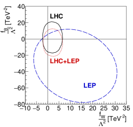
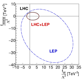
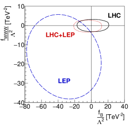
When we express our results in terms of the TGVs defined in Eq. (5) we can easily compare them and eventually combine them with the global LEP analysis results LEP2002 . We show the separated LHC Run I and LEP limits in Table 1. As we can see, the combined LHC Run I di-boson channels determine the anomalous TGV parameters a factor 3-6 more precisely than LEP. Moreover, the more diverse set of LHC observables implies that the different coupling measurements are less correlated.
| LHC Run I | LEP | |||||||
|---|---|---|---|---|---|---|---|---|
| 68 % CL | Correlations | 68 % CL | Correlations | |||||
The same comparison between the combined LHC Run I results and the LEP bounds is illustrated in Fig. 2, now in terms of dimension-six Wilson coefficients. In these two-dimensional profile likelihoods we also show the statistical combination of the two data sets. While the LHC precision shown in Eq. (7) clearly dominates the combination of LHC and LEP results, we still quote the combined limits on the three relevant Wilson coefficients,
| (11) |
Adding the LEP results does not lead to a significant improvement. The range for slightly shifts towards more negative values as a consequence of the preferred LEP central values.
IV Gauge–Higgs combination


In the final step of our effective field theory analysis, we have to combine the LHC Run I results on TGVs and Higgs couplings. The main reason is that and contribute to anomalous Higgs interactions and the triple gauge boson interactions at the same time Hagiwara:1993qt ; barca ; barca2 . Consequently, a study of the underlying Wilson coefficients should include both sets of experimental analyses. Furthermore, the combination of the two can be used to test the nature of the electroweak symmetry breaking mechanism Brivio:2013pma .
For the sake of comparison we start with a brief summary of the global analysis of the LHC Run I Higgs data presented in Ref. legacy , where constraints on the dimension-six Wilson coefficients in Eq. (3) are derived from Higgs measurements alone. That data consists of 159 observables for event rates, plus 14 additional measurements related to kinematics. This kinematic information is crucial to disentangle the strongly correlated effects of non–SM Lorentz structures generated by , , , and . This way, the kinematic distributions significantly improve the global Higgs fit.
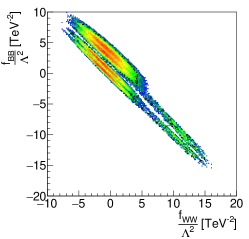
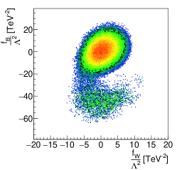
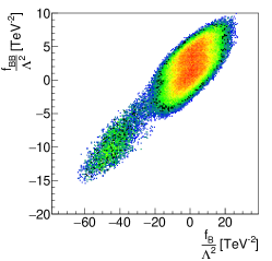
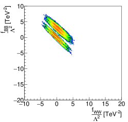
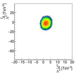
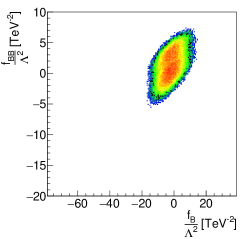
As an illustration, we show three of the relevant two-dimensional profile likelihoods from the pure Higgs analysis including kinematic distributions in the first row of Fig. 3. In the upper-left panel we see a strong correlation between and , even after including the kinematic distributions. This is due to both operators contributing to the decay rate . Without kinematic information the wide pattern in the upper left part simply extends to the lower right part legacy . The improvement in the region of large positive (negative) () appears because both operators contribute to the and vertices, to which the kinematic distributions are sensitive. In the upper-center panel we show the correlations between and . While the kinematic distributions significantly improve the situation, a secondary region still remains for negative . Finally, in the upper-right panel we show the vs plane. Again, the kinematic information largely removes the strong correlations for negative and values.
In the lower panels of Fig. 3 we depict the same two-dimensional profile likelihoods once we include the di-boson TGV measurements from LHC Run I; although LEP limits hardly have any numerical effect, they are included as well. We construct the global likelihood accounting for the correlations in systematic uncertainties between the Higgs observables and the TGV observables. This can be easily achieved in the SFitter framework described in Sec. III and Ref. legacy . The systematic experimental uncertainties are assumed to be correlated for observables in ATLAS and in CMS, but uncorrelated between the two experiments.
For all three panels the effect of the TGV measurements is remarkable. The combination of Higgs and TGV results clearly deliver stronger limits than either of the two analyses independently. The secondary solution in has vanished altogether, the precision on has improved, negative values of are excluded through correlations with , and in the correlation of and we can clearly see two different regions corresponding to sign changes in the coupling.
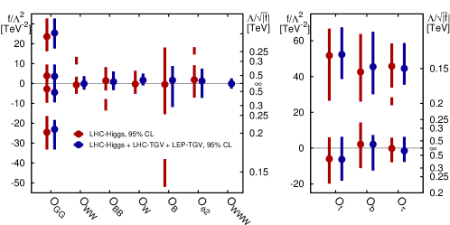
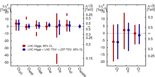
In Table 2 and Fig. 4 we show the limits on individual Wilson coefficients for each of the dimension–six operators included in the analysis, Eq. (3). In the upper panels of Fig. 4 and in the table we clearly see secondary solutions due to sign flips in the individual Yukawa and couplings. In the lower panels of Fig. 4 we show only the solutions for parameter space with SM signs of the Yukawa couplings, and focusing on the containing the SM point, extending our set of simplifications discussed in Sec. II. In both cases we see that the limits including di-boson channels are significantly improved. This improvement is driven by the highest sensitivity we have derived on and , which feeds through to the remaining operators because of the existing correlations. Including the di-boson data removes all secondary solutions from non-trivial parameter correlations or strong non-Gaussian effects. The additional Wilson coefficient is among the best-measured dimension–six modification in the gauge–Higgs sector studied here.
| LHC–Higgs | LHC–Higgs + LHC–TGV + LEP–TGV | |||
| Best fit | 95% CL interval | Best fit | 95% CL interval | |
| 3.9 | 3.6 | |||
| 23.6 | 25.4 | |||
| 1.4 | 0.9 | |||
| 1.9 | 1.3 | |||
| 1.7 | ||||
| 1.7 | ||||
| —– | -0.06 | |||
| 2.2 | 2.2 | |||
| 42.6 | 45.6 | |||
| 45.8 | 44.5 | |||
| 51.8 | 52.3 | |||
| , | , | |||
One caveat applies to these results the same way it applies to the Higgs analysis alone legacy ; d6_vs_eft . If we consider the Lagrangian of Eq. (3) to be the leading term in a systematic effective field theory, we have to ensure that only data probing typical momentum ranges below enters our analysis. Otherwise, neglected dimension–eight and higher operators might lead to large effects. This condition may not always be fulfilled in all the bins of the kinematic distributions studied here depending on the assumed size of the Wilson coefficients, as illustrated in the Appendix. Therefore, we refrain from interpreting our results in terms of an effective field theory and instead consider Fig. 4 as limits on a truncated dimension-six Lagrangian.
V Summary
We have presented a final analysis of the LHC Run I measurements related to weak boson self-interactions and Higgs decays in the framework of an effective Lagrangian to dimension–six. The parameter space for this analysis spans over 10 relevant Wilson coefficients given in Eq. (3). All of them can be strongly constrained by the combination of Higgs and di-boson data.
For triple gauge-boson data we give the first combination of all the di-boson production channels at LHC Run I, relevant to constrain the three dimension–six operators contributing. The current bounds derived in Sec. III are a factor 3-6 more precise than the corresponding LEP bounds. Since LHC Run I is sensitive to the TGVs in a diverse set of channels, the allowed parameter ranges for the couplings are only weakly correlated; see Eq. (10). In the future, we expect sizeable progress in particular for channels with semi-leptonic decays of weak-boson pairs.
In Sec. IV we combine the Run I di-boson data with the Run I Higgs measurements legacy . This leads to a significant improvement compared to both individual analyses. While in the Higgs analysis alone we are left with strong correlations between the different Wilson coefficients — leading to large non-Gaussian structures in the correlated likelihood — secondary solutions in the combined analysis are exclusively due to the signs of the Yukawa couplings. Furthermore, the use of the Higgs data leads to an improvement on the determination of TGVs, specially . Our results shown in Fig. 4 clearly indicate that di-boson data should be part of any effective Lagrangian analysis of the Higgs sector at the LHC.
Acknowledgments
A.B. is supported by the Heidelberg Graduate School for Fundamental Physics and the Graduiertenkolleg Particle Physics beyond the Standard Model. O.J.P.E. is supported in part by Conselho Nacional de Desenvolvimento Científico e Tecnológico (CNPq) and by Fundação de Amparo à Pesquisa do Estado de São Paulo (FAPESP). M.C.G-G acknowledges support from USA-NSF grant PHY-13-16617, EU grant FP7 ITN INVISIBLES (Marie Curie Actions PITN-GA-2011-289442), FP10 ITN ELUSIVES (H2020-MSCA-ITN-2015-674896), INVISIBLES-PLUS (H2020-MSCA-RISE-2015-690575), Spanish grants 2014-SGR-104 and by FPA2013-46570 and consolider-ingenio 2010 program CSD-2008-0037.
Appendix A ATLAS WW analysis
In this appendix we describe in detail how we include the experimental results in our SFitter analysis. As an example we use one of the most sensitive channels, namely the leptonic ATLAS analysis based on of 8 TeV data atlas8ww . One advantage of this analysis is that ATLAS presents their results in terms of TGVs, which allows us to compare their results with the ones of our SFitter implementation. The other seven channels are treated exactly in the same way.
We start by generating events with SM couplings using MadGraph5 madgraph , Pythia Sjostrand:2006za for parton shower and hadronization, and Delphes delphes for fast detector simulation. We model here the ATLAS selection, which is very similar to the analogous CMS analysis cms8ww . The selection procedure requires exactly one electron and one muon of opposite charges in the central detector and outside the transition regions,
| (12) | ||||||||
In addition, the summed transverse energy within a cone of around each lepton is required to be smaller than 14% of , and the scalar sum of the of the tracks within the same cone has to stay below 10% of for the electron and 12% for the muon. A third lepton is vetoed for GeV, as are jets with GeV and . The latter removes the top pair background. A set of requirements on missing energy related variables starts with a requirement on , constructed as the length of the negative 2-vectorial sum of all identified leptons and tracks not associated with leptons atlas8ww . To select events with neutrinos ATLAS requires
| (13) |
A second missing energy variable has to fulfill
| (14) |
where is the azimuthal angle between the missing transverse momentum vector and the nearest lepton.
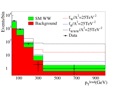
We use the SM events rates in the signal region to tune our event generation, both in terms of the total rate and in the most relevant kinematic distribution. For the latter, we identify the kinematic distribution which is most sensitive to anomalous TGVs and which we will later include in our SFitter analysis. Of the variables and ranges shown in the ATLAS note, the leading has the largest potential because it tracks the momentum flow through the anomalous vertex best Eboli:2010qd ; anke_johann . This means that our event generation has to reproduce Fig. 11 in Ref. atlas8ww . To ensure this, we introduce a bin-by-bin correction factor to account for differences in the selection procedure because of detector effects as well as higher order corrections to the cross section prediction nloww .
Assuming that the same bin-by-bin correction from the SM events applies to the relatively small new physics effects, we generate the leading distribution in the presence of dimension–six operators. For this we rely on MadGraph5 and an in-house implementation of the operators through FeynRules Christensen:2008py . As is well known higher dimensional operators give rise to fast growth of the scattering amplitude with energy, eventually violating partial-wave unitarity Corbett:2014ora . Here we did not introduce ad-hoc form factors to dampen the scattering amplitude at high energies because we verified that there is no partial-wave unitarity violation in the different channels for the values of the Wilson coefficients in the 95% CL allowed regions, except for very large and already ruled out values of .
The predicted number of events for a given Wilson coefficient is the sum of SM and new physics events, together with the SM backgrounds which we directly extract from the ATLAS documentation. These backgrounds are dominated by top production, followed by +jets and Drell-Yan events. All of them are estimated using data-driven techniques. Only the small di-boson backgrounds are based on Monte Carlo estimates atlas8ww .
In Fig. 5 we show the final estimates for the SM background and the SM prediction for production. They are in agreement with the number of observed events. The dashed lines illustrate the effects from individual dimension-six operators, suggesting that we should be able to derive powerful constraints from the ATLAS measurements. The fact that the last bin extends to very large transverse momenta also suggests that we have to be careful interpreting our dimension-six analysis in terms of an effective field theory expansion legacy ; d6_vs_eft .

In the final step of the Sfitter analysis we construct a likelihood function including a Poisson-shaped statistical uncertainty for the observed number of events for each bin, a Poisson-shaped statistical uncertainty for the background events, a flat theoretical uncertainty correlating between all bins in the distribution, and a selection of the most relevant systematic uncertainties with a Gaussian shape. These uncertainties can be seen in the following, together with the selection of experimental systematic uncertainties considered for the rest of the analyses.
| Channel | Exp | Luminosity | Detector eff | Lepton eff | Background rate |
|---|---|---|---|---|---|
| atlas8ww | ATLAS | 2.0% | 1.4% | 1.4% | 2.0% |
| cms8ww | CMS | 2.6% | 1.0% | 3.8% | 2.0% |
| atlas8wz | ATLAS | 2.8% | 0.5% | 1.7% | 1.6% |
| cms78wz | CMS | 4.4% | 3.1% | 2.0% | 2.5% |
| atlas7semilep | ATLAS | 1.8% | 10% | 1.1% | 14% |
| cms7semilep | CMS | 2.2% | 1.0% | 2.0% | – |
| atlas7wz | ATLAS | 1.8% | 0.5% | 1.9% | – |
| cms78wz | CMS | 2.2% | 3.8% | 2.4% | 5.5% |
For the cases where we quote no numbers we assume that those systematic uncertainties are well below the statistical and theoretical uncertainties. For the pure TGV analysis we construct Markov chains to probe the three-dimensional parameter space spanned by , and . Based on these chains we determine the part of the parameter space allowed at a given CL.
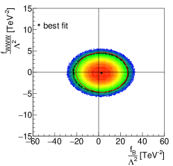
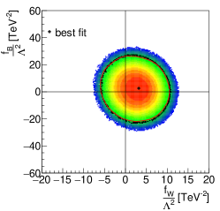
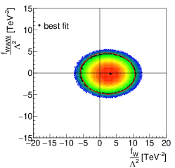
In Fig. 6 we show the three two-dimensional profile likelihoods for the three relevant Wilson coefficients. We find the best-fit point for a mildly positive value of , driven by a small deficit of events in the tail of the leading distribution shown in Fig. 5. The SM gives , defined after profiling over the theoretical uncertainties, and is perfectly compatible with the best fit point at . We have checked that none of these results change if we replace the profile likelihood by a slice of parameter space setting the third Wilson coefficient to zero.
The black dots in Fig. 6 indicate our 95% CL contour and allow us to compare with the red line, that illustrates the 95% CL region from the anomalous TGV analysis by ATLAS atlas8ww . Both are in excellent agreement with each other, indicating that our approximations concerning detector effects or higher order corrections are more than sufficient given the current reached precision of the analysis.
We follow a similar procedure for all eight di-boson channels. Among those the 8 TeV CMS analysis cms8ww and the semi-leptonic 7 TeV ATLAS analysis atlas7semilep quote limits on dimension–six operators from the measurement of anomalous TGVs in the framework of Eq. (6). In both cases we find a similar level of agreement.
References
- (1) P. W. Higgs, Phys. Lett. 12, 132 (1964); P. W. Higgs, Phys. Rev. Lett. 13, 508 (1964); F. Englert and R. Brout, Phys. Rev. Lett. 13, 321 (1964).
- (2) G. Aad et al. [ATLAS Collaboration], Phys. Lett. B 716, 1 (2012), S. Chatrchyan et al. [CMS Collaboration], Phys. Lett. B 716, 30 (2012).
- (3) T. Corbett, O. J. P. Eboli, D. Goncalves, J. Gonzalez-Fraile, T. Plehn and M. Rauch, JHEP 1508, 156 (2015) [arXiv:1505.05516 [hep-ph]], and [arXiv:1511.08188 [hep-ph]].
- (4) G. Aad et al. [ATLAS Collaboration], Phys. Lett. B 726, 88 (2013) Erratum: [Phys. Lett. B 734, 406 (2014)], S. Chatrchyan et al. [CMS Collaboration], JHEP 1306, 081 (2013).
- (5) G. Belanger, B. Dumont, U. Ellwanger, J. F. Gunion and S. Kraml, Phys. Rev. D 88, 075008 (2013); P. P. Giardino, K. Kannike, I. Masina, M. Raidal and A. Strumia, JHEP 1405, 046 (2014); P. Bechtle, S. Heinemeyer, O. Stal, T. Stefaniak and G. Weiglein, JHEP 1411, 039 (2014); K. Cheung, J. S. Lee and P. Y. Tseng, Phys. Rev. D 90, 095009 (2014); J. B. Flament, arXiv:1504.07919 [hep-ph]. B. Dumont, S. Fichet and G. von Gersdorff, JHEP 1307, 065 (2013); S. Fichet and G. Moreau, Nucl. Phys. B 905, 391 (2016); G. Buchalla, O. Cata, A. Celis and C. Krause, arXiv:1511.00988 [hep-ph]; C. Englert, R. Kogler, H. Schulz and M. Spannowsky, arXiv:1511.05170 [hep-ph]; L. Reina, J. de Blas, M. Ciuchini, E. Franco, D. Ghosh, S. Mishima, M. Pierini and L. Silvestrini, PoS EPS-HEP2015, 187 (2015); S. Banerjee, S. Mukhopadhyay and B. Mukhopadhyaya, Phys. Rev. D 89, no. 5, 053010 (2014); L. Bian, J. Shu and Y. Zhang, JHEP 1509, 206 (2015).
- (6) J. Ellis, V. Sanz and T. You, JHEP 1407, 036 (2014) and JHEP 1503, 157 (2015).
- (7) See e.g. C. Englert, A. Freitas, M. M. Mühlleitner, T. Plehn, M. Rauch, M. Spira and K. Walz, J. Phys. G 41, 113001 (2014).
- (8) S. Weinberg, Physica 96A, 327 (1979); see also H. Georgi, Weak Interactions and Modern Particle Theory (Benjamim/Cummings, Menlo Park, 1984) and J. F. Donoghue, E. Golowich and B. R. Holstein, Dynamics of the Standard Model (Cambridge University Press, 1992).
- (9) C. N. Leung, S. Love, and S. Rao, Z.Phys. C31, 433 (1986); W. Buchmüller and D. Wyler, Nucl. Phys. B 268 (1986) 621; A. De Rujula, M. Gavela, P. Hernandez, and E. Masso, Nucl.Phys. B384, 3 (1992); K. Hagiwara, R. Szalapski, and D. Zeppenfeld, Phys.Lett. B318, 155 (1993); K. Hagiwara, S. Matsumoto, and R. Szalapski, Phys.Lett. B357, 411 (1995); M. C. Gonzalez-Garcia, Int.J.Mod.Phys. A14, 3121 (1999); G. Passarino, Nucl. Phys. B 868, 416 (2013).
- (10) For a pedagogical introduction see e.g. W. Kilian, Springer Tracts Mod. Phys. 198, 1 (2003).
- (11) F. Bonnet, M. Gavela, T. Ota, and W. Winter, Phys.Rev. D85, 035016 (2012); F. Bonnet, T. Ota, M. Rauch and W. Winter, Phys. Rev. D 86, 093014 (2012).
- (12) K. Hagiwara, S. Ishihara, R. Szalapski, and D. Zeppenfeld, Phys.Rev. D48, 2182 (1993); K. Hagiwara, T. Hatsukano, S. Ishihara and R. Szalapski, Nucl. Phys. B 496, 66 (1997).
- (13) B. Grzadkowski, M. Iskrzynski, M. Misiak, and J. Rosiek, JHEP 1010, 085 (2010).
- (14) T. Corbett, O. J. P. Eboli, J. Gonzalez-Fraile and M. C. Gonzalez-Garcia, Phys. Rev. Lett. 111, 011801 (2013).
- (15) T. Corbett, O. J. P. Eboli, J. Gonzalez-Fraile and M. C. Gonzalez-Garcia, Phys. Rev. D 86, 075013 (2012); T. Corbett, O. J. P. Eboli, J. Gonzalez-Fraile and M. C. Gonzalez-Garcia, Phys. Rev. D 87, 015022 (2013).
- (16) I. Brivio, T. Corbett, O. J. P. Eboli, M. B. Gavela, J. Gonzalez-Fraile, M. C. Gonzalez-Garcia, L. Merlo and S. Rigolin, JHEP 1403, 024 (2014).
- (17) E. Massó and V. Sanz, Phys. Rev. D 87, no. 3, 033001 (2013); A. Falkowski, M. Gonzalez-Alonso, A. Greljo and D. Marzocca, Phys. Rev. Lett. 116, no. 1, 011801 (2016); G. Brooijmans et al., arXiv:1405.1617 [hep-ph]; M. Trott, JHEP 1502, 046 (2015); A. Falkowski and F. Riva, JHEP 1502, 039 (2015).
- (18) K. Hagiwara, R. D. Peccei, D. Zeppenfeld and K. Hikasa, Nucl. Phys. B 282, 253 (1987).
- (19) S. Chatrchyan et al. [CMS Collaboration], Phys. Rev. D 89, no. 9, 092005 (2014).
- (20) G. Aad et al. [ATLAS Collaboration], Phys. Rev. D 87, no. 11, 112003 (2013) [Phys. Rev. D 91, no. 11, 119901 (2015)].
- (21) G. Aad et al. [ATLAS Collaboration], arXiv:1603.01702 [hep-ex].
- (22) V. Khachatryan et al. [CMS Collaboration], arXiv:1507.03268 [hep-ex].
- (23) G. Aad et al. [ATLAS Collaboration], arXiv:1603.02151 [hep-ex].
- (24) CMS Collaboration [CMS Collaboration], CMS-PAS-SMP-12-006, http://cms-results.web.cern.ch/cms-results/public-results/preliminary-results/SMP-12-006
- (25) G. Aad et al. [ATLAS Collaboration], JHEP 1501, 049 (2015).
- (26) S. Chatrchyan et al. [CMS Collaboration], Eur. Phys. J. C 73, no. 2, 2283 (2013).
- (27) G. Aad et al. [ATLAS Collaboration], Eur. Phys. J. C 72, 2173 (2012).
- (28) J. Alwall et al., JHEP 1407, 079 (2014).
- (29) T. Sjostrand, S. Mrenna and P. Z. Skands, JHEP 0605, 026 (2006).
- (30) J. de Favereau et al. [DELPHES 3 Collaboration], JHEP 1402, 057 (2014).
- (31) T. Gehrmann, M. Grazzini, S. Kallweit, P. Maierhöfer, A. von Manteuffel, S. Pozzorini, D. Rathlev and L. Tancredi, Phys. Rev. Lett. 113, no. 21, 212001 (2014); P. Meade, H. Ramani and M. Zeng, Phys. Rev. D 90, no. 11, 114006 (2014); T. Binoth, M. Ciccolini, N. Kauer and M. Kramer, JHEP 0612, 046 (2006); A. Bierweiler, T. Kasprzik, J. H. Kühn and S. Uccirati, JHEP 1211, 093 (2012); J. M. Campbell, R. K. Ellis and C. Williams, JHEP 1107, 018 (2011); M. Billoni, S. Dittmaier, B. Jäger and C. Speckner, JHEP 1312, 043 (2013).
- (32) N. D. Christensen and C. Duhr, Comput.Phys.Commun. 180, 1614 (2009).
- (33) R. Lafaye, T. Plehn, M. Rauch, D. Zerwas and M. Dührssen, JHEP 0908, 009 (2009).
- (34) M. Klute, R. Lafaye, T. Plehn, M. Rauch and D. Zerwas, Phys. Rev. Lett. 109, 101801 (2012); T. Plehn and M. Rauch, Europhys. Lett. 100, 11002 (2012).
- (35) LEPEWWG/TGC/2002-02 http://lepewwg.web.cern.ch/LEPEWWG/lepww/tgc
- (36) K. Hagiwara, R. Szalapski and D. Zeppenfeld, Phys. Lett. B 318, 155 (1993).
- (37) For a detailed discussion of these issues in Higgs physics see e.g. J. Brehmer, A. Freitas, D. Lopez-Val and T. Plehn, arXiv:1510.03443 [hep-ph]; A. Biekötter, A. Knochel, M. Krämer, D. Liu and F. Riva, Phys. Rev. D 91, 055029 (2015); M. Gorbahn, J. M. No and V. Sanz, JHEP 1510, 036 (2015); A. Drozd, J. Ellis, J. Quevillon and T. You, JHEP 1506, 028 (2015).
- (38) O. J. P. Eboli, J. Gonzalez-Fraile and M. C. Gonzalez-Garcia, Phys. Lett. B 692, 20 (2010).
- (39) For an analogous argument in Higgs production see e.g. A. Biekötter, J. Brehmer and T. Plehn, arXiv:1602.05202 [hep-ph].
- (40) C. Bilchak, M. Kuroda and D. Schildknecht, Nucl. Phys. B 299, 7 (1988); G. J. Gounaris, J. Layssac, J. E. Paschalis and F. M. Renard, Z. Phys. C 66, 619 (1995); T. Corbett, O. J. P. Eboli and M. C. Gonzalez-Garcia, Phys. Rev. D 91, no. 3, 035014 (2015).