LHC EFT WG Note: SMEFT predictions, event reweighting, and simulation

Alberto Belvedere^⋆, Saptaparna Bhattacharya^† (ed.), Giacomo Boldrini^⋄, Suman Chatterjee^‡, Alessandro Calandri^∘, Sergio Sánchez Cruz^§, Jennet Dickinson^¶, Franz J. Glessgen^∘, Reza Goldouzian^∥, Alexander Grohsjean^⋆, Laurids Jeppe^⋆, Charlotte Knight^⟂ (ed.), Olivier Mattelaer^⋄, Kelci Mohrman^×, Hannah Nelson^∥, Vasilije Perovic^∘, Matteo Presilla^∪ (ed.), Robert Schöfbeck^‡ (ed.) and Nick Smith^¶

Abstract

This note gives an overview of the tools for predicting expectations in the Standard Model effective field theory (SMEFT) at the tree level and one loop available through event generators. Methods of event reweighting, the separate simulation of squared matrix elements, and the simulation of the full SMEFT process are compared in terms of statistical efficacy and potential biases.

 

Contents

1. 1 Introduction and Motivation
2. 2 Strategies for simulated predictions
3. 3 Helicity aware and helicity ignorant reweighting
4. 4 Best practices
5. 5 Simulation studies of EFT prediction methods
   1. 5.1 Helicity and reweighting of predictions for the WZ process
   2. 5.2 Helicity and reweighting of predictions for the ZH process
   3. 5.3 The $\textrm{t}\overline{\textrm{t}}$ process
   4. 5.4 Studies in the $\textrm{t}\overline{\textrm{t}}Z$ process at NLO
   5. 5.5 Helicity aware and ignorant reweighting in the $\textrm{t}\overline{\textrm{t}}Z$ process
   6. 5.6 The VBF H process
   7. 5.7 Multiboson processes
      1. 5.7.1 Choice of dynamical scale
   8. 5.8 Post-generation reweighting
6. 6 Summary

 

1 Introduction and Motivation

The Standard Model effective field theory (SMEFT) [1, 2, 3, 4, 5] provides a low-energy parametrization of phenomena beyond the standard model (SM) in terms of Wilson coefficients (WC). The WCs are the prefactors of symmetry-preserving local field operators in the SMEFT Lagrangian whose measurement allows for discriminating between different UV models.

The main organizing principle of the SMEFT operators is their mass dimension, starting at six for phenomena relevant at the LHC. Accurate predictions for high-dimensional SMEFT analyses require a versatile and robust toolkit whose ranges of applicability and potential shortfalls must be understood in detail. Earlier notes of the LHC EFT WG cover several important steps forward in this regard. The relation between hypothetical high-scale physics and the SMEFT operators can be obtained by matching the integrated effect of the high-scale BSM phenomena to the SMEFT Wilson coefficients. Automated tools for this matching are reviewed in Ref. [6]. A review of experimental SMEFT measurements and observables is provided in Ref. [7]. Finally, strategies for treating uncertainties related to the truncation of the EFT expansion at finite mass dimension are discussed in Ref. [8]. In this work, we do not quote the range of validity of the EFT expansion for the distributions used in the comparisons because the consistency of the computational strategies is unaffected by the validity of the expansion.

This note serves as a guide to obtaining SMEFT predictions from event generators for usage in LHC data analyses. It assesses the quality of reweighting- and sampling-based strategies for obtaining generator-level predictions by comparing them to a reference strategy of “direct” simulation at a specific fixed parameter point. It also aims to highlight best practices and document common pitfalls but does not establish authoritative guidelines.

Section 2 discusses the different methodologies for obtaining simulated SMEFT predictions in terms of the WCs. In Sec. 3, the role of the initial- and final-state helicities is clarified. Best practices and common pitfalls are summarized in Sec. 4. The main body of the work, a comparison of SMEFT predictions obtained from different methods, is presented in Sec. 5. Section 6 gives a summary.

2 Strategies for simulated predictions

Our starting point is the SMEFT Lagrangian, extending the SM by a number $M(d)$ of symmetry-preserving operators $\mathcal{O}$ with mass dimension $d>4$,

$$\mathcal{L}_{\textrm{SM-EFT}}=\mathcal{L}^{(4)}_{\textrm{SM}}+\sum_{d>4}\sum_{a=1}^{M(d)}\frac{\theta_{a}\mathcal{O}_{(d)}^{a}}{\Lambda^{d-4}},$$ (1)

where $\theta_{a}$ denotes the operators’ Wilson coefficients. Equation 1 is designed to capture non-resonant phenomena beyond the SM (BSM) below a high unknown new-physics scale. In practice, a dimensionful normalization scale $\Lambda$ is introduced and often conventionally fixed to 1 TeV. Because a generic SMEFT differential cross-section with single-operator insertions can be expressed as

$$\textrm{d}\sigma(\boldsymbol{\theta}) \propto\left|\mathcal{M}_{\textrm{BSM}}(\boldsymbol{z}_{p})\right|^{2}\textrm{d}{\boldsymbol{z}_{p}}=\left|\mathcal{M}_{\textrm{SM}}({\boldsymbol{z}_{p}})+\frac{1}{\Lambda^{2}}\sum_{a=1}^{M}\theta_{a}\mathcal{M}^{a}_{\textrm{EFT}}({\boldsymbol{z}_{p}})\right|^{2}\textrm{d}{\boldsymbol{z}_{p}},$$ (2)

the SMEFT predictions for event rates with parton-level momenta $\boldsymbol{z}_{p}$ can be accurately described by polynomials in the Wilson coefficients. The matrix-elements (MEs) from the SM and SMEFT are denoted by $\mathcal{M}_{\textrm{SM}}$ and $\mathcal{M}_{\textrm{EFT}}$, respectively.

In Eq. 2 and in the following, we collectively label observable features by $\boldsymbol{x}$ and unobservable (latent) variables by $\boldsymbol{z}$. The only exception is the Bjorken scaling variables where we do not break with the convention and denote those by $x_{\textrm{Bjorken},1}$ and $x_{\textrm{Bjorken},2}$ although these are part of $\boldsymbol{z}$. At the parton level, $\boldsymbol{z}_{p}$ comprises the external partons’ four momenta and, generically, the helicity configuration denoted by $h$. Whether or not $h$ is considered a part of $\boldsymbol{z}_{p}$ is a matter of choice with important practical implications for the reweighting-based strategies which we discuss in Sec. 3. In the former case, we have

$$\textrm{d}\boldsymbol{z}_{p} =f_{1}(x_{\textrm{Bjorken},1},\mu_{F})f_{2}(x_{\textrm{Bjorken},2},\mu_{F})\textrm{d}\Omega_{\textrm{PS}}^{(h)}$$ (3)

where $f_{i}(x_{\textrm{Bjorken},i},\mu_{F})$ is an estimate of the parton distribution function for a factorization scale $\mu_{F}$. The per-helicity kinematic phase space element of the external particles is denoted by $\textrm{d}\Omega_{\textrm{PS}}^{(h)}$ and, consequently, includes the measure over the Bjorken variables, such that

$$\textrm{d}\sigma(\boldsymbol{\theta}) \propto\left|\mathcal{M}_{\textrm{BSM}}(\boldsymbol{z}_{p},h)\right|^{2}f_{1}(x_{\textrm{Bjorken},1},\mu_{F})f_{2}(x_{\textrm{Bjorken},2},\mu_{F})\textrm{d}\Omega_{\textrm{PS}}^{(h)}$$ (4)

If unmeasurable, helicity is not part of the parton-level phase-space definition, for example when this information is dropped by the matrix element (ME) generator, the helicity dependence of the $|\mathcal{M}|^{2}$ terms is summed, and we have

$$\textrm{d}\sigma(\boldsymbol{\theta}) \propto\left(\sum_{h}\left|\mathcal{M}_{\textrm{BSM}}(\boldsymbol{z}_{p},h)\right|^{2}f_{1}(x_{\textrm{Bjorken},1},\mu_{F})f_{2}(x_{\textrm{Bjorken},2},\mu_{F})\right)\textrm{d}\Omega_{\textrm{PS}}$$ (5)

with the important difference that $\textrm{d}\Omega_{\textrm{PS}}$ multiplies a sum over $h$.

Either way, automated ME generators produce a numerical code for Eq. 2 which can be efficiently re-evaluated for different $\boldsymbol{\theta}$ for given $\boldsymbol{z}_{p}$. This computational efficiency is the basis for the reweighting strategies discussed in this note.

In this note, we quantitatively compare three different strategies for obtaining SMEFT predictions via event simulation using the SMEFT Lagrangian in Eq. 1. All studies truncate the perturbative expansion at the leading order (LO) or next-to-LO (NLO) in QCD. The simplest procedure chooses the desired value of $\boldsymbol{\theta}$ and samples the SMEFT model at this parameter point (“direct simulation”). While this approach is conceptually clean and therefore our reference, it is not efficient enough for most practical applications, because limits on Wilson coefficients require the comparison of likelihoods for arbitrary $\boldsymbol{\theta}$, thus typically exceeding the computing resources available for event simulation.

There are two main strategies for obtaining parametrized predictions. Firstly, the SMEFT ME-squared terms in Eq. 2 can be expanded and the terms corresponding to the same polynomial coefficient in $\boldsymbol{\theta}$ can be sampled separately and independently (“separate simulation”). Events from the resulting samples can then be weighted according to the desired value of $\boldsymbol{\theta}$. If we denote the event sample at the SM by $S_{0}$, the event samples obtained from the linear terms in Eq. 2 by $S_{a}$, etc., a yield $\lambda_{\Delta\boldsymbol{z}}$ in a small phase space volume $\Delta\boldsymbol{z}$ around the parton-level configuration $\boldsymbol{z}_{p}$ is predicted to be

$$\lambda_{\Delta\boldsymbol{z}}(\boldsymbol{\theta}) =\sum_{\boldsymbol{z}_{i}\in\Delta\boldsymbol{z}\,\cap\,S_{0}}w_{i,0}+\sum_{a=1}^{M}\theta_{a}\sum_{\boldsymbol{z}_{i}\in\Delta\boldsymbol{z}\,\cap\,S_{a}}w_{i,a}+\sum_{\begin{subarray}{c}a,b=1\\ a\geq b\end{subarray}}^{M}\theta_{a}\theta_{b}\sum_{\boldsymbol{z}_{i}\in\Delta\boldsymbol{z}\,\cap\,S_{ab}}w_{i,ab},$$ (6)

where the constant weights $w_{i,0}$, $w_{i,a}$, and $w_{i,ab}$ are obtained from the generator. The normalization can be chosen as

$$\mathcal{L}\sigma(\boldsymbol{\theta})=\sum_{i\in S_{0}}w_{i,0}+\sum_{a=1}^{M}\theta_{a}\sum_{i\in S_{a}}w_{i,a}+\sum_{\begin{subarray}{c}a,b=1\\ a\geq b\end{subarray}}^{M}\theta_{a}\theta_{b}\sum_{i\in S_{ab}}w_{i,ab},$$ (7)

where $\mathcal{L}$ is the integrated luminosity and $\sigma(\boldsymbol{\theta})$ the inclusive cross-section.

Secondly, the per-event parton level configuration of an event from a sample obtained with a specific SMEFT parameter reference point $\boldsymbol{\theta}_{0}$, not necessarily the same as the SM at $\boldsymbol{\theta}_{0}=\mathbf{0}$, can be used to re-evaluate Eq. 2 at different values of $\boldsymbol{\theta}$. Because the differential cross section is a quadratic function of the Wilson coefficients, a small number of evaluations can be used to determine a polynomial that parametrizes the weight of the event when computing the predicted yield as

$$\lambda_{\Delta\boldsymbol{z}}(\boldsymbol{\theta}) =\sum_{\boldsymbol{z}_{i}\in\Delta\boldsymbol{z}}w_{i}(\boldsymbol{\theta})=\sum_{\boldsymbol{z}_{i}\in\Delta\boldsymbol{z}}\Bigg{(}w_{i,0}+\sum_{a=1}^{M}\theta_{a}w_{i,a}+\sum_{\begin{subarray}{c}a,b=1\\ a\geq b\end{subarray}}^{M}\theta_{a}\theta_{b}w_{i,ab}\Bigg{)}$$ (8)

To determine the per-event polynomial coefficients $w_{i,0}$, $w_{i,a}$, and $w_{i,ab}$ from the event generator, a set of $k=1,....,K$ different SMEFT base-points $\boldsymbol{\theta}^{(k)}$ is needed and $K$ must be at least equal to the number of degrees of freedom, that is, $N=1+M+\frac{1}{2}M(M+1)$ at the quadratic order. If we let an index $n$ enumerate the constant term, the $M$ linear terms and the $\frac{1}{2}M(M+1)$ quadratic terms, we can take the constant factors from Eq. 8 to form the $K\times N$ matrix $\Theta^{(k)}_{n}=\{1,\theta^{(k)}_{a},\theta^{(k)}_{a}\theta^{(k)}_{b}\}$. For $K=N$, that is, if we have obtained just enough coefficients $w_{i}(\boldsymbol{\theta}^{(k)})$ at the base points $\boldsymbol{\theta}^{(k)}$, we can uniquely solve the linear set of equations

$$w_{i}(\boldsymbol{\theta}^{(k)})=\sum_{n}\Theta^{(k)}_{n}w_{i,n}$$ (9)

for the polynomial coefficients $w_{i,n}$ of Eq. 8 in terms of the event weights provided by the generator. Again, the index $n$ labels the constant term, the $M$ linear terms, and the quadratic terms. For $K\geq N$, the polynomial coefficients can be determined if the $K\times N$ matrix $\Theta_{n}^{(k)}$ has full rank.

In the case of reweighting, it is an important practical difference whether the generator computes the ME-squared separately for each helicity configuration (helicity-aware, Eq. 4) or whether it first sums over helicities (helicity-ignorant, Eq. 5). In the former case, the simulated helicity contributions are accurately predicted at each stage. In the latter case, only the sum of the EFT predictions over all helicity configurations is correct. The advantage of helicity-ignorant reweighting is to avoid large weights in the case a SMEFT operator introduces helicity configurations that are suppressed in the SM. In both cases, the normalization of the reweighted samples can be chosen at

$$\mathcal{L}\sigma(\boldsymbol{\theta})=\sum_{i\in S}w_{i}(\boldsymbol{\theta}).$$ (10)

There also are important differences between the “reweighted simulation” in Eq. 8 and the separate simulation in Eq. 6. Firstly, there is no stochastic independence in the constant, linear, and quadratic terms when reweighting. For each event, the probabilistic mass of its concrete parton-level configuration, i.e., the weight of the event when computing yields, is known in all SMEFT parameter space with potential benefits for machine-learning applications [9, 10, 11, 12]. In contrast, the separate simulation of the different ME-squared terms predicts the constant, linear, and quadratic terms with uncorrelated statistical uncertainty, thereby potentially increasing the CPU demand for a given requirement on statistical precision. Secondly, the independent sampling does not depend on a reference point. In practice, event reweighting can lead to large weights in those regions of phase space where the parton-level differential cross sections greatly differ for $\boldsymbol{\theta}$ and the reference $\boldsymbol{\theta}_{0}$. This can be particularly acute when SMEFT operators introduce, e.g., helicity configurations not present in the SM and helicity-aware reweighting is used.

Finally, let us clarify the relation to parametrized SMEFT predictions at lower-level representations of the simulated data. Following the ME generators providing the parton-level differential cross sections, a hierarchical sequence of staged computer codes is used to simulate phenomena at lower energy scales and using, typically, much higher-dimensional representations of the events. The stages comprise the parton shower with ME-matching and merging procedures, the hadronization of the shower algorithm’s output, the detector interactions, and the event reconstruction. Many of these stages are at least partially stochastic. Provided $S$ is sufficiently large for the statistical uncertainty in $\lambda_{\Delta\boldsymbol{z}}$ to be acceptably small for any $\Delta\boldsymbol{z}$ in the phase space covered by $S$, we use Eq. 6 or Eq. 8 to approximate the parton-level differential cross-section as

$$\frac{1}{\mathcal{L}\sigma(\boldsymbol{\theta})}\frac{\lambda_{\Delta\boldsymbol{z}}(\boldsymbol{\theta})}{\Delta\boldsymbol{z}}\approx\frac{1}{\sigma(\boldsymbol{\theta})}\frac{\textrm{d}\sigma(\boldsymbol{z}_{p}|\boldsymbol{\theta})}{\textrm{d}\boldsymbol{z}_{p}}=p(\boldsymbol{z}_{p}|\boldsymbol{\theta})$$ (11)

where the l.h.s. and r.h.s of the first equation each is a ratio of quadratic polynomials. The last equality interprets the normalized differential cross section as the parton-level probability density function. How do we transition to other data representations, e.g., at the particle level or at the detector level, commonly used in LHC data analyses? As illustrative examples, we first define the particle-level $\boldsymbol{z}_{\textrm{ptl}}$ comprising stable generated particles after hadronization and before interaction with the detector material. Secondly, the detector level representation $\boldsymbol{x}_{\textrm{det}}$ of the simulated processes shall consist of, for example, jets, b-tagged jets, leptons, and other reconstructed high-level objects. It is the simulated equivalent of the detector-level observation of real data in a generic analysis. Equation 11 can then be used to express, e.g., the detector-level cross-section as

$$\frac{\textrm{d}\sigma(\boldsymbol{x}|\boldsymbol{\theta})}{\textrm{d}\boldsymbol{x}} =\int\textrm{d}\boldsymbol{z}_{\textrm{ptl}}\int\textrm{d}\boldsymbol{z}_{p}\,p(\boldsymbol{x}|\boldsymbol{z}_{\textrm{ptl}})\,p(\boldsymbol{z}_{\textrm{ptl}}|\boldsymbol{z}_{p})\frac{\textrm{d}\sigma(\boldsymbol{z}_{p}|\boldsymbol{\theta})}{\textrm{d}\boldsymbol{z}_{p}}.$$ (12)

The conditional distribution $p(\boldsymbol{z}_{\textrm{ptl}}|\boldsymbol{z}_{p})$ is sampled by the shower simulation, the hadronization model, and matching- and the merging procedures. The conditional distribution $p(\boldsymbol{x}|\boldsymbol{z}_{\textrm{ptl}})$ governs the detector simulation and the event reconstruction. Both distributions are intractable, i.e., they can be sampled for a fixed conditional configuration but can not be evaluated as a function of the condition for a fixed sampling instance. Nevertheless, it has been shown that intractable factors cancel, provided that the SMEFT Wilson coefficients do not modify these distributions  [13, 14, 9, 15, 16]. Concretely, the probability to obtain a certain observation $\boldsymbol{x}$ given a particle-level configuration $\boldsymbol{z}_{\textrm{ptl}}$ shall not depend on the Wilson coefficients and neither shall the probability to observe a certain particle-level configuration when a parton-level event is given. In this case, dividing both sides by the total cross section and using Eq. 11 then trivially re-expresses the detector level probability density in terms of the parton-level one. The conditional sequence relating the parton-level with the detector level through the particle level could even be more refined, with more intermediate integrations in Eq. 12, but as long as the SMEFT effects do not affect anything other than $p(\boldsymbol{z}_{p}|\boldsymbol{\theta})$, it follows that we can approximate any detector level yield $\lambda_{\Delta\boldsymbol{x}}$ from separate simulation as

$$\lambda_{\Delta\boldsymbol{x}}(\boldsymbol{\theta}) =\sum_{\boldsymbol{x}_{i}\in\Delta\boldsymbol{x}\,\cap\,S_{0}}w_{i,0}+\sum_{a=1}^{M}\theta_{a}\sum_{\boldsymbol{x}_{i}\in\Delta\boldsymbol{x}\,\cap\,S_{a}}w_{i,a}+\sum_{\begin{subarray}{c}a,b=1\\ a\geq b\end{subarray}}^{M}\theta_{a}\theta_{b}\sum_{\boldsymbol{x}_{i}\in\Delta\boldsymbol{x}\,\cap\,S_{ab}}w_{i,ab}$$ (13)

using the same per-event weights as in Eq. 6. The corresponding prediction for the case of event reweighting is

$$\lambda_{\Delta x}(\boldsymbol{\theta}) =\sum_{\boldsymbol{x}_{i}\in\Delta\boldsymbol{x}}\Bigg{(}w_{i,0}+\sum_{a=1}^{M}\theta_{a}w_{i,a}+\sum_{\begin{subarray}{c}a,b=1\\ a\geq b\end{subarray}}^{M}\theta_{a}\theta_{b}w_{i,ab}\Bigg{)},$$ (14)

again using the same weight functions as in Eq. 8. To the extent that the intractable conditional likelihoods do not depend on the Wilson coefficients, we can ignore the level we obtain the predictions for and simply accumulate the event weight polynomials. In the case of event reweighting, we can, furthermore, interpret the $w_{i}(\boldsymbol{\theta})$ as the total cross section multiplied by the per-event likelihood of the joint observed and generated features,

$$w_{i}(\boldsymbol{\theta})=\sigma(\boldsymbol{\theta})\,p(\boldsymbol{x}_{i},\boldsymbol{z}_{\textrm{ptl},i},\boldsymbol{z}_{p,i}|\boldsymbol{\theta}),$$ (15)

which agrees with the joint likelihood in Ref. [9] up to an overall cross-section normalization. The conceptual simplification of the reweighting strategy then appears in the ratio

$$\frac{w_{i}(\boldsymbol{\theta})}{w_{i}(\textrm{SM})}=\frac{\sigma(\boldsymbol{\theta})}{\sigma(\textrm{SM})}\frac{p(\boldsymbol{x}_{i}|\boldsymbol{z}_{\textrm{ptl},i})p(\boldsymbol{z}_{\textrm{ptl},i}|\boldsymbol{z}_{\textrm{p},i})}{p(\boldsymbol{x}_{i}|\boldsymbol{z}_{\textrm{ptl},i})p(\boldsymbol{z}_{\textrm{ptl},i}|\boldsymbol{z}_{\textrm{p},i})}\frac{p(\boldsymbol{z}_{\textrm{p},i}|\boldsymbol{\theta})}{p(\boldsymbol{z}_{\textrm{p},i}|\textrm{SM})}=\frac{|\mathcal{M}(\boldsymbol{\theta})|^{2}(\boldsymbol{z}_{p,i})}{|\mathcal{M}(\textrm{SM})|^{2}(\boldsymbol{z}_{p,i})}$$ (16)

via the cancellation of the extremely complicated, usually intractable, conditional likelihood factors $p(\boldsymbol{x}_{i}|\boldsymbol{z}_{\textrm{ptl},i})$ and $p(\boldsymbol{z}_{\textrm{ptl},i}|\boldsymbol{z}_{\textrm{p},i})$. Once $w_{i}(\textrm{SM})$ are known for an event sample, the easily calculable ME-squared ratios are enough to obtain detector-level predictions for any values of the Wilson coefficients.

3 Helicity aware and helicity ignorant reweighting

Any reweighting method consists of modifying the weight of a parton-level event such that the resulting weighted event sample reproduces an alternative scenario, leveraging the statistical power of a given event sample, possibly removing the need of a dedicated shower- and detector simulation. At the LO, matrix element generators customarily include the helicity configuration associated to the events, even when using Eq. 5. For the nominal simulation, for example at the SM parameter point, the Madgraph event generator [17] selects helicity configurations randomly according to the probability

$$p(h|\boldsymbol{z}_{p},\textrm{nom}) =\frac{\left|\mathcal{M}_{\textrm{nom}}(\boldsymbol{z}_{p},h)\right|^{2}}{\sum_{h}\left|\mathcal{M}_{\textrm{nom}}(\boldsymbol{z}_{p},h)\right|^{2}}$$ (17)

where $\left|\mathcal{M}_{\textrm{nom}}(\boldsymbol{z}_{p},h)\right|^{2}$ is the squared amplitude for a given helicity configuration $h$, comprising all initial- and final-state particles. Helicity-aware re-weighting at LO to an “alternative” parameter point is implemented by modifying the event weights by a factor

$$w_{\textrm{alt}}=w_{\textrm{nom}}\;\frac{\left|\mathcal{M}_{\textrm{alt}}(\boldsymbol{z}_{p},h)\right|^{2}}{\left|\mathcal{M}_{\textrm{nom}}(\boldsymbol{z}_{p},h)\right|^{2}},$$ (18)

while the helicity ignorant reweighting amounts to

$$w_{\textrm{alt}}=w_{\textrm{nom}}\;\frac{\sum_{h}\left|\mathcal{M}_{\textrm{alt}}(\boldsymbol{z}_{p},h)\right|^{2}}{\sum_{h}\left|\mathcal{M}_{\textrm{nom}}(\boldsymbol{z}_{p},h)\right|^{2}}.$$ (19)

A few remarks are in order regarding the range of validity of these methods. Firstly, even if the method is correct in the asymptotic limit of infinite sample size, a real-world application is limited by the size of $p(h|\boldsymbol{z}_{p},\textrm{alt})/p(h|\boldsymbol{z}_{p},\textrm{nom})$ as a function of the parton-level momenta $\boldsymbol{z}_{p}$. If the alternate scenario strongly differs in terms of helicity configurations or kinematic dependence, this ratio can become very large. Because the statistical power of the helicity-aware reweighted sample corresponds to the nominal sample, the relative statistical uncertainty in the affected phase-space can grow arbitrarily, sometimes entirely removing the feasibility of helicity-aware reweighting. In practice, this is reflected by large event weights.

Secondly, we remark that the requirement of a similar phase-space density of the alternate and the nominal hypothesis applies beyond SMEFT reweighting. For example, reweighting can not be used for scanning mass values far outside of the width of a resonance.

Finally, we remark that similar to the case of helicity, a choice is needed for the reweighting according to the (leading) color assignment of an event, which must be defined in the presence of a mixed perturbative expansion (e.g., the VBF process at LO with both QCD and QED amplitudes included). So far, only color-ignorant re-weighting has been implemented which, in fact, limits the applicability of re-weighting to BSM models that leave the relative contributions of color assignments within a process unaffected by the Wilson coefficients. Color-aware re-weighting is a theoretical possibility –even if currently not implemented– with the same limitations and advantages as in the case of helicity, as far as the hard-scatter parton level is concerned. The color assignment, however, has a substantial and direct impact on the parton-shower simulation, warranting careful and process-dependent validation in case, e.g., four-fermion operators are used.

The particular case of mixed expansion not only creates an issue for the color assignment at LO, but also in the handling of the re-weighting at NLO accuracy. For technical reasons, in the presence of a mixed expansion, each matrix-element is separated into terms with the same power of the coupling constants. A correct re-weighting procedure then requires that each order is re-weighted by the corresponding matrix element. Currently, this is not implemented in MG5aMC re-weighting tool.

4 Best practices

We next address common challenges and pitfalls encountered during the studies presented in Sec. 5. It should, therefore, be understood that the list is not exhaustive.

Renormalization and factorization scales choice. It is customary to employ a dynamic scale for various generated samples, often opting for the CKKW-L clustering algorithm’s scale choice [18], where only clustering compatible with the current integration channel is permitted. The event-specific nature of this scale choice, dependent on both the channel of integration and the event generation method, poses a potential issue for consistency tests comparing direct simulation, separate simulation, and re-weighting. While this is not an issue for the validity of the prediction, closure tests may only be consistent up to scale variations when employing CKKW-L clustering. Conversely, fixed scale choices determined solely by the event’s kinematics remain unaffected. Unless noted otherwise, the scale choices in the closure tests in Sec. 5, corresponding to $H_{T}/2$ by default, avoid this problem.

On the NLO SMEFT simulation. Another important aspect to consider concerns the perturbative order of the MC simulation. While an NLO calculation generally represents the best solution, NLO SMEFT simulations with MadGraph can involve challenges with SMEFT operators involving electroweak vertices. These complications stem from the fact that, at the time of writing, MadGraph SMEFT calculations can account for NLO QCD effects but cannot account for QED loops. For this reason, restricting the QED coupling order of NLO samples is required. This restriction does not permit tree-level diagrams with a QED order greater than or equal to two plus the lowest QED order tree-level diagrams to enter; such tree-level contributions are not permitted because they would enter with the same QED order as a QED loop added to the lowest QED order diagrams. SMEFT couplings are assigned QED orders (which are somewhat arbitrary and can differ between UFO models [19]), so tree-level diagrams (with QED order larger than the QED order cutoff imposed for NLO calculations) must be excluded in NLO calculations. However, LO calculations do not require restrictions on the QED order, so the matched LO approach, where LO samples with extra QCD emissions are taken as a proxy for partial NLO effects (see below), does not involve this limitation.

When generating NLO SMEFT samples with operators and processes involving electroweak vertices, it is advisable to also generate LO samples (without QED order restrictions) to ensure that any SMEFT effects excluded at NLO by the QED order restriction are fully understood.

SMEFT simulation with extra partons. When NLO samples are not available, it can be beneficial to include an additional parton in the LO matrix element calculation. Not only does this help to provide more accurate modeling of SM kinematics, but it can also impact the SMEFT dependence of processes on certain Wilson coefficients [19], though careful validation is important. These effects are primarily due to the additional initial states that become available with the inclusion of an additional parton, but other factors (such as the topology of diagrams, energy scaling of vertices, and interference effects) can also be relevant. Since it is difficult to predict a priori which combinations of processes and operators will be strongly impacted by the inclusion of the additional parton, it is beneficial to include the extra parton whenever possible to avoid inadvertently neglecting relevant SMEFT contributions. With the matched LO approach, the harder emission is handled with MadGraph (with the extra parton explicitly included in the matrix element calculation) while softer emission is handled by the parton shower; a matching procedure (e.g. the $k_{T}$-jet version of the MLM matching scheme [20]) is required to remove the overlap between the two regions. This matching procedure involves choosing cutoff scales for the matrix element and parton shower, and it is important to validate that the choices for the values of these cutoff scales allow the matrix element generator and parton shower simulation to smoothly fill the overlapping phase space. To perform such validation, it is useful to study differential jet rate (DJR) distributions [21, 22]; smooth transitions between the n and n+1 curves in a DJR distribution is an indication that the chosen matching scales have allowed the matrix element generator and parton shower simulation to be able to work together to fill the overlapping space smoothly.

Performing matching with SMEFT samples can introduce an additional complication. Since SMEFT effects are included in the matrix element but not in the parton shower, it is possible that the matching procedure could cause a mismatch by removing SMEFT effects that the parton shower cannot replace. It is expected that these effects are subdominant due to the additional momentum dependence introduced by SMEFT operators, as argued in Ref. [23]. For this reason, it is important to examine the DJR plots at various non-SM points within the SMEFT space to ensure that there are no signs of mismatches between the matrix element and parton shower contributions. These effects would be most relevant to investigate for operators involving gluons or light quarks. The generation and validation procedures for matched LO samples are described in more detail in Ref. [19].

Table 1: The space of EFT operators under consideration in Sec. 5. They are categorized as operators affecting multiboson and top based processes, adopting thee Warsaw basis defined in Ref. [24].

Operator (CP even)	Multiboson	Studied in
${\epsilon}^{IJK}W^{I\nu}_{\mu}W^{J\rho}_{\nu}W^{K\mu}_{\rho}$	${{\mathcal{O}}_{W}}$	Sec. 5.1
$\varphi^{\dagger}\tau^{I}\varphi W_{\mu\nu}^{I}B^{\mu\nu}$	${{\mathcal{O}}_{HWB}}$	Sec. 5.2, 5.6
$\varphi^{\dagger}\varphi W_{\mu\nu}^{I}W^{I\mu\nu}$	${{\mathcal{O}}_{HW}}$	Sec. 5.2, 5.6
$\varphi^{\dagger}\varphi B_{\mu\nu}B^{\mu\nu}$	${{\mathcal{O}}_{HB}}$	Sec. 5.2, 5.6
$(\varphi^{\dagger}\varphi)\Box(\varphi^{\dagger}\varphi)$	${{\mathcal{O}}_{H\Box}}$	Sec. 5.2, 5.6
$(\varphi^{\dagger}D_{\mu}\varphi)^{*}(\varphi^{\dagger}D_{\mu}\varphi)$	${{\mathcal{O}}_{HD}}$	Sec. 5.2, 5.6
Operator (CP odd)	Multiboson	Section
${\epsilon}^{IJK}\tilde{W}^{I\nu}_{\mu}W^{J\rho}_{\nu}W^{K\mu}_{\rho}$	${{\mathcal{O}}_{\tilde{W}}}$	Sec. 5.1
$\varphi^{\dagger}\varphi\tilde{W}_{\mu\nu}^{I}W^{I\mu\nu}$	${{\mathcal{O}}_{H\tilde{W}}}$	Sec. 5.2, 5.6
$\varphi^{\dagger}\varphi\tilde{B}_{\mu\nu}B^{\mu\nu}$	${{\mathcal{O}}_{H\tilde{B}}}$	Sec. 5.2, 5.6
$\varphi^{\dagger}\tau^{I}\varphi\tilde{W}_{\mu\nu}^{I}B^{\mu\nu}$	${{\mathcal{O}}_{H\tilde{W}B}}$	Sec. 5.2, 5.6
Operator (CP even)	Vector boson and quark	Section
$i(\varphi^{\dagger}D_{\mu}\varphi-(D_{\mu}\varphi)^{\dagger}\varphi)(\bar{q}_{p}\gamma^{\mu}q_{r})$	${{\mathcal{O}}^{(1)}_{Hq}}$	Sec. 5.2, 5.6
$i(\varphi^{\dagger}\tau^{I}D_{\mu}\varphi-(D_{\mu}\varphi)^{\dagger}\tau^{I}\varphi)(\bar{q}_{p}\tau^{I}\gamma^{\mu}q_{r})$	${{\mathcal{O}}^{(3)}_{Hq}}$	Sec. 5.2, 5.6
$i(\varphi^{\dagger}D_{\mu}\varphi-(D_{\mu}\varphi)^{\dagger}\varphi)(\bar{u}_{p}\gamma^{\mu}u_{r})$	${{\mathcal{O}}_{Hu}}$	Sec. 5.2, 5.6
$i(\varphi^{\dagger}D_{\mu}\varphi-(D_{\mu}\varphi)^{\dagger}\varphi)(\bar{d}_{p}\gamma^{\mu}d_{r})$	${{\mathcal{O}}_{Hd}}$	Sec. 5.2, 5.6
$i(\tilde{\varphi}^{\dagger}D_{\mu}\varphi)(\bar{u}_{p}\gamma^{\mu}d_{r})$	${{\mathcal{O}}_{Hud}}$	Sec. 5.2, 5.6
$(\bar{q}_{p}\sigma^{\mu\nu}u_{r})\tau^{I}\tilde{\varphi}W_{\mu\nu}^{I}$	${\pagecolor{orange!25}{{\mathcal{O}}_{uW}}}$	Sec. 5.2, 5.6
$(\bar{q}_{p}\sigma^{\mu\nu}d_{r})\tau^{I}\tilde{\varphi}W_{\mu\nu}^{I}$	${{\mathcal{O}}_{dW}}$	Sec. 5.2, 5.6
$(\bar{q}_{p}\sigma^{\mu\nu}u_{r})\tilde{\varphi}B_{\mu\nu}$	${{\mathcal{O}}_{uB}}$	Sec. 5.2, 5.6
$(\bar{q}_{p}\sigma^{\mu\nu}d_{r})\tilde{\varphi}B_{\mu\nu}$	${{\mathcal{O}}_{dB}}$	Sec. 5.2, 5.6
Operator (CP even)	Top quark	Section
$(\bar{q}_{p}\sigma^{\mu\nu}u_{r})\tilde{\varphi}B_{\mu\nu}$	${{\mathcal{O}}_{uB}}$	Sec. 5.4
$(\bar{q}_{p}\sigma^{\mu\nu}u_{r})\tau^{I}\tilde{\varphi}W_{\mu\nu}^{I}$	${{\mathcal{O}}_{uW}}$	Sec. 5.4
$(\bar{q}_{i}\sigma^{\mu\nu}T^{A}u_{j})\>\tilde{\varphi}G_{\mu\nu}^{A}$	${{{\mathcal{O}}^{(ij)}_{uG}}}$	Sec. 5.3
$f^{ABC}G_{\mu}^{A\nu}G_{\nu}^{B\rho}G_{\rho}^{C\mu}$	${{\mathcal{O}}_{G}}$	Sec. 5.3
$\ \varphi^{\dagger}\varphi G_{\mu\nu}^{A}G^{A\mu\nu}$	${{\mathcal{O}}_{\varphi G}}$	Sec. 5.3

Table 2: The space of EFT operators under consideration in this document. They are categorized as operators affecting multiboson and top based processes.

Operator (CP even)	Top quark (four fermion)	Section
$(\bar{q}_{i}\gamma^{\mu}q_{j})(\bar{q}_{k}\gamma_{\mu}q_{l})$	${{\mathcal{O}}^{1(ijkl)}_{qq}}$	Sec. 5.3
$(\bar{q}_{i}\gamma^{\mu}\tau^{I}q_{j})(\bar{q}_{k}\gamma_{\mu}\tau^{I}q_{l})$	${{\mathcal{O}}^{3(ijkl)}_{qq}}$	Sec. 5.3
$(\bar{q}_{i}\gamma^{\mu}q_{j})(\bar{u}_{k}\gamma_{\mu}u_{l})$	${{\mathcal{O}}^{1(ijkl)}_{qu}}$	Sec. 5.3
$(\bar{q}_{i}\gamma^{\mu}T^{A}q_{j})(\bar{u}_{k}\gamma_{\mu}T^{A}u_{l})$	${{\mathcal{O}}^{8(ijkl)}_{qu}}$	Sec. 5.3
$(\bar{q}_{i}\gamma^{\mu}q_{j})(\bar{d}_{k}\gamma_{\mu}d_{l})$	${{\mathcal{O}}^{1(ijkl)}_{qd}}$	Sec. 5.3
$(\bar{q}_{i}\gamma^{\mu}T^{A}q_{j})(\bar{d}_{k}\gamma_{\mu}T^{A}d_{l})$	${{\mathcal{O}}^{8(ijkl)}_{qd}}$	Sec. 5.3
$(\bar{u}_{i}\gamma^{\mu}u_{j})(\bar{u}_{k}\gamma_{\mu}u_{l})$	${{\mathcal{O}}^{(ijkl)}_{uu}}$	Sec. 5.3
$(\bar{u}_{i}\gamma^{\mu}u_{j})(\bar{d}_{k}\gamma_{\mu}d_{l})$	${{\mathcal{O}}^{1(ijkl)}_{ud}}$	Sec. 5.3
$(\bar{u}_{i}\gamma^{\mu}T^{A}u_{j})(\bar{d}_{k}\gamma_{\mu}T^{A}d_{l})$	${{\mathcal{O}}^{8(ijkl)}_{ud}}$	Sec. 5.3
$(\bar{q}_{i}u_{j})\>\varepsilon\;(\bar{q}_{k}d_{l})$	${{{\mathcal{O}}^{1(ijkl)}_{quqd}}}$	Sec. 5.3
$(\bar{q}_{i}T^{A}u_{j})\;\varepsilon\;(\bar{q}_{k}T^{A}d_{l})$	${{{\mathcal{O}}^{8(ijkl)}_{quqd}}}$	Sec. 5.3

5 Simulation studies of EFT prediction methods

This section presents studies of the consistency of the different strategies for obtaining SMEFT predictions. Unless noted otherwise, both linear and quadratic terms are included. The vertical bars in the histogram correspond to $\sqrt{\sum_{i}w_{i}^{2}}$ where the index $i$ extends over all events a bin and the event’s weights are denoted by $w_{i}$.

5.1 Helicity and reweighting of predictions for the WZ process

Diboson production in proton-proton collision is extremely important to study the electroweak sector of the SM due to its sensitivity to the self-interaction of gauge bosons and to probe anomalous effects in trilinear gauge couplings. The effects of dimension-6 SMEFT operators in the associated production of a W and Z boson, referred to as WZ production, are studied in this section. We restrict the study to the CP-even and -odd dimension-6 operators $\mathcal{O}_{\textrm{W}}$ and $\mathcal{O}_{\widetilde{\textrm{W}}}$.

Those operators affect the triple gauge boson coupling, i.e., the interaction vertex involving three electroweak vector bosons, as shown in Fig. 1.

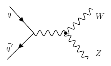
Figure 1: Feynman diagram for WZ production where effects of dimension-6 operators affecting the triple gauge boson vertex are shown.

A detailed measurement of this process is performed by both the ATLAS and CMS Collaborations using Run-2 LHC data [25, 26].

For the SM, the WZ process is generated at LO using Madgraph5 aMC@NLO v2.6.5 [17]. The NNPDF3.1 NNLO PDF set [27] is used. The renormalization and factorization scales chosen are half of the sum of the transverse mass of final state particles. The SMEFT effects are simulated at LO using the SMEFTsim v3.0 [28] model with the topU3l flavor scheme. Event samples are produced at both the SM point, i.e., setting all Wilson coefficients to zero and with non-zero values of Wilson coefficients for the operators considered. Several weights are stored for each event. Those are computed using reweighting for matrix element method [29] following two approaches: helicity-aware and -ignorant reweightings. Ten million events are generated for each of the samples separately with helicity-aware and -ignorant reweightings. For the generated samples, one million events are generated.

The WZ production at the SM is dominated by the helicity configuration where both the bosons are transversely polarized with opposite helicities ($\pm$,$\mp$), whereas the SMEFT operators considered here affect the configuration with both the bosons have the same transverse helicities ($\pm$,$\pm$) [30]. This is depicted in Fig. 2 as a function of W boson p${}_{\textrm{T}}$ using the event samples produced for this study.

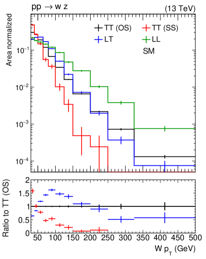
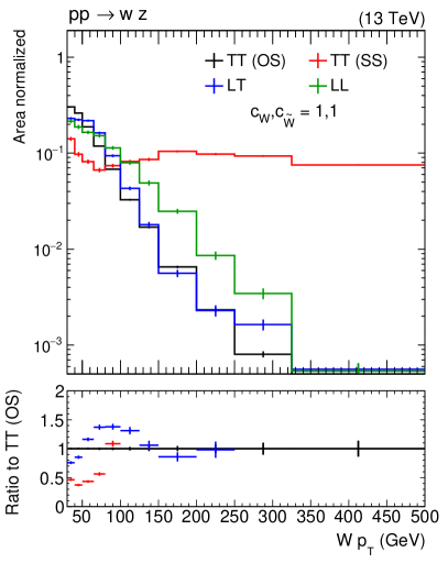
Figure 2: Helicity composition as a function of W boson p_T at the SM point (left) and a BSM point with both $c_{W}$ and $c_{\tilde{W}}$ set to 1 (right). Here, L and T refer to longitudinal and transverse polarizations, respectively, whereas OS and SS refer to the opposite- and same-sign configurations, respectively. The helicity eigenstates are defined in the laboratory reference frame.

Both the SMEFT operators modify the W boson p${}_{\textrm{T}}$ spectrum. So, it is used as an observable to compare between samples where the prediction at an EFT point is obtained using event weights and those produced directly at that particular EFT point, referred to as reweighted and generated predictions, respectively. The comparisons are shown in Fig. 3 for the case where $c_{W}$ and $c_{\tilde{W}}$ have a value of 1. The top row of Fig. 3 shows the comparison of W boson p${}_{\textrm{T}}$ spectra, summed over all possible helicity configurations, in reweighted and generated samples for two choices of the reference point in reweighting: SM point and a BSM point, where Wilson coefficients of both the operators are set to 0.5. For the SM reference point, the helicity-ignorant reweighting can reproduce the W boson p_T spectrum predicted by the generated sample except at very high-p_T values, where statistics is small, but the helicity-aware reweighting fails. Both helicity-aware and -ignorant reweightings model the generated W boson p${}_{\textrm{T}}$ spectra very well once the BSM reference point is used in reweighting. The bottom row of Fig. 3 shows the same comparison as the top row but specifically for the helicity configuration affected by the SMEFT operators. Here, it is evident that helicity-ignorant reweighting fails to model the p${}_{\textrm{T}}$ spectra for individual helicity configurations irrespective of the reference point chosen in reweighting, whereas the helicity-aware reweighting with a BSM reference point can model the W boson p${}_{\textrm{T}}$ spectrum for a specific helicity configuration, affected by the SMEFT operators considered.

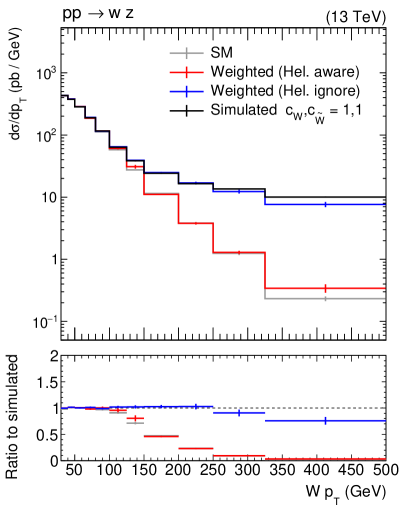
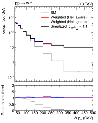
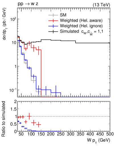
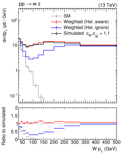
Figure 3: Comparison of W boson $p_{T}$ spectra between generated and reweighted (both helicity-aware and -ignorant variants) at a BSM point ($c_{W}$, $c_{\tilde{W}}$ = 1, 1) for two reference points used in the reweighting: the SM point (left) and a BSM point with both $c_{W}$ and $c_{\tilde{W}}$ set to 0.5 (right). The upper row corresponds to the case where all helicity configurations are summed, and the lower row corresponds to only the same-sign transverse polarization configuration.

5.2 Helicity and reweighting of predictions for the ZH process

In this section, we study the modeling of SMEFT effects in Higgs production in association with a W or a Z boson, referred to as VH production. This particular Higgs production mode is extremely important to look for the effects of new physics since its contribution becomes increasingly important at high values of Higgs boson p${}_{\textrm{T}}$ [31]. The VH process has been measured by both ATLAS and CMS Collaborations across different decay channels [32, 33]. The VH production is affected by a number of SMEFT operators at dimension 6 in the following ways:

• modifying the vector boson coupling to quarks or giving rise to a four-point interaction

• modifying the Higgs boson interaction with $\mathup{{{W}}}$ or $\mathup{{{Z}}}$ boson

For this study, we restrict ourselves to the ZH production only and focus on one vector coupling operator ${{\mathcal{O}}^{(3)}_{Hq}}$ and two HVV operators ${{\mathcal{O}}_{HW}}$ and ${{\mathcal{O}}_{H\tilde{W}}}$ that affect both WH and ZH productions. The final state with the Z boson decaying to the leptons and the Higgs boson decaying to a pair of b quarks, measured by both the ATLAS and CMS Collaborations [34, 35, 36], is considered. The ${{\mathcal{O}}^{(3)}_{Hq}}$ operator mainly affects the helicity configuration where the Z boson is longitudinally polarized, which is also dominant in the SM. The HVV operators, on the other hand, also affect the interference of scattering amplitudes with different helicities of Z boson that get reflected in the distribution of angles constructed using Higgs boson and leptons from Z boson [37] as depicted in Fig. 4.

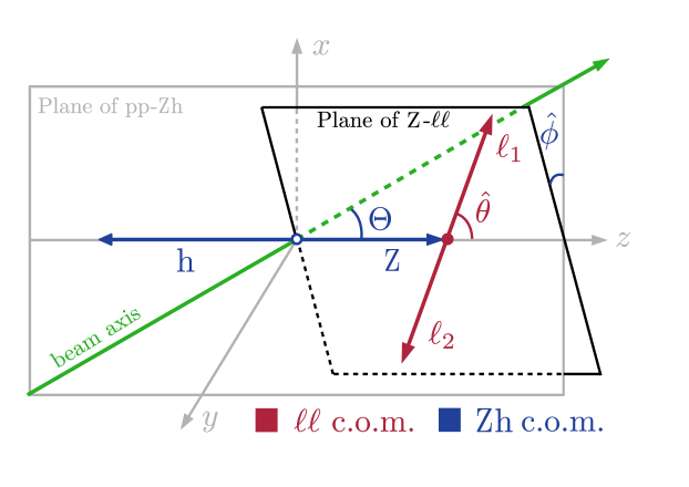
Figure 4: Decay planes and angles in the Z($\rightarrow$ l⁺l^- )H($\rightarrow$ b $\bar{\textrm{b}}$) production. The angle $\Theta$ and $\phi$ are defined in the ZH rest frame, while $\theta$ is defined in the Z boson rest frame.

The ZH production process followed by the leptonic decay of the Z boson and the Higgs boson decay to a pair of bottom quarks is generated at LO with up to one additional jet using Madgraph5 aMC@NLO v2.6.5 [17]. The NNPDF3.1 NNLO PDF set [27] is used. The renormalization and factorization scales chosen are half of the sum of the transverse mass of final state particles. The SMEFT effects are simulated at LO using the SMEFTsim v3.0 [28] model with the topU3l flavor scheme. For each event, several weights are stored, which are computed by ME reweighting [29] following two approaches: helicity-aware and -ignorant reweightings. The SM point, i.e. all Wilson coefficients set to 0, is used as the reference point in reweighting. Separate samples are produced by turning on one operator at a time with the following values: a) c${}_{Hq}^{(3)}$ = 0.1, b) c_HW = 1, c) c${}_{H\tilde{W}}$ = 1; in each case, values of all other Wilson coefficients are set to 0. These are referred to as the generated samples. One million events are generated for each of the reweighted and generated samples.

The particle-level Z boson p${}_{\textrm{T}}$ spectra predicted by reweighted samples are compared to the one from the generated samples as shown in Fig. 5. In this case, both helicity-aware and -ignorant variants of reweighting model the effects of ${{\mathcal{O}}^{(3)}_{Hq}}$ and ${{\mathcal{O}}_{HW}}$ on Z boson p${}_{\textrm{T}}$ well.

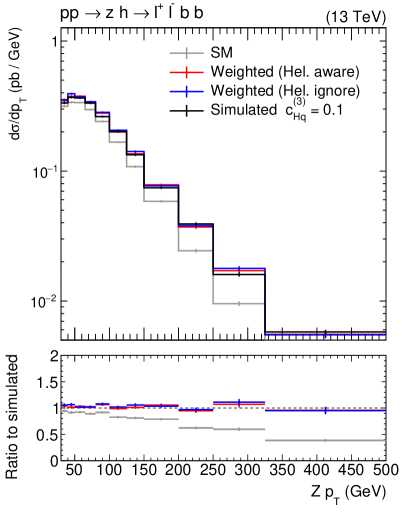
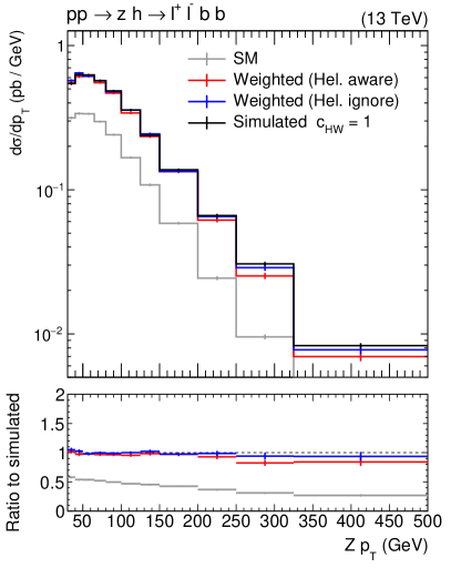
Figure 5: Comparison of Z boson p${}_{\textrm{T}}$ spectra (absolute cross section per GeV on the y-axis) between generated and reweighted (with both helicity-aware and -ignorant variants) ZH samples at c${}_{Hq}^{3}$=0.1 (left) and c_HW=1 (right). The helicity eigenstates are defined in the laboratory reference frame.

Next, we compare the distributions of angle $\theta$ and $\phi$ depicted in Fig. 4 between reweighted and generated samples in Fig. 6 for c_HW and c${}_{H\tilde{W}}$ separately. For both HVV operators, two variants of reweighting model the angular distributions obtained from the generated samples within statistical uncertainties. For the angle $\phi$, one can notice that it follows a $\cos{2\phi}$ distribution for c_HW=1, which is modified for c${}_{H\tilde{W}}$=1 due to different terms in the interference between scattering amplitudes being relevant for CP-even and -odd gauge coupling operators, respectively. Therefore, the variable $\phi$ can be used to probe the CP nature of Higgs to vector boson interaction.

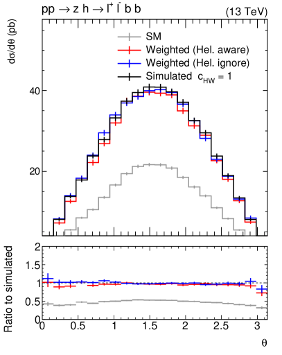
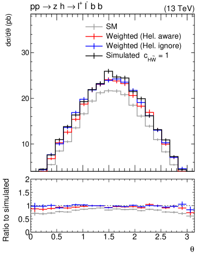
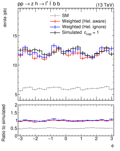
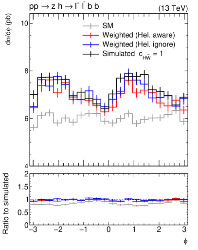
Figure 6: Comparison of $\theta$ (top) and $\phi$ (bottom) distributions (absolute cross section on the y-axis) between generated and reweighted (with both helicity-aware and -ignorant variants) ZH samples at c_HW=1 (left) and c${}_{H\tilde{W}}$=1(right). The angle $\phi$ is defined in the ZH rest frame, while $\theta$ is defined in the Z boson rest frame.

5.3 The $\textrm{t}\overline{\textrm{t}}$ process

In the SM, top-quark pair production ($\mathup{{{t}}}$$\mathup{{\overline{{{\mathup{{{t}}}}}}}}$) in proton-proton collisions proceeds predominantly via gluon-gluon fusion ($\sim 90\%$) followed by quark-antiquark annihilation ($\sim 10\%$) at LO. At NLO in QCD and beyond, channels with quark-gluon initial states appear. In this section, we aim to include all operators that significantly impact the $\mathup{{{t}}}$$\mathup{{\overline{{{\mathup{{{t}}}}}}}}$ processes. In Table 2, two-heavy-two-light four-quark operators are listed that can impact the $\mathup{{{t}}}$$\mathup{{\overline{{{\mathup{{{t}}}}}}}}$ process. In addition, the ${{{\mathcal{O}}^{(ij)}_{uG}}}$ operator from Table 1 affects the $\mathup{{{t}}}$$\mathup{{\overline{{{\mathup{{{t}}}}}}}}$ rate significantly. Therefore, both the real and imaginary parts of the WC for the ${{{\mathcal{O}}^{(ij)}_{uG}}}$ operator, ctGRe and ctGIm, are considered in this study. In this work, we only include those operators of the Warsaw basis that explicitly modify the couplings of the top quark with the other SM fields. We therefore do not include the ${{\mathcal{O}}_{G}}$ and ${{\mathcal{O}}_{\varphi G}}$ operators that are well constrained by processes that do not involve top quarks [38, 39].

The signal contribution is modeled at LO using the Madgraph5 aMC@NLO v2.6.5 event generator with the SMEFTsim model to incorporate the EFT effects. The definitions of the operators associated with all of these WCs are provided in [40]. As discussed in Sec. 1, the cross section (inclusive or differential) depends quadratically on the WCs. We have parameterised each event weight as a quadratic function of WCs, as described in Eq. 8, by including enough reweighting points per event. The nominal $\mathup{{{t}}}$$\mathup{{\overline{{{\mathup{{{t}}}}}}}}$ sample is generated at a starting point in the WC parameter space far from the SM point. The reference point of the nominal sample, called “LO (sample 1)”, is set to Pt1 as defined below. To simulate EFT impacts on the $\mathup{{{t}}}$$\mathup{{\overline{{{\mathup{{{t}}}}}}}}$ production from quark-gluon initial states and to predict distributions in the presence of extra jets more accurately, we produce another sample that includes an additional final-state parton in the matrix element generation. This sample is also produced at reference point Pt1, and is called "LO+1 jet (sample 1)". Both $\mathup{{{t}}}$$\mathup{{\overline{{{\mathup{{{t}}}}}}}}$ and $\mathup{{{t}}}$$\mathup{{\overline{{{\mathup{{{t}}}}}}}}$ +1jet samples include the dominant t $\rightarrow$ Wb decay followed with the leptonic decays of W boson.

It is important to make sure that the generated sample is able to be consistently reweighted to other points in EFT parameter space. In order to check that, we have generated independent $\mathup{{{t}}}$$\mathup{{\overline{{{\mathup{{{t}}}}}}}}$ samples at the following points in EFT space,

• SM point: all WCs set to zero.

• Dedicated point: All WCs set to zero except one which is set to -4,-2, 2, and 4 independently. The value of ctGRe is set to -0.4, -0.2, 0.2, 0.4 because of its large effect on the cross section.

• Pt1: WCs set to c${}_{\rm tG}^{Im}=0.7$, c${}_{\rm tG}^{Re}=0.7$, c${}_{\rm Qj}^{38}=9.0$, c${}_{\rm Qj}^{18}=7.0$, c${}_{\rm Qu}^{8}=9.5$, c${}_{\rm Qd}^{8}=12.0$, c${}_{\rm tj}^{8}=7.0$, c${}_{\rm tu}^{8}=9.0$, c${}_{\rm td}^{8}=12.4$, c${}_{\rm Qj}^{31}=3.0$, c${}_{\rm Qj}^{11}=4.2$, c${}_{\rm Qu}^{1}=5.5$, c${}_{\rm Qd}^{1}=7.0$, c${}_{\rm tj}^{1}=4.4$, c${}_{\rm tu}^{1}=5.4$, c${}_{\rm td}^{1}=7.0$

• Pt2: WCs set to c${}_{\rm tG}^{Im}=1.0$, c${}_{\rm tG}^{Re}=1.0$, c${}_{\rm Qj}^{38}=3.0$, c${}_{\rm Qj}^{18}=3.0$, c${}_{\rm Qu}^{8}=3.0$, c${}_{\rm Qd}^{8}=3.0$, c${}_{\rm tj}^{8}=3.0$, c${}_{\rm tu}^{8}=3.0$, c${}_{\rm td}^{8}=3.0$, c${}_{\rm Qj}^{31}=3.0$, c${}_{\rm Qj}^{11}=3.0$, c${}_{\rm Qu}^{1}=3.0$, c${}_{\rm Qd}^{1}=3.0$, c${}_{\rm tj}^{1}=3.0$, c${}_{\rm tu}^{1}=3.0$, c${}_{\rm td}^{1}=3.0$.

The samples produced at Pt2 are called "LO (sample 2)" and "LO+1jet (sample 2)". In Fig. 7 and Fig. 8, relative SMEFT contributions to the $\mathup{{{t}}}$$\mathup{{\overline{{{\mathup{{{t}}}}}}}}$ inclusive cross section are shown for individual WCs. In each plot the quadratic function extracted from LO (sample 1) and the LO (sample 2) are compared to the cross section ratios calculated at the dedicated points. In general, there is good agreement between the cross section ratio values predicted by reweighting and those calculated at the dedicated points in EFT space.

In addition to the inclusive cross section estimation, LO+1jet (sample 1) should be able to predict differential distributions of various kinematic variables at different points in EFT space. In Fig. 9, distributions of top quark $p_{T}$, leading lepton $p_{T}$, and $\Delta R$ between two leptons are shown for $\mathup{{{t}}}$$\mathup{{\overline{{{\mathup{{{t}}}}}}}}$ events with two leptons (electron or muon) with $p_{t}>20$ GeV and $|\eta|<2.5$, and at least two jets with $p_{t}>20$ GeV and $|\eta|<2.5$. In the left column, differential distributions are shown for LO+1jet (sample 1) and LO+1jet (sample 2) reweighted to the SM point. In the right column LO+1jet (sample 1) and LO+1jet (sample 2) are reweighted to Pt2, the starting point of the sample 2. These distributions show that our nominal sample is able to describe the $\mathup{{{t}}}$$\mathup{{\overline{{{\mathup{{{t}}}}}}}}$ differential distributions in different points in EFT space including the SM point.

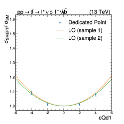
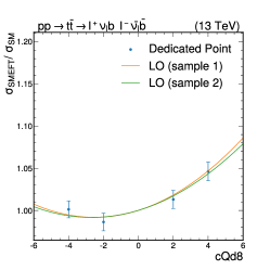
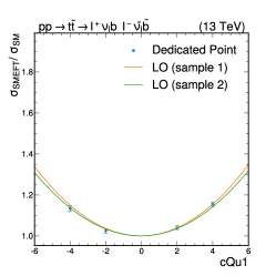
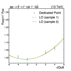
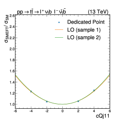
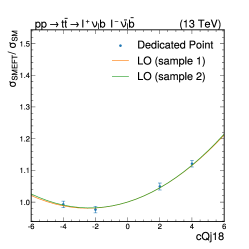
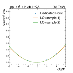
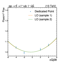
Figure 7: Relative modification of the $\mathup{{{t}}}$$\mathup{{\overline{{{\mathup{{{t}}}}}}}}$ total cross section, $\sigma_{\text{SMEFT}}/\sigma_{\text{SM}}$, induced by the presence of the SMEFT operators. Solid curves show the quadratic dependency of the relative cross section to the WC values obtained from reweighting sample 1 and sample 2 in EFT space. Blue points are obtained from dedicated simulations.

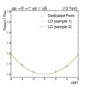
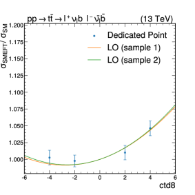
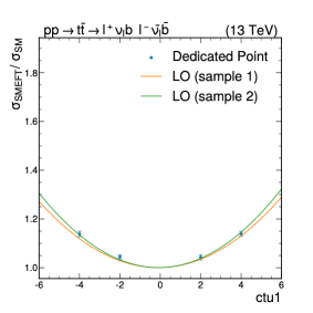
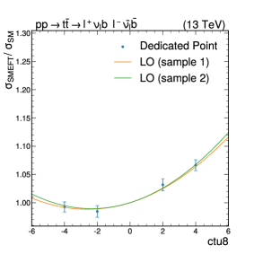
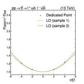
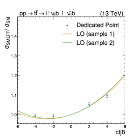
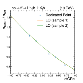
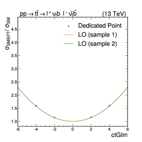
Figure 8: Relative modification of the $\mathup{{{t}}}$$\mathup{{\overline{{{\mathup{{{t}}}}}}}}$ total cross section, $\sigma_{\text{SMEFT}}/\sigma_{\text{SM}}$, induced by the presence of the SMEFT operators. Solid curves show the quadratic dependency of the relative cross section to the WC values obtained from reweighting sample 1 and sample 2 in EFT space. Blue points are obtained from dedicated simulations.

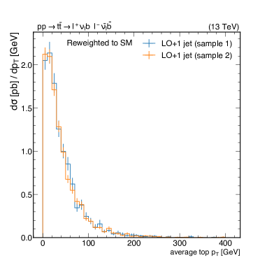
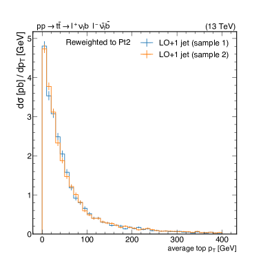
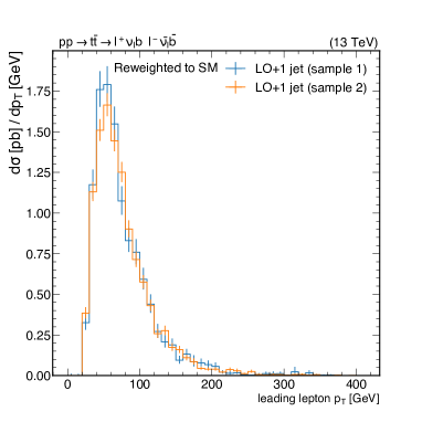
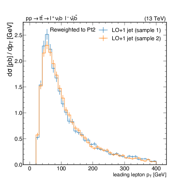
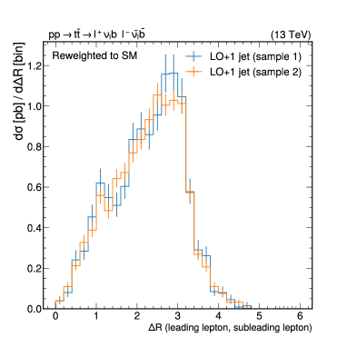
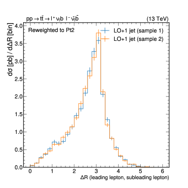
Figure 9: Differential distributions for $\mathup{{{t}}}$$\mathup{{\overline{{{\mathup{{{t}}}}}}}}$ +1jet process with respect to the top quark average $p_{T}$ (top), leading lepton $p_{T}$ (middle) and $\Delta R(\text{leading lepton, sub leading lepton})$ (bottom). Differential distributions obtained from reweighting both sample 1 and sample 2 to the SM point (left) and reweighting sample 1 to Pt2 (right).

5.4 Studies in the $\textrm{t}\overline{\textrm{t}}Z$ process at NLO

In this section, we analyze the EFT reweighting performance using as a benchmark process the production of a top-antitop pair in association with a Z boson emission, namely the $\textrm{t}\overline{\textrm{t}}\mathrm{Z}$ process. This process has been extensively studied both from ATLAS [41, 42] and CMS [43, 44], showing a high sensitivity to possible EFT effects coming from operators that modify the electroweak vertices. In this case, we focus on the ${{\mathcal{O}}_{tZ}}$ operator in Table 1, which modifies the interaction between the top quark and the Z boson.

To simulate the $\textrm{t}\overline{\textrm{t}}\mathrm{Z}$ process we use Madgraph5 aMC@NLO v2.6.5, while the EFT effects are taken into account using the SMEFTsim [28] and the SMEFT@NLO [45] models. The events are generated at NLO in QCD when using the SMEFT@NLO model and at LO plus an additional parton with the SMEFTsim model, while the parton shower is modeled using PYTHIA8[46]. For the generation of the LO samples, particular attention is dedicated to the matching procedure as discussed in Sec.4. Both simulations are performed in the 5 flavour scheme choosing as scale half of the sum of transverse masses. We generate events assuming the SM and assuming $c_{\textrm{tZ}}=1$ in the SMEFT@NLO convention. We then compare the definitions of the operator in the two models to set the corresponding value of $c_{\textrm{tZ}}$ in the LO simulation with the SMEFTsim model.

In Fig. 10 and Fig. 11, the distributions of the top quark and Z boson transverse momentum for the SM and the different EFT prediction generation strategies are shown. The left plot shows the distributions from the LO simulation while in the right one, the NLO results are presented. It is not possible to separate linear and quadratic EFT contributions in the NLO simulation in MG v2, so only the reweighted simulation and the separate simulation distributions are shown.

In the two central panels in Fig. 10 the ratio between the EFT distributions and the SM is shown, highlighting an increase in sensitivity to the EFT effects in the tail of the top quark transverse momentum distribution. In the bottom panels, the ratio among the different EFT generation strategies is presented, showing a good agreement along the whole spectrum.

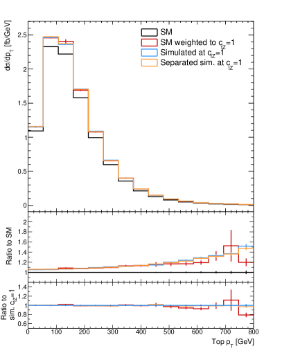
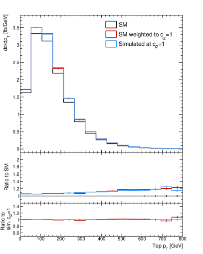
Figure 10: Top $p_{T}$ distribution simulated at LO + 1 jet (left) and at NLO (right). In black is depicted the SM distribution, while the other lines represent the different available simulation methods to compute EFT predictions. The first ratio plot highlights the sensitivity to the EFT effects. While, in the second ratio plot, the agreement between the direct simulation, the reweighted simulation, and the separate simulation (only for LO + 1 jet) is shown.

The Z boson transverse momentum distribution, in Fig. 11, shows a higher sensitivity to the EFT effect with respect to the top $p_{T}$ distribution. However, the agreement between the reweighted simulation and the other two EFT prediction strategies gets worse at high Z $p_{T}$ in the LO results. This arises from employing the helicity-aware reweighting using the SM as a reference point. In the NLO results, where only the helicity ignorant reweighting is possible, there remains a good agreement between the reweighted simulation and the direct simulation.

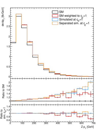
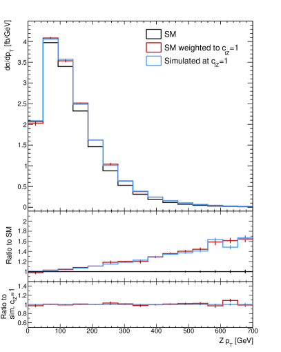
Figure 11: Z $p_{T}$ distribution simulated at LO + 1 jet (left) and at NLO (right). In black is depicted the SM distribution, while the other lines represent the different available simulation methods to compute EFT predictions. The first ratio plot highlights the sensitivity to the EFT effects. While, in the second ratio plot, the agreement between the direct simulation, the reweighted simulation, and the separate simulation (only for LO + 1 jet) is shown.

A downside of the reweighting simulation is the statistical fluctuations in poorly populated phase space due to large event weights. This is evident in Fig. 10 (left) and Fig. 11, where there are large statistical fluctuations in the reweighted distribution at high Z and top transverse momentum.

5.5 Helicity aware and ignorant reweighting in the $\textrm{t}\overline{\textrm{t}}Z$ process

In this section, we use the $\textrm{t}\overline{\textrm{t}}\mathrm{Z}$ process, which was already introduced in Sec. 5.4, to showcase the benefits and potential limitations of the helicity-ignorant reweighting approach. To do that, we generate $\textrm{t}\overline{\textrm{t}}\mathrm{Z}$ events using Madgraph5 aMC@NLO v2.6.7 and simulate EFT from the $\mathcal{O}_{\textrm{tZ}}$ operator from Table 1.

The $\mathcal{O}_{\textrm{tZ}}$ operator, defined as $-\sin\theta_{W}{{\mathcal{O}}_{uB}}+\cos\theta_{W}{{\mathcal{O}}_{uW}}$, introduces $\textrm{t}\overline{\textrm{t}}\mathrm{Z}$ vertices with helicity configurations that are not present in the SM and for this reason, the choice between helicity-ignorant and aware reweighting is particularly relevant. This is illustrated in Fig. 12, where we show the distribution of the spin of the different partons involved in $\textrm{t}\overline{\textrm{t}}\mathrm{Z}$ events. We consider events generated assuming the SM and assuming $c_{\textrm{tZ}}=5$. The figure also shows that certain helicity configurations that arise naturally in the BSM scenario are not present or suppressed in the SM. Because of this, it is not possible to use the helicity-aware method to reweight SM samples so that they reproduce this specific BSM scenario: the regions of the phase space spanned by these helicity configurations will not be populated by SM samples.

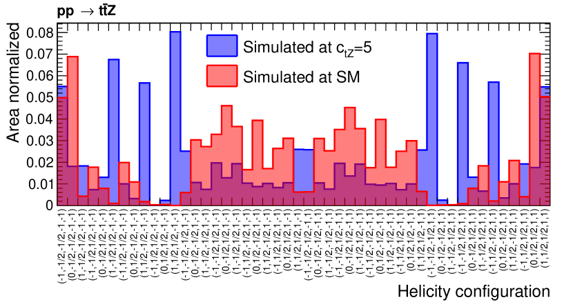
Figure 12: Distribution of the different helicity configurations in $\textrm{t}\overline{\textrm{t}}\mathrm{Z}$ generated at SM and $c_{\mathrm{tZ}}$=5 in the partonic center-of-mass frame. Bins of the distribution are labeled as $(h_{\mathrm{Z}},h_{\mathrm{t}},h_{\bar{\mathrm{t}}},h_{\mathrm{g}_{1}},h_{\mathrm{g}_{2}})$, where $h_{i}$ denotes the helicity of each particle. The distribution shows that some helicity configurations are not present at the SM and, therefore, helicity-aware reweighting cannot populate those regions of the phase space.

A consequence of this is shown in Fig. 13 where the inclusive $\textrm{t}\overline{\textrm{t}}\mathrm{Z}$ cross section dependence as a function of $c_{\textrm{tZ}}$ is shown. This dependence is computed using three independent samples with the same number of events. Two samples are generated assuming the SM and a third one is generated at $c_{\textrm{tZ}}=5$. The three samples are then weighted to $c_{\textrm{tZ}}=0,-1,1$ to obtain the inclusive $\textrm{t}\overline{\textrm{t}}\mathrm{Z}$ cross section for those values. From them, we interpolate the dependence using a second-order polynomial, whose coefficients are shown in Fig. 13. We take the $c_{\textrm{tZ}}=5$ as the reference value, which we expect to be more accurate since that one is expected to populate the full kinematic phase space. We use the helicity-aware and ignorant reweighting for each of the SM samples.

The trend predicted by the helicity-ignorant reweighting approach agrees with the one predicted by the reference value. In contrast, the helicity-aware predicts a significantly smaller quadratic term than the reference value and features larger statistical uncertainties than the other approaches. This is due to two reasons. On the one hand, the smaller value predicted by the helicity-aware approach is because it cannot populate phase space regions that are forbidden in the SM but present when $c_{\textrm{tZ}}\neq 0$. On the other hand, the larger uncertainties of this approach are due to a degradation of the statistical power of the weighted sample, which is due to large event weights arising from regions of the phase space that are suppressed but not forbidden in the SM. This shows two possible advantages of helicity-ignorant reweighting: it can be used to reweight SM samples to some BSM scenarios and, in addition, can be used in general to increase the statistical power of weighted samples.

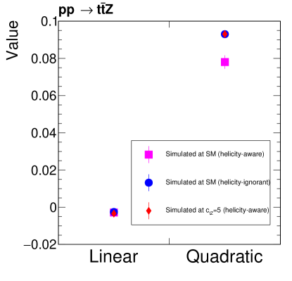
Figure 13: Quadratic parametrization of the $\textrm{t}\overline{\textrm{t}}\mathrm{Z}$ cross section as a function of $c_{\mathrm{tZ}}$ obtained by reweighting samples generated at the SM and $c_{\mathrm{tZ}}$=5 using the helicity-ignorant and aware methods.

Although the helicity-ignorant reweighting populates the kinematic phase space more efficiently, it gives rise to reweighted samples that do not necessarily reproduce the helicity configurations of the scenario that we are reweighting to. The helicity of the produced partons is not directly measurable but it can introduce correlations among the kinematics of the different final state particles. In analyses where these correlations are relevant keeping track of the helicity of the different particles is necessary.

To study this effect, we consider two different methods to model the decay of the produced partons. In both scenarios, we produce samples $c_{\textrm{tZ}}=5$ and reweight them to the SM and samples produced assuming the SM. In one of the scenarios, we use Madspin to model the decay of the top quarks and Z boson, and the weights are computed as a function of the top quarks and Z boson, before their decay. In the other scenario, the decay is modeled using Madgraph and the weights are computed as a function of the particles produced in the decay of the top quarks and Z boson. We note that, for this process, we only expect shortcomings due to the helicity-ignorant reweighting in the earlier scenario. In the latter scenario, the reweighting is performed as a function of the particles produced in the decay, and changes in their helicity do not give rise to observable effects.

In Fig. 14 we show the $\Delta\phi$ distribution between the two leptons produced in the Z boson decay. The plot shows that only the Madgraph decay model can produce consistent results, while Madspin is introducing artificial trends. These trends are present because Madspin computes and samples implicitly over $\mathcal{M}_{\mathrm{prod+decay}}/\mathcal{M}_{\mathrm{prod}}$, the ratio of the production+decay over production matrix elements, which is computed at the reference point. By default, Madspin does not recompute this ratio for reweighted events, so it introduces artificial trends when reweighting to a scenario for which $\mathcal{M}_{\mathrm{prod+decay}}/\mathcal{M}_{\mathrm{prod}}$ is different from the reference points.

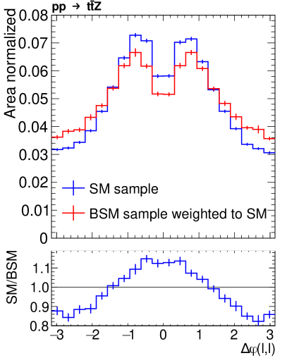
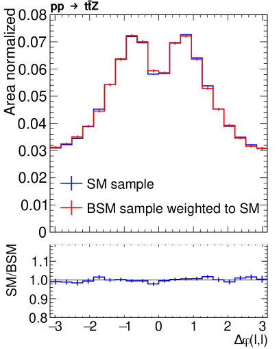
Figure 14: Distribution of the $\Delta\phi$ between the two leptons produced in the $\mathrm{Z}$ boson decay in samples where the top quarks and the $\mathrm{Z}$ boson have been decayed using Madspin (left) and the Madgraph decay syntax (right). Samples generated at the SM and $c_{\mathrm{tZ}}$=5 are both reweighted to the SM.

5.6 The VBF H process

Vector boson fusion (VBF) is one of the dominant Higgs boson production mechanisms at the LHC. This process has been measured by the ATLAS and CMS experiments in a variety of Higgs boson decay channels [32, 33]. These measurements rely on the presence of two forward (high $|\eta|$) quark-initiated jets to distinguish them from other H production modes.

Operators, including CP-odd ones, at dimension 6 in standard model effective field theory can modify the VBF process in a variety of ways by:

1. altering only the total cross section,

2. introducing anomalous couplings between the Higgs and vector bosons as shown in Fig. 15a,

3. introducing anomalous couplings between the quarks and vector bosons (Fig. 15b) or HVqq contact interactions (Fig. 15c).

Operators impacting Higgs boson decays are not considered.

Figure 15: Feynman diagrams representing VBF Higgs boson production with EFT contributions to (a) the HVV interaction, (b) the Vqq interaction, and (c) a VHqq contact interaction.

An SM VBF Higgs sample is generated at LO using Madgraph5 aMC@NLO v2.9.13 [17] and the NNPDF3.1 PDF set [47]. The renormalization and factorization scales are not kept fixed, and their values are the default in Madgraph5, namely the transverse mass of the $2\rightarrow 2$ system resulting from $k_{\text{T}}$ clustering. The SMEFTsim framework [28] is used with the topU3l model and $m_{W}$ input parameter scheme to provide per-event weights relative to the SM accounting for EFT contributions (both linear and quadratic) from each of the operators in Table 1. The EFT scale $\Lambda$ is chosen at 1 TeV, and Feynman diagrams with single-operator insertions are considered. The reweighting procedure used for this sample is helicity aware. Since the ${{\mathcal{O}}_{Hud}}$ operator induces a right-handed charged current, its effects are not captured in the simulated sample.

Five EFT scenarios are selected as representative examples of the three classes enumerated above $c_{H\Box}=1$, $c_{HW}=1$, $\tilde{c}_{HW}=1$, $c_{Hq^{(1)}}=1$, and $c_{Hq^{(3)}}=1$. In each case, only the listed Wilson coefficient is non-zero. In addition to the reweighted SM sample, each of these five EFT points is simulated directly up to quadratic order. For each EFT point, two additional samples are generated: one includes the linear term only, and the other includes the quadratic term only. The sum of the standard model, linear-only, and quadratic-only samples is expected to reproduce the full sample. The cross section of each EFT sample is listed in Table 3. Good agreement is observed between the various simulation methods.

Cross section [fb]	SM	$c_{H\Box}=1$	$c_{HW}=1$	$\tilde{c}_{HW}=1$	$c_{Hj^{(1)}}=1$	$c_{Hj^{(3)}}=1$
Reweighted	$-$	4.164	3.608	3.819	3.847	2.687
Direct sim.	3.675	4.140	3.618	3.829	3.859	2.778
SM + Lin. + Quad.	$-$	4.135	3.617	3.824	3.865	2.804

Table 3: VBF cross section calculated by Madgraph5 from one million simulated events.

Figure 16a shows the distribution of Higgs boson $p_{\textrm{T}}$ for the $c_{H\Box}=1$ scenario for each of the simulated samples. The overall cross section is enhanced with respect to the SM, as seen in Table 3. Note that the upper limit of the $p_{\textrm{T}}$ distribution (700 GeV) may be beyond the range of EFT validity. However, as this study is intended to validate the performance of different simulation strategies, the range of EFT validity is not considered. Figure 16b shows the angular separation $\Delta\eta$ between the spectator quarks in the event, which is similar in shape to the SM expectation.

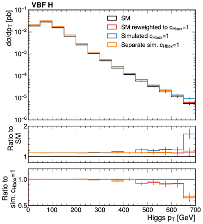
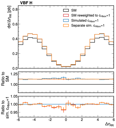
Figure 16: Distribution of (a) the Higgs boson $p_{T}$ and (b) the angular separation $\Delta\eta$ between the spectator quarks, for the $c_{H\Box}=1$ scenario. The SM expectation is shown in black. The prediction for $c_{H\Box}=1$ obtained by reweighting the SM point is shown in red. The direct simulation of $c_{H\Box}=1$ is shown in blue, and the sum of SM, linear-only, and quadratic-only is shown in orange. The middle panel shows the ratio to the SM, and the lower panel shows the ratio to the directly simulated sample.

Figure 17a shows the distribution of Higgs boson $p_{\textrm{T}}$ for the $c_{HW}=1$ scenario. Compared to the SM expectation, a deficit is observed below 50 GeV, and an enhancement is observed above about 150 GeV. Figure 17b shows the azimuthal separation $\Delta\phi$ between the spectator quarks for the $c_{HW}=1$ scenario. This distribution is strongly modified by the presence of the EFT operator: while the SM expectation shows that large angular separations are somewhat preferred, the distribution for $c_{HW}=1$ is nearly flat in this variable as the ${{\mathcal{O}}_{HW}}$ operator affects only the transverse amplitude $qV_{T}\rightarrow qH$ in VBF H production [48].

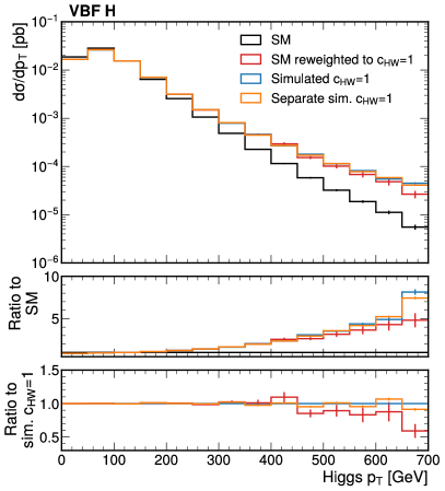
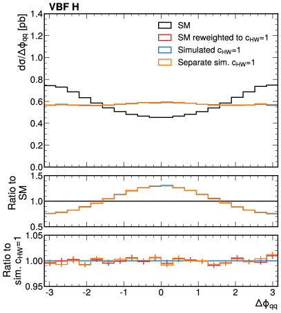
Figure 17: Distribution of (a) the Higgs boson $p_{T}$ and (b) the angular separation $\Delta\phi$ between the spectator quarks, for the $c_{HW}=1$ scenario. The SM expectation is shown in black. The prediction for $c_{HW}=1$ obtained by reweighting the SM point is shown in red. The direct simulation of $c_{HW}=1$ is shown in blue, and the sum of SM, linear-only, and quadratic-only is shown in orange. The middle panel shows the ratio to the SM, and the lower panel shows the ratio to the directly simulated sample.

Figure 18 shows the distribution of Higgs boson $p_{\textrm{T}}$ (a) and azimuthal separation $\Delta\phi$ between the spectator quarks (b) for the $\tilde{c}_{HW}=1$ scenario. Compared to the SM expectation, an enhancement in the $p_{\textrm{T}}$ is observed above about 150 GeV. The $\Delta\phi$ distribution is also slightly modified, though the effect is far weaker than that seen in Fig. 17b for the conjugate operator as the linear term, which models the interference between the SM and the EFT scenario, is small.

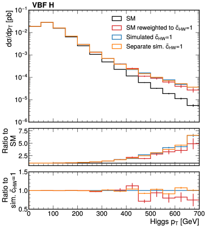
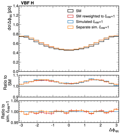
Figure 18: Distribution of (a) the Higgs boson $p_{T}$ and (b) the angular separation $\Delta\phi$ between the spectator quarks, for the $\tilde{c}_{HW}=1$ scenario. The SM expectation is shown in black. The prediction for $\tilde{c}_{HW}=1$ obtained by reweighting the SM point is shown in red. The direct simulation of $\tilde{c}_{HW}=1$ is shown in blue, and the sum of SM, linear-only, and quadratic-only is shown in orange. The middle panel shows the ratio to the SM, and the lower panel shows the ratio to the directly simulated sample.

Figure 19 shows the distribution of Higgs boson $p_{\textrm{T}}$ (a) and angular separation $\Delta\eta$ between the spectator quarks (b) for the $\tilde{c}_{Hj^{(1)}}=1$ scenario. Compared to the SM expectation, an enhancement in the $p_{\textrm{T}}$ is observed above about 150 GeV. It should be noted that the value of $\tilde{c}_{Hj^{(1)}}=1$ is large compared to existing constraints [49], but the large deviation with respect to the SM at high $p_{\textrm{T}}$ may fall outside the range of EFT validity. A small enhancement with respect to the SM is also seen for $|\Delta\eta|\sim 0$.

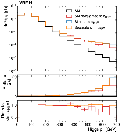
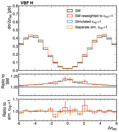
Figure 19: Distribution of (a) the Higgs boson $p_{T}$ and (b) the angular separation $\Delta\eta$ between the spectator quarks, for the $c_{Hj^{(1)}}=1$ scenario. The SM expectation is shown in black. The prediction for $c_{Hj^{(1)}}=1$ obtained by reweighting the SM point is shown in red. The direct simulation of $c_{Hj^{(1)}}=1$ is shown in blue, and the sum of SM, linear-only, and quadratic-only is shown in orange. The middle panel shows the ratio to the SM, and the lower panel shows the ratio to the directly simulated sample.

Figure 20 shows the distribution of Higgs boson $p_{\textrm{T}}$ (a) and angular separation $\Delta\eta$ between the spectator quarks (b) for the $\tilde{c}_{Hj^{(3)}}=1$ scenario. As for $\tilde{c}_{Hj^{(1)}}$, the value of $\tilde{c}_{Hj^{(3)}}=1$ is large compared to existing constraints [49]. Compared to the SM expectation, an overall lower cross section and a deficit in the range $100<p_{T}<300$ GeV is observed. A small deficit with respect to the SM is also seen for $|\Delta\eta|\sim 0$.

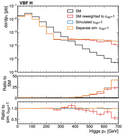
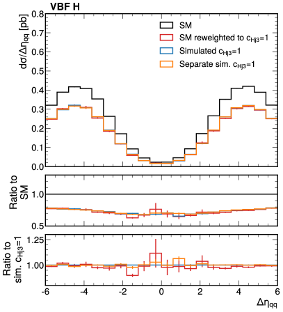
Figure 20: Distribution of (a) the Higgs boson $p_{T}$ and (b) the angular separation $\Delta\eta$ between the spectator quarks, for the $c_{Hj^{(3)}}=1$ scenario. The SM expectation is shown in black. The prediction for $c_{Hj^{(3)}}=1$ obtained by reweighting the SM point is shown in red. The direct simulation of $c_{Hj^{(3)}}=1$ is shown in blue, and the sum of SM, linear-only, and quadratic-only is shown in orange. The middle panel shows the ratio to the SM, and the lower panel shows the ratio to the directly simulated sample.

The comparison of these simulated EFT samples indicates good agreement between the predictions obtained by reweighting the SM prediction, directly simulating, and combining separately generated SM, linear, and quadratic components. In regions where the SM sample contains a limited number of events, such as at the highest $p_{\textrm{T}}$ and small $|\Delta\eta|$, some fluctuations and large uncertainties are observed in the reweighted spectrum.

5.7 Multiboson processes

5.7.1 Choice of dynamical scale

The dynamical scale, defined by certain functional forms, represents the factorization ($\mu_{\textrm{F}}$) and renormalization ($\mu_{\textrm{R}}$) scales. The following scale choices are implemented in Madgraph_aMC@NLO [50].

• Option 1: transverse mass of the $2\rightarrow 2$ system resulting of a $k_{\text{T}}$ clustering $\frac{1}{2}\sum_{i=1}^{N}\sqrt{m_{i}^{2}+p_{T,i}^{2}}$.

• Option 2: total transverse energy of the event $\sum_{i=1}^{N}\frac{E_{i}\cdot p_{T,i}}{\sqrt{p_{x,i}^{2}+p_{y,i}^{2}+p_{z,i}^{2}}}$.

• Option 3: sum of the transverse masses $\sum_{i=1}^{N}\sqrt{m_{i}^{2}+p_{T,i}^{2}}$.

• Option 4: half of the sum of the transverse masses $\frac{1}{2}\sum_{i=1}^{N}\sqrt{m_{i}^{2}+p_{T,i}^{2}}$.

• Option 5: partonic energy $\sqrt{\hat{s}}$.

The default scale choice is typically set to option 1 as defined above. This choice is insufficient for the generation of dimension-8 operators as shown in the left panel of Fig. 21. The dimension-8 operator under consideration is of the form shown in Eq. 20. However, the inadequacy of the choice of the default scale is independent of the exact choice of the operator.

$${\cal O}_{T,0}=Tr[\hat{W}_{\mu\nu}\hat{W}^{\mu\nu}]\times Tr[\hat{W}_{\alpha\beta}\hat{W}^{\alpha\beta}]$$ (20)

Each process in Fig. 21 is generated separately representing the SM-only (as a red-filled histogram), the interference between the SM and BSM components (as a green-filled histogram), and the BSM-only (as a blue-filled histogram) contribution. The exact syntax is given below (where the charge conjugate process was not generated in the interest of keeping the computation time low):

    - generate p p > w+ w+ w- T0=1 (for full generation, shown in black)
    - generate p p > w+ w+ w- (SM generation shown in red)
    - generate p p > w+ w+ w- T0^2==1
    (Interference between SM and BSM generation shown in green)
    - generate p p > w+ w+ w- T0^2==2 (BSM generation shown in blue)

The same syntax is used for both histograms on the left and the right. The only difference is the choice of the dynamical scale, where the total transverse energy in the event (Option 2 above) is used for the plot on the right panel of Fig. 21. The total transverse energy in the event is a superior choice for the generation of processes with the inclusion of dimension-8 operators in triboson processes in the bulk of the distribution (right panel of Fig 21), while the tail of the distribution is better predicted by the default choice of scale (left panel of Fig. 21). A possible reason for this behavior is that a single scale choice is not valid for processes that traverse a wide kinematic range. Therefore the a-priori expectation that the same value of the scale will be sufficient for both the SM process and the BSM process is flawed.

A similar effect is seen for vector boson scattering topologies as shown in Fig. 22. However in this case the distribution for the SM process is shown, where the SM distribution is obtained by reweighting a BSM distribution down to the SM scenario. Other factors that could impact the process generation non-negligibly such as the PDF are shown. In the ratio panel, the net effect of the variation of these parameters can be seen, pointing to the need to include these effects in analyses as possible sources of systematic uncertainty.

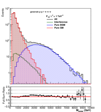
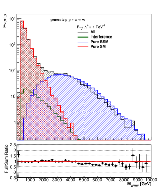
Figure 21: Impact of the choice of scale in a triboson process. The SM, BSM, and interference terms are generated separately and represented by the red, blue, and green hatch-filled histograms. The full process generated with all components of the generation is represented with a black hatch-filled histogram. The syntax of the full process is analogous to the process definition when the reweighting feature of Madgraph is used.

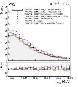
Figure 22: Impact of the choice of scale choice in a VBS process. The gray filled histogram is produced for a direct generation of the SM term as a $2\rightarrow 6$ or p p > e+ ve j j j j QCD=0 NP=0 SMHLOOP=0. The red, green, black, cyan and orange open histograms show the same process for various generator parameters such as the variation in the top width ($\Gamma_{t}$), different choice of the functional form of the dynamical scale and various PDFs. The magenta points show a further comparison with a $2\rightarrow 4$ or p p > v v j j QCD=0 NP=0 SMHLOOP=0 process [51].

5.8 Post-generation reweighting

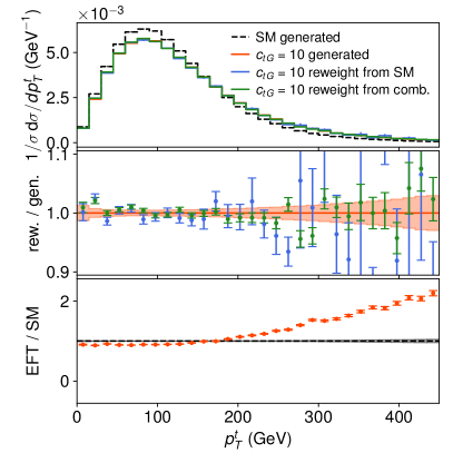
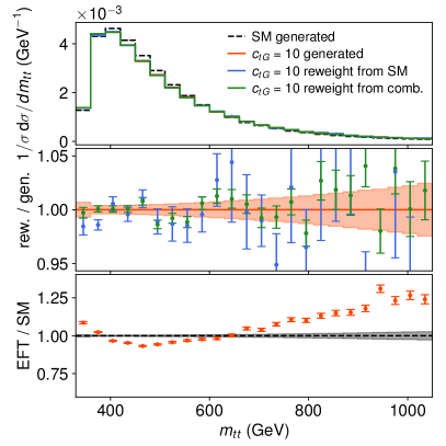
Figure 23: Top quark $p_{T}$ (left) and $m_{t\overline{t}}$ (right) for SM (black) and SMEFT with $c_{tG}=10$ for different production methods: Directly generated (orange), reweighted from an SM sample (blue) and reweighted from a combination of SM and other EFT samples (green). Both reweightings were performed after the sample generation. The panels show the normalized differential cross section (top), the ratio of two reweighting schemes to the direct generation (center), and the ratio of EFT and SM (bottom).

The procedure of reweighting events is often done by the same application that generated the events, and usually immediately after the generation, as part of a single execution of the application. This is how all of the previous studies shown in this report have been performed. This requires that the EFT model and desired Wilson coefficient values (EFT points) are defined at the time of sample generation. However, the need for a new model, or different EFT points, might arise after generation, and re-generating a sample can come with significant computing costs, especially when a full detector simulation is involved.

Though it is less common, it is possible to reweight events post-generation, thereby avoiding the significant computing costs associated with regeneration. In practice, this can be achieved by generating an external matrix element library from MadGraph 5. These libraries, which come in the format of a Python module, are specific to a particular model and set of reweighting points. If provided with the LHE-level information from the original generation, a new weight for each reweighting point can be provided by the module.

An advantage of the post-generation approach is that any UFO model can be used as long as the initial and final states of the process match that from the original generation, and the phase space is adequately covered. This makes it possible to reuse existing SM samples for an EFT analysis, leading to a (possibly) quick interpretation of a SM measurement. Alternatively, an existing EFT analysis could be easily reinterpreted with, for example, new flavor assumptions. Furthermore, these advantages are not limited to samples generated with MadGraph. As long as the LHE information is available, the reweighting module can be applied to events from any generator.

An example of post-generation reweighting is shown in Fig. 23 for $t\overline{t}$ production using the $c_{tG}$ Wilson coefficient in the dim6top model. First, a SM $t\overline{t}$ sample is reweighted post-generation to an EFT point with $c_{tG}=10$ (green), and compared to a direct generation of the same point (orange).

Going further, it is also possible to combine multiple reference samples, each reweighted independently to the same EFT point, into one large sample with higher statistics. This can also be used if the different reference samples cover different areas of the phase space (though care should be taken to remove very large-weight events). The green line in Fig. 23 shows an example where the reweighted SM $t\overline{t}$ sample was combined with reweighted EFT samples with original Wilson coefficient values of $c_{tG}=1$ and $c_{tG}=3$. The samples were combined by scaling the event weights of each sample by $\sum w/\sum w^{2}$, where the sums are over an individual sample, not the combination, and then concatenating the events. Given the reference samples used, this approach leads to the lowest statistical uncertainty in the inclusive sum of weights. In Fig. 23, one can see improved statistics in the combined sample compared to the reweighted SM sample, especially in the relevant high-energy tails of the distributions.

6 Summary

This note serves as a guide to strategies for obtaining simulation-based predictions in the context of SMEFT. It does not aim at establishing authoritative guidelines on how those predictions should be obtained but aims at assessing the consistency and computational efficacy.

We provide the statistical interpretation of simulation-based and weight-based strategies and discuss in some detail the intricacies related to the choice of the role of the helicity configuration in the reweighting. Common pitfalls and limitations of the methodology are discussed in Sec. 4 in the hope of alerting the unaware user.

In the main body of the note, we compare predictions for various final states. We study helicity-aware and ignorant reweighting in the WZ and ZH production process. In the top quark sector, pair production and associate production of a top quark pair and a Z boson are investigated. Good closure is observed in almost all the cases and for most of the considered kinematic phase space. The VBF production of an H boson and triboson processes complete the studies and lay the ground for future EFT measurements at the LHC.

References

- [1] W. Buchmuller and D. Wyler, Effective Lagrangian Analysis of New Interactions and Flavor Conservation, Nucl. Phys. B 268, 621 (1986), 10.1016/0550-3213(86)90262-2.
- [2] C. N. Leung, S. T. Love and S. Rao, Low-Energy Manifestations of a New Interaction Scale: Operator Analysis, Z. Phys. C 31, 433 (1986), 10.1007/BF01588041.
- [3] C. Degrande, N. Greiner, W. Kilian, O. Mattelaer, H. Mebane, T. Stelzer, S. Willenbrock and C. Zhang, Effective Field Theory: A Modern Approach to Anomalous Couplings, Annals Phys. 335, 21 (2013), 10.1016/j.aop.2013.04.016, 1205.4231.
- [4] I. Brivio and M. Trott, The Standard Model as an Effective Field Theory, Phys. Rept. 793, 1 (2019), 10.1016/j.physrep.2018.11.002, 1706.08945.
- [5] G. Isidori, F. Wilsch and D. Wyler, The standard model effective field theory at work, Rev. Mod. Phys. 96(1), 015006 (2024), 10.1103/RevModPhys.96.015006, 2303.16922.
- [6] S. Dawson et al., Precision matching of microscopic physics to the Standard Model Effective Field Theory (SMEFT), LHC EFT WG note (2022), 2212.02905.
- [7] N. Castro, K. S. Cranmer, A. Gritsan, J. W. Howarth, G. Magni, K. Mimasu, J. Rojo Chacon, J. Roskes, E. Vryonidou and T.-T. You, Experimental Measurements and Observables, LHC EFT WG note (2022), 2211.08353.
- [8] I. Brivio et al., Truncation, validity, uncertainties, LHC EFT WG note (2022), 2201.04974.
- [9] J. Brehmer, K. Cranmer, G. Louppe and J. Pavez, A guide to constraining effective field theories with machine learning, Phys. Rev. D 98, 052004 (2018), 10.1103/PhysRevD.98.052004, 1805.00020.
- [10] S. Chen, A. Glioti, G. Panico and A. Wulzer, Boosting likelihood learning with event reweighting, JHEP 03, 117 (2024), 10.1007/JHEP03(2024)117, 2308.05704.
- [11] S. Chatterjee, S. Rohshap, R. Schöfbeck and D. Schwarz, Learning the EFT likelihood with tree boosting (2022), 2205.12976.
- [12] S. Chatterjee, N. Frohner, L. Lechner, R. Schöfbeck and D. Schwarz, Tree boosting for learning EFT parameters, Comput. Phys. Commun. 277, 108385 (2022), 10.1016/j.cpc.2022.108385, 2107.10859.
- [13] K. Cranmer, J. Pavez and G. Louppe, Approximating likelihood ratios with calibrated discriminative classifiers, (2015), 1506.02169.
- [14] J. Brehmer, K. Cranmer, G. Louppe and J. Pavez, Constraining effective field theories with machine learning, Phys. Rev. Lett. 121, 111801 (2018), 10.1103/PhysRevLett.121.111801, 1805.00013.
- [15] J. Brehmer, G. Louppe, J. Pavez and K. Cranmer, Mining gold from implicit models to improve likelihood-free inference, Proc. Nat. Acad. Sci. 117, 5242 (2020), 10.1073/pnas.1915980117, 1805.12244.
- [16] J. Brehmer, F. Kling, I. Espejo and K. Cranmer, MadMiner: Machine learning-based inference for particle physics, Comput. Softw. Big Sci. 4, 3 (2020), 10.1007/s41781-020-0035-2, 1907.10621.
- [17] J. Alwall, R. Frederix, S. Frixione, V. Hirschi, F. Maltoni, O. Mattelaer, H. S. Shao, T. Stelzer, P. Torrielli and M. Zaro, The automated computation of tree-level and next-to-leading order differential cross sections, and their matching to parton shower simulations, JHEP 07, 079 (2014), 10.1007/JHEP07(2014)079, 1405.0301.
- [18] L. Lonnblad, Correcting the color dipole cascade model with fixed order matrix elements, JHEP 05, 046 (2002), 10.1088/1126-6708/2002/05/046, hep-ph/0112284.
- [19] R. Goldouzian, J. H. Kim, K. Lannon, A. Martin, K. Mohrman and A. Wightman, Matching in jet SMEFT studies, JHEP 06, 151 (2021), 10.1007/JHEP06(2021)151, 2012.06872.
- [20] J. Alwall et al., Comparative study of various algorithms for the merging of parton showers and matrix elements in hadronic collisions, Eur. Phys. J. C 53, 473 (2008), 10.1140/epjc/s10052-007-0490-5, 0706.2569.
- [21] J. Alwall, S. de Visscher and F. Maltoni, QCD radiation in the production of heavy colored particles at the LHC, JHEP 02, 017 (2009), 10.1088/1126-6708/2009/02/017, 0810.5350.
- [22] P. Lenzi and J. M. Butterworth, A Study on Matrix Element corrections in inclusive Z/ gamma* production at LHC as implemented in PYTHIA, HERWIG, ALPGEN and SHERPA (2009), 0903.3918.
- [23] C. Englert, M. Russell and C. D. White, Effective Field Theory in the top sector: do multijets help?, Phys. Rev. D 99(3), 035019 (2019), 10.1103/PhysRevD.99.035019, 1809.09744.
- [24] B. Grzadkowski, M. Iskrzynski, M. Misiak and J. Rosiek, Dimension-Six Terms in the Standard Model Lagrangian, JHEP 10, 085 (2010), 10.1007/JHEP10(2010)085, 1008.4884.
- [25] ATLAS collaboration, Measurement of production cross sections and gauge boson polarisation in collisions at TeV with the ATLAS detector, Eur. Phys. J. C 79(6), 535 (2019), 10.1140/epjc/s10052-019-7027-6, 1902.05759.
- [26] CMS collaboration, Measurement of the inclusive and differential WZ production cross sections, polarization angles, and triple gauge couplings in pp collisions at = 13 TeV, JHEP 07, 032 (2022), 10.1007/JHEP07(2022)032, 2110.11231.
- [27] R. D. Ball et al., Parton distributions from high-precision collider data, Eur. Phys. J. C 77(10), 663 (2017), 10.1140/epjc/s10052-017-5199-5, 1706.00428.
- [28] I. Brivio, Smeftsim 3.0 — a practical guide, Journal of High Energy Physics 2021(4) (2021), 10.1007/jhep04(2021)073.
- [29] P. Artoisenet, V. Lemaitre, F. Maltoni and O. Mattelaer, Automation of the matrix element reweighting method, JHEP 12, 068 (2010), 10.1007/JHEP12(2010)068, 1007.3300.
- [30] A. Azatov, J. Elias-Miro, Y. Reyimuaji and E. Venturini, Novel measurements of anomalous triple gauge couplings for the LHC, JHEP 10, 027 (2017), 10.1007/JHEP10(2017)027, 1707.08060.
- [31] K. Becker et al., Precise predictions for boosted Higgs production, SciPost Phys. Core 7, 001 (2024), 10.21468/SciPostPhysCore.7.1.001, 2005.07762.
- [32] CMS collaboration, A portrait of the Higgs boson by the CMS experiment ten years after the discovery, Nature 607, 60 (2022), 10.1038/s41586-022-04892-x, 2207.00043.
- [33] ATLAS collaboration, A detailed map of Higgs boson interactions by the ATLAS experiment ten years after the discovery, Nature 607, 52 (2022), 10.1038/s41586-022-04893-w, 2207.00092.
- [34] ATLAS collaboration, Measurements of and production in the decay channel in collisions at 13 TeV with the ATLAS detector, Eur. Phys. J. C 81(2), 178 (2021), 10.1140/epjc/s10052-020-08677-2, 2007.02873.
- [35] ATLAS collaboration, Measurement of the associated production of a Higgs boson decaying into -quarks with a vector boson at high transverse momentum in collisions at TeV with the ATLAS detector, Phys. Lett. B 816, 136204 (2021), 10.1016/j.physletb.2021.136204, 2008.02508.
- [36] CMS collaboration, Measurement of simplified template cross sections of the Higgs boson produced in association with W or Z bosons in the H→bb¯ decay channel in proton-proton collisions at s=13 TeV, Phys. Rev. D 109(9), 092011 (2024), 10.1103/PhysRevD.109.092011, 2312.07562.
- [37] S. Banerjee, R. S. Gupta, J. Y. Reiness, S. Seth and M. Spannowsky, Towards the ultimate differential SMEFT analysis, JHEP 09, 170 (2020), 10.1007/JHEP09(2020)170, 1912.07628.
- [38] F. Maltoni, E. Vryonidou and C. Zhang, Higgs production in association with a top-antitop pair in the Standard Model Effective Field Theory at NLO in QCD, JHEP 10, 123 (2016), 10.1007/JHEP10(2016)123, 1607.05330.
- [39] R. Goldouzian and M. D. Hildreth, LHC dijet angular distributions as a probe for the dimension-six triple gluon vertex, Phys. Lett. B 811, 135889 (2020), 10.1016/j.physletb.2020.135889, 2001.02736.
- [40] I. Brivio, SMEFTsim 3.0 — a practical guide, JHEP 04, 073 (2021), 10.1007/JHEP04(2021)073, 2012.11343.
- [41] ATLAS collaboration, Inclusive and differential cross-section measurements of production in collisions at TeV with the ATLAS detector, including EFT and spin-correlation interpretations (2023), 2312.04450.
- [42] ATLAS collaboration, Measurement of the and cross sections in proton-proton collisions at TeV with the ATLAS detector, Physical Review D 99(7), 072009 (2019), 10.1103/physrevd.99.072009.
- [43] CMS collaboration, Measurement of top quark pair production in association with a Z boson in proton-proton collisions at TeV, Journal of High Energy Physics 2020(3), 1 (2020), 10.1007/jhep03(2020)056.
- [44] CMS collaboration, Probing effective field theory operators in the associated production of top quarks with a Z boson in multilepton final states at TeV, Journal of High Energy Physics 2021(12) (2021), 10.1007/jhep12(2021)083.
- [45] C. Degrande, G. Durieux, F. Maltoni, K. Mimasu, E. Vryonidou and C. Zhang, Automated one-loop computations in the standard model effective field theory, Physical Review D 103(9) (2021), 10.1103/physrevd.103.096024.
- [46] T. Sjöstrand, S. Ask, J. R. Christiansen, R. Corke, N. Desai, P. Ilten, S. Mrenna, S. Prestel, C. O. Rasmussen and P. Z. Skands, An introduction to PYTHIA 8.2, Computer Physics Communications 191, 159–177 (2015), 10.1016/j.cpc.2015.01.024.
- [47] R. D. Ball et al., Parton distributions from high-precision collider data, Eur. Phys. J. C 77, 663 (2017), 10.1140/epjc/s10052-017-5199-5, 1706.00428.
- [48] J. Y. Araz, S. Banerjee, R. S. Gupta and M. Spannowsky, Precision SMEFT bounds from the VBF Higgs at high transverse momentum, JHEP 04, 125 (2021), 10.1007/JHEP04(2021)125, 2011.03555.
- [49] ATLAS collaboration, Interpretations of the ATLAS measurements of Higgs boson production and decay rates and differential cross-sections in collisions at TeV, http://cds.cern.ch/record/2870216 (2023).
- [50] V. Hirschi and O. Mattelaer, Automated event generation for loop-induced processes, JHEP 10, 146 (2015), 10.1007/JHEP10(2015)146, 1507.00020.
- [51] G. Boldrini, SM and EFT interpretation of Vector Boson Scattering measurements at CMS and development of the DAQ system for the Barrel Timing Layer for HL-LHC (PhD thesis), https://cds.cern.ch/record/2887923 (2024).