CERN-PH-TH/2007-066
LU-TP 07-13
KA-TP-06-2007
DCPT/07/62
IPPP/07/31
SLAC-PUB-12604
Comparative study of various algorithms for the merging of parton showers and matrix elements in hadronic collisions ***Work supported in part by the Marie Curie RTN “MCnet” (contract number MRTN-CT-2006-035606) and “HEPTOOLS” (contract number MRTN-CT-2006-035505).
J. Alwall1, S. Höche2, F. Krauss2, N. Lavesson3, L. Lönnblad3, F. Maltoni4, M.L. Mangano5, M. Moretti6, C.G. Papadopoulos7, F. Piccinini8, S. Schumann9, M. Treccani6, J. Winter9, M. Worek10,11
1 SLAC, USA;
2 IPPP, Durham, UK;
3 Department of Theoretical Physics, Lund University,
Sweden;
4 Centre for Particle Physics and Phenomenology (CP3)
Université Catholique de Louvain, Belgium;
5 CERN, Geneva, Switzerland;
6 Dipartimento di Fisica and INFN, Ferrara, Italy;
7 Institute of Nuclear Physics, NCSR Demokritos, Athens, Greece;
8 INFN, Pavia, Italy;
9 Institut für Theoretische Physik, TU Dresden,
Germany;
10 ITP, Karlsruhe University, Karlsruhe, Germany;
11 Institute of Physics, University of Silesia, Katowice, Poland.
We compare different procedures for combining fixed-order tree-level matrix-element generators with parton showers. We use the case of W-production at the Tevatron and the LHC to compare different implementations of the so-called CKKW and MLM schemes using different matrix-element generators and different parton cascades. We find that although similar results are obtained in all cases, there are important differences.
1 Introduction
One of the most striking features of LHC final states will be the large number of events with several hard jets. Final states with 6 jets from decays will have a rate of almost 1 Hz, with 10-100 times more coming from prompt QCD processes. The immense amount of available phase space, and the large acceptance of the detectors, with calorimeters covering a region of almost 10 units of pseudo-rapidity (), will lead to production and identification of final states with 10 or more jets. These events will hide or strongly modify all possible signals of new physics, which involve the chain decay of heavy coloured particles, such as squarks, gluinos or the heavier partners of the top, which appear in little-Higgs models. Being able to predict their features is therefore essential.
To achieve this, our calculations need to describe as accurately as possible both the full matrix elements for the underlying hard processes, as well as the subsequent development of the hard partons into jets of hadrons. However, for the complex final-state topologies we are interested in, no factorization theorem exists to rigorously separate these two components. The main obstacle is the existence of several hard scales, like the jet transverse energies and di-jet invariant masses, which for a generic multi-jet event will span a wide range. This makes it difficult to unambiguously separate the components of the event, which belong to the “hard process” (to be calculated using a multi-parton amplitude) from those developing during its evolution (described by the parton shower). A given -jet event can be obtained in two ways: from the collinear/soft-radiation evolution of an appropriate -parton final state, or from an -parton configuration where hard, large-angle emission during its evolution leads to the extra jet. A factorization prescription (in this context this is often called a “matching scheme” or “merging scheme”) defines, on an event-by-event basis, which of the two paths should be followed. The primary goal of a merging scheme is therefore to avoid double counting (by preventing some events to appear twice, once for each path), as well as dead regions (by ensuring that each configuration is generated by at least one of the allowed paths). Furthermore, a good merging scheme will optimize the choice of the path, using the one, which guarantees the best possible approximation to a given kinematics. It is possible to consider therefore different merging schemes, all avoiding the double counting and dead regions, but leading to different results in view of the different ways the calculation is distributed between the matrix element and the shower evolution. As in any factorization scheme, the physics is independent of the separation between phases only if we have complete control over the perturbative expansion. Otherwise a residual scheme-dependence is left. Exploring different merging schemes is therefore crucial to assess the systematic uncertainties of multi-jet calculations.
In this work we present a comprehensive comparison, for plus multijet production, of three merging approaches: the CKKW scheme, the Lönnblad scheme, and the MLM scheme. Our investigation is an evolution and extension of the work in [1], where Mrenna and Richardson presented implementations of CKKW for H ERWIG and the so-called pseudo-shower alternative to CKKW using P YTHIA , as well as the results of an approach inspired by the MLM-scheme. Our work considers the predictions of five different codes, A LPGEN , A RIADNE , H ELAC , M AD E VENT and S HERPA . A LPGEN implements the MLM scheme, and the results shown here are obtained with the H ERWIG shower; A RIADNE the Lönnblad scheme; H ELAC the MLM scheme, but will show results with the P YTHIA shower; M AD E VENT uses a variant of the MLM scheme, based on the CKKW parametrization of the multiparton phase-space; S HERPA , finally, implements the CKKW scheme. This list of codes therefore covers a broad spectrum of alternative approaches and, in particular, includes all the programs used as reference event generators for multijet production by the Tevatron and LHC experimental collaborations; for those, we show results relative to publically available versions, therefore providing valuable information on the systematics involved in the generation of multijet configurations by the experiments. A preliminary study, limited to the A LPGEN , A RIADNE and S HERPA codes, was presented in [2].
While [1] devoted a large effort to discussing the internal consistency and validation of the meging schemes, we refer for these more technical aspects to the papers documenting the individual implementations of the meging algorithms in the codes we use [3, 4, 5, 6, 7], and we shall limit ourselves here to a short review of each implementation. We concentrate instead on comparisons among physical observables, such as cross sections or jet distributions, which we study for both the Tevatron and the LHC. The main goal is not an anatomy of the origin of possible differences, but rather the illustration of their features and their size, to provide the experimentalists with a quantitative picture of systematics associated to the use of these codes. We furthermore verify that, with only a few noteworthy exceptions, the differences among the results of the various codes are comparable in size with the intrinsic systematics of each approach, and therefore consistent with a leading-logarithmic level of accuracy. The quantaties we present correspond to experimental observables and the differences between the predictions of the various codes that we present could therefore be resolved by comparing with data.
We begin the paper with a short review of the merging prescriptions and of their implementations in the 5 codes. We then introduce the observables considered for this study, and present detailed numerical results for both the Tevatron and the LHC. We then provide with an assessment of the individual systematics of each code, and a general discusison of our findings.
2 Merging procedures
In general, the different merging procedures follow a similar strategy:
-
1.
A jet measure is defined and all relevant cross sections including jets are calculated for the process under consideration. I.e. for the production of a final state in -collisions, the cross sections for the processes with are evaluated.
-
2.
Hard parton samples are produced with a probability proportional to the respective total cross section, in a corresponding kinematic configuration following the matrix element.
-
3.
The individual configurations are accepted or rejected with a dynamical, kinematics-dependent probability that includes both effects of running coupling constants and of Sudakov form factors. In case the event is rejected, step 2 is repeated, i.e. a new parton sample is selected, possibly with a new number of jets.
-
4.
The parton shower is invoked with suitable initial conditions for each of the legs. In some cases, like, e.g. in the MLM procedure described below, this step is performed together with the step before, i.e. the acceptance/rejection of the jet configuration. In all cases the parton shower is constrained not to produce any extra jet; stated in other words: configurations that would fall into the realm of matrix elements with a higher jet multiplicity are vetoed in the parton shower step.
The merging procedures discussed below differ mainly
-
•
in the jet definition used in the matrix elements;
-
•
in the way the acceptance/rejection of jet configurations stemming from the matrix element is performed;
-
•
and in details concerning the starting conditions of and the jet vetoing inside the parton showering.
2.1 CKKW
The merging prescription proposed in [8, 9] is known as the CKKW scheme and has been implemented in the event generator S HERPA [10] in full generality [11].
In this scheme
- •
-
•
the acceptance/rejection of jet configurations proceeds through a reweighting of the matrix elements with analytical Sudakov form factors and factors due to different scales in ;
-
•
the starting scale for the parton shower evolution of each parton is given by the scale where it appeared first;
-
•
a vetoed parton-shower algorithm is used to guarantee that no unwanted hard jets are produced during jet evolution.
In the original paper dealing with annihilations into hadrons, [8], it has been shown explicitly that in this approach the dependence on cancels to NLL accuracy. This can be achieved by combining the Sudakov-reweigthed matrix elements with a vetoed parton shower with angular ordering, subjected to appropriate starting conditions. The algorithm for the case of hadron–hadron collisions has been constructed in analogy to the case. However, it should be stressed that it has not been shown that the CKKW algorithm is correct at any logarithmic order in this kind of process.
For hadron-hadron collisions, the internal jet identification of the S HERPA -merging approach proceeds through a -scheme, which defines two final-state particles to belong to two different jets, if their relative transverse momentum squared
| (1) |
is larger than the critical value . In addition, the transverse momentum of each jet has to be larger than the merging scale . The magnitude , which is of order , is a parameter of the jet algorithm [15]. In order to completely rely on matrix elements for jet production allowed by the external analysis, the internal should be chosen less than or equal to the -parameter or, in case of a cone-jet algorithm, the -parameter employed by the external analysis.
The weight attached to the generated matrix elements consists of two components, a strong-coupling weight and an analytical Sudakov form-factor weight. For their determination, a -jet clustering algorithm guided by only physically allowed parton combinations is applied on the initial matrix-element configurations. The identified nodal -values are taken as scales in the strong-coupling constants and replace the predefined choice in the initial generation. The Sudakov weight attached to the matrix elements accounts for having no further radiation resolveable at . The NLL-Sudakov form factors employed, cf. [12], are defined by
| (2) |
where are the integrated splitting functions , and , which are given through
| (3) | |||||
| (4) | |||||
| (5) |
They contain the running coupling constant and the two leading, logarithmically enhanced terms in the limit . The single logarithmic terms and may spoil an interpretation of the NLL-Sudakov form factor as a non-branching probability. Therefore, is cut off at zero, such that retains its property to define the probability for having no emission resolvable at scale during the evolution from to . These factors are used to reweight in accordance to the appearance of external parton lines. A ratio of two Sudakov form factors accounts for the probability of having no emission resolvable at during the evolution from to . Hence, it is employed for the reweighting according to internal parton lines. The lower limit is taken to be or for partons that are clustered to a beam or to another final state parton, respectively.
The sequence of clusterings, stopped after the eventual identification of a configuration (the core process), is used to reweight the matrix element. Moreover, this also gives a shower history, whereas the core process defines the starting conditions for the vetoed shower. For the example of an identified pure QCD core process, the four parton lines left as a result of the completed clustering will start their evolution at the corresponding hard scale. Subsequently, additional radiation is emitted from each leg by evolving under the constraint that any emission harder than the separation cut is vetoed. The starting scale of each leg is given by the invariant mass of the mother parton belonging to the identified QCD splitting, through which the considered parton has been initially formed.
Finally, it should be noted that the algorithm implemented in S HERPA does the merging of the sequence of processes with fully automatically – the user is not required to generate the samples separately and mix them by hand.
2.2 The Dipole Cascade and CKKW
The merging prescription developed for the dipole cascade in the A RIADNE program[16] is similar to CKKW, but differs in the way the shower history is constructed, and in the way the Sudakov form factors are calculated. Also, since the A RIADNE cascade is ordered in transverse momentum the treatment of starting scales is simplified. Before going into details of the merging prescription, it is useful to describe some details of the dipole cascade, since it is quite different from conventional parton showers.
The dipole model[17, 18] as implemented in the A RIADNE program is based around iterating partonic splittings instead of the usual partonic splittings in a conventional parton shower. Gluon emission is modeled as coherent radiation from colour–anti-colour charged parton pairs. This has the advantage of eg. including first order corrections to the matrix elements for in a natural way and it also automatically includes the coherence effects modeled by angular ordering in conventional showers. The process of quark–anti-quark production does not come in as naturally, but can be added[19]. The emissions in the dipole cascade are ordered according to an invariant transverse momentum defined as
| (6) |
where is the squared invariant mass of parton and , with the emitted parton having index 2.
When applied to hadronic collisions, the dipole model does not separate between initial- and final-state gluon radiation. Instead all gluon emissions are treated as coming from final-state dipoles[20, 21]. To be able to extend the dipole model to hadron collisions, spatially extended coloured objects are introduced to model the hadron remnants. Dipoles involving hadron remnants are treated in a similar manner to the normal final-state dipoles. However, since the hadron remnant is considered to be an extended object, emissions with small wavelength are suppressed. This is modeled by only allowing a fraction of the remnant to take part in the emission. The fraction that is resolved during the emission is given by
| (7) |
where is the inverse size of the remnant and is the dimensionality. These are semi-classical parameters, which have no correspondence in conventional parton cascades, where instead a suppression is obtained by ratios of quark densities in the backward evolution. The main effect is that the dipole cascade allows for harder gluon emissions in the beam directions, enabling it to describe properly eg. forward jet rates measured at HERA (see eg. [22]).
There are two additional forms of emissions, which need to be included in the case of hadronic collisions. One corresponds to an initial state [23]. This does not come in naturally in the dipole model, but is added by hand in a way similar to that of a conventional initial-state parton shower[23]. The other corresponds to the initial-state (with the gluon entering into the hard sub-process), which could be added in a similar way, but this has not yet been implemented in A RIADNE .
When implementing CKKW for the dipole cascade[24, 6], the procedure is slightly different from what has been described above. Rather than using the standard -algorithm to cluster the state produced by the matrix-element generator, a complete set of intermediate partonic states, , and the corresponding emission scales, are constructed, which correspond to a complete dipole shower history. Hence, for each state produced by the matrix-element generator, basically the question how would A RIADNE have generated this state is answered. Note, however, that this means that only coloured particles are clustered, which differs from eg. S HERPA , where also the and its decay products are involved in the clustering.
The Sudakov form factors are then introduced using the Sudakov veto algorithm. The idea is that we want to reproduce the Sudakov form factors used in A RIADNE . This is done by performing a trial emission starting from each intermediate state with as a starting scale. If the emitted parton has a higher than the state is rejected. This correspond to keeping the state according to the no-emission probability in A RIADNE , which is exactly the Sudakov form factor.
It should be noted that for initial-state showers, there are two alternative ways of defining the Sudakov form factor. The definition in eq. (2) is used in eg. H ERWIG [25], while eg. P YTHIA [26, 27] uses a form, which explicitly includes ratios of parton densities. Although formally equivalent to leading logarithmic accuracy, only the latter corresponds exactly to a no-emission probability, and this is the one generated by the Sudakov veto algorithm. This, however, also means that the constructed emissions in this case need not only be reweighted by the running as in the standard CKKW procedure above, but also with ratios of parton densities, which in the case of gluon emissions correspond to the suppression due to the extended remnants in eq. (7) as explained in more detail in [6], where the complete algorithm is presented.
2.3 The MLM procedure
The so-called MLM “matching” algorithm is described below.
-
1.
The first step is the generation of parton-level configurations for all final-state parton multiplicities up to a given ( partons). They are defined by the following kinematical cuts:
(8) where and are the transverse momentum and pseudo-rapidity of the final-state partons, and is their minimal separation in the plane. The parameters , and are called generation parameters, and are the same for all .
-
2.
The renormalization scale is set according to the CKKW prescription. The necessary tree branching structure is defined for each event, allowing however only for branchings, which are consistent with the colour structure of the event, which in A LPGEN is extracted from the matrix-element calculation [28]. For a pair of final-state partons and , we use the -measure defined by
(9) where , while for a pair of initial/final-state partons we have
(10) i.e. the of the final-state one.
-
3.
The -value at each vertex is used as a scale for the relative power of . The factorization scale for the parton densities is given by the hard scale of the process, . It may happen that the clustering process stops before the lowest-order configuration is reached. This is the case, e.g., for an event like . Flavour conservation allows only the gluon to be clustered, since is a LO process, first appearing at . In such cases, the hard scale is adopted for all powers of corresponding to the non-merged clusters.
-
4.
Events are then showered, using P YTHIA or H ERWIG . The evolution for each parton starts at the scale determined by the default P YTHIA and H ERWIG algorithms on the basis of the kinematics and colour connections of the event. The upper veto cutoff to the shower evolution is given by the hard scale of the process, . After evolution, a jet cone algorithm is applied to the partons produced in the perturbative phase of the shower. Jets are defined by a cone size , a minimum transverse energy and a maximum pseudo-rapidity . These parameters are called matching parameters, and should be kept the same for all samples . These jets provide the starting point for the matching procedure, described in the next bullet. In the default implementation, we take , and , but these can be varied as part of the systematics assessment. To ensure a complete coverage of phase space, however, it is necessary that , and .
-
5.
Starting from the hardest parton, the jet, which is closest to it in is selected. If the distance between the parton and the jet centroid is smaller than , we say that the parton and the jet match. The matched jet is removed from the list of jets, and the matching test for subsequent partons is performed. The event is fully matched if each parton matches to a jet. Events, which do not match, are rejected. A typical example is when two partons are so close that they cannot generate independent jets, and therefore cannot match. Another example is when a parton is too soft to generate its own jet, again failing matching.
-
6.
Events from the parton samples with , which survive matching, are then required not to have extra jets. If they do, they are rejected, a suppression, which replaces the Sudakov reweighting used in the CKKW approach. This prevents the double counting of events, which will be present in, and more accurately described by, the sample. In the case of , events with extra jets can be kept since they will not be generated by samples with higher . Nevertheless, to avoid double counting, we require that their transverse momentum be smaller than that of the softest of the matched jets.
When all the resulting samples from are combined, we obtain an inclusive jets sample. The harder the threshold for the energy of the jets used in the matching, , the fewer the events rejected by the extra-jet veto (i.e. smaller Sudakov suppression), with a bigger role given to the shower approximation in the production of jets. Using lower thresholds would instead enhance the role of the matrix elements even at lower , and lead to larger Sudakov suppression, reducing the role played by the shower in generating jets. The matching/rejection algorithm ensures that these two components balance each other. This algorithm is encoded in the A LPGEN generator [29, 30], where evolution with both H ERWIG and P YTHIA are enabled. However, in the framework of this study, the parton shower evolution has been performed by H ERWIG .
2.4 The M AD E VENT approach
The approach used in M AD G RAPH /M AD E VENT [31, 32] is based on the MLM prescription, but uses a different jet algorithm for defining the scales in and for the jet matching. The phase-space separation between the different multi-jet processes is achieved using the -measure as in S HERPA (eq. (1) with ), while the Sudakov reweighting is performed by rejecting showered events that do not match to the parton-level jets, as in A LPGEN . This approach allows more direct comparisons with S HERPA , including the effects of changing the -cutoff scale. The details of the procedure are as follows.
Matrix-element multi-parton events are produced using M AD G RAPH /M AD E VENT version 4.1 [33], with a cutoff in clustered . The multi-parton state from the matrix-element calculation is clustered according to the -algorithm, but allowing only clusterings that are compatible with the Feynman diagrams of the process, which are provided to M AD E VENT by M AD G RAPH . The factorization scale, i.e., the scale used in the parton densities, is taken to be the clustering momentum in the last clustering (the “central process”), usually corresponding to the transverse mass, , of the boson. The -scales of the QCD clustering nodes are used as scales in the calculation of the various powers of .
As in the A LPGEN procedure, no Sudakov reweighting is performed. Instead, the virtuality-ordered shower of P YTHIA 6.4 [34] is used to shower the event, with the starting scale of the shower set to the factorization scale. The showered (but not yet hadronized) event is then clustered to jets using the -algorithm with a jet measure cutoff , and the matrix-element partons are matched to the resulting jets, in a way, which differs from the standard MLM procedure. A parton is considered to be matched to the closest jet if the jet measure is smaller than the cutoff . Events where not all partons are matched to jets are rejected. For events with parton multiplicity smaller than the highest multiplicity, the number of jets must be equal to the number of partons. For events with the highest multiplicity, jets are reconstructed, and partons are considered to be matched if , the smallest -measure in the matrix-element event. This means that extra jets below are allowed, similarly to the Sherpa treatment.
Note that also the standard MLM scheme with cone jets is implemented as an alternative in M AD E VENT and its P YTHIA interface.
2.5 H ELAC implementation of the MLM procedure
In H ELAC [35, 36] we have implemented the MLM procedure as described above, see section 2.3. H ELAC generates events for all possible processes at hadron and lepton colliders within the Standard Model and has been successfully tested with up to 10 particles in the final state [36, 37, 38].
The partons from the matrix-element calculation are matched to the jets constructed after the parton showering. The parton-level events are generated with a minimum threshold for the partons, , a minimum parton separation, , and a maximum pseudo-rapidity, . In order to extract the necessary information used by the -reweighting, initial- and final-state partons are clustered backwards as described in section 2.3, where again the colour flow information extracted from the matrix-element calculation is used as a constraint on the allowed clusterings. The -measure, , for pairs of outgoing partons is given by equation (9) and for pairs of partons where one is incoming and one is outgoing by equation (10). If two outgoing partons are clustered, i.e. is minimal, the resulting parton is again an outgoing parton with and adjusted colour flow. In the case when incoming and outgoing partons are clustered, the new parton is incoming and its momentum is . As a result we obtain a chain of -values. For every node, a factor of is multiplied into the weight of the event. For the unclustered vertices as well as for the scale used in the parton density functions, the hard scale of the process is used. No Sudakov reweighting is applied. The sample of events output, which is in the latest Les Houches event file format [39], is read by the interface to P YTHIA version 6.4 [34], where the virtuality-ordered parton shower is constructed. For each event, a cone jet-algorithm is applied to all partons resulting from the shower evolution. The resulting jets are defined by , and by a jet cone size . The parton from the parton-level event is then associated to one of the constructed jets. Starting from the parton with the highest we select the closest jet () in the pseudo-rapidity/azimuthal-angle space. All subsequent partons are matched iteratively to jets. If this is impossible, the event is rejected. Additionally, for , matched events with the number of jets greater than are rejected, whereas for , i.e. the highest multiplicity (in this study, ), events with extra jets are kept, only if they are softer than the matched jets. This procedure provides the complete inclusive sample.
3 General properties of the event generation for the study
We present in the following sections some concrete examples. We concentrate on the case of +multi-jet production, which is one of the most studied final states because of its important role as a background to top quark studies at the Tevatron. At the LHC, +jets, as well as the similar +jets processes, will provide the main irreducible backgrounds to signals such as multi-jet plus missing transverse energy, typical of Supersymmetry and of other manifestations of new physics. The understanding of +multi-jet production at the Tevatron is therefore an essential step towards the validation and tuning of the tools presented here, prior to their utilization at the LHC.
The CDF and DØ experiments at the Tevatron collider have reported cross-section measurements for +multijet final states, both from Run I [40, 41, 42, 43] and, in preliminary form, from Run II [44]. The Run I results typically refer to detector-level quantities, and a comparison with theoretical predictions requires to process the generated events through a detector simulation. These tests were performed in the context of the quoted analyses, using the LO calculations available at the time, showing a good agreemnt within the large statistical, systematic and theoretical uncertainties. The preliminary CDF result from Run II [44] is instead corrected for all detector effects, and expressed in terms of true jet energies. In this form it is therefore suitable for direct comparison with theory predictions. Measurements of +multijet rates are also crucial, but suffer from lower statistics w.r.t. the case. A Run II measurement of jet spectra in +multijet events from DØ has been compared to the predictions of S HERPA in ref. [45], showing again a very good agreement. Preliminary CDF results on the spectra of the first and second jet in +jet events have been compared against parton-level NLO results [46]. For both the and cases, the forthcoming analyses of the high-statistics sample now available at the Tevatron will provide valuable inputs for more quantitative analyses of the codes presented here.
For each of the codes, we calculated a large set of observables, addressing inclusive properties of the events (transverse momentum spectrum of the and of leading jets) as well as geometric correlations between the jets. What we present and discuss here is a subset of our studies, which illustrates the main features of the comparison between the different codes and of their own systematics. A preliminary account of these results, limited to the A LPGEN , A RIADNE and S HERPA codes, was presented in [2]. More complete studies of the systematics of each individual code have been [3, 4, 5, 6, 7] or will be presented elsewhere by the respective authors.
The existence in each of the codes of parameters specifying the details of the merging algorithms presents an opportunity to tune each code so as to best describe the data. This tuning should be seen as a prerequisite for a quantitative study of the overall theoretical systematics: after the tuning is performed on a given set of final states (e.g. the +jets considered here), the systematics for other observables or for the extrapolation to the LHC can be obtained by comparing the difference in extrapolation between the various codes. Here it would be advantageous if future analysis of Tevatron data would provide us with spectra corrected for detector effects in a fashion suitable for a direct comparison against theoretical predictions.
The following two sections present results for the Tevatron ( collisions at 1.96 TeV) and for the LHC ( at 14 TeV). The elements of the analysis common to all codes are the following:
-
•
Event samples. Tevatron results refer to the combination of and bosons, while at the LHC only are considered. All codes have generated parton-level samples according to matrix elements with up to 4 final-state partons, i.e. . Partons are restricted to the light-flavour sector and are taken to be massless. The Yukawa couplings of the quarks are neglected. The PDF set CTEQ6L has been used with . Further standard-model parameters used were: GeV, GeV, GeV, GeV, the Fermi constant , and .
-
•
Jet definitions. Jets were defined using Paige’s GETJET cone-clustering algorithm, with a calorimeter segmentation of (, ) = (0.1,) extended over the range (), and cone size of 0.7 (0.4) for the Tevatron (LHC). At the Tevatron (LHC) we require jets with GeV, and pseudo-rapidity . For the analysis of the differential jet rates denoted as , the Tevatron Run II -algorithm [15]222More precisely, we used the implementation in the ktclus package [47] (IMODE=5, or 4211). was applied to all final-state particles fulfilling . The -measure used in the algorihtm is given by equations (9) and (10).
In all cases, except the plots, the analysis is done at the hadron level, but without including the underlying event. The plots were done to check the details of the merging and are therefore done at parton level to avoid any smearing effects from hadronization. For all codes, the systematic uncertainties are investigated by varying the merging scale and by varying the scale in and, for some codes, in the parton density functions. For A LPGEN and H ELAC , the scale in has been varied only in the -reweighting of the matrix elements, while for the others the scale was also varied in the parton cascade. Note that varying the scale in the final-state parton showers will spoil the tuning done to LEP data for the cascades. A consistent way of testing the scale variations would require retuning of hadronization parameters. However, we do not expect a strong dependence on the hadronization parameters in the observables we consider, and no attempt to retune has been made.
The parameter choices specific to the individual codes are as follows:
-
•
A LPGEN : The parton-level matrix elements were generated with A LPGEN [29, 30] and the subsequent evolution used the H ERWIG parton shower according to the MLM procedure. Version 6.510 of H ERWIG was used, with its default shower and hadronization parameters. The default results for the Tevatron (LHC) were obtained using parton-level cuts (see eq.(8)) of GeV, , and matching defined by GeV, and . The variations used in the assessment of the systematics cover:
-
–
different thresholds for the definition of jets used in the matching: and 30 GeV for the Tevatron, and and 40 GeV for the LHC. These thresholds were applied to the partonic samples produced with the default generation cuts, as well as to partonic samples produced with higher values. No difference was observed in the results, aside from an obviously better generation efficiency in the latter case. In the following studies of the systematics, the two threshold settings will be referred to as A LPGEN parameter sets ALptX, where X labels the value of the threshold. Studies with different values of and were also performed, leading to marginal changes, which will not be documented here.
-
–
different renormalization scales at the vertices of the clustering tree: and , where is the default -value. In the following studies of the systematics, these two settings will be referred to as A LPGEN parameter sets ALscL (for “Low”) and ALscH (for “High”).
The publicly available version V2.10 of the code was used to generate all the A LPGEN results.
-
–
-
•
A RIADNE : The parton-level matrix elements were generated with M AD E VENT and the subsequent evolution used the dipole shower in A RIADNE according to the procedure outlined in section 2.2. Hadronization was performed by P YTHIA .
For the default results at the Tevatron (LHC) the parton-level cuts were , and, in addition, a cut on the maximum pseudo-rapidity of jets, . The variations used in the assessment of the systematics cover:
-
–
different values of the merging scales and 30 GeV for the Tevatron (30 and 40 GeV for the LHC). In the following studies of the systematics, these two settings will be referred to as A RIADNE parameter sets ARptX.
- –
-
–
different values of the scale in : and were used (ARscL and ARscH). This scale change was used in evaluations in the program.
-
–
-
•
H ELAC : The parton-level matrix elements were generated with H ELAC [35, 36] and the phase space generation is performed by P HEGAS [49]. The subsequent evolution used the default virtuality-ordered shower in P YTHIA 6.4 [34] according to the MLM procedure. Hadronization was performed by P YTHIA .
In the present study, jets and jets samples with have been generated for Tevatron, while for LHC predictions only jets final states have been considered. The number of subprocesses (i.e. is one for the jets) in those cases is 4, 12, 94, 158 and 620 for respectively, with the number of quark flavours being 4/5 for the initial/final states.
The default results for the Tevatron (LHC) were obtained using parton-level cuts of GeV, , and matching defined by GeV, and . The variations used in the assessment of the systematics cover:
-
–
different thresholds for the definition of jets used in the matching: GeV for the Tevatron, and GeV for the LHC. In the following studies of the systematics, these two settings will be referred to as H ELAC parameter sets HELptX, where X labels the value of the threshold.
-
–
different renormalization scales at the vertices of the clustering tree: and , where is the default -value. In the following studies of the systematics, these two settings will be referred to as H ELAC parameter sets HELscL and HELscH.
-
–
-
•
M AD E VENT : The parton-level matrix elements were generated with M AD E VENT and the subsequent evolution used the P YTHIA shower according to the modified MLM procedure in section 2.4. Hadronization was performed by P YTHIA .
For the default results at the Tevatron (LHC) the value of the merging scale has been chosen to GeV. The variations used in the assessment of the systematics cover:
-
–
different values of the merging scale and 30 GeV for the Tevatron, and and 40 GeV for the LHC. In the following studies of the systematics, these two settings will be referred to as M AD E VENT parameter sets MEktX.
-
–
different values of the scales used in the evaluation of , in both the matrix element generation and the parton shower: and , where is the default -value. These two settings will be referred to as M AD E VENT parameter sets MEscL and MEscH.
-
–
-
•
S HERPA : The parton-level matrix elements used within S HERPA have been obtained from the internal matrix-element generator A MEGIC++ [50]. Parton showering has been conducted by A PACIC++ [51, 52] whereas the combination of the matrix elements with this parton shower has been accomplished according to the CKKW procedure333 Beyond the comparison presented here, S HERPA predictions for +multi-jets have already been validated and studied for Tevatron and LHC energies in [3, 4]. Results for the production of pairs of -bosons have been presented in [5].. The hadronization of the shower configurations has been performed by P YTHIA 6.214, which has been made available through an internal interface.
For the default Tevatron (LHC) predictions, the value of the merging scale has been chosen to GeV. All S HERPA predictions for the Tevatron (LHC) have been obtained by setting the internally used -parameter (cf. eq. (1) in section 2.1) through . Note that, these two choices directly determine the generation of the matrix elements in S HERPA . The variations used in the assessment of the systematics cover:
-
–
first, different choices of the merging scale . Values of 20 and 30 GeV, and 30 and 40 GeV have been used for the Tevatron and the LHC case, respectively. In the following studies of the systematics, these settings will be referred to as S HERPA parameter sets SHktX where X labels the value of the internal jet scale.
-
–
and, second, different values of the scales used in any evaluation of the and the parton distribution functions444For example, the analytical Sudakov form factors used in the matrix-element reweighting hence vary owing to their intrinsic -coupling dependence.. Two cases have been considered, and . The choice of the merging scale is as in the default run, where denotes the corresponding -values. In the subsequent studies of the systematics these two cases are referred to as S HERPA parameter sets SHscL and SHscH. It should be stressed that these scale variations have been applied in a very comprehensive manner, i.e. in both the matrix-element and parton-showering phase of the event generation.
All S HERPA results presented in this comparison have been obtained with the publicly available version 1.0.10.
-
–
4 Tevatron Studies
4.1 Event rates
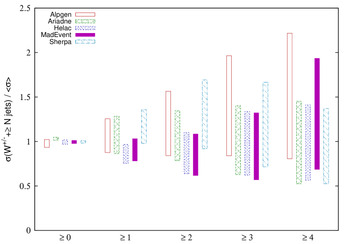
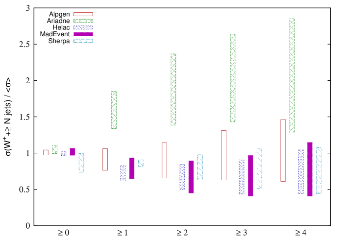
We present here the comparison among inclusive jet rates. These are shown in table 1. For each code, in addition to the default numbers, we present the results of the various individual alternative choices used to assess the systematics uncertainty. In table 2 we show the “additional jet fractions”, namely the rates , once again covering all systematic sets of all codes. Fig. 1, finally, shows graphically the cross-section systematic ranges: for each multiplicity, we normalize the rates to the average of the default values of all the codes.
It should be noted that the scale changes in all codes lead to the largest rate variations. This is reflected in the growing size of the uncertainty with larger multiplicities, a consequence of the higher powers of . A more detailed discussion on the effects of the scale changes can be found in section 6. Furthermore we note that the systematic ranges of all codes have regions of overlap.
| Code | [tot] | [ jet] | [ jet] | [ jet] | [ jet] |
|---|---|---|---|---|---|
| A LPGEN , def | 1933 | 444 | 97.1 | 18.9 | 3.2 |
| ALpt20 | 1988 | 482 | 87.2 | 15.5 | 2.8 |
| ALpt30 | 2000 | 491 | 82.9 | 12.8 | 2.1 |
| ALscL | 2035 | 540 | 135 | 29.7 | 5.5 |
| ALscH | 1860 | 377 | 72.6 | 12.7 | 2.0 |
| A RIADNE , def | 2066 | 477 | 87.3 | 13.9 | 2.0 |
| ARpt20 | 2038 | 459 | 76.6 | 12.8 | 1.9 |
| ARpt30 | 2023 | 446 | 67.9 | 11.3 | 1.7 |
| ARscL | 2087 | 553 | 116 | 21.2 | 3.6 |
| ARscH | 2051 | 419 | 67.8 | 9.5 | 1.3 |
| ARs | 2073 | 372 | 80.6 | 13.2 | 2.0 |
| H ELAC , def | 1960 | 356 | 70.8 | 13.6 | 2.4 |
| HELpt30 | 1993 | 373 | 68.0 | 12.5 | 2.4 |
| HELscL | 2028 | 416 | 95.0 | 20.2 | 3.5 |
| HELscH | 1925 | 324 | 55.1 | 9.4 | 1.4 |
| M AD E VENT , def | 2013 | 381 | 69.2 | 12.6 | 2.8 |
| MEkt20 | 2018 | 375 | 66.7 | 13.3 | 2.7 |
| MEkt30 | 2017 | 361 | 64.8 | 11.1 | 2.0 |
| MEscL | 2013 | 444 | 93.6 | 20.0 | 4.8 |
| MEscH | 1944 | 336 | 53.2 | 8.6 | 1.7 |
| S HERPA , def | 1987 | 494 | 107 | 16.6 | 2.0 |
| SHkt20 | 1968 | 465 | 85.1 | 12.4 | 1.5 |
| SHkt30 | 1982 | 461 | 79.2 | 10.8 | 1.3 |
| SHscL | 1957 | 584 | 146 | 25.2 | 3.4 |
| SHscH | 2008 | 422 | 79.8 | 11.2 | 1.3 |
| Code | / | / | / | / |
|---|---|---|---|---|
| A LPGEN , def | 0.23 | 0.22 | 0.19 | 0.17 |
| ALpt20 | 0.24 | 0.18 | 0.18 | 0.18 |
| ALpt30 | 0.25 | 0.17 | 0.15 | 0.16 |
| ALscL | 0.27 | 0.25 | 0.22 | 0.19 |
| ALscH | 0.20 | 0.19 | 0.17 | 0.16 |
| A RIADNE , def | 0.23 | 0.18 | 0.16 | 0.15 |
| ARpt20 | 0.23 | 0.17 | 0.17 | 0.15 |
| ARpt30 | 0.22 | 0.15 | 0.16 | 0.16 |
| ARscL | 0.26 | 0.21 | 0.18 | 0.17 |
| ARscH | 0.20 | 0.16 | 0.14 | 0.14 |
| ARs | 0.18 | 0.22 | 0.16 | 0.15 |
| H ELAC , def | 0.18 | 0.20 | 0.19 | 0.18 |
| HELpt30 | 0.19 | 0.19 | 0.18 | 0.19 |
| HELscL | 0.21 | 0.23 | 0.21 | 0.17 |
| HELscH | 0.17 | 0.17 | 0.17 | 0.15 |
| M AD E VENT , def | 0.19 | 0.18 | 0.18 | 0.22 |
| MEkt20 | 0.19 | 0.18 | 0.20 | 0.20 |
| MEkt30 | 0.18 | 0.18 | 0.17 | 0.18 |
| MEscL | 0.22 | 0.21 | 0.21 | 0.24 |
| MEscH | 0.17 | 0.16 | 0.16 | 0.20 |
| S HERPA , def | 0.25 | 0.22 | 0.16 | 0.12 |
| SHkt20 | 0.24 | 0.18 | 0.15 | 0.12 |
| SHkt30 | 0.23 | 0.17 | 0.14 | 0.12 |
| SHscL | 0.30 | 0.25 | 0.17 | 0.13 |
| SHscH | 0.21 | 0.19 | 0.14 | 0.12 |
4.2 Kinematical distributions
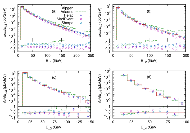
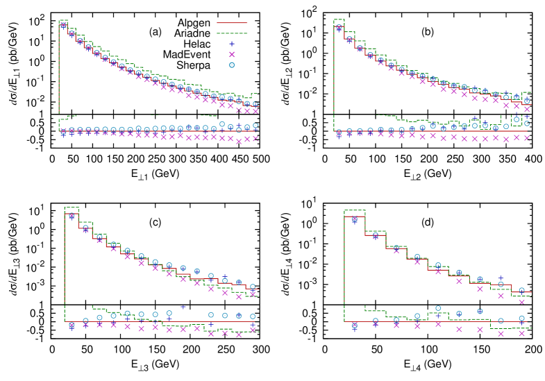
We start by showing in fig. 2 the inclusive spectra of the leading 4 jets. The absolute rate predicted by each code is used, in units of pb/GeV. The relative differences with respect to the A LPGEN results, in this figure and all other figures of this section, are shown in the lower in-sets of each plot, where for the code we plot the quantity , being the values of the A LPGEN curves.
There is generally good agreement between the codes, except for A RIADNE , which has a harder spectra for the leading two jets. There we also find that S HERPA is slightly harder than A LPGEN and H ELAC , while M AD E VENT is slightly softer.
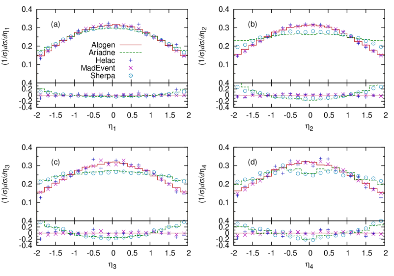
Fig. 3 shows the inclusive spectra of the leading 4 jets, all normalized to unit area. There is a good agreement between the spectra of A LPGEN , H ELAC and M AD E VENT , while A RIADNE and S HERPA spectra appear to be broader, in particular for the sub-leading jets. This broadening is expected for A RIADNE since the gluon emissions there are essentially unordered in rapidity, which means that the Sudakov form factors applied to the matrix-element-generated states include also a resummation absent in the other programs.
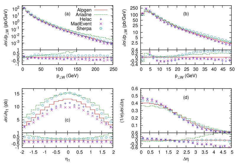
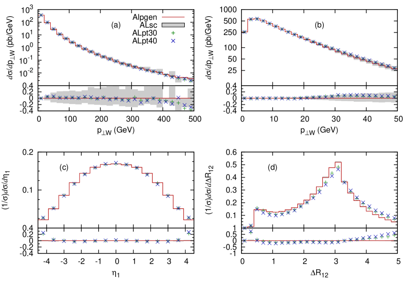
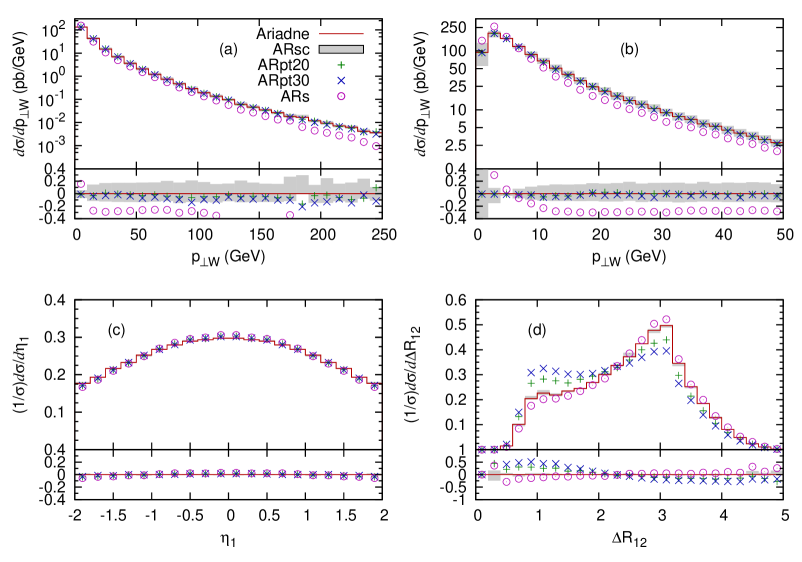
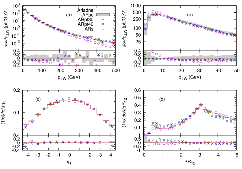
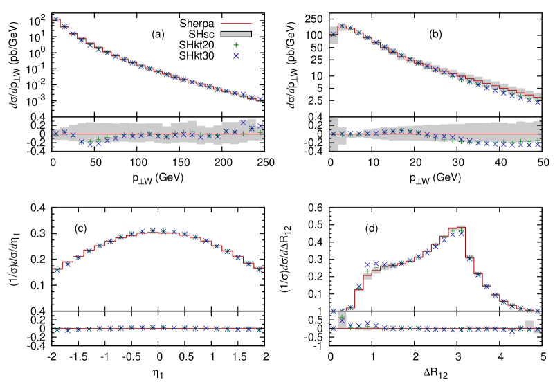
Fig. 4a shows the inclusive distribution of the boson, with absolute normalization in pb/GeV. This distribution reflects in part the behaviour observed for the spectrum of the leading jet, with A RIADNE harder than S HERPA , which, in turn, is slightly harder than A LPGEN , H ELAC and M AD E VENT . The region of low momenta, GeV, is expanded in fig. 4b. Fig. 4c shows the distribution of the leading jet, , when its transverse momentum is larger than 50 GeV. The curves are absolutely normalized, so that it is clear how much rate is predicted by each code to survive this harder jet cut. The separation between the and the leading jet of the event above 30 GeV is shown in fig. 4d, normalized to unit area. Here we find that A RIADNE has a broader correlation, while H ELAC and M AD E VENT are somewhat more narrow than A LPGEN and S HERPA .
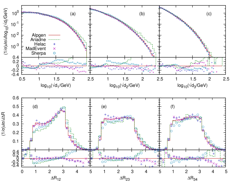
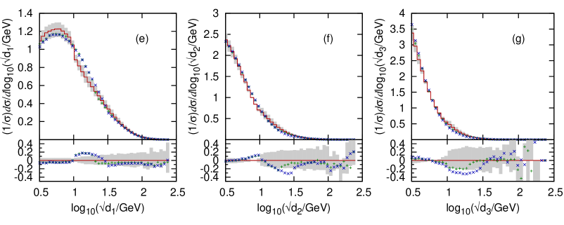
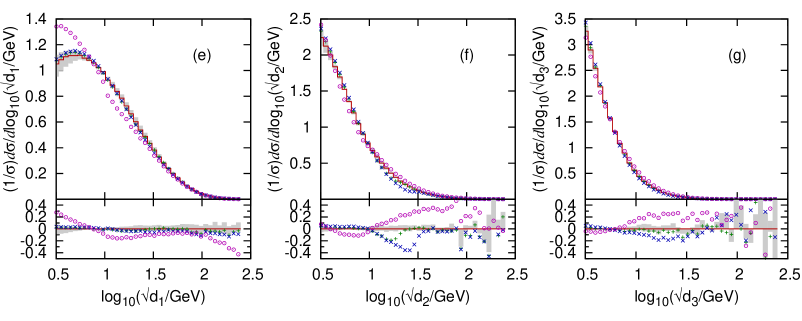
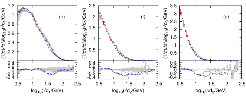
In fig. 5 we show the merging scales as obtained from the -algorithm, where is the scale in an event where jets are clustered into jets. These are parton-level distributions and are especially sensitive to the behaviour of the merging procedure close to the merging/matching scale. Note that in the plots showing the difference the wiggles stem from both the individual codes and from the A LPGEN reference. In section 6 below, the behaviour of the individual codes is treated separately.
Also shown in fig. 5 is the separation in between successive jet pairs ordered in hardness. The is dominated by the transversal-plane back-to-back peak at , while for larger in all cases the behaviour is more dictated by the correlations in pseudo-rapidity. For these larger values we find a weaker correlation in A RIADNE and S HERPA , which can be expected from their broader rapidity distributions in fig. 3.
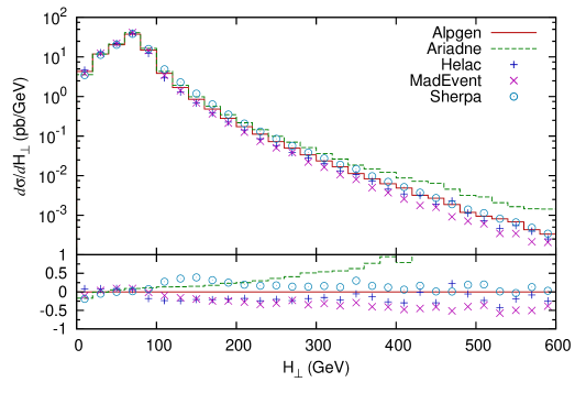
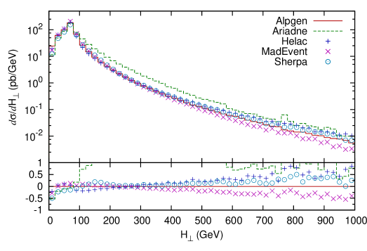
Finally, in fig. 6 we show , the scalar sum of the transverse momenta of the charged lepton, the neutrino and the jets. This is a variable in which one often does experimental cuts in searches for new phenomena and is not expected to be very sensitive to the particulars in the merging schemes. The results show good agreement below 100 GeV, but at higher values, as expected from the differences in the hardness of the jet and spectra, A RIADNE has a harder spectra than S HERPA and A LPGEN , while M AD E VENT and H ELAC has a slightly softer spectra.
5 LHC Studies
5.1 Event rates
The tables (table 3 and 4) and figure (fig. 7) of this section parallel those shown earlier for the Tevatron. The largest rate variations is, similarly to the Tevatron rates, determined by the scale changes (described in more detail in section 6). The main feature of the LHC results is the significantly larger rates predicted by A RIADNE (see also the discussion of its systematics, section 6.2), which are outside the systematics ranges of the other codes. Aside from this and the fact that S HERPA gives a smaller total cross section (see also the last part of the discussion of the S HERPA systematics in section 6.5), the comparison among the other codes shows an excellent consistency, with a pattern of the details similar to what seen for the Tevatron.
| Code | [tot] | [ jet] | [ jet] | [ jet] | [ jet] |
|---|---|---|---|---|---|
| A LPGEN , def | 10170 | 2100 | 590 | 171 | 50 |
| ALpt30 | 10290 | 2200 | 555 | 155 | 46 |
| ALpt40 | 10280 | 2190 | 513 | 136 | 41 |
| ALscL | 10590 | 2520 | 790 | 252 | 79 |
| ALscH | 9870 | 1810 | 455 | 121 | 33 |
| A RIADNE , def | 10890 | 3840 | 1330 | 384 | 101 |
| ARpt30 | 10340 | 3400 | 1124 | 327 | 88 |
| ARpt40 | 10090 | 3180 | 958 | 292 | 83 |
| ARscL | 11250 | 4390 | 1635 | 507 | 154 |
| ARscH | 10620 | 3380 | 1071 | 275 | 69 |
| ARs | 11200 | 3440 | 1398 | 438 | 130 |
| H ELAC , def | 10050 | 1680 | 442 | 118 | 36 |
| HELpt40 | 10150 | 1760 | 412 | 116 | 37 |
| HELscL | 10340 | 1980 | 585 | 174 | 57 |
| HELscH | 9820 | 1470 | 347 | 84 | 24 |
| M AD E VENT , def | 10830 | 2120 | 519 | 137 | 42 |
| MEkt30 | 10080 | 1750 | 402 | 111 | 37 |
| MEkt40 | 9840 | 1540 | 311 | 78.6 | 22 |
| MEscL | 10130 | 2220 | 618 | 186 | 62 |
| MEscH | 10300 | 1760 | 384 | 91.8 | 27 |
| S HERPA , def | 8800 | 2130 | 574 | 151 | 41 |
| SHkt30 | 8970 | 2020 | 481 | 120 | 32 |
| SHkt40 | 9200 | 1940 | 436 | 98.5 | 24 |
| SHscL | 7480 | 2150 | 675 | 205 | 58 |
| SHscH | 10110 | 2080 | 489 | 118 | 30 |
| Code | / | / | / | / |
|---|---|---|---|---|
| A LPGEN , def | 0.21 | 0.28 | 0.29 | 0.29 |
| ALpt30 | 0.21 | 0.25 | 0.28 | 0.30 |
| ALpt40 | 0.21 | 0.23 | 0.27 | 0.30 |
| ALscL | 0.24 | 0.31 | 0.32 | 0.31 |
| ALscH | 0.18 | 0.25 | 0.27 | 0.27 |
| A RIADNE , def | 0.35 | 0.35 | 0.29 | 0.26 |
| ARpt30 | 0.33 | 0.33 | 0.29 | 0.27 |
| ARpt40 | 0.32 | 0.30 | 0.30 | 0.28 |
| ARscL | 0.39 | 0.37 | 0.31 | 0.30 |
| ARscH | 0.32 | 0.32 | 0.26 | 0.24 |
| ARs | 0.31 | 0.41 | 0.31 | 0.30 |
| H ELAC , def | 0.17 | 0.26 | 0.27 | 0.31 |
| HELpt40 | 0.17 | 0.23 | 0.28 | 0.32 |
| HELscL | 0.19 | 0.30 | 0.30 | 0.33 |
| HELscH | 0.15 | 0.24 | 0.24 | 0.29 |
| M AD E VENT , def | 0.20 | 0.24 | 0.26 | 0.31 |
| MEkt30 | 0.17 | 0.23 | 0.28 | 0.33 |
| MEkt40 | 0.16 | 0.20 | 0.25 | 0.28 |
| MEscL | 0.22 | 0.27 | 0.30 | 0.34 |
| MEscH | 0.17 | 0.22 | 0.24 | 0.29 |
| S HERPA , def | 0.24 | 0.27 | 0.26 | 0.27 |
| SHkt30 | 0.23 | 0.24 | 0.25 | 0.27 |
| SHkt40 | 0.21 | 0.22 | 0.23 | 0.24 |
| SHscL | 0.29 | 0.31 | 0.30 | 0.28 |
| SHscH | 0.21 | 0.24 | 0.24 | 0.25 |
5.2 Kinematical distributions
Following the same sequence of the Tevatron study, we start by showing in fig. 8 the inclusive spectra of the leading 4 jets. The absolute rate predicted by each code is used, in units of pb/GeV.
Except for A RIADNE , we find good agreement among the codes, with A RIADNE having significantly harder leading jets, while for sub-leading jets the increased rates noted in fig. 7 mainly come from lower . Among the other codes, H ELAC and S HERPA have consistently somewhat harder jets than A LPGEN , while M AD E VENT is a bit softer, but these differences are not as pronounced.
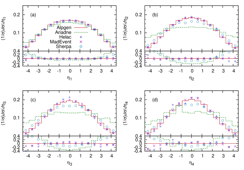

For the pseudo-rapidity spectra of the jets in fig. 9 it is clear that A RIADNE has a much broader distribution in all cases. Also S HERPA has broader distributions, although not as pronounced, while the other codes are very consistent.
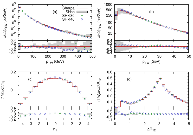
The distribution of bosons in fig. 10 follows the trend of the leading-jet spectra. The differences observed in the region below 10 GeV are not due to the choice of merging approach, but are entirely driven by the choice of shower algorithm. Notice for example the similarity of the H ELAC and M AD E VENT spectra, and their peaking at lower pt than the H ERWIG spectrum built into the A LPGEN curve, a result well known from the comparison of the standard P YTHIA and H ERWIG generators. Increasing the transverse momentum of the leading jet in fig. 10a does not change the conclusions much for its pseudo-rapidity distribution. Also the rapidity correlation between the leading jet and the follows the trend found for the Tevatron, but the differences are larger, with a much weaker correlation for A RIADNE . Also S HERPA shows a somewhat weaker correlation, while H ELAC is somewhat stronger than A LPGEN and M AD E VENT .
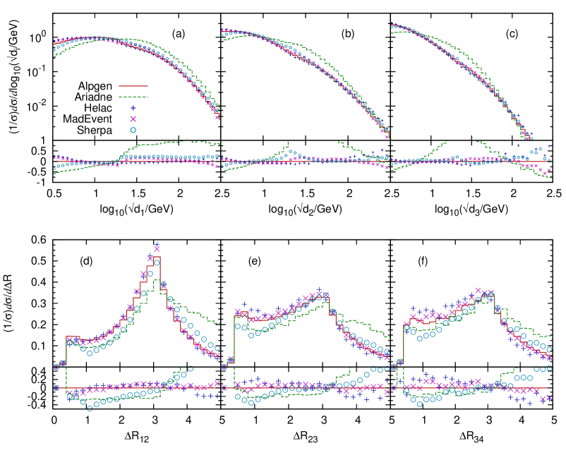
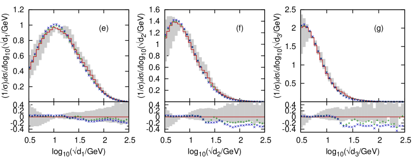
For the distribution in clustering scale in fig. 11, we find again that A RIADNE is by far the hardest. The results given by the other codes are comparable, with the only exception that for the distribution, S HERPA gives a somewhat harder prediction compared to the ones made by the MLM-based approaches.
The distributions, in fig. 11, show at large separation a behaviour consistent with the broad rapidity distributions found for S HERPA , and in particular for A RIADNE , in fig. 9. This increase at large is then compensated by a depletion with respect to the other codes at small separation.
The scalar transverse momentum sum in fig. 12 shows significantly larger deviations as compared to the results for the Tevatron. A RIADNE has a much harder spectra than the other codes, while S HERPA and H ELAC are slightly harder than A LPGEN and M AD E VENT is significantly softer. As in the Tevatron case, it is a direct reflection of the differences in the hardness of the jet and spectra, although the increased phase space for jet production at the LHC makes the contribution less important at high values.
6 Systematic studies
In this section we present the systematic studies of each of the codes separately for both the Tevatron and the LHC, followed by some general comments on differences and similarities between the codes.
In all cases we have chosen a subset of the plots shown in the previous sections: the transverse momentum of the , the pseudo-rapidity of the leading jet, the separation between the leading and the sub-leading jet, and the logarithmic spectra. As before, all spectra aside from are normalized to unit integral over the displayed range. The variations of the inclusive jet cross sections has already been shown in table 1-4 and figs. 1 and 7.
To estimate what systematic error can be expected from each code, the effects of varying the merging scale and changing the scale used in the determination of the strong coupling is studied (the details for each code is described in section 3). The merging scale variations are introduced according to the definition in each algorithms and should lead to small changes in the results, although the nonleading terms from the matrix elements always lead to some residual dependence on the merging scale. In the various algorithms different choices have been made regarding how to estimate the uncertainty from -scale variations and this leads to slightly different physical consequences.
In the case of A LPGEN and H ELAC , the scale changes are only implemented in the strong coupling calculated in the matrix element reweighting, but the scale in the shower remains unchanged. This leads to variations of the result that are proportional to the relevant power of used in the matrix element, which means that the spectra contains small deviations below the merging scale and that the deviations grow substantially above the merging scale.
In A RIADNE , M AD E VENT and S HERPA both the scale in the -reweighting and the scale in the of the shower is changed. In addition to this the scale used in the evaluation of the parton densities is also changed in S HERPA (this is discussed further in section 6.5). Including the scale variations in in the shower changes the fraction of rejected events or the Sudakov form factors (depending on which algorithm is used), which modifies the cross section in the opposite direction compared to the scale changes in the matrix element reweighting. This leads to smaller deviations in the results above the merging scale and it is also possible to get significant deviations in the opposite direction below the merging scale, which is mainly visible in the spectra.

6.1 A LPGEN systematics
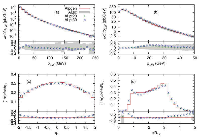
The A LPGEN distributions for the Tevatron are shown in fig. 13. The pattern of variations is consistent with the expectations. In the case of the spectra, which are plotted in absolute scales, the larger variations are due to the change of scale, with the lower scale leading to a harder spectrum. The effect is consistent with the scale variation of , which dominates the scale variation of the rate once is larger than the Sudakov region. The change of matching scales only leads to a minor change in the region GeV, confirming the stability of the merging prescription.
In the case of the rapidity spectrum, we notice that the scale change leaves the shape of the distribution unaltered, while small changes appear at the edges of the range. The distributions show agreement among the various options when GeV. This is due to the fact that the region GeV is dominated by the initial-state evolution of an parton event, and both the matching and scale sensitivities are reduced. Notice that in the A LPGEN prescription the scale for the shower evolution is kept fixed when the renormalization scale of the matrix elements is changed, as a way of exploring the impact of a possible mismatch between the two.
For the jet transverse energies are themselves typically above , and the sensitivity to matching thresholds smaller than is reduced, since if the event matched at , it will also match below that. Here the main source of systematics is therefore the scale variation, associated to the hard matrix element calculation for the jet multiplicity. The region is the transition region between the dominance of the shower and of the matrix element description of hard radiation. The structure observed in the distributions in this region reflects the fact that shower and matrix element emit radiation with a slightly different probability. The selection of a matching threshold, which leads to effects at the level of and is therefore consistent with a LL accuracy and can be used to tune to data.
For the LHC, the A LPGEN systematics is shown in fig. 14. The comparison of the various parameter choices is similar to what we encountered at the Tevatron, with variations in the range of for the matching-scale systematics, and up to 40% for the scale systematics. The pattern of the glitches in the spectra for the different matching thresholds is also consistent with the explanation provided in the case of the Tevatron.
6.2 A RIADNE systematics

The A RIADNE systematics for the Tevatron is shown in fig. 15. Since the dipole cascade by itself already includes a matrix-element correction for the first emission, we see no dependence on the merging scale in the , and distributions, which are mainly sensitive to leading order corrections. For the other distributions, we become sensitive to higher-order corrections, and here the pure dipole cascade underestimates the matrix element and also tends to make the leading jets less back-to-back in azimuth. The first effect is expected for all parton showers, but is somewhat enhanced in A RIADNE due to the missing initial-state splitting, and is mostly visible in the distribution just below the merging scale. The second effect is clearly visible in the distribution, which is dominated by low jets.
The changing of the soft suppression parameter in ARs has the effect of reducing the available phase space of gluon radiation, especially for large and in the beam directions, an effect, which is mostly visible for the hardest emission and in the distribution. As for A LPGEN , and also for the other codes, the change in scale mainly affects the hardness of the jets, but not the and the distribution.
For the LHC, the A RIADNE systematics is shown in fig. 16. Qualitatively we find the same effects as in the Tevatron case. In particular we note the strong dependence on the soft suppression parameters in ARs, and it is clear that these have to be adjusted to fit Tevatron (and HERA) data before any predictions for the LHC can be made. It should be noted, however, that while eg. the high tail in fig. 16a for ARs is shifted down to be comparable to the other codes (cf. fig. 10a), the medium values are less affected and here the differences compared to the other codes can be expected to remain after a retuning.
This difference is mainly due to the fact that the dipole cascade in A RIADNE , contrary to the other parton showers, is not based on standard DGLAP evolution, but also allows for evolution, which is unordered in transverse momentum à la BFKL555The dipole emission of gluons in A RIADNE are ordered in transverse momentum, but not in rapidity. Translated into a conventional initial-state evolution, this corresponds to emissions ordered in rapidity but unordered in transverse momentum.. This means that in A RIADNE there is also a resummation of logs of besides the standard resummation. This should not be a large effect at the Tevatron, and the differences there can be tuned away by changing the soft suppression parameters in A RIADNE . However, at the LHC we have quite small -values, , which allow for a much increased phase space for jets as compared to what is allowed by standard DGLAP evolution. As a result one obtains larger inclusive jet rates as documented in table 3. The same effect is found in DIS at HERA, where is even smaller as are the typical scales, . And here, all DGLAP-based parton showers fail to reproduce final-state properties, especially forward jet rates, while A RIADNE does a fairly good job.
It would be interesting to compare the merging schemes presented here also to HERA data to see if the DGLAP based shower would better reproduce data when merged with higher-order matrix elements. This would also put the extrapolations to the LHC on safer grounds. However, so far there exists one preliminary such study for the A RIADNE case only[53].
6.3 H ELAC systematics


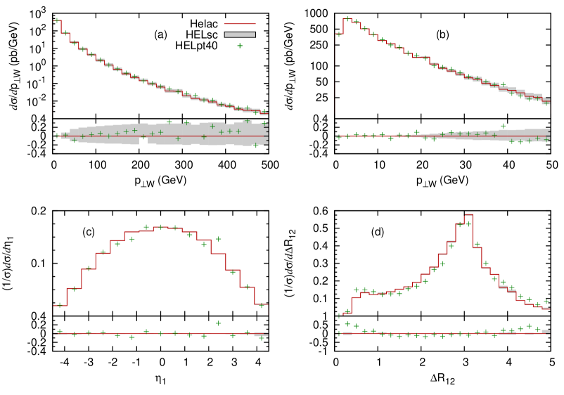
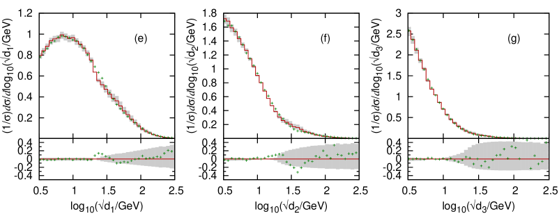
The Tevatron H ELAC distributions are shown in fig. 17. Since H ELAC results presented in this study are based on the MLM matching prescription, we expect the H ELAC systematics to follow at least qualitatively the A LPGEN ones and this is indeed the case. On the other hand the use by H ELAC of P YTHIA , for parton showering as well as for hadronization, leads to differences compared to the A LPGEN results, where H ERWIG is used. For the absolute rates, especially in the multi-jet regime, H ELAC seems to be closer to M AD E VENT that also uses P YTHIA .
For the LHC, the H ELAC systematics are shown in fig. 18. The systematics follows a similar pattern compared to that already discussed for the Tevatron case, with the expected increase of up to 40% from scale variations, due to the higher collision energy.
6.4 M AD E VENT systematics


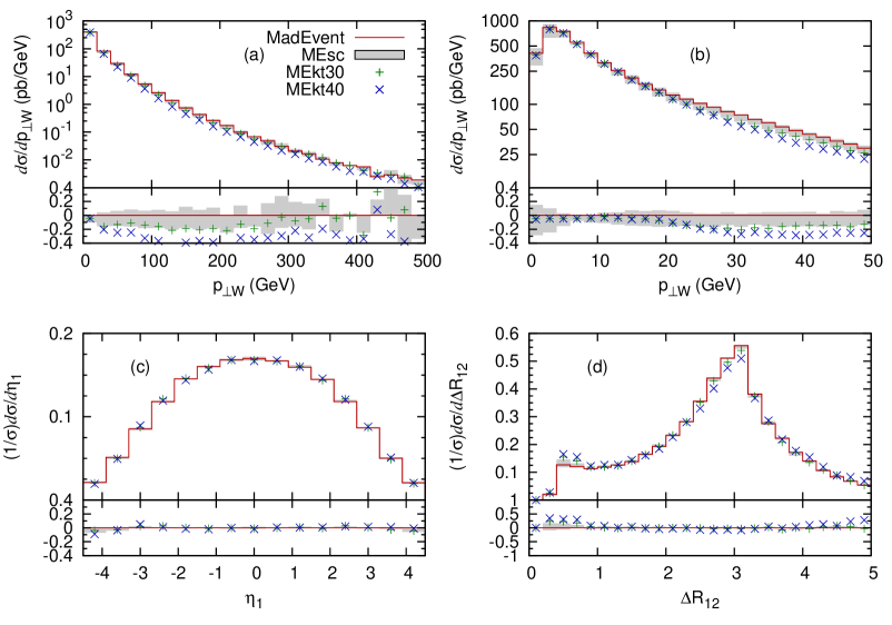

The M AD E VENT distributions for the Tevatron are shown in fig. 19. Also here, the variations are consistent with the expectations. For the spectrum, the dominant variations are due to the change of scale for , with the lower scale leading to a harder spectrum. Below the -cutoff, where the distribution is determined by the parton shower only, the lower scale gives the lower differential cross section.
At Tevatron energies, both the spectrum and the spectra are relatively stable with respect to variations of the matching scale. For the spectra, the variation in matching scale gives a dip in the region , but is reduced for larger . The rapidity and jet-distance spectra show a remarkable stability under both renormalization-scale changes and variations in the cutoff scale.
For the LHC, the systematics of the M AD E VENT implementation are shown in fig. 20. The variations in renormalization scale give a very similar effect as for the Tevatron, with variations up to on the and spectra. For variations in the matching scale , however, the pattern is slightly different. This can be most easily understood from looking at the spectra, since, as in the Sherpa case, the cutoff scale is defined to be just the , so the transition between the parton-shower and matrix-element regions is very sharp. It is clear from these distributions that the default parton shower of P YTHIA does not reproduce the shape of the matrix elements at LHC energies even for relatively small , but falls off more sharply. There is therefore a dip in all the distributions around , which gets more pronounced for the higher multiplicity distributions, and hence gives lower overall jet rates. The distributions, as well as the distributions, are composed of all the different jet-multiplicity samples, which gives systematically reduced hardness of the differential cross sections for increased cutoff scales. These effects are clearly visible also in S HERPA , which uses a P YTHIA -like parton shower and as merging scale.
6.5 S HERPA systematics
The systematics of the CKKW algorithm as implemented in S HERPA is presented in fig. 21 for the Tevatron case. The effect of varying the scales in the PDF and strong coupling evaluations by a factor of is that for the lower (higher) scale choice, the -boson’s spectrum becomes harder (softer). For this kind of observables the uncertainties given by scale variations dominate the ones emerging through variations of the internal separation cut. This is mainly due to a reduced (enhanced) suppression of hard-jet radiation through the rejection weights. The differential jet rates, , shown in fig. 21e–g, have a more pronounced sensitivity on the choice of the merging scale, leading to variations at the level. In the CKKW approach this dependence can be understood since the -measure intrinsically serves as the discriminator to separate the matrix-element and parton-shower regimes. Hence, the largest deviations from the default typically appear at . However, the results are remarkably smooth, which leads to the conclusion that the cancellation of the dominant logarithmic dependence on the merging cut is well achieved. Moreover, considering the pseudo-rapidity of the leading jet and the cone separation of the two hardest jets, these distributions show a very stable behaviour under the studied variations, since they are indirectly influenced by the cut scale only. The somewhat more pronounced deviation at low is connected to phase-space regions of jets becoming close together, which is affected by the choice of the merging scale and therefore by its variation. Taken together, S HERPA produces consistent results with relative differences of the order of or less than at Tevatron energies.
The S HERPA studies of systematics for the LHC are displayed in fig. 22. Compared to the Tevatron case, a similar pattern of variations is recognized. The spectra of the boson show deviations under cut and scale variations that remain on the same order of magnitude. However, a noticeable difference is an enhancement of uncertainties in the predictions for low . This phase-space region is clearly dominated by the parton shower evolution, which in the S HERPA treatment of estimating uncertainties undergoes scale variations in the same manner as the matrix-element part. Therefore, the estimated deviations from the default given for low are very reasonable and reflect intrinsic uncertainties underlying the parton showering. For the LHC case, the effect is larger, since the evolution is dictated by steeply rising parton densities at -values that are lower compared to the Tevatron scenario. The pseudo-rapidity of the leading jet and the cone separation of the two hardest jets show again a stable behaviour under the applied variations, the only slight exception is the regions of high where, using a high -cut, the deviations are at the level. The effect of varying the scales in the parton distributions and strong couplings now dominates the uncertainties in the differential jet rates, , which are presented in fig. 22e–g. This time, owing to the larger phase space, for the low scale choice, , the spectra become up to harder, whereas, for the high scale choice, the spectra are up to softer. The variation of the internal merging scale does not induce jumps around the cut region, however it has to be noted that for higher choices, e.g. GeV, there is a tendency to predict softer distributions in the tails compared to the default. To summarize, the extrapolation from Tevatron to LHC energies does not yield significant changes in the predictions of uncertainties under merging-cut and scale variations; for the LHC scenario, they have to be estimated slightly larger, ranging up to . The results are again consistent and exhibit a well controlled behaviour when applying the CKKW approach implemented in S HERPA at LHC energies.
Giving a conservative, more reliable estimate, in S HERPA the strategy of varying the scales in the strong coupling together with the scales in the parton densities has been chosen to assess its systematics. So, to better estimate the impact of the additional scale variation in the parton density functions, renormalization-scale variations on its own have been studied as well. Their results show smaller deviations wrt. the default in the observables of this study with the interpretation of potentially underestimating the systematics of the merging approach. Also, then the total cross sections vary less and become pb and pb for the low- and high-scale choice, respectively. Note that, owing to the missing simultaneous factorization-scale variation, their order is now reversed compared to SHscL and SHscH, whose values are given in table 3. Moreover, by referring to table 4 the cross-section ratios for e.g. / now read and for the low- and high-scale choice, respectively. This once more emphasizes that the approach’s uncertainty may be underestimated when relying on -scale variations only. From table 3 it also can be noted that the total inclusive cross section given by the full high-scale prediction SHscH is – unlike S HERPA ’s default – close to the A LPGEN default. In contrast to the MLM-based approaches, which prefer the factorization scale in the matrix-element evaluation set through the transverse mass of the weak boson, the S HERPA approach makes the choice of employing the merging scale instead. This has been motivated in [9] and further discussed in [3]. Eventually, it is a good result that compatibility is achieved under this additional PDF-scale variation for the total inclusive cross sections, however it also clearly stresses that there is a non-negligible residual dependence on the choice of the factorization scale in the merging approaches.
6.6 Summary of the systematics studies
Starting with the spectra, we find a trivial % effect of the scale changes, with the lower scale leading to a harder spectrum. In the case of A LPGEN and H ELAC , this only affects the spectrum above the matching scale, while for A RIADNE , M AD E VENT and S HERPA there is also an effect below, as there the scale change is also implemented in the parton shower. For all the codes the change in merging/matching scale gives effects smaller than or of the order of the change in scale. For A RIADNE , the change in the soft suppression parameter (ARs) gives a softer spectrum, which is expected as it directly reduces the phase space for emitted gluons.
In the and distributions the effects of changing the scale in are negligible. In all cases, changing the merging/matching scale also has negligible effects on the rapidity spectrum, while the tends to become more peaked at small values for larger merging/matching scales, and also slightly less peaked at . This effect is largest for A RIADNE while almost absent for H ELAC .
Finally for the distributions we clearly see wiggles of varying sizes introduced by changing the merging scales.
7 Conclusions
This document summarizes our comparisons of five independent approaches to the problem of merging matrix elements and parton showers. The codes under study, A LPGEN , A RIADNE , H ELAC , M AD E VENT and S HERPA , differ in which matrix-element generator is used, which merging scheme (CKKW or MLM) is used and the details in the implementation of these schemes, as well as in which parton shower is used.
We find that, while the three approaches (CKKW, L, and MLM) aim at a simulation based on the same idea, namely describing jet production and evolution by matrix elements and the parton shower, respectively, the corresponding algorithms are quite different. The main differences can be found in the way in which the combination of Sudakov reweighting of the matrix elements interacts with the vetoing of unwanted jet production inside the parton shower. This makes it very hard to compare those approaches analytically and to formalise the respective level of their logarithmic dependence. In addition, the different showering schemes used by the different methods blur the picture further. For instance virtuality ordering with explicit angular vetoes is used in S HERPA as well as in the H ELAC and M AD E VENT approach employ P YTHIA to do the showering, ordering is the characteristic feature of A RIADNE , and, through its usage of H ERWIG it is angular ordering that enters into the A LPGEN merging approach. However, although the formal level of agreement between the codes is not worked out in this publication and remains unclear, the results presented in this publication show a reasonably good agreement. This proves that the variety of methods for merging matrix elements and parton showers can be employed with some confidence in vector boson plus jet production.
The comparison also points to differences, in absolute rates as well as in the shape of individual distributions, which underscore the existence of an underlying systematic uncertainty. Most of these differences are at a level that can be expected from merging tree-level matrix elements with leading-log parton showers, in the sense that they are smaller than, or of the order of, differences found by making a standard change of scale in . In most cases the differences within each code are as large as the differences between the codes. And as the systematics at the Tevatron is similar to that at the LHC, it is conceivable that all the codes can be tuned to Tevatron data to give consistent predictions for the LHC. To carry out such tunings, we look forward to the publication by CDF and DØ of the measured cross sections for distributions such as those considered in this paper, fully corrected for all detector effects.
Acknowledgments
Work supported in part by the Marie Curie research training networks “MCnet” (contract number MRTN-CT-2006-035606) and “HEPTOOLS” (MRTN-CT-2006-035505).
C.G. Papadopoulos and M. Worek would like to acknowledge support from the ToK project ALGOTOOLS, “Algorithms and tools for multi-particle production and higher order corrections at high energy colliders”, (contract number MTKD-CT-2004-014319).
M. Worek and S. Schumann want to thank DAAD for support through the Dresden–Crakow exchange programme.
J. Winter acknowledges financial support by the Marie Curie Fellowship program for Early Stage Research Training and thanks the CERN Theory Division for the great hospitality during the funding period.
J. Alwall acknowledges financial support by the Swedish Research Council.
References
- [1] S. Mrenna and P. Richardson JHEP 05 (2004) 040 [hep-ph/0312274].
- [2] S. Höche et. al. [hep-ph/0602031].
- [3] F. Krauss, A. Schälicke, S. Schumann and G. Soff Phys. Rev. D70 (2004) 114009 [hep-ph/0409106].
- [4] F. Krauss, A. Schälicke, S. Schumann and G. Soff Phys. Rev. D72 (2005) 054017 [hep-ph/0503280].
- [5] T. Gleisberg, F. Krauss, A. Schälicke, S. Schumann and J. Winter Phys. Rev. D72 (2005) 034028 [hep-ph/0504032].
- [6] N. Lavesson and L. Lönnblad JHEP 07 (2005) 054 [hep-ph/0503293].
- [7] M. L. Mangano, M. Moretti, F. Piccinini and M. Treccani JHEP 01 (2007) 013 [hep-ph/0611129].
- [8] S. Catani, F. Krauss, R. Kuhn and B. R. Webber JHEP 0111 (2001) 063–084 [hep-ph/0109231].
- [9] F. Krauss JHEP 0208 (2002) 015–031 [hep-ph/0205283].
- [10] T. Gleisberg, S. Höche, F. Krauss, A. Schälicke, S. Schumann and J. Winter JHEP 0402 (2004) 056 [hep-ph/0311263].
- [11] A. Schälicke and F. Krauss JHEP 07 (2005) 018 [hep-ph/0503281].
- [12] S. Catani, Y. L. Dokshitser, M. Olsson, G. Turnock and B. R. Webber Phys. Lett. B 269 (1991) 432.
- [13] S. Catani, Y. L. Dokshitser and B. R. Webber Phys. Lett. B 285 (1992) 291.
- [14] S. Catani, Y. L. Dokshitser and B. R. Webber Nucl. Phys. B 406 (1993) 187.
- [15] G. C. Blazey et. al. [hep-ex/0005012].
- [16] L. Lönnblad Comput. Phys. Commun. 71 (1992) 15–31.
- [17] G. Gustafson and U. Pettersson Nucl. Phys. B306 (1988) 746.
- [18] G. Gustafson Phys. Lett. B175 (1986) 453.
- [19] B. Andersson, G. Gustafson and L. Lönnblad Nucl. Phys. B339 (1990) 393–406.
- [20] B. Andersson, G. Gustafson, L. Lönnblad and U. Pettersson Z. Phys. C43 (1989) 625.
- [21] L. Lönnblad Nucl. Phys. B458 (1996) 215–230 [hep-ph/9508261].
- [22] H1 Collaboration, A. Aktas et. al. Eur. Phys. J. C46 (2006) 27–42 [hep-ex/0508055].
- [23] L. Lönnblad Z. Phys. C65 (1995) 285–292.
- [24] L. Lönnblad JHEP 05 (2002) 046 [hep-ph/0112284].
- [25] G. Corcella et. al. JHEP 01 (2001) 010 [hep-ph/0011363].
- [26] T. Sjöstrand et. al. Comput. Phys. Commun. 135 (2001) 238–259 [hep-ph/0010017].
- [27] T. Sjöstrand, L. Lönnblad, S. Mrenna and P. Skands [hep-ph/0308153].
- [28] F. Caravaglios, M. L. Mangano, M. Moretti and R. Pittau Nucl. Phys. B539 (1999) 215–232 [hep-ph/9807570].
- [29] M. L. Mangano, M. Moretti and R. Pittau Nucl. Phys. B632 (2002) 343–362 [hep-ph/0108069].
- [30] M. L. Mangano, M. Moretti, F. Piccinini, R. Pittau and A. D. Polosa JHEP 07 (2003) 001 [hep-ph/0206293].
- [31] T. Stelzer and W. F. Long Comput. Phys. Commun. 81 (1994) 357–371 [hep-ph/9401258].
- [32] F. Maltoni and T. Stelzer JHEP 02 (2003) 027 [hep-ph/0208156].
- [33] J. Alwall et. al. arXiv:0706.2334 [hep-ph].
- [34] T. Sjöstrand, S. Mrenna and P. Skands JHEP 05 (2006) 026 [hep-ph/0603175].
- [35] A. Kanaki and C. G. Papadopoulos Comput. Phys. Commun. 132 (2000) 306–315 [hep-ph/0002082].
- [36] C. G. Papadopoulos and M. Worek Eur. Phys. J. C50 (2007) 843–856 [hep-ph/0512150].
- [37] F. Gianotti et. al. Eur. Phys. J. C39 (2005) 293–333 [hep-ph/0204087].
- [38] T. Gleisberg, F. Krauss, C. G. Papadopoulos, A. Schälicke and S. Schumann Eur. Phys. J. C34 (2004) 173–180 [hep-ph/0311273].
- [39] J. Alwall et. al. Comput. Phys. Commun. 176 (2007) 300–304 [hep-ph/0609017].
- [40] CDF Collaboration, F. Abe et. al. Phys. Rev. Lett. 70 (1993) 4042–4046.
- [41] CDF Collaboration, F. Abe et. al. Phys. Rev. Lett. 79 (1997) 4760–4765 [hep-ex/9709016].
- [42] CDF Collaboration, A. A. Affolder et. al. Phys. Rev. D63 (2001) 072003.
- [43] D0 Collaboration, S. Abachi et. al. Phys. Rev. Lett. 75 (1995) 3226–3231.
- [44] CDF Collaboration, A. Messina arXiv:0708.1380 [hep-ex].
- [45] D0 Collaboration, V. M. Abazov et. al. hep-ex/0608052.
- [46] CDF Collaboration. http://www-cdf.fnal.gov/physics/new/qcd/zjets_07/public.pdf, 2007.
- [47] M. H. Seymour. http://hepwww.rl.ac.uk/theory/seymour/ktclus/.
- [48] N. Brook, R. G. Waugh, T. Carli, R. Mohr and M. Sutton. Prepared for Workshop on Future Physics at HERA (Preceded by meetings 25-26 Sep 1995 and 7-9 Feb 1996 at DESY), Hamburg, Germany, 30-31 May 1996.
- [49] C. G. Papadopoulos Comput. Phys. Commun. 137 (2001) 247–254 [hep-ph/0007335].
- [50] F. Krauss, R. Kuhn and G. Soff JHEP 0111 (2002) 044–156 [arXiv:hep-ph/0109036].
- [51] R. Kuhn, F. Krauss, B. Ivanyi and G. Soff Comput. Phys. Commun. 134 (2001) 223–266 [hep-ph/0004270].
- [52] F. Krauss, A. Schälicke and G. Soff Comput. Phys. Commun. 174 (2006) 876–902 [hep-ph/0503087].
- [53] C. Åberg, “Correcting the colour dipole cascade with fixed order matrix elements in deep inelastic scattering.” Diploma thesis, Lund preprint LU-TP 04-25.