LHC EFT WG Report: Experimental Measurements and Observables
Abstract
The LHC effective field theory working group gathers members of the LHC experiments and the theory community to provide a framework for the interpretation of LHC data in the context of EFT. In this note we discuss experimental observables and corresponding measurements in analysis of the Higgs, top, and electroweak data at the LHC. We review the relationship between operators and measurements relevant for the interpretation of experimental data in the context of a global SMEFT analysis. One of the goals of ongoing effort is bridging the gap between theory and experimental communities working on EFT, and in particular concerning optimised analyses. This note serves as a guide to experimental measurements and observables leading to EFT fits and establishes good practice, but does not present authoritative guidelines how those measurements should be performed.
CERN-LPCC-2022-05
0.1 Introduction
The LHC effective field theory working group (LHC EFT WG) [1] gathers members of the LHC experiments and the theory community to provide a framework for the interpretation of LHC data in the context of effective field theories (EFTs). The LHC EFT WG studies the physics requirements needed to facilitate an interpretation commensurate with the available measurements performed in a wide range of different processes with Higgs bosons, top quarks, and electroweak bosons. It provides recommendations for the use of EFT by the experiments to interpret their data, and a forum for theoretical discussions of EFT issues. This includes recommendations on the theory setup as well as Monte Carlo simulation and other tools needed for EFT analyses. It focuses on recommendations, developments, and combinations that require coordination between the existing WGs (Higgs, Top, Electroweak), in order to allow global EFT analyses inside and outside experimental collaborations. The following six areas of activity have been identified:
-
1.
EFT Formalism;
-
2.
Predictions and Tools;
-
3.
Experimental Measurements and Observables;
-
4.
Fits and Related Systematics;
-
5.
Benchmark Scenarios from UV Models;
-
6.
Flavour.
This note is focussed on the topics from Area 3 devoted to experimental measurements and observables. This activity area covers how observables relate to operators, which measurements are important for a given operator or set of operators, differential/fiducial measurements vs. dedicated ones, identification of optimal observables, machine learning, re-interpretation vs. static, presentation of results: covariance, multi-D likelihood, etc., compatibility with global fits (i.e. assumptions used in deriving measurement and reporting results).
The goal is to study observable, channel, process sensitivities and complementarities:
-
•
Experimental targets: survey of the sensitive channels and corresponding operators;
-
•
Differential distributions, optimal observables, including machine learning, and dedicated EFT measurements, spin density matrices, EFT-optimized fiducial regions, amplitude analyses, angular distributions (e.g. for ), pseudo observables…
-
•
Agreement across experiments (for fiducial regions in particular);
-
•
What observables are most sensitive to new physics? Exploit energy growing effects, non-interferences, and other theoretical knowledge;
-
•
Expected uncertainties: systematics or statistics dominated.
The goal is also to study analysis strategies and experimental outputs, also with a view at legacy measurements and their possible reinterpretation:
-
•
Dedicated EFT extractions by collaborations;
-
•
Differential measurements and the best choice of observables for re-interpretation;
-
•
Presentation of measurements: cross sections, correlations/covariance, multi-D likelihood…
-
•
Experimental systematics related to EFT (e.g. accounting for detector effects);
-
•
Detector effects: unfolding, forward folding, efficiency maps, recasting through re-weighting…
-
•
EFT in backgrounds: final-state driven instead of signal-background, statistical model.
This note serves as a guide to experimental measurements leading to EFT fits, but does not establish authoritative guidelines how those measurements should be performed. There is a spectrum of experimental approaches. Each approach has its own stronger and weaker sides, and none of the approaches has been established as the universally best approach to perform the measurements. Therefore, one of the goals of this note is to survey these approaches and identify their key features.
In order to discuss experimental approaches, we will use the following notation. We will denote a channel to be a process used to perform a measurement, for example production of a top-antitop pair in association with the Higgs boson in pp collisions at the LHC. We will denote an observable to be an experimentally defined quantity in such a process, for example transverse momentum of the Higgs boson . We will denote a measurement to be an experimentally delivered quantitative result, for example differential cross section in bins of in the process. Experimental measurements using the observables sensitive to EFT effects in a given set of channels at the LHC become the input to EFT fits which provide constraints on the EFT operator coefficients.
0.2 Experimental observables and corresponding measurements
A typical particle physics analysis requires construction of a likelihood function (or other means of inference), which describes a sum of contributing processes defined for a set of observables reconstructed in an experiment as a function of parameters of interest . In application to an EFT analysis, for example, could represent the EFT parameters, which describe the truth-level process, characterized by the quantities , which could be the four-momenta of all partons involved in the process (incoming and outgoing particles in the hard process). The challenges in experimental analysis are related to the interplay of the reconstructed and truth-level quantities, where the parton shower, detector response, and reconstruction algorithms stand in between.
The probability density function (pdf) for a reconstructed process can be obtained with the transfer function from the truth-level process pdf as
| (1) |
where is the transfer function. If represents the matrix element squared of the hard process, including the parton luminosities, propagators, and phase-space factors, then the transfer function reflects the parton shower, detector response, and reconstruction algorithms. In this case, the truth level corresponds to the parton level. Alternatively, could represent the particle-level process including the parton shower, which needs to be clarified based on the use case. When treated as the probability density, is normalized to unit area. The assumption that does not depend on EFT parameters is often valid, but this assumes, for example, that QCD effects in parton shower factorize. Let us also define for future use in Section 0.2.3.
More generally, the truth level can refer to any set of observables that are defined based on information in the Monte Carlo (MC) event record, however, two definitions dominate most results; the particle level and parton level. At particle level, observables are constructed using objects that closely resemble those at reco level and are built using only particles in the event record, usually those with a mean lifetime s. For example, a particle level jet could be defined using the same anti-kT algorithm as is used on reco level, with stable particles as input instead of calorimeter objects. Particle-level objects and observables are agnostic to the choice of MC generator. The parton level is a more nebulous concept and seeks to mimic the results of a fixed-order calculation using undecayed objects such as quarks and bosons. However, as each MC generator calculates and stores the four vectors of such objects differently, it is challenging to establish a generator-agnostic definition. In the area of top quark physics, for example, the parton-level definition of a top quark is commonly taken to be the last top quark in the decay chain which decays to a quark and boson.
The distinction of the particle level and parton level will become important when we discuss unfolding techniques in Section 0.2.3, which are designed to invert the transformation in Eq. (1). It is not always possible to reverse the relationship in Eq. (1) and recover from the observed reconstructed distributions, due to loss of information in the transfer. This loss could happen either because of loss in the detector, e.g. particles lost along the beampipe, or because does not match the full set . However, if the truth-level observables are closely related to those at reco-level, the truth-level distributions might be recovered with good accuracy.
Modeling of the transfer encoded in Eq. (1) is often performed with MC techniques. The hard process is usually modeled at parton level with an event generator, such as POWHEG [2], MadGraph_aMCNLO [3], or another program (which are discussed in Area 2 of the group effort); parton shower with e.g. Pythia [4]; detector response with e.g. GEANT [5]; and the reconstruction software specific to an experimental approach is used for calculation of . Data-driven techniques can be employed either to calibrate or to substitute for MC, but the general idea remains the same: some approximation is used to predict . This predicted distribution should describe the observed distribution in experiment , which, in general, is represented by an unbinned distribution of observed events. Based on distributions of observables, a quantitative measurement is derived, which could be confidence intervals set on cross sections, parameters , or any other quantities, which could later be used as input to a global fit.
One particular application in EFT is a set of parameters that consists of couplings, including the standard model (SM) and . Let us consider the models , each corresponding to a non-zero coupling . For simplicity in the equations and discussion, we assume are real, but complex couplings do not significantly change the situation. The full probability density is proportional to the sum of the amplitudes squared and can be written as
| (2) |
where the single index of the probability density indicates the model type and double index indicates interference between the two models and , and where we do not carry the overall normalization factor, which corresponds to the total cross section measurement of a process. Equation (2) allows parameterization of the pdf as a function of parameters of interest , and we will come back to this equation below.
0.2.1 Approaches to experimental observables
An ideal analysis would reconstruct the full set of observables , which completely describe the process of interest in Eq. (1), without any loss of information. For example, this may be the complete set of four-vectors describing the incoming and outgoing partons, or an equivalent set of observables which contains the same information. In reality, this often becomes either impossible or impractical, and at the very least some information is lost or obstructed due to detector effects or parton shower. Such an approach is often considered impractical because it requires a highly multi-dimensional space of observables which would be hard to analyze. Therefore, often becomes a reduced set of observables, often just one or two, characterizing an event. This could be illustrated with the following transformation, where represents the most information about the process that can be reconstructed from an event
| (3) |
In the case of such reduction of information, it is important to choose observables in such a way that their differential distributions are sensitive to variation of the model parameters .
We loosely group observables sensitive to EFT effects in the following categories, without necessarily clear boundaries between those:
-
•
typical SM observables, such as invariant masses, transverse momenta of reconstructed particles, etc…
-
•
EFT-sensitive observables: angular information, four-momenta squared of the propagators, etc…
-
•
optimized observables: matrix-element-based calculations, machine learning, special construction, etc…
-
•
full information in any of the above forms.
The distinction between the above is usually historical. The SM observables were often chosen for the best background rejection and isolation of signal without necessarily targeting EFT effects. The EFT-sensitive observables are typically individual calculations which emphasize certain features of higher-dimension operators in a simple and transparent manner. The optimized observables usually do not seek transparency but are targeting the maximal information possible. Observables which carry full information are meant to be used by advanced methods for statistical inference. We note that even if the shapes of certain observables are not sensitive to EFT effects, the rates measured using such observables still provide some sensitivity.
The choice of observables in experimental analysis depends on many factors. Ideally, there should be a minimal number of observables sensitive to the maximal information contained in a certain process, with minimal correlation between these observables. This leads to the idea of optimized observables targeted to given operators. Such an approach provides better sensitivity. At the same time, generic observables may have wider application and usage, without being tuned to a particular set of operators. Reproducibility of observables is another important consideration. For example, while an observable obtained with machine-learning techniques may appear most optimal, the differential distribution of such an observable may become hard to interpret. Historically, many EFT measurements evolved from analyses which did not target EFT operators specifically and are therefore based on generic observables.
Observables sensitive to EFT effects
One particular consideration in building EFT-sensitive observables is the fact that higher-dimension operators typically lead to enhancement at the higher values of four-momenta squared distributions of the particles appearing in the propagators. Therefore, observables based on the calculations or correlated with those quantities become sensitive probes of deviations from the SM. An example of such an observable correlated with could be the transverse momentum of reconstructed objects. At the same time, such generic probes of may not be sensitive to distinguish multiple operators that all lead to the same enhancement. One example of such a situation is the study of -even and -odd operators, which may require special -sensitive observables to differentiate them.
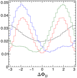
Building EFT-sensitive observables usually follows certain features of the higher-dimension operators. As an example of such a construction, let us consider the vector boson scattering process with creation of an on-shell Higgs boson. The operators , , and give rise to the -odd amplitudes in the interaction. The azimuthal angle between the two associated jets is an observable sensitive to these amplitudes [6], as illustrated in Fig. 1.
Observables optimized with matrix-element calculations
The idea of optimized observables was introduced in particles physics in Refs. [8, 9]. For a simple discrimination of two hypotheses, the Neyman-Pearson lemma [10] guarantees that the ratio of probabilities for the two hypotheses 0 and 1 provides an optimal discrimination power. For a continuous set of hypotheses with an arbitrary quantum-mechanical mixture of two states, one could apply the Neyman-Pearson lemma to each pair of points in the parameter space, but this would require a continuous, and therefore infinite, set of probability ratios. However, equivalent information is contained in a combination of only two probability ratios, which can be chosen as two optimized observables [11]
| (4) | |||
| (5) |
where the index of the probability density is discussed in application to Eq. (2). The constant is introduced for convenience and could be set to when symmetric appearance is desired, and these observables can also be defined with . The information content of the two observables used jointly is the same for any fixed value of , and the observable optimized for discrimination between two arbitrary hypotheses can be written as a function of and . In the case of a small contribution of to differential cross section, Eq. (5) with reproduces the optimal observable defined in Ref. [9].
Equation (2) allows us to make several important observations. When interference terms are absent, as for example in the case of non-interfering background, the optimized observables are of the type defined in Eq. (4). There is one optimized observable to separate signal from background, assuming background does not depend on EFT parameters. When interference is present and there are only two types of couplings with , there are only two optimized observables defined in Eqs. (4) and (5), as stated above. This illustrates the power of the multivariate techniques when the full information contained in the high-dimensional space of can be preserved in just two observables. This power is limited to the measurement of one parameter , though. However, when multiple couplings are present with , the number of optimized observables grows significantly as . At the same time, one can observe that for the purpose of an EFT measurement, the last two terms in Eq. (2) are quadratic in non-SM couplings and can be neglected. This leaves linear terms, describing interference with the SM amplitude, in the coupling expansion. The observables, one for each term of the type defined in Eq. (5) with , can be picked for optimal separation in an EFT analysis. Alternatively, the observables, one for each term of each of the types defined in Eqs. (4) and (5) with any fixed value of , will define the complete set of optimized observables.
Calculation of optimized observables as probability ratios in Eqs. (4) and (5) can be performed with the help of the matrix-element calculations in Eq. (1). The transfer functions introduced in Eq. (1), , are required for proper probability calculations. However, as opposed to the matrix element method discussed in Section 0.2.3 where the transfer functions have to be modeled fully, in the case of probability ratios certain effects cancel, and in any case, any imperfection does not bias the result, but only reduces optimality somewhat. Therefore, the transfer functions can often be omitted, with only minor effect on optimality, in cases where the process is fully reconstructed with good enough resolution.
While multiple operators usually contribute to each process, it is often possible to isolate a small number of operators that are preferably constrained in a given process. Other operators may be much better constrained elsewhere. It is also important to pick the correct basis, or rotation, of the operators, in which blind or weak directions are removed. When such a situation is possible, the matrix-element calculations provide a prescription for calculating the observables optimal for EFT measurements. Therefore, before a measurement can be attempted, one must obtain a map of processes and operators with the weak directions resolved.
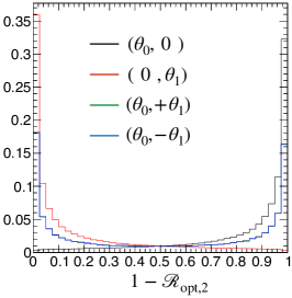
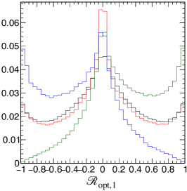
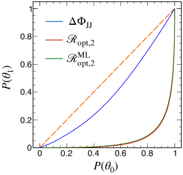
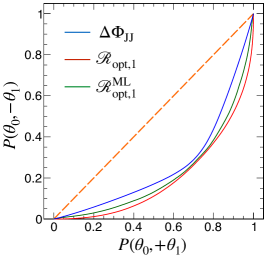
Examples of the and observables for the Higgs boson production in the and fusion can be found in Fig. 1 [7], and compared to the EFT-sensitive observable in this process . Among the three operators, , , and , there are two weak directions, corresponding to the and couplings, which are eliminated in the mass eigenstate basis. The separation power can be quantified with Receiver Operating Characteristic (ROC) curves, shown in Fig. 2. Performance of the observable is validated with two samples corresponding to the and models. For a given selection threshold, a point with probabilities to select events from either one model or the other samples the ROC curve. In a similar manner, performance of the observable is validated with two samples corresponding to the and models. The two models differ only by the sign of interference, and therefore the interference component is emphasized in this test. Observables optimized with matrix element calculation exhibit the best performance in isolating the operator of interest.
Observables optimized with machine learning
While the matrix-element calculations guarantee optimal performance from first principles, there are practical limitations to their applications. The most critical limitations are the transfer functions, which are difficult and time-consuming to model. Parton shower and detector effects may confuse and distort the input to matrix elements to such a degree that calculations become impractical. Machine-learning techniques may come to the rescue in such a case. Training of machine-learning algorithms is still based on MC samples utilizing the same matrix elements that would be used for optimal discriminants discussed in Section 0.2.1. However, these MC samples reflect the parton shower and detector effects, and therefore allow construction of optimized observables which incorporate these effects.
There are two important aspects in this training: which observables should enter the learning process and which samples should be used. Matrix-element approach gives answers to both and provides insight into the process of constructing the optimized observables with machine learning. First, the input observables should provide full information , which could be simply the four-vectors of all particles involved, like in the matrix elements, or better derived physics quantities which are equivalent to those. Second, there are two types of optimal observables, as pointed in Eqs. (4) and (5). The first observable corresponds to the classic problem of differentiating between two models, and a machine-learning algorithm is trained on two samples corresponding to models and . The resulting observable is equivalent to Eq. (4). Training of the second discriminant is less obvious, as it is expected to isolate the interference component. A discriminant trained to differentiate the two models with maximal quantum-mechanical mixing and becomes a machine-learning equivalent to that in Eq. (5) [7].
Performance of the two optimized observables and obtained with machine learning (Boosted Decision Tree in this case) is illustrated in Fig. 2 for the same example discussed in Section 0.2.1. Since only acceptance effects were introduced in MC simulation for illustration purpose, and those cancel in the ratios in Eqs. (4) and (5), the matrix-element and machine-learning optimized observables exhibit the same performance. There is a small degradation in performance of the , which is attributed to the more challenging task of training in this case and should be recovered in the limit of perfect training.
This Section provides a straightforward path to observables optimized with machine learning. A more elaborate approach to inference with machine learning is discussed in Section 0.2.3.
0.2.2 Approaches to experimental measurements
The ideal situation in Eq. (1) would be , which means that the truth-level quantities could be reconstructed in experiment without any loss of information and . This never happens in practice, and experimental techniques are needed to analyze the data. In experiment, the distribution is observed, and it is matched to the predicted distribution in order to obtain the confidence intervals of . There are two conceptually different approaches taken in particle physics to use Eq. (1) for the measurements:
-
•
In the single-step approach, the observed distribution is matched directly to the reconstruction-level prediction to obtain constraints on .
-
•
In the two-step approach, first the distribution is unfolded and the best approximation to the truth-level distribution is reported, where is a reduced set of quantities describing the truth-level process. In the second step, the observed unfolded distribution is matched to the truth-level prediction to obtain constraints on .
In the above, is a subset of in Eq. (1) which matches the as close as possible. It does not have to be complete and may represent just one quantity, e.g. the invariant mass of a system. The parton-level prediction for a reduced set of quantities can be expressed as
| (6) |
where integration is performed over the degrees of freedom not used in differential distributions.
The two approaches have their pros and cons and both have been widely utilized in particle physics. The single-step approach is conceptually straightforward and unbiased, if modeling of the effects in Eq. (1) is done correctly, e.g. with MC simulation. It may also be the most optimal approach, if the choice of observables is optimal and contains the full information as close to as possible. However, this approach suffers from two main drawbacks, which are complementary to the two-step approach discussed below. First of all, re-analysis of the data requires the full chain of experimental processing, starting from a modification of in Eq. (1) and MC simulation of experimental apparatus with the new model, e.g. after changing the list of EFT operators targeted in analysis as described by . For this reason, theoretical collaborations cannot easily reuse the results of such an analysis to adopt a new model. Second, this approach is rather complex because the EFT modeling should be done with the full detector simulation, and leads to a much more involved process than the analysis of unfolded distributions, which requires EFT modeling at parton level only.
The two-step approach is attractive for two main reasons: First of all, it allows wide dissemination and preservation of the data in the form of differential truth-level distribution for later re-analysis, e.g. by theoretical collaborations. Second, this approach decouples the experimental effects in the first step from analysis of EFT effects in the second step, which greatly simplifies the EFT part of analysis. These two features make this approach especially attractive for analysis of differential distributions outside of the experimental collaborations. At the same time, this approach suffers from two main drawbacks, which potentially may lead to a non-optimal and/or biased analysis. The choice of is usually limited to one or few observables, resulting in significant loss of information compared to the complete set . The unfolding from to depends on , but these parameters are not known in advance. The SM assumption is usually made in such unfolding, which may lead to bias. With multiple processes, background subtraction for a given process is also usually done assuming SM parameters in the other processes, which may also lead to bias.
While measurements in the single-step approach can enter the global EFT fit directly by building the joint likelihood of multiple measurements within experimental collaborations, reporting these measurements outside of such collaborations may represent a challenge. The usual practice of reporting multi-gaussian approximation may not be sufficient for proper combination with other measurements. The proper treatment requires that the experiments release the full likelihood associated to their measurement, which represents technical challenges, but possible in principle. Alternatively, the intermediate reco-level parameterization of a single-step approach could be reported, which would effectively lead to a two-step approach, but full information would be retained. In such a case, the observed distribution is reported by an experiment for a given observable , along with the expected distributions for a variety of models of interest , and including background processes. This approach shares pros and cons of the above two main approaches. This approach eliminates the unfolding procedure with its own complications and allows easy interpretation of public differential distributions. However, this approach still limits the re-interpretation to only those models which have been pre-computed with the tools used by the experiments. This approach also limits available information, as typically only 1D differential distribution of an observable is reported. However, the latter limitation could be overcome if several optimized observables are utilized simultaneously.
The dependence of the unfolding procedure on the EFT parameters can be illustrated with the following. Eliminating from Eq. (1) leads to an equivalent expression
| (7) |
with a very important difference in comparison to Eq. (1): the modified transfer function
must, in general,
depend on the model parameters . This dependence becomes pronounced if
detector effects are not uniform and distributions
vary with over the degrees of
freedom .
A curious reader can confirm this conclusion by deriving the expression for
,
which is a non-trivial function of in the case of non-trivial detector effects.
The reverse transformation of Eq. (7) becomes the unfolding procedure, which is discussed in Section 0.2.3. The dependence of unfolding on the model parameters creates challenges in the EFT interpretation. This is usually sidestepped by assuming SM parameters in the transformation
| (8) |
where the level of approximation in Eq. (8) with the assumption needs to be reported for the range of parameters under consideration. In practice, modeling of Eq. (8) is performed with MC simulation of the SM processes, and the level of approximation needs to be tested with alternative simulations, including detector effects, for a range of . Ideally, experimental collaborations should also report prescription for correcting the bias for certain popular models with parameters . These corrections are particularly important to evaluate for modification of EFT parameters because they can lead to dramatic detector effects, e.g. very different response due to substitution of and particles in the propagators.
The choice between the single-step vs. the two-step approaches to experimental measurements is driven by the tradeoff between the various pros and cons and by the available resources, data, and tools. The single-step approach is the most optimal and can use the full knowledge of detector information, and therefore it is most suitable for analysis by the experimental collaborations. The two-step approach is easier for re-interpretation, even if this comes at the cost of some loss of information and potential bias, and therefore it is most suitable for analysis by the theoretical collaborations without access to detector information.
In the end, experimental measurements are experimentally delivered quantitative results, which are typically cross sections or related quantities, and can be further used in global fits for EFT parameters . (Applications of experimental measurements to global EFT fits are discussed in Area 4 of the group effort.) These experimental measurements are obtained from analysis of observables in a limited set of processes. We group experimental measurements sensitive to EFT effects in several categories, which progress from simple to more involved:
-
•
single-process cross section;
-
•
single observable differential distribution affected by a single or multiple processes;
-
•
multi-observable differential distribution or multiple single-observable differential distributions with correlations;
-
•
binned sub-process cross sections, such as STXS (Section 0.2.3) in Higgs boson physics;
-
•
dedicated EFT measurements, such as amplitude analysis with cross sections per EFT operator;
-
•
dedicated EFT operator extraction by experiments.
The first four types of measurements can be generically called differential and fall under the two-step approach. The last two types of measurements can be generically called dedicated and fall under the single-step approach. All of the above types of measurements can be either analyzed stand-alone or enter combination with other measurements in the global fits.
0.2.3 Statistical methods for experimental measurements
We discuss further ingredients of experimental measurements, such as unfolding techniques for calculation of differential distributions , and likelihood-based and likelihood-free inference techniques.
Unfolding
Unfolding or signal deconvolution is a broad term that refers to techniques that seek to translate data from one form, which contains noise or distortions, into another, which does not. In the context of High Energy Physics, this usually refers to correcting experimental data for detector acceptance, efficiency, and resolution effects. The reconstructed data (colloquially referred to as the reco level) is corrected for the effects of the detector to the truth level. This is equivalent to inverting the transformation in Eq. (8) to convert the observed distribution of events into the distribution at truth level . As discussed at the beginning of Section 0.2, the truth level can refer to any set of observables that are defined based on information in the MC event record, the particle level or parton level.
The results that are unfolded are almost always binned data presented in histograms. Therefore, unfolding is, at its essence, a matrix inversion problem. All unfolding techniques rely on construction a matrix that maps truth events in bin to reco events in bin which is usually called a response matrix or a migration matrix. A general representation of unfolding is given by:
| (9) |
where is the observable to be unfolded, is the integrated luminosity of the data, is the branching ratio of the channel being studied, is the width of the bin in observable , is the number of observed events in data in bin , is the number of expected background events in bin . is the response matrix, is a bin-by-bin correction factor that accounts for the limited phase-space of the event selection (sometimes called an extrapolation correction, and is a bin-by-bin correction factor that accounts for reco events that are not present in the truth selection (sometimes called non-fiducial backgrounds). Most unfolding techniques work by inverting and applying that inverted matrix to the observed data to remove detector effects. Matrix inversion is a well-studied problem and, in the context of unfolding, the main challenge is to control harmonic fluctuations in the statistical uncertainties that are inherent to the process of inverting the response matrix. The key difference between different unfolding approaches are usually how these statistical uncertainties are controlled (a process often called regularisation). For example, in Iterative Bayesian Unfolding [12], these fluctuations are regularised using an iterative technique based on Bayes theorem, whereas in Singular Value Decomposition [13] the technique for which it is named is used to control the statistical fluctuations.
An aside on notation
Experimental collaborations are not consistent in the notation used in unfolded results, both within and without, and great care must be taken to understand exactly how each result has formulated the unfolding problem. Equation 9 is a fair representation of the most factorised form of the general unfolding problem. However, some results may concatenate various aspects. For example, the matrix may sometimes have the effects of and folded in, or the denominator in the first fraction can be combined into a single factor. Experimental results also use the terms response and migration matrix interchangeably and inconsistently so the specific definition in each result must be taken into account.
Using unfolded results in EFT fits
All unfolded results are, by definition, biased. The techniques that are used to tackle the matrix inversion problem, as well as to control for other experimental effects, invariably introduces some dependence on the model used to construct them, as discussed in reference to Eqs. (7) and (8). However, it is not true to say that this bias is always large or prohibits the use of results in EFT fits. It is more correct to say that unfolded results have a region of validity centred on the SM but which extends beyond it. How far that model extends, and in particular if it extends sufficiently far to encompass shifts in various Wilson Coefficients, depends on a number of things. The most important components to consider when using unfolded results in EFT fits are , , , and . in its simplest form (i.e. without the factors folded in) is usually the same regardless of the model used to build it as it is only probing the detector smearing effects. Matrices that are highly diagonal and symmetric about the diagonal, are likely to have a much broader region of validity than, say, a matrix that is diagonal but off-centre and which has significant one-sided smearing. is an extrapolation out of the phase space of the measurement and into some other phase-space, usually that of the total cross-section. It is entirely dependent on the model that constructs it. However, it can easily be undone post-hoc and redone with EFT effects included, and is therefore not a huge problem when considering EFT fits. cannot be redone post-hoc and is also somewhat dependent on the model used to construct it. In cases where this is flat and close to one, the bias that it causes is negligible (especially for normalised differential cross-sections). However, significant shapes in this curve is usually an indication that the region of validity of the result is small. Finally, is only problematic for EFT fits if the background is non-negligible and could be effected by the Wilson coefficients under study. Such effects can usually be avoided by only selecting results with high signal purity, such as Drell-Yan, top quark, and dijet results, though this is not an exhaustive list.
Recommendations for unfolded results
The safest results to use in EFT fits have the following properties:
-
•
They have a very high signal to background ratio and, ideally, what backgrounds to penetrate the signal region are not sensitive to the Wilson coefficients being probed.
-
•
They have highly diagonal response matrices and/or response matrices which are highly symmetric about the diagonal which makes the detector smearing effects marginal and well-controlled.
-
•
They have flat curves. This is especially relevant for normalised differential cross-sections, as it means the shape of the unfolded data is decoupled from the normalisation and therefore safe to use in an EFT fit where the shape of the EFT effects is very different from the SM.
-
•
They are measured in a tight fiducial region and at particle level (which, by extension, means that should be close to unity and flat.)
There are relatively few experimental results that satisfy all of these criteria (though, unfolded angular observables are usually ideal) and omitting one or more of these recommendations is reasonable as long as some considerations for the effect of the bias on any fits is considered in more detail.
Simplified template cross sections

In the analysis of the Higgs boson data on LHC, a framework of the simplified template cross sections (STXS) [15] has been developed, which is designed for the measurement of the single- cross sections in mutually exclusive regions of the phase space (which includes parton shower in this case). The observable quantities are the bins of kinematic templates for each Higgs boson production process. An example of such a template is shown in Fig. 3 for the electroweak production of the Higgs boson in association with two jets, where ten bins are defined based on the quantities characterizing the process. These bins have been chosen to provide sensitivity to higher-dimension operators, which typically exhibit enhancement at higher transverse momenta.
This framework falls under the two-step measurement approach discussed in Section 0.2.2 and shares its pros and cons. It resembles the differential distributions with the unfolding procedure discussed in Section 0.2.3, but has its unique features, and for this reason we discuss it in a separate section. This framework takes advantage of the fact that characterization of the Higgs boson production is independent from its decay. Therefore, the same quantities in STXS are measured with multiple Higgs boson decay channels. At the same time, the production processes are separated during the data analysis and results are presented for each production process independently, which is different from the typical Higgs boson differential distributions. These features are unique to Higgs boson physics and for this reason this framework has not found application in other areas so far. The main advantage of this approach is wide dissemination of results for (re)interpretation in a uniform way. The main disadvantage is its limited scope and potential dependence of cross section interpretation on the parameters of the model, as discussed in reference to Eqs. (7) and (8).
Template likelihood fit
The end goal of most analyses on LHC is to construct the likelihood and maximize it to obtain the best-fit values of and set their confidence intervals. This approach can be taken either in the single-step approach, when EFT-sensitive parameters are measured directly, or in the two-step approach, when intermediate cross sections are measured, e.g. in the STXS approach. There are various techniques to construct or approximate the likelihood, including the matrix element method and machine learning, discussed below, but the most straightforward and widely used approach is the so-called template approach.
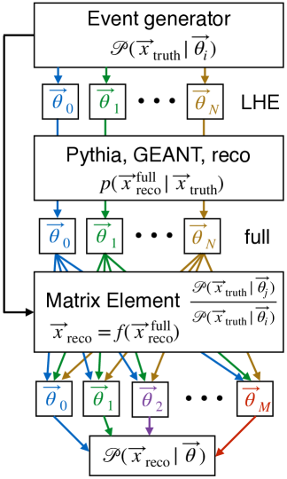
In the template approach, the pdf is a histogram, or template, of observables binned in one or several dimensions. The dependence on parameters in the special case of EFT couplings is shown in Eq. (2). This allows analytical morphing of template parameterization by generating a discrete number of models corresponding to each term in Eq. (2). Construction of such templates is illustrated in Fig. 4, where the chain of MC modeling of the pdf follows Eq. (1). An event generator produces LHE files [16] for hypotheses , which are processed through full MC simulation, including parton shower and detector effects. It is important to pick a diverse enough set of hypotheses in such a way that all corners of phase space are sampled well. However, this set does not need to be complete, as matrix element re-weighting of MC samples allows generating any number of models . This last step of re-weighting is a lot less time consuming than the full MC simulation. Therefore, in order to minimize statistical uncertainties at minimal cost, any model can be re-weighting to any other model. In the end, constraints could be obtained on and the overall cross section of the process.
Matrix element method
The matrix element method (MEM) employs Eq. (1) directly to construct a likelihood function. It is important to draw distinction between MEM, discussed in this section, and the observables created with the help of matrix-element calculations, discussed in Section 0.2.1. In the latter case, matrix elements are used to calculate observables following the general approach of Eq. (3). These observables can later be used in different measurements, from differential distributions to machine-learning inference. The MEM approach, on the other hand, is the direct way to perform a measurement through construction of a likelihood with the help of transfer functions .
The MEM approach is particularly suited to EFT measurements for two main reasons. First of all, such an approach may be built close to optimal because nearly the full information can be employed. Second, the large number of EFT parameters can be easily incorporated in this approach because those appear in the readily available matrix element calculation . In other words, once the transfer functions are incorporated, there is no limitation on the matrix element calculations, other than availability of the matrix elements themselves. Once a MEM analysis is built for the SM process, it can easily be extended to EFT by plugging in the right matrix elements.
At the same time, the MEM approach has its own limitations. The first challenge is to build the transfer functions , which is never possible to do from first principle and certain approximations have to be employed. This becomes particularly challenging in the case of high multiplicity of particles generated in parton shower and considered in analysis. Correct particles could escape detection, wrong particles could be picked, and permutations of particles could create confusion. Therefore, the MEM approach is most successful when full reconstruction of the process with little confusion is possible. The second challenge is computational, as numerical technics for calculations and integration often have to be employed and would lead to significant CPU requirements. The MEM approach is most successful when a large degree of analytical calculations could be maintained. The third challenge is availability of the matrix elements for all processes considered. In particular, not all background processes could be described analytically, such as instrumental background. One may approximate such backgrounds either with empirical functions or templates of observables. However, the former is not necessarily possible and the latter eliminates some of the main advantages of the MEM approach.
The first proposal of MEM in application to a non-trivial environment of hadron collisions with missing particles was made in Ref. [18]. There have been a number of successful applications of the MEM approach to the Higgs, top, electroweak, and -quark flavor measurements at LHC and other experiments. At the same time, the MEM approach has not become the main approach in performing the measurements on LHC due to its challenges.
Inference with machine learning
The heart of the challenge for inferring the EFT parameters from data is that the likelihood function defined by Eq. (1) involves an intractable integral. As expressed in Eq. (1) even the transfer function is intractable as it would involve an enormous integral over the truth-level quantities that describe the parton shower, hadronization, and the electromagnetic and hadronic showers that occur when final state particles interact with the detector. We introduce to denote the full MC truth record that includes the hard scattering as well as the other steps in the full simulation chain, and use it interchangeably with . In the language of statistics and machine learning, our simulation chain is a generative model and all the random variables in the MC simulation that we refer to as MC truth are referred to as latent variables. Simulators like this that can be used to generate synthetic data with MC, but which do not admit a tractable likelihood are referred to as implicit statistical models [19].
The task of performing statistical inference when the data generating process does not have a tractable likelihood is known as simulation-based or likelihood-free inference [20]. This case is not at all unique to particle physics. The formulation of this problem in a common, abstract language has led to statisticians, computer scientists, and domain scientists from various fields developing powerful methods for simulation-based inference together.
The particle physics community has been coping with problems like this for decades. The strategy is to use histograms or kernel density estimation to approximate the intractable integral from samples of synthetic data generated with MC. Since it is not practical to histogram the high dimensional data , we identify observables (summary statistics) that carry as much information about the parameters as possible. This is the well known template likelihood fit strategy, discussed in Section 0.2.3. Alternatively, the matrix element method, discussed in Section 0.2.3, seeks to approximate through numerical integration, but must rely on a simplification of the transfer function that does not involve the details of the parton shower and detector interaction. However, machine learning opens up new ways to approximate the likelihood function that does not require sacraficiing power with the introduction of summary statistics nor does it require a simplification of the transfer functions that one would obtain with the full parton shower and detector simulation and reconstruction.
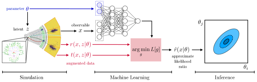
A schematic of this approach is shown in Fig. 5. A parametrized neural network [22, 23] is used to learn the likelihood ratio , where is some reference distribution such as the SM or a potentially unphysical mixture of different EFT points. The choice of this reference distribution simply leads to an offset in the log-likelihood and does not affect the maximum likelihood estimate or the resulting contours. The reason that the reference distribution is used is that it allows us to reframe the task of approximating the likelihood from one of density estimation to classification. We can train a parametrized neural network on the supervised learning task of binary classification between data generated from and data generated from . Instead of using a different neural network for each EFT parameter point, a single parametrized network learns to interpolate.
The most basic version of this approach was first laid out in Ref. [22], but generating MC training samples that cover the full EFT space is prohibitive. Furthermore, in the region of the EFT space we are most interested in, the deviation from the SM prediction is small. This means that in the two samples the classifier is trying to distinguish two distributions that are nearly the same, which leads to a poor approximation of the likelihood ratio. Both of these challenges can be overcome [21, 24]. The first point is that the analytical morphing allows us not only to morph template histograms but also to continuously reweight individual events [25]. Together with a resampling procedure, we can produce training data that uniformly covers the EFT parameter space from a finite number of basis samples. References [21, 24, 26] also describe how the analytical morphing can be used to encode the dependence directly into morphing-aware neural network architectures. However, these tricks do not address the problem that the deviation from the SM is small. This is addressed by a trick known as mining gold [27, 28]. The insight here is that while involves an intractable integral, the joint likelihood ratio and the joint score are tractable because the terms that depend on the transfer functions drop out when the -dependence is isolated to the hard scattering. Moreover, both of these quantities can be computed directly from the analytic morphing equations. These can then be used to augment the training data and lead to dramatically more efficient training. The joint score in particular is of interest because it is a local quantity and directly characterizes how much more or less likely it would be for a region of phase space to be populated if the EFT parameters were modified from their SM values. By regressing on these quantities it is possible to recover the likelihood ratio or the score (having marginalized out the latent variables associated to MC truth). It turns out that the score function provides locally sufficient statistics, coincides with the concept of optimal observables when detector effects are negligible, as introduced in Section 0.2.1, and generalizes them to settings where detector effects must be taken into account, as shown in Section 0.2.1. The software package MadMiner [29, 30] provides a reference implementation of these techniques.
0.3 Operators and measurements for global SMEFT fits
One of the goals of this activity area on Experimental Measurements and Observables is to survey which experimental channels are sensitive to which EFT operators. The aim is to establish a map between operators and experimental measurements. As a first step we want to determine which operators are relevant and as a second step to examine the amount of information that each process can provide for a given operator, given the accuracy of any given experimental process. The second step can be achieved by considering some appropriate metric such as the Fisher information.
A valuable source of information in this endeavour are the global fits which exist in the literature.
The set of operators relevant for each fit is determined by the processes included in the fit as well as the choice of
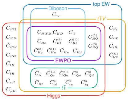
flavour assumption which determines the relevant degrees of freedom. As an example, in Fig. 6
we show a schematic representation of the datasets and their overlapping dependences on the 34 Wilson coefficients
included in the global Higgs, top, diboson and EWPO analysis of fitmaker [31].
A major part of global interpretations of HEP data in the SMEFT framework is establishing the connection between operators and experimental measurements and eventually the generation of predictions for the dependence of each measurement on the Wilson Coefficients of interest. The first step involves starting from a particular flavour assumption and then creating a list of operators entering a given process at some perturbative order. The second step is more quantitative and typically involves a significant undertaking, requiring large scale numerical calculations that take into account details of the experimental analyses. The map from operators to measurements contains a great deal of information in itself, indicating both how the data may collectively constrain each degree of freedom and the origin of potential correlations among them, post-fit.
Such results only make up half of the required ingredients of a global fit, the other half being the experimental data and covariance matrix. Nevertheless, it is worthwhile to present and dissect them in a systematic way for a number of reasons. From a fundamental perspective, we may understand the potential impacts and interplay that the data imposes on the allowed parameter space of the theory, which can guide our expectations before doing any elaborate fits and also help us to understand the results of such an exercise. Moreover, it serves as a useful validation exercise, where we can verify the consistency of the predictions both internally and against other existing calculations. This is especially important given the fact that such a large scale generation of predictions is inevitably prone to human error. Finally, making the results public allows them to be re-used in future interpretations, avoiding a duplication of effort and therefore hastening progress towards maximal indirect sensitivity to new physics from precision measurements.
In this note, we establish a map between operators and experimental measurements and quantify the sensitivity of the Higgs, top, and Electroweak measurements that went into the recently published global analyses of fitmaker [31] and SMEFiT [32] collaborations. Whilst the two collaborations follow similar approaches, some differences exist and these will be mentioned in the note where relevant.
0.3.1 Calculational framework
In this note we work in the Warsaw basis of SMEFT dimension-6 operators [33]. The operator coefficients are normalised as
| (10) |
Before discussing the operators entering each analysis we briefly
mention the corresponding flavour assumptions as employed by the
two fitting collaborations. SMEFiT [32] follows the strategy presented
in [34, 35], namely
minimal flavour violation (MFV) hypothesis [36] in the
quark sector as the baseline scenario.
fitmaker [31] considers both a flavour universal
and an MFV scenario. We discuss in detail the operators considered in each analysis below.
Operator basis in SMEFiT 2021 analysis
The SMEFiT analysis adopts a symmetry where the Yukawa couplings are nonzero only for the top quark, consistent with the SMEFT@NLO model [37]. Whilst strictly not consistent with the flavour assumption, the bottom and charm quark Yukawa operators are included in the fit, to account for the current LHC sensitivity to these parameters, while all other Yukawas are set to zero. A universal symmetry is adopted in the lepton sector, which sets all the lepton masses as well as their Yukawa couplings to zero. Again, a non-zero Yukawa operator is allowed.
| Class | Independent DOFs | DoF in EWPOs | |
|---|---|---|---|
| four-quark | 14 | , , , | |
| (two-light-two-heavy) | , , , | ||
| , , , | |||
| , , , | |||
| , | |||
| four-quark | 5 | , , , | |
| (four-heavy) | , | ||
| four-lepton | 1 | ||
| two-fermion | 23 | , , , | , , |
| (+ bosonic fields) | , , , | , , , | |
| , , , | , , , | ||
| , , | |||
| , | |||
| Purely bosonic | 7 | , , , | , |
| , | |||
| Total | 50 (36 independent) | 34 | 16 (2 independent) |
| Operator | Coefficient | Definition |
|---|---|---|
With this considerations, one ends up with 50 dimension-six EFT degrees of freedom to be constrained by experimental data. These are summarised in Table 1, categorised into five disjoint classes, from top to bottom: four-quark (two-light-two-heavy), four-quark (four-heavy), four-lepton, two-fermion, and purely bosonic DoFs. Flavour indices are labelled by and ; left-handed quark and lepton fermion SU(2)L doublets are denoted by , ; the right-handed quark singlets by , , while the right-handed lepton singlets are denoted by , , without using flavor index. We use and to denote the left-handed top-bottom doublet and the right-handed top singlet, and the Higgs doublet is denoted by . Of these 50 EFT coefficients, 36 are independent fit parameters while 14 are indirectly constrained by the LEP EWPOs, following the procedure described in [32].
When presenting results for operator sensitivity, the SMEFiT analysis selects the purely bosonic operators and , for illustration purposes.
Table 2 provides the definition of the purely bosonic dimension-six operators considered in the analysis, which modify the production and decay of Higgs bosons as well as the interactions of the electroweak gauge bosons. In addition to the information provided by the input dataset, the operators and are also severely constrained by the EWPOs. The triple gauge operator generates a TGC coupling modification which is purely transversal and is hence constrained only by diboson data.
Table 3 collects, using the same format as in Table 2, the relevant Warsaw-basis operators that contain two fermion fields, either quarks or leptons, plus a single four-lepton operator. From top to bottom, the table lists the two-fermion operators involving 3rd generation quarks, those involving 1st and 2nd generation quarks, and operators containing two leptonic fields (of any generation). In this list the four-lepton operator is also included. The operators that involve a top-quark field, either (left-handed doublet) or (right-handed singlet), are crucial for the interpretation of LHC top-quark measurements and all of them involve at least one Higgs-boson field, which introduces an interplay between the top and Higgs sectors of the SMEFT. We point out that most of the operator coefficients defined in Table 3 correspond directly to degrees of freedom used in the fit, except for three of them, which are indicated with a (*) in the second column, for which three additional degrees of freedom are defined from the linear combinations following [35], see [38].
| Operator | Coefficient | Definition |
| 3rd generation quarks | ||
| (*) | ||
| (*) | ||
| 1st, 2nd generation quarks | ||
| (*) | ||
| two-leptons | ||
| four-lepton | ||
Finally, SMEFiT considers four-quark operators which involve the top quark fields and thus modify the production of top quarks at hadron colliders. These can be classified into operators composed by four heavy quark fields (top and/or bottom quarks) and operators composed by two light and two heavy quark fields. The EFT coefficients are constructed in terms of suitable linear combinations of the four fermion coefficients in the Warsaw basis,
| (11) | ||||
In Table 4 we provide the definition of all four-fermion EFT degrees of freedom that enter the fit in terms of the coefficients of Warsaw basis operators of Eq. (11). Recall that within our flavour assumptions, the coefficients associated to different values of the generation indices () or () will be the same.
| DoF | Definition (in Warsaw basis notation) |
|---|---|
Operators in the fitmaker analysis
There are 20 operators relevant for Higgs, diboson and electroweak measurements in the flavour universal scenario. In the notation of Ref. [33], these are
| (12) | |||
| (13) |
We note here the slightly different notation used as denotes the Higgs doublet for which Tables 1 and 3 use a . Otherwise, the above operator choice corresponds to a subset of the SMEFiT operators with the following differences:
-
•
is equivalent to in SMEFiT up to a minus sign from integration-by-parts
-
•
and the SMEFiT differ by a conventional minus sign
-
•
fitmakeradditionally includes the muon Yukawa operator,
As mentioned, for the purposes of this note we focus on the Higgs, diboson and electroweak measurements, and relevant operators. We refer the reader to Ref. [31] for the global analysis, which also includes top physics measurements.
0.3.2 Experimental measurements
Input experimental data in SMEFiT 2021 analysis
We discuss next the experimental data used in [32]. In Table 5 we summarise the number of data points in the baseline dataset for each of the data categories and processes considered in this analysis, as well as the total per category and the overall total. SMEFiT include 150, 97, and 70 cross-sections from top-quark production, Higgs boson production and decay, and diboson production cross-sections from LEP and the LHC respectively in the baseline dataset, for a total of 317 cross-section measurements. For all processes, we consider only parton-level measurements, since the theoretical EFT interpretation and simulation of particle-level measurements is more challenging.
| Category | Processes | |
|---|---|---|
| Top quark production | (inclusive) | 94 |
| , | 14 | |
| single top (inclusive) | 27 | |
| 9 | ||
| , | 6 | |
| Total | 150 | |
| Higgs production | Run I signal strengths | 22 |
| and decay | Run II signal strengths | 40 |
| Run II, differential distributions & STXS | 35 | |
| Total | 97 | |
| Diboson production | LEP-2 | 40 |
| LHC | 30 | |
| Total | 70 | |
| Baseline dataset | Total | 317 |
Concerning top-quark production measurements, we consider four different categories: inclusive top-quark pair production, top-quark pair production in association with vector bosons or heavy quarks, inclusive single top-quark production, and single top-quark production in association with vector bosons. Top-quark pair production in association with a Higgs boson is considered part of the Higgs processes. The bulk of the top quark measurements corresponds to inclusive top-quark pair production, with measurements of single and double differential distributions in the dilepton and lepton+jets final states from ATLAS and CMS [39, 40, 41, 42, 43, 44, 45, 46, 47, 48, 49]. In general, the invariant mass distributions are found to be the most constraining observables. We also include top-quark pair charge asymmetry measurements: the ATLAS and CMS combined dataset at 8 TeV [50], and the ATLAS dataset at 13 TeV [51].
For associated top-quark pair production together with gauge bosons and heavy quarks, we consider the ATLAS and CMS measurements of the total cross-sections for and production [52, 53, 54, 55, 56, 57], in the ATLAS and CMS measurements of inclusive and production at 8 TeV and 13 TeV [58, 59, 60, 61, 62, 63]. In addition to inclusive measurements, we also consider the measurement of the differential distribution in production from CMS. The measurements are especially useful to constrain EFT effects that modify the electroweak couplings of the top-quark. We note that the and measurements can only be meaningfully described within a EFT analysis that accounts for the quadratic corrections.
In the case of inclusive single top-quark production both in the -channel and in the -channel, we account for total cross-sections and rapidity distributions from ATLAS and CMS [64, 65, 66, 67, 68, 69, 70, 71, 72]. We also consider the associated single top-quark production with weak bosons, with the and measurements from ATLAS and CMS at 8 and 13 TeV [73, 74, 75, 76, 77, 78, 79, 73, 80, 81].
Concerning Higgs boson production and decay measurements, we consider inclusive fiducial cross-section measurements (signal strengths) as well as differential distributions and STXS measurements. For the LHC Run I, we take into account the inclusive measurements of Higgs boson production and decay rates from the ATLAS and CMS combination based on the full 7 and 8 TeV datasets [82]. For the LHC Run II, we consider the ATLAS measurement of signal strengths corresponding to an integrated luminosity of fb-1 [83], and the CMS measurement corresponding to an integrated luminosity of fb-1 [84]. As in the case of the Run I signal strengths, we keep into account correlations between the various production and final state combinations.
In the case of differential measurements, we consider the ATLAS and CMS differential distributions in the Higgs boson kinematic variables obtained from the combination of the , , and (in the CMS case) final states at 13 TeV based on fb-1 [85, 86]. Specifically, we consider the differential distributions in the Higgs boson transverse momentum . We also include the ATLAS measurement of the associated production of Higgs bosons, , in the final state at 13 TeV [87]. Then we also include selected differential measurements presented in the ATLAS Run II Higgs combination paper [83]. Specifically, we include the measurements of Higgs production in gluon fusion, , in different bins of and in the number of jets in the event. Furthermore, we consider the differential STXS Higgs boson production measurements presented by CMS at 13 TeV based on an integrated luminosity of fb-1 and corresponding to the final state [88]. In all differential measurements, whenever available the information on the experimental correlated systematic uncertainties is included.
Finally we consider diboson production cross-sections measured by LEP and the LHC. To begin with, we consider the LEP-2 legacy measurements of production [89]. Specifically, we include the cross-sections differential in in four different bins in the center of mass energy, from GeV up to GeV. Concerning the LHC datasets, we include measurements of the differential distributions for production at 13 TeV from ATLAS [90] and CMS [91] based on a luminosity of fb-1. In both cases, the two gauge bosons are reconstructed by means of the fully leptonic final state. Our baseline choice will be to include the distribution for the ATLAS measurement, which extends up to transverse masses of GeV, while for the corresponding CMS measurement, the normalised differential distributions in is chosen. In addition, we also consider the differential distributions for production from ATLAS at 13 TeV based on a luminosity of fb-1 [92]. We note that diboson measurements are the only ones providing direct information on the triple gauge operator .
To finalise this discussion of the experimental data, we mention that the SMEFiT analysis framework was used in [38] for the EFT interpretation of vector-boson scattering (VBS) measurements from the LHC Run II, together with diboson data. The constraints on the electroweak EFT operators provided by VBS were found to be compatible with those derived in the global fit.
Input experimental data in fitmaker analysis
The fitmaker code contains a database of 342 measurements. We will consider here a subset pertaining to Higgs, diboson and electroweak precision data. fitmaker is publicly available such that the maps produced here can be extended to include Top data and different assumptions on the flavour structure.
The fitmaker dataset for the flavour universal scenario fit consists of the electroweak pseudo-observables reported by LEP/SLD, together with the mass measurements at ATLAS and Tevatron, a range of diboson measurements from LEP and ATLAS, as well as a large number of Higgs measurements, both inclusive and differential including STXS bins. It is constructed to avoid potential statistical overlap as much as possible, while favouring experimental combinations that provide access to correlation information. For example, only one type of Higgs measurement is included per experiment, i.e., an STXS combination for ATLAS and a signal strength combination for CMS, both of which publish correlation matrices. The datasets are further discussed below when the linear dependence of operators and measurements is presented. For more details, we refer the reader to Ref. [31]. This study precedes the latest CDF -mass measurement, and we refer interested readers to our recent dedicated study of the impact of this measurement in Ref [93].
0.3.3 Mapping between data and EFT coefficients.
In this section we discuss which operators enter which measurements following two different approaches. First we present the linear dependence of various measurements on the Wilson coefficients as presented in the fitmaker analysis. We then present the Fisher information table which determines the impact of various operators on different measurements taking into account the experimental precision.
Linear dependences of measurements on operators (Fitmaker)
In the fitmaker analysis the linear dependence, , on the Wilson coefficients, , is computed using MadGraph5 with the SMEFTsim UFO model for a measured quantity relative to the SM value ,
| (14) |
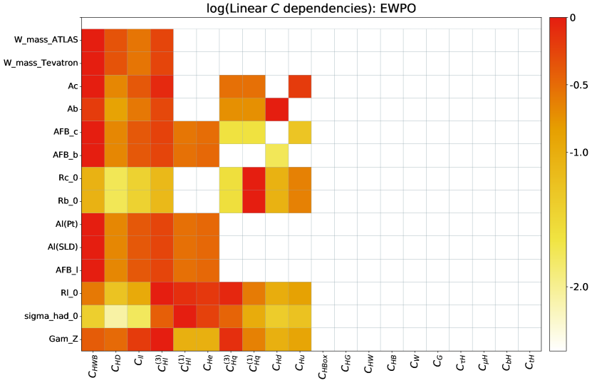
In other words, indicates the linear EFT cross-section for process and operator once the corresponding Wilson coefficient has been factored out. This is done at tree-level for all measurements except for the Higgs coupling to gluons which is calculated at one loop using SMEFT@NLO. Wherever relevant, measurements are of unfolded observables, such that the dependences are computed at parton-level in the unfolded phase space, not including any showering or detector effects. This means that using this set of dependences neglects any acceptance differences between the SM and the SMEFT predictions, which, in some cases, have been shown to be relevant (See, e.g., the impact of on the measurement of presented in Ref. [94]). See Ref. [31] for more details on our extraction of the linear dependences. After normalising the linear dependences of on the Wilson coefficients by dividing by the largest absolute value of the for a given measurement , the resulting normalised dependence is colour coded on a log scale in Fig. 7. Each row corresponds to a measurement while each column corresponds to a coefficient. The darkest red colours represent the strongest linear dependencies while the uncoloured white blocks indicate no dependence at linear order. We see that the right half of the grid is uncoloured since they correspond mostly to operators that can only be constrained in Higgs physics or diboson measurements. We can also read off that the operator coefficients most relevant for a large number of measurements is , though the operators and have the largest dependencies in the and asymmetries respectively. For the decay width, , it is the coupling to fermions modified by the operators corresponding to and that are the most important contributions to this measurement. It is well known that, of the 10 Warsaw basis operators that impact these measurements, only 8 linear combinations are actually constrained by a fit to this data alone [95].
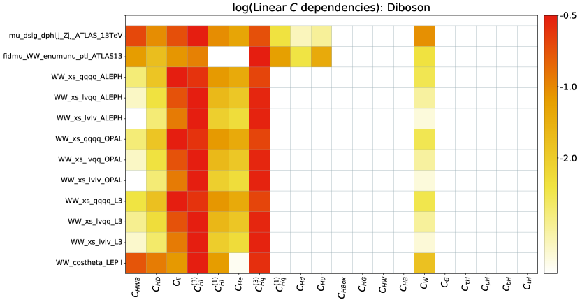
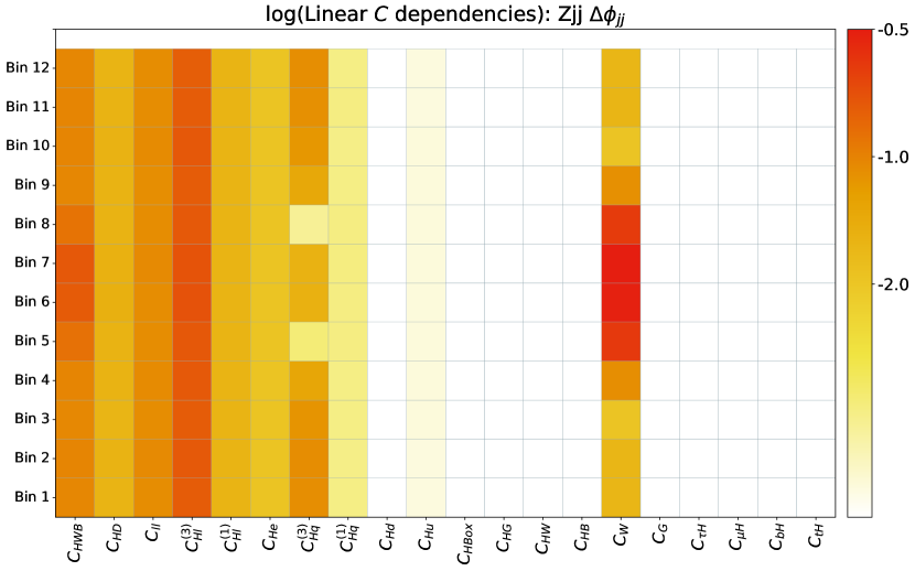
Similarly, Fig. 8 shows the mapping of linear dependences for a variety of diboson measurements in the same normalisation and colour scheme. These are differential distribution measurements that include either several kinematic bins or cross section measurements are different collider energy; we show here only the linear dependence in the last bin for simplicity. Just as in the decay width case, and are the largest contributions to these measurements. In this case, however, this is expected from the fact that these operators directly modify the interactions of the boson, while the others enter via -coupling modifications and input parameter shifts. Crucially, these measurements probe different linear combinations of the 10 operators constrained by the pole data. Moreover, we also see that the operator coefficient can now be constrained, in particular by the new data that was found by ATLAS to eliminate blind directions and be particularly sensitive to linear contributions from this operator in a global fit. Since the operator involves three gauge field strengths, it can only be constrained by diboson data and not by electroweak or Higgs processes. In Fig. 9 we show the linear dependences for all the bins of this differential measurement, where the linear dependencies are now normalised to 1 with respect to the strongest in all the bins. The non-trivial shape induced by is evident. This is in contrast to other, differential measurements such as boson ’s that suffer from a suppressed interference between the SM and that leads to relatively weaker sensitivity at linear level.
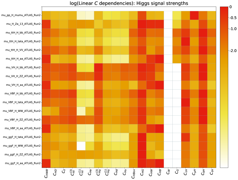
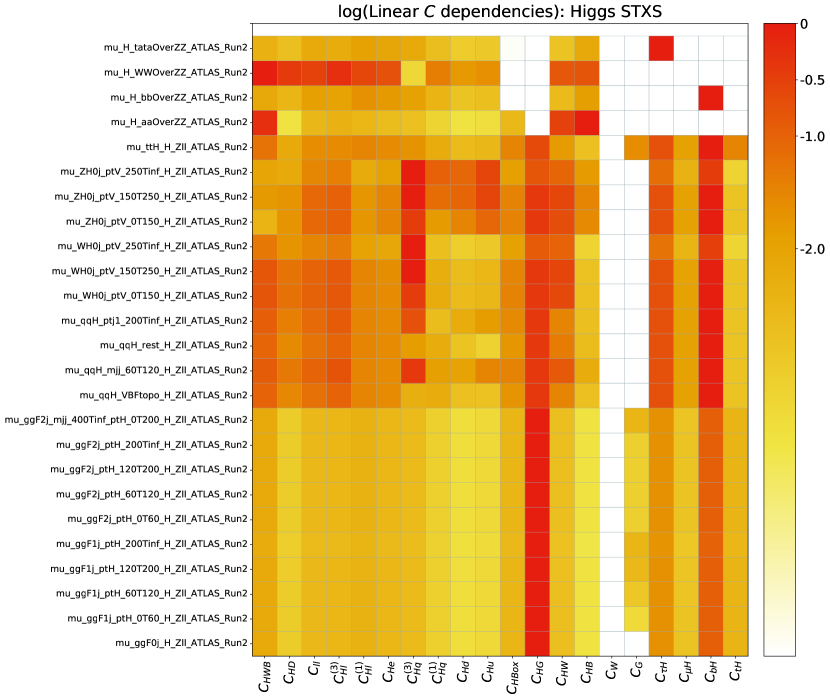
Finally in Figs. 10 and 11 are the maps for Higgs signal strengths and stage 1.1 Simplified Template Cross-section (STXS) bins, respectively. The operators that can only be constrained by Higgs physics are now populated. As expected, the gluon fusion channels depend on the strongest while the one-loop calculation using SMEFT@NLO [37] allows this to be properly calculated. This is also crucial to account for the effects of the triple gluon field strength operator coefficient, as well as the top quark chromomagnetic operator , which we considered in a generalised flavour assumption employed when combining with top quark data. The EW Higgs production modes provide additional handles on the current operators probed by the pole and diboson data. In general, the new kinematic granularity provided by the STXS bins breaks degeneracies among many operators present in the signal strengths.
Fisher information matrix analysis (SMEFiT)
A clean mapping between the input experimental measurements is provided by the tools underlying information geometry [96], specifically by means of the Fisher information matrix [32]. defined as
| (15) |
Here indicates the expectation value, is the functional dependence of the cross-section with the EFT coefficients and is the array of central experimental cross-section measurements. The functional dependence corresponds to the full likelihood function, which is most cases is provided as a multi-Gaussian distribution. It is important to emphasize however that the absolute size of the entries of the Fisher matrix does not contain physical information: one is always allowed to redefine the overall normalisation of an operator such that , with and with being arbitrary constants. For a given operator the relative value of between two groups of processes is independent of this choice of normalisation and thus conveys meaningful information. For this reason, in the following we present results for the Fisher information matrix normalised such that the sum of the diagonal entries associated to a given EFT coefficient adds up to a fixed reference value which is taken to be 100.
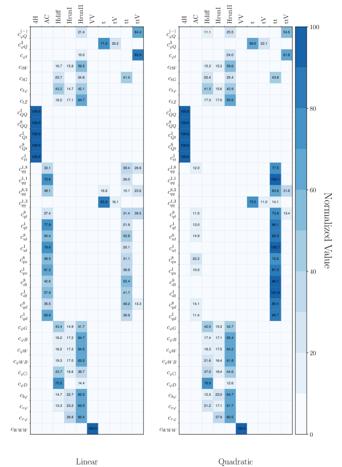
Fig. 12 displays the values of the diagonal entries of the Fisher information matrix both at the linear and at the quadratic level. We note that at linear order in the EFT expansion the dependence on the coefficients cancels out and the Fisher information matrix is strictly fit-independent. At the quadratic level one has some dependence on the Wilson coeffictions and the Fisher information needs to be computed in an iterative manner. One can identify, for each EFT coefficient, which datasets provide the dominant constraints. For instance, one observes that the two-light-two-heavy operators are overwhelmingly constrained by inclusive top quark pair production data, except for for which single top is the most important set of processes. At the linear level, the information on the two-light-two-heavy coefficients provided by the differential distributions and by the charge asymmetry data is comparable, while the latter is less important in the quadratic fits. In the case of the two-fermion operators, the leading constraints typically arise from Higgs data, in particular from the Run II signal strengths measurements, and then to a lesser extent from the Run I data and the Run II differential distributions. Two exceptions are , which at the linear level (but not at the quadratic one) is dominated by , and the chromo-magnetic operator , for which inclusive production is most important. Also for the purely bosonic operators the Higgs data provides most of the information, except for , as expected since this operator is only accessible in diboson processes. One observes that the corrections induce in most cases a moderate change in the Fisher information matrix, but in others they can significantly alter the balance between processes.
By fine-graining the calculation of the Fisher information matrix, one can gain insight about not only which group of processeses dominates the constraints on a given EFT coefficient, but also within a given group of processes which is the specific dataset that dominates. To illustrate this, tables 6, 7 and 8 display a similar comparison as that shown for Fig. 12 now in a fine-grained version and restricted to the inclusive top quark pair production datasets. Among various interesting observations, we see that in the quadratic EFT fit the constraints on the 2-light-2-heavy operators are dominated by the CMS measurements at 13 TeV in the dilepton and lepton+jets channels based on the 2016 dataset. This finding is not completely surprising, since these two datasets are the only ones based on 36 fb-1 of luminosity, yet it is reassuring that we can identify this dominance a priori, without needing to redo the actual fit.
| Processes | |||||
|---|---|---|---|---|---|
| Class | Coefficient | ||||
| 2FB | 0.000( 0.000) | 0.000( 0.000) | 0.000( 0.000) | 0.000( 0.000) | |
| 0.000( 0.000) | 0.000( 0.000) | 0.000( 0.000) | 0.000( 0.000) | ||
| 0.000( 0.000) | 0.000( 0.000) | 0.000( 0.000) | 0.000( 0.000) | ||
| 0.000( 0.000) | 0.000( 0.000) | 0.000( 0.000) | 0.000( 0.000) | ||
| 1.002( 0.976) | 3.025( 3.120) | 17.981( 18.770) | 10.349( 10.159) | ||
| 0.000( 0.000) | 0.000( 0.000) | 0.000( 0.000) | 0.000( 0.000) | ||
| 0.000( 0.000) | 0.000( 0.000) | 0.000( 0.000) | 0.000( 0.000) | ||
| 0.000( 0.000) | 0.000( 0.000) | 0.000( 0.000) | 0.000( 0.000) | ||
| 0.000( 0.000) | 0.000( 0.000) | 0.000( 0.000) | 0.000( 0.000) | ||
| 0.000( 0.000) | 0.000( 0.000) | 0.000( 0.000) | 0.000( 0.000) | ||
| 2L2H | 0.989( 0.116) | 0.910( 0.499) | 3.939( 2.715) | 2.907( 0.308) | |
| 0.746( -1.338) | 0.809( 0.769) | 0.594( 5.602) | 2.204( -4.524) | ||
| 0.568( -0.514) | 0.552( 0.335) | 2.638( 2.356) | 1.823( -1.572) | ||
| 0.000( -0.271) | 0.000( 0.440) | 0.002( 1.051) | 0.005( -0.862) | ||
| 0.968( -0.029) | 1.177( 0.662) | 6.098( 4.034) | 3.923( 0.290) | ||
| 1.008( -1.219) | 0.840( 0.749) | 0.584( 5.045) | 0.722( -4.150) | ||
| 1.324( -0.321) | 1.260( 0.987) | 4.812( 5.256) | 3.462( -0.637) | ||
| 0.466( -1.945) | 0.594( 1.070) | 0.815( 8.012) | 1.001( -5.962) | ||
| 1.741( -0.569) | 1.890( 1.267) | 10.610( 7.625) | 6.911( -0.784) | ||
| 0.516( -1.112) | 0.495( 0.704) | 0.870( 4.351) | 1.406( -3.318) | ||
| 1.722( -0.370) | 1.774( 0.678) | 7.789( 3.768) | 5.872( -1.217) | ||
| 0.803( -1.097) | 0.713( 0.770) | 2.627( 4.482) | 2.696( -4.220) | ||
| 2.681( -0.397) | 3.058( 2.103) | 13.187( 7.253) | 8.826( -1.971) | ||
| 0.610( -1.607) | 0.692( 0.845) | 1.493( 5.918) | 2.854( -5.613) | ||
| 4H | 0.000( 0.000) | 0.000( 0.000) | 0.000( 0.000) | 0.000( 0.000) | |
| 0.000( 0.000) | 0.000( 0.000) | 0.000( 0.000) | 0.000( 0.000) | ||
| 0.000( 0.000) | 0.000( 0.000) | 0.000( 0.000) | 0.000( 0.000) | ||
| 0.000( 0.000) | 0.000( 0.000) | 0.000( 0.000) | 0.000( 0.000) | ||
| 0.000( 0.000) | 0.000( 0.000) | 0.000( 0.000) | 0.000( 0.000) | ||
| B | 0.000( 0.000) | 0.000( 0.000) | 0.000( 0.000) | 0.000( 0.000) | |
| 0.000( 0.000) | 0.000( 0.000) | 0.000( 0.000) | 0.000( 0.000) | ||
| 0.000( 0.000) | 0.000( 0.000) | 0.000( 0.000) | 0.000( 0.000) | ||
| 0.000( 0.000) | 0.000( 0.000) | 0.000( 0.000) | 0.000( 0.000) | ||
| 0.000( 0.000) | 0.000( 0.000) | 0.000( 0.000) | 0.000( 0.000) | ||
| 0.000( 0.000) | 0.000( 0.000) | 0.000( 0.000) | 0.000( 0.000) | ||
| 0.000( 0.000) | 0.000( 0.000) | 0.000( 0.000) | 0.000( 0.000) | ||
| Processes | ||||||
|---|---|---|---|---|---|---|
| Class | Coefficient | |||||
| 2FB | 0.000( 0.000) | 0.000( 0.000) | 0.000( 0.000) | 0.000( 0.000) | 0.000( 0.000) | |
| 0.000( 0.000) | 0.000( 0.000) | 0.000( 0.000) | 0.000( 0.000) | 0.000( 0.000) | ||
| 0.000( 0.000) | 0.000( 0.000) | 0.000( 0.000) | 0.000( 0.000) | 0.000( 0.000) | ||
| 0.000( 0.000) | 0.000( 0.000) | 0.000( 0.000) | 0.000( 0.000) | 0.000( 0.000) | ||
| 0.939( 1.078) | 1.423( 1.579) | 3.431( 4.254) | 2.072( 2.486) | 1.207( 1.349) | ||
| 0.000( 0.000) | 0.000( 0.000) | 0.000( 0.000) | 0.000( 0.000) | 0.000( 0.000) | ||
| 0.000( 0.000) | 0.000( 0.000) | 0.000( 0.000) | 0.000( 0.000) | 0.000( 0.000) | ||
| 0.000( 0.000) | 0.000( 0.000) | 0.000( 0.000) | 0.000( 0.000) | 0.000( 0.000) | ||
| 0.000( 0.000) | 0.000( 0.000) | 0.000( 0.000) | 0.000( 0.000) | 0.000( 0.000) | ||
| 0.000( 0.000) | 0.000( 0.000) | 0.000( 0.000) | 0.000( 0.000) | 0.000( 0.000) | ||
| 2L2H | 1.003( 1.973) | 0.333( 0.560) | 8.035( 16.655) | 13.744( 39.714) | 7.522( 14.983) | |
| 1.441( 6.796) | 0.227( 2.201) | 9.698( 52.347) | 6.597( 34.891) | 3.678( 3.338) | ||
| 0.430( 2.986) | 0.130( 0.874) | 2.441( 37.461) | 0.937( 18.134) | 0.564( 3.590) | ||
| 0.001( 1.243) | 0.000( 0.420) | 0.007( 7.540) | 0.003( 4.673) | 0.002( -0.152) | ||
| 1.095( 3.119) | 0.401( 0.779) | 12.938( 43.148) | 3.043( 16.920) | 1.733( 4.893) | ||
| 1.148( 5.566) | 0.215( 1.966) | 10.525( 36.109) | 4.370( 36.495) | 2.456( 5.531) | ||
| 1.407( 5.182) | 0.377( 1.296) | 17.865( 40.618) | 7.932( 27.325) | 4.398( 3.189) | ||
| 0.878( 8.309) | 0.154( 3.035) | 6.966( 44.848) | 5.931( 40.126) | 3.270( 3.230) | ||
| 1.060( 4.667) | 0.670( 1.851) | 4.893( 43.891) | 2.067( 12.474) | 1.293( 2.146) | ||
| 1.523( 3.869) | 0.143( 1.609) | 20.696( 48.683) | 8.364( 26.455) | 4.580( 6.013) | ||
| 2.273( 4.198) | 0.779( 1.207) | 17.028( 44.740) | 9.665( 31.876) | 5.477( 9.261) | ||
| 1.816( 6.135) | 0.339( 1.948) | 16.044( 53.957) | 10.761( 35.154) | 5.924( 4.508) | ||
| 1.601( 3.070) | 1.207( 2.155) | 6.384( 32.430) | 7.078( 29.956) | 4.157( 5.835) | ||
| 2.438( 6.856) | 0.410( 2.536) | 18.526( 37.766) | 7.595( 36.886) | 4.297( 2.158) | ||
| 4H | 0.000( 0.000) | 0.000( 0.000) | 0.000( 0.000) | 0.000( 0.000) | 0.000( 0.000) | |
| 0.000( 0.000) | 0.000( 0.000) | 0.000( 0.000) | 0.000( 0.000) | 0.000( 0.000) | ||
| 0.000( 0.000) | 0.000( 0.000) | 0.000( 0.000) | 0.000( 0.000) | 0.000( 0.000) | ||
| 0.000( 0.000) | 0.000( 0.000) | 0.000( 0.000) | 0.000( 0.000) | 0.000( 0.000) | ||
| 0.000( 0.000) | 0.000( 0.000) | 0.000( 0.000) | 0.000( 0.000) | 0.000( 0.000) | ||
| B | 0.000( 0.000) | 0.000( 0.000) | 0.000( 0.000) | 0.000( 0.000) | 0.000( 0.000) | |
| 0.000( 0.000) | 0.000( 0.000) | 0.000( 0.000) | 0.000( 0.000) | 0.000( 0.000) | ||
| 0.000( 0.000) | 0.000( 0.000) | 0.000( 0.000) | 0.000( 0.000) | 0.000( 0.000) | ||
| 0.000( 0.000) | 0.000( 0.000) | 0.000( 0.000) | 0.000( 0.000) | 0.000( 0.000) | ||
| 0.000( 0.000) | 0.000( 0.000) | 0.000( 0.000) | 0.000( 0.000) | 0.000( 0.000) | ||
| 0.000( 0.000) | 0.000( 0.000) | 0.000( 0.000) | 0.000( 0.000) | 0.000( 0.000) | ||
| 0.000( 0.000) | 0.000( 0.000) | 0.000( 0.000) | 0.000( 0.000) | 0.000( 0.000) | ||
0.3.4 Impact of measurements on individual constraints (Fitmaker)
The linear dependence maps from measurements to Wilson coefficients provide important information to understand the result of a fit. However, the final constraint on a Wilson coefficient depends not only on how strongly a measurement varies with the corresponding coefficient but also on the sensitivity of those measurements. Some information in this direction is thus provide by the Fisher information tables shown in the previous section. This can be further quantified by extracting individual constraints obtained by switching on operators one by one in the fit while setting all others to zero.
In Fig. 13 we show a table of the 95% CL individual limits for electroweak measurements in each row and the corresponding constraint on a Wilson coefficient in each row. The limit is interpreted in terms of a scale in units of TeV, colour coded in blue. We see that the bounds extend up to TeV for , though this would be lower by a loop factor for loop-induced new physics and further lowered by a weak coupling. By picking out the darkest blue squares across a column, we can easily identify the measurement responsible for setting the strongest constraint on a particular operator coefficient. For example, and obtain some of their strongest constraints from , as expected from the fact that this measurement has a large linear dependence on them.
Fig. 14 shows the individual bounds from diboson measurements. The scale sensitivity here is limited to about TeV, though this could be increased for new physics that is more strongly coupled. We see here the importance of the measurement in constraining . This provides the highest scale sensitivity, reflecting the linear dependence for in Fig. 8 showing a larger relative linear dependence here than in (note though that the ’s are normalised to 1 across each row).
The Higgs signal strengths and STXS bounds in Figs. 15 and 16, respectively, demonstrate a sensitivity to scales above 10 TeV (again, this would be lowered for weakly coupled and loop-induced new physics, while the operator should be lowered by a tiny muon Yukawa factor due to this particular operator’s normalisation). However, we see that the operator coefficients in the first half of the table columns are sensitive to much lower scales than the sensitivity coming from electroweak precision measurements, with the exception of . For the operators most relevant for the Higgs in the second half of the table, the STXS constraints are also less sensitive than those coming from Higgs signal strengths. The STXS measurements are more important for marginalised limits where all operator coefficients are allowed to vary simultaneously.


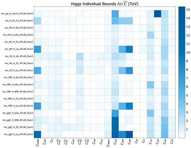

0.3.5 Global sensitivity from dataset variations (SMEFiT)
Finally, we should mention that ultimately the cleanest method to quantify the impact of a specific dataset or group of processes is to repeat the fit by removing them and studying what are the differences at the level of EFT coefficients.111One can also deploy the methods of Bayesian reweighting [97] to achieve the same goal. In this Section, we illustrate the method with results of the SMEFiT global fit reported in Ref. [32] without producing new results or recommending any EFT analysis. For example, Fig. 17 shows a comparison of the size of the 95% CL bounds on the Wilson coefficients considered in this analysis obtained in the global fit with those of fits to restricted datasets: a top-only, a Higgs-only, and a no-diboson fit. This way one can identify which coefficients are most sensitive to which datasets or groups of processes. Some observations that can be derived from these plots are that diboson data provides the unique handle on ; that Higgs processes provide some sensitivity on the top electroweak couplings and but much less than the top data itself; and that most of the purely bosonic operators are completely unconstrained unless Higgs measurements are included in the analysis.
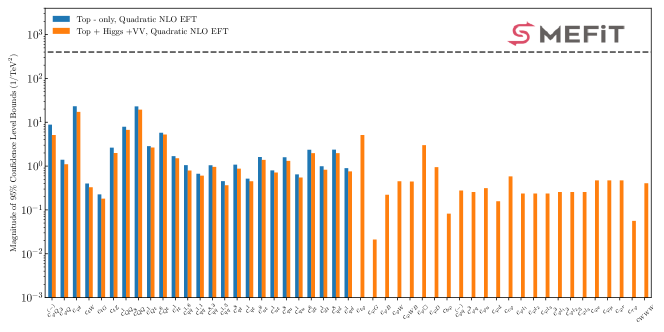
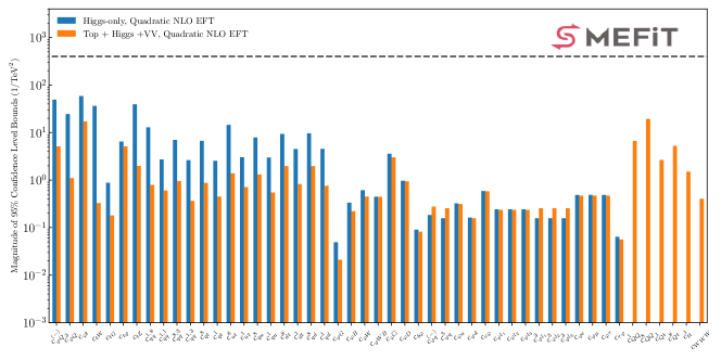
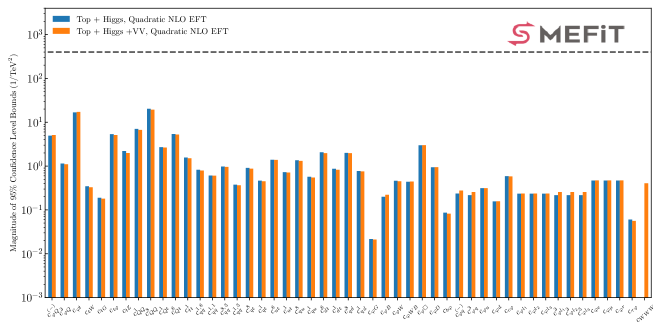
0.4 Summary
This note serves as a guide to experimental measurements and observables leading to EFT fits, but does not establish authoritative guidelines how those measurements should be performed. There is a spectrum of approaches to experimental measurements and observables, each approach has its own stronger and weaker sides, and none of the approaches has been established as the universally best approach to perform the EFT measurements. Analysis of LHC data in the framework of global EFT approach is a relative young field at this point. It has evolved from the less demanding task of interpreting of LHC data in the framework of standard model and of testing for its deviations in individual measurements. The field is still actively evolving, and the numbers of parameters and channels to be analyzed in an optimal and unbiased way are enormous. This poses both technical and conceptual challenges in performing the measurements, which will be resolved only gradually in close collaboration of experimental and theoretical particle physicists. One of the goals of ongoing effort is bridging the gap between theory and experimental communities working on EFT, and in particular concerning optimised analyses that so far are only accessible within the experiment.
The types of observables range from the usual quantities calculated for the SM measurements, to the EFT-sensitive observables, and to the optimized observables utilizing advanced matrix-element and machine-learning techniques. Good sensitivity to EFT effects is desired when constructing an observable. The single-step measurement approach allows extraction of EFT parameters from the data directly without intermediate results. This approach is conceptually straightforward, unbiased, can be an optimal approach, but suffers from complexity and the lack of re-interpretation capability. The two-step measurement approach allows wide dissemination and preservation of the data in the form of differential truth-level distribution (first step) for later re-interpretation (second step), but potentially this may lead to a non-optimal and/or biased analysis if care is not taken to address these concerns. Reporting the measurement results may represent a challenge on its own, as reporting the full likelihood function would be the ideal outcome and would allow interpretation and combination with other results. However, treatment of parameters with weak constraints and of systematic uncertainties, which may be correlated with other measurements, may complicate this process. This note does not provide specific guidelines how these issues should be technically addressed, but points to their importance.
In the second part of the note, we presented the main aspects of the mapping between observables and operators
in the context of global SMEFT interpretations, in the specific cases of two global fit efforts.
The set of operators considered in different flavour assumptions has been presented as well as a discussion of the
set of measurements which have been used to constrain these operators. The sensitivity of different observables
to different operators in the flavour universal scenario is quantified by examining the linear dependencies of Higgs,
diboson, and electroweak measurements obtained in the fitmaker analysis.
This allows the results of individual or marginalised constraints from global fits to be understood more intuitively.
Similarly, a detailed analysis based on the Fisher information formalism can be used to explore the relative sensitivity
of various observables to the EFT operators as presented in the SMEFiT analysis.
In the results of a global fit, the question also naturally arises as to which measurement is responsible for setting
the strongest constraints. In this note this decomposition is shown for individual constraints.
It has been observed that in order to understand the relation between operators and measurements,
a single tool is often not sufficient, and that the whole picture only comes together by comparing the output
of complementary tools. For example, the Fisher information is powerful, but in some cases only a direct fit
with some specific datasets omitted provides the necessary insight.
Finally results of the global fit have been shown.
Acknowledgments: This work was done on behalf of the LHC EFT WG and we would like to thank members of the LHC EFT WG for stimulating discussion of experimental measurements and observables which led to this document.
References
- [1] “LHC EFT Working Group.” https://lpcc.web.cern.ch/lhc-eft-wg.
- [2] S. Frixione, P. Nason and C. Oleari, Matching NLO QCD computations with parton shower simulations: the POWHEG method, JHEP 11 (2007) 070, [0709.2092].
- [3] J. Alwall, R. Frederix, S. Frixione, V. Hirschi, F. Maltoni et al., The automated computation of tree-level and next-to-leading order differential cross sections, and their matching to parton shower simulations, JHEP 1407 (2014) 079, [1405.0301].
- [4] T. Sjöstrand, S. Ask, J. R. Christiansen, R. Corke, N. Desai, P. Ilten et al., An introduction to PYTHIA 8.2, Comput. Phys. Commun. 191 (2015) 159, [1410.3012].
- [5] GEANT4 collaboration, S. Agostinelli et al., GEANT4–a simulation toolkit, Nucl. Instrum. Meth. A 506 (2003) 250–303.
- [6] T. Plehn, D. L. Rainwater and D. Zeppenfeld, Determining the Structure of Higgs Couplings at the LHC, Phys. Rev. Lett. 88 (2002) 051801, [hep-ph/0105325].
- [7] A. V. Gritsan, J. Roskes, U. Sarica, M. Schulze, M. Xiao and Y. Zhou, New features in the JHU generator framework: constraining Higgs boson properties from on-shell and off-shell production, Phys. Rev. D 102 (2020) 056022, [2002.09888].
- [8] D. Atwood and A. Soni, Analysis for magnetic moment and electric dipole moment form-factors of the top quark via e+ e- — t anti-t, Phys. Rev. D 45 (1992) 2405–2413.
- [9] M. Diehl and O. Nachtmann, Optimal observables for the measurement of three gauge boson couplings in e+ e- — W+ W-, Z. Phys. C 62 (1994) 397–412.
- [10] J. Neyman and E. S. Pearson, On the Problem of the Most Efficient Tests of Statistical Hypotheses, Phil. Trans. Roy. Soc. Lond. A 231 (1933) 289–337.
- [11] I. Anderson et al., Constraining Anomalous HVV Interactions at Proton and Lepton Colliders, Phys. Rev. D 89 (2014) 035007, [1309.4819].
- [12] G. D’Agostini, A Multidimensional unfolding method based on Bayes’ theorem, Nucl. Instrum. Meth. A 362 (1995) 487–498.
- [13] A. Hocker and V. Kartvelishvili, SVD approach to data unfolding, Nucl. Instrum. Meth. A 372 (1996) 469–481, [hep-ph/9509307].
- [14] “LHC Higgs Working Group.” https://twiki.cern.ch/twiki/bin/view/LHCPhysics/LHCHWG.
- [15] LHC Higgs Cross Section Working Group collaboration, D. de Florian et al., Handbook of LHC Higgs Cross Sections: 4. Deciphering the Nature of the Higgs Sector, 1610.07922.
- [16] J. Alwall et al., A standard format for Les Houches Event Files, Comput. Phys. Commun. 176 (2007) 300–304, [hep-ph/0609017].
- [17] CMS collaboration, A. M. Sirunyan et al., Constraints on anomalous Higgs boson couplings to vector bosons and fermions in its production and decay using the four-lepton final state, Phys. Rev. D 104 (2021) 052004, [2104.12152].
- [18] K. Kondo, Dynamical Likelihood Method for Reconstruction of Events With Missing Momentum. 1: Method and Toy Models, J. Phys. Soc. Jap. 57 (1988) 4126–4140.
- [19] P. J. Diggle and R. J. Gratton, Monte Carlo Methods of Inference for Implicit Statistical Models, in Journal of the Royal Statistical Society: Series B (Methodological), vol. 46, pp. 193–212, 1984. DOI.
- [20] K. Cranmer, J. Brehmer and G. Louppe, The frontier of simulation-based inference, Proc. Nat. Acad. Sci. 117 (2020) 30055–30062, [1911.01429].
- [21] J. Brehmer, K. Cranmer, G. Louppe and J. Pavez, Constraining Effective Field Theories with Machine Learning, Phys. Rev. Lett. 121 (2018) 111801, [1805.00013].
- [22] K. Cranmer, J. Pavez and G. Louppe, Approximating Likelihood Ratios with Calibrated Discriminative Classifiers, 1506.02169.
- [23] P. Baldi, K. Cranmer, T. Faucett, P. Sadowski and D. Whiteson, Parameterized neural networks for high-energy physics, Eur. Phys. J. C 76 (2016) 235, [1601.07913].
- [24] J. Brehmer, K. Cranmer, G. Louppe and J. Pavez, A Guide to Constraining Effective Field Theories with Machine Learning, Phys. Rev. D98 (2018) 052004, [1805.00020].
- [25] G. Aad and Others, “A morphing technique for signal modelling in a multidimensional space of coupling parameters.” 2015.
- [26] S. Chen, A. Glioti, G. Panico and A. Wulzer, Parametrized classifiers for optimal EFT sensitivity, JHEP 05 (2021) 247, [2007.10356].
- [27] J. Brehmer, G. Louppe, J. Pavez and K. Cranmer, Mining gold from implicit models to improve likelihood-free inference, 1805.12244.
- [28] M. Stoye, J. Brehmer, G. Louppe, J. Pavez and K. Cranmer, Likelihood-free inference with an improved cross-entropy estimator, 1808.00973.
- [29] J. Brehmer, F. Kling, I. Espejo and K. Cranmer, MadMiner: Machine Learning-Based Inference for Particle Physics, Computing and Software for Big Science 4 (2020) , [1907.10621].
- [30] J. Brehmer, F. Kling, I. Espejo, S. Perez and K. Cranmer, Madminer, Nov., 2021. If you use this software, please cite it as below., 10.5281/zenodo.5654822.
- [31] J. Ellis, M. Madigan, K. Mimasu, V. Sanz and T. You, Top, Higgs, Diboson and Electroweak Fit to the Standard Model Effective Field Theory, 2012.02779.
- [32] J. J. Ethier, G. Magni, F. Maltoni, L. Mantani, E. R. Nocera, J. Rojo et al., Combined SMEFT interpretation of Higgs, diboson, and top quark data from the LHC, 2105.00006.
- [33] B. Grzadkowski, M. Iskrzynski, M. Misiak and J. Rosiek, Dimension-Six Terms in the Standard Model Lagrangian, JHEP 10 (2010) 085, [1008.4884].
- [34] N. P. Hartland, F. Maltoni, E. R. Nocera, J. Rojo, E. Slade, E. Vryonidou et al., A Monte Carlo global analysis of the Standard Model Effective Field Theory: the top quark sector, JHEP 04 (2019) 100, [1901.05965].
- [35] D. Barducci et al., Interpreting top-quark LHC measurements in the standard-model effective field theory, 1802.07237.
- [36] G. D’Ambrosio, G. F. Giudice, G. Isidori and A. Strumia, Minimal flavor violation: An Effective field theory approach, Nucl. Phys. B645 (2002) 155–187, [hep-ph/0207036].
- [37] C. Degrande, G. Durieux, F. Maltoni, K. Mimasu, E. Vryonidou and C. Zhang, Automated one-loop computations in the SMEFT, 2008.11743.
- [38] J. J. Ethier, R. Gomez-Ambrosio, G. Magni and J. Rojo, SMEFT analysis of vector boson scattering and diboson data from the LHC Run II, Eur. Phys. J. C 81 (2021) 560, [2101.03180].
- [39] ATLAS collaboration, G. Aad et al., Measurements of top-quark pair differential cross-sections in the lepton+jets channel in collisions at TeV using the ATLAS detector, Eur. Phys. J. C76 (2016) 538, [1511.04716].
- [40] CMS collaboration, V. Khachatryan et al., Measurement of the differential cross section for top quark pair production in pp collisions at , Eur. Phys. J. C75 (2015) 542, [1505.04480].
- [41] CMS collaboration, A. M. Sirunyan et al., Measurement of double-differential cross sections for top quark pair production in pp collisions at TeV and impact on parton distribution functions, Eur. Phys. J. C77 (2017) 459, [1703.01630].
- [42] ATLAS collaboration, M. Aaboud et al., Measurement of the W boson polarisation in events from pp collisions at = 8 TeV in the lepton + jets channel with ATLAS, Eur. Phys. J. C77 (2017) 264, [1612.02577].
- [43] CMS collaboration, V. Khachatryan et al., Measurement of the W boson helicity fractions in the decays of top quark pairs to lepton jets final states produced in pp collisions at 8TeV, Phys. Lett. B762 (2016) 512–534, [1605.09047].
- [44] CMS collaboration, V. Khachatryan et al., Measurement of differential cross sections for top quark pair production using the lepton+jets final state in proton-proton collisions at 13 TeV, Phys. Rev. D95 (2017) 092001, [1610.04191].
- [45] CMS collaboration, A. M. Sirunyan et al., Measurement of differential cross sections for the production of top quark pairs and of additional jets in lepton+jets events from pp collisions at 13 TeV, Phys. Rev. D97 (2018) 112003, [1803.08856].
- [46] CMS collaboration, A. M. Sirunyan et al., Measurement of normalized differential cross sections in the dilepton channel from pp collisions at TeV, JHEP 04 (2018) 060, [1708.07638].
- [47] ATLAS collaboration, M. Aaboud et al., Measurement of top quark pair differential cross-sections in the dilepton channel in collisions at = 7 and 8 TeV with ATLAS, Phys. Rev. D 94 (2016) 092003, [1607.07281].
- [48] ATLAS collaboration, G. Aad et al., Measurements of top-quark pair differential and double-differential cross-sections in the +jets channel with collisions at TeV using the ATLAS detector, Eur. Phys. J. C 79 (2019) 1028, [1908.07305].
- [49] CMS collaboration, A. M. Sirunyan et al., Measurements of differential cross sections in proton-proton collisions at 13 TeV using events containing two leptons, JHEP 02 (2019) 149, [1811.06625].
- [50] ATLAS, CMS collaboration, M. Aaboud et al., Combination of inclusive and differential charge asymmetry measurements using ATLAS and CMS data at and 8 TeV, JHEP 04 (2018) 033, [1709.05327].
- [51] ATLAS collaboration, Inclusive and differential measurement of the charge asymmetry in events at 13 TeV with the ATLAS detector, .
- [52] CMS collaboration, A. M. Sirunyan et al., Measurements of cross sections in association with jets and inclusive jets and their ratio using dilepton final states in pp collisions at = 13 TeV, Phys. Lett. B776 (2018) 355–378, [1705.10141].
- [53] CMS collaboration, A. M. Sirunyan et al., Search for standard model production of four top quarks with same-sign and multilepton final states in proton–proton collisions at , Eur. Phys. J. C78 (2018) 140, [1710.10614].
- [54] CMS collaboration, A. M. Sirunyan et al., Search for production of four top quarks in final states with same-sign or multiple leptons in proton-proton collisions at 13 TeV, Eur. Phys. J. C 80 (2020) 75, [1908.06463].
- [55] ATLAS collaboration, G. Aad et al., Evidence for production in the multilepton final state in proton–proton collisions at TeV with the ATLAS detector, Eur. Phys. J. C 80 (2020) 1085, [2007.14858].
- [56] ATLAS collaboration, M. Aaboud et al., Measurements of inclusive and differential fiducial cross-sections of production with additional heavy-flavour jets in proton-proton collisions at = 13 TeV with the ATLAS detector, JHEP 04 (2019) 046, [1811.12113].
- [57] CMS collaboration, A. M. Sirunyan et al., Measurement of the production cross section in the all-jet final state in pp collisions at 13 TeV, Phys. Lett. B 803 (2020) 135285, [1909.05306].
- [58] CMS collaboration, V. Khachatryan et al., Observation of top quark pairs produced in association with a vector boson in pp collisions at TeV, JHEP 01 (2016) 096, [1510.01131].
- [59] CMS collaboration, A. M. Sirunyan et al., Measurement of the cross section for top quark pair production in association with a W or Z boson in proton-proton collisions at 13 TeV, JHEP 08 (2018) 011, [1711.02547].
- [60] ATLAS collaboration, G. Aad et al., Measurement of the and production cross sections in pp collisions at TeV with the ATLAS detector, JHEP 11 (2015) 172, [1509.05276].
- [61] ATLAS collaboration, M. Aaboud et al., Measurement of the and production cross sections in multilepton final states using 3.2 fb-1 of collisions at = 13 TeV with the ATLAS detector, Eur. Phys. J. C77 (2017) 40, [1609.01599].
- [62] ATLAS collaboration, M. Aaboud et al., Measurement of the and cross sections in proton-proton collisions at TeV with the ATLAS detector, Phys. Rev. D 99 (2019) 072009, [1901.03584].
- [63] CMS collaboration, A. M. Sirunyan et al., Measurement of top quark pair production in association with a Z boson in proton-proton collisions at 13 TeV, JHEP 03 (2020) 056, [1907.11270].
- [64] CMS collaboration, V. Khachatryan et al., Measurement of the t-channel single-top-quark production cross section and of the CKM matrix element in pp collisions at = 8 TeV, JHEP 06 (2014) 090, [1403.7366].
- [65] CMS Collaboration collaboration, A. M. Sirunyan et al., Single top t-channel differential cross section at 8 TeV, CMS-PAS-TOP-14-004 (2014) https://cds.cern.ch/record/1956681.
- [66] ATLAS collaboration, M. Aaboud et al., Fiducial, total and differential cross-section measurements of -channel single top-quark production in collisions at 8 TeV using data collected by the ATLAS detector, Eur. Phys. J. C77 (2017) 531, [1702.02859].
- [67] ATLAS collaboration, G. Aad et al., Evidence for single top-quark production in the -channel in proton-proton collisions at 8 TeV with the ATLAS detector using the Matrix Element Method, Phys. Lett. B756 (2016) 228–246, [1511.05980].
- [68] CMS collaboration, V. Khachatryan et al., Search for s channel single top quark production in pp collisions at and 8 TeV, JHEP 09 (2016) 027, [1603.02555].
- [69] ATLAS collaboration, M. Aaboud et al., Measurement of the inclusive cross-sections of single top-quark and top-antiquark -channel production in collisions at = 13 TeV with the ATLAS detector, JHEP 04 (2017) 086, [1609.03920].
- [70] CMS collaboration, V. Khachatryan et al., Measurement of the differential cross section for -channel single-top-quark production at , CMS-PAS-TOP-16-004 (2016) https://cds.cern.ch/record/2151074.
- [71] CMS collaboration, A. M. Sirunyan et al., Cross section measurement of -channel single top quark production in pp collisions at 13 TeV, Phys. Lett. B772 (2017) 752–776, [1610.00678].
- [72] CMS collaboration, A. M. Sirunyan et al., Measurement of differential cross sections and charge ratios for t-channel single top quark production in proton–proton collisions at , Eur. Phys. J. C 80 (2020) 370, [1907.08330].
- [73] ATLAS collaboration, G. Aad et al., Measurement of the production cross-section of a single top quark in association with a boson at 8 TeV with the ATLAS experiment, JHEP 01 (2016) 064, [1510.03752].
- [74] CMS collaboration, S. Chatrchyan et al., Observation of the associated production of a single top quark and a boson in collisions at 8 TeV, Phys. Rev. Lett. 112 (2014) 231802, [1401.2942].
- [75] ATLAS collaboration, M. Aaboud et al., Measurement of the cross-section for producing a W boson in association with a single top quark in pp collisions at TeV with ATLAS, JHEP 01 (2018) 063, [1612.07231].
- [76] CMS collaboration, A. M. Sirunyan et al., Measurement of the production cross section for single top quarks in association with W bosons in proton-proton collisions at 13 TeV, JHEP (2018) , [1805.07399].
- [77] CMS collaboration, A. M. Sirunyan et al., Measurement of the associated production of a single top quark and a Z boson in pp collisions at TeV, Phys. Lett. B779 (2018) 358–384, [1712.02825].
- [78] ATLAS collaboration, M. Aaboud et al., Measurement of the production cross-section of a single top quark in association with a Z boson in proton–proton collisions at 13 TeV with the ATLAS detector, Phys. Lett. B780 (2018) 557–577, [1710.03659].
- [79] ATLAS collaboration, G. Aad et al., Measurement of single top-quark production in association with a boson in the single-lepton channel at TeV with the ATLAS detector, 2007.01554.
- [80] ATLAS collaboration, G. Aad et al., Observation of the associated production of a top quark and a boson in collisions at TeV with the ATLAS detector, JHEP 07 (2020) 124, [2002.07546].
- [81] CMS collaboration, A. M. Sirunyan et al., Observation of Single Top Quark Production in Association with a Boson in Proton-Proton Collisions at =13 TeV, Phys. Rev. Lett. 122 (2019) 132003, [1812.05900].
- [82] ATLAS, CMS collaboration, G. Aad et al., Measurements of the Higgs boson production and decay rates and constraints on its couplings from a combined ATLAS and CMS analysis of the LHC pp collision data at and 8 TeV, JHEP 08 (2016) 045, [1606.02266].
- [83] ATLAS collaboration, G. Aad et al., Combined measurements of Higgs boson production and decay using up to fb-1 of proton-proton collision data at 13 TeV collected with the ATLAS experiment, Phys. Rev. D 101 (2020) 012002, [1909.02845].
- [84] CMS collaboration, A. M. Sirunyan et al., Combined measurements of Higgs boson couplings in proton–proton collisions at , Eur. Phys. J. C 79 (2019) 421, [1809.10733].
- [85] ATLAS collaboration, M. Aaboud et al., Combined measurement of differential and total cross sections in the and the decay channels at TeV with the ATLAS detector, Phys. Lett. B 786 (2018) 114–133, [1805.10197].
- [86] CMS collaboration, A. M. Sirunyan et al., Measurement and interpretation of differential cross sections for Higgs boson production at 13 TeV, Phys. Lett. B 792 (2019) 369–396, [1812.06504].
- [87] ATLAS collaboration, M. Aaboud et al., Measurement of VH, production as a function of the vector-boson transverse momentum in 13 TeV pp collisions with the ATLAS detector, JHEP 05 (2019) 141, [1903.04618].
- [88] CMS collaboration, Measurements of Higgs boson production via gluon fusion and vector boson fusion in the diphoton decay channel at TeV, .
- [89] ALEPH, DELPHI, L3, OPAL, LEP Electroweak collaboration, S. Schael et al., Electroweak Measurements in Electron-Positron Collisions at W-Boson-Pair Energies at LEP, Phys. Rept. 532 (2013) 119–244, [1302.3415].
- [90] ATLAS Collaboration collaboration, Measurement of production cross sections and gauge boson polarisation in collisions at TeV with the ATLAS detector, CERN, Geneva, ATLAS-CONF-2018-034, Jul, 2018.
- [91] CMS collaboration, A. M. Sirunyan et al., Measurements of the pp WZ inclusive and differential production cross section and constraints on charged anomalous triple gauge couplings at 13 TeV, JHEP 04 (2019) 122, [1901.03428].
- [92] ATLAS collaboration, M. Aaboud et al., Measurement of fiducial and differential production cross-sections at TeV with the ATLAS detector, Eur. Phys. J. C 79 (2019) 884, [1905.04242].
- [93] E. Bagnaschi, J. Ellis, M. Madigan, K. Mimasu, V. Sanz and T. You, SMEFT analysis of mW, JHEP 08 (2022) 308, [2204.05260].
- [94] ATLAS collaboration, G. Aad et al., Higgs boson production cross-section measurements and their EFT interpretation in the decay channel at 13 TeV with the ATLAS detector, Eur. Phys. J. C 80 (2020) 957, [2004.03447].
- [95] A. Falkowski and F. Riva, Model-independent precision constraints on dimension-6 operators, JHEP 02 (2015) 039, [1411.0669].
- [96] J. Brehmer, F. Kling, T. Plehn and T. M. P. Tait, Better Higgs-CP Tests Through Information Geometry, Phys. Rev. D97 (2018) 095017, [1712.02350].
- [97] S. van Beek, E. R. Nocera, J. Rojo and E. Slade, Constraining the SMEFT with Bayesian reweighting, SciPost Phys. 7 (2019) 070, [1906.05296].