QMUL-PH-18-18

Effective Field Theory in the top sector: do multijets help?

Christoph Englert^a, Michael Russell^b  and Chris D. White^c

^a SUPA, School of Physics and Astronomy, University of Glasgow,

Glasgow, G12 8QQ, United Kingdom

^b Institut für Theoretische Physik, Universität Heidelberg, Germany
^c Centre for Research in String Theory, School of Physics and Astronomy,

Queen Mary University of London, 327 Mile End Road,

London E1 4NS, United Kingdom

Many studies of possible new physics employ effective field theory (EFT), whereby corrections to the Standard Model take the form of higher-dimensional operators, suppressed by a large energy scale. Fits of such a theory to data typically use parton level observables, which limits the datasets one can use. In order to theoretically model search channels involving many additional jets, it is important to include tree-level matrix elements matched to a parton shower algorithm, and a suitable matching procedure to remove the double counting of additional radiation. There are then two potential problems: (i) EFT corrections are absent in the shower, leading to an extra source of discontinuities in the matching procedure; (ii) the uncertainty in the matching procedure may be such that no additional constraints are obtained from observables sensitive to radiation. In this paper, we review why the first of these is not a problem in practice, and perform a detailed study of the second. In particular, we quantify the additional constraints on EFT expected from top pair plus multijet events, relative to inclusive top pair production alone.

1 Introduction

The search for physics beyond the Standard Model (BSM) is the most pressing problem in particle physics, especially given the on-going experimental programme at the Large Hadron Collider. To date, clear signatures of BSM physics have remained elusive, although it is widely suspected that the new physics may have something to do with the nature of electroweak symmetry breaking, and thus affect the behaviour of the recently discovered Higgs boson or, due to its large Yukawa coupling with the former, the top quark.

The lack of clear evidence for BSM physics thus far motivates the use of effective field theory [1, 2, 3, 4, 5, 6] (for a comprehensive review see [7]), in which one characterises corrections to the SM Lagrangian by gauge-invariant higher dimensional operators built from the SM fields. This has the advantage of being manifestly model independent, but is only applicable if the lowest energy scale associated with the new physics is above the typical energies probed by the collider of interest. Given that this is likely to be a viable situation at the LHC, such techniques have been widely used in the contexts of Higgs and electroweak precision physics [8, 9, 10, 11, 12, 13, 14, 15, 16, 17, 18, 19, 20, 21, 22, 23, 24, 25, 26, 27, 28, 29, 30, 31, 32, 33, 34, 35, 36, 37, 38, 39, 40, 41, 42, 43, 44, 45, 46, 47, 48, 49, 50, 51, 52, 53, 54, 55, 56]. A priori, it is not clear whether new physics will first show up in the behaviour of the Higgs boson rather than the top quark. Thus, a number of more recent studies have looked at constraining effective theory in the top quark sector [57, 58, 59, 60, 61, 62, 63, 64, 65, 66] (see also [67, 68, 69, 70, 71, 72, 73, 74, 75, 76, 77, 78, 79, 80, 81, 82] for analyses using the alternative language of anomalous couplings).

Ideally, one should attempt to constrain all possible higher dimensional operators, using all possible experimental data. To this end, Refs. [83, 84] have presented a proof of principle that such global fits are possible (see also Refs. [85, 86, 87, 49, 88, 89, 90, 91, 65, 66] for related work in both the top and Higgs sectors). In particular, the fit of Ref. [84] directly constrained the coefficients of all (combinations of) operators affecting single and double top production and decay, as well as associated production of a vector boson, using a wide variety of datasets from the Tevatron and LHC (runs I and II). These datasets were all corrected back to parton level, and compared with tree-level theory results, supplemented with NLO information using (bin-by-bin) K-factors. There are many available datasets, however, which do not admit such a simple theoretical description. A typical example is observables sensitive to multiple final state jets of QCD radiation, which cannot be accurately modelled by available LO or NLO matrix elements. To this end, one may employ parton shower algorithms to simulate additional radiation, and many general purpose codes are available. Furthermore, parton showers may be systematically matched to matrix elements calculated at next-to-leading order in QCD perturbation theory [92, 93, 94, 95, 96, 97, 98, 99], and to algorithms which model the hadronisation of final state quarks and gluons. Computations of this type for top-related processes, including higher dimensional operators, have been recently presented in Refs. [66, 39].

When many final state jets are required in a given observable, one must systematically improve the output of a parton shower by including higher order tree-level matrix elements. A matching prescription is then needed to avoid double counting of radiation included in both the matrix elements and the shower, and different schemes have been presented in Refs. [100, 101, 102, 103, 104, 105]. The aim of such a matching procedure, roughly speaking, is to ensure that jets that are widely separated from others in a given event are generated by the hard matrix elements, and those which are approximately collinear with other jets are generated by the parton shower. The separation between these two regimes is specified by a matching scale $Q$, and this must be carefully chosen so as to avoid discontinuities in distributions relating to additional jet radiation: too small, and matrix elements will be evaluated in momentum regions in which they are becoming collinearly singular; too large, and the parton shower will be used in kinematic regions where it fails to approximate higher order matrix elements sufficiently accurately. Such discontinuities thus represent a mismatch between how QCD radiation is described by a parton shower, and by exact matrix elements, and is a problem even within the SM alone.

When higher dimensional operators are added to the SM, a second source of discontinuity arises. The operators generate additional Feynman rules, including couplings to quarks and gluons. Thus, rates for the emission of QCD radiation become modified. If matrix elements in this theory are matched to a parton shower, it follows that widely separated jets (generated by the matrix elements) will include the effect of the BSM physics, whereas those which are not widely separated will be generated by a parton shower which contains SM radiation only, leading to a mismatch between the two descriptions. Naïvely, one may expect this effect to be small: first of all, the higher dimensional operators are typically suppressed by a large energy scale. Moreover, they contain momentum-dependent numerators that tend to boost radiated particles to higher transverse momenta, thus widely separated from other particles. However, there is a more formal argument one can give to explain why any additional discontinuity resulting from the lack of EFT operators in the shower is negligible relative to the SM effect, related to the fact that emissions from EFT operators do not give rise to infrared singularities. Although the ideas involved are well-known to a QCD audience, this argument is not well-known in the BSM literature, and thus we provide a detailed explanation in this paper.

Armed with results for matrix elements containing EFT corrections matched to a parton shower one may address, for a particular production process / observable requiring such a theory description, whether or not useful additional constraints on given operators can be obtained. Our motivation here is extending the global EFT fits of Refs. [83, 84] to include particle-level observables, for which a notable example is top quark pair production in association with multiple jets. For this process to provide a worthwhile new input to a global EFT fit, it is important to check that useful additional constraints are obtained by including radiation observables as well as those related to the top particles alone . We will study this in detail for a number of operators, whose coefficients are set to values consistent with recent constraints, finding that indeed there is more information to be gleaned by adding observables sensitive to extra radiation.

The structure of the paper is as follows. In section 2, we examine the role of effective theory corrections to the three-gluon vertex, and argue that any additional discontinuity when matching matrix elements and parton showers is kinematically subleading to the existing SM discontinuity. In section 3, we study a number of observables in top plus multijet production, and examine in detail whether additional constraints can be obtained by using observables sensitive to additional jet radiation, given the matching uncertainties. Finally, we conclude in section 4.

2 Matching effective theory matrix elements with parton showers

As discussed above, if one matches higher order tree-level matrix elements containing higher dimensional operators to a parton shower, BSM effects are included in the matrix elements, but not the shower. Information about the BSM physics is then missing in additional jets that are generated by the shower, rather than the matrix elements, where the former are formally correct only in the collinear limit. This in turn means that jets which are sufficiently collinear to other jets (defined in terms of the matching scale) in a given event are potentially missing BSM effects. In this section, we review in detail why this is not actually a problem in practice, due to the differing nature of SM and BSM radiation in the collinear limit. Our presentation will be similar to that of Refs. [106, 107]. For illustrative purposes, we consider the case of a gluon which branches into a gluon pair, with momenta labelled as in Fig. 1.

Figure 1: A gluon emerges from a scattering amplitude, before branching into two gluons, with angular separation $\theta$.

The intermediate momentum $p_{a}=p_{b}+p_{c}$ has virtuality

$$t\equiv p_{a}^{2}\simeq z(1-z)E_{a}^{2}\theta^{2},$$ (2.1)

where

$$z=\frac{E_{b}}{E_{a}}=1-\frac{E_{c}}{E_{a}}$$ (2.2)

is the fraction of the energy of parton $a$ that is carried by parton $b$. Given that this virtuality is small as $\theta\rightarrow 0$, we may treat parton $a$ as being approximately on-shell in the collinear limit. We can then consider the amplitude for emission of a gluon from the leg $p_{a}$, which will be given by

$${\cal M}^{a_{2},a_{3},\ldots}_{n+1}(p_{b},p_{c},\ldots)=\epsilon^{\mu_{1}}(p_{a})\,\epsilon^{\mu_{2}}(p_{b})\,\epsilon^{\mu_{3}}(p_{c})V^{a_{1}a_{2}a_{3}}_{\mu_{1}\mu_{2}\mu_{3}}(p_{a},p_{b},p_{c}){\cal M}^{a_{1},\ldots}_{n}(p_{a},\ldots),$$ (2.3)

where ${\cal M}_{n}$ is the amplitude before the gluon branching, $\{a_{i}\}$ are adjoint indices of the gluons, and the ellipses denote all momenta and colour degrees of freedom associated with partons that are suppressed in Fig. 1. Furthermore, $\epsilon^{\mu_{i}}$ is the polarisation vector of parton $i$, and $V^{a_{1}a_{2}a_{3}}_{\mu_{1}\mu_{2}\mu_{3}}$ the three-gluon vertex. We may write the latter as

$$V^{a_{1}a_{2}a_{3}}_{\mu_{1}\mu_{2}\mu_{3}}(p_{1},p_{2},p_{3})=V^{a_{1}a_{2}a_{3}}_{{\rm SM},\mu_{1}\mu_{2}\mu_{3}}(p_{1},p_{2},p_{3})+V^{a_{1}a_{2}a_{3}}_{{\rm BSM},\mu_{1}\mu_{2}\mu_{3}}(p_{1},p_{2},p_{3}),$$ (2.4)

where the first term on the right-hand side is the Standard Model component (coming purely from the QCD Lagrangian), and the second term collects the additional contributions arising from higher dimensional operators. To this end let us consider the following three-gluon operator:

$${\cal O}_{G}=f_{a_{1}a_{2}a_{3}}\,G_{\mu}^{a_{1}\nu}\,G_{\nu}^{a_{2}\lambda}\,G_{\lambda}^{a_{3}\mu},$$ (2.5)

where $G^{A}_{\mu\nu}$ is the gluon field strength tensor. We may also consider the associated Lagrangian

$${\cal L}_{G}=\frac{C_{G}}{\Lambda^{2}}\frac{1}{3!}{\cal O}_{G},$$ (2.6)

where $\Lambda$ is the new physics scale, and $C_{G}$ an unknown coefficient. The effect of this Lagrangian is to generate new interactions involving the gluon field, and in particular to modify the Feynman rule for the three-gluon vertex. Explicit results for the two terms on the right-hand side of Eq. (2.4) are then

$$V^{a_{1}a_{2}a_{3}}_{{\rm SM},\mu_{1}\mu_{2}\mu_{3}}(p_{1},p_{2},p_{3})=g_{s}f_{a_{1}a_{2}a_{3}}\left[(p_{1}-p_{2})_{\mu_{3}}\eta_{\mu_{1}\mu_{2}}+(p_{3}-p_{1})_{\mu_{2}}\eta_{\mu_{1}\mu_{3}}+(p_{2}-p_{3})_{\mu_{1}}\eta_{\mu_{2}\mu_{3}}\right]$$ (2.7)

and

$$V^{a_{1}a_{2}a_{3}}_{{\rm BSM},\mu_{1}\mu_{2}\mu_{3}}(p_{1},p_{2},p_{3})=\frac{C_{G}}{\Lambda^{2}}f^{a_{1}a_{2}a_{3}}\Big{[}p_{1\mu_{2}}\,p_{2\mu_{3}}\,p_{3\mu_{1}}-p_{1\mu_{3}}\,p_{2\mu_{1}}\,p_{3\mu_{2}}$$

$$\quad+(p_{1}\cdot p_{2})p_{3[\mu_{2}}\,\eta_{\mu_{1}]\mu_{3}}+(p_{1}\cdot p_{3})p_{2[\mu_{1}}\,\eta_{\mu_{3}]\mu_{2}}+(p_{2}\cdot p_{3})p_{1[\mu_{3}}\,\eta_{\mu_{2}]\mu_{1}}\Big{]},$$ (2.8)

where the square brackets in the subscripts denote antisymmetrisation of indices.

In constructing the squared amplitude in the SM, one need only include diagrams in which the radiated gluon $p_{b}$ lands on the leg $p_{a}$ on both sides of the final state cut. From Eq. (2.3), the sum of all such diagrams, summed over all final state polarisations and averaged over the polarisation of the branching parton $p_{a}$, is (in four spacetime dimensions)

$$\overline{|{\cal M}^{a_{2},a_{3},\ldots}_{n+1}(p_{b},p_{c},\ldots)|^{2}}=\frac{1}{2}|{\cal M}^{a_{1},\ldots}_{n}(p_{a},\ldots)|^{2}\sum_{\rm pols}\Big{[}\epsilon^{\mu_{1}}(p_{a})\,\epsilon^{\mu_{2}}(p_{b})\,\epsilon^{\mu_{3}}(p_{c})V^{a_{1}a_{2}a_{3}}_{\mu_{1}\mu_{2}\mu_{3}}(p_{a},p_{b},p_{c})\Big{]}^{2}.$$ (2.9)

In order to evaluate this expression, one may choose an explicit basis of polarisation vectors for each parton, $\epsilon(p_{i})\in\{\epsilon^{\rm in}_{i},\epsilon^{\rm out}_{i}\}$, pointing in and out of the scattering plane respectively. One may then use the dot products [106, 107]

$$\epsilon^{\rm in}_{i}\cdot\epsilon^{\rm in}_{j}=\epsilon^{\rm out}_{i}\cdot\epsilon^{\rm out}_{j}=-1,\quad\epsilon^{\rm in}_{i}\cdot\epsilon^{\rm out}_{j}=\epsilon^{\rm out}_{i}\cdot p_{j}=0,$$ (2.10)

as well as

$$\epsilon_{a}^{\rm in}\cdot p_{b}\simeq-z(1-z)E_{a}\theta,\quad\epsilon_{b}^{\rm in}\cdot p_{c}\simeq(1-z)E_{a}\theta,\quad\epsilon_{c}^{\rm in}\cdot p_{b}\simeq-zE_{a}\theta$$ (2.11)

and

$$p_{a}\cdot p_{b}=p_{a}\cdot p_{c}=-p_{b}\cdot p_{c}\simeq-\frac{z(1-z)E_{a}^{2}\theta^{2}}{2},$$ (2.12)

to obtain

$$\overline{|{\cal M}_{n+1}(p_{b},p_{c},\ldots)|^{2}} =\frac{4C_{A}g_{s}^{2}}{t}\left[\frac{1-z}{z}+\frac{z}{1-z}+z(1-z)\right.$$

$$\left.+\frac{C_{G}}{\Lambda^{2}}\frac{z(1-z)E_{a}^{2}\theta^{2}}{2}-\left(\frac{C_{G}}{\Lambda^{2}}\right)^{2}\frac{z^{3}(1-z)^{3}E_{a}^{4}\theta^{4}}{4}\right]|{\cal M}^{a_{1},\ldots}_{n}(p_{a},\ldots)|^{2}.$$ (2.13)

The terms in the first line are recognisable as the usual QCD splitting function $P_{gg}(z)$ describing the probability for a gluon to branch into two gluons. The first term in the second line arises from interference of the BSM contribution with the SM, and is suppressed by the inverse square of the new physics scale. The second term in the second line is quadratic in the new physics, and would mix with potential dimension eight effects in the effective theory expansion, thus is formally of higher order and can be neglected. It is only the interference term that constitutes those BSM corrections that are missing in the collinear region. However, upon studying this term, we see explicitly that it contains a factor of $\theta^{2}$ and, hence, is formally kinematically suppressed in the collinear limit. From Eq. (2.1), the prefactor in Eq. (2.13) is ${\cal O}(\theta^{-2})$, and thus the SM term contains the well-known collinear enhancement of QCD radiation. The BSM interference term (including the prefactor) is ${\cal O}(\theta^{0})$, and will be negligible provided that the matching scale between matrix elements and parton shower is chosen to be sufficiently small. Put another way, any additional source of discontinuity in jet-related distributions coming from the absence of BSM corrections in the shower, is kinematically suppressed relative to the discontinuity already present in the SM.

Given the above discussion, one may ponder whether it is possible to nevertheless include the BSM interference contribution in Eq. (2.13) in the gluon branching probability, despite the fact that this corresponds (eventually) to resumming a subleading contribution. However, such a procedure would be formally incorrect. In general, the radiated gluon may be emitted from parton leg $i$, and land on leg $j$ in the conjugate amplitude. Above, we have considered only contributions for which $i=j$, as shown in Fig. 2(a).

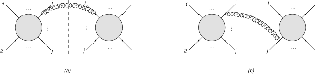
Figure 2: A gluon is emitted from parton leg $i$ and lands on leg $j$ in the conjugate amplitude: (a) the case $i=j$; (b) the case $i\neq j$.

This is correct for the SM: such contributions, as we have seen above, are ${\cal O}(\theta^{-2})$, whereas diagrams with $i=j$ (Fig. 2(b)) are ${\cal O}(\theta^{0})$. It is incomplete, however, for the BSM interference contributions. Diagrams with $i=j$ and $i\neq j$ are both of the same kinematic order (${\cal O}(\theta^{0})$). All of them must be therefore be included to ensure a gauge invariant result, so that it makes no sense to resum only a subset of them.

Above we have examined only the operator of Eq. (2.5). However, the kinematic suppression that we have observed will be fully general, including operators that affect other parton branchings, involving (anti-)quarks in addition to gluons. This follows from the fact that any dimension six operator appears in the Lagrangian with a dimensionless coefficient $C_{i}$, and an inverse power of the new physics scale, $\Lambda^{-2}$. For the Lagrangian to have the correct dimension, the momentum space Lagrangian must contain two powers of momentum, that combine with $\Lambda$ to make a dimensionless ratio. We can see this explicitly in the example of the three-gluon operator given above: the BSM vertex of Eq. (2.8) contains two additional powers of momentum relative to the SM result of Eq. (2.7). When evaluating the graph of Fig. 1, there is only one momentum scale available, namely the virtuality of the branching parton, $p_{a}^{2}$. Thus, the higher dimensional operator must contribute an interference term

$$\sim\frac{p_{a}^{2}}{\Lambda^{2}}\sim\frac{z(1-z)E_{a}^{2}\theta^{2}}{\Lambda^{2}},$$ (2.14)

where we have used Eq. (2.1). This is indeed observed in Eq. (2.13).

We have so far seen that the effects of higher dimensional operators are negligible in the collinear region, and thus should not significantly contribute to discontinuities in jet-related kinematic distributions when matching parton showers (based on enhanced collinear radiation) to matrix elements. However, this is not the full story. Parton shower algorithms also include the effects of wide-angle soft radiation, by e.g. explicit angular ordering, or the choice of evolution variable [106, 107]. The above dimensional argument applies also in this case: for soft, but not necessarily collinear, emissions, the only momentum scale that can combine with the new physics scale in the BSM vertex for the radiated parton is the virtuality of the emitting parton. This remains small if the emitted parton is soft. Indeed, looking at the interference term in Eq. (2.13), we see that this vanishes as $z\rightarrow 0$ or $z\rightarrow 1$, corresponding to the two limits in which either parton $a$ or parton $b$ is soft. There is thus no soft singularity from the BSM part, mirroring the lack of collinear singularity. Furthermore, the fact that the virtuality of the emitting parton is the only relevant scale that can combine with the new physics scale in the soft or collinear region means that the above discussion is fully general, and applies to all QCD dimension six operators.

In this section, we have reviewed in detail the fact that additional radiation produced by EFT operators is not associated with collinear singularities, and thus does not lead to SM-like discontinuities when matching tree-level matrix elements with a parton shower. However, in order to obtain meaningful constraints from observables requiring such a theory description, it is important to examine whether or not deviations due to EFT corrections lead to significant new information, in light of the theoretical uncertainties due to the matching procedure. This is the subject of the following section.

3 Results

As discussed above, the aim of our study is to ascertain whether or not jet observables in top production provide additional constraints on new physics (as described using EFT), relative to observables only involving the top quarks (for similar analyses of BSM QCD multi-jet production see [108]). To this end, we must first examine the matching uncertainty affecting how the jets are modelled.

3.1 Effect of dimension six operators on jet radiation

In this section, we present a number of example distributions, including EFT effects consistent with current constraints on operator coefficients [84]. Results are obtained as follows. We implement EFT operators in a FeynRules [109] model file, and interface this with MadGraph5_aMC@NLO [110] for the generation of tree-level events containing top pairs with up to 2 jets. These are matched to the parton shower Pythia 8 [111], using the default MadGraph MLM-based matching scheme [112], with a central matching scale $Q=30$ GeV. Our default choice for the renormalisation and factorisation scales is the top mass, $\mu_{\rm ren}=\mu_{\rm fact.}=m_{t}$, and we use the parton distributions of Ref. [113]. We cluster all visible final-state particles into jets using the anti-$k_{T}$ algorithm [114] with jet radius $R=0.4$, as implemented in FastJet [115]. We consider only the dilepton final state, and require both leptons to be isolated from hadronic activity, defined via the requirement that the total transverse momentum with a cone of radius $\Delta R=0.3$ around the lepton satisfies $p_{T}^{\rm cone}\leq 0.1\times p_{T,l}$, where $p_{T,l}$ is the transverse momentum of the lepton. We remove the isolated leptons and any $b$-tagged jets from the list of final state jets and particles, so as to consider only jets originating from additional radiation.

There are six combinations of dimension 6 EFT operators affecting top quark pair production at tree-level in the SMEFT (see e.g. [116]), for which we use the Warsaw basis of Ref. [6]. Four of these are 4-fermion operators, for which we we choose the representative example

$${\cal O}_{q}=\frac{C_{q}}{\Lambda^{2}}\left(\bar{u}\gamma^{\mu}\,u+\bar{d}\gamma^{\mu}d\right)\left(\bar{t}\gamma_{\mu}t\right)$$ (3.1)

in what follows (n.b. this consists of a sum of operators appearing in Ref. [6]). Here $u$, $d$ and $t$ are the up, down and top quark fields respectively. The remaining two operators are a correction to the three-gluon vertex 

$${\cal O}_{G}=\frac{C_{G}}{\Lambda^{2}}f_{ABC}\,G_{\mu}^{A\nu}\,G_{\nu}^{B\lambda}\,G_{\lambda}^{C\mu}$$ (3.2)

(where $G^{A}_{\mu\nu}$ is the gluon field strength tensor and $f_{ABC}$ the structure constants of the SU(3) gauge group), and the chromomagnetic moment operator

$${\cal O}_{uG}=\frac{C_{uG}}{\Lambda^{2}}(\bar{q}\sigma^{\mu\nu}T^{A}u)\tilde{\varphi}\,G^{A}_{\mu\nu},$$ (3.3)

where $\sigma^{\mu\nu}$ is a fermionic spin generator, and $T^{A}$ an SU(3) generator. The combinations

$$\tilde{C}_{i}=\frac{C_{i}}{\Lambda^{2}}$$ (3.4)

have already been significantly constrained by global analyses of top quark data. Motivated by the analysis of Ref. [84], we take as representative constraints

$$\tilde{C}_{q}=1.25\,{\rm TeV}^{-2},\quad\tilde{C}_{G}=0.45\,{\rm TeV}^{-2},\quad\tilde{C}_{tG}\equiv\tilde{C}_{uG}^{33}=0.64\,{\rm TeV}^{-2}.$$ (3.5)

In Fig. 3, we show the distribution of the transverse momentum $p_{T,t}$ of the hardest top particle , together with the invariant mass $m_{t\bar{t}}$ of the top quark pair. Note that the former differs from the top transverse momentum used in the fit of Ref. [84], which used data corrected back to parton level, where extra radiation had been accounted for in the unfolding process. For such datasets (which mimic the $2\rightarrow 2$ scattering process), the transverse momentum distributions of the top and antitop quarks will be equal. When extra radiation is involved, the symmetry between the top and antitop $p_{T}$ distributions is broken, and one may choose whether to isolate the transverse momentum of the top quark (rather than antitop), or to take the hardest top particle. A reason to use the latter is that it should be more sensitive to details of the additional radiation, given that it amplifies the recoil of the top (or antitop) against the extra jets. By contrast, the invariant mass distribution is more stable against radiative corrections.

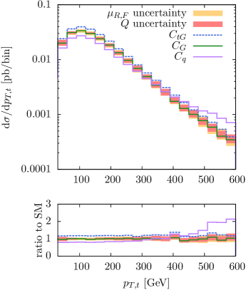
(a)

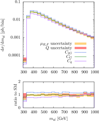
(b)

Figure 3: (a) The transverse momentum of the hardest top particle, for both the SM only, and including separately the operators of Eqs. (3.1)–(3.3), with coefficients set as in Eq. (3.5); (b) similar results for the top pair invariant mass.

In each panel of Fig. 3, the orange and red bands depict the (renormalisation and factorisation) scale and matching scale uncertainties associated with the SM result. We see in both cases that the matching uncertainty is smaller than the other scale variation, suggesting that modelling of additional radiation is well under control. Both the gluon and four-fermion operators show a shape difference with respect to the SM, albeit slight in the former case given that the gluon operator is already rather well-constrained. Nevertheless, it is difficult to gauge the statistical significance of the deviation from the SM by eye alone, and a much more quantitative description will be provided in the following section. The effect of the four-fermion operator in the $p_{T,t}$ spectrum is sizeable at large transverse momenta, as expected given that EFT operators often boost final state particles, as they contain extra momenta to offset the factor inverse new physics scale $\Lambda^{-2}$. For four-fermion operators, one may understand the enhancement as effectively arising from the lack of a SM propagator factor $1/q^{2}$. Furthermore, the transverse momentum of the hardest top particle should be particularly sensitive to the nature of additional radiation, as discussed above. Deviations are less evident, as expected, in the invariant mass spectrum, although there is still a deviation from the SM, which is worth quantifying further. Note that the dipole operator has a very similar shape to the SM contribution (as noted in Ref. [58]), but nevertheless leads to a change in overall normalisation that is still compatible with current constraints.

In Fig. 4 we show the transverse momenta of the first and second hardest additional jets, using the same conventions as Fig. 3. Again we see that the matching uncertainty is smaller than the other scale uncertainties, and that are potentially statistically significant deviations from the SM.

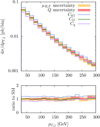
(a)

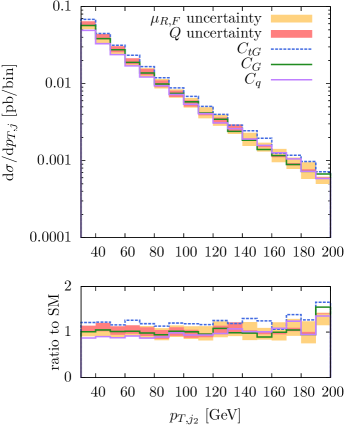
(b)

Figure 4: (a) The transverse momentum of the first hardest additional jet, for both the SM only, and including separately the operators of Eqs. (3.1)–(3.3), with coefficients set as in Eq. (3.5); (b) similar results for the second hardest additional jet.

It is interesting, however, to note that the effect of the four fermion operator is much smaller than for the transverse momentum spectrum of the hardest top particle at high $p_{T}$. This can be at least partly explained from the fact that top pair production at the LHC is dominated by the gluon channel. Thus, when only the four-fermion operator is switched on, most of the additional radiation will be purely SM-like. Another feature of Fig. 4 is that the dipole operator of Eq. (3.3) leads to a normalisation change of the jet radiation profile, but not a significant shape change. It thus mirrors the properties already observed for top-related observables in Ref. [58], that the shape of kinematic distributions involving the dipole operator is highly similar to the SM alone. Thus, we see that the transverse momenta of the additional jets are in principle useful for distinguishing the dipole and three-gluon operators, whilst providing complementary information to those observables (such as $m_{t\bar{t}}$) that also constrain four fermion operators.

In Fig. 5, we show the rapidity of the top quark, and of the hardest additional jet (similar results are obtained for the second hardest jet).

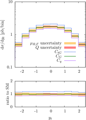
(a)

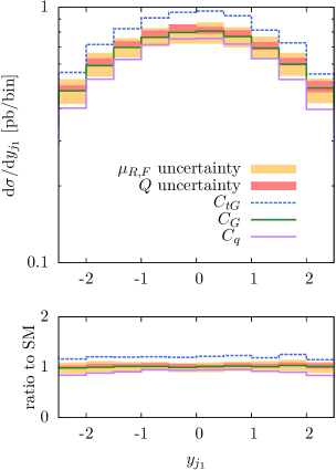
(b)

Figure 5: (a) The rapidity of the top quark, for both the SM only, and including separately the operators of Eqs. (3.1)–(3.3), with coefficients set as in Eq. (3.5); (b) similar results for the hardest additional jet.

The results are consistent with previous plots: the effect of the dipole operator is to change the normalisation of the SM contribution, but not the shape. The four fermion operator again has a smaller effect, although becomes marginally more pronounced at higher absolute rapidities, due to the fact that the parton luminosity then diminishes the gluon initiated channel.

To summarise, we have seen that EFT contributions to observables sensitive to additional radiation in top pair production indeed lead to deviations from the SM, and of comparable size to those observables (e.g. top transverse momentum, and the top pair invariant mass) that are already used in EFT fits in the top sector. Furthermore, these deviations survive against the matching and scale uncertainties associated with the SM results. How much discriminating power these extra observables have depends on the amount of data collected in coming years, but also on whether the additional jet observables are highly correlated with the top quark kinematics. We explore these issues in the following section.

3.2 Distinguishing power of jet observables

Above, we have seen that EFT operators significantly affect additional jet radiation in top pair production, such that observables involving this radiation can potentially provide useful additional constraints in global fits of top quark EFT to data. In order to check whether or not this is realised, however, we must examine the degree of correlation between observables involving the jet radiation, and those involving the top particles alone. There is clearly some degree of correlation, given that the top and antitop will recoil against additional radiation. However, it may well be the case that certain top observables are less correlated with radiation properties than others. This is then useful information for choosing optimal (i.e. the most complementary) sets of observables with which to constrain new physics.

In Fig. 6, we show two-dimensional scatter plots of the $p_{T}$ of the first hardest jet, and either the $p_{T}$ of the hardest top particle, or the top pair invariant mass. All results are calculated in the SM only.

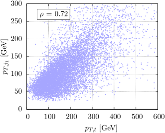
(a)

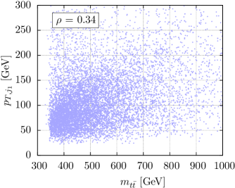
(b)

Figure 6: Scatter plots showing the transverse momentum of the hardest additional jet vs. (a) the transverse momentum of the hardest top particle; (b) the top pair invariant mass.

In each plot, we also show the Pearson correlation coefficient $\rho$. We see that the transverse momentum of the hardest top particle is more correlated with the properties of the hardest jet than the top pair invariant mass is, as expected given that the latter observable is more stable to higher order corrections. In the case of the invariant mass, the correlation coefficient is less than 0.5, suggesting that indeed the additional jet radiation is capable of providing significant complementary information relative to top properties alone. Similar plots are shown in Fig. 7 for the second hardest jet.

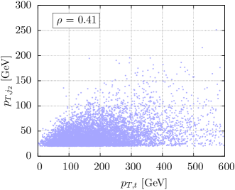
(a)

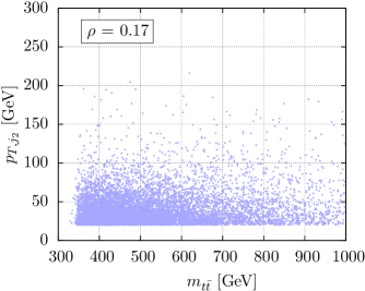
(b)

Figure 7: Scatter plots showing the transverse momentum of the second hardest additional jet vs. (a) the transverse momentum of the hardest top particle; (b) the top pair invariant mass.

Unsurprisingly, the top properties are less sensitive to the second hardest jet than they are to the first hardest jet. Again, we see that the invariant mass provides the most complementary information to the the properties of the jet radiation.

Let us now turn to the question of how sensitivity to new physics is affected by the inclusion of jet radiation observables. To estimate the gain in sensitivity, we perform a binned hypothesis test using two-dimensional distributions based on pairs of observables discussed above (in principle three-dimensional distributions carry even more shape information, but suffer from poor statistics). Our hypothesis test is based on the modified frequentist $CL_{s}$ method [117]. We take the signal hypothesis ($s$) to be each dimension six operator in turn. The background hypothesis ($b$) is the SM only, and we generate (pseudo)-data corresponding to the background, before calculating the binned log-likelihood ratio

$$q\equiv-2\log Q=-2\sum_{\begin{subarray}{c}i\end{subarray}}\left(-s_{i}+d_{i}\log\left(1+\frac{s_{i}}{b_{i}}\right)\right),$$ (3.6)

where the sum is over bins $i$, $s_{i}$ and $b_{i}$ are the expected number of signal and background values respectively, and $d_{i}$ is the number of observed events. The confidence levels for excluding the $s+b$ and $b$-only hypotheses are

$$CL_{s+b}=P_{s+b}(q>q_{obs}),\qquad CL_{b}=P_{b}(q>q_{obs}).$$ (3.7)

These represent, respectively, the probability that the test statistic $q$ would be greater than that observed in the data, given the hypothesised number of signal and background events $s+b$ or background-only events $b$. In practice, we numerically evaluate these $p$-values by generating a large number of Monte Carlo pseudo-experiments, with $CL_{s+b}$ being the fraction of pseudo-experiments that generate at least as many events as observed in the data. A signal hypothesis is regarded as excluded at the 95% confidence level if $CL_{s}\equiv CL_{s+b}/(1-CL_{b})\leq 0.05$.

To judge the usefulness of observables sensitive to additional jet radiation, we take observables $X\in\{m_{t\bar{t}},p_{T,t}\}$, and calculate the $CL_{s}$ in two cases: (i) using $X$ alone; (ii) using $X$ in combination with the transverse momentum of the first hardest jet, $p_{T,j_{1}}$. We then examine the ratio

$$\frac{CL_{s}(X,p_{T,j_{1}})}{CL_{s}(X)},$$ (3.8)

which measures the “improvement” due to including the extra radiation. We choose $p_{T,j_{1}}$ as a particular example, but similar results are obtained by choosing other radiation observables. Given that the dipole and gluon operators of Eqs. (3.2), (3.3) appear, from Figs. 3–5, to be the hardest to distinguish from the SM, we will focus on these.

Results for each operator are shown in Fig. 8, where to obtain the luminosity scale on the horizontal axis, we have multiplied all cross-sections by a factor of $6\%$, corresponding to a typical event selection efficiency for dileptonic top pair events.

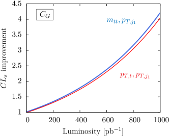
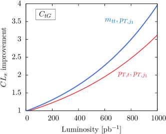
Figure 8: Relative improvement in the $CL_{s}$ for the EFT signal plus SM background, for the dipole and gluon operators of Eqs. (3.2), (3.3), when using the transverse momentum of the hardest radiated jet in additional to: the top pair invariant mass (blue line); the transverse momentum of the hardest top particle (red line).

We see in both cases that using the additional jet radiation leads to a significant improvement in the $CL_{s}$. More improvement is obtained when adding the radiation to the invariant mass distribution rather than the $p_{T}$ of the hardest top, as expected given that the former is less correlated with the radiation. More improvement is seen for the gluon operator, presumably due to the fact that this leads to a significant shape change with respect to the SM, whereas the dipole operator does not.

We did not present results for the four fermion operator of Eq. (3.1). The negative interference in some kinematic regions means that distributions involving this operator sometimes undershoot, and sometimes overshoot the SM, as can be clearly seen in Figs. 3–5. This in turn leads to cancellations in the log likelihood ratio of Eq. (3.6), so that this is not the best quantity to use to measure the advantage of using additional information. One could instead use e.g. $\chi^{2}$ values, although it is any case already clear from Figs. 3–5 that the four fermion operator typically leads to much larger deviations from the SM subject to current constraints, thereby rendering the analysis of this section less relevant.

4 Conclusion

In this paper, we have considered the issue of whether observables relating to additional jet radiation in top pair production provide a useful input to global fits of effective field theory (EFT) in the top sector. In the absence of NLO QCD corrections to processes containing EFT operators, the best way of describing such observables is to use higher order tree-level matrix elements interfaced with a parton shower. One may then worry about potential discontinuities arising from the fact that radiation generated by the matrix elements includes BSM effects, whereas radiation generated by the shower does not. We have reviewed in section 2 why this is not a problem in practice, due to the fact that the new physics contributions do not generate soft or collinear singularities.

We then studied top pair production generated at tree-level with up to two additional jets, matched to a parton shower. The matching uncertainty was found to be smaller than the factorisation and renormalisation scale uncertainty. Furthermore, deviations from the SM due to EFT operators could be observed in a number of kinematic distributions, including those associated with additional jet radiation. We quantified this in section 3.2 by looking at the relative improvement in the $CL_{s}$ for the EFT signal plus SM background, when using the $p_{T}$ of the hardest additional jet in addition to the top pair invariant mass or $p_{T}$ of the hardest top particle. We saw significant improvements, suggesting that indeed multijet observables can provide highly useful complementary information to inclusive top observables alone. The inclusion of such observables in global EFT fits is in progress.

References

- Weinberg [1979] S. Weinberg, Proceedings, Symposium Honoring Julian Schwinger on the Occasion of his 60th Birthday: Los Angeles, California, February 18-19, 1978, Physica A96, 327 (1979)\BibitemShutNoStop
- Buchmuller and Wyler [1986] W. Buchmuller and D. Wyler, Nucl. Phys. B268, 621 (1986)\BibitemShutNoStop
- Burges and Schnitzer [1983] C. J. C. Burges and H. J. Schnitzer, Nucl. Phys. B228, 464 (1983).
- Leung et al. [1986] C. N. Leung, S. T. Love, and S. Rao, Z. Phys. C31, 433 (1986).
- Hagiwara et al. [1987] K. Hagiwara, R. D. Peccei, D. Zeppenfeld, and K. Hikasa, Nucl. Phys. B282, 253 (1987).
- Grzadkowski et al. [2010] B. Grzadkowski, M. Iskrzynski, M. Misiak, and J\BibitemShut. Rosiek, JHEP 10, 085 (2010), arXiv:1008.4884 [hep-ph].
- Brivio and Trott [2017a] I. Brivio and M. Trott, (2017a), arXiv:1706.08945 [hep-ph]\BibitemShutNoStop
- Pierce et al. [2007] A. Pierce, J. Thaler, and L.-T. Wang, JHEP 05, 070 (2007), arXiv:hep-ph/0609049 [hep-ph].
- Alonso et al. [2013] R. Alonso, M. B. Gavela, L. Merlo, S. Rigolin, and J. Yepes, Phys. Rev. D87, 055019 (2013), arXiv:1212.3307 [hep-ph].
- Djouadi [2013] A. Djouadi, Eur. Phys. J. C73, 2498 (2013), arXiv:1208.3436 [hep-ph]\BibitemShutNoStop
- Low et al. [2012] I. Low, J. Lykken, and G. Shaughnessy, Phys. Rev. D86, 093012 (2012), arXiv:1207.1093 [hep-ph].
- Zhang et al. [2012] C. Zhang, N. Greiner, and S. Willenbrock, Phys. Rev. D86, 014024 (2012), arXiv:1201.6670 [hep-ph].
- Degrande [2014] C. Degrande, JHEP 02, 101 (2014), arXiv:1308.6323 [hep-ph]\BibitemShutNoStop
- Elias-Miró et al. [2013] J. Elias-Miró, J. R. Espinosa, E. Masso, and A. Pomarol, JHEP 08, 033 (2013), arXiv:1302.5661 [hep-ph].
- Contino et al. [2013] R. Contino, M. Ghezzi, C. Grojean, M. Muhlleitner, and M. Spira, JHEP 07, 035 (2013), arXiv:1303.3876 [hep-ph].
- Grojean et al. [2014] C. Grojean, E. Salvioni, M. Schlaffer, and A. Weiler, JHEP 05, 022 (2014), arXiv:1312.3317 [hep-ph].
- Gripaios and Sutherland [2014] B. Gripaios and D. Sutherland, Phys. Rev. D89, 076004 (2014), arXiv:1309.7822 [hep-ph]\BibitemShutNoStop
- Hayreter and Valencia [2013] A. Hayreter and G. Valencia, Phys. Rev. D88, 034033 (2013), arXiv:1304.6976 [hep-ph]\BibitemShutNoStop
- Buchalla et al. [2014] G. Buchalla, O. Catá, and C. Krause, Phys. Lett. B731, 80 (2014), arXiv:1312.5624 [hep-ph]\BibitemShutNoStop
- Alonso et al. [2014] R. Alonso, E. E. Jenkins, A. V. Manohar, and M. Trott, JHEP 04, 159 (2014), arXiv:1312.2014 [hep-ph].
- Gavela et al. [2015] M. B. Gavela, K. Kanshin, P. A. N. Machado, and S. Saa, JHEP 03, 043 (2015), arXiv:1409.1571 [hep-ph].
- Wells and Zhang [2014] J. D. Wells and Z. Zhang, Phys. Rev. D90, 033006 (2014), arXiv:1406.6070 [hep-ph].
- Dawson et al. [2014] S. Dawson, I. M. Lewis, and M. Zeng, Phys. Rev. D90, 093007 (2014), arXiv:1409.6299 [hep-ph].
- Delgado et al. [2014] R. L. Delgado, A. Dobado, M. J. Herrero, and J. J. Sanz-Cillero, JHEP 07, 149 (2014), arXiv:1404.2866 [hep-ph].
- Henning et al. [2016] B. Henning, X. Lu, and H. Murayama, JHEP 01, 023 (2016), arXiv:1412.1837 [hep-ph].
- Ellis et al. [2015] J. Ellis, V. Sanz, and T. You, JHEP 03, 157 (2015), arXiv:1410.7703 [hep-ph].
- Gupta et al. [2015] R. S. Gupta, A. Pomarol, and F. Riva, Phys. Rev. D91, 035001 (2015), arXiv:1405.0181 [hep-ph].
- Lehman [2014] L. Lehman, Phys. Rev. D90, 125023 (2014), arXiv:1410.4193 [hep-ph]\BibitemShutNoStop
- Englert et al. [2015] C. Englert, Y. Soreq, and M. Spannowsky, JHEP 05, 145 (2015), arXiv:1410.5440 [hep-ph].
- Corbett et al. [2015] T. Corbett, O. J. P. Eboli, D. Goncalves, J. Gonzalez-Fraile, T. Plehn, and M. Rauch, JHEP 08, 156 (2015), arXiv:1505.05516 [hep-ph].
- Chiang and Huo [2015] C.-W. Chiang and R. Huo, JHEP 09, 152 (2015), arXiv:1505.06334 [hep-ph].
- Efrati et al. [2015] A. Efrati, A. Falkowski, and Y. Soreq, JHEP 07, 018 (2015), arXiv:1503.07872 [hep-ph].
- Berthier and Trott [2015] L. Berthier and M. Trott, JHEP 05, 024 (2015), arXiv:1502.02570 [hep-ph]\BibitemShutNoStop
- Berthier and Trott [2016] L. Berthier and M. Trott, JHEP 02, 069 (2016), arXiv:1508.05060 [hep-ph]\BibitemShutNoStop
- Azatov et al. [2015] A. Azatov, R. Contino, G. Panico, and M. Son, Phys. Rev. D92, 035001 (2015), arXiv:1502.00539 [hep-ph].
- Englert et al. [2016] C. Englert, R. Kogler, H. Schulz, and M. Spannowsky, Eur. Phys. J. C76, 393 (2016), arXiv:1511.05170 [hep-ph].
- Buchalla et al. [2015] G. Buchalla, O. Cata, A. Celis, and C. Krause, Phys. Lett. B750, 298 (2015), arXiv:1504.01707 [hep-ph].
- Buchalla et al. [2016] G. Buchalla, O. Cata, A. Celis, and C. Krause, Eur. Phys. J. C76, 233 (2016), arXiv:1511.00988 [hep-ph].
- Maltoni et al. [2016] F. Maltoni, E. Vryonidou, and C. Zhang, JHEP 10, 123 (2016), arXiv:1607.05330 [hep-ph].
- Bjørn and Trott [2016] M. Bjørn and M. Trott, Phys. Lett. B762, 426 (2016), arXiv:1606.06502 [hep-ph]\BibitemShutNoStop
- Berthier et al. [2016] L. Berthier, M. Bjørn, and M. Trott, JHEP 09, 157 (2016), arXiv:1606.06693 [hep-ph].
- Englert et al. [2017] C. Englert, R. Kogler, H. Schulz, and M. Spannowsky, Eur. Phys. J. C77, 789 (2017), arXiv:1708.06355 [hep-ph].
- Brivio and Trott [2017b] I. Brivio and M. Trott, JHEP 07, 148 (2017b), [Addendum: JHEP05,136(2018)], arXiv:1701.06424 [hep-ph]\BibitemShutNoStop
- Deutschmann et al. [2017] N. Deutschmann, C. Duhr, F. Maltoni, and E. Vryonidou, JHEP 12, 063 (2017), [Erratum: JHEP02,159(2018)], arXiv:1708.00460 [hep-ph].
- de Blas et al. [2017] J. de Blas, M. Ciuchini, E. Franco, S. Mishima, M. Pierini, L. Reina, and L. Silvestrini, Proceedings, 2017 European Physical Society Conference on High Energy Physics (EPS-HEP 2017): Venice, Italy, July 5-12, 2017, PoS EPS-HEP2017, 467 (2017), arXiv:1710.05402 [hep-ph].
- Alioli et al. [2017] S. Alioli, V. Cirigliano, W. Dekens, J. de Vries, and E. Mereghetti, JHEP 05, 086 (2017), arXiv:1703.04751 [hep-ph].
- Murphy [2018] C. W. Murphy, Phys. Rev. D97, 015007 (2018), arXiv:1710.02008 [hep-ph]\BibitemShutNoStop
- de Blas et al. [2018] J. de Blas, O. Eberhardt, and C. Krause, JHEP 07, 048 (2018), arXiv:1803.00939 [hep-ph].
- Degrande et al. [2018] C. Degrande, F. Maltoni, K. Mimasu, E. Vryonidou, and C. Zhang, Submitted to: JHEP (2018), arXiv:1804.07773 [hep-ph].
- Ellis et al. [2018] J. Ellis, C. W. Murphy, V. Sanz, and T. You, JHEP 06, 146 (2018), arXiv:1803.03252 [hep-ph].
- Hays et al. [2018] C. Hays, A. Martin, V. Sanz, and J. Setford, (2018), arXiv:1808.00442 [hep-ph].
- Alves et al. [2018] A. Alves, N. Rosa-Agostinho, O. J. P. Éboli, and M. C. Gonzalez-Garcia, Phys. Rev. D98, 013006 (2018), arXiv:1805.11108 [hep-ph]\BibitemShutNoStop
- de Beurs et al. [2018] M. de Beurs, E. Laenen, M. Vreeswijk, and E. Vryonidou, (2018), arXiv:1807.03576 [hep-ph].
- Hirschi et al. [2018] V. Hirschi, F. Maltoni, I. Tsinikos, and E. Vryonidou, JHEP 07, 093 (2018), arXiv:1806.04696 [hep-ph].
- Vryonidou and Zhang [2018] E. Vryonidou and C. Zhang, JHEP 08, 036 (2018), arXiv:1804.09766 [hep-ph]\BibitemShutNoStop
- Bernlochner et al. [2018] F. U. Bernlochner, C. Englert, C. Hays, K. Lohwasser, H. Mildner, A. Pilkington, D. D. Price, and M. Spannowsky, (2018), arXiv:1808.06577 [hep-ph].
- Cao et al. [2007] Q.-H. Cao, J. Wudka, and C. P. Yuan, Phys. Lett. B658, 50 (2007), arXiv:0704.2809 [hep-ph]\BibitemShutNoStop
- Degrande et al. [2011] C. Degrande, J.-M. Gerard, C. Grojean, F. Maltoni, and G. Servant, JHEP 03, 125 (2011), arXiv:1010.6304 [hep-ph].
- Zhang and Willenbrock [2011] C. Zhang and S. Willenbrock, Phys. Rev. D83, 034006 (2011), arXiv:1008.3869 [hep-ph]\BibitemShutNoStop
- Greiner et al. [2011] N. Greiner, S. Willenbrock, and C. Zhang, Phys. Lett. B704, 218 (2011), arXiv:1104.3122 [hep-ph]\BibitemShutNoStop
- Degrande et al. [2013] C. Degrande, N. Greiner, W. Kilian, O. Mattelaer, H. Mebane, T. Stelzer, S. Willenbrock, and C. Zhang, Annals Phys. 335, 21 (2013), arXiv:1205.4231 [hep-ph]\BibitemShutNoStop
- Jung et al. [2014] S. Jung, P. Ko, Y. W. Yoon, and C. Yu, JHEP 08, 120 (2014), arXiv:1406.4570 [hep-ph].
- Dror et al. [2016] J. A. Dror, M. Farina, E. Salvioni, and J. Serra, JHEP 01, 071 (2016), arXiv:1511.03674 [hep-ph].
- Davidson et al. [2015] S. Davidson, M. L. Mangano, S. Perries, and V. Sordini, Eur. Phys. J. C75, 450 (2015), arXiv:1507.07163 [hep-ph]\BibitemShutNoStop
- Rosello and Vos [2016] M. P. Rosello and M. Vos, Eur. Phys. J. C76, 200 (2016), arXiv:1512.07542 [hep-ex]\BibitemShutNoStop
- Bessidskaia Bylund et al. [2016] O. Bessidskaia Bylund, F. Maltoni, I. Tsinikos, E. Vryonidou, and C. Zhang, JHEP 05, 052 (2016), arXiv:1601.08193 [hep-ph].
- Grzadkowski et al. [2004] B. Grzadkowski, Z. Hioki, K. Ohkuma, and J. Wudka, Nucl. Phys. B689, 108 (2004), arXiv:hep-ph/0310159 [hep-ph].
- Chen et al. [2005] C.-R. Chen, F. Larios, and C. P. Yuan, Phys. Lett. B631, 126 (2005), arXiv:hep-ph/0503040 [hep-ph].
- Aguilar-Saavedra [2009] J. A. Aguilar-Saavedra, Nucl. Phys. B812, 181 (2009), arXiv:0811.3842 [hep-ph]\BibitemShutNoStop
- Aguilar-Saavedra [2008] J. A. Aguilar-Saavedra, Nucl. Phys. B804, 160 (2008), arXiv:0803.3810 [hep-ph]\BibitemShutNoStop
- Nomura [2010] D. Nomura, JHEP 02, 061 (2010), arXiv:0911.1941 [hep-ph]\BibitemShutNoStop
- Hioki and Ohkuma [2010] Z. Hioki and K. Ohkuma, Eur. Phys. J. C65, 127 (2010), arXiv:0910.3049 [hep-ph]\BibitemShutNoStop
- Hioki and Ohkuma [2011] Z. Hioki and K. Ohkuma, Eur. Phys. J. C71, 1535 (2011), arXiv:1011.2655 [hep-ph]\BibitemShutNoStop
- Gonzalez-Sprinberg et al. [2011] G. A. Gonzalez-Sprinberg, R. Martinez, and J. Vidal, JHEP 07, 094 (2011), [Erratum: JHEP05,117(2013)], arXiv:1105.5601 [hep-ph]\BibitemShutNoStop
- Fabbrichesi et al. [2014a] M. Fabbrichesi, M. Pinamonti, and A. Tonero, Phys. Rev. D89, 074028 (2014a), arXiv:1307.5750 [hep-ph].
- Hioki and Ohkuma [2013] Z. Hioki and K. Ohkuma, Phys. Rev. D88, 017503 (2013), arXiv:1306.5387 [hep-ph].
- Aguilar-Saavedra et al. [2015] J. A. Aguilar-Saavedra, B. Fuks, and M. L. Mangano, Phys. Rev. D91, 094021 (2015), arXiv:1412.6654 [hep-ph]\BibitemShutNoStop
- Aguilar-Saavedra and Bernabeu [2010] J. A. Aguilar-Saavedra and J. Bernabeu, Nucl. Phys. B840, 349 (2010), arXiv:1005.5382 [hep-ph]\BibitemShutNoStop
- Aguilar-Saavedra et al. [2011] J. A. Aguilar-Saavedra, N. F. Castro, and A. Onofre, Phys. Rev. D83, 117301 (2011), arXiv:1105.0117 [hep-ph].
- Bernardo et al. [2014] C. Bernardo, N. F. Castro, M. C. N. Fiolhais, H. Gonçalves, A. G. C. Guerra, M. Oliveira, and A. Onofre, Phys. Rev. D90, 113007 (2014), arXiv:1408.7063 [hep-ph].
- Fabbrichesi et al. [2014b] M. Fabbrichesi, M. Pinamonti, and A. Tonero, Eur. Phys. J. C74, 3193 (2014b), arXiv:1406.5393 [hep-ph].
- Cao et al. [2015] Q.-H. Cao, B. Yan, J.-H. Yu, and C. Zhang, (2015), 10.1088/1674-1137/41/6/063101, arXiv:1504.03785 [hep-ph].
- Buckley et al. [2015] A. Buckley, C. Englert, J. Ferrando, D. J. Miller, L. Moore, M. Russell, and C. D. White, Phys. Rev. D92, 091501 (2015), arXiv:1506.08845 [hep-ph].
- Buckley et al. [2016] A. Buckley, C. Englert, J. Ferrando, D. J. Miller, L. Moore, M. Russell, and C. D. White, JHEP 04, 015 (2016), arXiv:1512.03360 [hep-ph]\BibitemShutNoStop
- Degrande et al. [2015] C. Degrande, F. Maltoni, J. Wang, and C. Zhang, Phys. Rev. D91, 034024 (2015), arXiv:1412.5594 [hep-ph].
- Buarque Franzosi and Zhang [2015] D. Buarque Franzosi and C. Zhang, Phys. Rev. D91, 114010 (2015), arXiv:1503.08841 [hep-ph]\BibitemShutNoStop
- Zhang [2016] C. Zhang, Phys. Rev. Lett. 116, 162002 (2016), arXiv:1601.06163 [hep-ph].
- Mimasu et al. [2016] K. Mimasu, V. Sanz, and C. Williams, JHEP 08, 039 (2016), arXiv:1512.02572 [hep-ph].
- Degrande et al. [2017] C. Degrande, B. Fuks, K. Mawatari, K. Mimasu, and V. Sanz, Eur. Phys. J. C77, 262 (2017), arXiv:1609.04833 [hep-ph].
- Alioli et al. [2018] S. Alioli, W. Dekens, M. Girard, and E. Mereghetti, JHEP 08, 205 (2018), arXiv:1804.07407 [hep-ph].
- D’Hondt et al. [2018] J. D’Hondt, A. Mariotti, K. Mimasu, S. Moortgat, and C. Zhang, JHEP 11, 131 (2018), arXiv:1807.02130 [hep-ph].
- Frixione and Webber [2002] S. Frixione and B. R. Webber, JHEP 06, 029 (2002), arXiv:hep-ph/0204244 [hep-ph].
- Frixione et al. [2003] S. Frixione, P. Nason, and B. R. Webber, JHEP 08, 007 (2003), arXiv:hep-ph/0305252 [hep-ph].
- Nagy and Soper [2005] Z. Nagy and D. E. Soper, JHEP 10, 024 (2005), arXiv:hep-ph/0503053 [hep-ph].
- Frixione et al. [2007] S. Frixione, P. Nason, and C. Oleari, JHEP 11, 070 (2007), arXiv:0709.2092 [hep-ph].
- Giele et al. [2008] W. T. Giele, D. A. Kosower, and P. Z. Skands, Phys. Rev. D78, 014026 (2008), arXiv:0707.3652 [hep-ph].
- Hoche et al. [2011a] S. Hoche, F. Krauss, M. Schonherr, and F. Siegert, JHEP 04, 024 (2011a), arXiv:1008.5399 [hep-ph].
- Hoche et al. [2011b] S. Hoche, F. Krauss, M. Schonherr, and F. Siegert, JHEP 08, 123 (2011b), arXiv:1009.1127 [hep-ph].
- Hoeche et al. [2012] S. Hoeche, F. Krauss, M. Schonherr, and F. Siegert, JHEP 09, 049 (2012), arXiv:1111.1220 [hep-ph].
- Catani et al. [2001] S. Catani, F. Krauss, R. Kuhn, and B. R. Webber, JHEP 11, 063 (2001), arXiv:hep-ph/0109231 [hep-ph].
- Krauss [2002] F. Krauss, JHEP 08, 015 (2002), arXiv:hep-ph/0205283 [hep-ph].
- Lonnblad [2002] L. Lonnblad, JHEP 05, 046 (2002), arXiv:hep-ph/0112284 [hep-ph].
- Lavesson and Lonnblad [2005] N. Lavesson and L. Lonnblad, JHEP 07, 054 (2005), arXiv:hep-ph/0503293 [hep-ph].
- Mangano et al. [2002] M. L. Mangano, M. Moretti, and R. Pittau, Workshop on Monte Carlo Generator Physics for Run II at the Tevatron Batavia, Illinois, April 18-20, 2001, Nucl. Phys. B632, 343 (2002), arXiv:hep-ph/0108069 [hep-ph].
- Mangano et al. [2003] M. L. Mangano, M. Moretti, F. Piccinini, R. Pittau, and A. D. Polosa, JHEP 07, 001 (2003), arXiv:hep-ph/0206293 [hep-ph].
- Ellis et al. [1996] R. K. Ellis, W. J. Stirling, and B. R. Webber, Camb. Monogr. Part. Phys. Nucl. Phys. Cosmol. 8, 1 (1996).
- Plehn [2012] T. Plehn, Lect. Notes Phys. 844, 1 (2012), arXiv:0910.4182 [hep-ph]\BibitemShutNoStop
- Krauss et al. [2017] F. Krauss, S. Kuttimalai, and T. Plehn, Phys. Rev. D95, 035024 (2017), arXiv:1611.00767 [hep-ph]\BibitemShutNoStop
- Alloul et al. [2014] A. Alloul, N. D. Christensen, C. Degrande, C. Duhr, and B. Fuks, Comput. Phys. Commun. 185, 2250 (2014), arXiv:1310.1921 [hep-ph]\BibitemShutNoStop
- Alwall et al. [2014] J. Alwall, R. Frederix, S. Frixione, V. Hirschi, F. Maltoni, O. Mattelaer, H. S. Shao, T. Stelzer, P. Torrielli, and M. Zaro, JHEP 07, 079 (2014), arXiv:1405.0301 [hep-ph].
- Sjostrand et al. [2008] T. Sjostrand, S. Mrenna, and P. Z. Skands, Comput. Phys. Commun. 178, 852 (2008), arXiv:0710.3820 [hep-ph]\BibitemShutNoStop
- Alwall et al. [2008] J. Alwall et al., Eur. Phys. J. C53, 473 (2008), arXiv:0706.2569 [hep-ph].
- Ball et al. [2013] R. D. Ball et al., Nucl. Phys. B867, 244 (2013), arXiv:1207.1303 [hep-ph]\BibitemShutNoStop
- Cacciari et al. [2008] M. Cacciari, G. P. Salam, and G. Soyez, JHEP 04, 063 (2008), arXiv:0802.1189 [hep-ph].
- Cacciari et al. [2012] M. Cacciari, G. P. Salam, and G. Soyez, Eur. Phys. J. C72, 1896 (2012), arXiv:1111.6097 [hep-ph]\BibitemShutNoStop
- Barducci et al. [2018] D. Barducci et al., (2018), arXiv:1802.07237 [hep-ph].
- Junk [1999] T. Junk, Nucl. Instrum. Meth. A434, 435 (1999), arXiv:hep-ex/9902006 [hep-ex].