Mining gold from implicit models to improve likelihood-free inference

Abstract

Simulators often provide the best description of real-world phenomena. However, the density they implicitly define is often intractable, leading to challenging inverse problems for inference. Recently, a number of techniques have been introduced in which a surrogate for the intractable density is learned, including normalizing flows and density ratio estimators. We show that additional information that characterizes the latent process can often be extracted from simulators and used to augment the training data for these surrogate models. We introduce several new loss functions that leverage this augmented data, and demonstrate that these new techniques can improve sample efficiency and quality of inference.

1 Introduction

In many areas of science, complicated real-world phenomena are best described through computer simulations. Typically, the simulators implement a stochastic generative process in the “forward” mode based on a well-motivated mechanistic model with parameters $\theta$. While the simulators can generate samples of observations $x\sim p(x|\theta)$, they typically do not admit a tractable likelihood (or density) $p(x|\theta)$. Probabilistic models defined only via the samples they produce are often called implicit models. Implicit models lead to intractable inverse problems, which is a barrier for statistical inference of the parameters $\theta$ given observed data. These problems arise in fields as diverse as particle physics, epidemiology, and population genetics, which has motivated the development of likelihood-free inference algorithms such as Approximate Bayesian Computation (ABC) [1, 2, 3, 4] and neural density estimation (NDE) techniques [5, 6, 7, 8, 9, 10, 11, 12, 13, 14, 15, 16, 17, 18, 19, 20, 21, 22, 23, 24, 25, 26, 27, 28, 29, 30, 31, 32, 33, 34]. While many of these techniques can be exact in the limit of infinite training samples, real-world simulators are computationally expensive, and sample efficiency is immensely important.

We present a suite of new techniques that can dramatically improve the sample efficiency for training neural network surrogates that estimate the likelihood $p(x|\theta)$ or likelihood ratio $r(x|\theta_{0},\theta_{1})=p(x|\theta_{0})/p(x|\theta_{1})$. This provides the key quantity needed for both frequentist and Bayesian inference procedures. Our approach involves extracting additional information that characterizes the latent process from the simulator, as we explain in Sec. 3. In Sec. 4 we introduce the loss functions that utilize this augmented data. In Sec. 5 we demonstrate through a range of experiments that these new techniques provide a significant increase in sample efficiency compared to techniques that do not leverage the augmented data, which ultimately increase the quality of inference.

2 Related work

Techniques for likelihood-free inference can be divided into two broad categories. In the first category, the inference is performed by directly comparing the observed data to the output of the simulator. This includes Approximate Bayesian Computation (ABC) [1, 2, 3, 4] and probabilistic programming systems [35, 36]. Here we focus on a second category, in which the simulator is used to generate training data for a tractable surrogate model that is used during inference. There are rich connections between simulator-based inference and learning in implicit generative models such as GANs, with a considerable amount of cross-pollination between these areas [9].

The likelihood ratio trick (LRT).

A surrogate model for the likelihood ratio $\hat{r}(x|\theta_{0},\theta_{1})$ can be defined by training a probabilistic classifier to discriminate between two equal-sized samples $\{x_{i}\}\sim p(x|\theta_{0})$ and $\{x_{i}\}\sim p(x|\theta_{1})$. The binary cross-entropy loss

$$L_{\textrm{XE}}=-\mathbb{E}[\mathds{1}(\theta=\theta_{1})\log\hat{s}(x|\theta_{0},\theta_{1})+\mathds{1}(\theta=\theta_{0})\log(1-\hat{s}(x|\theta_{0},\theta_{1}))]$$ (1)

is minimized by the optimal decision function $s(x|\theta_{0},\theta_{1})=p(x|\theta_{1})/(p(x|\theta_{0})+p(x|\theta_{1}))$. Inverting this relation, the likelihood ratio can be estimated from the classifier decision function $\hat{s}(x)$ as $\hat{r}(x|\theta_{0},\theta_{1})=(1-\hat{s}(x|\theta_{0},\theta_{1}))/\hat{s}(x|\theta_{0},\theta_{1})$. This “likelihood ratio trick” is widely appreciated [5, 6, 7, 8, 9, 10, 11, 12, 13]. In practice, not all probabilistic classifiers trained to separate samples from $\theta_{0}$ and $\theta_{1}$ learn the optimal decision function. As long as the classifier decision function is a monotonic function of the likelihood ratio, this relation can be restored through a calibration procedure, substantially increasing the applicability of the likelihood ratio trick [6, 7, 8]. We use the term Carl (Calibrated approximate ratios of likelihoods) to describe likelihood ratio estimators based on calibrated classifiers.

Neural density estimation (NDE).

More recently, several methods for conditional density estimation have been proposed, often based on neural networks [14, 15, 16, 17, 18, 19, 20, 21, 22, 23, 24, 25, 26, 27, 28, 29, 30, 31, 13, 32, 33, 34]. They can be used to train a surrogate for the likelihood $p(x|\theta)$ [17, 19, 34] or, in a Bayesian setting, the posterior $p(\theta|x)$ [29, 33, 37]. One particularly interesting class of models are normalizing flows [14, 15, 16, 17, 18, 19, 20, 21, 22], which model the density as a sequence of invertible transformations applied to a simple base density. The target density is then given by the Jacobian determinant of the transformation. Closely related, autoregressive models [23, 24, 25, 26, 27] factorize a target density as a sequence of simpler conditional densities.

Novel contributions.

The most important novel contribution that differentiates our work from the existing methods is the observation that additional information can be extracted from the simulator, and the development of loss functions that allow us to use this “augmented” data to more efficiently learn surrogates for the likelihood function. In addition, we show how the augmented data can be used to define locally optimal summary statistics, which can then be used for inference with density estimation techniques or ABC. We playfully introduce the analogy of mining gold as this augmented data requires work to extract and is very valuable. In experiments we demonstrate that these approaches can dramatically improve sample efficiency and quality of likelihood-free inference.

Concurrently, the application of these methods to a specific class of problems in particle physics has been discussed in Refs. [38, 39]. The present manuscript is meant to serve as the primary reference for these new techniques and is addressed to the broader physical science and machine learning communities. Most importantly, it generalizes the specific particle physics case to almost any scientific simulator, requiring significantly weaker assumption than those made in the physics context. We also introduce an entirely new algorithm called Scandal, for which we provide the first experimental results.

3 Extracting more information from the simulator

We consider a scientific simulator that implements a stochastic generative process that proceeds through a series of latent states $z_{i}\in\mathcal{Z}_{i}$ and finally to an output $x\in\mathbb{R}^{d_{x}}$. The latent space structure $\mathcal{Z}$ can involve discrete and continuous components and is derived from the control flow of the (differentiable or non-differentiable) simulation code. Based on the mechanistic model implemented by the simulator, each latent state is sampled from a conditional probability density $z_{i}\sim p_{i}(z_{i}|\theta,z_{<i})$ and the final output is sampled from $x\sim p_{x}(x|\theta,z)$. The likelihood is then given by

$$p(x|\theta)=\int\!\mathrm{d}z\;p(x,z|\theta)=\int\!\mathrm{d}z\;p_{x}(x|\theta,z)\;\prod_{i}p_{i}(z_{i}|\theta,z_{<i})\,.$$ (2)

Often the likelihood is intractable exactly because the latent space $z$ is enormous and it is unfeasible to explicitly calculate this integral. In real-world scientific simulators, the trajectory for a single observation can involve many millions of latent variables.

In this paper we consider the problem of estimating the likelihood $p(x|\theta)$ or the likelihood ratio $r(x|\theta_{0},\theta_{1})$, which for the practical purpose of inferring parameter values $\theta$ can be used almost interchangably, based on the data available from $N$ runs of the simulator.

Typically, the setting of likelihood-free inference assumes that the only available output from the simulator are samples of observations $x\sim p(x|\theta)$. But in real-life simulators, more information can usually be extracted. We typically have access to the latent variables $z$, and the distributions of each latent variable $p_{i}(z_{i}|\theta,z_{<i})$ and $p_{x}(x|\theta,z)$ are tractable.

The key observation that is the starting point of our new inference methods is the following: While $p(x|\theta)$ is intractable, for each simulated sample we can calculate the joint score

$$t(x,z|\theta_{0})\equiv\nabla_{\theta}\log p(x,z|\theta)\biggr{|}_{\theta_{0}}=\sum_{i}\nabla_{\theta}\log p_{i}(z_{i}|\theta,z_{<i})\biggr{|}_{\theta_{0}}+\nabla_{\theta}\log p_{x}(x|\theta,z)\biggr{|}_{\theta_{0}}$$ (3)

by accumulating the factors $\nabla_{\theta}\log p(z_{i}|\theta,z_{:i})$ as the simulation runs forward through its control flow conditioned on the random trajectory $z$. It can be insightful to think of the mechanistic model in the simulator as defining a policy $\pi_{\theta}$ and $t(x,z|\theta_{0})$ as analogous to the policy gradient used in Reinforce [40]. However, instead of trying to optimize $\theta$ via a stochastic gradient estimate of some reward function, we will simply augment the data generated by the simulator with the joint score.

Similarly, we can extract the joint likelihood ratio

$$r(x,z|\theta_{0},\theta_{1})\equiv\frac{p(x,z|\theta_{0})}{p(x,z|\theta_{1})}=\frac{p_{x}(x|\theta_{0},z)}{p_{x}(x|\theta_{1},z)}\;\prod_{i}\frac{p_{i}(z_{i}|\theta_{0},z_{<i})}{p_{i}(z_{i}|\theta_{1},z_{<i})}\,.$$ (4)

The joint score and joint likelihood ratio quantify how much more or less likely a particular simulated trajectory through the simulator would be if one changed $\theta$.

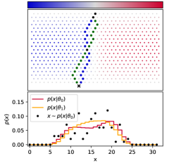
Figure 1: A toy simulation generalizing the Galton board where the transitions are biased left (blue) or right (red) depending on the nail position and the value of $\theta$. Two example latent trajectories $z$ are shown (blue and green), leading to the same observed value of $x$. Below, the distribution for $\theta_{0}=-0.8$ and $\theta_{1}=-0.6$. An example empirical distribution from 100 runs for $\theta_{0}$ shows that the sample variance is much larger than the differences from $\theta_{0}$ vs $\theta_{1}$.

As a motivating example, consider the simulation for a generalization of the Galton board, in which a set of balls is dropped through a lattice of nails ending in one of several bins denoted by $x$. The Galton board is commonly used to demonstrate the central limit theorem, and if the nails are uniformly placed such that the probability of bouncing to the left is $p$, the sum over the latent space is tractable analytically and the resulting distribution of $x$ is a binomial distribution. However, if the nails are not uniformly placed, and the probability of bouncing to the left is an arbitrary function of the nail position and some parameter $\theta$, the resulting distribution requires an explicit sum over the latent paths $z$ that might lead to a particular $x$. Such a distribution would become intractable as the size of the lattice increases. Figure 1 shows an example of two latent trajectories that lead to the same $x$. In this toy example, the probability $p(z_{h},z_{v},\theta)$ of going left is given by $(1-f(z_{v}))/2+f(z_{v}){\sigma}(5\theta(z_{h}-\nicefrac{{1}}{{2}}))$, where $f(z_{v})=\sin(\pi z_{v})$, $\sigma$ is the sigmoid function, and $z_{h}$ and $z_{v}$ are the horizontal and vertical nail positions normalized to $[0,1]$. This leads to a non-trivial $p(x|\theta)$, which can even be bimodal. Code for simulation and inference in this problem is available at Ref. [41].

Figure 1 shows that a large number of samples from the simulator are needed to reveal the differences in the distribution of $x$ for small changes in $\theta$ – the number of samples needed grows like $(p/\Delta p)^{2}$. Moreover, this toy simulation is representative of many real-world simulators in that it is composed of non-differentiable control-flow elements. This poses a difficulty, making methods based on $\nabla_{z}x$ [42] and $\nabla_{\theta}x$ inapplicable, which previously motivated techniques such as Adversarial Variational Optimization [32]. But the joint score in Eq. (3) can easily be computed by accumulating the factors $\nabla_{\theta}\log p(z_{h},z_{v}|\theta_{0})$, and we can calculate the joint likelihood ratio by accumulating factors $p(z_{h},z_{v}|\theta_{0})/p(z_{h},z_{v}|\theta_{1})$. In analogy to the Galton board toy example, even complicated real-world simulators often allow us to accumulate these factors as they run, and to calculate the joint score and joint likelihood ratio conditional on a particular stochastic execution trace $z$. We will demonstrate this with two more examples in Sec. 5.

For simulators written in an automatic differentiation framework, the calculation of the joint score and joint likelihood ratio can be entirely automatic and does not require any changes to the simulator code and output. As a proof of principle, at Ref. [43] we provide a framework that automates these calculations for any simulator in which all stochastic steps are implemented with the Pyro library [44].

4 Learning from augmented data

4.1 Key idea

How can the “augmented data” consisting of simulated observations ${x_{i}}$, the joint likelihood ratio $r(x_{i},z_{i}|\theta_{0},\theta_{1})$, and the joint score $t(x_{i},z_{i}|\theta_{0})$ be used to estimate the likelihood $p(x|\theta)$ or likelihood ratio $r(x|\theta_{0},\theta_{1})$? The relation between $r(x,z|\theta_{0},\theta_{1})$ and $r(x|\theta_{0},\theta_{1})$ is not trivial — the integral of the ratio is not the ratio of the integrals! Similarly, how can the joint score be used to estimate the intractable score function

$$t(x|\theta_{0})\equiv\nabla_{\theta}\log p(x|\theta)\biggr{|}_{\theta_{0}}\,?$$ (5)

The integral of the log is not the log of the integral!

Consider the squared error of a function $\hat{g}(x)$ that only depends on the observable $x$, but is trying to approximate a function $g(x,z)$ that also depends on the latent variable $z$,

$$L_{\textrm{MSE}}=\mathbb{E}_{p(x,z|\theta)}\left[\;\left(g(x,z)-\hat{g}(x)\right)^{2}\,\right].$$ (6)

The minimum-mean-squared-error prediction of $\hat{g}(x)$ is given by the conditional expectation $g^{*}(x)=\operatorname*{arg\,min}_{\hat{g}}L_{\textrm{MSE}}=\mathbb{E}_{p(z|x,\theta)}[g(x,z)]$.

Identifying $g(x,z)$ with the joint likelihood ratio $r(x,z|\theta_{0},\theta_{1})$ and $\theta=\theta_{1}$, we define

$$L_{r}=\mathbb{E}_{p(x,z|\theta_{1})}\left[\;\left(r(x,z|\theta_{0},\theta_{1})-\hat{r}(x)\right)^{2}\,\right]\,,$$ (7)

and find that this functional is minimized by $r^{*}(x)=\operatorname*{arg\,min}_{\hat{r}}L_{r}=\mathbb{E}_{p(z|x,\theta_{1})}\left[\,r(x,z|\theta_{0},\theta_{1})\,\right]=r(x|\theta_{0},\theta_{1})$. Similarly, by identifying $g(x,z)$ with the joint score $t(x,z|\theta_{0})$ and setting $\theta=\theta_{0}$, we define

$$L_{t}=\mathbb{E}_{p(x,z|\theta_{0})}\left[\;\left(t(x,z|\theta_{0})-\hat{t}(x|\theta_{0})\right)^{2}\,\right]\,,$$ (8)

which is minimized by $t^{*}(x)=\mathbb{E}_{p(z|x,\theta_{0})}\left[\,t(x,z|\theta_{0})\,\right]=t(x|\theta_{0})$.

These loss functionals are immensely useful because they allow us to transform $t(x,z|\theta_{0})$ into $t(x|\theta_{0})$ and $r(x,z|\theta_{0},\theta_{1})$ into $r(x|\theta_{0},\theta_{1})$: we are able to regress on these two intractable quantities! This is what makes the joint score and joint likelihood ratio the gold worth mining.

4.2 Learning the likelihood ratio

Based on this observation we introduce a family of new likelihood-free inference techniques. They fall into two categories. We first discuss a class of algorithms that uses the augmented data to learn a surrogate model for any likelihood $p(x|\theta)$ or likelihood ratio $r(x|\theta_{0},\theta_{1})$. In Section 4.3 we will define a second class of methods that is based on a local expansion of the model around some reference parameter point.

The simulators we consider in this work do not only implicitly define a single density $p(x)$, but a family of densities $p(x|\theta)$. The parameters $\theta$ may potentially belong to a high-dimensional parameter space. For inference models based on surrogate models, there are two broad strategies to model this dependence. The first is to estimate $p(x|\theta)$ or the likelihood ratio $r(x|\theta_{0},\theta_{1})$ for specific values of $\theta$ or pairs $(\theta_{0},\theta_{1})$. This may be done via a pre-defined set of $\theta$ values or on-demand using an active-learning iteration. We follow a second approach, in which we train parameterized estimators for the full model $\hat{p}(x|\theta)$ or $\hat{r}(x|\theta_{0},\theta_{1})$ as a function of both the observables $x$ and the parameters $\theta$ [6, 45]. The training data then consists of a number of samples, each generated with different values of $\theta_{0}$ and $\theta_{1}$, and the parameter values are used as additional inputs to the surrogate model. When modeling the likelihood ratio, the reference hypothesis $\theta_{1}$ in the denominator of the likelihood ratio can be kept at a fixed reference value (or a marginal model with some prior $\pi(\theta_{1})$), and only the $\theta_{0}$ dependence is modeled by the network. This approach encourages the estimator to learn the typically smooth dependence of the likelihood ratio on the parameters of interest from the training data and borrow power from neighboring points.

Rolr (Regression On Likelihood Ratio):

First, a number of parameter points $(\theta_{0},\theta_{1})$ is drawn from $\theta_{i}\sim\pi_{i}(\theta_{i})$. For each pair $(\theta_{0},\theta_{1})$, we run the simulator both for $\theta_{0}$ and for $\theta_{1}$, labelling the samples with $y=0$ and $y=1$, respectively. In addition to samples $x\sim p(x|\theta_{y})$ we also extract the joint likelihood ratio $r(x,z|\theta_{0},\theta_{1})$.

An expressive regressor $\hat{r}(x|\theta_{0},\theta_{1})$ (e. g. a neural network) is trained by minimizing the squared error loss

$$L_{\textsc{Rolr}}[\hat{r}]=\frac{1}{N}\sum_{i}\Biggl{(}y_{i}\,|r(x_{i},z_{i})-\hat{r}(x_{i})|^{2}+(1-y_{i})\,\left|\frac{1}{r(x_{i},z_{i})}-\frac{1}{\hat{r}(x_{i})}\right|^{2}\Biggr{)}.$$ (9)

Here and in the following the $\theta$ dependence is implicit to reduce the notational clutter.

Both terms in this loss function are estimators of Eq. (7) (in the second term we switch $\theta_{0}\leftrightarrow\theta_{1}$ to reduce the variance by mapping out other regions of $x$ space). As we showed in the previous section, this loss function is, at least in the limit of infinite data, minimized by the true likelihood ratio $r(x|\theta_{0},\theta_{1})$. A regressor trained in this way thus provides an estimator for the likelihood ratio and can be used for frequentist or Bayesian inference methods.

Rascal (Ratio And SCore Approximate Likelihood ratio):

If such a likelihood ratio regressor is differentiable (as is the case for neural networks) with respect to $\theta$, we can calculate the predicted score $\hat{t}(x|\theta_{0})=\nabla_{\theta_{0}}\log\hat{r}(x|\theta_{0},\theta_{1})$. For a perfect likelihood ratio estimator, $\hat{t}(x|\theta_{0})$ minimizes the squared error with respect to the joint score, see Eq. (8). Turning this argument around, we can improve the training of a likelihood ratio estimator by minimizing the combined ratio and score loss with a hyper-parameter $\alpha$

$$L_{\textsc{Rascal}}[\hat{r}]=L_{\textsc{Rolr}}[\hat{r}]+\alpha\frac{1}{N}\sum_{i}(1-y_{i})\left|t(x_{i},z_{i})-\nabla_{\theta_{0}}\log\hat{r}(x_{i})\right|^{2}\;.$$ (10)

Cascal (Carl And SCore Approximate Likelihood ratio):

The same trick can be used to improve the likelihood ratio trick and the Carl inference method [6, 8]. Following the discussion around Eq. (1), a calibrated classifier trained to discriminate samples $\{x_{i}\}\sim p(x|\theta_{0})$ and $\{x_{i}\}\sim p(x|\theta_{1})$ provides a likelihood ratio estimator. For a differentiable parameterized classifier, we can calculate the surrogate score $\hat{t}(x|\theta_{0})=\nabla_{\theta_{0}}\log[(1-\hat{s}(x|\theta_{0},\theta_{1}))/\hat{s}(x|\theta_{0},\theta_{1})]$. This allows us to train an improved classifier (and thus a likelihood ratio estimator) by minimizing the combined loss

$$L_{\textsc{Cascal}}[\hat{s}]=L_{\mathrm{XE}}[\hat{s}]+\alpha\frac{1}{N}\sum_{i}(1-y_{i})\left|t(x_{i},z_{i})-\nabla_{\theta_{0}}\log\left[\frac{1-\hat{s}(x)}{\hat{s}(x)}\right]\right|^{2}\,.$$ (11)

Scandal (SCore-Augmented Neural Density Approximates Likelihood):

Finally, we can use the same strategy to improve conditional neural density estimators such as density networks or normalizing flows. If a parameterized neural density estimator $\hat{p}(x|\theta)$ is differentiable with respect to $\theta$, we can calculate the surrogate score $\hat{t}(x)=\nabla_{\theta}\log\hat{p}(x|\theta)$ and train an improved density estimator by minimizing

$$L_{\textsc{Scandal}}[\hat{p}]=L_{\mathrm{MLE}}+\alpha\frac{1}{N}\sum_{i}\left|t(x_{i},z_{i})-\nabla_{\theta}\log\hat{p}(x)\right|^{2}\,.$$ (12)

Unlike the methods discussed before, this provides an estimator of the likelihood itself rather than its ratio. Depending on the architecture, the surrogate also provides a generative model.

4.3 Locally sufficient statistics for implicit models

A second class of new likelihood-free inference methods is based on an expansion of the implicit model around a reference parameter point $\theta_{\text{ref}}$. Up to linear order in $\theta-\theta_{\text{ref}}$, we find

$${p_{\text{local}}}(x|\theta)=\frac{1}{Z(\theta)}\,p(t(x|\theta_{\text{ref}})\,|\,\theta_{\text{ref}})\,\exp[t(x|\theta_{\text{ref}})\cdot(\theta-\theta_{\text{ref}})]$$ (13)

with some normalization factor $Z(\theta)$. This local approximation is in the exponential family and the score vector $t(x|\theta_{\text{ref}})$, defined in Eq. (5), are its sufficient statistics.

For inference in a sufficiently small neighborhood around a reference point $\theta_{\text{ref}}$, a precise estimator of the score $\hat{t}(x|\theta_{\text{ref}})$ therefore defines a vector of ideal summary statistics that contain all the information in an observation $x$ on the parameters $\theta$ [see also 46, 3, 47]. The joint score together with a minimization of the loss in Eq. (8) allows us to extract sufficient statistics from an intractable, non-differentiable simulator, at least in the neighborhood of $\theta_{\text{ref}}$. Moreover, this local model can be estimated by running the simulator at a single value $\theta_{\text{ref}}$ — it does not require scanning the $\theta$ space, and thus avoids the curse of dimensionality. Based on this observation, we introduce two further inference strategies:

Sally (Score Approximates Likelihood LocallY):

By minimizing the squared error with respect to the joint score, see Eq. (8), we train a score estimator $\hat{t}(x|\theta_{\text{ref}})$. In a next step, we estimate the density $\hat{p}(\hat{t}(x|\theta_{\text{ref}})|\theta)$ through standard multivariate density estimation techniques. This calibration procedure implicitly includes the effect of the normalizing constant $Z(\theta)$.

Sallino (Score Approximates Likelihood Locally IN One dimension):

The Sally inference method requires density estimation in the estimated score space, with typically $\dim\hat{t}\equiv\dim\theta\ll\dim x$. But in cases with large number of parameters, it is beneficial to reduce the dimensionality even further. In the local model of Eq. (13), the likelihood ratio $r(x|\theta_{0},\theta_{1})$ only depends on $h(x|\theta_{0},\theta_{1})\equiv t(x|\theta_{\text{ref}})\cdot(\theta_{0}-\theta_{1})$ up to an $x$-independent constant related to $Z(\theta)$. Any neural score estimator lets us also estimate this scalar function, which is a sufficient statistic for the 1-dimensional parameter space connecting $\theta_{0}$ and $\theta_{1}$. We can thus estimate the likelihood ratio through univariate, rather than multivariate, density estimation on $\hat{h}$.

The Sally and Sallino techniques are designed to work very well close to the reference point. The local model approximation may deteriorate further away, leading to a reduced sensitivity and weaker bounds. These approaches are simple and robust, and in particular the Sallino algorithm scales exceptionally well to high-dimensional parameter spaces.

For all these inference strategies, the augmented data is particularly powerful for enhancing the power of simulation-based inference for small changes in the parameter $\theta$. When restricted to samples $x\sim p(x|\theta)$, the variance from the simulator is a challenge. The fluctuations in the empirical density scale with the square root of the number of samples, thus large numbers of samples are required before small changes in the implicit density can faithfully be distinguished. In contrast, each sample of the joint ratio and joint score provides an exact piece of information even for arbitrarily small changes in $\theta$. On the other hand, the augmented data is less powerful for deciding between model parameter points that are far apart. In this situation the joint probability distributions $p(x,z|\theta)$ often do not overlap significantly, and the joint likelihood ratio can have a large variance around the intractable likelihood ratio $r(x|\theta_{0},\theta_{1})$. In addition, over large distances in parameter space the local model is not valid and the score does not characterize the likelihood ratios anymore, limiting the usefulness of the joint score.

5 Experiments

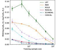
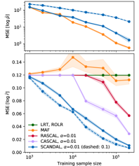
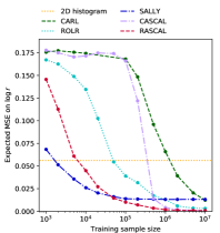
Figure 2: Left: Galton board example. MSE on $\log r$ vs. training sample size. We show the mean and its error based on 15 runs. Middle: Lotka-Volterra example. MSE on $\log p$ (top) and $\log r$ (bottom) vs. training sample size. We show the median and the standard deviation of 10 runs. Right: Particle physics example. MSE on $\log r$ vs. training sample size.

Generalized Galton board.

We return to the motivating example in Sec. 3 and Fig. 1 and try to estimate likelihood ratios for the generalized Galton board. We use the likelihood ratio trick and a neural density estimator as baselines and compare them to the new Rolr, Rascal, Cascal, and Scandal methods. As the simulator defines a distribution over a discrete $x$, for the NDE and Scandal methods we use a neural network with a softmax output layer over the bins to model $\hat{p}(x|\theta)$. All networks are explicitly parameterized in terms of $\theta$, the parameter of the simulator that defines the position of the nails (i. e. they take $\theta$ as an input). We use a simple network architecture with a single hidden layer, 10 hidden units, and $\tanh$ activations. The left panel of Fig. 2 shows the mean squared error between $\log\hat{r}(x|\theta_{0},\theta_{1})$ and the true $\log{r}(x|\theta_{0},\theta_{1})$ (estimated from histograms of $2\cdot 10^{4}$ simulations from $\theta_{0}\!=\!\!-0.8$ and $\theta_{1}\!=\!\!-0.6$), summing over $x\in[5,15]$, versus the training sample size (which refers to the total number of $x$ samples, distributed over 10 values of $\theta\in[-1,-0.4]$). We find that both Scandal and Rascal are dramatically more sample efficient than pure neural density estimation and the likelihood ratio trick, which do not leverage the joint score. Rolr improves upon pure neural density estimation and achieves the same asymptotic error as Scandal, though more slowly.

Lotka-Volterra model.

As a second example, we consider the Lotka-Volterra system [48, 49], a common example in the likelihood-free inference literature. This stochastic Markov jump process models the dynamics of a species of predators interacting with a species of prey. Four parameters $\theta$ set the rate of predators and prey being born, predators dying, and predators eating prey.

We simulate the Lotka-Volterra model with Gillespie’s algorithm [50]. From the time evolution of the predator and prey populations we calculate summary statistics $x\in\mathbb{R}^{9}$. Our model definitions, summary statistics, and initial conditions exactly follow Appendix F of Ref. [29]. In addition to the observations, we extract the joint score as well as the joint likelihood ratio with respect to a reference hypothesis $\log\theta_{1}=(-4.61,-0.69,0.00,-4.61)^{T}$ from the simulator. On this augmented data we train different likelihood and likelihood ratio estimators. As baselines we use Carl [6, 8] and a conditional masked autoregressive flow (MAF) [17, 51]. We compare them to the new techniques introduced in section 4.2, including a Scandal likelihood estimator based on a MAF. For MAF and Scandal we stack four masked autoregressive distribution estimators (MADEs) [23] on a mixture of MADEs with 10 components [17]. For all other methods, we use three hidden layers. In all cases, the hidden layers have 100 units and $\tanh$ activations. Code for simulation and inference is available at Ref. [52].

For inference on a wide prior in the parameter space, the different probability densities often do not overlap. As discussed above, the augmented data is then of limited use. Instead, we focus on the regime where we try to discriminate between close parameter points with similar predictions for the observables. We generate training data and evaluate the models in the range $\log(\theta_{1})_{i}-0.01\leq\theta_{i}\leq\log(\theta_{1})_{i}+0.01$ with a uniform prior in log space. In the middle panel of Fig. 2 we evaluate the different methods by calculating the mean squared error of estimators trained on small training samples. Since the true likelihood is intractable, we calculate the error with respect to the median predictions of 10 estimators trained on the full data set of 200 000 samples.

Our results indicate a trade-off between the performance in likelihood (density) estimation and likelihood ratio estimation. For density estimation, the MAF performs well. The variance of the score term in the Scandal loss degrades the performance, especially for larger values of the hyperparameter $\alpha$. However, for statistical inference the more relevant quantity is the likelihood ratio. Here the new techniques that use the joint score, in particular Scandal, are significantly more sample efficient.

Particle physics.

Finally we consider a real-world problem from particle physics. A simulator describes the production of a Higgs boson at the Large Hadron Collider experiments, followed by the decay into four electrons or muons, subsequent radiation patterns, the interaction with the detector elements, and the reconstruction procedure. Each recorded collision produces a single high-dimensional observable $x\in\mathbb{R}^{42}$, and the dataset consists of multiple iid observations of $x$. The goal is to infer the likelihood of two parameters $\theta\in[-1,1]^{2}$ that characterize the effect of high-energy physics models on these interactions. We consider a synthetic observed dataset with 36 iid simulated observations of $x$ drawn from $\theta=(0,0)$.

The new inference techniques can accommodate state-of-the-art simulators, but in that setting we cannot compare them to the true likelihood function. We therefore present a simplified setup and approximate the detector response such that the true likelihood function is tractable, providing us with a ground truth to compare the inference techniques to. As simulator we use a combination of MadGraph 5 [53] and MadMax [54, 55, 56]. The setup and the results of this experiment are described at length in Ref. [39], which is attached as supplementary material.

In the right panel of Fig. 2 we show the expected mean squared error of the approximate $\log\hat{r}(x|\theta_{0},\theta_{1})$ for the different techniques as a function of the training sample size. We take the expectation over random values of $\theta_{0}$, drawn from a Gaussian prior with mean $(0,0)$ and covariance matrix $\operatorname{diag}(0.2^{2},0.2^{2})$. We compare the new techniques to the standard practice in particle physics, in which the likelihood is estimated through histograms of two hand-picked summary statistics.

All new inference techniques outperform the traditional histogram method, provided that the training samples are sufficiently large. Using augmented data substantially decreases the amount of training data required for a good performance: the Rascal method, which uses both the joint ratio and joint score information from the simulator, reduces the amount of training data by two orders of magnitude compared to the Carl technique, which uses only the samples $x\sim p(x|\theta)$. The particularly simple local techniques Sally and Sallino need even less data for a good performance. However, their performance eventually plateaus and does not asymptote to zero error. This is because the local model approximation breaks down further away from the reference point $\theta_{\text{ref}}=(0,0)^{T}$, and the score is no longer the sufficient statistics. In the supplementary material we show further results and demonstrate how the improved likelihood ratio estimation leads to better inference results.

6 Conclusions

In this work we have presented a family of new inference techniques for the setting in which the likelihood is only implicitly defined through a stochastic generative simulator. The new methods estimate likelihoods or ratios of likelihoods with data available from the simulator. Most established inference methods, such as ABC and techniques based on neural density estimation, only use samples of observables from the simulator. We pointed out that in many cases the joint likelihood ratio and the joint score — quantities conditioned on the latent variables that characterize the trajectory through the data generation process — can be extracted from the simulator.

While these additional quantities often require work to be extracted, they also prove to be very valuable as they can dramatically improve sample efficiency and quality of inference. Indeed, we have shown that this additional information lets us define loss functionals that are minimized by the likelihood or likelihood ratio, which can in turn be used to efficiently guide the training of neural networks to precisely estimate the likelihood function. A second class of new techniques is motivated by a local approximation of the likelihood function around a reference parameter value, where the score vector is the sufficient statistic. In the case where the simulator provides the joint score, we can use it to train a precise estimator of the score and use it as locally optimal summary statistics.

We have demonstrated in three experiments that the new inference techniques let us precisely estimate likelihood ratios. In turn, this enables parameter measurements with a higher precision and less training data than with established methods.

This approach is complementary to many recent advances in likelihood-free inference: the augmented data can be used to improve training for any neural density estimator or likelihood ratio estimator, as we have demonstrated for Masked Autoregressive Flows and Carl. It can also be used to define locally optimal summary statistics that can be used for instance in ABC techniques.

Finally, these results motivate the development of tools that provide a nonstandard interpretation of the simulator code and automatically generate the joint score and joint ratio, building on recent developments in probabilistic programming and automatic differentiation [57, 58, 59, 36, 60, 35]. We have provided a first proof-of-principle implementation of such a tool based on Pyro [43].

Acknowledgments

We would like to thank Cyril Becot and Lukas Heinrich, who contributed to this project at an early stage. We are grateful to Jan-Matthis Lückmann for helping us automate the calculation of the joint likelihood ratio and joint score in Pyro and to all participants of the Likelihood-free inference workshop at the Flatiron Institute for great discussions. We would like to thank Felix Kling, Tilman Plehn, and Peter Schichtel for providing the MadMax code and helping us use it, and to George Papamakarios for discussing the Masked Autoregressive Flow code with us. KC wants to thank CP3 at UC Louvain for their hospitality. Finally, we would like to thank Atılım Güneş Baydin, Lydia Brenner, Joan Bruna, Kyunghyun Cho, Michael Gill, Siavash Golkar, Ian Goodfellow, Daniela Huppenkothen, Michael Kagan, Hugo Larochelle, Yann LeCun, Fabio Maltoni, Jean-Michel Marin, Iain Murray, George Papamakarios, Duccio Pappadopulo, Dennis Prangle, Rajesh Ranganath, Dustin Tran, Rost Verkerke, Wouter Verkerke, Max Welling, and Richard Wilkinson for interesting discussions.

JB, KC, and GL are grateful for the support of the Moore-Sloan data science environment at NYU. KC and GL were supported through the NSF grants ACI-1450310 and PHY-1505463. JP was partially supported by the Scientific and Technological Center of Valparaíso (CCTVal) under Fondecyt grant BASAL FB0821. This work was supported in part through the NYU IT High Performance Computing resources, services, and staff expertise.

References

- [1] D. B. Rubin: ‘Bayesianly justifiable and relevant frequency calculations for the applied statistician’. Ann. Statist. 12 (4), p. 1151, 1984. URL https://doi.org/10.1214/aos/1176346785.
- [2] M. A. Beaumont, W. Zhang, and D. J. Balding: ‘Approximate bayesian computation in population genetics’. Genetics 162 (4), p. 2025, 2002.
- [3] J. Alsing, B. Wandelt, and S. Feeney: ‘Massive optimal data compression and density estimation for scalable, likelihood-free inference in cosmology’ , 2018. arXiv:1801.01497.
- [4] T. Charnock, G. Lavaux, and B. D. Wandelt: ‘Automatic physical inference with information maximizing neural networks’. Phys. Rev. D97 (8), p. 083004, 2018. arXiv:1802.03537.
- [5] I. J. Goodfellow, J. Pouget-Abadie, M. Mirza, et al.: ‘Generative Adversarial Networks’. ArXiv e-prints , 2014. arXiv:1406.2661.
- [6] K. Cranmer, J. Pavez, and G. Louppe: ‘Approximating Likelihood Ratios with Calibrated Discriminative Classifiers’ , 2015. arXiv:1506.02169.
- [7] K. Cranmer and G. Louppe: ‘Unifying generative models and exact likelihood-free inference with conditional bijections’. J. Brief Ideas , 2016.
- [8] G. Louppe, K. Cranmer, and J. Pavez: ‘carl: a likelihood-free inference toolbox’. J. Open Source Softw. , 2016.
- [9] S. Mohamed and B. Lakshminarayanan: ‘Learning in Implicit Generative Models’. ArXiv e-prints , 2016. arXiv:1610.03483.
- [10] M. U. Gutmann, R. Dutta, S. Kaski, and J. Corander: ‘Likelihood-free inference via classification’. Statistics and Computing p. 1–15, 2017.
- [11] T. Dinev and M. U. Gutmann: ‘Dynamic Likelihood-free Inference via Ratio Estimation (DIRE)’. arXiv e-prints arXiv:1810.09899, 2018. arXiv:1810.09899.
- [12] J. Hermans, V. Begy, and G. Louppe: ‘Likelihood-free MCMC with Approximate Likelihood Ratios’ , 2019. arXiv:1903.04057.
- [13] D. Tran, R. Ranganath, and D. Blei: ‘Hierarchical implicit models and likelihood-free variational inference’. In I. Guyon, U. V. Luxburg, S. Bengio, et al. (eds.), ‘Advances in Neural Information Processing Systems 30’, p. 5523–5533, 2017.
- [14] L. Dinh, D. Krueger, and Y. Bengio: ‘NICE: Non-linear Independent Components Estimation’. ArXiv e-prints , 2014. arXiv:1410.8516.
- [15] D. Jimenez Rezende and S. Mohamed: ‘Variational Inference with Normalizing Flows’. ArXiv e-prints , 2015. arXiv:1505.05770.
- [16] L. Dinh, J. Sohl-Dickstein, and S. Bengio: ‘Density estimation using Real NVP’. ArXiv e-prints , 2016. arXiv:1605.08803.
- [17] G. Papamakarios, T. Pavlakou, and I. Murray: ‘Masked Autoregressive Flow for Density Estimation’. ArXiv e-prints , 2017. arXiv:1705.07057.
- [18] C.-W. Huang, D. Krueger, A. Lacoste, and A. Courville: ‘Neural Autoregressive Flows’. ArXiv e-prints , 2018. arXiv:1804.00779.
- [19] G. Papamakarios, D. C. Sterratt, and I. Murray: ‘Sequential Neural Likelihood: Fast Likelihood-free Inference with Autoregressive Flows’. ArXiv e-prints , 2018. arXiv:1805.07226.
- [20] T. Q. Chen, Y. Rubanova, J. Bettencourt, and D. K. Duvenaud: ‘Neural ordinary differential equations’. CoRR abs/1806.07366, 2018. arXiv:1806.07366, URL http://arxiv.org/abs/1806.07366.
- [21] D. P. Kingma and P. Dhariwal: ‘Glow: Generative Flow with Invertible 1x1 Convolutions’. arXiv e-prints arXiv:1807.03039, 2018. arXiv:1807.03039.
- [22] W. Grathwohl, R. T. Q. Chen, J. Bettencourt, I. Sutskever, and D. Duvenaud: ‘FFJORD: Free-form Continuous Dynamics for Scalable Reversible Generative Models’. ArXiv e-prints , 2018. arXiv:1810.01367.
- [23] M. Germain, K. Gregor, I. Murray, and H. Larochelle: ‘MADE: Masked Autoencoder for Distribution Estimation’. ArXiv e-prints , 2015. arXiv:1502.03509.
- [24] B. Uria, M.-A. Côté, K. Gregor, I. Murray, and H. Larochelle: ‘Neural Autoregressive Distribution Estimation’. ArXiv e-prints , 2016. arXiv:1605.02226.
- [25] A. van den Oord, S. Dieleman, H. Zen, et al.: ‘WaveNet: A Generative Model for Raw Audio’. ArXiv e-prints , 2016. arXiv:1609.03499.
- [26] A. van den Oord, N. Kalchbrenner, O. Vinyals, L. Espeholt, A. Graves, and K. Kavukcuoglu: ‘Conditional Image Generation with PixelCNN Decoders’. ArXiv e-prints , 2016. arXiv:1606.05328.
- [27] A. van den Oord, N. Kalchbrenner, and K. Kavukcuoglu: ‘Pixel Recurrent Neural Networks’. ArXiv e-prints , 2016. arXiv:1601.06759.
- [28] Y. Fan, D. J. Nott, and S. A. Sisson: ‘Approximate Bayesian Computation via Regression Density Estimation’. ArXiv e-prints , 2012. arXiv:1212.1479.
- [29] G. Papamakarios and I. Murray: ‘Fast -free inference of simulation models with bayesian conditional density estimation’. In ‘Advances in Neural Information Processing Systems’, p. 1028–1036, 2016.
- [30] B. Paige and F. Wood: ‘Inference Networks for Sequential Monte Carlo in Graphical Models’. ArXiv e-prints , 2016. arXiv:1602.06701.
- [31] R. Dutta, J. Corander, S. Kaski, and M. U. Gutmann: ‘Likelihood-free inference by ratio estimation’. ArXiv e-prints , 2016. arXiv:1611.10242.
- [32] G. Louppe and K. Cranmer: ‘Adversarial Variational Optimization of Non-Differentiable Simulators’. ArXiv e-prints , 2017. arXiv:1707.07113.
- [33] J.-M. Lueckmann, P. J. Goncalves, G. Bassetto, K. Öcal, M. Nonnenmacher, and J. H. Macke: ‘Flexible statistical inference for mechanistic models of neural dynamics’. arXiv e-prints arXiv:1711.01861, 2017. arXiv:1711.01861.
- [34] J.-M. Lueckmann, G. Bassetto, T. Karaletsos, and J. H. Macke: ‘Likelihood-free inference with emulator networks’. arXiv e-prints arXiv:1805.09294, 2018. arXiv:1805.09294.
- [35] F. Wood, J. W. van de Meent, and V. Mansinghka: ‘A new approach to probabilistic programming inference’. In ‘Proceedings of the 17th International conference on Artificial Intelligence and Statistics’, p. 1024-1032, 2014.
- [36] T. A. Le, Baydin, A. G. Baydin, and F. Wood: ‘Inference compilation and universal probabilistic programming’. In ‘Proceedings of the 20th International Conference on Artificial Intelligence and Statistics (AISTATS)’, volume 54 of Proceedings of Machine Learning Research, p. 1338–1348. PMLR, Fort Lauderdale, FL, USA, 2017.
- [37] D. S. Greenberg, M. Nonnenmacher, and J. H. Macke: ‘Automatic Posterior Transformation for Likelihood-Free Inference’. arXiv e-prints arXiv:1905.07488, 2019. arXiv:1905.07488.
- [38] J. Brehmer, K. Cranmer, G. Louppe, and J. Pavez: ‘Constraining Effective Field Theories with Machine Learning’. Phys. Rev. Lett. 121 (11), p. 111801, 2018. arXiv:1805.00013.
- [39] J. Brehmer, K. Cranmer, G. Louppe, and J. Pavez: ‘A Guide to Constraining Effective Field Theories with Machine Learning’. Phys. Rev. D98 (5), p. 052004, 2018. arXiv:1805.00020.
- [40] R. J. Williams: ‘Simple statistical gradient-following algorithms for connectionist reinforcement learning’. In ‘Reinforcement Learning’, Springer, p. 5–32, 1992.
- [41] J. Brehmer, K. Cranmer, G. Louppe, and J. Pavez: ‘Code repository for the generalized Galton board example in the paper “Mining gold from implicit models to improve likelihood-free inference”’. http://github.com/johannbrehmer/simulator-mining-example, 2018.
- [42] M. M. Graham, A. J. Storkey, et al.: ‘Asymptotically exact inference in differentiable generative models’. Electronic Journal of Statistics 11 (2), p. 5105, 2017.
- [43] Participants of the Likelihood-Free Inference Meeting at the Flatiron Institute 2019: ‘Code repository for the automatic calculation of joint score and joint likelihood ratio with Pyro.’ https://github.com/LFITaskForce/benchmark, 2019.
- [44] E. Bingham, J. P. Chen, M. Jankowiak, et al.: ‘Pyro: Deep Universal Probabilistic Programming’. Journal of Machine Learning Research , 2018.
- [45] P. Baldi, K. Cranmer, T. Faucett, P. Sadowski, and D. Whiteson: ‘Parameterized neural networks for high-energy physics’. Eur. Phys. J. C76 (5), p. 235, 2016. arXiv:1601.07913.
- [46] J. Alsing and B. Wandelt: ‘Generalized massive optimal data compression’. Mon. Not. Roy. Astron. Soc. 476 (1), p. L60, 2018. arXiv:1712.00012.
- [47] J. Alsing and B. Wandelt: ‘Nuisance hardened data compression for fast likelihood-free inference’ , 2019. arXiv:1903.01473.
- [48] A. J. Lotka: ‘Analytical note on certain rhythmic relations in organic systems’. Proceedings of the National Academy of Sciences 6 (7), p. 410, 1920.
- [49] A. J. Lotka: ‘Undamped oscillations derived from the law of mass action.’ Journal of the american chemical society 42 (8), p. 1595, 1920.
- [50] D. T. Gillespie: ‘A general method for numerically simulating the stochastic time evolution of coupled chemical reactions’. Journal of Computational Physics 22 (4), p. 403 , 1976.
- [51] G. Papamakarios, T. Pavlakou, and I. Murray: ‘Code repository for paper “Masked Autoregressive Flow for Density Estimation”’. http://github.com/gpapamak/maf, 2017.
- [52] J. Brehmer, K. Cranmer, G. Louppe, and J. Pavez: ‘Code repository for the Lotka-Volterra example in the paper “Mining gold from implicit models to improve likelihood-free inference”’. http://github.com/johannbrehmer/goldmine, 2018.
- [53] J. Alwall, R. Frederix, S. Frixione, et al.: ‘The automated computation of tree-level and next-to-leading order differential cross sections, and their matching to parton shower simulations’. JHEP 07, p. 079, 2014. arXiv:1405.0301.
- [54] K. Cranmer and T. Plehn: ‘Maximum significance at the LHC and Higgs decays to muons’. Eur. Phys. J. C51, p. 415, 2007. arXiv:hep-ph/0605268.
- [55] T. Plehn, P. Schichtel, and D. Wiegand: ‘Where boosted significances come from’. Phys. Rev. D89 (5), p. 054002, 2014. arXiv:1311.2591.
- [56] F. Kling, T. Plehn, and P. Schichtel: ‘Maximizing the significance in Higgs boson pair analyses’. Phys. Rev. D95 (3), p. 035026, 2017. arXiv:1607.07441.
- [57] B. Eli, J. P. Chen, M. Jankowiak, et al.: ‘Pyro: Deep probabilistic programming’. https://github.com/uber/pyro, 2017.
- [58] D. Tran, M. D. Hoffman, R. A. Saurous, E. Brevdo, K. Murphy, and D. M. Blei: ‘Deep probabilistic programming’. arXiv preprint arXiv:1701.03757 , 2017.
- [59] N. Siddharth, B. Paige, J.-W. van de Meent, et al.: ‘Learning disentangled representations with semi-supervised deep generative models’. In I. Guyon, U. V. Luxburg, S. Bengio, et al. (eds.), ‘Advances in Neural Information Processing Systems 30’, p. 5927–5937. Curran Associates, Inc., 2017.
- [60] A. Gelman, D. Lee, and J. Guo: ‘Stan: A Probabilistic Programming Language for Bayesian Inference and Optimization’. Journal of Educational and Behavioral Statistics 40 (5), p. 530, 2015.