Holographic phenomenology via overlapping degrees of freedom

Abstract

The holographic principle suggests that regions of space contain fewer physical degrees of freedom than would be implied by conventional quantum field theory. Meanwhile, in Hilbert spaces of large dimension $2^{n}$, it is possible to define $N\gg n$ Pauli algebras that are nearly anti-commuting (but not quite) and which can be thought of as “overlapping degrees of freedom”. We propose to model the phenomenology of holographic theories by allowing field-theory modes to be overlapping, and derive potential observational consequences. In particular, we build a Fermionic quantum field whose effective degrees of freedom approximately obey area scaling and satisfy a cosmic Bekenstein bound, and compare predictions of that model to cosmic neutrino observations. Our implementation of holography implies a finite lifetime of plane waves, which depends on the overall UV cutoff of the theory. To allow for neutrino flux from blazar TXS 0506+056 to be observable, our model needs to have a cutoff $k_{\mathrm{UV}}\lesssim 500\,k_{\mathrm{LHC}}\,$. This is broadly consistent with current bounds on the energy spectrum of cosmic neutrinos from IceCube, but high energy neutrinos are a potential challenge for our model of holography. We motivate our construction via quantum mereology, i.e. using the idea that EFT degrees of freedom should emerge from an abstract theory of quantum gravity by finding quasi-classical Hilbert space decompositions. We also discuss how to extend the framework to Bosons. Finally, using results from random matrix theory we derive an analytical understanding of the energy spectrum of our theory.  The numerical tools used in this work are publicly available within the GPUniverse package, https://github.com/OliverFHD/GPUniverse .

1 Introduction & summary of results

The holographic principle has emerged as one of the most prominent conjectured properties of an eventual theory of quantum gravity [1, 2, 3, 4]. Its most precise formulation has been given by [5] (generalising results of [6]), and it states that the entropy $S$ that can be accumulated on a light-sheet emanating from a space-like surface $\mathcal{B}$ is bounded by a quarter of the area $|\mathcal{B}|$ of that surface (measured in units of the Planck area). In the weak gravity regime and for spherically symmetric, space-like volumes $\mathcal{R}$, a simpler version of the holographic principle states that the maximum entropy that can be localised within $\mathcal{R}$ equals the boundary area $|\delta\mathcal{R}|$ of that region divided by four times the Planck area,

$$S(\mathcal{R})\leq\frac{|\delta\mathcal{R}|}{4\ell_{\mathrm{P}}^{2}}\ .$$ (1)

Such a bound is incompatible with standard quantum field theory, because the local degrees of freedom of the latter scale extensively with volume and not with area [8, 9, 3, 10, 4]. The above bound also seems to imply that the Hilbert space of quantum gravity is locally finite [11], which calls the validity of bosonic quantum field theory into question even further [12, 13]. Even within an AdS-framework, the emergence of sub-AdS locality remains an open problem where a large separation of the string scale and the AdS scale is needed [14, 15].

An area scaling of entropy requires the degrees of freedom of quantum gravity to be de-localised. But how is this reconciled with the fact that local degrees of freedom seem to be a ubiquitous part of nature? So far, the most concrete example of a mapping between local, bulk degrees of freedom and holographic, boundary degrees of freedom is given by the AdS/CFT correspondence [16, 17] which connects a theory of quantum gravity on $d+1$ dimensional anti-de Sitter space to the degrees of freedom of a conformal field theory living on the boundary of that space. Within that correspondence, information present in the bulk theory can indeed be recovered from the boundary theory [18]. But generalising these results to more realistic spacetimes has so far proven to be challenging. Anti-de Sitter space seems to make the implementation of holography uncharacteristically easy. Put into simplistic terms, this is because in hyperbolic space (as are the constant time sheets of anti-de Sitter space) the boundary area and the volume of a spherical region grow at the same rate in the large-scale limit. And that significantly reduces the amount of de-localisation required to achieve holography. One can see this clearly in discretised versions of anti-de Sitter space in the form of tensor networks [19]: it is the hyperbolic nature of the tessellation in such a network, that makes its boundary legs numerous enough to encode all information present in the bulk factors of the network.

The search for generalisations of AdS/CFT to more realistic spacetimes remains one of the most promising routes to finding a holographic description of our own Universe. But it is worthwhile considering complementary test beds to study the consequences of holography. A constructive way to find such test beds is to modify quantum field theory in such a way that it obeys Equation 1 and its ramifications (such as local finite dimensionality). This has e.g. been explored by [10, 20], who simply removed the modes of a scalar field which upon excitation would form black holes, and more recently by [12, 13], who replaced the canonically conjugate field variables of a scalar field by finite-dimensional generalised Pauli operators [21]. In this paper we present a new addition to this program which realises holography in quantum fields with the help of overlapping degrees of freedom. (Our approach to holographic phenomenology is thus distinct from works such as [22, 23], which use holography to infer features of a four-dimensional QFT.)

In quantum computing, it is customary to assume that $N$ independent qubits live in $N$ separate tensor factors of a $2^{N}$ dimensional Hilbert space. However, such independence is only approximate in practice. This is particularly pronounced, for instance, in various experimental setups involving long range interactions such as Rydberg systems where actions performed on one physical qubit influences other nearby qubits. To this end, Chao et. al. [24] introduced the concept of overlapping qubits, such that Pauli operators $P_{i},P_{j}$ supported on different qubits $i,j$ satisfy

$$||[P_{i},P_{j}]|\psi\rangle||<\epsilon.$$ (2)

Although these overlapping qubits are good approximations of independent qubits from the lens of commutation relations, they showed that the Hilbert space dimension associated with such systems can be as small as $poly(N)$. This surprising result follows from a measure concentration argument [25] which states that one can identify exponentially many near-orthogonal vectors in a vector space (the Johnson-Lindenstrauss theorem). Related ideas have been applied to areas of computer science [26, 27], compressed sensing[28, 29], and also lately in the context of quantum gravity (e.g. [30, 31, 32, 33, 34, 35, 36]) to decrease the number of degree of freedom of the system.

Here we want to apply the same idea as a simple model of potential holographic effects on quantum field theories and study its physical consequences. For instance, one can relax the causal locality condition $[O,O^{\prime}]=0$ for some spacelike separated operators $O,O^{\prime}$ such that $[O,O^{\prime}]\approx 0$. Although this may appear strange at first sight, [36] suggests that similar behaviours are expected for gauge invariant operators coupled to long range interactions such as the electromagnetic or gravitational field [37, 38], where the operator dressing renders an operator non-local. A similar relaxation for fermions is also possible, e.g. [39], where one considers the anti-commutator instead of the commutator. More generally, violation of microcausality is also expected at the non-perturbative level for quantum gravity [40].

1.1 Summary of results

For the impatient reader we are summarising our main results already here, with details and derivations given in subsequent sections as well as our appendices. We consider a massless, left-handed Weyl fermion which, when constrained to a box of finite side length $L$, can be decomposed into Fourier modes as

$$\hat{\psi}(\bm{x},t)=\sum_{\bm{p}}\frac{1}{(|\bm{p}|L^{3})^{\frac{1}{2}}}\left\{\hat{c}_{\bm{p}}(t)\ u(\bm{p})\ e^{i\bm{p}\bm{x}}+\hat{d}_{\bm{p}}(t)^{\dagger}\ u(\bm{p})\ e^{-i\bm{p}\bm{x}}\right\}\ ,$$ (3)

where the sum is over all momenta $\bm{p}\in\{\ 2\pi/L\cdot(n_{1},n_{2},n_{3})\ |\ n_{i}\in\mathbb{Z}\ \}$, and where we define the mode functions $u(\bm{p})$ in more detail in Section 2. The operator $\hat{d}_{\bm{p}}^{\dagger}$ can be thought of as creating an anti-spinor of momentum $\bm{p}$ while $\hat{c}_{\bm{p}}$ is destroying a spinor with momentum $\bm{p}$. In standard QFT these operators would satisfy the anti-commutation relations

$$0=\{\hat{c}_{\bm{p}},\hat{c}_{\bm{q}}\}=\{\hat{d}_{\bm{p}},\hat{d}_{\bm{q}}\}=\{\hat{c}_{\bm{p}},\hat{d}_{\bm{q}}\}=\{\hat{c}_{\bm{p}},\hat{d}_{\bm{q}}^{\dagger}\}$$ (4)

$$\{\hat{c}_{\bm{p}},\hat{c}_{\bm{q}}^{\dagger}\}=\{\hat{d}_{\bm{p}},\hat{d}_{\bm{q}}^{\dagger}\}=\delta_{\bm{p},\bm{q}}\ .$$ (5)

These relations can only be satisfied if the individual momenta $\bm{p}$ represent independent Hilbert space factors $\mathcal{H}_{\bm{p}}$ (which further split into particles and anti-particles as $\mathcal{H}_{\bm{p}}^{c}\otimes\mathcal{H}_{\bm{p}}^{d}$). In particular, the overall Hilbert space in which the field $\hat{\psi}$ is defined needs to be given by

$$\mathcal{H}=\bigotimes_{\bm{p}}^{\mathrm{JW}}\mathcal{H}_{\bm{p}}\ ,$$ (6)

where the JW above the tensor product symbol indicates that operators of the individual Hilbert spaces have to be embedded into the product space via Jordan-Wigner strings in order to achieve anti-commutativity between different factors (as opposed to commutativity; cf. our D). We will explicitly break this product structure, and describe the field $\hat{\psi}$ using a Hilbert space that is strictly smaller than indicated by Equation 6.

We follow the lines of [24], who in the context of quantum computing have studied imperfect qubit registers that suffer from qubit overlap (cf. the sketch in our Figure 1 for an illustration). They considered $N$ qubits, but assumed them to be embedded in a Hilbert space of dimension $2^{n}<2^{N}$. The Pauli algebra and the raising and lowering operators of an individual qubit can be represented in a Hilbert space of dimension $2^{n}$ as follows (though see our Section 3 for more details):

• Choose generators $\bm{C}_{1}\,,\,\dots\,,\,\bm{C}_{2n}$ for the Clifford algebra in the Hilbert space of dimension $2^{n}<2^{N}\,$.

• Choose a pair $\bm{v},\bm{w}$ of orthonormal vectors in $\mathbb{R}^{2n}\,$.

• Define

  $$\bm{\sigma}_{x}\equiv\sum_{j=1}^{2n}\braket{e_{j}}{v}\bm{C}_{j}\ ,\ \bm{\sigma}_{y}\equiv\sum_{j=1}^{2n}\braket{e_{j}}{w}\bm{C}_{j}\ ,\ \bm{\sigma}_{z}=-i\bm{\sigma}_{x}\bm{\sigma}_{y}\ ,$$

  where $\braket{e_{j}}{v}$ and $\braket{e_{j}}{w}$ are the $j$th components of $\bm{v},\bm{w}$ in some orthonormal basis $\{\bm{e}_{j}\}$ of $\mathbb{R}^{2n}\,$.

• Finally, define raising and lowering operators as

  $$\bm{c}=\frac{1}{2}\left(\bm{\sigma}_{x}+i\bm{\sigma}_{y}\right)\ ,\ \bm{c}^{\dagger}=\frac{1}{2}\left(\bm{\sigma}_{x}-i\bm{\sigma}_{y}\right)\ .$$

To embed $N$ qubits into the Hilbert space of dimension $2^{n}$, we simply choose $N$ orthonormal pairs $(\bm{v}_{1},\bm{w}_{1})\,,\,\dots\,,\,(\bm{v}_{N},\bm{w}_{N})$ at random. We then construct the operators defining the $j$th qubit with the help of the pair $\bm{v}_{j},\bm{w}_{j}$ following the steps outlined above. This procedure raises (at least) two questions:

• Since $n<N$, the operators we obtain for different qubits cannot satisfy the anti-commutation relations from Equations 4. How large are the deviations from those relations?

• The vector pairs $\bm{v}_{j},\bm{w}_{j}$ are chosen at random. Where does this randomness come from? Which part of an underlying, more fundamental theory is represented by this randomness?

We discuss question B) in detail in Section 7 . To answer question A), let us look at the number $n$ and $N$ that would be required to describe the Weyl field.

 

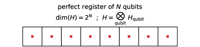
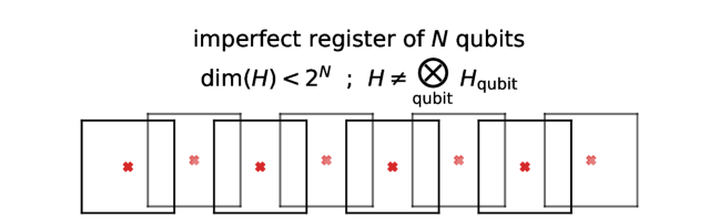
Figure 1: The upper sketch illustrates a perfect register of eight non-overlapping qubits. The Hilbert space of the entire register is the tensor product of the individual qubit Hilbert spaces. The lower sketch illustrates the situation when the total Hilbert space is strictly smaller than such a tensor product. In this case the qubits must be overlapping, by which we mean that the operator algebras defining the different qubits are not (anti-)commuting.

 

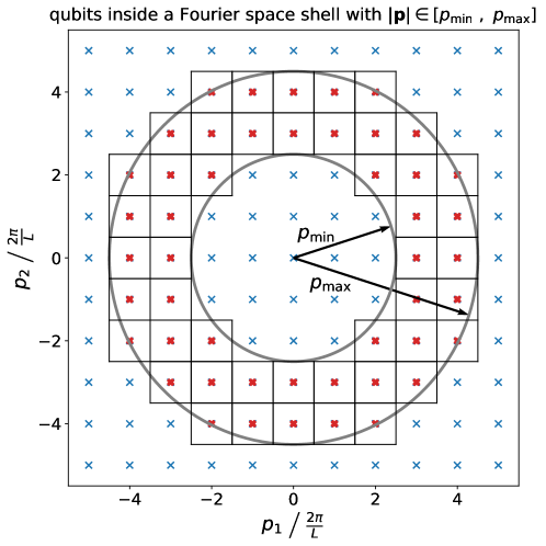
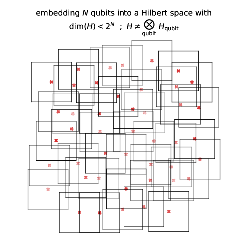
Figure 2: The ($c$-particle part of the) Weyl field can be decomposed into a collection of qubits, which are represented by points $\bm{p}$ in Fourier space (upper sketch). In 3 dimensions, the number of qubits in a small Fourier space shell $s$ (red crossed in upper sketch) scales as $k_{s}^{2}\Delta_{s}$ where $k_{s}$ is the radius and $\Delta_{s}$ is the width of the shell. We want to embed these qubits into a Hilbert space that is strictly smaller then the tensor product of the individual qubit Hilber spaces (cf. Figure 1) in order to achieve a holographic scaling of the effective degrees of freedom in our field.

We had already said that the Weyl field can be considered as a collection of qubits: one for each wave mode $\bm{p}$ in the particle sector and one for each wave mode $\bm{p}$ in the anti-particle sector (cf. Equation 3 as well as our sketch in Figure 2, which applies to either one of the two sectors). For a thin Fourier space shell $s$ of radius $k_{s}$ and width $\Delta_{s}$ the number density of modes $\bm{p}$ with $|\bm{p}|\in[k_{s}-\Delta_{s}/2,k_{s}+\Delta_{s}/2]$ per radius will scale as

$$\frac{N_{s}}{\Delta_{s}}\propto k_{s}^{2}\ ,$$ (7)

where $N_{s}$ is the total number of modes inside shell $s$. The above scaling is the Fourier space manifestation of the volume extensive scaling of QFT degrees of freedom. We will now squeeze the qubits present at these modes into a Hilbert space of dimension $2^{n_{s}}<2^{N_{s}}$ (cf. again Figure 2). To approximately achieve holography the radial number density of effective qubits in the shell should scale as [12]

$$\frac{n_{s}}{\Delta_{s}}\propto k_{s}\ ,$$ (8)

where $n_{s}$ is now the effective number of qubit degrees of freedom in shell $s$. At a first glance this procedure may seem infeasible, because for high momenta $k_{s}$ it may lead to a vast overpopulation of the physical Hilbert space with our unphysical qubits. But the authors of [43] have shown that - using the embedding procedure we outlined above - the physical Hilbert space can indeed be exponentially overcrowded with qubits (i.e. $n_{s}\sim\ln N_{s}$) while still keeping the operator norm of the anti-commutator of any pair of qubits smaller than some small parameter $\epsilon$.

Note that, in order to achieve holography, we don’t even need this exponential overcrowding. We only need polynomial overcrowding,

$$N_{s}\propto n_{s}^{2}\ .$$ (9)

This leads us to our first result: in Section 3 we show that in order to make the Weyl field obey a holographic scaling of the effective degrees of freedom and also satisfy the Bekenstein bound for the box of size $L$, we need to allow overlaps of the creation and annihilation operators for different field modes that are bounded by

$$|\{\hat{c}_{\bm{p}}^{\dagger},\hat{c}_{\bm{q}}\}|\,<\,\epsilon(k)\, \approx\,\sqrt{\frac{48\log\left(k_{s}L\right)}{\alpha\pi(k_{s}L)^{2}}}\,\frac{\Lambda_{\mathrm{UV}}}{\Lambda_{\mathrm{Planck}}}$$ (10)

$$\qquad\mathrm{for\ all}\ \ |\bm{p}|\approx k\approx|\bm{q}|,\ \bm{p}\neq\bm{q}\ .$$

Here $\alpha=\Delta_{s}/k_{s}$ is the relative width of the Fourier space shells, and we have explicitly allowed a UV-cutoff $\Lambda_{\mathrm{UV}}$ of our theory that is different from the Planck scale $\Lambda_{\mathrm{Planck}}$. The above result holds when $\hat{\psi}$ is the only quantum field in the Universe. In the presence of other fields, it changes to

$$\epsilon(k)\approx\sqrt{\frac{48\log\left(k_{s}L\right)}{\alpha\pi(k_{s}L)^{2}}}\,\sqrt{\frac{N_{\mathrm{dof,total}}}{N_{\mathrm{dof},\psi}}}\,\frac{\Lambda_{\mathrm{UV}}}{\Lambda_{\mathrm{Planck}}}\ ,$$ (11)

where $N_{\mathrm{dof,total}}$ are the total number of degrees of freedom present in the Universe and $N_{\mathrm{dof},\psi}$ are the degrees of freedom contributed by $\hat{\psi}$ .

We show the bound of Equation 11 for different values of the ratio $N_{\mathrm{dof},\psi}\ /\ N_{\mathrm{dof,total}}$ in Figure 3, fixing $\alpha=0.01$ and $\Lambda_{\mathrm{UV}}=\Lambda_{\mathrm{Planck}}$. Note that it is in fact decreasing with increasing wave number $k$ , i.e. at higher energies the overlap between different modes becomes more and more suppressed. At energies probed by the Large Hadron Collider it falls down to $\sim 10^{-43}$, indicating that any pair of Fourier modes in that regime behave as almost independent degrees of freedom (though see the end of Section 3.2 for a more nuanced discussion).

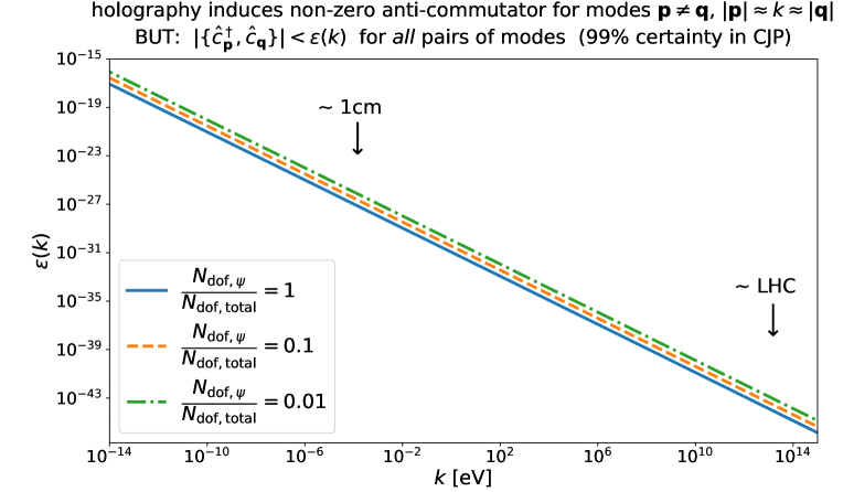
Figure 3: Bound on the anti-commutator $\{\hat{c}_{\mathbf{p}}^{\dagger},\hat{c}_{\mathbf{q}}\}$ induced for modes $\mathbf{p}\neq\mathbf{q}$, $|\mathbf{p}|\approx k\approx|\mathbf{q}|$, due to squeezing the degrees of freedom of our field into too small Hilbert spaces via the Chao-Johson-Lindenstrauss embedding (cf. Section 3). At energies probed by the Large Hadron Collider or at energies of everyday life (cf. small arrows) the bound is vastly smaller than the operator norms of $\hat{c}_{\mathbf{p}},\hat{c}_{\mathbf{p}}^{\dagger}$, indicating that any pair of Fourier modes behave as almost independent degrees of freedom. Different lines assume different ratios between the overall degrees of freedom of our field and the total degrees of freedom present in the Universe.

To investigate potential dynamical consequences of the non-vanishing Fourier mode overlaps, we consider a Hamiltonian for our field that takes the same form as for the standard non-overlapping Weyl field,

$$\hat{H} =\sum_{\bm{p}}|\bm{p}|\left\{\left(\hat{c}_{\bm{p}}^{\dagger}\hat{c}_{\bm{p}}-\frac{1}{2}\right)+\left(\hat{d}_{\bm{p}}^{\dagger}\hat{d}_{\bm{p}}-\frac{1}{2}\right)\right\}$$ (12)

$$\approx\sum_{\mathrm{shell}\ s}k_{s}\sum_{\bm{p}\in s}\left\{\left(\hat{c}_{\bm{p}}^{\dagger}\hat{c}_{\bm{p}}-\frac{1}{2}\right)+\left(\hat{d}_{\bm{p}}^{\dagger}\hat{d}_{\bm{p}}-\frac{1}{2}\right)\right\}\ ,$$

where in the second line we made explicit our decomposition of Fourier space into a set of shells. Within each shell the occupation number operators $\hat{N}_{\bm{p}}=\hat{c}_{\bm{p}}^{\dagger}\hat{c}_{\bm{p}}$, $\hat{N}_{\bm{q}}=\hat{c}_{\bm{q}}^{\dagger}\hat{c}_{\bm{q}}$ of different Fourier modes $\bm{p}$ and $\bm{q}$ will not commute anymore. This also means that $[\hat{H},\hat{N}_{\bm{p}}]\neq 0$ and the occupation number in a given Fourier mode is not conserved, despite Equation 12 formally looking like the free field Hamiltonian. To determine the severity of this effect we first define plane wave states in our theory through the following steps:

• consider the states $\ket{\psi(t)}$ which at an initial time $t_{0}$ start in the eigenspace of $\hat{N}_{\bm{p}}$ with eigenvalue $+1\,$, i.e. $\hat{N}_{\bm{p}}\ket{\psi(t_{0})}=+\ket{\psi(t_{0})}$;

• in this subspace, find the states that minimize $\left|\left[\frac{\mathrm{d}^{2}}{\mathrm{d}t^{2}}\bra{\psi(t)}\hat{N}_{\bm{p}}\ket{\psi(t)}\right]_{t=t_{0}}\right|$ ;

• this condition is still satisfied by an entire subspace of states, so our final selection step is to choose the candidate state that initially has the lowest energy expectation value $\bra{\psi(t_{0})}\hat{H}\ket{\psi(t_{0})}$ .

In the following we will use the notation $\ket{\bm{p}}\equiv\ket{\psi(t_{0})}\,$, where $\ket{\psi(t)}$ is chosen as explained above, and we will consider $\ket{\bm{p}}$ as the closest equivalent our theory has to the standard plane wave state $\hat{c}_{\bm{p}}^{\dagger}\ket{0}$ for the non-overlapping Weyl field. In the standard theory, plane wave states would be eigenstates of the Hamiltonian operator and thus have a trivial time evolution. In our holographic version of the Weyl field this is not the case anymore. Operators $\hat{N}_{\bm{p}}$ and $\hat{N}_{\bm{q}}$ for different modes $\bm{p},\bm{q}$ do not commute any longer, and thus the Hamiltonian (which is a sum over all the different occupation number operators) does not commute with any of the $\hat{N}_{\bm{p}}$ either. As a consequence, time evolution will move the states $\ket{\bm{p}}$ out of the $+1$-eigenspace of $\hat{N}_{\bm{p}}\,$. Note however that we have assumed different Fourier space shells to be non-overlapping, so the initial probability amplitude in $\ket{\bm{p}}$ will only be re-distributed with the shell that contains $\bm{p}\,$. Since in our fiducial construction the overlaps between different modes is independent of their relative direction, we interpret this modified time evolution as an isotropic scrambling of plane waves within their Fourier space shells. This indicates a breaking of Lorentz symmetry (in particular, of momentum conservation), and we discuss implications of that in Section 3.4.

To quantify the severity of the scrambling effect, we estimate a characteristic lifetime of plane waves as

$$\frac{1}{T_{\mathrm{scramble}}^{2}}=-\mathbb{E}\left\{\frac{\mathrm{d}^{2}}{\mathrm{d}t^{2}}\bra{\bm{p}}\hat{N}_{\mathbf{p}}\ket{\bm{p}}\right\}\ ,$$ (13)

where the expectation value $\mathbb{E}\{\cdot\}$ is taken with respect to the random vectors that are used in the CRSV-embedding to construct representations of the different field modes (cf. Section 3). In C.2 we demonstrate analytically that the following relation between $T_{\mathrm{scramble}}$ and the momentum $|\bm{p}|$ holds in the large-$n_{s}$ limit (cf. more details also in Section 4):

$$\frac{\mathrm{d}^{2}}{\mathrm{d}t^{2}}\bra{\bm{p}}\hat{N}_{\bm{p}}\ket{\bm{p}}\propto\frac{|\bm{p}|^{2}}{|\bm{p}|L}$$ (14)

$$\Rightarrow T_{\mathrm{scramble}}\propto\sqrt{\frac{L}{|\bm{p}|}}\ .$$ (15)

The exact amplitude of this scaling depends on the values of different parameters of our construction, and in particular on ultraviolet cutoff $k_{\mathrm{UV}}\,$: choosing a higher $k_{\mathrm{UV}}$ requires larger mode overlaps in order to still satisfy the cosmic Bekenstein bound, which in turn leads to a stronger scrambling. Figuratively speaking, the mode overlaps generate a cosmic fog and that fog has to become thicker when $k_{\mathrm{UV}}$ is increased, i.e. when more modes are allowed to exist. In Figure 4 we illustrate the impact of choosing different UV-cuts, fixing the other parameters to fiducial values detailed in Sections 3.2 and 3.3. In that figure we also indicate the typical energies and travel distances of neutrinos created by a number of known and resolved sources (see also Table 1 for a summary; we assume that the neutrino dispersion relation is still close to light-like in order to translate lifetimes to distances). We provide a more detailed discussion of these results in Section 4, but the highly energetic neutrino emission observed from blazar TXS 0506+056 requires $k_{\mathrm{UV}}<470\,k_{\mathrm{LHC}}\,$, where we take $k_{\mathrm{LHC}}=14\,$TeV. So electroweak theory should be modified only a few orders of magnitude above modern particle physics experiments. In Section 4.3 we argue that this is still consistent with current measurements of the cosmic neutrino spectrum by IceCube (cf. Figure 7 in that section). The breakdown of our effective theory beyond the energy $k_{\mathrm{UV}}$ should happen either as a sharp cutoff or as a transition to super-holographic mode overlaps, because any modes present beyond $k_{\mathrm{UV}}$ need to be squeezed into a very small part of the total Hilbert space in order to still satisfy the Bekenstein bound.

Figure 4: Lifetimes of plane waves in the holographic Weyl field depend on the UV-cut of our theory. We display the corresponding free path as a function of plane wave energy according to our calculations in C.2 (see also Section 4.2) for $k_{\mathrm{UV}}=k_{\mathrm{Planck}}$ (blue, dotted line), for $k_{\mathrm{UV}}=10^{-3}\,k_{\mathrm{Planck}}$ (orange, dash-dotted line), and for $k_{\mathrm{UV}}=470\,k_{\mathrm{LHC}}$ (green, dashed line). All of these lines assume a static Universe, a light-like dispersion relation and that our holographic field makes up 1% of the total effective degrees of freedom present in the Universe (cf. Section 3.3 for a discussion of that choice). We also indicate the energies and path lengths for a number of known and resolved sources of neutrino emission - cf. Table 1 for more details. To explain how all of these events could have been observed, we need to assume a break down of neutrino EFT at $\lesssim$ 500 times the collision energies reached at the LHC.

Apart from the behaviour of plane waves, it is also possible to understand the dynamics of our field more generally. In C.1 we use results from random matrix theory to derive that the set of eigenvalues of the Hamiltonian in each individual shell of Equation 12 is given by

$$\{\lambda\} =\left\{\left.\frac{k_{s}}{2}\sum_{i=1}^{n_{s}}\lambda_{i}s_{i}\ \right|\ \{s_{i}\}\in[-1,+1]^{n_{s}}\right\}\ ,$$ (16)

where $\lambda_{i}$ are the positive eigenvalues of a generalised Wigner matrix. Using a rigidity property for the eigenvalues of Wiger matrices derived by [44] the $i$th of these eigenvalues will be given with high accuracy by the $i/n_{s}$-quantile of a Wigner semi-circle distribution. In particular we are able to derive the vacuum energy in a Fourier space shell of width $\Delta_{s}$ and radius $k_{s}$ as

$$E_{\min,s} \approx-\frac{N_{s}k_{s}}{2}\cdot\left(\frac{8}{3\pi}\sqrt{\frac{\displaystyle n_{s}}{\displaystyle N_{s}}}\right)\ .$$ (17)

In Figure 5 we have used simulated realisations of overlapping qubits to show that this result is accurate already for quite low numbers of field modes. At energies (and hence mode numbers) relevant for high-energy physics, it represents a strong suppression with respect to the non-overlapping Weyl field, whose vacuum energy in each shell would simply be $-N_{s}k_{s}/2$. When choosing $\Lambda_{\mathrm{UV}}=\Lambda_{\mathrm{Planck}}$ the total vacuum energy of the field is lowered by a factor of $\sim 10^{-30}$ (which is however not enough to alleviate the cosmological constant problem).

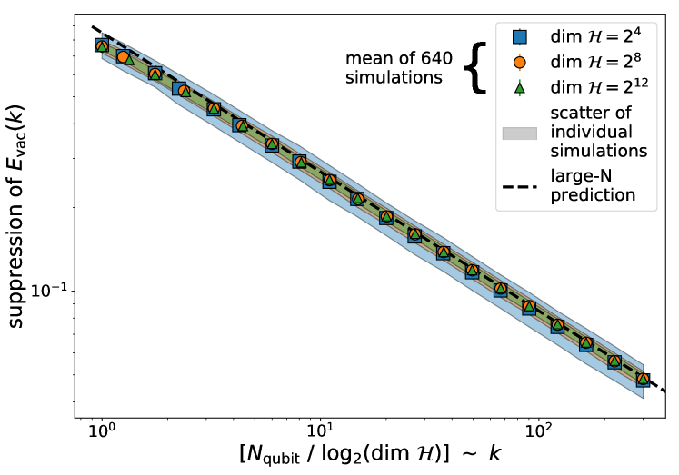
Figure 5: Suppression of minimum eigenvalue of the Hamiltonian (compared to the case of non-overlapping degrees of freedom) in a Fourier space shell $s$ of our holographic Weyl field as a function of its overcrowding $N_{s}/n_{s}$ ($=N_{\mathrm{qubit}}/\log_{2}(\dim\mathcal{H})$ in the figure label). Note that $N_{s}\propto k_{s}^{2}\Delta_{s}$ and $n_{s}\propto k_{s}\Delta_{s}$, where $\Delta_{s}$ is the width of the shell and $k_{s}$ its radius. Thus, $N_{s}/n_{s}\propto k_{s}$, i.e. the $x$-axis of the figure is proportional to shell radius. The different symbols represent measurements of vacuum energy suppression in simulated realisations of the Fourier space shells for $n_{s}=4,8,12$. Overall $640$ independent realisations of those simulations have been averaged to obtain these measurements. The transparent bands indicate the standard deviation of the individual realisations. The dashed line displays our theoretical prediction for the suppression of vacuum energy, as derived in C. Note that due to numerical limitations we were only able to simulate very low dimensional shells. Our theoretical prediction will become even more precise at higher values of $n_{s}$ and $N_{s}$ because it describes an asymptotic, high-dimensional limit.

Neutrino sources	characteristic energy scale	travel distance $d_{\mathrm{source}}$	UV-scale where Fermion EFT must break down in order to ensure $d_{\mathrm{source}}<T_{\mathrm{scramble}}/c$	vacuum energy suppression          (due to holography & UV-cut)
Atlas detector	$\lesssim$ 14 TeV	50 m	$1.04\,k_{\mathrm{Planck}}\,=\,9.1\cdot 10^{14}\,k_{\mathrm{LHC}}$	$1.4\cdot 10^{-31}$                (for $k_{\mathrm{UV}}=k_{\mathrm{Planck}}$)
CERN $\rightarrow\$ Gran Sasso ([45])	$\sim$ 30 GeV	731 km	$4.0\cdot 10^{-2}\,k_{\mathrm{Planck}}\,=\,3.5\cdot 10^{13}\,k_{\mathrm{LHC}}$	$1.9\cdot 10^{-36}$
Solar       (e.g. [46])	$<$ 18 MeV	$1.5\cdot 10^{12}$ m	$1.8\cdot 10^{-4}\,k_{\mathrm{Planck}}\,=\,1.6\cdot 10^{11}\,k_{\mathrm{LHC}}$	$1.1\cdot 10^{-44}$
SN  1987A          ([47, 48])	$\lesssim$ 20 MeV	$1.6\cdot 10^{18}$ m	$1.7\cdot 10^{-7}\,k_{\mathrm{Planck}}\,=\,1.5\cdot 10^{8}\,k_{\mathrm{LHC}}$	$2.9\cdot 10^{-55}$
TXS 0506+056 ([49])	$\sim$ 290 TeV	$4.1\cdot 10^{25}$ m $\approx 1.3$ Gpc	$5.4\cdot 10^{-13}\,k_{\mathrm{Planck}}\,=\,4.7\cdot 10^{2}\,k_{\mathrm{LHC}}$	$1.7\cdot 10^{-74}$

Table 1: Known and resolved sources of neutrinos, their typical energies and their travel distances. In order for the travel time of these particles to be shorter than the plane wave scrambling time of our holographic construction, we need to impose UV cutoffs that are significantly below the Planck scale (but still safely above energy scales probed at the LHC; cf. 4th column). Holography and the UV cutoffs combine to suppress vacuum energy density significantly compared to a standard Fermion with $k_{\mathrm{UV}}=k_{\mathrm{Planck}}$ (but not enough to solve the cosmological constant problem; cf. 5th column). The table employs our fiducial assumption that about $1\%$ of the Universes degrees of freedom are contributed by our holographic Fermion. Whether this is a realistic assumption depends on the degree to which different quantum fields overlap with each other (cf. our discussion in Section 3.3).

Finally, in Section 5 we investigate the impact of the overlapping Fourier modes on the real space propagator $\{i\psi_{\alpha}(\bm{x})^{\dagger},\psi_{\beta}(\bm{y})\}$ . After tracing out the spin degree of freedom labelled by $\alpha,\beta$ we obtain

$$\sum_{\alpha}\{i\psi_{\alpha}(\bm{x})^{\dagger},\psi_{\alpha}(\bm{y})\}=2i\delta_{D}(\bm{x}-\bm{y})+2iC(\bm{x},\bm{y})\ .$$ (18)

The first term on the right hand side of Equation 18 is the result one would obtain for the standard Weyl field and the second term is a correction induced by the mode overlap. Since we squeeze the degrees of freedom of our field into the true, physical Hilbert space of the field via a stochastic procedure, the function $C(\bm{x},\bm{y})$ is also stochastic. It vanishes on average, $\mathbb{E}[C(\bm{x},\bm{y})]=0$  , but it fluctuates with an amplitude

$$\sqrt{\mathbb{E}\left[|C(\bm{x},\bm{y})|^{2}\right]} =\frac{1}{\sqrt{128\pi^{5}}}\frac{\Lambda_{\mathrm{UV}}^{2}}{L}\ ,$$ (19)

where $L$ is again the IR scale corresponding to the size of the box to which we confine our field, and $\Lambda_{\mathrm{UV}}$ is a UV cutoff. Note that the amplitude of the correction term is in fact independent of $\bm{x}$, $\bm{y}$ and in particular their distance. So, within our construction, a holographic scaling of the effective field degrees of freedom manifests itself as a stochastic, long-range contribution to the field propagator. In particular, the correction can be interpreted as a source of non-locality because the field and its conjugate momentum do not anti-commute at non-zero, equal-time distances.

Since the correction term $2iC(\bm{x},\bm{y})$ in Equation 18 has a scale independent amplitude, it is tempting to assume that the standard term $2i\delta_{D}(\bm{x}-\bm{y})$ will always dominate the propagator at sufficiently small distances $\bm{x}-\bm{y}$ . To make this assumption more precise, and in order to test it, we smooth our field with a Gaussian test function of width $R$ (standard deviation). The resulting smoothed field $\hat{\psi}_{R}$ has the propagator

$$\sum_{\alpha}\{i\psi_{R,\alpha}(\bm{x})^{\dagger},\psi_{R,\alpha}(\bm{y})\}\ =\ 2iC_{R}(\bm{x},\bm{y})+\frac{2i}{\sqrt{(4\pi)^{3}R^{6}}}\ e^{-\frac{1}{4R^{2}}|\bm{x}-\bm{y}|^{2}}$$ (20)

$$\equiv\ 2iD_{R}(\bm{x},\bm{y})\ ,$$

where for simplicity we have again taken the trace over spin degrees of freedom, and where $C_{R}(\bm{x},\bm{y})$ is an appropriately smoothed version of $C(\bm{x},\bm{y})$. We can then compare the average fluctuation of the long-range propagator (which is dominated by $C_{R}(\bm{x},\bm{y})$) to the average local propagator (which is given by the standard local propagator because $\mathbb{E}[C_{R}]=0$). In particular, we consider the ratio of these two and in Section 5 we obtain

$$\frac{\mathbb{E}\left[|C_{R}(\bm{x},\bm{y})|^{2}\right]}{\mathbb{E}[D_{R}(\bm{x},\bm{x})]\ \mathbb{E}[D_{R}(\bm{y},\bm{y})]}\ =\ \frac{N_{\mathrm{dof,total}}}{N_{\mathrm{dof},\psi}}\left(\frac{2R}{\pi L}\right)^{2}\ .$$ (21)

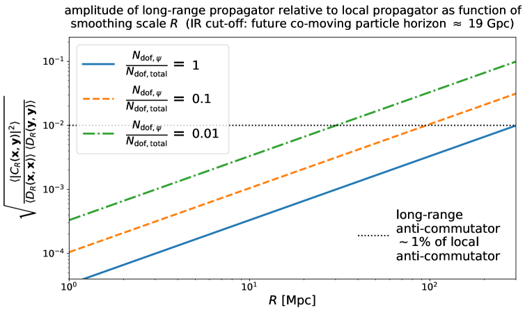
Figure 8: The overlap of Fourier modes generates a non-zero propagator at large equal-time distances in real space. We show the average amplitude of this long-range anti-commutator relative to the local anti-commutator when smoothing the field by different scales $R$ . Even for cosmological smoothing scales ($R\,\sim 30$ Mpc) this ratio remains at a level of $\sim 1\%$ (cf. Section 5).

We display the square root of this ratio in the lower panel of Figure 8 for different values of the ratio $N_{\mathrm{dof},\psi}/N_{\mathrm{dof,total}}$ . Even for cosmologically large smoothing scales ($R\,\sim 30$ Mpc) the typical amplitude of the long-range propagator remains at a level of $\sim 1\%$ of the local anti-commutator. So the non-locality induced by our holographic scaling of the effective field degrees of freedom seems to become significant only on very large scales. In a sense, this is just the real space equivalent of our result regarding the mode anti-commutators $\{\hat{c}_{\mathbf{p}}^{\dagger},\hat{c}_{\mathbf{q}}\}$ from Figure 3.

The rest of this paper is structured as follows. In Section 2 we review basics of the Weyl field and how to decompose it into a set of qubits. Section 3 then introduces modifications to make the degrees of freedom of this field obey an approximate area law scaling. We study the dynamics of our holographic Weyl field in Section 4. In particular, results about its energy spectrum are presented in Section 4.1 and we discuss our definition of plane waves and their lifetime in Section 4.2. Section 5 investigates the real space anti-commutator of our field, while Section 6 repeats some of our analysis for two possible modifications of our fiducial construction. In Section 7 we put our construction into the context of quantum mereology and discuss why classical stochasticity like the one present in our qubit overlaps is likely to arise in a dynamical emergence of classical degrees of freedom from an abstract quantum theory. Finally, Section 8 summarises our paper and provides an outlook.

Note that many of our technical results are derived in our appendices (in particular C) and only quoted in the main text.

2 The Weyl field as a collection of qubits

For the sake of simplicity we consider a Weyl fermion, which corresponds to one of the two helicity sectors of a massless Dirac fermion. This section serves as a reminder of the Weyl formalism. We also make explicit in which sense the Weyl field can be decomposed into a collection of qubits. In Section 3 we will use this decomposition to define a modified version of the Weyl field, in which certain degrees of freedom are overlapping.

2.1 Weyl field basics

The (left-handed) Weyl spinor is a two-component field $\psi$ with the Lagrangian

$$\mathcal{L}=i\psi^{\dagger}\sigma^{\mu}\partial_{\mu}\psi\ ,$$ (22)

where $\sigma^{0}\equiv\mathbf{1}$ and $\sigma^{i}$ are e.g. the Pauli matrices (we are following here the notation of [50, 51]). The above Lagrangian leads to the equations of motion

$$\sigma^{\mu}\partial_{\mu}\psi=0\ .$$ (23)

A general solution to these equations can be expressed as

$$\psi(\bm{x},t) =\int\frac{\mathrm{d}^{3}p}{(2\pi)^{3}E_{p}}\ \left\{a_{\bm{p}}(t)u(\bm{p})\ e^{i\bm{p}\bm{x}}+b_{\bm{p}}^{*}(t)u(\bm{p})\ e^{-i\bm{p}\bm{x}}\right\}\ ,$$ (24)

where the time evolution of the coefficients $a_{\bm{p}}$ and $b_{\bm{p}}^{*}$ is given by

$$a_{\bm{p}}(t)=a_{\bm{p},0}\ e^{-iE_{p}t}\ ,\ b_{\bm{p}}(t)^{*}=b_{\bm{p},0}^{*}\ e^{iE_{p}t}$$ (25)

with $E_{p}\equiv|\bm{p}|$, and where $u(\bm{p})$ are eigenvectors of the matrix $\sigma^{j}p_{j}$ with eigenvalues $+E_{p}$ ,

$$\sigma^{j}p_{j}\cdot u(\bm{p})=+E_{p}\ u(\bm{p})\ .$$ (26)

Note that in the following we will keep the time dependence of $a_{\bm{p}}$ and $b_{\bm{p}}^{*}$ implicit in our notation. The reason is that this dependence will deviate from Equation 25 once we consider overlapping degrees of freedom.

Normalising the $u(\bm{p})$ such that

$$u(\bm{p})^{\dagger}\cdot u(\bm{p})=E_{p}$$ (27)

ensures that they are orthogonal wrt. the Lorentz invariant momentum space measure

$$\mathrm{d}\tilde{p}:=\frac{\mathrm{d}^{3}p}{(2\pi)^{3}\ E_{p}}\ .$$ (28)

Up to an irrelevant phase factor we can e.g. choose $u(\bm{p})$ as [51]

$$u(\bm{p})=\sqrt{E_{p}}\pmatrix{e^{-i\phi}\sin\frac{\theta}{2}\cr\cos\frac{\theta}{2}}\ ,$$ (29)

where $\bm{p}=(p\sin\theta\cos\phi,p\sin\theta\sin\phi,p\cos\theta)^{T}$ .

In the quantum version of the above field theory we consider the operator valued field

$$\hat{\psi}(\bm{x},t) =\int\mathrm{d}\tilde{p}\ \left\{\hat{a}_{\bm{p}}(t)u(\bm{p})\ e^{i\bm{p}\bm{x}}+\hat{b}_{\bm{p}}(t)^{\dagger}u(\bm{p})\ e^{-i\bm{p}\bm{x}}\right\}\ ,$$ (30)

where the operator $\hat{b}_{\bm{p}}^{\dagger}$ can be thought of as creating an anti-spinor of momentum $\bm{p}$ while $\hat{a}_{\bm{p}}$ is destroying a spinor with momentum $\bm{p}$. At equal times these operators satisfy the anti-commutation relations

$$0=\{\hat{a}_{\bm{p}},\hat{a}_{\bm{q}}\}=\{\hat{b}_{\bm{p}},\hat{b}_{\bm{q}}\}=\{\hat{a}_{\bm{p}},\hat{b}_{\bm{q}}\}=\{\hat{a}_{\bm{p}},\hat{b}_{\bm{q}}^{\dagger}\}$$ (31)

$$\{\hat{a}_{\bm{p}},\hat{a}_{\bm{q}}^{\dagger}\}=\{\hat{b}_{\bm{p}},\hat{b}_{\bm{q}}^{\dagger}\}=(2\pi)^{3}E_{p}\ \delta_{D}(\bm{p}-\bm{q})\ .$$ (32)

This ensures that the field operators satisfy the equal-time anti-commutation relation

$$\{\hat{\psi}(\bm{x}),i\hat{\psi}(\bm{y})^{\dagger}\}$$ (33)

$$\ \ \ =i\int\mathrm{d}\tilde{p}\mathrm{d}\tilde{q}\ \left[\{\hat{a}_{\bm{p}},a_{\bm{q}}^{\dagger}\}\ u(\bm{p})u(\bm{q})^{\dagger}+\{\hat{b}_{-\bm{p}}^{\dagger},b_{-\bm{q}}\}\ u(-\bm{p})u(-\bm{q})^{\dagger}\right]e^{i\bm{p}\bm{x}-i\bm{q}\bm{y}}$$

$$\ \ \ =i\int\frac{\mathrm{d}^{3}p}{(2\pi)^{3}E_{p}}\ \left[u(\bm{p})u(\bm{p})^{\dagger}+u(-\bm{p})u(-\bm{p})^{\dagger}\right]e^{i\bm{p}(\bm{x}-\bm{y})}$$

$$\ \ \ =i\ \mathbf{1}_{\mathrm{2D}}\ \delta_{D}(\bm{x}-\bm{y})\ ,$$ (34)

as is needed because $i\hat{\psi}^{\dagger}$ is the conjugate momentum of the field $\hat{\psi}$ .

2.2 Decomposition into qubits

To make it explicit that the above field can be considered as a collection of qubits, let us constrict $\psi(\bm{x})$ to a box of finite size $L$ . This means that we have to perform the substitutions

$$\mathrm{d}^{2}p\rightarrow\frac{(2\pi)^{3}}{L^{3}}\ ,\ \delta_{D}(\bm{p}-\bm{q})\rightarrow\frac{L^{3}}{(2\pi)^{3}}\delta_{\bm{p},\bm{q}}\ ,$$ (35)

and that integrals over momenta will be replaced by sums over the discrete grid $\bm{p}\in\{\ 2\pi/L(n_{1},n_{2},n_{3})\ |\ n_{i}\in\mathbb{Z}\ \}$ . For convenience, we will also consider redefined mode operators

$$\hat{c}_{\bm{p}}=\frac{\hat{a}_{\bm{p}}}{(E_{p}V)^{\frac{1}{2}}}\ ,\ \hat{d}_{\bm{p}}=\frac{\hat{b}_{\bm{p}}}{(E_{p}V)^{\frac{1}{2}}}\ ,$$ (36)

such that the new operators satisfy the anti-commutation relations

$$0=\{\hat{c}_{\bm{p}},\hat{c}_{\bm{q}}\}=\{\hat{d}_{\bm{p}},\hat{d}_{\bm{q}}\}=\{\hat{c}_{\bm{p}},\hat{d}_{\bm{q}}\}=\{\hat{c}_{\bm{p}},\hat{d}_{\bm{q}}^{\dagger}\}$$ (37)

$$\{\hat{c}_{\bm{p}},\hat{c}_{\bm{q}}^{\dagger}\}=\{\hat{d}_{\bm{p}},\hat{d}_{\bm{q}}^{\dagger}\}=\delta_{\bm{p},\bm{q}}\ .$$ (38)

Our field can now be decomposed in terms of these operators as

$$\hat{\psi}(\bm{x},t)=\sum_{\bm{p}}\frac{1}{(E_{p}V)^{\frac{1}{2}}}\left\{\hat{c}_{\bm{p}}(t)\ u(\bm{p})\ e^{i\bm{p}\bm{x}}+\hat{d}_{\bm{p}}(t)^{\dagger}\ u(\bm{p})\ e^{-i\bm{p}\bm{x}}\right\}\ .$$ (39)

Usually, each of the grid points $\bm{p}$ in the above sum represents a 4-dimensional Hilbert space factor

$$\mathcal{H}_{\bm{p}}=\mathcal{H}_{\bm{p}}^{c}\otimes^{\mathrm{JW}}\mathcal{H}_{\bm{p}}^{d}$$ (40)

and the total Hilbert space is the tensor product over all these factors,

$$\mathcal{H}=\bigotimes_{\bm{p}}^{\mathrm{JW}}\mathcal{H}_{\bm{p}}\ ,$$ (41)

where the superscript JW again indicates that operators in the individual Hilbert spaces need to be embedded into the product space via Jordan-Wigner-factors (cf. D) in order for them to anti-commute (as opposed to commute). The $\hat{c}_{\bm{p}}$, $\hat{d}_{\bm{p}}$ and their Hermitian conjugates act non-trivially only on the factors $\mathcal{H}_{\bm{p}}^{c}$ and $\mathcal{H}_{\bm{p}}^{d}$ respectively. On the factor $\mathcal{H}_{\bm{p}}^{c}$ (and similarly for $\mathcal{H}_{\bm{p}}^{d}$) we can define

$$\hat{\sigma}_{x,\bm{p}}^{c} =\hat{c}_{\bm{p}}+\hat{c}_{\bm{p}}^{\dagger}$$ (42)

$$\hat{\sigma}_{y,\bm{p}}^{c} =i\left(\hat{c}_{\bm{p}}-\hat{c}_{\bm{p}}^{\dagger}\right)$$ (43)

$$\hat{\sigma}_{z,\bm{p}}^{c} =-i\hat{\sigma}_{x,\bm{p}}^{c}\hat{\sigma}_{y,\bm{p}}^{c}=2\hat{c}_{\bm{p}}^{\dagger}\hat{c}_{\bm{p}}-1\ .$$ (44)

These operators constitute a Pauli algebra on the qubit Hilbert space $\mathcal{H}_{\bm{p}}^{c}$ . Note however, that the labels $x,y,z$ are simply notation, and not meant to indicate directions in physical space. The Hamiltonian of the field can be expressed in terms of these operators as

$$\hat{H} =\sum_{\bm{p}}E_{p}\left\{\left(\hat{c}_{\bm{p}}^{\dagger}\hat{c}_{\bm{p}}-\frac{1}{2}\right)+\left(\hat{d}_{\bm{p}}^{\dagger}\hat{d}_{\bm{p}}-\frac{1}{2}\right)\right\}$$ (45)

$$=\sum_{\bm{p}}\frac{E_{p}}{2}\left\{\hat{\sigma}_{z,\bm{p}}^{c}+\hat{\sigma}_{z,\bm{p}}^{d}\right\}\ .$$

So our field behaves like a set of non-interacting spins in a $\bm{p}$-dependent magnetic field.

3 Fermion field with overlapping qubits

3.1 Chao-Reichert-Sutherland-Vidick embedding

We will now use the scheme of [24] for embedding $N$ qubits into an Hilbert space of dimension $2^{n}<2^{N}$ (Chao-Reichert-Sutherland-Vidick embedding, or CRSV-embedding for the rest of this paper) to create a version of the Weyl field whose effective degrees of freedom approximately follow an area law scaling. To describe our approach we will focus on the particle part of the field (the anti-particle part can be treated analogously). We start by covering the entirety of Fourier space with adjacent but non-overlapping shells $\{s\}$ (cf. our sketch in Figure 2), and we introduce the following notation.

• $k_{s}\,,\ \Delta_{s}$ :

  the central radius and width of Fourier space shell $s$.

• $N_{s}$ :

  number of qubits inside Fourier space shell $s$  (i.e. the number of momenta $\bm{p}\in s$).

• $n_{s}$ :

  logarithm (to the base $2$) of the dimension into which the $N_{s}$ will be embedded.

For our regular grid in Fourier space we expect

$$N_{s}\ \approx\ 4\pi k_{s}^{2}\Delta_{s}\ \bigg{/}\ \frac{(2\pi)^{3}}{L^{3}}\ ,$$ (46)

where $k_{s}$ is the central radius of shell $s$. The scaling $N_{s}\propto k_{s}^{2}\Delta_{s}$ indicates a volume scaling of the independent degrees of freedom, but we will squeeze the qubits of shell $s$ into a Hilbert space that is too small for them to be independent. In particular we would like to obtain an area-scaling of the effective degrees of freedom, such that [12]

$$\frac{n_{s}}{N_{s}}\propto\frac{k_{s}\Delta_{s}}{k_{s}^{2}\Delta_{s}}=\frac{1}{k_{s}}\ .$$ (47)

This will be achieved if

$$n_{s}=B\cdot 2\pi k_{s}\Delta_{s}\ \bigg{/}\ \frac{(2\pi)^{2}}{L^{2}}\ ,$$ (48)

where $B$ is some constant, and where the factors of $L/2\pi$ are just for later convenience. Along the lines of [24] we will now proceed as follows:

• For each shell $s$ we choose a $2^{n_{s}}$-dimensional matrix representation of the Clifford algebra with generators $\bm{C}_{1}$, …, $\bm{C}_{2n_{s}}$ .

• In the space $\mathbb{R}^{2n_{s}}$ , we draw $2N_{s}$ random vectors from a standard normal distribution.

• We collect these vectors into $N_{s}$ pairs (corresponding to the $N_{s}$ momenta $\bm{p}$ in the Fourier space shell $s$), and choose orthonormal bases $\{\ket{v_{\bm{p}}},\ket{w_{\bm{p}}}\}$ for the $N_{s}$ 2-dimensional subspaces spanned by these vector pairs.

• For some orthonormal basis $\{\ket{e_{j}}\}$ of $\mathbb{R}^{2n_{s}}$, we define

  $$\bm{\sigma}_{x,\bm{p}}^{c}\equiv\sum_{j=1}^{2n}\braket{e_{j}}{v_{\bm{p}}}\bm{C}_{j}\ \ ,\ \ \bm{\sigma}_{y,\bm{p}}^{c}\equiv\sum_{j=1}^{2n}\braket{e_{j}}{w_{\bm{p}}}\bm{C}_{j}\ \ ,\ \ \bm{\sigma}_{z,\bm{p}}^{c} =-i\bm{\sigma}_{x,\bm{p}}^{c}\bm{\sigma}_{y,\bm{p}}^{c}\ ,$$

  and we set

  $$\bm{c}_{\bm{p}}=\frac{1}{2}\left(\bm{\sigma}_{x,\bm{p}}^{c}+i\bm{\sigma}_{y,\bm{p}}^{c}\right)\ .$$ (50)

  (Note that this is slightly different from how [24] had originally defined their embedding. The reason for this is that we want the creation and annihilation operators for different modes $\bm{p}_{1},\,\bm{p}_{2}$ to approximately anti-commute, while [24] wanted operators on different qubits to approximately commute.)

• The matrices $\bm{c}_{\bm{p}}^{\dagger}$ and $\bm{c}_{\bm{p}}$ can serve as creation and annihilation operators in the Hilbert space $\mathcal{H}_{s}^{c}$ corresponding to shell $s$. In principle we now only have to stitch together different shells to obtain the creation and annihilation operators $\hat{c}_{\bm{p}}^{\dagger}$ and $\hat{c}_{\bm{p}}$ in the whole Hilbert space

  $$\mathcal{H}^{c}=\bigotimes_{s}\mathcal{H}_{s}^{c}\ .$$ (51)

  A naive attempt to do so would be to define $\hat{c}_{\bm{p}}=\left(\bigotimes_{\bm{p}\notin s}\mathbf{1}_{s}\right)\otimes\bm{c}_{\bm{p}}$ , i.e. to consider a tensor product of the operator $\bm{c}_{\bm{p}}$ (which is defined on the Hilbert space of the shell that contains $\bm{p}$) with the unit operators in all shells that do now contain $\bm{p}$. This naive approach would not work, because we need operators $\hat{c}_{\bm{p}}$ and $\hat{c}_{\bm{q}}$ that live on different shells to be anti-commuting (instead of commuting).

  To achieve anti-commutation between different shells, we need to insert the appropriate Jordan-Wigner strings into the above, naive construction. We sketch in D how this can be done in practice. But the details of this do not matter in the following, since they do not impact any anti-commutators that are relevant to our calculations.

• Finally, we duplicate the above construction for the $d$-particles and build the full Hilbert space as the tensor product of the spaces of particles and anti-particles (again, using an appropriate Jordan-Wigner construction to ensure anti-commutation between $c$- and $d$-operators).

Within the above construction the anti-commutator between the operators $\hat{c}_{\bm{p}}^{\dagger}$ and $\hat{c}_{\bm{q}}$, where $\bm{p}$ and $\bm{q}$ are in the same Fourier space shell $s$, becomes

$$\{\hat{c}_{\bm{p}}^{\dagger},\hat{c}_{\bm{q}}\} =\frac{1}{4}\sum_{jl}\braket{e_{j}}{v_{\bm{p}}-iw_{\bm{p}}}\braket{e_{l}}{v_{\bm{q}}+iw_{\bm{q}}}\{\bm{C}_{j},\bm{C}_{l}\}$$ (52)

$$=\frac{\braket{v_{\bm{p}}}{v_{\bm{q}}}+\braket{w_{\bm{p}}}{w_{\bm{q}}}+i\braket{v_{\bm{p}}}{w_{\bm{q}}}-i\braket{w_{\bm{p}}}{v_{\bm{q}}}}{2}$$

$$\equiv\frac{\braket{z_{\bm{p}}}{z_{\bm{q}}}}{2}\ ,$$

where in the last line we have introduced the complex vectors $\ket{z_{\bm{p}}}=\ket{v_{\bm{p}}}+i\ket{w_{\bm{p}}}$ . Note that in general $\braket{z_{\bm{p}}}{z_{\bm{q}}}\neq 0$ for $\bm{p}\neq\bm{q}$, because the vectors $\ket{v_{\bm{p}}},\ket{w_{\bm{p}}}$ are more numerous than their dimension (and because we chose these vector pairs randomly). At the same time, it is easy to check that $\braket{z_{\bm{p}}}{z_{\bm{p}}}=2$ and hence $\{\hat{c}_{\bm{p}}^{\dagger},\hat{c}_{\bm{p}}\}=1$.

The vectors $\ket{v_{\bm{p}}},\ket{w_{\bm{p}}}$ that are used in the above embedding procedure are chosen at random (cf. steps B and C). As a consequence, the anti-commutators $\{\hat{c}_{\bm{p}}^{\dagger},\hat{c}_{\bm{q}}\}$ for $\bm{p}\neq\bm{q}$ become classical random variables. We demonstrate in B that, as a consequence of the Johnson-Lindenstrauss theorem (JL-theorem, [25, 52, 53, 24, 54]) the vectors $\{\ket{v_{\bm{p}}},\ket{w_{\bm{p}}}\}$ can be drawn such that with a probability $>1-\delta$ all anti-commutators in a shell $s$ simultaneously satisfy

$$|\{\hat{c}_{\bm{p}}^{\dagger},\hat{c}_{\bm{q}}\}| <\sqrt{\frac{16}{n_{s}}\ln\left(\frac{2N_{s}}{\sqrt{\delta}}\right)}$$ (53)

$$=\sqrt{\frac{32\pi\log\left(k_{s}^{2}\Delta_{s}L^{3}/\left(\pi^{2}\sqrt{\delta}\right)\right)}{k_{s}BL^{2}\Delta_{s}}}\ .$$

To asses whether or not this is small, we need to specify values for $L$, $\Delta_{s}$ and $B$. Our fiducial choice for these parameters is explained in the following subsection.

3.2 Fiducial parameters & satisfying the Bekenstein bound

Our procedure to construct overlapping creation and annihilation operators for the Weyl field depends on the values of a number of parameters:

• $\Delta_{s}$: the width of the Fourier space shells $\{s\}$;

• $B$: the parameter determining the dimension of the Hilbert space factor, into which the qubits in one Fourier space shell will be embedded;

• $L$: the IR scale that induces the discreteness in Fourier space;

• $\Lambda_{\mathrm{UV}}$: a UV-cutoff.

In the following, we will take the UV scale $\Lambda_{\mathrm{UV}}$ to be a free parameter of our construction. As we will see later, in order to explain the existence of a number of observed cosmic neutrino fluxes this scale needs to be significantly lower than the Planck energy scale $\Lambda_{\mathrm{Planck}}$. Generally, having a lower $\Lambda_{\mathrm{UV}}$ will decrease effects of holography (or rather: of the mode overlaps present in our construction) because is allows us to choose a higher value of $B$ (and thus have smaller mode overlaps) while still satisfying the Bekenstein bound on the total number of degrees of freedom present in our field. We will interpret $\Lambda_{\mathrm{UV}}<\Lambda_{\mathrm{Planck}}$ as an indication that effective field theories of elementary Fermions need to break down already at sub-Planckian energies.

To fix $L$, we adopt the approach of [13] who chose their IR scale as the future co-moving particle horizon of a $\Lambda$CDM universe similar to our own Universe. This scale is finite in a $\Lambda$-dominated universe, and it corresponds to the largest co-moving sub-volume of the Universe about which we can ever collect any information.

For concreteness we will assume a constant relative shell width, i.e. $\Delta_{s}=\alpha k_{s}$ for some $\alpha\ll 1$ . This is a somewhat arbitrary modelling choice, and we will quote many of the results in later parts of this paper in terms of general shells widths $\Delta_{s}$ (or in terms of general values for $n_{s}$ and $N_{s}$) in order to keep these results accessible to generalisation. Generally, having wider shells leads to a stronger suppression of holographic effects. The reason for this can be found in the Johnson-Lindenstrauss theorem itself, which states that the qubit overlap $\epsilon$ can be chosen such that $\epsilon^{2}\sim(\ln N_{s})/n_{s}\sim(\ln\Delta_{s})/\Delta_{s}$ , which decreases as $\Delta_{s}$ is increased. Demanding $\alpha\ll 1$ seems natural because is leads to an approximately smooth radial mode density function in Fourier space, and in our fiducial construction we will set $\alpha=0.01\,$.

Finally, we can motivate a choice for $B$ as follows. The overall number of effective qubits in our construction is given by

$$N_{\mathrm{qubit}}\ =\ 2\sum_{\mathrm{shell}\ s}n_{s}\ =\ \frac{BL^{2}}{\pi}\sum_{\mathrm{shell}\ s}k_{s}\Delta_{s}\ \approx\ \frac{BL^{2}}{\pi}\int_{0}^{\Lambda_{\mathrm{UV}}}\mathrm{d}k\ k$$ (54)

$$=\ \frac{B(L\Lambda_{\mathrm{UV}})^{2}}{2\pi}\ ,$$

where the factor of $2$ in the first line takes into account that there are both particles and anti-particles. At the same time the IR scale $L$ will correspond to a real-space boundary area $A_{\mathrm{boundary}}\sim 4\pi L^{2}\,$. The Bekenstein bound on the maximum entropy attainable within such a boundary should then lead to

$$\frac{B(L\Lambda_{\mathrm{UV}})^{2}}{2\pi} \lesssim\pi(L\Lambda_{\mathrm{Planck}})^{2}$$ (55)

$$\Rightarrow B \lesssim 2\pi^{2}\left(\frac{\Lambda_{\mathrm{Planck}}}{\Lambda_{\mathrm{UV}}}\right)^{2}\ .$$ (56)

Note again that a lower UV-scale $\Lambda_{\mathrm{UV}}$ allows us to choose a higher value for $B$. Since in turn the qubit overlaps scale as $\epsilon\sim 1/\sqrt{B}\$ this means that holographic effects will be less pronounced. If our field $\psi$ constituted the only degrees of freedom in the Universe, then the above bound would be saturated, such that $B\approx 2\pi^{2}\left(\Lambda_{\mathrm{Planck}}/\Lambda_{\mathrm{UV}}\right)^{2}$ and $n_{s}\approx\pi L^{2}k_{s}\Delta_{s}\left(\Lambda_{\mathrm{Planck}}/\Lambda_{\mathrm{UV}}\right)^{2}$. We will instead take into account the possibility (or rather: certainty) that there are other quantum fields in the Universe. Assuming that the degrees of freedom of all types of fields (including spacetime degrees of freedom) individually satisfy an area law scaling leads to

$$B\,\approx\,2\pi^{2}\,\left(\frac{\Lambda_{\mathrm{Planck}}}{\Lambda_{\mathrm{UV}}}\right)^{2}\,\frac{N_{\mathrm{dof},\psi}}{N_{\mathrm{dof,total}}}\ ,$$ (57)

where $N_{\mathrm{dof,total}}$ are the total number of degrees of freedom present in the Universe and $N_{\mathrm{dof},\psi}$ are the degrees of freedom contributed by the field $\psi$ .

With our above choices for $\Delta_{s}$ and $B$ the bound on qubit overlap from Equation 53 now becomes

$$|\{\hat{c}_{\bm{p}}^{\dagger},\hat{c}_{\bm{q}}\}| <\,\sqrt{\frac{32\pi\log\left(k_{s}^{2}\Delta_{s}L^{3}/\left(\pi^{2}\sqrt{\delta}\right)\right)}{k_{s}BL^{2}\Delta_{s}}}$$ (58)

$$=\,\sqrt{\frac{16\left[3\ln\left(k_{s}L\right)+\ln\left(\alpha/\pi^{2}\sqrt{\delta}\right)\right]}{\alpha\pi(k_{s}L)^{2}}}\,\sqrt{\frac{N_{\mathrm{dof,total}}}{N_{\mathrm{dof},\psi}}}\,\frac{\Lambda_{\mathrm{UV}}}{\Lambda_{\mathrm{Planck}}}$$

$$\approx\,\sqrt{\frac{48\log\left(k_{s}L\right)}{\alpha\pi(k_{s}L)^{2}}}\,\sqrt{\frac{N_{\mathrm{dof,total}}}{N_{\mathrm{dof},\psi}}}\,\frac{\Lambda_{\mathrm{UV}}}{\Lambda_{\mathrm{Planck}}}\ \ \ \ \mathrm{for}\ k_{s}\gg L\ .$$

As we already noted in Section 1, this bound is decreasing with increasing wave number $k$ . This means that at higher energies the overlap between different modes becomes more and more negligible. In Figure 3 we display the bound for different values of the ratio $N_{\mathrm{dof},\psi}\ /\ N_{\mathrm{dof,total}}$ , but fixing $\alpha=0.01$ and $\Lambda_{\mathrm{UV}}=\Lambda_{\mathrm{Planck}}$. At everyday scales $k\sim\mathrm{cm}^{-1}$ the anti-commutators $\{\hat{c}_{\bm{p}}^{\dagger},\hat{c}_{\bm{q}}\}$ have absolute values $\lesssim 10^{-27}$, and at energies probed by the Large Hadron Collider they drop to $\lesssim 10^{-43}$, indicating that any pair of Fourier modes in this energy range behaves as almost perfectly independent degrees of freedom. These drastic results are a direct consequence of the JL-theorem. At fixed $\epsilon$ it predicts an exponential scaling $N_{s}\sim\exp(n_{s}/\epsilon^{2})$, cf. B. But in order to achieve holography we only need polynomial scaling between $N_{s}$ and $n_{s}$! This allows us to choosing a running $\epsilon$ instead, that quickly decreases with increasing energy.

Note that the mode overlap can be decreased even further (while still satisfying the Bekenstein bound) if the UV cutoff $\Lambda_{\mathrm{UV}}$ of our theory is lowered to values smaller than $\Lambda_{\mathrm{Planck}}\,$. Cosmic neutrino emission seems to indicate that this is indeed required, in order to keep (our implementation of) holography consistent with observational data (cf. Figure 4 as well as Table 1).

3.3 Degrees of freedom of other quantum fields

The standard model has 90 Fermionic and 28 Bosonic field degrees of freedom [56]. Neglecting Bosonic fields, and assuming that all Fermion degrees of freedom behave in a way similar to our holographic Weyl field, it seems that $N_{\mathrm{dof},\psi}\ /\ N_{\mathrm{dof,total}}\ <\ 1/90\,$. Of course, Bosonic degrees of freedom will account for vastly more effective qubit degrees of freedom, so a much smaller ratio $N_{\mathrm{dof},\psi}\ /\ N_{\mathrm{dof,total}}$ may seem likely. Technically, Bosons should contribute infinitely many qubits, but in the light of the holographic principle it has been argued that this is unphysical [11, 12, 13]. Let us assume that Bosonic degrees of freedom are approximated in the real Universe with generalised Pauli operators [21, 13] of dimension $\sim 1000\,$. This number is admittedly ad hoc, but the number of qubits contributed by such approximate Bosonic degrees of freedom depends only logarithmically on the dimension of the generalised Pauli operators. We would then expect $N_{\mathrm{dof},\psi}\ /\ N_{\mathrm{dof,total}}\ <\ 1/(90+28\log_{2}1000)\ \approx\ 0.003\,$.

So, if we attempt to model e.g. a neutrino of the standard model with our holographic version of the Weyl field, then it seems that we should use $N_{\mathrm{dof},\psi}\ /\ N_{\mathrm{dof,total}}\lesssim 0.003\,$. This however assumes that all the different fields in the standard model are independent and that there is no overlap between those fields. We consider this unlikely, and thus take the somewhat larger value of

$$N_{\mathrm{dof},\psi}\ /\ N_{\mathrm{dof,total}}\approx 0.01$$ (59)

to be our fiducial choice in the rest of this paper.

3.4 Breaking of Lorentz symmetry

Our construction breaks Lorentz invariance for a number of reasons:

• we assume a hard UV and IR cutoffs;

• we have employed a naive equal-time version of holography instead of imposing area scaling on a light-sheet;

• we have used non-local mode overlaps to build our holographic Fermion field.

We leave it to future work to address point B) by e.g. quantizing our field directly on a cosmic light-sheet and then imposing holographic mode overlaps on that sheet. This may also address our need for an IR-cut, since the light-sheet naturally ends at the cosmic horizon.

In Section 4.2 we show that it is a consequence of point C) that plane waves in our field have a finite lifetime. In particular, we show that over time the power in a wave with wave vector $\bm{p}$ is isotropically scrambled to other modes $\bm{q}$ of similar absolute wave number $|\bm{q}|\approx|\bm{p}|\,$. Such a breaking of Lorentz symmetry is likely related to ideas of modified dispersion relations for relativistic particles, which have been proposed as a generic feature of quantum gravity before (e.g. [57, 58]). At the same time, we demonstrate that the plane wave lifetime can be made cosmologically large by choosing a UV-cut that is far below the Planck scale, but still reasonably above the energies of current particle physics experiments.

This turns point A) into the main cause of our Lorentz symmetry breaking. It has been argued that quantum fields can be UV-regularized in a Lorentz invariant manner [59, 60] via dimensional regularisation. But this regularisation scheme has also been criticised as being a mere mathematical trick that lacks concrete implementations [61]. Instead of assuming a sharp cutoff at $k_{\mathrm{UV}}$ we could have modelled our UV-cut as a transition from a holographic mode density below $k_{\mathrm{UV}}$ to a super-holographic mode density above $k_{\mathrm{UV}}\,$. This means that instead of squeezing the $\sim k_{s}^{2}\Delta_{s}$ modes of Fourier space shell $s$ into $\sim k_{s}\Delta_{s}$ physical modes one would impose a stronger squeezing when $k_{s}>k_{\mathrm{UV}}\,$. With a sufficiently strong super-holographic squeezing, this may still satisfy the cosmic Bekenstein bound with a similar value for $k_{\mathrm{UV}}\,$. We leave it to future work to investigate the extent to which such a regularisation scheme together with a light-sheet quantisation would restore Lorentz symmetry at large energies. At the same time, we would like to stress that there are reasons to believe that the breaking of Lorentz symmetry is physical [62, 11, 61]. In particular, if spacetime and local degrees of freedom emerge as approximations to a more abstract class of quantum theories [43, 63, 64, 65] then also the symmetries of the emergent spacetime should be approximate. In Section 7 we argue that such an emergence process would also give rise to stochastic features like the one present in our random mode overlaps.

4 Dynamics of the holographic Weyl field

Let us define

$$\hat{\psi}^{c}(x) =\sum_{\bm{p}}\frac{1}{(|\bm{p}|V)^{\frac{1}{2}}}\ \hat{c}_{\bm{p}}(t)\ u(\bm{p})\ e^{i\bm{p}\bm{x}}\ \ ;$$

$$\hat{\psi}^{d}(x) =\sum_{\bm{p}}\frac{1}{(|\bm{p}|V)^{\frac{1}{2}}}\ \hat{d}_{\bm{p}}^{\dagger}(t)\ u(\bm{p})\ e^{-i\bm{p}\bm{x}}\ ,$$ (60)

where we have expanded the field in terms of time dependent ladder operators $\hat{c}_{\bm{p}}(t)$ and $\hat{d}_{\bm{p}}^{\dagger}(t)$ instead of writing explicitly what this time dependence is. This is necessary because our use of overlapping qubits may change time evolution and we may in general have

$$\frac{\mathrm{d}\hat{c}_{\bm{p}}}{\mathrm{d}t}\neq-i|\bm{p}|\hat{c}_{\bm{p}}\ \ ,\ \ \frac{\mathrm{d}\hat{d}_{\bm{p}}^{\dagger}}{\mathrm{d}t}\neq i|\bm{p}|\hat{d}_{\bm{p}}\ .$$ (61)

We will investigate one particular choice for the Hamiltonian operator of our Fermion, namely we will assume that it remains of the form

$$\hat{H} =\sum_{\bm{p}}|\bm{p}|\left\{\left(\hat{c}_{\bm{p}}^{\dagger}\hat{c}_{\bm{p}}-\frac{1}{2}\right)+\left(\hat{d}_{\bm{p}}^{\dagger}\hat{d}_{\bm{p}}-\frac{1}{2}\right)\right\}$$ (62)

$$\approx\sum_{s}\frac{k_{s}}{2}\sum_{\bm{p}\in s}\left\{\hat{\sigma}_{z,\bm{p}}^{c}+\hat{\sigma}_{z,\bm{p}}^{d}\right\}$$

$$\equiv\sum_{s}\hat{H}_{s}\ ,$$

where in the second line we have made explicit that the field is a sum over independent (non-overlapping) Fourier space shells $s$, and where we assumed that all momenta $\bm{p}$ in one shell $s$ have similar absolute values $|\bm{p}|\approx k_{s}$ . Because of the overlap between the operators $\hat{c}_{\bm{p}},\,\hat{d}_{\bm{p}}$ in one shell, the spectrum of this operator is different from the energy spectrum of a standard Weyl field. Also, the time evolution induced by this Hamiltonian will differ from the standard, non-overlapping case. In the following, we study instances of both of these modifications.

4.1 Energy spectrum and re-formulation as non-local Heisenberg model

In Section 3 we defined the operator algebra representing an individual Fourier mode $\bm{p}$ in a Fourier space shell $s$ of the particle sector of our field as

$$\bm{\sigma}_{x,\bm{p}}^{c}\equiv\sum_{j=1}^{2n}\braket{e_{j}}{v_{\bm{p}}}\bm{C}_{j}\ \ ,\ \ \bm{\sigma}_{y,\bm{p}}^{c}\equiv\sum_{j=1}^{2n}\braket{e_{j}}{w_{\bm{p}}}\bm{C}_{j}\ \ ,\ \ \bm{\sigma}_{z,\bm{p}}^{c} =-i\bm{\sigma}_{x,\bm{p}}^{c}\bm{\sigma}_{y,\bm{p}}^{c}\ .$$

From these operators we could then define annihilation operators as

$$\bm{c}_{\bm{p}}=\frac{1}{2}\left(\bm{\sigma}_{x,\bm{p}}^{c}+i\bm{\sigma}_{y,\bm{p}}^{c}\right)\ .$$

This way we constructed a potentially large number of overlapping qubits to make up our holographic Weyl field. But since the Hilbert space of Fourier space shell $s$ of our field has dimension $2^{n_{s}}$, we can also decompose our construction into a set of non-overlapping qubits. Let us e.g. define the creation and annihilation operators of these qubits as

$$\hat{A}_{j}\equiv\frac{1}{2}\left(\bm{C}_{2j-1}+i\bm{C}_{2j}\right)\ ,\ \hat{A}_{j}^{\dagger}\equiv\frac{1}{2}\left(\bm{C}_{2j-1}-i\bm{C}_{2j}\right)$$

$$\Rightarrow\bm{C}_{2j-1}=\hat{A}_{j}+\hat{A}_{j}^{\dagger}\ ,\ \bm{C}_{2j}=-i(\hat{A}_{j}-\hat{A}_{j}^{\dagger})\ .$$

In C we show that with these non-overlapping creation and annihilation operators the Hamiltonian $\hat{H}_{s}$ in each Fourier space shell can be re-written as

$$\hat{H}_{s} =\frac{k_{s}}{2}\left(\hat{A}_{1}^{\dagger},\ \dots\ ,\ \hat{A}_{n}^{\dagger},\ \hat{A}_{n},\ \dots\ ,\ \hat{A}_{1}\right)\bm{K}\pmatrix{\hat{A}_{1}\cr\dots\cr\hat{A}_{n}\cr\hat{A}_{n}^{\dagger}\cr\dots\cr\hat{A}_{1}^{\dagger}}\ ,$$ (63)

where $\bm{K}$ is a stochastic coefficient matrix which can be characterised as a generalised Wigner matrix (with the additional property of anti-persymmetry, cf. C.3). Equation 63 can be considered as defining a non-local Heisenberg model with general 2-site interactions. In C.1 we show that the eigenspectrum $\{\lambda_{H}\}$ of this Hamiltonian can be deduced from the positive half of the eigenvalues $\{\lambda_{K}\}$ of that coefficient matrix via

$$\{\lambda_{H}\} =\left\{\left.\frac{k_{s}}{2}\sum_{i=1}^{n_{s}}\lambda_{K,i}\,s_{i}\ \right|\ \{s_{i}\}\in\{-1,+1\}^{n_{s}}\right\}\ ,$$ (64)

i.e. the eigenvalues of $\hat{H}_{s}$ are proportional to sums over the positive eigenvalues of $\bm{K}$ with all possible sets of prefactors $\pm 1$. The reason why only positive eigenvalues of $\bm{K}$ appear in this result is that all eigenvalues $\lambda$ of $\bm{K}$ come in pairs $\pm\lambda$ (because of the above mentioned anti-persymmetry, cf. C.3).

Up to one additional symmetry, the coefficient matrix $\bm{K}$ is a generalised Wigner matrix, and the eigenvalues of such matrix ensembles are very well understood (see e.g. [53, 66, 44]). In particular, a rigidity property derived by [44] states that in the limit $n_{s}\rightarrow\infty$ the $i$th of these eigenvalues will be given with increasing accuracy by the $i/n_{s}$-quantile of a Wigner semi-circle distribution. In C.1 we use this result to derive that the vacuum energy in a Fourier space shell $s$ as a function of $k_{s}$, $N_{s}$ and $n_{s}$ is given by

$$E_{\min,s} \approx-\frac{N_{s}k_{s}}{2}\cdot\left(\frac{8}{3\pi}\sqrt{\frac{\displaystyle n_{s}}{\displaystyle N_{s}}}\right)\ .$$ (65)

In Figure 5 we have used simulated realisations of overlapping qubits to show that this result is already accurate for very low numbers of field modes (cf. A for a description of those simulations). At energies (and mode numbers) relevant for high-energy physics, it will be even more accurate because of the asymptotic nature of random matrix theory results [66]. Equation 65 result represents a strong suppression wrt. the non-overlapping Weyl field, whose vacuum energy in each shell would simply be $-N_{s}k_{s}/2\,$. When choosing $\Lambda_{\mathrm{UV}}=\Lambda_{\mathrm{Planck}}$ the total vacuum energy of the field is lowered by a factor of $\sim 10^{-30}$ (which is however not enough to alleviate the cosmological constant problem).

4.2 Lifetime of plane waves

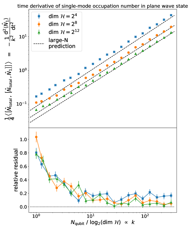
Figure 6: Comparing our analytical predictions for the lifetime of plane waves to results obtained from simulated realisations of low numbers of overlapping qubits. The upper panel displays the expectation value of the bi-commutator of the occupation number operator $\hat{N}_{1}$, representing e.g. a Fourier mode $\bm{k}_{1}$, with the total occupation number operator $\hat{N}_{\mathrm{total}}$ in the Fourier space shell to which $\bm{k}_{1}$ belongs, as a function of the ratio $N_{s}/n_{s}$ (which is proportional to the shell radius $k_{s}$). This bi-commutator is proportional to the second time derivative of the expectation value of $\hat{N}_{1}$, and can hence be used to define a characteristic lifetime for the plane wave state $\ket{\bm{k}_{1}}$, as we have done in Section 4.2. The expectation values are taken wrt. the state $\ket{\bm{k}_{1}}$ and wrt. the CRSV-embedding. Symbols represent results obtained from our simulations (cf. A) and the dashed lines are the asymptotic results obtained in C.2. The lower panel shows relative residuals between the two.

To investigate the impact of holography on the dynamics of our field further, we study the behaviour of plane wave states. Unfortunately, the vacuum state of our Hamiltonian is not an eigenstate of the occupation number operators $\hat{N}_{\bm{p}}$ of any of our overlapping Fourier modes $\bm{p}$. As a consequence, we cannot create a state in which a single mode is excited by acting on the vacuum state with a creation operator $\hat{c}_{\bm{p}}^{\dagger}\,$. Instead, we proceed as follows to define a state which approximates a plane wave excitation of our field with energy $\bm{p}$:

• First we consider the subspace of states $\ket{\phi}$ with $\hat{N}_{\bm{p}}\ket{\phi}=+\ket{\phi}$. These are the states in which we would measure the occupation number of $\bm{p}$ to be 1.

• In this subspace, we find the states that minimize $\left|\frac{\mathrm{d}^{2}}{\mathrm{d}t^{2}}\bra{\phi}\hat{N}_{\bm{p}}\ket{\phi}\right|$. These plane wave candidate states will be most stable in time. (Note that $\frac{\mathrm{d}}{\mathrm{d}t}\bra{\phi}\hat{N}_{\bm{p}}\ket{\phi}\equiv 0$ for all eigenstates of $\hat{N}_{\bm{p}}$.)

• Condition B) is still satisfied by an entire subspace of states (cf. C.2), and our final selection step is to choose the candidate state that has the lowest energy expectation value $\bra{\phi}\hat{H}\ket{\phi}$ .

We denote the state defined through conditions A) - C) with $\ket{\bm{p}}$ and we consider it as the closest equivalent our theory has to the standard plane wave state $\hat{c}_{\bm{p}}^{\dagger}\ket{0}$ for the non-overlapping Weyl field. We then estimate a characteristic time scale for the stability of this plane wave via the equation

$$\frac{1}{T_{\mathrm{scramble}}^{2}}\equiv-\mathbb{E}\left\{\frac{\mathrm{d}^{2}}{\mathrm{d}t^{2}}\bra{\psi_{\mathbf{p}}}\hat{N}_{\mathbf{p}}\ket{\psi_{\mathbf{p}}}\right\}\ .$$ (66)

Here the expectation value $\mathbb{E}\{\cdot\}$ is with respect to the random vectors $\bm{v}_{\bm{p}}$ and $\bm{w}_{\bm{p}}$ that were used to define the Pauli algebra of the mode $\bm{p}$ in the JLC-embedding (cf. Section 3). Note that the different Fourier space shells in our construction do not overlap. Hence, the total occupation number within each individual shell is conserved, and the power that is lost in the mode $\bm{p}$ over time is isotropically scrambled to other modes in the same Fourier space shell $s$. In C.2 we derive analytically that $T_{\mathrm{scramble}}$ for the mode $\bm{p}$ is given in terms of the parameters of our construction by

$$T_{\mathrm{scramble}}\approx 2\pi^{2}\sqrt{\alpha}\left(\frac{\Lambda_{\mathrm{Planck}}}{\Lambda_{\mathrm{UV}}}\right)^{2}\frac{N_{\mathrm{dof},\psi}}{N_{\mathrm{total}}}\sqrt{\frac{L}{k_{s}}}\ ,$$ (67)

where the quantities appearing in this equation where introduced in Section 3, and represent

• $\alpha$: relative width of the Fourier space shell $s$,

• $\Lambda_{\mathrm{UV}}/\Lambda_{\mathrm{Planck}}$: UV-cutoff of our field in Planck units,

• $N_{\mathrm{dof},\psi}$: number of degrees of freedom (qbits) present in our field

• $N_{\mathrm{total}}$: total number of degrees of freedom present in the Universe,

• $L$: IR-cutoff,

• $k_{s}$: central radius of the Fourier space shell $s$.

Our analytical results are approximations that hold in the limit $n_{s}\rightarrow\infty$, $N_{s}\rightarrow\infty$. In Figure 6 we compare those analytical predictions to results obtained from low-dimensional simulations of overlapping qubits (cf. A), and we find that they are already accurate for quite low numbers of qubits - see e.g. the green triangles in Figure 6, which were obtained from simulating only $12$ overlapping qubits.

Equation 67 is the relation we have used to derive our results in Table 1 and Figure 4. In Figure 4 we show $cT_{\mathrm{scramble}}$ for different UV-cuts. In that figure we also indicate the typical energies and travel distances of neutrinos emitted by a number of identified and resolved sources. The existence of solar neutrinos seems to demand that neutrino effective field theory already breaks down at $k_{\mathrm{UV}}<10^{-3}k_{\mathrm{Planck}}$. This is even more drastic when considering cosmic neutrino observations: we summarize the UV-cuts required to allow the existence of different observed fermion signals with know and located sources in Table 1, and the observation of a $\sim 290\,$TeV neutrino emitted from the blazar TXS 0506+056 [49] requires $k_{\mathrm{UV}}<470k_{\mathrm{LHC}}$, i.e. only a few orders of magnitude above modern particle physics experiments. As we discussed in Section 3.4, the breakdown of our effective theory beyond that energy should happen either as a sharp cutoff, or as a transition to super-holographic mode overlaps for modes with $|\bm{k}|>k_{\mathrm{UV}}\,$. This is because any modes present beyond $k_{\mathrm{UV}}$ need to be squeezed into a small part of the field’s Hilbert space in order to still satisfy the cosmic Bekenstein bound.

Note again, that the above considerations assume a ratio of $N_{\mathrm{dof},\psi}/N_{\mathrm{total}}\sim 0.01$ between the degrees of freedom present in a single neutrino field and the total degrees of freedom present in the Universe. In Section 3.3 we argued that this is a realistic estimate, assuming that Bosonic fields can be modelled via generalised Pauli operators (GPU [63, 12, 13]) with similar holographic mode overlaps.

4.3 Consistency with the cosmic ray spectrum

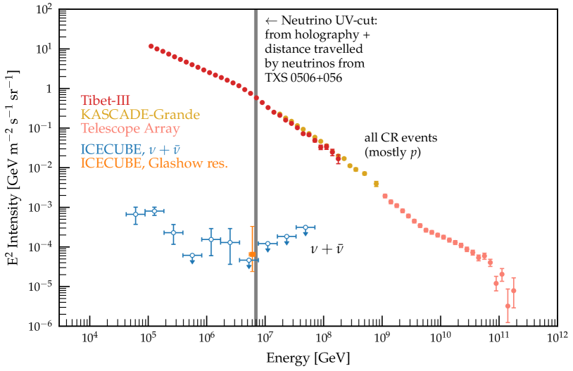
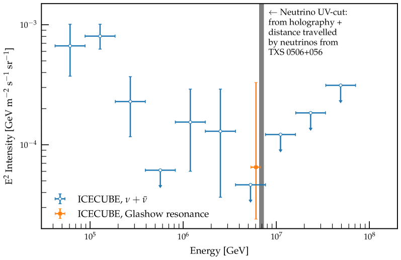
Figure 7: Top panel: Cosmic ray flux (more concretely the $E^{2}$-Intensity, which is defined as $E^{2}\,\mathrm{d}N/\mathrm{d}E\mathrm{d}A\mathrm{d}t\mathrm{d}\Omega$) as a function of particle energy; using data and tools compiled by [67] as well as observations reported by [68]. Lower Panel: Zoom into the neutrino contributions to the cosmic ray spectrum. The grey vertical band indicates the neutrino UV-cut we have derived in Section 4.2. The width of the band is an estimate of the mistake we make by assuming a static Universe. But note that a number of other simplified assumptions may also significantly impact our results.

As we discussed in the previous subsection, when we interpret our construction of the holographic Weyl field as a model for neutrinos then the fact that a $290\,$TeV neutrino has been observed from the far away blazar TXS 0506+056 indicates that neutrino physics should have a UV-cut of $k_{\mathrm{UV}}<470\,k_{\mathrm{LHC}}$ (where we again take $k_{\mathrm{LHC}}=14\,$TeV). Above that threshold we expect a rather sharp cutoff or at least a super-holographic behaviour of the neutrino fields, because whatever modes are present above $k_{\mathrm{UV}}$ need to be squeezed into a very small part of the total Hilbert space in order not to violate the Bekenstein bound.

Of course, our calculation has a number of caveats and relies on a number of modelling choices. We list several of these in Section 8, but the two main shortcomings of our model are that it assumes a static background space time (whereas the cosmos has significantly expanded in the time it took for neutrinos from TXS 0506+056 to arrive on earth), and that we implement a naive, equal-time version of holography instead of quantizing our field on a light-sheet. The UV-cut $k_{\mathrm{UV}}<470k_{\mathrm{LHC}}\,$ may change once these shortcomings are corrected. But our current result does at least seem to be consistent with current intensity limits for the cosmic neutrino flux.

In Figure 7 we have used tools and data compiled by [67] (which includes data from the databases [69, 70, 71]) as well as observations reported by [68] to display current measurements of the intensities observed in different cosmic ray species as a function of particle energy. To date the IceCube experiment [72] has only established upper limits for neutrino flux beyond the UV-cut we derived - cf. the blue, open circles in both panels of Figure 7, which represent direct neutrino detections and the vertical grey band which indicates our result from the previous subsection. So far, the event that comes closest to our limit is an indirect detection of an excitation of the Glashow resonance which presumably took place in Earth’s atmosphere and which has produced a shower of secondary particles which was observed in IceCube (cf. orange square; [68]). This event indicates that electroweak theory is valid until shortly before the energy where our holographic theory for neutrinos needs to break down. Again, this comparison hinges on a number of assumptions, part of which we already know to be rather simplistic. To obtain an estimate of the impact of assuming a static space time, we re-derive our previous UV-cut when taking the travel distance from TXS0506+056 to be the distance between us and the blazar at the time when the observed high energy neutrino was emitted. This indeed moves the UV-cut to higher energies, and the width of the grey band in Figure 7 represents that shift. Of course, we could also directly calculate the travel time of neutrinos from TXS0506+056 and use that to derive a UV-cut. But that would also be a simplification, because we still wouldn’t properly quantize our field on an expanding background. So for now, we stick with the above rough estimate of the impact of cosmic expansion. Another obstacle for further analysis is the stark Lorentz symmetry breaking of our theory close the the UV-cut Section 3.4. A better approximation of Lorentz invariance may be achieved by quantizing the field on light-sheets and by replacing the sharp UV cutoff with a transition to super-holographic mode overlaps. We leave this for future work.

In the upper panel of Figure 7 we also display measurements of cosmic ray flux that are attributed to cosmic protons (using data from the Tibet-III [73], KASCADE-Grande [74] and Telescope Array [75] experiments; as compiled by [67]). The measurements extend to much higher energies than the holographic UV-cut we derived for neutrinos, which seems to indicate that in QCD the breakdown of holography happens at higher energies. There is a number of subtleties which at the moment prevent us from drawing more concrete conclusions from this high energy proton flux. First, protons are composite particles and we did not investigate how to describe such composite states within our framework. Quark confinement, and the fact that quarks have fractional electric charges, will plausibly prevent individual proton constituents from scrambling in the same way that individual neutrino excitations do. The energy of a proton also does not directly translate to similar energies for the proton constituents. Finally, it is a possibility that holography indeed breaks down at different energies for different parts of the standard model. A direct derivation of a QCD UV scale from the travel distances of highly energetic protons (as we did in the previous subsection for neutrinos) is complicated by the fact that high energy protons scatter with the cosmic microwave background [76, 77]. This mimics to some extent the plane wave scrambling we have derived here. Though in our construction that scrambling would not reduce proton energy, but instead create a background of diffuse, highly energetic particles. For these reasons, we do not take the existence of proton cosmic rays above our neutrino cutoff as a significant problem for our model.

Finally, note that some of the high-energy neutrinos detected by IceCube may be associated with distant gamma ray bursts (GRBs). E.g. a neutrino with an energy of $\sim 60\,$TeV may be associated with a GRB that was located to be at redshift $z=1.38$ [58]. If we assume this association to be correct, then we could also use this pairing to derive a UV-cut for our holographic model of neutrinos. Estimating our systematic uncertainty due to assuming a static Universe in the same way as above would lead to an interval $390\,k_{\mathrm{LHC}}\lesssim k_{\mathrm{UV}}\lesssim 601\,k_{\mathrm{LHC}}\,$, which encompasses our fiducial result $k_{\mathrm{UV}}\approx 500\,k_{\mathrm{LHC}}$. The authors of [58] also report an extreme event of a $\sim 1800\,$TeV neutrino that may be associated with a GRB at a redshift of $z=3.93\,$. Our way of estimating the impact of cosmic expansion is likely inaccurate for a source at such a high redshift. If we nevertheless employ that estimate again, and if we assume that the association of said neutrino with the high redshift GRB is indeed correct, we arrive at $128\,k_{\mathrm{LHC}}\lesssim k_{\mathrm{UV}}\lesssim 283\,k_{\mathrm{LHC}}\,$. Such a range would indeed be in tension with the neutrino spectrum displayed in Figure 7, but we deem our calculations unreliable in this situation. To adequately apply our framework to high-redshift sources, we would not just need to reformulate it on an expanding background, but we would also have to implement the covariant entropy bound (i.e. area scaling on light-sheets) instead of the equal-time area scaling present in our current model. As mentioned above, we leave this for future work.

5 Real-space anti-commutator

Let us rewrite ($\hat{c}$-part of) the real-space field as

$$\hat{\psi}^{c}(x) \approx\sum_{\mathrm{shell}\ s}\frac{1}{(k_{s}V)^{\frac{1}{2}}}\sum_{\bm{p}\in s}\hat{c}_{\bm{p}}(t)\ u(\bm{p})\ e^{i\bm{p}\bm{x}}\ ,$$ (68)

where we again made explicit that the field is a sum over independent (non-overlapping) Fourier space shells $s$, and where we assumed that all momenta $\bm{p}$ in one shell $s$ have similar absolute values $|\bm{p}|\approx k_{s}$ .

To asses how much the qubit overlap changes the behaviour of our field wrt. the non-overlapping case, let us consider the equal-time anti-commutator of $\psi^{c}$ and the $\hat{c}$-part of the momentum field, $i\psi_{\alpha}^{c}(\bm{x})^{\dagger}$,

$$\{i\psi_{\alpha}^{c}(\bm{x})^{\dagger},\psi_{\beta}^{c}(\bm{y})\} =i\sum_{\mathrm{shell}\ s}\frac{1}{k_{s}V}\sum_{\bm{p},\bm{q}\in s}\{\hat{c}_{\bm{p}}^{\dagger},\hat{c}_{\bm{q}}\}\ u_{\alpha}(\bm{p})^{\dagger}u_{\beta}(\bm{q})\ e^{-i\bm{p}\bm{x}+i\bm{q}\bm{y}}$$ (69)

$$=i\sum_{\mathrm{shell}\ s}\frac{1}{k_{s}V}\sum_{\bm{p},\bm{q}\in s,\bm{p}\neq\bm{q}}\{\hat{c}_{\bm{p}}^{\dagger},\hat{c}_{\bm{q}}\}\ u_{\alpha}(\bm{p})^{\dagger}u_{\beta}(\bm{q})\ e^{-i\bm{p}\bm{x}+i\bm{q}\bm{y}}\ +$$

$$\ \ +\frac{i}{V}\sum_{\bm{p}}\ \frac{u_{\alpha}(\bm{p})^{\dagger}u_{\beta}(\bm{p})}{|\bm{p}|}\ e^{-i\bm{p}(\bm{x}-\bm{y})}\ .$$

In particular, let us look at the trace of this wrt. the spinor components,

$$\sum_{\alpha}\{i\psi_{\alpha}^{c}(\bm{x})^{\dagger},\psi_{\alpha}^{c}(\bm{y})\} =\frac{i}{2}\sum_{\mathrm{shell}\ s}\frac{1}{k_{s}V}\sum_{\bm{p},\bm{q}\in s,\bm{p}\neq\bm{q}}\braket{z_{\bm{p}}}{z_{\bm{q}}}\ u(\bm{p})^{\dagger}u(\bm{q})\ e^{-i\bm{p}\bm{x}+i\bm{q}\bm{y}}$$ (70)

$$\ \ +i\delta_{D}(\bm{x}-\bm{y})$$

$$\equiv iC(\bm{x},\bm{y})+i\delta_{D}(\bm{x}-\bm{y})\ .$$

The second term in the last line of Equation 70 would be the standard result in the case of independent qubits, while the first term is a correction due to qubit overlap. Because of the stochastic way by which we have embedded the individual qubit operators $\hat{c}_{\bm{p}},\hat{c}_{\bm{p}}^{\dagger}$ into the physical Hilbert space, the correction $C(\bm{x},\bm{y})$ is in fact a (classical) random variable. It can be shown to have vanishing expectation value, and its variance is given by

$$\mathbb{E}\left[|C(\bm{x},\bm{y})|^{2}\right] =\frac{1}{4}\sum_{\mathrm{shell}\ s}\frac{\epsilon_{s}^{2}}{k_{s}^{2}V^{2}}\sum_{\bm{p},\bm{q}\in s,\bm{p}\neq\bm{q}}|u(\bm{p})^{\dagger}u(\bm{q})|^{2}\ ,$$ (71)

where $\epsilon_{s}^{2}=\mathbb{E}(|\langle z_{\bm{p}}|z_{\bm{q}}\rangle|^{2})$ is the variance of the overlap between two qubits in the same shell. As we show in B.5, this variance is given by

$$\epsilon_{s}^{2}=\frac{2}{n_{s}}=\frac{1}{\pi L^{2}k_{s}\Delta_{s}}\ ,$$ (72)

where $n_{s}$ is again the effective number of qubits within the physical Hilbert space of shell $s$ (cf. Section 3). Recall also, that the number of actual (overlapping) qubits within shell $s$ is given by

$$N_{s}=\frac{4\pi k_{s}^{2}\Delta_{s}V}{(2\pi)^{3}}\ .$$ (73)

We can hence re-write the variance of $C(\bm{x},\bm{y})$ as

$$\mathbb{E}\left[|C(\bm{x},\bm{y})|^{2}\right] =\frac{1}{4}\sum_{\mathrm{shell}\ s}\frac{\epsilon_{s}^{2}}{V^{2}}N_{s}^{2}\frac{1}{N_{s}^{2}}\sum_{\bm{p},\bm{q}\in s,\bm{p}\neq\bm{q}}\frac{|u(\bm{p})^{\dagger}u(\bm{q})|^{2}}{k_{s}^{2}}$$ (74)

$$\approx\frac{1}{4}\sum_{\mathrm{shell}\ s}\frac{\epsilon_{s}^{2}}{V^{2}}\left(\frac{4\pi k_{s}^{2}\Delta_{s}V}{(2\pi)^{3}}\right)^{2}\int\frac{\mathrm{d}\Omega_{\bm{p}}\mathrm{d}\Omega_{\bm{q}}}{(4\pi)^{2}}\frac{|u(\bm{p})^{\dagger}u(\bm{q})|^{2}}{k_{s}^{2}}$$

$$\equiv\frac{A}{16\pi^{4}}\sum_{\mathrm{shell}\ s}k_{s}^{4}\epsilon_{s}^{2}\Delta_{s}^{2}\ .$$

Here we have introduced

$$A \equiv\frac{1}{(4\pi)^{2}}\int\mathrm{d}\Omega_{\bm{p}}\mathrm{d}\Omega_{\bm{q}}\frac{|u(\bm{p})^{\dagger}u(\bm{q})|^{2}}{k_{s}^{2}}$$ (75)

$$=\frac{1}{(4\pi)^{2}}\int\mathrm{d}\theta_{1}\sin\theta_{1}\mathrm{d}\phi_{1}\int\mathrm{d}\theta_{2}\sin\theta_{2}\mathrm{d}\phi_{2}\ \left|\cos\frac{\theta_{1}}{2}\cos\frac{\theta_{2}}{2}+e^{i(\phi_{2}-\phi_{1})}\sin\frac{\theta_{1}}{2}\sin\frac{\theta_{2}}{2}\right|^{2}$$

$$=\frac{1}{2}\ .$$

We can hence conclude that

$$\mathbb{E}\left[|C(\bm{x},\bm{y})|^{2}\right] =\frac{1}{32\pi^{5}L^{2}}\sum_{\mathrm{shell}\ s}k_{s}^{3}\Delta_{s}$$ (76)

$$\approx\frac{1}{32\pi^{5}L^{2}}\int_{0}^{\Lambda_{\mathrm{UV}}}\mathrm{d}k\ k^{3}=\frac{\Lambda_{\mathrm{UV}}^{4}}{128\pi^{5}L^{2}}$$

$$\Rightarrow\sqrt{\mathbb{E}\left[|C(\bm{x},\bm{y})|^{2}\right]} =\frac{1}{\sqrt{128\pi^{5}}}\frac{\Lambda_{\mathrm{UV}}^{2}}{L}\ .$$ (77)

Note that - while the propagator $C$ does depend in $\bm{x}$ and $\bm{y}$ - it’s average amplitude between two points is completely independent of those points and their separation. So our construction induces a long-range correlation in the spinor field $\psi$ .

To asses the severity of this effect let us introduce a finite smoothing scale to the real space field, i.e. we consider

$$\hat{\psi}_{R}^{c}(x) =\sum_{\mathrm{shell}\ s}\sum_{\bm{p}\in s}\ \frac{e^{-\frac{1}{2}(|\bm{p}|\cdot R)^{2}}}{(|\bm{p}|V)^{\frac{1}{2}}}\ \hat{c}_{\bm{p}}(t)\ u(\bm{p})\ e^{i\bm{p}\bm{x}}\ ,$$ (78)

and similarly for the $\hat{d}$-part of the field. This will change the trace of the anti-commutator to

$$\sum_{\alpha}\{i\psi_{R,\alpha}^{c}(\bm{x})^{\dagger},\psi_{R,\alpha}^{c}(\bm{y})\}\ =\ iC_{R}(\bm{x},\bm{y})+\frac{i}{\sqrt{(4\pi)^{3}R^{6}}}\ e^{-\frac{1}{4R^{2}}|\bm{x}-\bm{y}|^{2}}$$ (79)

$$\equiv\ iD_{R}(\bm{x},\bm{y})\ ,$$

where the variance of $C_{R}$ is now given by

$$\mathbb{E}\left[|C_{R}(\bm{x},\bm{y})|^{2}\right] \approx\frac{1}{32\pi^{5}L^{2}}\int_{0}^{\Lambda_{\mathrm{UV}}}\mathrm{d}k\ k^{3}\ e^{-k^{2}R^{2}}\approx\frac{1}{16\pi^{5}L^{2}R^{4}}$$ (80)

as long as $R\gg 1/\Lambda_{\mathrm{UV}}$ . We can then compare the long-range anti-commutator $C_{R}(\bm{x},\bm{y})$ to the local anti-commutators $D_{R}(\bm{x},\bm{x})$ and $D_{R}(\bm{y},\bm{y})$ by considering the ratio

$$\frac{\mathbb{E}\left[|C_{R}(\bm{x},\bm{y})|^{2}\right]}{\mathbb{E}\left[D_{R}(\bm{x},\bm{x})\right]\ \mathbb{E}\left[D_{R}(\bm{y},\bm{y})\right]}\ =\ \left(\frac{2R}{\pi L}\right)^{2}\ .$$ (81)

So the qubit overlap only significantly impacts the anti-commutation behaviour of the field on scales $R$ that are comparable to the IR scale $L$ . The above expression still assumes that our field constitutes the only degrees of freedom in the Universe. Assuming that the degrees of freedom of all types of fields (including spacetime degrees of freedom) individually satisfy an area law scaling, the more general result would be

$$\frac{\mathbb{E}\left[|C_{R}(\bm{x},\bm{y})|^{2}\right]}{\mathbb{E}[D_{R}(\bm{x},\bm{x})]\ \mathbb{E}[D_{R}(\bm{y},\bm{y})]}\ =\ \frac{N_{\mathrm{dof,total}}}{N_{\mathrm{dof},\psi}}\left(\frac{2R}{\pi L}\right)^{2}\ ,$$ (82)

where $N_{\mathrm{dof,total}}$ are the total number of degrees of freedom present in the Universe and $N_{\mathrm{dof},\psi}$ are the degrees of freedom contributed by the field $\psi$ . Choosing $L$ again as the co-moving size of our future particle horizon (which is finite in a dark energy dominated Universe), one would expect a $\sim 1\%$ effect on scales $R\sim 25\ \sqrt{N_{\mathrm{dof},\psi}/N_{\mathrm{dof,total}}}$ Mpc. As before, the reason why the presence of other degrees of freedom enhances the effects of holography is that the $N_{s}$ qubits in each shell $s$ then need to be squeezed into an even smaller number of effective qubits $n_{s}$ in order to still satisfy the Bekenstein bound.

6 Alternative modelling choices

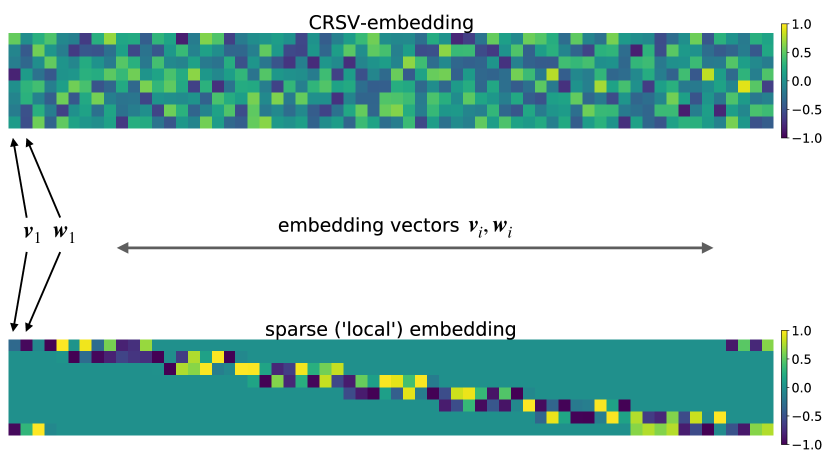
Figure 9: Sketch comparing our fiducial embedding scheme (”CRSV-embedding”) to an alternative scheme investigated in Section 6. See main text of Section 6.1 for details.

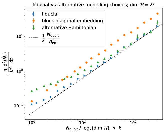
Figure 10: Same as Figure 6, but comparing our fiducial model to alternative analysis choices. See main text of Section 6 for details. Note that due to numerical limitations we needed to reduce the amount of simulations run for our alternative Hamiltonian operator, such that for large ratios $N_{s}/n_{s}$ the results shown here are only averaged over $64$ (instead of $640$) realisations. This is why some of the green triangles display larger error bars than the simulation results obtained for the other modelling choices.

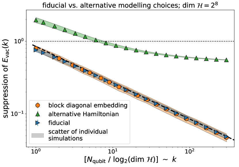
Figure 11: Same as Figure 5, but comparing our fiducial model to alternative analysis choices. See main text of Section 6 for details.

6.1 non-isotropic overlaps

Our fiducial method of embedding $N$ qubits into a Hilbert space of dimension $2^{n},\ n<N$, relies on choosing orthonormal pairs of vectors $\bm{v}_{i},\bm{w}_{i}\ (i=1,\dots,N)$ randomly in $\mathbb{R}^{2n}$ and defining the Pauli algebra of the $i$th qubit from these vector pairs via Equations D). The upper panel of Figure 9 displays the $2n\times 2N$ matrix whose columns consist of such such random vector pairs (in that instance, $n=4$ and $N=32$). In our fiducial construction each pair $\bm{v}_{i},\bm{w}_{i}$ represents one Fourier mode of our quantum field in a thin Fourier space shell, and the scalar products between different vector pairs determine how much the corresponding Fourier modes overlap.

The above way of constructing operators for the different field modes leads to mode overlaps that are independent of how far away two wave vectors $\bm{k}$ and $\bm{p}$ are from each other in Fourier space. We want to investigate the impact of such a non-local overlapping structure on some of our results. To do so, we study an alternative embedding scheme in which the vectors $\bm{v}_{i},\bm{w}_{i}$ form a matrix with a sparse structure, as is depicted in the lower panel of Figure 9. Concretely, this structure is obtained by populating elements above and below the diagonal of the embedding matrix such that both horizontally and vertically only one quarter of the matrix elements are non-zero (and we include non-zero elements in the upper right and lower left corners to obtain cyclic symmetry). Such an embedding could e.g. represent a local overlapping structure in a one-dimensional string of field modes. This would in principle not be appropriate in our case since our overlapping modes live in Fourier space shells which can be thought of as approximately two-dimensional. But with this alternative embedding we can nevertheless qualitatively test for differences between the statistically isotropic overlaps of our fiducial model and a more local scheme of overlaps.

In Figure 10 we show how this new embedding scheme impacts the lifetime of plane waves. Modulo a multiplicative factor, this figure displays $\bra{\bm{k}}\mathrm{d}^{2}\hat{N}_{\bm{k}}/\mathrm{d}t^{2}\ket{\bm{k}}$, i.e. the expectation value of the second time derivative of the occupation number operator $\hat{N}_{\bm{k}}$ in a single field mode (modulo a multiplicative factor) as a function of the energy $|\bm{k}|$ of the plane wave state $\ket{\bm{k}}$ wrt. which the expectation value is taken (also modulo a multiplicative factor, since $N_{s}/n_{s}\sim k_{s}$). In Section 4.2 we had used this second derivative as a definition of $1/T_{\mathrm{scramble}}^{2}$, where we took $T_{\mathrm{scramble}}$ to represent a characteristic time scale within which the plane wave will be completely scrambled within its Fourier space shell. The orange circles in Figure 10 represent values for that second time derivative obtained from averaging $640$ simulated realisations of the new embedding scheme, while the blue triangles use our fiducial scheme and the dashed line represents the analytical prediction derived in C.2. In the limit of large ratios $N_{s}/n_{s}$ the second time derivative of $\hat{N}_{\bm{k}}$ is larger in the alternative embedding scheme compared to the fiducial scheme by more than a factor of $2$, indicating a plane wave lifetime that is shorter by about a factor of $1.5$. This seems to indicate that the statistically isotropic CJL-embedding leads to more stable plane waves than a more local embedding scheme. It is however possible that this picture would reverse if we were to consider wave packets instead of plane waves. Many plane waves will be superposed in such a packet in a way that is local in Fourier space, and it may be that local mode overlaps cause such a superposition to become more stable. At this point neither our analytical nor our simulation tools are powerful enough to test this hypothesis in a meaningful way, and such an analysis needs to be carried out in follow-up work.

Finally, we also investigate the impact of the new embedding scheme on the vacuum energy of our field. Figure 11 compares how that energy is suppressed in the different embedding schemes, and surprisingly we find that that suppression is almost identical in both approaches. For the CJL-embedding we had found in C.1 that the vacuum energy suppression only depends on the ratio $N_{s}/n_{s}$. Since our alternative embedding cuts down the non-zero elements of the embedding matrix by the same factor both horizontally and vertically (cf. our sketch in Figure 9), we speculate that the more local overlap structure retains the same effective ratio of $N_{s}/n_{s}$, and hence retains the same amount of vacuum energy suppression. We however do not repeat our calculations of C.1 for the new embedding scheme, and a more thorough investigation is again postponed to follow-up work.

6.2 alternative Hamiltonian

We also want to consider an alternative, more general form for the Hamiltonian of our field. In this section we thus take the Hamiltonian in one Fourier space shell $s$ to be given by

$$\hat{H}_{s} =\sum_{\bm{q},\bm{k}\in s}A_{\bm{q}\bm{k}}\left\{\left(\hat{c}_{\bm{q}}^{\dagger}\hat{c}_{\bm{k}}-\frac{1}{2}\right)+\left(\hat{d}_{\bm{q}}^{\dagger}\hat{d}_{\bm{k}}-\frac{1}{2}\right)\right\}\ ,$$ (83)

where we choose the ansatz $A_{\bm{q}\bm{k}}=\mathcal{N}_{s}\braket{z_{\bm{k}}}{z_{\bm{q}}}$, such that the coupling of any two Fourier modes in the Hamiltonian is proportional to the overlap of these modes within the CRSV-embedding. The time evolution of $\hat{c}_{\bm{k}}$ with this modified Hamiltonian is given by

$$\frac{\mathrm{d}\hat{c}_{\bm{p}}}{\mathrm{d}t} =i\left[\hat{H}_{s},\hat{c}_{\bm{p}}\right]$$ (84)

$$=\frac{i\mathcal{N}_{s}}{2}\sum_{\bm{q},\bm{k}\in s}\braket{z_{\bm{k}}}{z_{\bm{q}}}\left\{\braket{z_{\bm{k}}^{*}}{z_{\bm{p}}}\hat{c}_{\bm{q}}^{\dagger}-\braket{z_{\bm{q}}}{z_{\bm{p}}}\hat{c}_{\bm{k}}\right\}\ .$$

Now remember that we had represented the annihilation operators $\hat{c}_{\bm{q}}$ by matrices

$$\hat{c}_{\bm{q}}=\frac{1}{2}\sum_{j=1}^{2n}\braket{e_{j}}{z_{\bm{q}}}\bm{C}_{j}\ ,$$ (85)

where $\bm{C}_{j}$ are generators of the Clifford algebra in $2n$ dimensions and $\ket{e_{j}}$ are an orthonormal basis in $\mathbb{R}^{2n}$. As we had already discussed in Section 3, Equation 85 constitutes a stochastic embedding, because the vectors $\ket{z_{\bm{q}}}$ are chosen stochastically in the CRSV-algorithm. But at least on average we would like the right-hand side of Equation 84 to equal $-i|\bm{p}|\hat{c}_{\bm{p}}$, which would be the time derivative of the standard, non-overlapping annihilation operators. This can be achieved by properly choosing the normalisation factor $\mathcal{N}_{s}\,$. First, let us calculate the average operator that would appear on the right-hand side of Equation 84. To do so, we will keep the embedding of the operator $\hat{c}_{\bm{p}}$ fixed, i.e. we fix the coefficients $\braket{e_{j}}{z_{\bm{p}}}$, and we will average over the embedding of the other operators, i.e. over the coefficients $\braket{e_{j}}{z_{\bm{q}}}$, $\braket{e_{j}}{z_{\bm{k}}}$ with $\bm{q}\neq\bm{p}\neq\bm{k}$. It can then be shown that

$$\mathbb{E}\left[\frac{\mathrm{d}\hat{c}_{\bm{p}}}{\mathrm{d}t}\right]_{\braket{e_{j}}{z_{\bm{p}}}\ \mathrm{fixed}} =-\frac{i\mathcal{N}_{s}}{2}\ \hat{c}_{\bm{p}}\ \sum_{\bm{q}\in s}\mathbb{E}\left[|\langle z_{\bm{q}}|z_{\bm{p}}\rangle|^{2}\right]_{\braket{e_{j}}{z_{\bm{p}}}\ \mathrm{fixed}}$$ (86)

$$=-2i\mathcal{N}_{s}\hat{c}_{\bm{p}}\ \left\{\frac{(N_{s}-1)}{n_{s}}+1\right\}$$

$$\approx-2i\mathcal{N}_{s}\ \hat{c}_{\bm{p}}\ \left\{1+\frac{k_{s}L}{2\pi^{3}}\right\}\ .$$

So in order for the average time evolution to equal that of the standard Weyl field, we need to choose

$$\mathcal{N}_{s}=\frac{k_{s}}{2\left(\frac{(N_{s}-1)}{n_{s}}+1\right)}\ .$$ (87)

Such a normalisation factor was not necessary in our fiducial Hamiltonian, because there $\mathbb{E}[\mathrm{d}\hat{c}_{\bm{p}}/\mathrm{d}t]=-i|\bm{p}|\hat{c}_{\bm{p}}$ was already satisfied to begin with (we do not explicitly show this here, but it is straight forward to demonstrate).

The green triangles in Figure 10 show $\bra{\bm{k}}\mathrm{d}^{2}N_{\bm{k}}/\mathrm{d}t^{2}\ket{k}$ as a function of $N_{s}/n_{s}$ in simulated realisations of overlapping qubits for the alternative Hamiltonian discussed above. For large ratios $N_{s}/n_{s}$ this second time derivative seems to approach the same asymptotic behaviour as plane waves with our fiducial Hamiltonian (blue triangles, and the dashed line which represents our analytical result from C.2). One may speculate that this is a result of our choice for the normalisation constant $\mathcal{N}_{s}$ which ensures that the average dynamics of the field modes is the same for our fiducial and alternative Hamiltonian. We however do not extend our analytical calculations from C.2 to the more general Hamiltonian and cannot confirm this speculation at this point. The fact that the lifetime of plane waves doesn’t seems to be significantly altered between our fiducial Hamiltonian and a more general one nevertheless lends a degree of robustness to one of our key results. Of course, we have only considered a rather restricted generalisation and a much more general class of Hamiltonians should be investigated in follow-up work. Note in particular that (as we discuss in Section 7) the ansatz of our paper needs to be more thoroughly motivated by concepts of quantum mereology, in which a given Hamiltonian dictates which degrees of freedom are good candidates for semi-classical field degrees of freedom and thus how the Hamiltonian itself looks like in terms of these degrees of freedom.

Finally, while plane waves behave quite similarly with our alternative Hamiltonian, the energy eigenspectrum seems to be significantly altered. The green triangles in Figure 11 show the suppression of vacuum energy with our alternative Hamiltonian, and it is much less severe than that present with our fiducial Hamiltonian. Note also, that the scatter of vacuum energy (wrt. different realisations of the CRSV-embedding) is much reduced for the alternative Hamiltonian. Again, we do not attempt to extend our calculations of C.1 to the more general Hamiltonian and postpone a more thorough analysis to follow-up work. In particular, at this point it is not clear which form of the Hamiltonian would be motivated by a more thorough integration of our work into a quantum mereology framework.

7 Why these random overlaps? Context within quantum mereology

In this section, we would like to embed our construction into the context of quantum mereology [65]. We will argue, that our investigation is in a sense mereology done the wrong way around. This will also shed light on a peculiar feature of our model of a holographic Weyl field: the fact that it contains a stochastic element in the form of randomly chosen embeddings of the field modes into the smaller, physical Hilbert space.

Let us again consider a thin shell $s$ in Fourier space with radius $k_{s}$ and width $\Delta_{s}\ll k_{s}$. The particle-part of our field (and similarly, the anti-particle-part) consists of

$$N_{s}\,\approx\,\frac{4\pi k_{s}^{2}\Delta_{s}}{(2\pi/L)^{3}}\,\propto\,k_{s}^{2}\Delta_{s}$$ (88)

Fourier modes $\bm{p}\in s$, where $L$ is the IR-cut of our theory. In the usual Weyl field, each of these modes corresponds to one independent qubit in the overall Hilbert space. This would however lead to a volume scaling of the field’s number of degrees of freedom. To achieve an (approximate) area scaling, we instead sought to represent the field’s Fourier space shell $s$ in a Hilbert space of dimension $2^{n_{s}}<2^{N_{s}}$ with

$$n_{s}\propto k_{s}\Delta_{s}\ .$$ (89)

We did so by choosing $2n_{s}$ Clifford generators $\bm{C}_{j}$ in the Hilbert space of dimension $2^{n_{s}}$ and then representing the Pauli algebra of each field mode $\bm{p}$ (for the particle-, or $c$-part of the field) as

$$\bm{\sigma}_{x,\bm{p}}^{c}\equiv\sum_{j=1}^{2n}\braket{e_{j}}{v_{\bm{p}}}\bm{C}_{j}\ \ ,\ \ \bm{\sigma}_{y,\bm{p}}^{c}\equiv\sum_{j=1}^{2n}\braket{e_{j}}{w_{\bm{p}}}\bm{C}_{j}\ \ ,\ \ \bm{\sigma}_{z,\bm{p}}^{c} =-i\bm{\sigma}_{x,\bm{p}}^{c}\bm{\sigma}_{y,\bm{p}}^{c}\ ,$$

where $\braket{e_{j}}{v_{\bm{p}}}$ and $\braket{e_{j}}{w_{\bm{p}}}$ are the $j$th components of two orthonormal vectors $\bm{v}_{\bm{p}}$ and $\bm{w}_{\bm{p}}$ that are randomly chosen in $\mathbb{R}^{2n_{s}}$. The Johnson-Lindenstrauss theorem (cf. our B.3) together with the results of [24] (cf. our Section 3.1) then guarantees that the field modes for two different $\bm{p}\neq\bm{q}$ in the same shell $s$ almost anti-commute (up to a small $\epsilon$, cf. our Equation 53). We have referred to the deviations from perfect anti-commutation as the overlap between the modes $\bm{p}$ and $\bm{q}$. That overlap is a stochastic quantity itself, since it is proportional to the scalar products between the random vectors $\bm{v}_{\bm{p}},\bm{w}_{\bm{p}}$ and $\bm{v}_{\bm{q}},\bm{w}_{\bm{q}}$ .

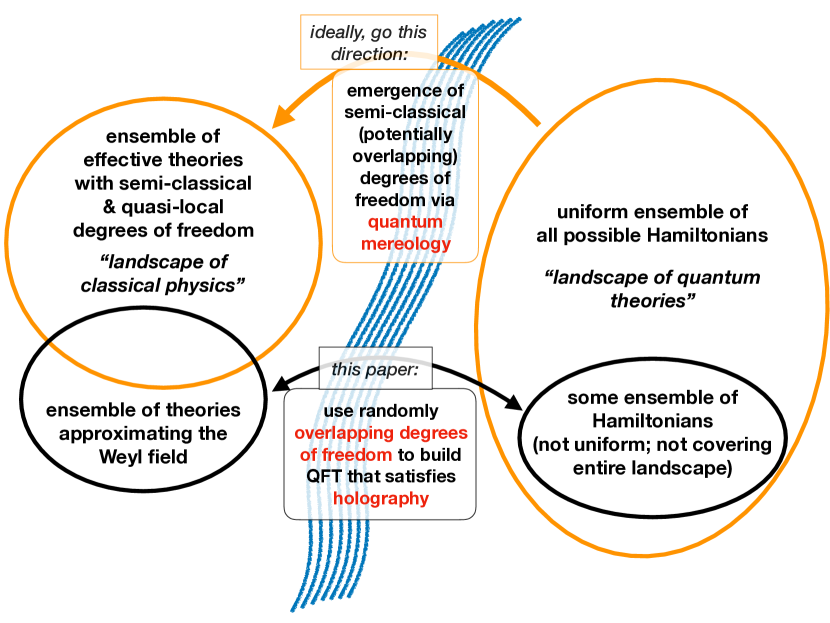
Figure 12: Putting our work into the context of the quantum mereology / quantum first program [63, 65, 43, 64, 21]. The latter conjectures, that classical physics and in particular classical, local degrees of freedom emerge from an abstract quantum theory (specified through a Hamiltonian operator in some Hilbert space) by decomposing the Hilbert space of that theory into factors that satisfy certain classicality conditions (upper, orange part of the sketch). Finding and implementing such a mereology algorithm is challenging [65], and our work (lower, black part of the sketch) does not quite tackle this task (cf. our discussion in Section 7). But our insights and the tools we developed can assist future implementations of the quantum mereology program. And as an additional product, we managed to derive a concrete phenomenology of the holographic principle.

Why these random overlaps? Why should the true, low-energy EFT of quantum gravity be described by a model with stochastic ingredients, and what is the mechanism to choose the random vectors $\bm{v}_{\bm{p}},\bm{w}_{\bm{p}}$ ? We conjecture that the answer to these questions can be found in the concept of quantum mereology. In [65] the authors consider general quantum theories, which are defined by an arbitrary Hilbert space $\mathcal{H}$ as well as a Hamilton operator $\hat{H}$ on that Hilbert space. The ensemble $\{\mathcal{H},\hat{H}\}$ can be considered as the landscape of all possible quantum theories. An arbitrarily picked point in that landscape is not equipped with any pre-defined notion of degrees of freedom, i.e. the Hilbert space $\mathcal{H}$ does not have any a priori decomposition $\mathcal{H}=\mathcal{H}_{1}\otimes\mathcal{H}_{2}\otimes\dots$ into factors that represent individual degrees of freedom. The authors of [65] also assume that there are no pre-defined observables other then the Hamiltonian $\hat{H}$. Instead, they argue that such operators as well as a preferred Hilbert space factorisation should emerge, by demanding that - under the evolution dictated by $\hat{H}$ - the emergent factors and operators should behave in a quasi-classical way. More concretely, they propose and implement the following algorithm for quantum mereology:

• Choose a candidate factorisation $\mathcal{H}=\mathcal{H}_{1}\otimes\mathcal{H}_{2}\otimes\dots$ .

• Among all observables of the form $\hat{O}=\hat{O}_{1}\otimes\hat{O}_{2}\otimes\dots$ , find the one that is most compatible with the Hamiltonian $\hat{H}$ (i.e. whose commutator with $\hat{H}$ has the smallest operator norm).

• Consider a set of product states $\{\ket{\psi}=\ket{\psi}_{1}\otimes\ket{\psi}_{2}\otimes\dots\}$ that correspond to peaked configurations in the observables $\hat{O}_{i}$ , i.e. the $\ket{\psi}_{i}$ are superpositions of the eigenstates of $\hat{O}_{i}$ that are concentrated around one of the eigenvalues of $\hat{O}_{i}$.

• Evaluate two measures of classicality for this candidate factorisation: A) how slowly does entanglement entropy grow when starting in the states $\{\ket{\psi}\}$, and B) how slowly do the peaked states $\{\ket{\psi}\}$ disperse (when viewed as wave packets in the eigenspectrum of the operators $\hat{O}_{i}$). These criteria have been interpreted by [65] as follows: A) measures the robustness of the observables $\hat{O}_{i}$ towards decoherence, and B) measures predictability in the sense of asking how long it takes for peaked states in the observables $\hat{O}_{i}$ to disperse.

• Find the factorisation $\mathcal{H}=\mathcal{H}_{1}\otimes\mathcal{H}_{2}\otimes\dots$ that maximises some joint measure of criteria A) and B). This is the emergent, semi-classical factorisation of $\mathcal{H}$. And the operators $\hat{O}_{i}$ measure observable degrees of freedom living on the factors $\mathcal{H}_{i}$ .

Originally, [65] implemented their mereology algorithm for the situation where $\mathcal{H}$ is only split into two factors (a system and an environment), but we want to consider their ideas here in the context of many degrees of freedom. In particular, we would like to interpret the $\hat{O}_{i}$ as local degrees of freedom in some effective field theory. To do that, we would need to complement the original algorithm by some locality criterion. But such a generalised version of mereology may be difficult to realise, because it is not guaranteed that an arbitrary Hamiltonian admits a factorisation in which dynamics are local. The authors of [78] have shown that such a factorisation rarely exists, and that it is essentially unique if it exists. Though the situation may be not as dire as these results indicate, because according to the findings of [79] factorisations in which a given Hamiltonian appears approximately local do exist for quite general ensembles of Hamiltonians.

One way to increase the success probability of finding degrees of freedom with quasi-local dynamics when given an arbitrary Hamiltonian is to make the mereology algorithm more flexible: instead of insisting that the Hilbert space $\mathcal{H}$ be split into an exact factorisation and that the observables $\hat{O}_{i}$ have exactly vanishing (anti-)commutators, we may instead task mereology with finding operators $\hat{O}_{i}$ that are only quasi-commuting - similar to the mode operators $\hat{c}_{\bm{p}},\hat{d}_{\bm{p}}$ of our holographic Weyl field. (Technically, $\hat{c}_{\bm{p}},\hat{d}_{\bm{p}}$ are of course not local because they are the Fourier space degrees of freedom. But also the real space degrees of our field suffer random overlaps, as is demonstrated by our investigation of the real space anti-commutator in Section 5.) In the following, we will assume that the mereology algorithm is given this additional leeway and that, given a Hamiltonian $\hat{H}$, it identifies EFT degrees of freedom $\hat{O}_{i}$ that have local dynamics but that can have small non-zero overlaps.

Now note that we have started the mereology algorithm by randomly picking a point $(\mathcal{H},\hat{H})$ in the landscape of quantum theories. Even the points on that landscape with the same Hilbert space $\mathcal{H}$ will still vary in their Hamiltonian $\hat{H}$, i.e. these points will result in different EFT degrees of freedom $\hat{O}_{i}$ . So the mereology algorithm we conjectured above will map an ensemble $\{\hat{H}\}$ of Hamiltonian operators to an ensemble $\{\{\hat{O}_{1}\,,\,\hat{O}_{2}\,,\,\dots\,\}_{\hat{H}}\}$ of sets of quasi-classical degrees of freedom, with each set $\{\hat{O}_{1}\,,\,\hat{O}_{2}\,,\,\dots\,\}_{\hat{H}}$ corresponding to a different quasi-local EFT. In C, we find evidence that our model of the Weyl field with overlapping degrees of freedom indeed fits into such a perspective. We show there that the Hamiltonian $\hat{H}_{s}$ in one Fourier space shell $s$ of our field can be written as

$$\hat{H}_{s} \propto\sum_{j,k=1}^{n}\left(M_{jk}\hat{A}_{j}\hat{A}_{k}+X_{jk}\hat{A}_{j}\hat{A}_{k}^{\dagger}-X_{jk}^{*}\hat{A}_{j}^{\dagger}\hat{A}_{k}-M_{jk}^{*}\hat{A}_{j}^{\dagger}\hat{A}_{k}^{\dagger}\right)\ ,$$ (90)

where the $\hat{A}_{j},\hat{A}_{j}^{\dagger}$ are non-overlapping creation and annihilation operators and $M_{jk},X_{ij}$ are random coefficients that depend on the vectors $\bm{v}_{\bm{p}},\bm{w}_{\bm{p}}$ from above. In particular, these coefficients have zero mean and identical variances (see C for more details). So the Hamiltonian above is that of a non-local Heisenberg model with 2-site interactions and randomly drawn interaction coefficients. This is a very general ensemble of theories! And nevertheless, with the help of overlapping degrees of freedom, this can be reformulated into an ensemble of theories that approximates the standard Weyl field. If we interpret this as an instance of quantum mereology, then the randomness of the embedding vectors $\bm{v}_{\bm{p}},\bm{w}_{\bm{p}}$ simply appears to be a result of sampling from a more general landscape of quantum theories.

There are a number of caveats to this admittedly enthusiastic interpretation of our results, which we list in the following.

• We have only shown in a quite limited way, that our model indeed approximates the Weyl field. We demonstrated that plane waves in our field can have cosmic life times (cf. Section 4), that anti-commutators between Fourier modes are tiny (cf. Section 3.2), and that notable differences to the real-space propagator only appear at cosmological scales (cf. Section 5). We have not studied the full dynamics of our field, and have only limited reason to claim that the locality of that dynamics is preserved.

• We present a link between a somewhat general ensemble of quantum theories and an ensemble of theories approximating a quasi-local EFT, but we do not demonstrate that this link is made via any sort of mereology algorithm.

• While we did reduce our construction to a quite general ensemble of Heisenberg models, this is still far from sampling the space of all possible Hamiltonians. In particular, our results are restricted to Heisenberg models with only 2-site interactions, and we still assume different Fourier space shells to be uncoupled. (Though note that [79] showed that Hamiltonians with 2-site interactions are approximately unitary equivalent to the ensemble of all possible Hamiltonians in $\mathbb{C}^{2^{n}}$ with exponentially small error in the limit $n\rightarrow\infty\,$.)

Part of these caveats are summarised by our sketch in Figure 12. Ideally, the program of quantum mereology would be implemented by sampling from the landscape of all possible, abstract Hamiltonians (right hand-side of the sketch) and then applying a mereology algorithm to re-interpret the latter as an ensemble of theories with quasi-classical degrees of freedom and dynamics (left hand-side of the sketch). If we view the process of mereology as bridging a river between the landscape of abstract quantum theories and the landscape of potential quasi-classical physics, then the approach of this paper has rather been the following: we float down the river and throw ropes to either side of it, in the hopes that they stick somewhere (lower part of the sketch; and creating a concrete implementation of holography in the process). As a result we sample neither on the right nor on the left hand-side of the sketch quite the ensembles of theories we would like to sample. Nevertheless, we consider our findings as strong evidence, that the mereology program can work in principle. And the framework of overlapping degrees of freedom we have developed may assist in future implementations of that program.

8 Discussion

Since Section 1 included a detailed overview of our results, we will summarise them here only very briefly, and instead focus on open questions. The essential results are:

• We have introduced a modified version of the Weyl field whose effective degrees of freedom obey an approximate area scaling (exact area scaling in Fourier space), and that satisfies the Bekenstein bound for the total degrees of freedom inside the cosmic horizon.

• We find that each pair of Fourier modes of that field still behaves like a pair of almost independent, non-overlapping degrees of freedom ($|\{\hat{c}_{\bm{p}},\hat{c}_{\bm{q}}\}|\sim 10^{-43}$ at LHC energies). The real space anti-commutator obtains a stochastic, non-local correction which however becomes significant only on cosmological scales.

• We define plane wave states in our holographic field and find that they have a finite lifetime. In particular, the power in a wave of energy $\bm{p}$ is scrambling to modes of similar absolute value $|\bm{p}|$. We find that this is not in contradiction to observed cosmological sources of highly energetic neutrino emission as long as our effective theory breaks down at energies $k_{\mathrm{UV}}<470k_{\mathrm{LHC}}\,$. We argued that this is still consistent with current bounds on the validity regime of electroweak theory from observations of the high-energy cosmic neutrinos. But a potential tension arises if we naively apply our calculations to a highly energetic neutrino that according to [58] may be associated with a gamma ray burst detected at a high redshift ($z\approx 3.93$).

• We have motivated our construction via quantum mereology, i.e. using the idea that EFT degrees of freedom should emerge from an abstract theory of quantum gravity by finding quasi-classical Hilbert space decompositions.

• We also find that vacuum energy is significantly reduced in our construction, e.g. by a factor $\sim 10^{-30}$ if $k_{\mathrm{UV}}\sim k_{\mathrm{Planck}}$ and by $\sim 10^{-25}$ if $k_{\mathrm{UV}}\sim 470k_{\mathrm{LHC}}$ (which corresponds to an overall suppression of $\sim 10^{-74}$ compared to a naive calculation with $k_{\mathrm{UV}}=k_{\mathrm{Planck}}$ and no holography). Neither of this is enough to be relevant for the cosmological constant problem.

All of these findings depend on a number of parameters and modelling choices, and a large number of questions remain unaddressed. We list those in the following:

• Several of our results assumed a ratio of $N_{\mathrm{dof},\psi}/N_{\mathrm{dof,total}}\sim 0.01$, i.e. that our holographic field makes up $\sim 1\%$ of all degrees of freedom in the Universe. In Section 3.3 we have only given a heuristic justification for that number. Our argument did take into account the fact that Bosonic fields may need to be modelled via generalised Pauli operators (as e.g. done by [63, 12, 13]) and that such fields would contribute significantly more degrees of freedom to the Universe’s total budget than Fermionic fields. But a more thorough analysis, that e.g. more closely examines potential overlaps between different matter fields, is needed.

• While we have considered one alternative to our fiducial Hamiltonian and found that both Hamiltonians lead to similar plane wave lifetimes, we have not demonstrated that there isn’t any other alternative Hamiltonian for the holographic Weyl field that more closely preserves the classical, non-overlapping dynamics.

• As explained in Section 7, the spirit of our analysis is a reverse (and thus unsuccessful) version of the quantum mereology program, which aims to describe the emergence of classical degrees of freedom from abstract quantum theories (cf. Figure 12). At the same time, the technology we have developed for describing overlapping degrees of freedom may help future analyses to follow mereology in the right direction.

• We have studied the dynamics of plane waves, but particle propagation would more realistically be described via wave packets. The latter would be described by superpositions of plane waves, but the overlap between the different Fourier modes of our field may cause such overlaps to display non-trivial behaviour.

• To define the lifetime of plane waves we have only considered averages of the second time derivative of mode occupation numbers $\hat{N}_{\bm{p}}\,$. Significant scatter around those averages could lead to further effective changes to the dispersion relation of plane waves.

• We have investigated the suppression of vacuum energy of our field. But our results do in principle allow us to calculate the entire energy eigenspectrum of the field. A more detailed study of that spectrum may reveal even more observational signatures of holography.

• We have considered only one alternative to our fiducial way of making degrees of freedom overlap in such a way that an approximate area scaling is reached. There maybe a multitude of alternatives, and some of those may preserve classical, non-overlapping dynamics more closely, especially when investigating those dynamics beyond plane waves.

• We have implemented a naive, equal-time version of holography instead of imposing a holographic scaling of degrees of freedom on a light-sheet. We have also quantized our field in a static, non-expanding background. Both of these simplification impair the applicability of our calculations to high-redshift sources such as the ones reported by [58].

• We have imposed a sharp UV cutoff in our model. Instead, UV regularisation could also take place as a transition from holographic to super-holographic mode overlaps, such that all modes above the regularisation scale $k_{\mathrm{UV}}$ are squeezed into a small part of the overall Hilbert space. Such a regularisation may decrease the severity Lorentz symmetry breaking, especially when paired with a quantisation that implements the covariant entropy bound on light-sheets instead of our naive equal-time area scaling.

• According to [8, 41, 42] the degrees of freedom underlying effective field theory should deplete even more quickly with energy than the naive area scaling $n_{s}\sim k_{s}\Delta_{s}$ we have assumed. Note also that [42] investigate a number of observational consequences of EFT mode depletion which we have not considered. At the same time, a modified version of our construction may serve as a model that implements the ideas put forward by [41, 42].

The above points constitute a multitude of open questions and potential problems for our construction. Nevertheless, the tools we have developed here may serve to open a fruitful new pathway towards studying observational signatures of the holographic principle.

Data availability

Python tools to reproduce our results (analytical predictions and simulated realisations of overlapping qubits) are publicly available at https://github.com/OliverFHD/GPUniverse . We also provide data measured in a suite of simulations of overlapping qubits in that repository.

References

Appendix A Simulated realisations of the CRSV-embedding

We have complemented the analytical calculations presented in C and in the main text with simulated realisations the the CRSV-embedding of $N$ qubits into a Hilbert space of dimension $2^{n},\ n<N$. Comparing our analytical calculations to these simulations in particular allows us to determine how quickly the asymptotic limit in which these calculations are valid is reached.

To generate overlapping qubits, we follow very closely to the CRSV-procedure described in Section 3. This requires us to

• choose $2n$ generators of Clifford algebra in the Hilbert space $\mathbb{C}^{2^{n}}$; we do this via the iterative algorithm proposed by [84],

• generate $2N$ random vectors on the unit sphere in $\mathbb{R}^{2n}$,

• in the planes spanned by each pair of these vectors generate an orthonormal basis by applying the Gram-Schmidt algorithm to the original pairs.

If $\bm{C}_{j}$ are the Clifford generators and $\bm{v},\bm{w}$ is one of the orthonormal vector pairs, a Pauli algebra that represents one qubit can be obtained via

$$\bm{\sigma}_{x}^{c}\equiv\sum_{j=1}^{2n}v^{j}\bm{C}_{j}\ \ ,\ \ \bm{\sigma}_{y,\bm{p}}^{c}\equiv\sum_{j=1}^{2n}w^{j}\bm{C}_{j}\ \ ,\ \ \bm{\sigma}_{z,\bm{p}}^{c} =-i\bm{\sigma}_{x,\bm{p}}^{c}\bm{\sigma}_{y,\bm{p}}^{c}\ .$$ (91)

Each pair of orthonormal vector then generates one qubit, and as has been demonstrated by [24] (see also the calculations we present in Section 3.1, B.1, B.3) the anti-commutator between the lowering and raising operators of different qubits will depend on the scalar products between the random vectors that were used to construct the Pauli operators corresponding to those qubits.

Due to computational constraints, we were only able to simulate quite low numbers of qubits. In the most extensive case we simulated $N=3600$ qubits squeezed into a Hilbert space of $\log_{2}$-dimension $n=12$ (i.e. $\dim\mathcal{H}=2^{12}=4096$). It however turns out that this is already enough to reach the asymptotic regime in which our calculations based on random matrix theory are valid - see e.g. Figure 5 and Figure 6 as well as their descriptions in the main text. Each simulation was run $640$ times and these figures present averages of our quantities of interest over these repeated runs.

To implement the above calculations we made use of the python packages cupy (package enabling computations with graphical processing units; see https://cupy.dev) as well as numpy [80] and scipy [81]. Our simulation code is publicly available within our GPUniverse package (https://github.com/OliverFHD/GPUniverse).

Appendix B Random vectors on the unit sphere and the Johnson-Lindenstrauss theorem

B.1 Moments on the unit sphere

Let us consider two random vectors $\bm{v}_{1},\bm{v}_{2}\in\mathbb{R}^{n}$ that are normalised, $|\bm{v}_{1}|^{2}=1=|\bm{v}_{2}|^{2}$ , and that are otherwise drawn from a uniform distribution on the unit sphere. Because of symmetry reasons (e.g. mirroring $\bm{v}_{1}$ wrt. the hyperplane orthogonal to $\bm{v}_{2}$) the expectation value $\mathbb{E}[\bm{v}_{1}\cdot\bm{v}_{2}]$ must vanish. In other words: on average the two vectors will be orthogonal.

To calculate the variance of $\bm{v}_{1}\cdot\bm{v}_{2}$ we then only have to compute the 2nd moment of $\cos\theta$, where $\theta$ is the angle of points on the $n$-dimensional unit sphere wrt. an arbitrary axis. This 2nd moment is given by

$$\frac{\int_{0}^{\pi}\mathrm{d}\theta\ (\sin\theta)^{n-2}\ (\cos\theta)^{2}}{\int_{0}^{\pi}\mathrm{d}\theta\ (\sin\theta)^{n-2}}=\frac{\frac{1}{2}\sqrt{\pi}\ \Gamma\left(\frac{n-1}{2}\right)/\Gamma\left(\frac{n}{2}+1\right)}{\sqrt{\pi}\ \Gamma\left(\frac{n-1}{2}\right)/\Gamma\left(\frac{n}{2}\right)}$$ (92)

So the variance of the scalar product between two random unit vectors in $\mathbb{R}^{n}$ is given by

$$\mathrm{Var}(\bm{v}_{i}\cdot\bm{v}_{j})=\frac{\Gamma\left(\frac{n}{2}\right)}{2\Gamma\left(\frac{n}{2}+1\right)} =\frac{1}{n}\ .$$ (93)

Now consider a single random vector $\bm{v}$ drawn uniformly on the unit sphere in $\mathbb{R}^{n}$. For some of the results of this paper we need to calculate moments like $\mathbb{E}[v_{1}^{2}v_{2}^{2}]$, where $v_{i}$ it the $i$th component of $\bm{v}$. This amounts to computing

$$\frac{\int_{0}^{\pi}\mathrm{d}\theta\ \sin^{n-2}\theta\ \cos^{2}\theta\sin^{2}\theta\int_{0}^{\pi}\mathrm{d}\phi\ \sin^{n-3}\phi\ \cos^{2}\phi}{\int_{0}^{\pi}\mathrm{d}\theta\ \sin^{n-2}\theta\int_{0}^{\pi}\mathrm{d}\phi\ \sin^{n-3}\phi}$$

$$=\frac{\frac{1}{2}\sqrt{\pi}\ \Gamma\left(\frac{n+1}{2}\right)/\Gamma\left(\frac{n+2}{2}+1\right)}{\sqrt{\pi}\ \Gamma\left(\frac{n-1}{2}\right)/\Gamma\left(\frac{n}{2}\right)}\frac{\frac{1}{2}\sqrt{\pi}\ \Gamma\left(\frac{n-2}{2}\right)/\Gamma\left(\frac{n-1}{2}+1\right)}{\sqrt{\pi}\ \Gamma\left(\frac{n-2}{2}\right)/\Gamma\left(\frac{n-1}{2}\right)}$$

$$=\frac{1}{4}\frac{\Gamma\left(\frac{n}{2}\right)}{\Gamma\left(\frac{n}{2}+2\right)}=\frac{1}{n\left(n+2\right)}\ .$$ (94)

Similarly (but simpler) the moment $\mathbb{E}[v_{1}^{4}]$ requires calculation of

$$\frac{\int_{0}^{\pi}\mathrm{d}\theta\ \sin^{n-2}\theta\ \cos^{4}\theta}{\int_{0}^{\pi}\mathrm{d}\theta\ \sin^{n-2}\theta} =\frac{\int_{0}^{\pi}\mathrm{d}\theta\ \left[\sin^{n-2}\theta\ -\sin^{n}\theta\right]\ \cos^{2}\theta}{\int_{0}^{\pi}\mathrm{d}\theta\ \sin^{n-2}\theta}$$ (95)

$$=\frac{1}{n}-\frac{1}{2}\frac{\Gamma\left(\frac{n-1}{2}+1\right)/\Gamma\left(\frac{n}{2}+2\right)}{\Gamma\left(\frac{n-1}{2}\right)/\Gamma\left(\frac{n}{2}\right)}$$

$$=\frac{1}{n}-\frac{n-1}{n\left(n+2\right)}=\frac{3}{n(n+2)}\ .$$

And the 6th moment $\mathbb{E}[v_{1}^{6}]$ is given by

$$\frac{\int_{0}^{\pi}\mathrm{d}\theta\ \sin^{n-2}\theta\ \cos^{6}\theta}{\int_{0}^{\pi}\mathrm{d}\theta\ \sin^{n-2}\theta} =\frac{\int_{0}^{\pi}\mathrm{d}\theta\ \left[\sin^{n-2}\theta\ -2\sin^{n}\theta+\sin^{n+2}\theta\right]\ \cos^{2}\theta}{\int_{0}^{\pi}\mathrm{d}\theta\ \sin^{n-2}\theta}$$ (96)

$$=\frac{1}{n}+\frac{1}{2}\frac{\Gamma\left(\frac{n}{2}\right)}{\Gamma\left(\frac{n-1}{2}\right)}\left[\frac{\Gamma\left(\frac{n-1}{2}+2\right)}{\Gamma\left(\frac{n}{2}+3\right)}-2\frac{\Gamma\left(\frac{n-1}{2}+1\right)}{\Gamma\left(\frac{n}{2}+2\right)}\right]$$

$$=\frac{15}{n\left(n+2\right)\left(n+4\right)}\ .$$

We also need to calculate moments of the form $\mathbb{E}[v_{1}^{4}v_{2}^{2}]$. This amounts to computing

$$\frac{\int_{0}^{\pi}\mathrm{d}\theta\ \left[\sin^{n}\theta\ -\sin^{n+2}\theta\right]\cos^{2}\theta\int_{0}^{\pi}\mathrm{d}\phi\ \sin^{n-3}\phi\ \cos^{2}\phi}{\int_{0}^{\pi}\mathrm{d}\theta\ \sin^{n-2}\theta\int_{0}^{\pi}\mathrm{d}\phi\ \sin^{n-3}\phi}$$

$$=\frac{1}{4}\left[\frac{\Gamma\left(\frac{n+1}{2}\right)}{\Gamma\left(\frac{n}{2}+2\right)}-\frac{\Gamma\left(\frac{n+3}{2}\right)}{\Gamma\left(\frac{n}{2}+3\right)}\right]\frac{\Gamma\left(\frac{n}{2}\right)}{\Gamma\left(\frac{n+1}{2}\right)}$$

$$=\frac{3}{n\left(n+2\right)\left(n+4\right)}\ .$$ (97)

Finally, we need to calculate moments of the form $\mathbb{E}[v_{1}^{2}v_{2}^{2}v_{3}^{2}]$. This amounts to computing

$$\frac{\int_{0}^{\pi}\mathrm{d}\theta\ \sin^{n+2}\theta\ \cos^{2}\theta\int_{0}^{\pi}\mathrm{d}\phi\ \sin^{n-1}\phi\ \cos^{2}\phi\int_{0}^{\pi}\mathrm{d}\chi\ \sin^{n-4}\chi\ \cos^{2}\chi}{\int_{0}^{\pi}\mathrm{d}\theta\ \sin^{n-2}\theta\int_{0}^{\pi}\mathrm{d}\phi\ \sin^{n-3}\phi\int_{0}^{\pi}\mathrm{d}\chi\ \sin^{n-4}\chi\ \cos^{2}\chi}$$

$$=\frac{1}{8}\frac{\Gamma\left(\frac{n+3}{2}\right)/\Gamma\left(\frac{n+4}{2}+1\right)}{\Gamma\left(\frac{n-1}{2}\right)/\Gamma\left(\frac{n}{2}\right)}\frac{\Gamma\left(\frac{n}{2}\right)/\Gamma\left(\frac{n+1}{2}+1\right)}{\Gamma\left(\frac{n-2}{2}\right)/\Gamma\left(\frac{n-1}{2}\right)}\frac{\Gamma\left(\frac{n-3}{2}\right)/\Gamma\left(\frac{n-2}{2}+1\right)}{\Gamma\left(\frac{n-3}{2}\right)/\Gamma\left(\frac{n-2}{2}\right)}$$

$$=\frac{1}{8}\frac{\Gamma\left(\frac{n}{2}\right)}{\Gamma\left(\frac{n}{2}+3\right)}=\frac{1}{n\left(n+2\right)\left(n+4\right)}$$

B.2 Moments of orthogonal vectors

Consider two random unit vectors $\bm{v},\bm{\tilde{w}}\in\mathbb{R}^{n}$. We can define a $\bm{w}\perp\bm{v}$ via

$$\bm{w} =\bm{\tilde{w}}-(\bm{\tilde{w}}\cdot\bm{v})\,\bm{v}$$

$$\Rightarrow w_{i} =\tilde{w}_{i}-v_{i}\sum_{j}v_{j}\tilde{w}_{j}\ .$$ (99)

Note that $\bm{w}$ is not yet normalised. We will address this missing normalisation later, but for now let us consider joint moments of $\bm{w}$ and $\bm{v}$. We start with

$$\mathbb{E}[w_{1}^{2}v_{1}^{2}] =\mathbb{E}[\tilde{w}_{1}^{2}]\,\mathbb{E}[v_{1}^{2}]-2\mathbb{E}[\tilde{w}_{1}v_{1}^{3}\sum_{j}v_{j}\tilde{w}_{j}]+\mathbb{E}[v_{1}^{4}\sum_{jk}v_{j}v_{k}\tilde{w}_{j}\tilde{w}_{k}]$$ (100)

$$=\mathbb{E}[\tilde{w}_{1}^{2}]\,\mathbb{E}[v_{1}^{2}]-2\mathbb{E}[\tilde{w}_{1}^{2}]\,\mathbb{E}[v_{1}^{4}]+\sum_{j}\mathbb{E}[\tilde{w}_{j}^{2}]\,\mathbb{E}[v_{1}^{4}v_{j}^{2}]$$

$$=\frac{1}{n^{2}}-\frac{6}{n^{2}(n+2)}+\frac{3n-3}{n^{2}\left(n+2\right)\left(n+4\right)}+\frac{15}{n^{2}(n+2)(n+4)}$$

$$=\frac{1}{n^{2}}-\frac{3}{n^{2}\left(n+2\right)}$$

$$=\frac{n-1}{n^{2}(n+2)}\ .$$

We will also require the moment

$$\mathbb{E}[w_{1}^{2}v_{2}^{2}] =\mathbb{E}[\tilde{w}_{1}^{2}]\,\mathbb{E}[v_{2}^{2}]-2\mathbb{E}[\tilde{w}_{1}v_{1}v_{2}^{2}\sum_{j}v_{j}\tilde{w}_{j}]+\mathbb{E}[v_{1}^{2}v_{2}^{2}\sum_{jk}v_{j}v_{k}\tilde{w}_{j}\tilde{w}_{k}]$$ (101)

$$=\mathbb{E}[\tilde{w}_{1}^{2}]\,\mathbb{E}[v_{2}^{2}]-2\mathbb{E}[\tilde{w}_{1}^{2}]\,\mathbb{E}[v_{1}^{2}v_{2}^{2}]+\sum_{j}\mathbb{E}[\tilde{w}_{j}^{2}]\,\mathbb{E}[v_{1}^{2}v_{2}^{2}v_{j}^{2}]$$

$$=\frac{1}{n^{2}}-\frac{2}{n^{2}(n+2)}+\frac{n-2}{n^{2}(n+2)(n+4)}+\frac{6}{n^{2}(n+2)(n+4)}$$

$$=\frac{1}{n^{2}}-\frac{1}{n^{2}(n+2)}$$

$$=\frac{n+1}{n^{2}(n+2)}\ .$$

Finally, we will also need

$$\mathbb{E}[w_{1}w_{2}v_{1}v_{2}] =-\mathbb{E}[\tilde{w}_{1}v_{2}^{2}v_{1}\sum_{j}v_{j}\tilde{w}_{j}]-\mathbb{E}[\tilde{w}_{2}v_{2}v_{1}^{2}\sum_{j}v_{j}\tilde{w}_{j}]+\mathbb{E}[v_{1}^{2}v_{2}^{2}\sum_{jk}v_{j}v_{k}\tilde{w}_{j}\tilde{w}_{k}]$$ (102)

$$=-\mathbb{E}[\tilde{w}_{1}^{2}]\,\mathbb{E}[v_{1}^{2}v_{2}^{2}]-\mathbb{E}[\tilde{w}_{2}^{2}]\,\mathbb{E}[v_{1}^{2}v_{2}^{2}]+\sum_{j}\mathbb{E}[\tilde{w}_{j}^{2}]\,\mathbb{E}[v_{1}^{2}v_{2}^{2}v_{j}^{2}]$$

$$=-\frac{2}{n^{2}(n+2)}+\frac{n-2}{n^{2}(n+2)(n+4)}+\frac{6}{n^{2}(n+2)(n+4)}$$

$$=-\frac{1}{n^{2}(n+2)}\ .$$

For later calculations we actually require the moments between $\bm{v}$ and a normalised version of $\bm{w}$,

$$\bm{\hat{w}} \equiv\frac{\bm{w}}{|\bm{w}|}=\frac{\bm{w}}{\sqrt{1-(\bm{v}\cdot\bm{\tilde{w}})^{2}}}\ .$$ (103)

In the following we approximate such moments as

$$\mathbb{E}[\hat{w}_{i}\hat{w}_{j}v_{k}v_{l}] =\mathbb{E}\left[\frac{w_{i}w_{j}v_{k}v_{l}}{1-(\bm{v}\cdot\bm{\tilde{w}})^{2}}\right]\approx\frac{\mathbb{E}[w_{i}w_{j}v_{k}v_{l}]}{1-\mathbb{E}[(\bm{v}\cdot\bm{\tilde{w}})^{2}]}\ .$$ (104)

Corrections to this approximation will involve moments of at least 68 vector components. Correspondingly these corrections will be of higher order, and vanish in the $n\rightarrow\infty$ limit. Since $\mathbb{E}[(\bm{v}\cdot\bm{\tilde{w}})^{2}]=1/n$, our moments of interest hence become

$$\mathbb{E}[\hat{w}_{1}^{2}v_{1}^{2}] \approx\frac{n-1}{n^{2}(n+2)}\frac{1}{1-1/n}=\frac{1}{n(n+2)}$$ (105)

$$\mathbb{E}[\hat{w}_{1}^{2}v_{2}^{2}] \approx\frac{n+1}{n^{2}(n+2)}\frac{1}{1-1/n}=\frac{n+1}{(n-1)n(n+2)}$$ (106)

$$\mathbb{E}[\hat{w}_{1}\hat{w}_{2}v_{1}v_{2}] \approx-\frac{1}{n^{2}(n+2)}\frac{1}{1-1/n}=\frac{-1}{(n-1)n(n+2)}\ .$$ (107)

Note especially that

$$\mathbb{E}[\hat{w}_{1}^{2}v_{1}^{2}] =\mathbb{E}[\hat{w}_{1}^{2}]\,\mathbb{E}[v_{1}^{2}]+\mathcal{O}\left[\frac{1}{n^{3}}\right]$$ (108)

$$\mathbb{E}[\hat{w}_{1}^{2}v_{2}^{2}] =\mathbb{E}[\hat{w}_{1}^{2}]\,\mathbb{E}[v_{2}^{2}]+\mathcal{O}\left[\frac{1}{n^{3}}\right]$$ (109)

$$\mathbb{E}[\hat{w}_{1}\hat{w}_{2}v_{1}v_{2}] =0+\mathcal{O}\left[\frac{1}{n^{3}}\right]\ .$$ (110)

Together with the fact that $\mathbb{E}[v_{i}\hat{w}_{j}]=0$ we take this as justification to treat $\bm{v}$ and $\bm{\hat{w}}$ as independent random vectors in the large-$n$ limit, and in particular to ignore the mixed moments $\mathbb{E}[\hat{w}_{1}\hat{w}_{2}v_{1}v_{2}]$ in the following calculations.

B.3 The Johnson-Lindenstrauss theorem

We prove here a slightly different version of the JL-theorem than the one considered by [53]:

Theorem Johnson-Lindenstrauss – Consider a $k\times n$ dimensional matrix $\bm{V}=(\bm{v}_{1}\,,\,\dots\,,\,\bm{v}_{n})$, obtained by drawing each element from a standard normal distribution $\mathcal{N}(0,1)$ and then normalising the column vectors of $\bm{V}$ such that $|\bm{v}_{i}|^{2}=1$ . Now take any $n$ vectors $\bm{x}_{1}\,,\,\dots\,,\,\bm{x}_{n}\in\mathbb{R}^{n}$ . As long as

$$k\geq\frac{8}{\epsilon^{2}}\ln\left(\frac{n}{\sqrt{\delta}}\right)$$ (111)

all pairwise squared distances between the $\bm{x}_{i}$ are preserved within precision $\pm\epsilon$ with probability $\geq 1-\delta$ . More precisely,

$$(1-\epsilon)|\bm{x}_{i}-\bm{x}_{j}|^{2}\leq|\bm{Vx}_{i}-\bm{Vx}_{j}|^{2}\leq(1+\epsilon)|\bm{x}_{i}-\bm{x}_{j}|^{2}$$ (112)

for all pairs $\bm{x}_{i},\bm{x}_{j}$ with probability $\geq 1-\delta$ .

An important detail here is the statement that Equation 112 is holds for all pairs. If it would only hold for an individual pair then there would be no reason why $k$ should depend on $n$, since the statement would just be one about random angles in $\mathbb{R}^{k}$ .

To prove this modified version of the JL theorem, we first quote [53] who showed that with the above choice of $\bm{V}$ the probability that Equation 112 is not satisfied for some individual pair of vectors is given by

$$P\left(\left|\frac{|\bm{x}_{i}-\bm{x}_{j}|^{2}-|\bm{Vx}_{i}-\bm{Vx}_{j}|^{2}}{|\bm{x}_{i}-\bm{x}_{j}|^{2}}\right|>\epsilon\right)\leq 2\exp\left(-\frac{k\epsilon^{2}}{4}\right)\ .$$ (113)

With our lower bound on $k$ this becomes

$$P\left(\left|\frac{|\bm{x}_{i}-\bm{x}_{j}|^{2}-|\bm{Vx}_{i}-\bm{Vx}_{j}|^{2}}{|\bm{x}_{i}-\bm{x}_{j}|^{2}}\right|>\epsilon\right) \leq 2\exp\left(-2\ln\left(\frac{n}{\sqrt{\delta}}\right)\right)$$ (114)

$$=\frac{2\delta}{n^{2}}\ .$$

Taking a union bound over all pairs of points the probability of having at least one pair violating Equation 112 is then given by

$$P\left(\left|\frac{|\bm{x}_{i}-\bm{x}_{j}|^{2}-|\bm{Vx}_{i}-\bm{Vx}_{j}|^{2}}{|\bm{x}_{i}-\bm{x}_{j}|^{2}}\right|>\epsilon\ \mathrm{for\ at\ least\ on\ pair}\right) \leq\left(\matrix{n\cr 2}\right)\frac{2\delta}{n^{2}}$$ (115)

$$\leq\delta\ .$$

So Equation 112 is satisfied for all pairs with probability $\geq 1-\delta$ . $\square$

Of course the theorem stated above is only a statement about distances between pairs of vectors, while in Figure 3 or Equation 11 we made statements about the scalar products between pairs of vectors. We simply quote here [52], who have shown that these are two equivalent viewpoints on the JL-theorem. In particular, they showed that

Corollary – Consider the same situation as stated in our above version of the JL-theorem. Then

$$\bm{x}_{i}\cdot\bm{x}_{j}-\epsilon\leq\bm{Vx}_{i}\cdot\bm{Vx}_{j}\leq\bm{x}_{i}\cdot\bm{x}_{j}+\epsilon$$ (116)

for all pairs $\bm{x}_{i},\bm{x}_{j}$ with probability $\geq 1-\delta$ .

If the vectors $\bm{x}_{i}$ are chosen to be orthonormal, this in particular means that $|\bm{Vx}_{i}\cdot\bm{Vx}_{j}|<\epsilon$ , and this is in fact the statement we have used in the main text. There, the anti-commutator between two different, overlapping operators $\hat{c}_{\bm{p}},\hat{c}_{\bm{q}}$ in the same Fourier space shell was given by

$$\{\hat{c}_{\bm{p}}^{\dagger},\hat{c}_{\bm{q}}\} =\frac{\braket{v_{\bm{p}}}{v_{\bm{q}}}+\braket{w_{\bm{p}}}{w_{\bm{q}}}+i\braket{v_{\bm{p}}}{w_{\bm{q}}}-i\braket{w_{\bm{p}}}{v_{\bm{q}}}}{2}\ ,$$ (117)

where $\{\ket{v_{\bm{p}}},\ket{w_{\bm{p}}}\}_{\bm{p}\in s}$ is a set of $2N_{s}$ normalised vectors in $\mathbb{R}^{2n_{s}}$ , $n_{s}$ being the number of physical qubits present in the Fourier space shell $s$ and $N_{s}$ the number of Fourier modes in that shell.

Hence, if in our above formulation of the JL-theorem we set $k=2n_{s}$ and $n=2N_{s}$, and if we draw the $\{\ket{v_{\bm{p}}},\ket{w_{\bm{p}}}\}$ from orthonormal $\{\bm{x}_{i}\}$ via the random matrix $\bm{V}$ described above, then we can derive that

$$|\{\hat{c}_{\bm{p}}^{\dagger},\hat{c}_{\bm{q}}\}| =\frac{|\braket{v_{\bm{p}}}{v_{\bm{q}}}+\braket{w_{\bm{p}}}{w_{\bm{q}}}+i\braket{v_{\bm{p}}}{w_{\bm{q}}}-i\braket{w_{\bm{p}}}{v_{\bm{q}}}|}{2}$$ (118)

$$\leq\frac{|\braket{v_{\bm{p}}}{v_{\bm{q}}}|+|\braket{w_{\bm{p}}}{w_{\bm{q}}}|+|\braket{v_{\bm{p}}}{w_{\bm{q}}}|+|\braket{w_{\bm{p}}}{v_{\bm{q}}}|}{2}$$

$$\leq\epsilon$$

for all mode pairs $\bm{p},\bm{q}$ with probability $>1-\delta$ as long as we choose

$$n_{s}\geq\frac{4}{(\epsilon/2)^{2}}\ln\left(\frac{2N_{s}}{\sqrt{\delta}}\right)=\frac{16}{\epsilon^{2}}\ln\left(\frac{2N_{s}}{\sqrt{\delta}}\right)\ .$$ (119)

For fix $n_{s}$, $N_{s}$ and $\delta$ we can turn this around and compute the smallest mode overlap achievable to be

$$\epsilon_{\mathrm{best}}=\sqrt{\frac{16}{n_{s}}\ln\left(\frac{2N_{s}}{\sqrt{\delta}}\right)}\ .$$ (120)

B.4 Angles between complex vectors

Consider two complex vectors

$$\bm{v}=\bm{x}+i\bm{y}\ \ ,\ \ \bm{w}=\bm{a}+i\bm{b}\ ,$$ (121)

with $\bm{x},\bm{y},\bm{a},\bm{b}\in\mathbb{R}^{n}$ being Gaussian random vectors like we have considered before in this section. Normalising $\bm{v}$ and $\bm{w}$ yields the vectors

$$\bm{\hat{v}}=\frac{\bm{x}+i\bm{y}}{\sqrt{|\bm{x}|^{2}+|\bm{y}|^{2}}}\ \ ,\ \ \bm{\hat{w}}=\frac{\bm{a}+i\bm{b}}{\sqrt{|\bm{a}|^{2}+|\bm{b}|^{2}}}\ .$$ (122)

The Hermitian product between these vectors is

$$\bm{\hat{v}}^{\dagger}\bm{\hat{w}} =\frac{[(\bm{x}^{T}\bm{a})+(\bm{y}^{T}\bm{b})]+i[(\bm{x}^{T}\bm{b})-(\bm{y}^{T}\bm{a})]}{\sqrt{|\bm{x}|^{2}+|\bm{y}|^{2}}\sqrt{|\bm{a}|^{2}+|\bm{b}|^{2}}}\ .$$ (123)

For our derivation of the lifetime of plane waves in the holographic Weyl field in C, we need to calculate the expectation value of $|\bm{\hat{v}}^{\dagger}\bm{\hat{w}}|^{2}$, which is given by

$$\mathbb{E}\left[|\bm{\hat{v}}^{\dagger}\bm{\hat{w}}|^{2}\right] =\frac{\mathbb{E}\left[\{(\bm{x}^{T}\bm{a})+(\bm{y}^{T}\bm{b})\}^{2}\right]}{(|\bm{x}|^{2}+|\bm{y}|^{2})(|\bm{a}|^{2}+|\bm{b}|^{2})}+\frac{\mathbb{E}\left[\{(\bm{x}^{T}\bm{b})-(\bm{y}^{T}\bm{a})\}^{2}\right]}{(|\bm{x}|^{2}+|\bm{y}|^{2})(|\bm{a}|^{2}+|\bm{b}|^{2})}$$

Let us define the vectors

$$\bm{r}\equiv\pmatrix{\bm{x}\cr\bm{y}}\ \ ,\ \ \bm{s}\equiv\pmatrix{-\bm{y}\cr\bm{x}}\ \ ,\ \ \bm{c}\equiv\pmatrix{\bm{a}\cr\bm{b}}\ .$$ (125)

Then Equation B.4 becomes

$$\mathbb{E}\left[|\bm{\hat{v}}^{\dagger}\bm{\hat{w}}|^{2}\right] =\frac{\mathbb{E}\left[(\bm{r}^{T}\bm{c})^{2}\right]}{|\bm{r}|^{2}|\bm{c}|^{2}}+\frac{\mathbb{E}\left[(\bm{s}^{T}\bm{c})^{2}\right]}{|\bm{s}|^{2}|\bm{c}|^{2}}\ .$$ (126)

The terms on the right hand side of this equation are expectation values of products of uniform random vectors on the unit sphere in $\mathbb{R}^{2n}$. Our results from B.1 then tell us that

$$\mathbb{E}\left[|\bm{\hat{v}}^{\dagger}\bm{\hat{w}}|^{2}\right] =\frac{2}{2n}=\frac{1}{n}\ .$$ (127)

B.5 Moments of the overlaps $\braket{z_{\bm{q}}}{z_{\bm{p}}}$

Let $\bm{p}$ be a wave mode located in some Fourier space shell $s$, and remember that $\ket{z_{\bm{p}}}=\ket{v_{\bm{p}}}+i\ket{w_{\bm{p}}}$ with

$$\braket{v_{\bm{p}}}{v_{\bm{p}}}=1=\braket{w_{\bm{p}}}{w_{\bm{p}}}\ \ ,\ \ \braket{v_{\bm{p}}}{w_{\bm{p}}}=0\ .$$ (128)

For another mode $\bm{q}$ in the same shell we have

$$\braket{z_{\bm{q}}}{z_{\bm{p}}} =\left(\,\bra{v_{\bm{q}}}-i\bra{w_{\bm{q}}}\,\right)\left(\,\ket{v_{\bm{p}}}+i\ket{w_{\bm{p}}}\,\right)$$ (129)

$$=\braket{v_{\bm{q}}}{v_{\bm{p}}}+\braket{w_{\bm{q}}}{w_{\bm{p}}}+i\left(\,\braket{v_{\bm{q}}}{w_{\bm{p}}}-\braket{w_{\bm{q}}}{v_{\bm{p}}}\,\right)\ ,$$

while

$$\braket{z_{\bm{q}}^{*}}{z_{\bm{p}}} =\left(\,\bra{v_{\bm{q}}}+i\bra{w_{\bm{q}}}\,\right)\left(\,\ket{v_{\bm{p}}}+i\ket{w_{\bm{p}}}\,\right)$$ (130)

$$=\braket{v_{\bm{q}}}{v_{\bm{p}}}-\braket{w_{\bm{q}}}{w_{\bm{p}}}+i\left(\,\braket{v_{\bm{q}}}{w_{\bm{p}}}+\braket{w_{\bm{q}}}{v_{\bm{p}}}\,\right)\ .$$

For $\bm{q}\neq\bm{p}$ all of the above products between the $\{\ket{v_{\bm{p}}},\ket{w_{\bm{p}}},\ket{v_{\bm{q}}},\ket{w_{\bm{q}}}\}$ have a variance of $1/n_{s}$, where $n_{s}$ is the total number of modes in the shell $s$. At the same time, the covariance between these vector products is $0$.

For the moments of the complex products $\braket{z_{\bm{q}}}{z_{\bm{p}}},\ \braket{z_{\bm{q}}^{*}}{z_{\bm{p}}}$ this means

$$\mathbb{E}\left[\braket{z_{\bm{q}}}{z_{\bm{p}}}^{2}\right] =\frac{1}{2n_{s}}+\frac{1}{2n_{s}}-\frac{1}{2n_{s}}-\frac{1}{2n_{s}}$$ (131)

$$=0$$

$$\mathbb{E}\left[\braket{z_{\bm{q}}^{*}}{z_{\bm{p}}}^{2}\right] =0$$ (132)

$$\mathbb{E}\left[\braket{z_{\bm{q}}}{z_{\bm{p}}}\braket{z_{\bm{q}}^{*}}{z_{\bm{p}}}\right] =\frac{1}{2n_{s}}-\frac{1}{2n_{s}}-\frac{1}{2n_{s}}+\frac{1}{2n_{s}}$$ (133)

$$=0$$

$$\mathbb{E}\left[|\braket{z_{\bm{q}}}{z_{\bm{p}}}|^{2}\right] =\frac{2}{n_{s}}\ =\mathbb{E}\left[|\braket{z_{\bm{q}}^{*}}{z_{\bm{p}}}|^{2}\right]\ .$$ (134)

Appendix C Our construction as a Heisenberg model

In this appendix we will show that the Hamiltonian $\hat{H}_{s}$ in a single Fourier space shell $s$ of our holographic Weyl field can be re-interpreted as that of a Heisenberg model with general non-local, two-site interactions. In a second step we then re-formulate that Heisenberg Hamiltonian to resemble the Hamiltonian of a set of non-interacting spins in a stochastic, spatially varying magnetic field. This will allow us to characterise the energy spectrum of our field, and in particular the average vacuum energy of our construction. Similar calculations will then also yield the typical lifetime of plane wave states.

In Section 3 we had defined

$$\bm{\sigma}_{x,\bm{p}}^{c}\equiv\sum_{j=1}^{2n}\braket{e_{j}}{v_{\bm{p}}}\bm{C}_{j}\ \ ,\ \ \bm{\sigma}_{y,\bm{p}}^{c}\equiv\sum_{j=1}^{2n}\braket{e_{j}}{w_{\bm{p}}}\bm{C}_{j}\ \ ,\ \ \bm{\sigma}_{z,\bm{p}}^{c} =-i\bm{\sigma}_{x,\bm{p}}^{c}\bm{\sigma}_{y,\bm{p}}^{c}$$

as well as

$$\bm{c}_{\bm{p}}=\frac{1}{2}\left(\bm{\sigma}_{x,\bm{p}}^{c}+i\bm{\sigma}_{y,\bm{p}}^{c}\right)\ .$$

(Note the difference with the original CRSV-embedding because we want to produce approximately anti-commuting sets of operators instead of approximately commuting ones.) Each $\bm{p}$ represents one of the overlapping qubits of the $c$-part (i.e. the particle-part) our field. But since the dimension of the Hilbert space of Fourier space shell $s$ is a power of two ($\dim\mathcal{H}_{s}=2^{n_{s}}$) we can also decompose our construction into a set of non-overlapping qubits. Let us e.g. define the creation and annihilation operators of these qubits as

$$\hat{A}_{j}\equiv\frac{1}{2}\left(\bm{C}_{2j-1}+i\bm{C}_{2j}\right)\ ,\ \hat{A}_{j}^{\dagger}\equiv\frac{1}{2}\left(\bm{C}_{2j-1}-i\bm{C}_{2j}\right)$$

$$\Rightarrow\bm{C}_{2j-1}=\hat{A}_{j}+\hat{A}_{j}^{\dagger}\ ,\ \bm{C}_{2j}=-i(\hat{A}_{j}-\hat{A}_{j}^{\dagger})\ .$$

If we furthermore set

$$f_{\bm{p},j}\equiv\braket{e_{2j-1}}{v_{\bm{p}}}+i\braket{e_{2j}}{v_{\bm{p}}}\ ,\ g_{\bm{p},j}\equiv\braket{e_{2j-1}}{w_{\bm{p}}}+i\braket{e_{2j}}{w_{\bm{p}}}$$

then we have

$$\ \ \ \ i\bm{\sigma}_{z,\bm{p}}^{c}$$

$$=\bm{\sigma}_{x,\bm{p}}^{c}\bm{\sigma}_{y,\bm{p}}^{c}$$

$$=\sum_{j=1}^{n}\sum_{k=1}^{n}\left(\braket{e_{2j-1}}{v_{\bm{p}}}\bm{C}_{2j-1}+\braket{e_{2j}}{v_{\bm{p}}}\bm{C}_{2j}\right)\left(\braket{e_{2k-1}}{w_{\bm{p}}}\bm{C}_{2k-1}+\braket{e_{2k}}{w_{\bm{p}}}\bm{C}_{2k}\right)$$

$$=\sum_{j=1}^{n}\sum_{k=1}^{n}\left(f_{\bm{p},j}^{*}\hat{A}_{j}+f_{\bm{p},j}\hat{A}_{j}^{\dagger}\right)\left(g_{\bm{p},k}^{*}\hat{A}_{k}+g_{\bm{p},k}\hat{A}_{k}^{\dagger}\right)$$

$$=\sum_{j=1}^{n}\sum_{k=1}^{n}\left(f_{\bm{p},j}^{*}g_{\bm{p},k}^{*}\hat{A}_{j}\hat{A}_{k}+f_{\bm{p},j}^{*}g_{\bm{p},k}\hat{A}_{j}\hat{A}_{k}^{\dagger}+f_{\bm{p},j}g_{\bm{p},k}^{*}\hat{A}_{j}^{\dagger}\hat{A}_{k}+f_{\bm{p},j}g_{\bm{p},k}\hat{A}_{j}^{\dagger}\hat{A}_{k}^{\dagger}\right)$$

If we define the matrices $\bm{M}$ and $\bm{X}$ via

$$M_{jk}\equiv-i\sum_{\bm{p}\in s}f_{\bm{p},j}^{*}g_{\bm{p},k}^{*}\ ,\ X_{jk}\equiv-i\sum_{\bm{p}\in s}f_{\bm{p},j}^{*}g_{\bm{p},k}$$ (136)

then the Hamiltonian in the Fourier space shell $s$ (with $\Delta_{s}\ll k_{s}$) becomes

$$\hat{H}_{s} \approx\frac{k_{s}}{2}\sum_{\bm{p}\in s}\bm{\sigma}_{z,\bm{p}}^{c}$$ (137)

$$=\frac{k_{s}}{2}\sum_{j,k=1}^{n}\left(M_{jk}\hat{A}_{j}\hat{A}_{k}+X_{jk}\hat{A}_{j}\hat{A}_{k}^{\dagger}-X_{jk}^{*}\hat{A}_{j}^{\dagger}\hat{A}_{k}-M_{jk}^{*}\hat{A}_{j}^{\dagger}\hat{A}_{k}^{\dagger}\right)\ .$$

So the Hamiltonian in each Fourier space shell of our construction is equivalent to that of a general, non-local Heisenberg model with 2-site interactions.

C.1 Energy spectrum of the holographic field

Using the anti-commutation relations between the (non-overlapping) operators $\hat{A}_{j},\hat{A}_{k},\hat{A}_{j}^{\dagger},\hat{A}_{k}^{\dagger}$ we can reformulate Equation 137 as

$$\hat{H}_{s} =\frac{k_{s}}{2}\sum_{j,k=1}^{n}\left\{\frac{M_{jk}-M_{kj}}{2}\hat{A}_{j}\hat{A}_{k}-\frac{M_{jk}^{*}-M_{kj}^{*}}{2}\hat{A}_{j}^{\dagger}\hat{A}_{k}^{\dagger}\right\}$$ (138)

$$\ \ \ +\frac{k_{s}}{2}\sum_{j,k=1}^{n}\left\{\frac{1}{2}X_{jk}\hat{A}_{j}\hat{A}_{k}^{\dagger}+\frac{1}{2}X_{jk}\delta_{jk}-\frac{1}{2}X_{jk}\hat{A}_{k}^{\dagger}\hat{A}_{j}\right\}$$

$$\ \ \ -\frac{k_{s}}{2}\sum_{j,k=1}^{n}\left\{\frac{1}{2}X_{jk}^{*}\hat{A}_{j}^{\dagger}\hat{A}_{k}+\frac{1}{2}X_{jk}^{*}\delta_{jk}-\frac{1}{2}X_{jk}^{*}\hat{A}_{k}\hat{A}_{j}^{\dagger}\right\}\ ,$$

Note that

$$\sum_{j=1}^{n}X_{jj} =-i\sum_{\bm{p}\in s}\sum_{j=1}^{n}\left\{\braket{e_{2j}}{v_{\bm{p}}}-i\braket{e_{2j+1}}{v_{\bm{p}}}\right\}\left\{\braket{e_{2j}}{w_{\bm{p}}}+i\braket{e_{2j+1}}{w_{\bm{p}}}\right\}$$ (139)

$$=-i\sum_{\bm{p}\in s}\left[\braket{v_{\bm{p}}}{w_{\bm{p}}}+i\sum_{j=1}^{n}\left\{\braket{e_{2j}}{v_{\bm{p}}}\braket{e_{2j+1}}{w_{\bm{p}}}-\braket{e_{2j+1}}{v_{\bm{p}}}\braket{e_{2j}}{w_{\bm{p}}}\right\}\right]$$

$$=\sum_{\bm{p}\in s}\sum_{j=1}^{n}\left[\braket{e_{2j}}{v_{\bm{p}}}\braket{e_{2j+1}}{w_{\bm{p}}}-\braket{e_{2j+1}}{v_{\bm{p}}}\braket{e_{2j}}{w_{\bm{p}}}\right\}$$

which is real, such that the terms proportional to $X_{jk}\delta_{jk}$ and $X_{jk}^{*}\delta_{jk}$ in the second line of Equation 138 cancel each other. We can then write the shell-Hamiltonian as

$$\hat{H}_{s}=\frac{k_{s}}{2}\sum_{j,k=1}^{n}\left\{\frac{M_{jk}-M_{kj}}{2}\hat{A}_{j}\hat{A}_{k}+\frac{M_{kj}^{*}-M_{jk}^{*}}{2}\hat{A}_{j}^{\dagger}\hat{A}_{k}^{\dagger}\right\}$$

$$\ \ \ +\frac{k_{s}}{2}\sum_{j,k=1}^{n}\left\{\frac{X_{jk}+X_{kj}^{*}}{2}\hat{A}_{j}\hat{A}_{k}^{\dagger}-\frac{X_{kj}+X_{jk}^{*}}{2}\hat{A}_{j}^{\dagger}\hat{A}_{k}\right\}$$

$$\equiv\frac{k_{s}}{2}\left(\hat{A}_{1}^{\dagger},\ \dots\ ,\ \hat{A}_{n}^{\dagger},\ \hat{A}_{1},\ \dots\ ,\ \hat{A}_{n}\right)\pmatrix{-\frac{\displaystyle\bm{X}^{T}+\bm{X}^{*}}{\displaystyle 2}&\frac{\displaystyle\bm{M}^{\dagger}-\bm{M}^{*}}{\displaystyle 2}\cr&\cr\frac{\displaystyle\bm{M}-\bm{M}^{T}}{\displaystyle 2}&\frac{\displaystyle\bm{X}+\bm{X}^{\dagger}}{\displaystyle 2}}\pmatrix{\hat{A}_{1}\cr\dots\cr\hat{A}_{n}\cr\hat{A}_{1}^{\dagger}\cr\dots\cr\hat{A}_{n}^{\dagger}}$$

$$=\frac{k_{s}}{2}\left(\hat{A}_{1}^{\dagger},\ \dots\ ,\ \hat{A}_{n}^{\dagger},\ \hat{A}_{n},\ \dots\ ,\ \hat{A}_{1}\right)\pmatrix{-\frac{\displaystyle\bm{X}^{T}+\bm{X}^{*}}{\displaystyle 2}&\frac{\displaystyle\bm{M}^{\dagger}-\bm{M}^{*}}{\displaystyle 2}\bm{R}_{n}\cr&\cr\bm{R}_{n}\frac{\displaystyle\bm{M}-\bm{M}^{T}}{\displaystyle 2}&\bm{R}_{n}\frac{\displaystyle\bm{X}+\bm{X}^{\dagger}}{\displaystyle 2}\bm{R}_{n}}\pmatrix{\hat{A}_{1}\cr\dots\cr\hat{A}_{n}\cr\hat{A}_{n}^{\dagger}\cr\dots\cr\hat{A}_{1}^{\dagger}}\ ,$$

where we have grouped all creation and annihilation operators into one operator valued vector $\left(\hat{A}_{1}^{\dagger},\ \dots\ ,\ \hat{A}_{n}^{\dagger},\ \hat{A}_{1},\ \dots\ ,\ \hat{A}_{n}\right)$ and where in the last line we have reversed the order of the 2nd half of that vector by multiplication with the matrix $\bm{R}_{n}$ (the $n\times n$ matrix whose entries are 1 on the cross-diagonal and 0 everywhere else).

The $2n\times 2n$ matrix that appears in the last line of Equation C.1 is both Hermitian and anti-persymmetric, i.e. it switches sign when it is flipped along the cross-diagonal. As we show in C.3, the eigenvalues of such a matrix come in pairs $\pm\lambda$. And if $\bm{v}$ is an eigenvector with eigenvalue $\lambda$, then $\bm{R}_{2n}\bm{v}^{*}$, i.e. the complex conjugate of $\bm{v}$ multiplied by $\bm{R}_{2n}$ (which reverses the ordering of the elements of $\bm{v}^{*}$), is an eigenvector with eigenvalue $-\lambda$. So we can express the above matrix as

$$\pmatrix{-\frac{\displaystyle\bm{X}^{T}+\bm{X}^{*}}{\displaystyle 2}&\frac{\displaystyle\bm{M}^{\dagger}-\bm{M}^{*}}{\displaystyle 2}\bm{R}_{n}\cr&\cr\bm{R}_{n}\frac{\displaystyle\bm{M}-\bm{M}^{T}}{\displaystyle 2}&\bm{R}_{n}\frac{\displaystyle\bm{X}+\bm{X}^{\dagger}}{\displaystyle 2}\bm{R}_{n}}=\bm{U}^{\dagger}\pmatrix{\lambda_{1}&&&&&\cr&\ddots&&&&\cr&&\lambda_{n}&&&\cr&&&-\lambda_{n}&&\cr&&&&\ddots&\cr&&&&&-\lambda_{1}}\bm{U}\ ,$$

where without loss of generality we can assume that all $\lambda_{i}>0$ and $\lambda_{i+1}\geq\lambda_{i}$, and where the unitary matrix $\bm{U}^{\dagger}$ consists of the columns

$$\bm{U}^{\dagger}=\pmatrix{\bm{v}_{1},\ \dots\ ,\ \bm{v}_{n},\ \bm{R}_{n}\bm{v}_{n}^{*},\ \dots\ ,\ \bm{R}_{n}\bm{v}_{1}^{*}}\ .$$ (142)

We can then define new creation and annihilation operators via

$$\pmatrix{\hat{B}_{1}\cr\dots\cr\hat{B}_{n}\cr\hat{B}_{n}^{\dagger}\cr\dots\cr\hat{B}_{1}^{\dagger}}\equiv\bm{U}\cdot\pmatrix{\hat{A}_{1}\cr\dots\cr\hat{A}_{n}\cr\hat{A}_{n}^{\dagger}\cr\dots\cr\hat{A}_{1}^{\dagger}}\ .$$ (143)

This is well defined because

$$\left[\hat{B}_{i}\right]^{\dagger}=\left[\bm{v}_{i}^{\dagger}\cdot\pmatrix{\hat{A}_{1}\cr\dots\cr\hat{A}_{n}\cr\hat{A}_{n}^{\dagger}\cr\dots\cr\hat{A}_{1}^{\dagger}}\right]^{\dagger} =\left(v_{i}^{1*}\hat{A}_{1}+\dots+v_{i}^{n*}\hat{A}_{n}+v_{i}^{n+1*}\hat{A}_{n}^{\dagger}+\dots+v_{i}^{2n*}\hat{A}_{1}^{\dagger}\right)^{\dagger}$$ (144)

$$=\left(v_{i}^{1}\hat{A}_{1}^{\dagger}+\dots+v_{i}^{n}\hat{A}_{n}^{\dagger}+v_{i}^{n+1}\hat{A}_{n}+\dots+v_{i}^{2n}\hat{A}_{1}\right)$$

$$=\left(\bm{R}_{2n}\bm{v}_{i}^{*}\right)^{\dagger}\cdot\pmatrix{\hat{A}_{1}\cr\dots\cr\hat{A}_{n}\cr\hat{A}_{n}^{\dagger}\cr\dots\cr\hat{A}_{1}^{\dagger}}\,=\,\hat{B}_{i}^{\dagger}\ .$$

It is also straight forward to show that $\{\hat{B}_{i},\hat{B}_{j}\}=0=\{\hat{B}_{i}^{\dagger},\hat{B}_{j}^{\dagger}\}$ and that $\{\hat{B}_{i},\hat{B}_{j}^{\dagger}\}=\delta_{ij}$ . The shell-Hamiltonian thus becomes

$$\hat{H}_{s} =\frac{k_{s}}{2}\sum_{i=1}^{n}\lambda_{i}\left(\hat{B}_{i}^{\dagger}\hat{B}_{i}-\hat{B}_{i}\hat{B}_{i}^{\dagger}\right)$$ (145)

$$=\frac{k_{s}}{2}\sum_{i=1}^{n}\lambda_{i}\left(2\hat{B}_{i}^{\dagger}\hat{B}_{i}-1\right)\ .$$

So we have reduced our Hamiltonian to that of a set of decoupled spins with varying coupling $\lambda_{i}$ to an external field. Since we have (without loss of generality) assumed that all $\lambda_{i}>0\,$, the minimum energy eigenstate of that Hamiltonian is the one that has occupation number $0$ in each mode $i$ . Hence, the minimum energy eigenvalue is

$$E_{\min}=-\frac{k_{s}}{2}\sum_{i=1}^{n}\lambda_{i}\ .$$ (146)

To derive an estimate of this energy we will use a number of results from random matrix theory [85, 86, 66, 44]. Let us first note that the matrix

$$\bm{K}\equiv\pmatrix{-\frac{\displaystyle\bm{X}^{T}+\bm{X}^{*}}{\displaystyle 2}&\frac{\displaystyle\bm{M}^{\dagger}-\bm{M}^{*}}{\displaystyle 2}\bm{R}_{n}\cr&\cr\bm{R}_{n}\frac{\displaystyle\bm{M}-\bm{M}^{T}}{\displaystyle 2}&\bm{R}_{n}\frac{\displaystyle\bm{X}+\bm{X}^{\dagger}}{\displaystyle 2}\bm{R}_{n}}$$ (147)

can be interpreted as a draw from a random ensemble of matrices, since the vector components $\braket{e_{j}}{v_{\bm{p}}}$ and $\braket{e_{j}}{w_{\bm{p}}}$ appearing in the definition of $\bm{K}$ where chosen at random according to the JL-embedding scheme described in Section 3.1 . Clearly, the ensemble from which $\bm{K}$ is drawn belongs to the Hermitian matrices. Hence there will be an eigenvalue distribution associated with this ensemble, i.e. there will be a function $p(\lambda)$ such that $p(\lambda)\mathrm{d}\lambda$ is the probability of finding a randomly chosen eigenvalue of a matrix in the ensemble within the interval $[\lambda,\,\lambda+\mathrm{d}\lambda]\,$. The minimum energy of Equation 146 can then be approximated as

$$E_{\min}\approx-k_{s}n\int_{\lambda\geq 0}\mathrm{d}\lambda\ \lambda\ p(\lambda)\ .$$ (148)

So Equation 146 can be viewed as Monte-Carlo-integration of Equation 148, and the factor of $1/2$ in Equation 146 disappears in Equation 148 because we are only integrating over half of the probability density function $p(\lambda)$. Note especially, that $p(\lambda)=p(-\lambda)$ because the eigenvalues of $\bm{K}$ come in pairs $\pm\lambda$ as discussed above.

So in order to obtain a theoretical expectation value for $E_{\min}$ we need to determine the eigenvalue density $p(\lambda)$ of the random matrix ensemble from which $\bm{K}$ is drawn. We will use the results of [86, 66] to do so. First, let us calculate the sum of the variances of the elements in the $k$th row of $\bm{K}$. With our results from B one can show that this is given by

$$\sum_{l}\mathbb{E}\left[|K_{kl}|^{2}\right] =\frac{1}{4}\sum_{l}\left\{\mathbb{E}\left[|X_{kl}^{*}+X_{lk}|^{2}\right]+\mathbb{E}\left[|M_{lk}^{*}-M_{kl}^{*}|^{2}\right]\right\}$$ (149)

$$=\frac{1}{4}\sum_{l}\left\{\mathbb{E}\left[|X_{kl}|^{2}\right]+\mathbb{E}\left[|X_{lk}|^{2}\right]+\mathbb{E}\left[|M_{kl}|^{2}\right]+\mathbb{E}\left[|M_{lk}|^{2}\right]\right\}$$

$$\approx\frac{1}{2}\sum_{l}\sum_{\bm{p}}\left\{\mathbb{E}\left[|f_{\bm{p},k}|^{2}\right]\mathbb{E}\left[|g_{\bm{p},l}|^{2}\right]+\mathbb{E}\left[|f_{\bm{p},l}|^{2}\right]\mathbb{E}\left[|g_{\bm{p},k}|^{2}\right]\right\}$$

$$=\frac{1}{2}\sum_{l}\sum_{\bm{p}}\left\{\frac{2}{2n_{s}}\frac{2}{2n_{s}}+\frac{2}{2n_{s}}\frac{2}{2n_{s}}\right\}$$

$$=\frac{N_{s}}{n_{s}}\ .$$

If we can interpret $\bm{K}$ as drawn from the generalised Wigner ensembles considered by [86, 66], then we can conclude from Equation 149 that in the asymptotic limit $n_{s}\rightarrow\infty$ the eigenvalue distribution $p(\lambda)$ is given by the semi-circle distribution

$$p(\lambda)\approx\left\{\matrix{\frac{\displaystyle n_{s}}{\displaystyle 2\pi N_{s}}\sqrt{4\frac{\displaystyle N_{s}}{\displaystyle n_{s}}-\lambda^{2}}\ \ \ \ \mathrm{for}\ |\lambda|<2\sqrt{\frac{\displaystyle N_{s}}{\displaystyle n_{s}}}\cr\cr 0\ \ \ \mathrm{else}}\right.\ \ \ \ .$$ (150)

For the minimum eigenvalue of the shell Hamiltonian this gives

$$E_{\min} \approx-\frac{n_{s}^{2}k_{s}}{2\pi N_{s}}\int_{\lambda=0}^{2\sqrt{N_{s}/n_{s}}}\mathrm{d}\lambda\ \lambda\ \sqrt{4\frac{\displaystyle N_{s}}{\displaystyle n_{s}}-\lambda^{2}}$$ (151)

$$=-\frac{n_{s}^{2}k_{s}}{2\pi N_{s}}\left[-\frac{1}{3}\left(4\frac{\displaystyle N_{s}}{\displaystyle n_{s}}-\lambda^{2}\right)^{\frac{3}{2}}\right]_{\lambda=0}^{2\sqrt{N_{s}/n_{s}}}$$

$$=-\frac{N_{s}k_{s}}{2}\cdot\left(\frac{8}{3\pi}\sqrt{\frac{\displaystyle n_{s}}{\displaystyle N_{s}}}\right)\ .$$

So the vacuum energy seems to be suppressed wrt. the standard, non-overlapping Weyl field by a factor of $\frac{8}{3\pi}\sqrt{\frac{\displaystyle n_{s}}{\displaystyle N_{s}}}$ . The only caveat to this result is the fact that $\bm{K}$ indeed satisfies all the properties of generalised Wigner ensembles considered by [86, 66] except that it has the additional property of anti-persymmetry. A priori, one might expect that this can change the width of $p(\lambda)$ by a factor of $\mathcal{O}(1)$. We do not repeat the proofs of [86, 66] in our modified situation and instead simply check in numerical experiments that the width of $p(\lambda)$ is exactly the one predicted by those authors, i.e. the impact of anti-persymmetry is solely that the eigenspectrum is symmetrised around $0$ without changing the asymptotic width of the eigenvalue distribution.

C.2 Lifetime of plane waves

Let $\bm{k}\in s$ be a wave mode in the Fourier space shell $s$, and let us define the state corresponding to a plane wave excitation $\ket{\bm{k}}$ of that mode as in Section 4. We will again decompose the shell-Hamiltonian as

$$\hat{H}_{s}=\frac{k_{s}}{2}\left(\hat{A}_{1}^{\dagger},\ \dots\ ,\ \hat{A}_{n}^{\dagger},\ \hat{A}_{n},\ \dots\ ,\ \hat{A}_{1}\right)\bm{K}\pmatrix{\hat{A}_{1}\cr\dots\cr\hat{A}_{n}\cr\hat{A}_{n}^{\dagger}\cr\dots\cr\hat{A}_{1}^{\dagger}}\ ,$$

as we had done in the previous section. Note that the properties of our modified Weyl field do not depend on the exact vector pairs $\bm{v}_{\bm{p}},\,\bm{w}_{\bm{p}}$ used to construct the different field modes $\hat{c}_{\bm{p}}\,$, but only on the scalar products between the vectors in different vector pairs. Thus we can always rotate all embedding vectors in such a way that the vectors $\bm{v}_{\bm{k}}$ and $\bm{w}_{\bm{k}}$ defining the mode $\hat{c}_{\bm{k}}$ are given by

$$\bm{v}_{\bm{k}}=(1,\ 0,\ 0,\ \dots)\ \ ,\ \ \bm{w}_{\bm{k}}=(0,\ 1,\ 0,\ \dots)\ .$$ (153)

This means that we can without loss of generality assume that

$$\hat{N}_{\bm{k}}=\hat{A}_{1}^{\dagger}\hat{A}_{1}\$$ (154)

or equivalently, that $\hat{c}_{\bm{k}}\equiv\hat{A}_{1}\,$.

In Section 4 we estimated the lifetime of the plane wave excitation as

$$\frac{1}{T_{\mathrm{scramble}}^{2}}\approx-\mathbb{E}\left\{\frac{\mathrm{d}^{2}}{\mathrm{d}t^{2}}\braket{\hat{N}_{\bm{k}}}\right\}=\mathbb{E}\left\{\bra{\bm{k}}\left[\hat{H}_{s},\left[\hat{H}_{s},\hat{N}_{\bm{k}}\right]\right]\ket{\bm{k}}\right\}\ ,$$ (155)

where the expectation value $\mathbb{E}$ is taken wrt. the random vectors that are used in the CRSV-embedding. Note that the first time derivative of $\braket{\hat{N}_{\bm{k}}}$ vanishes since $\ket{\bm{k}}$ is an eigenstate of $\hat{N}_{\bm{k}}$. Hence, we consider the second time derivative to estimate a characteristic time scale. To evaluate the double-commutator between $\hat{N}_{\bm{k}}$ and $\hat{H}_{s}$, let us first decompose the latter as

$$\hat{H}_{s}=\frac{k_{s}}{2}\left\{K_{11}\,(2\hat{N}_{\bm{k}}-1)+2\hat{A}_{1}\hat{B}-2\hat{A}_{1}^{\dagger}\hat{B}^{\dagger}\right\}+\hat{H}_{B}$$ (156)

where the operator $\hat{B}^{\dagger}$ (which should not be confused with the operators $\hat{B}_{i}^{\dagger}$ from the previous subsection) is given by

$$\hat{B}^{\dagger}=\sum_{j>1}^{n_{s}}\left\{K_{1,j}\hat{A}_{j}+K_{1,2n_{s}+1-j}\hat{A}_{j}^{\dagger}\right\}$$ (157)

and where $\hat{H}_{B}$ is the part of $\hat{H}_{s}$ that doesn’t contain any factors $\hat{A}_{1}$ or $\hat{A}_{1}^{\dagger}$. It is clear that

$$\left[\hat{H}_{B},\hat{N}_{\bm{k}}\right]=0=\left[\hat{B}^{\dagger},\hat{N}_{\bm{k}}\right]\ ,$$ (158)

because $\hat{A}_{1}$ and $\hat{A}_{j}$ represent non-overlapping qbits for $j>1$ (and because $\hat{N}_{\bm{k}}$ contains the two factors $\hat{A}_{1}$ and $\hat{A}_{1}^{\dagger}$ such that anti-commutation becomes commutation). Hence the first commutator of $\hat{H}_{s}$ and $\hat{N}_{\bm{k}}$ becomes

$$\left[\hat{H}_{s},\hat{N}_{\bm{k}}\right] =k_{s}\left\{\left[\hat{A}_{1},\hat{N}_{\bm{k}}\right]\hat{B}-\left[\hat{A}_{1}^{\dagger},\hat{N}_{\bm{k}}\right]\hat{B}^{\dagger}\right\}$$ (159)

$$=k_{s}\left\{\hat{A}_{1}\hat{B}+\hat{A}_{1}^{\dagger}\hat{B}^{\dagger}\right\}\ .$$

Note that $\bra{\bm{k}}\hat{A}_{1}\ket{\bm{k}}=0=\bra{\bm{k}}\hat{A}_{1}^{\dagger}\ket{\bm{k}}$. Hence, when applying the commutator with $\hat{H}_{s}$ a second time, only terms without single factors $\hat{A}_{1}$ or $\hat{A}_{1}^{\dagger}$ will contribute to Equation 155. This leads us to

$$\frac{1}{T_{\mathrm{scramble}}^{2}} =k_{s}^{2}\,\mathbb{E}\left\{\bra{\bm{k}}\left\{\left[\hat{A}_{1}\hat{B},\hat{A}_{1}^{\dagger}\hat{B}^{\dagger}\right]-\left[\hat{A}_{1}^{\dagger}\hat{B}^{\dagger},\hat{A}_{1}\hat{B}\right]\right\}\ket{\bm{k}}\right\}$$ (160)

$$=2k_{s}^{2}\,\mathbb{E}\left\{\bra{\bm{k}}\hat{N}_{\bm{k}}\{\hat{B},\hat{B}^{\dagger}\}-\hat{B}\hat{B}^{\dagger}\ket{\bm{k}}\right\}$$

$$=2k_{s}^{2}\,\mathbb{E}\left\{\bra{\bm{k}}\hat{B}^{\dagger}\hat{B}\ket{\bm{k}}\right\}\ .$$

We can think of the operators $\hat{B}$ and $\hat{A}_{1}$ as living on different tensor factors of the shell Hilbert space, i.e. we can understand them as tensor products of the form $\mathbb{I}_{1}\otimes_{JW}\hat{B}$ and $\hat{A}_{1}\otimes_{JW}\mathbb{I}_{2-n}\,$, where the subscript $JW$ in $\otimes_{JW}$ signifies that appropriate Jordan-Wigner strings have to be added to the naive tensor product in order to ensure anti-commutation instead of commutation (cf. our discussion in D). The state $\ket{\bm{k}}$ can then be thought of as a product state

$$\ket{\bm{k}}=\ket{1}_{A}\otimes_{JW}\ket{b_{\bm{k}}}$$ (161)

where $\ket{b_{\bm{k}}}$ only lives on the Hilbert space factor corresponding to $\hat{B}$ (and again the subscript $JW$ is a reminder that the naive tensor product structure has to be augmented by appropriate Jordan-Wigner strings). The scrambling time thus becomes

$$\frac{1}{T_{\mathrm{scramble}}^{2}} =2k_{s}^{2}\,\mathbb{E}\left\{\bra{b_{\bm{k}}}\hat{B}^{\dagger}\hat{B}\ket{b_{\bm{k}}}\right\}\ .$$ (162)

Now in Section 4 we had defined $\ket{\bm{k}}$ such that it maximizes $T_{\mathrm{scramble}}$, while also having $\bra{\bm{k}}\hat{N}_{\bm{k}}\ket{\bm{k}}=1$. So $\ket{b_{\bm{k}}}$ needs to be an eigenvector of $\hat{B}^{\dagger}\hat{B}$ corresponding to its minimum eigenvalue.

We can express $\hat{B}$ as

$$\hat{B}=\left(K_{1,2},\ \dots,\ K_{1,n},\ K_{1,n+1},\ \dots\ ,\ K_{1,2n-1}\right)\pmatrix{\hat{A}_{2}\cr\dots\cr\hat{A}_{n}\cr\hat{A}_{n}^{\dagger}\cr\dots\cr\hat{A}_{2}^{\dagger}}\equiv\bm{a}^{\dagger}\cdot\pmatrix{\hat{A}_{2}\cr\dots\cr\hat{A}_{n}\cr\hat{A}_{n}^{\dagger}\cr\dots\cr\hat{A}_{2}^{\dagger}}\ ,$$

where we have defined $\bm{a}\equiv(K_{1,2}^{*},\ \dots,\ K_{1,2n-1}^{*})^{T}$. So we need to find the minimum eigenvalue of

$$\hat{B}^{\dagger}\hat{B}=\left(\hat{A}_{2}^{\dagger},\ \dots\ ,\ \hat{A}_{n}^{\dagger},\ \hat{A}_{n},\ \dots\ ,\ \hat{A}_{2}\right)[\bm{a}\cdot\bm{a}^{\dagger}]\pmatrix{\hat{A}_{2}\cr\dots\cr\hat{A}_{n}\cr\hat{A}_{n}^{\dagger}\cr\dots\cr\hat{A}_{2}^{\dagger}}\ ,$$ (164)

where the dyadic product $\bm{a}\cdot\bm{a}^{\dagger}$ is a $(2n_{s}-2)\times(2n_{s}-2)$-matrix. Similarly to how we proceeded in C.1, we can use the anti-commutation relations between $\hat{A}_{j},\hat{A}_{k},\hat{A}_{j}^{\dagger},\hat{A}_{k}^{\dagger}$ to symmetrize the above expression. This yields

$$\hat{B}^{\dagger}\hat{B}=\frac{|\bm{a}|^{2}}{2}+\left(\hat{A}_{2}^{\dagger},\ \dots\ ,\ \hat{A}_{n}^{\dagger},\ \hat{A}_{n},\ \dots\ ,\ \hat{A}_{1}\right)\left[\frac{1}{2}\bm{a}\cdot\bm{a}^{\dagger}-\frac{1}{2}\bm{b}\cdot\bm{b}^{\dagger}\right]\pmatrix{\hat{A}_{1}\cr\dots\cr\hat{A}_{n}\cr\hat{A}_{n}^{\dagger}\cr\dots\cr\hat{A}_{2}^{\dagger}}\ ,$$

where the vector $\bm{b}$ is given by

$$\bm{b}\equiv\left(\bm{R}_{2n_{s}-2}\cdot\bm{a}\right)^{*}\ ,$$ (166)

i.e. it is the complex conjugate of the vector obtained by reversing the order of $\bm{a}$.

Note that the matrix $[\bm{a}\cdot\bm{a}^{\dagger}-\bm{b}\cdot\bm{b}^{\dagger}]$ is Hermitian and anti-persymmetric (i.e. it changes sign, when flipped along the cross-diagonal; cf. C.3). So similarly to what we did in C.1 we can calculate the eigenspectrum of $\hat{B}^{\dagger}\hat{B}$ by determining the eigenspectrum of $[\bm{a}\cdot\bm{a}^{\dagger}-\bm{b}\cdot\bm{b}^{\dagger}]$. The latter is a rank two matrix, and a standard result shows that its only non-trivial eigenvalues are

$$\lambda_{\pm}[\bm{a}\cdot\bm{a}^{\dagger}-\bm{b}\cdot\bm{b}^{\dagger}] =\frac{|\bm{a}|^{2}-|\bm{b}|^{2}}{2}\pm\frac{1}{2}\sqrt{(|\bm{a}|^{2}+|\bm{b}|^{2})^{2}-4|(\bm{b}^{\dagger}\cdot\bm{a})|^{2}}$$ (167)

$$=\pm|\bm{a}|^{2}\sqrt{1-\frac{|(\bm{b}^{\dagger}\cdot\bm{a})|^{2}}{|\bm{a}|^{4}}}\ ,$$

where in the second line we used the fact that in our case $|\bm{a}|^{2}=|\bm{b}|^{2}$. The plane wave life time is then given by

$$\frac{1}{T_{\mathrm{scramble}}^{2}} =2k_{s}^{2}\,\mathbb{E}\left\{\frac{|\bm{a}|^{2}}{2}-\frac{1}{2}\lambda_{-}[\bm{a}\cdot\bm{a}^{\dagger}-\bm{b}\cdot\bm{b}^{\dagger}]\right\}$$ (168)

$$=k_{s}^{2}\,\mathbb{E}\left\{|\bm{a}|^{2}-|\bm{a}|^{2}\sqrt{1-\frac{|(\bm{b}^{\dagger}\cdot\bm{a})|^{2}}{|\bm{a}|^{4}}}\right\}\ .$$

To evaluate this further, let us write the $(2n_{s}-2)$-dimensional vector $\bm{a}$ as

$$\bm{a}\equiv\pmatrix{\bm{v}^{\dagger}\cr\bm{R}_{n_{s}-1}\bm{w}}\ \Rightarrow\ \bm{b}=\pmatrix{\bm{w}\cr\bm{R}_{n_{s}-1}\bm{v}^{\dagger}}\ ,$$ (169)

where $\bm{v},\bm{w}$ are random vectors $\in\mathbb{C}^{n_{s}-1}$. The term appearing in the square root of Equation 168 then becomes

$$\frac{|(\bm{b}^{\dagger}\cdot\bm{a})|^{2}}{|\bm{a}|^{4}} =\frac{4|(\bm{v}^{\dagger}\cdot\bm{w})|^{2}}{|\bm{a}|^{4}}$$ (170)

$$=4\frac{|(\bm{v}^{\dagger}\cdot\bm{w})|^{2}}{|\bm{v}|^{2}|\bm{w}|^{2}}\cdot\frac{|\bm{v}|^{2}}{|\bm{v}|^{2}+|\bm{w}|^{2}}\cdot\frac{|\bm{w}|^{2}}{|\bm{v}|^{2}+|\bm{w}|^{2}}\ .$$

Using e.g. Lemma 2.2 of [53] one can show that $|\bm{v}|^{2}/(|\bm{v}|^{2}+|\bm{w}|^{2})\in\left[1/2-1/(2n_{s}-2)^{1/4},1/2+1/(2n_{s}-2)^{1/4}\right]$ with a probability $\geq 1-\sqrt{2n_{s}-2}/8$. This means that as $n_{s}\rightarrow\infty$ the value of $|\bm{v}|^{2}/(|\bm{v}|^{2}+|\bm{w}|^{2})$ (and similarly, of $|\bm{w}|^{2}/(|\bm{v}|^{2}+|\bm{w}|^{2})$) will be concentrated in an increasingly narrow interval around $1/2$ with probability increasingly closer to $1$. We can hence conclude that in the high-$n_{s}$ limit

$$\frac{|(\bm{b}^{\dagger}\cdot\bm{a})|^{2}}{|\bm{a}|^{4}} \approx\frac{|(\bm{v}^{\dagger}\cdot\bm{w})|^{2}}{|\bm{v}|^{2}|\bm{w}|^{2}}\ .$$ (171)

Our results from B.1 and B.4 will then indicate that $|(\bm{b}^{\dagger}\cdot\bm{a})|^{2}/|\bm{a}|^{4}$ is $\sim 1/(n_{s}-1)$, with fluctuations around this only of the order $1/(n_{s}-1)^{2}$. So in the high-$n_{s}$ limit it will be warranted to expand the square root in Equation 168 at linear order, which yields

$$\frac{1}{T_{\mathrm{scramble}}^{2}} \approx\frac{k_{s}^{2}}{2}\,\mathbb{E}\left\{(|\bm{v}|^{2}+|\bm{w}|^{2})\frac{|(\bm{v}^{\dagger}\cdot\bm{w})|^{2}}{|\bm{v}|^{2}|\bm{w}|^{2}}\right\}$$ (172)

$$=\frac{k_{s}^{2}}{2}\mathbb{E}\left\{|\bm{v}|^{2}+|\bm{w}|^{2}\right\}\mathbb{E}\left\{\frac{|(\bm{v}^{\dagger}\cdot\bm{w})|^{2}}{|\bm{v}|^{2}|\bm{w}|^{2}}\right\}$$

$$=\frac{k_{s}^{2}}{2}\frac{N_{s}(n_{s}-1)}{n_{s}^{2}}\frac{1}{n_{s}-1}\ ,$$

where in the second line we used the fact that the angle between $\bm{v}$ and $\bm{w}$ will be uncorrelated to the absolute value of these vectors, and in the third line we used our results from B.4 as well as a modified version of Equation 149. Using our definitions from Section 3 we finally arrive at

$$T_{\mathrm{scramble}}\approx 2\pi^{2}\sqrt{\alpha}\left(\frac{\Lambda_{\mathrm{Planck}}}{\Lambda_{\mathrm{UV}}}\right)^{2}\frac{N_{\mathrm{dof},\psi}}{N_{\mathrm{total}}}\sqrt{\frac{L}{k_{s}}}\ ,$$ (173)

where the quantities appearing in this equation were

• $k_{s}$: central radius of the Fourier space shell $s$,

• $\alpha$: relative width $\Delta_{s}/k_{s}$ of the Fourier space shell $s$,

• $\Lambda_{\mathrm{UV}}/\Lambda_{\mathrm{Planck}}$: UV-cutoff of our field in Planck units,

• $N_{\mathrm{dof},\psi}$: number of degrees of freedom (qbits) present in our field

• $N_{\mathrm{total}}$: total number of degrees of freedom present in the Universe,

• $L$: IR-cutoff.

C.3 Eigenvalue structure of Hermitian and anti-persymmetric matrices

Let $\bm{R}_{n}$ be the $n\times n$-matrix such that

$$(\bm{R}_{n})_{ij}=\left\{\matrix{1&\mathrm{if}\ i+j=n+1\cr 0&\mathrm{else}}\right.\ ,$$ (174)

i.e. it is the skewed unit matrix with ones on the cross-diagonal. We define the skew transposed $\bm{M}^{S}$ of a matrix $\bm{M}$ as

$$\bm{M}^{S}\equiv\bm{R}_{n}\bm{M}^{T}\bm{R}_{n}\ ,$$ (175)

where ^T is regular transposition. We follow [85] in calling $\bm{M}$ persymmetric if $\bm{M}^{S}=\bm{M}$. And we will call it anti-persymmetric if $\bm{M}^{S}=-\bm{M}$. In analogy to situations considered by [85] we now prove the following statement.

Theorem: Let $\bm{M}$ be a Hermitian and anti-persymmetric matrix (i.e. $\bm{M}=\bm{M}^{\dagger}$ and $\bm{M}^{S}=-\bm{M}$) of dimension $n\times n$. Then

• if $\lambda$ is an eigenvalue of $\bm{M}$ then $-\lambda$ is also an eigenvalue;

• if $\bm{v}$ is an eigenvector to the eigenvalue $\lambda$, then $\bm{R}_{n}\bm{v}^{*}$, i.e. the complex conjugate of $\bm{v}$ multiplied by $\bm{R}_{n}$ (which reverses the ordering of the elements of $\bm{v}^{*}$), is an eigenvector to the eigenvalue $-\lambda$.

Proof:

Let $\bm{v}$ be an eigenvector of $\bm{M}$ with eigenvalue $\lambda$, i.e.

$$\bm{M}\bm{v} =\lambda\bm{v}\ .$$ (176)

We will now do three transformations of this equation:

• we will take its complex conjugate,

• we will multiply it from the left with $\bm{R}_{n}$,

• we will insert a $\bm{I}=\bm{R}_{n}\bm{R}_{n}$ .

This gives

$$\lambda\bm{R}_{n}\bm{v}^{*} =\bm{R}_{n}\bm{M}^{*}\bm{R}_{n}\bm{R}_{n}\bm{v}^{*}$$ (177)

$$=\left[\bm{R}_{n}\bm{M}^{T}\bm{R}_{n}\right]^{\dagger}\bm{R}_{n}\bm{v}^{*}$$

$$=\left[\bm{M}^{S}\right]^{\dagger}\bm{R}_{n}\bm{v}^{*}$$

$$=-\bm{M}\bm{R}_{n}\bm{v}^{*}$$

$$\Rightarrow\bm{M}(\bm{R}_{n}\bm{v}^{*}) =-\lambda(\bm{R}_{n}\bm{v}^{*})\ .\ \ \square$$ (178)

Corollary: For odd $n$ the Matrix $\bm{M}$ must have at least one eigenvalue $\lambda=0$.

This corollary is however irrelevant for our work, since our results of C only involve matrices of even dimension.

Appendix D Jordan-Wigner strings to construct anti-commuting creation and annihilation operators

For each mode $\bm{p}$ in a narrow Fourier space shell $s$, the CRSV-embedding we described in Section 3 is generating creation and annihilation operators $\hat{c}_{\bm{p}},\hat{c}_{\bm{p}}^{\dagger}$ (and $\hat{d}_{\bm{p}},\hat{d}_{\bm{p}}^{\dagger}$ for anti-particles) whose anti-commutator deviates from the standard anti-commutators of the non-overlapping field by only some small value $\epsilon$ (with high probability). We then took different shells $s_{1},s_{2}$ to be non-overlapping, i.e. operators $\hat{c}_{\bm{p}_{1}},\hat{c}_{\bm{p}_{1}}^{\dagger}$ and $\hat{c}_{\bm{p}_{2}},\hat{c}_{\bm{p}_{2}}^{\dagger}$ for modes $\bm{p}_{1}\in s_{1}$ and $\bm{p}_{2}\in s_{2}$ should be anti-commuting. If $\mathcal{H}_{1},\mathcal{H}_{2}$ are the Hilbert spaces of the two shells, then their combined Hilbert space will be isomorphic to the tensor product

$$\mathcal{H}_{12}\simeq\mathcal{H}_{1}\otimes\mathcal{H}_{2}\ .$$ (179)

However, we cannot simply take the mode operators in this combined space to be the tensor products of operators in the individual spaces such as

$$\hat{c}_{\bm{p}_{1}}\otimes\bm{1}\ \ ,\ \ \bm{1}\otimes\hat{c}_{\bm{p}_{2}}\ \ \mathrm{etc.}$$

because such a construction would make the operators of different shells commute instead of anti-commute. To embed the operators of the individual shells into the combined Hilbert space in a manner that makes them anti-commute we will have to incorporate so-called Jordan-Wigner strings. This is best done with the help of the non-overlapping creation and annihilation operators we introduced in C,

$$\hat{A}_{s,j}\equiv\frac{1}{2}\left(\bm{C}_{s,2j}+i\bm{C}_{s,2j+1}\right)\ ,\ \hat{A}_{s,j}^{\dagger}\equiv\frac{1}{2}\left(\bm{C}_{s,2j}-i\bm{C}_{s,2j+1}\right)\ ,$$

where $\bm{C}_{s,j}$ are the generators of the Clifford algebra we chose for each shell $s$. We can now sort the operators $\hat{A}_{s,j}$ from all shells $s$ into a single list of operators, e.g. in the form

$$\left(\hat{a}_{1},\ \hat{a}_{2},\ \hat{a}_{3},\ \dots\right)\ \equiv\left(\hat{A}_{s_{1},1},\ \hat{A}_{s_{1},2},\ \dots,\ \hat{A}_{s_{2},1},\ \hat{A}_{s_{2},2},\ \dots,\ \hat{A}_{s_{3},1},\ \dots\right)\ ,$$

where we understand the operators on the right-hand side to be embedded into the combined Hilbert space by means of the naive tensor products mentioned above. In particular, operators between different different shells are still only commuting at this point. We can now devise new, anti-commuting operators $\left(\hat{b}_{1},\ \hat{b}_{2},\ \hat{b}_{3},\ \dots\right)$ as follows: Let the index $j$ correspond to some shell $s$. We then define

$$\hat{b}_{j}\equiv\exp\left(-i\pi\sum_{s^{\prime}<s}\sum_{j^{\prime}\in s^{\prime}}\hat{a}_{j^{\prime}}^{\dagger}\hat{a}_{j^{\prime}}\right)\hat{a}_{j}\ .$$ (181)

Here the criterion $s^{\prime}<s$ means that we are summing over all shells $s^{\prime}$ that come before the shell $s$ in the order of shells implied by Equation D. The new operators $\left(\hat{b}_{1},\ \hat{b}_{2},\ \hat{b}_{3},\ \dots\right)$ as well as their Hermitian conjugates are now anti-commuting between the different shells. At the same time, within each shell the above transformation is just a constant unitary, i.e. the anti-commutation relations within one shell are unchanged. We can then apply the same transformation also to the overlapping mode operators $\hat{c}_{\bm{p}},\hat{c}_{\bm{p}}^{\dagger}$, and since they can be expressed as linear combinations of the non-overlapping $\hat{A}_{i},\hat{A}_{i}^{\dagger}$ they will also anti-commute between different shells. This construction can also be extended to incorporate the anti-particle Hilbert space in a straight forward manner. Note especially that none of our previous calculations are impacted by the above transformation and this appendix is only meant to close a conceptual gap in our presentation.

References

- [1] ’t Hooft G 1993 Dimensional reduction in quantum gravity Salamfest 1993:0284-296 pp 0284–296 (Preprint gr-qc/9310026)
- [2] Susskind L 1995 Journal of Mathematical Physics 36 6377–6396 (Preprint hep-th/9409089)
- [3] Bousso R 2002 Reviews of Modern Physics 74 825–874 (Preprint hep-th/0203101)
- [4] Pesci A 2022 arXiv e-prints arXiv:2207.12155 (Preprint 2207.12155)
- [5] Bousso R 1999 Journal of High Energy Physics 1999 004 (Preprint hep-th/9905177)
- [6] Fischler W and Susskind L 1998 arXiv e-prints hep-th/9806039 (Preprint hep-th/9806039)
- [7] Srednicki M 1993 Phys. Rev. Lett. 71 666–669 (Preprint hep-th/9303048)
- [8] Cohen A G, Kaplan D B and Nelson A E 1999 Phys. Rev. Lett. 82 4971–4974 (Preprint hep-th/9803132)
- [9] Thomas S 2000 arXiv e-prints hep-th/0010145 (Preprint hep-th/0010145)
- [10] Yurtsever U 2003 Phys. Rev. Lett. 91 041302 (Preprint gr-qc/0303023)
- [11] Bao N, Carroll S M and Singh A 2017 International Journal of Modern Physics D 26 1743013 (Preprint 1704.00066)
- [12] Cao C, Chatwin-Davies A and Singh A 2019 International Journal of Modern Physics D 28 1944006 (Preprint 1905.11199)
- [13] Friedrich O, Singh A and Doré O 2022 Classical and Quantum Gravity 39 235012 (Preprint 2201.08405)
- [14] Heemskerk I, Penedones J, Polchinski J and Sully J 2009 JHEP 10 079 (Preprint 0907.0151)
- [15] Belin A, Freivogel B, Jefferson R A and Kabir L 2017 Journal of High Energy Physics 2017 ISSN 1029-8479 URL http://dx.doi.org/10.1007/JHEP04(2017)147
- [16] Maldacena J 1999 International Journal of Theoretical Physics 38 1113–1133 (Preprint hep-th/9711200)
- [17] Witten E 1998 Advances in Theoretical and Mathematical Physics 2 253–291 (Preprint hep-th/9802150)
- [18] Ryu S and Takayanagi T 2006 Phys. Rev. Lett. 96 181602 (Preprint hep-th/0603001)
- [19] Cao C and Lackey B 2021 Journal of High Energy Physics 2021 127 (Preprint 2010.05960)
- [20] Aste A 2005 EPL (Europhysics Letters) 69 36–40 (Preprint hep-th/0409046)
- [21] Singh A and Carroll S M 2018 arXiv e-prints arXiv:1806.10134 (Preprint 1806.10134)
- [22] Arkani-Hamed N, Porrati M and Randall L 2001 Journal of High Energy Physics 2001 017–017 ISSN 1029-8479 URL http://dx.doi.org/10.1088/1126-6708/2001/08/017
- [23] Banks T 2010 International Journal of Modern Physics A 25 4875–4887 ISSN 1793-656X URL http://dx.doi.org/10.1142/S0217751X10050809
- [24] Chao R, Reichardt B W, Sutherland C and Vidick T 2017 arXiv e-prints arXiv:1701.01062 (Preprint 1701.01062)
- [25] Johnson W and Lindenstrauss J 1984 Contemporary Mathematics 26 189–206
- [26] Indyk P 2001 Algorithmic applications of low-distortion geometric embeddings Proceedings 42nd IEEE Symposium on Foundations of Computer Science pp 10–33
- [27] Freksen C B 2021 arXiv e-prints arXiv:2103.00564 (Preprint 2103.00564)
- [28] Baraniuk R, Davenport M, DeVore R and Wakin M 2008 Constructive Approximation 28 253–263
- [29] Ward R 2008 arXiv e-prints arXiv:0803.1845 (Preprint 0803.1845)
- [30] Penington G, Shenker S H, Stanford D and Yang Z 2020 Replica wormholes and the black hole interior (Preprint 1911.11977)
- [31] Almheiri A, Hartman T, Maldacena J, Shaghoulian E and Tajdini A 2020 Journal of High Energy Physics 2020 ISSN 1029-8479 URL http://dx.doi.org/10.1007/JHEP05(2020)013
- [32] Marolf D and Maxfield H 2020 Journal of High Energy Physics 2020 ISSN 1029-8479 URL http://dx.doi.org/10.1007/JHEP08(2020)044
- [33] Akers C and Penington G 2022 SciPost Phys. 12 157 (Preprint 2109.14618)
- [34] Akers C, Engelhardt N, Harlow D, Penington G and Vardhan S 2022 (Preprint 2207.06536)
- [35] Balasubramanian V, Lawrence A, Magan J M and Sasieta M 2023 Microscopic origin of the entropy of black holes in general relativity (Preprint 2212.02447)
- [36] Cao C, Chemissany W, Jahn A and Zimborás Z 2023 (Preprint 2304.02673)
- [37] Donnelly W and Giddings S B 2016 Phys. Rev. D93 024030 [Erratum: Phys. Rev.D94,no.2,029903(2016)] (Preprint 1507.07921)
- [38] Donnelly W and Giddings S B 2016 Phys. Rev. D94 104038 (Preprint 1607.01025)
- [39] Nebabu T and Qi X l IAS It from qubit workshop Dec 2022
- [40] Berglund P, Geraci A, Hübsch T, Mattingly D and Minic D 2023 Classical and Quantum Gravity 40 155008 ISSN 1361-6382 URL http://dx.doi.org/10.1088/1361-6382/ace14a
- [41] Banks T and Draper P 2019 arXiv e-prints arXiv:1911.05778 (Preprint 1911.05778)
- [42] Blinov N and Draper P 2021 arXiv e-prints arXiv:2107.03530 (Preprint 2107.03530)
- [43] Cao C, Carroll S M and Michalakis S 2017 Phys. Rev. D 95 024031 (Preprint 1606.08444)
- [44] Erdos L, Yau H T and Yin J 2010 arXiv e-prints arXiv:1007.4652 (Preprint 1007.4652)
- [45] Adam T e a 2012 Journal of High Energy Physics 2012 93 (Preprint 1109.4897)
- [46] Bellerive A 2004 International Journal of Modern Physics A 19 1167–1179 (Preprint hep-ex/0312045)
- [47] Hirata K, Kajita T, Koshiba M, Nakahata M, Oyama Y, Sato N, Suzuki A, Takita M, Totsuka Y, Kifune T, Suda T, Takahashi K, Tanimori T, Miyano K, Yamada M, Beier E W, Feldscher L R, Kim S B, Mann A K, Newcomer F M, Van R, Zhang W and Cortez B G 1987 Phys. Rev. Lett. 58(14) 1490–1493 URL https://link.aps.org/doi/10.1103/PhysRevLett.58.1490
- [48] Bionta R M, Blewitt G, Bratton C B, Casper D, Ciocio A, Claus R, Cortez B, Crouch M, Dye S T, Errede S, Foster G W, Gajewski W, Ganezer K S, Goldhaber M, Haines T J, Jones T W, Kielczewska D, Kropp W R, Learned J G, LoSecco J M, Matthews J, Miller R, Mudan M S, Park H S, Price L R, Reines F, Schultz J, Seidel S, Shumard E, Sinclair D, Sobel H W, Stone J L, Sulak L R, Svoboda R, Thornton G, van der Velde J C and Wuest C 1987 Phys. Rev. Lett. 58(14) 1494–1496 URL https://link.aps.org/doi/10.1103/PhysRevLett.58.1494
- [49] Collaboration I 2018 Science 361 eaat1378 (Preprint 1807.08816)
- [50] Mandl F and Shaw G 1994 Quantum Field Theory, Revised Edition
- [51] Pal P B 2011 American Journal of Physics 79 485–498 (Preprint 1006.1718)
- [52] Engebretsen L, Indyk P and O’Donnell R 2002 Derandomized dimensionality reduction with applications Proceedings of the Thirteenth Annual ACM-SIAM Symposium on Discrete Algorithms SODA ’02 (USA: Society for Industrial and Applied Mathematics) p 705–712 ISBN 089871513X
- [53] Dasgupta S and Gupta A 2003 Random Struct. Algorithms 22 60–65
- [54] Burr M, Gao S and Knoll F 2018 Journal of Machine Learning Research 19 1–22 (Preprint 1803.05350) URL http://jmlr.org/papers/v19/18-264.html
- [55] Collaboration P 2020 A&A 641 A6 (Preprint 1807.06209)
- [56] Husdal L 2016 Galaxies 4 78 (Preprint 1609.04979)
- [57] Amelino-Camelia G, Ellis J, Mavromatos N E, Nanopoulos D V and Sarkar S 1998 Nature 393 763–765 (Preprint astro-ph/9712103)
- [58] Amelino-Camelia G, Di Luca M G, Gubitosi G, Rosati G and D’Amico G 2023 Nature Astronomy 7 996–1001 (Preprint 2209.13726)
- [59] Akhmedov E K 2002 arXiv e-prints hep-th/0204048 (Preprint hep-th/0204048)
- [60] Martin J 2012 Comptes Rendus Physique 13 566–665 (Preprint 1205.3365)
- [61] Mathur S D 2020 International Journal of Modern Physics D 29 2030013 (Preprint 2009.09832)
- [62] Güijosa A and Lowe D A 2004 Phys. Rev. D 69 106008 (Preprint hep-th/0312282)
- [63] Carroll S M and Singh A 2018 arXiv e-prints arXiv:1801.08132 (Preprint 1801.08132)
- [64] Cao C and Carroll S M 2018 Phys. Rev. D 97 086003 (Preprint 1712.02803)
- [65] Carroll S M and Singh A 2021 Phys. Rev. A 103 022213 (Preprint 2005.12938)
- [66] Erdos L, Yau H T and Yin J 2010 arXiv e-prints arXiv:1001.3453 (Preprint 1001.3453)
- [67] Evoli C 2020 The cosmic-ray energy spectrum URL https://doi.org/10.5281/zenodo.4396125
- [68] IceCube Collaboration 2021 Nature 591 220–224 (Preprint 2110.15051)
- [69] Maurin D, Melot F and Taillet R 2014 A&A 569 A32 (Preprint 1302.5525)
- [70] Di Felice V, Pizzolotto C, D’Urso D, Dari S, Navarra D, Primavera R and Bertucci B 2017 Looking for cosmic ray data? The ASI Cosmic Ray Database 35th International Cosmic Ray Conference (ICRC2017) (International Cosmic Ray Conference vol 301) p 1073
- [71] Haungs A, Kang D, Schoo S, Wochele D, Wochele J, Apel W D, Arteaga-Velázquez J C, Bekk K, Bertaina M, Blümer J, Bozdog H, Brancus I M, Cantoni E, Chiavassa A, Cossavella F, Daumiller K, de Souza V, Di Pierro F, Doll P, Engel R, Fuchs B, Fuhrmann D, Gherghel-Lascu A, Gils H J, Glasstetter R, Grupen C, Heck D, Hörandel J R, Huege T, Kampert K H, Klages H O, Link K, Łuczak P, Mathes H J, Mayer H J, Milke J, Mitrica B, Morello C, Oehlschläger J, Ostapchenko S, Petcu M, Pierog T, Rebel H, Roth M, Schieler H, Schröder F G, Sima O, Toma G, Trinchero G C, Ulrich H, Weindl A and Zabierowski J 2018 European Physical Journal C 78 741 (Preprint 1806.05493)
- [72] IceCube Collaboration 2021 Phys. Rev. D 104 022002 (Preprint %****␣main.bbl␣Line␣325␣****2011.03545)
- [73] Collaboration T T A 2008 The Astrophysical Journal 678 1165 URL https://dx.doi.org/10.1086/529514
- [74] Bertaina M e a (KASCADE-Grande) 2016 PoS ICRC2015 359
- [75] Ivanov D 2016 PoS ICRC2015 349
- [76] Greisen K 1966 Phys. Rev. Lett. 16(17) 748–750 URL https://link.aps.org/doi/10.1103/PhysRevLett.16.748
- [77] Zatsepin G T and Kuz’min V A 1966 Soviet Journal of Experimental and Theoretical Physics Letters 4 78
- [78] Cotler J S, Penington G R and Ranard D H 2019 Communications in Mathematical Physics 368 1267–1296 (Preprint 1702.06142)
- [79] Loizeau N, Morone F and Sels D 2023 Proceedings of the National Academy of Science 120 e2308006120 (Preprint 2303.02782)
- [80] Harris C R, Millman K J, van der Walt S J, Gommers R, Virtanen P, Cournapeau D, Wieser E, Taylor J, Berg S, Smith N J, Kern R, Picus M, Hoyer S, van Kerkwijk M H, Brett M, Haldane A, del Río J F, Wiebe M, Peterson P, Gérard-Marchant P, Sheppard K, Reddy T, Weckesser W, Abbasi H, Gohlke C and Oliphant T E 2020 Nature 585 357–362 URL https://doi.org/10.1038/s41586-020-2649-2
- [81] Harris C R, Millman K J, van der Walt S J, Gommers R, Virtanen P, Cournapeau D, Wieser E, Taylor J, Berg S, Smith N J, Kern R, Picus M, Hoyer S, van Kerkwijk M H, Brett M, Haldane A, del Río J F, Wiebe M, Peterson P, Gérard-Marchant P, Sheppard K, Reddy T, Weckesser W, Abbasi H, Gohlke C and Oliphant T E 2020 Nature 585 357–362 URL https://doi.org/10.1038/s41586-020-2649-2
- [82] Okuta R, Unno Y, Nishino D, Hido S and Crissman 2017 Cupy : A numpy-compatible library for nvidia gpu calculations URL https://api.semanticscholar.org/CorpusID:41278748
- [83] Hunter J D 2007 Computing in Science & Engineering 9 90–95
- [84] Hile G N and Lounesto P 1990 Linear Algebra and its Applications 128 51–63 ISSN 0024-3795 URL https://www.sciencedirect.com/science/article/pii/002437959090282H
- [85] Reid R M 1997 SIAM Review 39 313–316 ISSN 00361445 URL http://www.jstor.org/stable/2133114
- [86] Anderson G and Zeitouni O 2004 arXiv Mathematics e-prints math/0412040 (Preprint math/0412040)