A Covariant Entropy Conjecture

Abstract

We conjecture the following entropy bound to be valid in all space-times admitted by Einstein’s equation: Let $A$ be the area of any two-dimensional surface. Let $L$ be a hypersurface generated by surface-orthogonal null geodesics with non-positive expansion. Let $S$ be the entropy on $L$. Then $S\leq A/4$.

We present evidence that the bound can be saturated, but not exceeded, in cosmological solutions and in the interior of black holes. For systems with limited self-gravity it reduces to Bekenstein’s bound. Because the conjecture is manifestly time reversal invariant, its origin cannot be thermodynamic, but must be statistical. It thus places a fundamental limit on the number of degrees of freedom in nature.

1 Introduction

1.1 Bekenstein’s bound

Bekenstein [1] has proposed the existence of a universal bound on the entropy $S$ of any thermodynamic system of total energy $M$:

$$S\leq 2\pi RM.$$ (1.1)

$R$ is defined as the circumferential radius,

$$R=\sqrt{\frac{A}{4\pi}},$$ (1.2)

where $A$ is the area of the smallest sphere circumscribing the system.

For a system contained in a spherical volume, gravitational stability requires that $M\leq R/2$. Thus Eq. (1.1) implies

$$S\leq\frac{A}{4}.$$ (1.3)

The derivation of Eq. (1.1) involves a gedankenexperiment in which the thermodynamic system is dropped into a Schwarzschild black hole of much larger size. The generalized second law of thermodynamics [2, 3, 4, 5] requires that the entropy of the system should not exceed the entropy of the radiation emitted by the black hole while relaxing to its original size; this radiation entropy can be estimated [6, 7]. Independently of this fundamental derivation, the bound has explicitly been shown to hold in wide classes of equilibrium systems [8].

Bekenstein specified conditions for the validity of these bounds. The system must be of constant, finite size and must have limited self-gravity, i.e., gravity must not be the dominant force in the system. This excludes, for example, gravitationally collapsing objects, and sufficiently large regions of cosmological space-times. Another important condition is that no matter components with negative energy density are available. This is because the bound relies on the gravitational collapse of systems with excessive entropy, and is intimately connected with the idea that information requires energy. With matter of negative energy at hand, one could add entropy to a system without increasing the mass, by adding enthropic matter with positive mass as well as an appropriate amount of negative mass. A thermodynamic system that satisfies the conditions for the application of Bekenstein’s bounds will be called a Bekenstein system.

When the conditions set forth by Bekenstein are not satisfied, the bounds can easily be violated. The simplest example is a system undergoing gravitational collapse. Before it is destroyed on the black hole singularity, its surface area becomes arbitrarily small. Since the entropy cannot decrease, the bound is violated. Or consider a homogeneous spacelike hypersurface in a flat Friedmann-Robertson-Walker universe. The entropy of a sufficiently large spherical volume will exceed the boundary area [9]. This is because space is infinite, the entropy density is constant, and volume grows faster than area. From the point of view of semi-classical gravity and thermodynamics, there is no reason to expect that any entropy bound applies to such systems.

1.2 Outline

Motivated by the holographic conjecture [10, 11], Fischler and Susskind [9] have suggested that some kind of entropy bound should hold even for large regions of cosmological solutions, for which Bekenstein’s conditions are not satisfied. However, no fully general proposal has yet been formulated. The Fischler-Susskind bound [9], for example, applies to universes which are not closed or recollapsing, while other prescriptions [12, 13, 14, 15, 16] can be used for sufficiently small surfaces in a wide class of cosmological solutions.

Our attempt to present a general proposal as arising, in a sense, from fundamental considerations, should not obscure the immense debt we owe to the work of others. The importance of Bekenstein’s seminal paper [1] will be obvious. The proposal of Fischler and Susskind [9], whose influence on our prescription is pervasive, uses light-like hypersurfaces to relate entropy and area. This idea can be traced to the use of light-rays for formulating the holographic principle [10, 11, 17]. Indeed, Corley and Jacobson [17] were the first to take a space-time (rather than a static) point of view in locating the entropy related to an area. They introduced the concept of “past and future screen-maps” and suggested to choose only one of the two in different regions of cosmological solutions. Moreover, they recognized the importance of caustics of the light-rays leaving a surface. A number of authors have investigated the application of Bekenstein’s bound to sufficiently small regions of the universe [9, 12, 13, 14, 15, 16], and have carefully exposed the difficulties that arise when such rules are pushed beyond their range of validity [9, 12, 15]. These insights are invaluable in the search for a general prescription.

We shall take the following approach. We shall make no assumptions involving holography anywhere in this paper. Instead, we shall work only within the framework of general relativity. Taking Bekenstein’s bound as a starting point, we are guided mainly by the requirement of covariance to a completely general entropy bound, which we conjecture to be valid in arbitrary space-times (Sec. 2). Like Fischler and Susskind [9], we consider entropy not on spacelike regions, but on light-like hypersurfaces. There are four such hypersurfaces for any given surface $B$. We select portions of at least two of them for an entropy/area comparison, by a covariant rule that requires non-positive expansion of the generating null geodesics.

In Sec. 3, we provide a detailed discussion of the conjecture. We translate the technical formulation into a set of rules (Sec. 3.1). In Sec. 3.2, we discuss the criterion of non-positive expansion and find it to be quite powerful. We give some examples of its mechanism in Sec. 3.3 and discover an effect that protects the bound in gravitationally collapsing systems of high entropy. In Sec. 3.4 we establish a theorem that states the conditions under which spacelike hypersurfaces may be used for entropy/area comparisons. Through this theorem, we recover Bekenstein’s bound as a special case.

In Sec. 4 we use cosmological solutions to test the conjecture. Our prescription naturally selects the apparent horizon as a special surface. In regions outside the apparent horizon (Sec. 4.1), our bound is satisfied for the same reasons that justified the Fischler-Susskind proposal within its range of validity. We also explain why reheating after inflation does not endanger the bound. For surfaces on or within the apparent horizon (Sec. 4.2), we find under worst case assumptions that the covariant bound can be saturated, but not exceeded. By requiring the consistency of Bekenstein’s conditions, we show that the apparent horizon is indeed the largest surface whose interior one can hope to treat as as a Bekenstein system. This conclusion is later reached independently, from the point of view of the covariant conjecture, in Sec. 5.1.

In Sec. 5 we discuss a number of recently proposed cosmological entropy bounds. Because of its symmetric treatment of the four light-like directions orthogonal to any surface, which marks its only significant difference from the Fischler-Susskind bound [9], our covariant prescription applies also to closed and recollapsing universes (Sec. 5.2). Other useful bounds [12, 13, 14, 15, 16] refer to the entropy within a specified limited region. The covariant bound can be used to understand the range of validity of such bounds (Sec. 5.3). As an example, we apply a corollary derived in Sec. 5.1 to understand why the bound of Ref. [14] cannot be applied to a flat universe with negative cosmological constant [15].

In Sec. 6 we argue that the conjecture is true for surfaces inside gravitationally collapsing objects. We identify a number of subtle mechanisms protecting the bound in such situations (Sec. 6.1), and perform a quantitative test by collapsing an arbitrarily large shell into a small region. We find again that the bound can be saturated but not exceeded.

In Sec. 7 we stress that the conjectured entropy law is invariant under time reversal. On the other hand, the physical mechanisms responsible for its validity do not appear to be T-invariant, and of course the very concept of thermodynamic entropy has a built-in arrow of time. Therefore the covariant bound must be linked to the statistical origin of entropy. Yet, it holds independently of the microscopic properties of matter. Thus the covariant bound implies a fundamental limit on the total number of independent degrees of freedom that are actually present in nature. The holographic principle thus appears in this paper not as a presupposition, but as a conclusion.

Notation and conventions

We will ban formal definitions into footnotes, whenever they refer to concepts which are intuitively clear. We work with a manifold $M$ of $3+1$ space-time dimensions, since the generalization to $D$ dimensions is obvious. The terms light-like and null are used interchangeably. Any three-dimensional submanifold $H\subset M$ is called a hypersurface of $M$ [18]. If two of its dimensions are everywhere spacelike and the remaining dimension is everywhere timelike (null, spacelike), $H$ will be called a timelike (null, spacelike) hypersurface. By a surface we always refer to a two-dimensional spacelike submanifold $B\subset M$. By a light-ray we never mean an actual electromagnetic wave or photon, but simply a null geodesic. We use the terms congruence of null geodesics, null congruence, and family of light-rays interchangeably. A light-sheet of a surface $B$ will be defined in Sec. 3.1 as a null hypersurface bounded by $B$ and generated by a null congruence with non-increasing expansion. A number of definitions relating to Bekenstein’s bound are found on page 4.2. We set $\hbar=c=G=k=1$.

2 The conjecture

In constructing a covariant entropy bound, one first has to decide whether to aim at an entropy/mass bound, as in Eq. (1.1), or an entropy/area bound, as in Eq. (1.3). Local energy is not well-defined in general relativity, and for global definitions of mass the space-time must possess an infinity [19, 20]. This eliminates any hope of obtaining a completely general bound involving mass. Area, on the other hand, can always be covariantly defined as the proper area of a surface.

Having decided to search for an entropy/area bound, our difficulty lies not in the quantitative formula, $S\leq A/4$; this will remain unchanged. The problem we need to address is the following: Given a two-dimensional surface $B$ of area $A$, on which hypersurface $H$ should we evaluate the entropy $S$? We shall retain the rule that $B$ must be a boundary of $H$. In general space-times, this leaves an infinite choice of different hypersurfaces. Below we will construct the rule for the hypersurfaces, guided by a demand for symmetry and consistency with general relativity.

As a starting point, we write down a slightly generalized version of Bekenstein’s entropy/area bound, Eq. (1.3): Let $A$ be the area of any closed two-dimensional surface $B$, and let $S$ be the entropy on the spatial region $V$ enclosed by $B$. Then $S\leq A/4$.

Bekenstein’s bounds were derived for systems of limited self-gravity and finite extent (finite spatial region $V$). In order to be able to implement general coordinate invariance, we shall now drop these conditions. Of course this could go hopelessly wrong. The generalized second law of thermodynamics gives no indication of any useful entropy bound if Bekenstein’s conditions are not met. Ignoring such worries, we move on to ask how the formulation of the bound has to be modified in order to achieve covariance.

An obvious problem is the reference to “the” spatial region. If we demand covariance, there cannot be a preferred spatial hypersurface. Either the bound has to be true for any spatial hypersurface enclosed by $B$, or we have to insist on light-like hypersurfaces. But the possibility of using any spatial hypersurface is already excluded by the counterexamples given at the end of Sec. 1.1; this was first pointed out in Ref. [9].

Therefore we must use null hypersurfaces bounded by $B$. The natural way to construct such hypersurfaces is to start at the surface $B$ and to follow a family of light-rays (technically, a “congruence of null geodesics”) projecting out orthogonally from $B$. But we have four choices: the family of light-rays can be future-directed outgoing, future-directed ingoing, past-directed outgoing, and past-directed ingoing (see Fig. 1).

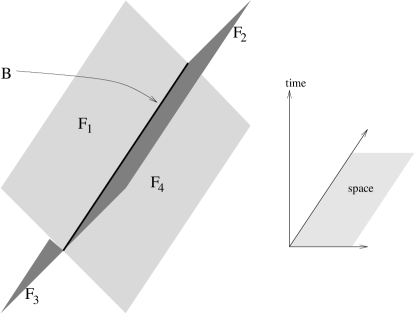
Figure 1: There are four families of light-rays projecting orthogonally away from a two-dimensional surface $B$, two future-directed families (one to each side of $B$) and two past-directed families. At least two of them will have non-positive expansion. The null hypersurfaces generated by non-expanding light-rays will be called “light-sheets.” The covariant entropy conjecture states that the entropy on any light-sheet cannot exceed a quarter of the area of $B$.

Which should we select? And how far may we follow the light-rays?

In order to construct a selection rule, let us briefly return to the limit in which Bekenstein’s bound applies. For a spherical surface around a Bekenstein system, the enclosed entropy cannot be larger than the area. But the same surface is also a boundary of the infinite region on its outside. The entropy outside could clearly be anything. From this we learn that it is important to consider the entropy only on hypersurfaces which are not outside the boundary.

But what does “outside” mean in general situations? The side that includes infinity? Then what if space is closed? Fortunately, there exists an intuitive notion of “inside” and “outside” that is suitable to be generalized to a covariant rule. Think of ordinary Euclidean geometry, and start from a closed surface $B$. Construct a second surface by moving every point on $B$ an infinitesimal distance away to one side of $B$, along lines orthogonal to $B$. If this increases the area, then we say that we have moved outside. If the area decreases, we have moved inside.

This consideration yields the selection rule. We start at $B$, and follow one of the four families of orthogonal light-rays, as long as the cross-sectional area is decreasing or constant. When it becomes increasing, we must stop. This can be formulated technically by demanding that the expansion of the orthogonal null congruence must be non-positive, in the direction away from the surface $B$. By continuity across $B$, the expansion of past-directed light-rays going to one side is the negative of the expansion of future-directed light-rays heading the other way. Therefore we can be sure that at least two of the four null directions will be allowed. If the expansion of one pair of null congruences vanishes on $B$, there will be three allowed directions. If the expansion of both pairs vanishes on $B$, all four null directions will be allowed.

This covariant definition of “inside” and “outside” does not require the surface $B$ to be closed. Only the naive definition, by which “inside” was understood to mean a finite region delimited by a surface, needed the surface to be closed. Therefore we shall now drop this condition and allow any connected two-dimensional surface. This enables us to assume without loss of generality that the expansion in each of the four null directions does not change sign anywhere on the surface $B$. If it does, we simply split $B$ into suitable domains and apply the entropy law to each domain individually.

Finally, in an attempt to protect our conjecture against pathologies such as superluminal entropy flow, we will require the dominant energy condition to hold: for all timelike $v_{a}$, $T^{ab}v_{a}v_{b}\geq 0$ and $T^{ab}v_{a}$ is a non-spacelike vector. This condition states that to any observer the local energy density appears non-negative and the speed of energy flow of matter is less than the speed of light. It implies that a space-time must remain empty if it is empty at one time and no matter is coming in from infinity [18]. It is believed that all physically reasonable forms of matter satisfy the dominant energy condition [18, 19], so we are not imposing a significant restriction. It may well be possible, however, to weaken the assumption further; this is under investigation.

We should also require that the space-time is inextendible and contains no null or timelike (“naked”) singularities. This is necessary if we wish to exclude the possibility of destroying or creating arbitrary amounts of entropy on such boundaries. These conditions are believed to hold in any physical space-time, so we shall not spell them out below. (Of course we are not excluding the spacelike singularities occuring in cosmology and in gravitational collapse; indeed, much of this paper will be devoted to investigating the validity of the proposed bound in the vicinity of such singularities.) We thus arrive at a conjecture for a covariant bound on the entropy in any space-time.

Covariant Entropy Conjecture

Let $M$ be a four-dimensional space-time on which Einstein’s equation is satisfied with the dominant energy condition holding for matter. Let $A$ be the area of a connected two-dimensional spatial surface $B$ contained in $M$. Let $L$ be a hypersurface bounded by $B$ and generated by one of the four null congruences orthogonal to $B$. Let $S$ be the total entropy contained on $L$. If the expansion of the congruence is non-positive (measured in the direction away from $B$) at every point on $L$, then $S\leq A/4$.

3 Discussion

3.1 The recipe

In the previous paragraph, we formulated the conjecture with an eye on formal accuracy and generality. For all practical purposes, however, it is more useful to translate it into a set of rules like the following recipe (see Fig. 1):

1. Pick any two-dimensional surface $B$ in the space-time $M$.

2. There will be four families of light-rays projecting orthogonally away from $B$ (unless $B$ is on a boundary of $M$): $F_{1}\ldots F_{4}$.

3. As shown in the previous section, we can assume without loss of generality that the expansion of $F_{1}$ has the same sign everywhere on $B$. If the expansion is positive (in the direction away from $B$), i.e., if the cross-sectional area is increasing, $F_{1}$ must not be used for an entropy/area comparison. If the expansion is zero or negative, $F_{1}$ will be allowed. Repeating this test for each family, one will be left with at least two allowed families. If the expansion is zero in some directions, there may be as many as three or four allowed families.

4. Pick one of the allowed families, $F_{i}$. Construct a null hypersurface $L_{i}$, by following each light-ray until one of the following happens:

   1. The light-ray reaches a boundary or a singularity of the space-time.

   2. The expansion becomes positive, i.e., the cross-sectional area spanned by the family begins to increase in a neighborhood of the light-ray.

   The hypersurface $L_{i}$ obtained by this procedure will be called a light-sheet of the surface $B$. For every allowed family, there will be a different light-sheet.

5. The conjecture states that the entropy $S_{i}$ on the light-sheet $L_{i}$ will not exceed a quarter of the area of $B$:

   $$S_{i}\leq\frac{A}{4}.$$ (3.1)

   Note that the bound applies to each light-sheet individually. Since $B$ may possess up to four light-sheets, the total entropy on all light-sheets could add up to as much as $A$.

We should add some remarks on points 2 and 3. In many situations it will be natural to call $F_{1}\ldots F_{4}$ the future-directed ingoing, future-directed outgoing, past-directed ingoing and past-directed outgoing family of surface-orthogonal geodesics. But we stress that “ingoing” and “outgoing” are just arbitrary labels distinguishing the two sides of $B$; only if $B$ is closed, there might be a preferred way to assign these names. Our rule does not refer to “ingoing” and “outgoing” explicitly.

In fact the covariant entropy bound does not even refer to “future” and “past.” The conjecture is manifestly time reversal invariant. We regard this as its most significant property. After all, thermodynamic entropy is never T-invariant, and neither is the generalized second law of thermodynamics, which underlies Bekenstein’s bound. This will be discussed further in Sec. 3.4. One can draw strong conclusions from these simple observations (Sec. 7).

If $B$ is a closed surface, we can characterize it as trapped, anti-trapped or normal (see Refs. [18, 19] for definitions). This provides a simple criterion for the allowed families. If $B$ is trapped (anti-trapped), it has two future-directed (past-directed) light-sheets. If $B$ is normal, it has a future-directed and a past-directed light-sheet on the same side, which is usually called the inside. If $B$ lies on an apparent horizon (the boundary between a trapped or anti-trapped region and a normal region), it can have more than two light-sheets. For example, if $B$ is marginally outer trapped [18], i.e., if the future-directed outgoing geodesics have zero convergence, then it has two future-directed light-sheets and a past-directed ingoing light-sheet.

3.2 Caustics as light-sheet endpoints

We have defined a light-sheet to be a certain subset of the null hypersurface generated by an “allowed” family of light-rays. The rule is to start at the surface $B$ and to follow the light-rays only as long as the expansion is zero or negative. In order to understand if and why the conjecture may be true, we must understand perfectly well what it is that can cause the expansion to become positive. After all, it is this condition alone which must prevent the light-sheet from sampling too much entropy and violating the conjectured bound. Our conclusion will be that the expansion becomes positive only at caustics. The simplest example of such a point is the center of a sphere in Minkowski space, at which all ingoing light-rays intersect.

Raychauduri’s equation for a congruence of null geodesics with tangent vector field $k^{a}$ and affine parameter $\lambda$ is given by

$$\frac{d\theta}{d\lambda}=-\frac{1}{2}\theta^{2}-\hat{\sigma}_{ab}\hat{\sigma}^{ab}-8\pi T_{ab}k^{a}k^{b}+\hat{\omega}_{ab}\hat{\omega}^{ab},$$ (3.2)

where $T_{ab}$ is the stress-energy tensor of matter. The expansion $\theta$ measures the local rate of change of an element of cross-sectional area ${\cal A}$ spanned by nearby geodesics:

$$\theta=\frac{1}{\cal A}\frac{d\cal A}{d\lambda}.$$ (3.3)

The vorticity $\hat{\omega}_{ab}$ and shear $\hat{\sigma}_{ab}$ are defined in Refs. [18, 19]. The vorticity vanishes for surface-orthogonal null congruences. The first and second term on the right hand side are manifestly non-positive. The third term will be non-positive if the null convergence condition [18] holds:

$$T_{ab}k^{a}k^{b}\geq 0~{}~{}\mbox{for all null}~{}k^{a}.$$ (3.4)

The dominant energy condition, which we are assuming, implies that the null convergence condition will hold. (It is also implied by the weak energy condition, or by the strong energy condition.)

Therefore the right hand side of Eq. (3.2) is non-positive. It follows that $\theta$ cannot increase along any geodesic. (This statement is self-consistent, since the sign of $\theta$ changes if we follow the geodesic in the opposite direction.) Then how can the expansion ever become positive? By dropping two of the non-positive terms in Eq. (3.2), one obtains the inequality

$$\frac{d\theta}{d\lambda}\leq-\frac{1}{2}\theta^{2}.$$ (3.5)

If the expansion takes the negative value $\theta_{0}$ at any point on a geodesic in the congruence, Eq. (3.5) implies that the expansion will become negative infinite, $\theta\rightarrow-\infty$, along that geodesic within affine time $\Delta\lambda\leq 2/|\theta_{0}|$ [19]. This can be interpreted as a caustic. Nearby geodesics are converging to a single focal point, where the cross-sectional area $\cal A$ vanishes. When they re-emerge, the cross-sectional area starts to increase. Thus, the expansion $\theta$ jumps from $-\infty$ to $+\infty$ at a caustic. Then the expansion is positive, and we must stop following the light-ray. This is why caustics form the endpoints of the light-sheet.

3.3 Light-sheet examples and first evidence

The considerations in Sec. 3.2 allow us to rephrase the rule for constructing light-sheets: Follow each light-ray in an allowed family until a caustic is reached. The effect of this prescription can be understood by thinking about closed surfaces in Minkowski space. The simplest example is a spherical surface. The past-directed outgoing and future-directed outgoing families are forbidden, because they have positive expansion. The past- and future-directed ingoing families are allowed. Both encounter caustics when they reach the center of the sphere. Thus they each sweep the interior of the sphere exactly once. If we deform the surface into a more irregular shape, such as an ellipsoid, there may be a line, or even a surface, of caustics at which the light-sheet ends. In some cases (e.g. if the surface is a box and does not enclose much matter), non-neighbouring light-rays may cross. This does not constitute a caustic, and the light-rays need not be terminated there. They can go on until they are bent into caustics by the matter they encounter. Thus some of the entropy may be counted more than once. This is merely a consequence of a desirable feature of our prescription: that it is local and applies separately to every infinitesimal part of any surface.

For a spherical surface surrounding a spherically symmetric body of matter, the ingoing light-rays will end on a caustic in the center, as for an empty sphere. If the interior mass distribution is not spherically symmetric, however, some light-rays will be deflected into angular directions, and will form “angular caustics” (see Fig. 2).

Figure 2: Light-rays from a spherical surface into a massive body. If the body is spherically symmetric internally (left), the light-rays all meet at a “radial” caustic in the center of the sphere. If the internal mass distribution is not spherically symmetric, most rays get deflected into angular directions and end on “angular caustics.” The picture on the right shows an example with four overdense regions. The thick lines represent caustics.

This does not mean that the interior will not be completely swept out by the light-sheet. Between two light-rays that get deflected into different overdense regions, there are infinitely many light-rays that proceed further inward. It does mean, however, that we have to follow some of the light-rays for a much longer affine time than we would in the spherically symmetric case.

This does not make a difference for static systems: they will be completely penetrated by the light-sheet in any case. In a system undergoing gravitational collapse, however, light-rays will hit the future singularity after a finite affine time. Consider a collapsing ball which is exactly spherically symmetric, and a future-ingoing light-sheet starting at the outer surface of the system, when it is already within its own Schwarzschild horizon. We can arrange things so that the light-sheet reaches the caustic at $r=0$ exactly when it also meets the singularity (see Fig. 3).

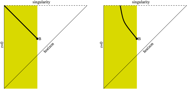
Figure 3: Two Penrose diagrams for collapsing spherical objects of identical mass. Each point represents a two-sphere. The thick lines are light-rays. In an object which is spherically symmetric internally (left), the future-directed ingoing light-rays originating from its surface $B$ (at a suitable time) just make it to the center of the object before reaching the singularity. In a highly disordered system, on the other hand, light-rays will be deflected into angular directions (right). We are taking the surface $B$ to have the same area as before. The light-ray path looks timelike because the angular directions are suppressed in the diagram. We see that the light-rays will not sweep the entire interior of the disordered system before meeting the singularity.

Now consider a different collapsing ball, of identical mass, and identical radius when the light-rays commence. While this ball may be spherically symmetric on the large scale, let us assume that it is highly disordered internally. The light-rays will thus be deflected into angular directions. As Fig. 2 illustrates, this means that they take intricate, long-winded paths through the interior: they “percolate.” This consumes more affine time than the direct path to the center taken in the first system. Therefore the second system will not be swept out completely before the singularity is reached (see Fig. 3).

Why did we spend so much time on this example? The first ball is a system with low entropy, while the second ball has high entropy. One might think that no kind of entropy bound can apply when a highly enthropic system collapses: the surface area goes to zero, but the entropy cannot decrease. The above considerations have shown, however, that light-sheets percolate rather slowly through highly enthropic systems, because the geodesics follow a kind of random walk. Since they end on the black hole singularity within finite affine time, they sample a smaller portion of a highly enthropic system than they would for a more regular system. (In Fig. 2, the few light-rays that go straight to the center of the inhomogeneous system also take more affine time to do so than in a homogeneous system, because they pass through an underdense region. In a homogeneous system, they would encounter more mass; by Raychauduri’s equation, this would accelerate their collapse.) Therefore it is in fact quite plausible, if counter-intuitive, that the covariant entropy bound holds even during the gravitational collapse of a system initially saturating Bekenstein’s bound.

In Sec. 6, we will discuss additional constraints on the penetration depth of light-sheets in collapsing highly enthropic systems, and a quantitative test will be performed.

3.4 Recovering Bekenstein’s bound

The covariant entropy conjecture can only be sensible if we can recover Bekenstein’s bound from it in an appropriate limit. For a Bekenstein system (see Sec. 1.1: a thermodynamic system of constant, finite size and limited self-gravity), the boundary area should bound the entropy in the spatial region occupied by the system. The covariant bound, on the other hand, uses null hypersurfaces to compare entropy and area. Then how can Bekenstein’s bound be recovered?

While null hypersurfaces are certainly required in general, it turns out that there is a wide class of situations in which an entropy bound on spacelike hypersurfaces can be inferred from the covariant entropy conjecture. We will now identify sufficient conditions and derive a theorem on the entropy of spatial regions. We will then show that Bekenstein’s entropy/area bound is indeed implied by the covariant bound, namely as a special case of the theorem.

Let $A$ be the area of a closed surface $B$ possessing at least one future-directed light-sheet $L$. Suppose that $L$ has no boundary other than $B$. Then we shall call the direction of this light-sheet the “inside” of $B$. Let the spatial region $V$ be the interior of $B$ on some spacelike hypersurface through $B$. If the region $V$ is contained in the causal past of the light-sheet $L$, the dominant energy condition implies that all matter in the region $V$ must eventually pass through the light-sheet $L$. Then the second law of thermodynamics implies that the entropy on $V$, $S_{V}$, cannot exceed the entropy on $L$, $S_{L}$. By the covariant entropy bound, $S_{L}\leq A/4$. It follows that the entropy of the spatial region $V$ cannot exceed a quarter of its boundary area: $S_{V}\leq A/4$.

The condition that the future-directed light-sheet $L$ contain no boundaries makes sure that none of the entropy of the spatial region $V$ escapes through holes in $L$. Neither can any of the entropy escape into a black hole singularity, because we have required that the spatial region must lie in the causal past of $L$. Since we are always assuming that the space-time is inextendible and that no naked singularities are present, all entropy on $V$ must go through $L$. We summarize this argument in the following theorem.

Spacelike Projection Theorem

Let $A$ be the area of a closed surface $B$ possessing a future-directed light-sheet $L$ with no boundary other than $B$. Let the spatial region $V$ be contained in the intersection of the causal past of $L$ with any spacelike hypersurface containing $B$. Let $S$ be the entropy on $V$. Then $S\leq A/4$.

Now consider, in asymptotically flat space, a Bekenstein system in a spatial region $V$ bounded by a closed surface $B$ of area $A$. The future-directed ingoing light-sheet $L$ of $B$ exists (otherwise $B$ would not have “limited self-gravity”), and can be taken to end whenever two (not necessarily neighbouring) light-rays meet. Thus it will have no other boundary than $B$. Since the gravitational binding of a Bekenstein system is not strong enough to form a black hole, $V$ will be contained in the causal past of $L$. Therefore the conditions of the theorem are satisfied, and the entropy of the system must be less than $A/4$. We have recovered Bekenstein’s bound.

There are many other interesting applications of the theorem. In particular, it can be used to show that area bounds entropy on spacelike sections of anti-de Sitter space. This can be seen by taking $B$ to be any sphere, at any given time. The future-ingoing light-sheet of $B$ exists, and unless the space contains a black hole, has no other boundary. Its causal past includes the entire space enclosed by $B$. This remains true for arbitrarily large spheres, and in the limit as $B$ approaches the boundary at spatial infinity.

The theorem is immensely useful, because it essentially tells us under which conditions we can treat a region of space as a Bekenstein system. In general, however, the light-sheets prescribed by the covariant entropy bound provide the only consistent way of comparing entropy and area.

We pointed out in Sec. 3.1 that the covariant entropy bound is T-invariant. The spacelike projection theorem is not T-invariant; it refers to past and future explicitly. This is because the second law of thermodynamics enters its derivation. The asymmetry is not surprising, since Bekenstein’s bound, which we recovered by the theorem, rests on the second law. We should be surprised only when an entropy law is T-invariant. It is this property which forces us to conclude that the origin of the covariant bound is not thermodynamic, but statistical (Sec. 7).

4 Cosmological tests

The simplest way to falsify the conjecture would be to show that it conflicts directly with observation. In this section, we will apply the covariant bound to the cosmological models that our universe is believed to be described by (and to many more by which it certainly is not described). Since we claim that the conjecture is a universal law valid for all space-times satisfying Einstein’s equations (with the dominant energy condition holding for matter), it must be valid for cosmological solutions in particular. We will see that it passes the test, and more significantly, it just passes it.

We consider Friedmann-Robertson-Walker (FRW) cosmologies, which are described by a metric of the form

$$ds^{2}=-dt^{2}+a^{2}(t)\left(\frac{dr^{2}}{1-kr^{2}}+r^{2}d\Omega^{2}\right).$$ (4.1)

An alternative form uses comoving coordinates:

$$ds^{2}=a^{2}(\eta)\left[-d\eta^{2}+d\chi^{2}+f^{2}(\chi)d\Omega^{2}\right].$$ (4.2)

Here $k=-1$, $0$, $1$ and $f(\chi)=\sinh\chi$, $\chi$, $\sin\chi$ correspond to open, flat, and closed universes respectively.

The Hubble horizon is the inverse of the expansion rate $H$:

$$r_{\rm HH}=H^{-1}=\frac{a}{da/dt}.$$ (4.3)

The particle horizon is the distance travelled by light since the big bang:

$$\chi_{\rm PH}=\eta.$$ (4.4)

The apparent horizon is defined geometrically as a sphere at which at least one pair of orthogonal null congruences have zero expansion. It is given by [14]

$$r_{\rm AH}=\frac{1}{\sqrt{H^{2}+\frac{k}{a^{2}}}}.$$ (4.5)

Using Friedmann’s equation,

$$H^{2}=\frac{8\pi\rho}{3}-\frac{k}{a^{2}},$$ (4.6)

one finds

$$r_{\rm AH}=\sqrt{\frac{3}{8\pi\rho}},$$ (4.7)

where $\rho$ is the energy density of matter.

We consider matter described by $T_{ab}=\mbox{diag}(\rho,p,p,p)$, with pressure $p=\gamma\rho$. The dominant energy condition requires that $\rho\geq 0$ and $-1\leq\gamma\leq 1$. The case $\gamma=-1$ is special, because it leads to a different global structure from the other solutions. It corresponds to de Sitter space, which has no past or future singularity. This solution is significant because it describes an inflationary universe. We will comment on inflation at the end of Sec. 4.1.

We will test the conjecture on spherical surfaces $B$ characterized by some value of $r$, or of $(\eta,\chi)$. As we found at the end of Sec. 3.1, the directions of the light-sheets of a surface depend on its classification as trapped, normal, or anti-trapped. In the vicinity of $\chi=0$ (and for closed universes, also on the opposite pole, near $\chi=\pi$), the spherical surfaces will be normal. The larger spheres beyond the apparent horizon(s) will be anti-trapped. Some universes, for example most closed universes, or a flat universe with negative cosmological constant [15], recollapse. Such universes necessarily contain trapped surfaces. But trapped regions can occur in any case by gravitational collapse. The surfaces in the interior of such regions provide a serious challenge for the covariant entropy conjecture, because their area shrinks to zero while the enclosed entropy cannot decrease. We address this problem in some generality in Sec. 6, where we argue that the conjecture holds even in such regions. Because of its importance, the special case of the adiabatic recollapse of a closed universe will be treated explicitly in Sec. 5.2. In the present section, we shall therefore discuss only normal and anti-trapped surfaces.

4.1 Anti-trapped surfaces

An anti-trapped surface $B$ contains two past-directed light-sheets. Unless $B$ lies within the particle horizon (of either pole in the closed case), both light-sheets will be “truncated” at the Planck era near the past singularity. The truncation has the desirable effect that the volume swept by the light-sheets grows not like $A^{3/2}$, but roughly like the area. In fact, the “ingoing” light-sheet coincides with the “truncated lightcones” used in the entropy conjecture of Fischler and Susskind [9], and the other light-sheet can be treated similarly. In open universes the bound will be satisfied more comfortably than in flat ones [9]. The validity of the bound was checked for flat universes with $0\leq\gamma\leq 1$ in Ref. [9] and for $-1<\gamma<0$ in Ref. [15]. Here we will give a summary of these results, and we will explain why reheating after inflation does not violate the covariant bound. Subtleties arising in closed universes will be discussed separately in Sec. 5.2.

The reason why the bound is satisfied near a past singularity is simple. The first moment of time that one can sensibly talk about is one Planck time after the singularity. At this time, there cannot have been more than one unit of entropy per Planck volume, up to a factor of order one. This argument does not involve any assumptions about “holography;” we are merely applying the usual Planck scale cutoff. We cannot continue light-sheets into regions where we have no control over the physics. A backward light-sheet of an area $A$ specified at $t=2t_{\rm Pl}$ will be truncated at $t=t_{\rm Pl}$. It will sweep a volume of order $Al_{\rm Pl}$ and the entropy bound will at most be saturated.

Let us define $\sigma$ as the entropy/area ratio at the Planck time. Consider a universe filled with any type of matter allowed by the dominant energy condition, $-1\leq\gamma\leq 1$. We may exclude $\gamma=-1$, since de Sitter space does not contain a singularity in the past. The scale factor will be given by $a(t)=t^{\frac{2}{3(\gamma+1)}}$. If the evolution is adiabatic, the ratio of entropy to area behaves as [15]

$$\frac{S}{A}\leq\sigma t^{\frac{\gamma-1}{\gamma+1}}$$ (4.8)

for any past-directed light-sheet of areas specified at a later time $t$. (Equality holds, e.g., for spherical areas at least as large as the particle horizon.) The exponent is non-positive, so the entropy/area ratio does not increase. Since the bound is satisfied at the Planck time, it will remain satisfied later.

Another way to see this is to consider the particle horizon $n$ (e.g. $n=10$) Planck times after the big bang of a flat FRW universe. Its area will be $O(n^{2})$ and its past-directed light-sheet will sweep $O(n^{3})$ Planck volumes. Let us assume that each of these Planck volumes contains one unit of entropy; then the bound would be violated. But most of these volumes are met by the light-sheet at a time later than $t_{\rm Pl}$. Therefore there must have been, at the Planck time, Planck volumes containing more than a unit of entropy, which is impossible. (Note that this argument would break down if we allowed naked singularities!)

If the evolution is non-adiabatic, the entropy bound nevertheless predicts that $S/A\leq 1/4$, implying that there is a limit on how rapidly the universe can produce entropy. This will be further discussed in Sec. 4.2.

Inflation

Of course the notion that the standard cosmology extends all the way back to the Planck era is not seriously tenable. In order to understand essential properties of our universe, such as its homogeneity and flatness, and its perturbation spectrum, it is usually assumed that the radiation dominated era was preceded by a vacuum dominated era.

Inflation ends on a spacelike hypersurface $V$ at $t=t_{\rm reheat}$. At this time, all the entropy in the universe is produced through reheating. Both before and after reheating, all spheres will be anti-trapped except in a small neighbourhood of $r=0$ (or small neighbourhoods of the poles of the $S^{3}$ spacelike slice in a closed universe), of the size of the apparent horizon. Therefore the spacelike projection theorem does not apply to any but the smallest of the surfaces $B\subset V$. The other spheres may be exponentially large, but the covariant conjecture does not relate their area to the enclosed entropy. The size and total entropy of the reheating hypersurface $V$ is thus irrelevant.

Outside the apparent horizon, entropy/area comparisons can only be done on the light-sheets specified in the conjecture. Indeed, the past-directed light-sheets of anti-trapped surfaces of the post-inflationary universe do intersect $V$. Since there is virtually no entropy during inflation, we can consider the light-sheets to be truncated by the reheating surface. Because inflation cannot produce more than one unit of entropy per Planck volume, the bound will be satisfied by the same arguments that were given above for universes with a big bang.

4.2 Normal surfaces

Spatial regions enclosed by normal surfaces will turn out, in a sense specified below, to be analogues to “Bekenstein systems” (see Sec. 1.1). In order to understand this, we must establish a few properties of Bekenstein systems. For quick reference, we will call the first bound, Eq. (1.1), Bekenstein’s entropy/mass bound, and the second bound, Eq. (1.3), Bekenstein’s entropy/area bound. For a spherical Bekenstein system of a given radius and mass, the entropy/mass bound is always at least as tight as the entropy/area bound. This because a Bekenstein system must be gravitationally stable ($M\leq R/2$), which implies $2\pi RM\leq\pi R^{2}=A/4$. A spherical system that saturates Bekenstein’s entropy/area bound will be called a saturated Bekenstein system. The considerations above imply that this system will also saturate the entropy/mass bound. In semi-classical gravity, a black hole, viewed from the outside, is an example of a saturated Bekenstein system; but for many purposes it is simpler to think of an ordinary, maximally enthropic, spherical thermodynamic system just on the verge of gravitational collapse. A system that saturates the entropy/mass bound but not the entropy/area bound will be called a mass-saturated Bekenstein system. If we find a spherical thermodynamic system which saturates the entropy/area bound but does not saturate the entropy/mass bound, we must conclude that it was not a Bekenstein system in the first place.

The normal region contains a past- and a future-directed light-sheet. Both of them are ingoing, i.e. they are directed towards the center of the region at $\chi=0$ (or $\chi=\pi$ for the normal region near the opposite pole in closed universes). This is crucial. If outgoing light-sheets existed even as $\chi\rightarrow 0$, the area would become arbitrarily small while the entropy remained finite. This is one of the reasons why the Fischler-Susskind proposal does not apply to closed universes (see Sec. 5.2). Except for this constraint, the past-directed light-sheet coincides with the light-cones used by Fischler and Susskind. The entropy/area bound has been shown to hold on such surfaces [9, 14, 15]. We will therefore consider only the future-directed light-sheet.

The future-directed light-sheet covers the same comoving volume as the past light-sheet. Therefore the covariant entropy bound will be satisfied on it if the evolution is adiabatic. But we certainly must allow the possibility that additional entropy is produced. Consider, for example, the outermost surface on which future-directed light-sheets are still allowed, a sphere $B$ on the apparent horizon. Suppose that an overfunded group of experimental cosmologists within the apparent horizon are bent on breaking the entropy bound. They must try to produce as much entropy as possible before the matter passes through the future-directed light-sheet $L$ of $B$. What is their best strategy?

Note that they cannot collect any mass from outside $B$, because $L$ is a null hypersurface bounded by $B$ and the dominant energy condition holds, preventing spacelike energy flow. The most enthropic system is a saturated Bekenstein system, so they should convert all the matter into such systems. (As discussed above, saturated Bekenstein systems are just on the verge of gravitational collapse and contain the same amount of entropy as a black hole of the same mass and radius. By using ordinary thermodynamic systems instead of black holes, one ensures that the light-sheet actually permeates the systems completely and samples all the entropy, rather than being truncated by the black hole singularity; see Secs. 3.3 and 6 for a discussion of these issues.)

If all matter is condensed into several small highly enthropic systems, they will be widely separated, i.e. surrounded by empty regions of space which are large, flat, and static compared to the length scale of any individual system. By the dominant energy condition, no negative energy is present. Therefore conditions given in Sec. 1.1 are fulfilled. We are thus justified in applying Bekenstein’s bounds to the systems, and we should use the entropy/mass bound, Eq. (1.1), because it is tighter. In order to create the maximum amount of entropy, however, it is best to put the matter into a few large saturated Bekenstein systems, rather than many small ones. Therefore we should take the limit of a Bekenstein system, as large as the apparent horizon and containing the entire mass within it. Of course the question arises whether the calculation remains consistent in this limit, both in its treatment of the interior as a Bekenstein system, and in its evaluation of the mass. We will show below, purely from the point of view of Bekenstein’s bound, that the interior of the apparent horizon is in fact the largest system for which Bekenstein’s conditions can be considered to hold; for larger systems, inconsistencies arise. In Sec. 5.3, we will use the spacelike projection theorem to arrive at the same conclusion within the framework of the covariant entropy conjecture.

We have cautioned in Sec. 2 against using an entropy/mass bound in general space-times, because there is no concept of local energy density. In this case, however, the mass is certainly well defined before we take the limit of a single Bekenstein system, because the many saturated systems will be widely separated and can be treated as immersed in asymptotically flat space. In the limit of a single system, we can follow Ref. [14] and treat the interior of the apparent horizon as part of an oversized spherical star. (We are thus pretending that somewhere beyond the apparent horizon, the space-time may become asymptotically flat and empty. This is not an inconsistent assumption as long as Bekenstein’s conditions are satisfied; we show below that this is indeed the case. Related ideas, not referring specifically to the apparent horizon, underly some proposals for cosmological entropy bounds given in Refs. [12, 13, 15].) Then we can apply the usual mass definition for spherically symmetric systems [20] to the interior region.

The circumferential radius of our system is the apparent horizon radius, and is given by Eq. (4.7):

$$r_{\rm AH}=\sqrt{\frac{3}{8\pi\rho}}.$$ (4.9)

The mass inside the apparent horizon is given by [20]

$$M(r_{\rm AH})=\int_{0}^{r_{\rm AH}}4\pi r^{2}\rho dr=\frac{4\pi}{3}r_{\rm AH}^{3}\rho.$$ (4.10)

This yields $r_{\rm AH}=2M(r_{\rm AH})$. By Bekenstein’s entropy/mass bound, Eq. (1.1), the entropy cannot exceed $2\pi M(r_{\rm AH})\,r_{\rm AH}$. Thus we find

$$S_{\rm max}=\pi r_{\rm AH}^{2}.$$ (4.11)

This is exactly a quarter of the area of the apparent horizon.

Eq. (4.7) follows from the Friedmann equation (which involves only the density but not the pressure), and from Eq. (4.5), which is a geometric property of the FRW metrics. Thus the calculation holds independently of the equation of state. We have not dropped any factors of order one, and attained exactly the saturation of the bound. This would not be the case for the Hubble horizon or the particle horizon. We conclude that the entropy on the future-directed light-sheet $L$ will not exceed a quarter of the area of the boundary $B$. The covariant entropy bound may be saturated on the apparent horizon, but it will not be violated, no matter how hard we try to produce entropy.

The property $r=2M(r)$ is special to the apparent horizon. It suggests that we should consider the interior of the apparent horizon to be the largest region with non-dominant self-gravity, and thus the largest system to which Bekenstein’s bound can be applied. This statement can be made more precise. The property $r_{\rm AH}=2M(r_{\rm AH})$ means that if we treat the interior as a Bekenstein system, it can be saturated, not just mass-saturated (see page 4.2 for definitions). If we chose a smaller surface $r_{X}<r_{\rm AH}$, the enclosed mass would be less than half of the radius, $2M<r_{X}$. In this case, (area-)saturation would not be possible, but only mass-saturation. This is because the entropy/mass bound yields $2\pi Mr_{X}<\pi r_{X}^{2}=A/4$. We conclude that the covariant entropy bound, which uses area, cannot be saturated on such surfaces. On the other hand, surfaces outside the apparent horizon, $r_{X}>r_{\rm AH}$, possess no future-directed light-sheet to which we could apply the covariant bound. We find this reflected in the property $2M>r_{X}$ for such surfaces. It implies that one could build a mass-saturated spherical system which breaks Bekenstein’s entropy/area bound: $2\pi Mr_{X}>\pi r_{X}^{2}$. As we discussed at the beginning of this subsection, this indicates a breakdown of the treatment of the enclosed region as a Bekenstein system. It follows that the apparent horizon is the largest sphere whose interior may be treated as a Bekenstein system. For larger systems, Bekenstein’s assumptions would not be self-consistent.

From the point of view of the covariant entropy conjecture, there are well-defined sufficient conditions for the treatment of a spatial region as a Bekenstein system, namely those spelled out in the spacelike projection theorem (Sec. 3.4). This will be applied to cosmology in the Sec. 5.1. We will show formally that the region inside the apparent horizon is indeed the largest region for which Bekenstein’s entropy/area bound may be guaranteed to hold, if certain additional conditions are met.

5 Cosmological entropy bounds

5.1 A cosmological corollary

In Sec. 4.2, we tested the covariant entropy conjecture on future-directed light-sheets in normal regions, by assuming maximal entropy production in the interior spatial region. We found that the bound may be saturated, but not violated. We will now switch viewpoints, assume that the covariant entropy conjecture is a correct law, and derive an entropy bound for spatial regions in cosmology.

Normal regions offer an interesting application of the spacelike projection theorem (Sec. 3.4). It tells us under which conditions we can treat the interior of the apparent horizon as a Bekenstein system. Let $A$ be the area of a sphere $B$, on or inside of the apparent horizon. (“Inside” has a natural meaning in normal regions.) Then the future-directed ingoing light-sheet $L$ exists. Let us assume that it is complete, i.e., $B$ is its only boundary. (This condition is fulfilled, e.g., for any radiation or dust dominated FRW universe with no cosmological constant.) Let $V$ be a region inside of and bounded by $B$, on any spacelike hypersurface containing $B$. If no black holes are produced, $V$ will be in the causal past of $L$, and the conditions for the spacelike projection theorem are satisfied. Therefore, the entropy on $V$ will not exceed $A/4$. In particular, we may choose $B$ to be on the apparent horizon, and $V$ to be on the spacelike slice preferred by the homogeneity of the FRW cosmologies. We summarize these considerations in the following corollary:

Cosmological Corollary

Let $V$ be a spatial region within the apparent horizon of an observer. If the future-directed ingoing light-sheet $L$ of the apparent horizon has no other boundaries, and if $V$ is entirely contained in the causal past of $L$, then the entropy on $V$ cannot exceed a quarter of the area of the apparent horizon.

By definition, the spheres beyond the apparent horizon are anti-trapped and possess no future-directed light-sheets. Therefore the spacelike projection theorem does not apply, and no statement about the entropy enclosed in spatial volumes can be made. (Of course, we can still use their area to bound the entropy on their light-sheets.) Thus the covariant entropy conjecture singles out the apparent horizon as a special surface. It marks the largest surface to which the spacelike projection theorem can possibly apply, and hence the region inside it is the largest region one can hope to treat as a Bekenstein system. This conclusion agrees with the result obtained in the previous subsection from a consistency analysis of Bekenstein’s assumptions for regions larger than the apparent horizon.

As an example, the conditions of this corollary are satisfied by the apparent horizon of de Sitter space. It coincides with the cosmological horizon, at $r=(3/\Lambda)^{1/2}$. Thus the entropy within the cosmological horizon cannot exceed $3\pi/\Lambda$. The corollary will be further applied in Sec. 5.3.

The corollary tells us if and how Bekenstein’s bound can be applied to spatial regions in cosmological solutions. It follows from, but is not equivalent to, the covariant entropy bound. Like the spacelike projection theorem, the corollary is a statement of limited scope. It contains no information how to relate entropy to the area of trapped or anti-trapped surfaces in the universe, and even for surfaces within the apparent horizon, a “spacelike” bound applies only under certain conditions. Thus, the role of the corollary is to define the range of validity of Bekenstein’s entropy/area bound in cosmological solutions. Precisely for this reason, the corollary is far less general than the covariant conjecture, which associates at least two hypersurfaces with any surface in any space-time, and bounds the entropy on those hypersurfaces.

5.2 The Fischler-Susskind bound

Among the recently proposed cosmological entropy bounds [9, 12, 13, 14, 15, 16], the prescription of Fischler and Susskind (FS) is distinct in that it attempts to relate entropy to every spherical surface in the universe, namely the entropy on the past-directed “ingoing” null hypersurface. The covariant entropy conjecture is very much in this spirit; but we have changed the prescription from “past-ingoing” to a general selection rule determining at least two light-sheets on which entropy can be compared to area. The FS hypersurface will often be one of them, but not always. The limitations of the FS proposal can be understood in terms of this selection rule.

Consider the entropy on the null hypersurface formed by the particle horizon, emanating from the South pole in a closed, adiabatic, dust-dominated FRW universe [9]. The solution is given by

$$a(\eta)=\frac{a_{\rm max}}{2}(1-\cos\eta),~{}~{}~{}t(\eta)=\frac{a_{\rm max}}{2}(\eta-\sin\eta).$$ (5.1)

The entropy may not exceed one per Planck volume at the Planck time, $\eta_{\rm Pl}\sim a_{\rm max}^{-1/3}$. Therefore the total entropy of the universe will not be larger than $S_{\rm max}\sim a(\eta_{\rm Pl})^{3}\sim a_{\rm max}$.

The particle horizon has $\eta=\chi$, while the apparent horizon is given by $\eta=2\chi$ (see Fig. 4).

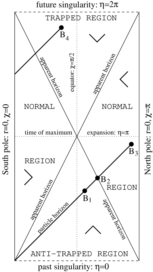
Figure 4: Penrose diagram for a closed FRW universe dominated by dust. The horizontal lines correspond to $S^{3}$ spacelike sections. Every point represents a two-sphere. The apparent horizons divide the space-time into four regions. The directions of light-sheets in each region are indicated by small wedges.

Thus the particle horizon will initially be outside the apparent horizon, in an anti-trapped region. Any surfaces met by the particle horizon in this region (such as $B_{1}$) possess a past-directed light-sheet that coincides with the particle horizon. Therefore the FS bound and the covariant bound should both be satisfied. Before the time of maximum expansion ($\eta=\pi$), the particle horizon reaches the sphere $B_{2}$ at $\eta=\chi=2\pi/3$. Let us verify explicitly that the bounds are still satisfied there. At this time, the particle horizon covers two-thirds of the total entropy of the universe, which will be of order $a_{\rm max}$. Its area, however, is $4\pi(3/4)^{3}a_{\rm max}^{2}$, which is much larger.

For $\eta=\chi>2\pi/3$ the particle horizon ends on normal, rather than anti-trapped spheres. It has entered a normal region surrounding the North pole and bounded by a different apparent horizon, $\eta=2(\pi-\chi)$. The surfaces in this region contain a future- and a past-directed light-sheet, both pointing towards the North pole. The particle horizon, which goes to the South pole, is now one of the “forbidden” families of light-rays (Sec. 3.1). According to the covariant bound, the entropy contained on it has nothing to do with the surface that bounds it. Indeed, its area approaches zero when it encompasses nearly the entire entropy of the universe ($B_{3}$). The FS bound cannot be applied here. It would continue to compare entropy and area of the particle horizon, and would be violated [9].

In Sec. 2, the selection rule was motivated by the requirement that one should compare the area of a surface only to the entropy that is, in some sense, inside of it, not outside. This consideration is paying off here. The spheres very close to the North pole, like any other $S^{2}$ on an $S^{3}$, enclose two regions. Because the region including the North pole is much smaller than the region including the South pole, one would like to call the former the “inside” and the latter the “outside.” The selection rule turns this intuitive notion into a covariant definition, which takes into account not only the shape of space but also its dynamics. Trapped surfaces, for example, have light-sheets on both sides, but only future-directed ones. This makes sense because in a collapsing region, loosely speaking, the direction in which surfaces are getting smaller is the future.

Returning to the example of a closed, adiabatic, dust-dominated FRW universe, consider a surface $B_{4}$ in the trapped region, near the equator of the $S^{3}$ spacelike surfaces (see Fig. 4). By choosing $B_{4}$ to be very close to the future singularity, its area can be made arbitrarily small. The FS hypersurface would go to the past and would pick up nearly half of the total entropy, so the FS bound cannot be used in this region. The covariant bound remains valid, because it applies only to the future-directed null hypersurfaces, which are soon truncated by the singularity.

5.3 Other cosmological entropy bounds

Other proposals for cosmological entropy bounds [12, 13, 14, 15, 16] are based on the idea of defining a limited spatial region to which Bekenstein’s bound can be applied. The definitions refer variously to the Hubble horizon (or to a region of size $\sim H^{-1}=a/\dot{a}$) [12, 13, 15, 16], a region of size $\sim t$ [15], and, remarkably, the apparent horizon [14]. In its simplified version, the Fischler-Susskind proposal can be included in this class, as referring to the region within the particle horizon [9].

The prescriptions do not aim to relate entropy to any surfaces larger than the specified ken. Also, most do not claim validity during the collapsing era of a closed universe, and none can be applied in arbitrary gravitationally collapsing systems. The covariant entropy bound differs from this approach in that it attempts generality: It associates hypersurfaces with any surface in any space-time and bounds the entropy contained on those hypersurfaces.

The proposed cosmological bounds are very useful for estimating the maximal entropy in limited regions of cosmological solutions. Even if a horizon other than the apparent horizon is used, one may still obtain correct results at least within factors of order one. In order to avoid pitfalls, however, they must be used carefully (as many authors have stressed). The corollary derived in Sec. 5.1 contains precise conditions determining whether, and to which regions of the universe, Bekenstein’s bound can be applied.

Consider, for example, the bound of Bak and Rey [14], which refers explicitly to the spatial region within the apparent horizon. One might be tempted to consider this as a special case of the covariant entropy bound, in the sense of the corollary derived in Sec. 5.1. Then it should always be valid. But Kaloper and Linde [15] have shown that this bound is exceeded in flat, adiabatic FRW universes with an arbitrarily small but non-vanishing negative cosmological constant. So what has gone wrong?

As the Penrose diagram for this space-time (Fig. 5)

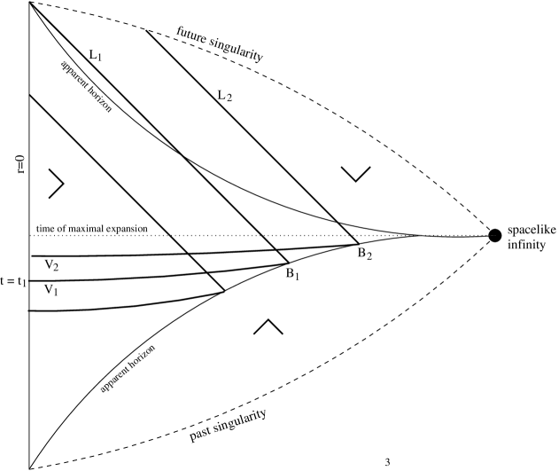
Figure 5: Penrose diagram for a flat universe with matter and a negative cosmological constant. Two apparent horizons divide the space-time into an anti-trapped, a trapped, and a normal region. The wedges show the light-sheet directions. The future-directed ingoing light-sheet $L_{1}$ of the surface $B_{1}$ is complete. By the spacelike projection theorem (Sec. 3.4), the entropy on the spatial region $V_{1}$ is bounded by the area of $B_{1}$. An apparent horizon surface $B_{2}$ at a later time, however, does not possess a complete future-directed ingoing light-sheet: $L_{2}$ is truncated by the future singularity. Therefore the area of $B_{2}$ bounds only the entropy on its three light-sheets, not on its spatial interior $V_{2}$.

shows, the universe starts out much like an ordinary flat FRW universe. As the normal matter is diluted, it eventually becomes dominated by the negative cosmological constant. This slows down the expansion of the universe so much that it starts to recollapse. The evolution is symmetric about the turn-around time. Eventually, matter dominates again and the universe ends in a big crunch. As the turnaround time is approached, the apparent horizon moves out to spatial infinity [15], and the enclosed volume grows without bound. The entropy density is constant, and the area grows more slowly than the volume. Thus the entropy eventually exceeds the Bak-Rey bound.

But the cosmological corollary (Sec. 5.1) states that one can use the interior of the apparent horizon for an entropy/area bound only if the future-directed ingoing light-sheet is complete. As Fig. 5 shows, this ceases to be the case before the turnaround time. After the time $t_{1}$, where $t_{1}<t_{\rm turnaround}$, the future-directed light-sheet of the apparent horizon will have another boundary, namely on the future singularity of the space-time. Thus the conditions for the spacelike projection theorem, and the corollary it implies, are no longer met. The entropy in the spatial interior of the apparent horizon [14] will not be bounded by its area in this region.

The covariant entropy conjecture states that the entropy on the future-directed ingoing light-sheet, as well as the two past-directed light-sheets of the apparent horizon will each be less than $A/4$. Because the future-directed light-sheet is truncated by the future singularity, and the past-directed light-sheets are truncated by the past singularity, the comoving volume swept out by any of these light-sheet grows only like the area as one moves further along the apparent horizon. Thus there is no contradiction with the covariant bound.

Neither is there any contradiction with the calculation performed in Sec. 4.2, which concluded that Bekenstein’s bound can be applied to the region within the apparent horizon. This calculation was done within the framework of Bekenstein’s conditions, and thus explicitly assumed the positivity of energy, which is violated here. As we pointed out in Sec. 1.1, Bekenstein’s bound cannot be applied to regions containing a negative energy component, such as a negative cosmological constant. This indicates a striking difference to the covariant bound. While we have formally assumed the positivity of energy as a condition for the covariant entropy bound, we have argued in Sec. 2 that the validity of the bound may well extend to space-times with a negative cosmological constant. We find ourselves encouraged by this example.

6 Testing the conjecture in gravitational collapse

In Sec. 4 we tested the covariant entropy conjecture for anti-trapped and normal surfaces in cosmological space-times. We found that even the most non-adiabatic processes can only saturate, but not violate, the bound. We now turn to trapped surfaces, which occur not only in collapsing universes, but arise generally during gravitational collapse and inside black holes.

Like anti-trapped regions, trapped regions are manifestly dominated by self-gravity, and Bekenstein’s bound will be of little help. The covariant entropy bound must be justified by other considerations. This is a more subtle problem for trapped, than for anti-trapped surfaces. It was reasonable to require (Sec. 4.1) that the entropy one Planck time away from a past singularity cannot exceed one per Planck volume; this merely amounts to a sensible specification of initial conditions. Because of the rapid expansion, the entropy/area ratio decreases at later times, and a situation in which the covariant bound would be exceeded does not arise. But near future singularities, one cannot use the time-reverse of this argument to “retrodict” that some experimental setup was impossible to start with. Initial conditions are set in the past, not in the future.

At first sight it seems obvious that the covariant entropy bound, like any entropy/area bound, will be violated in trapped regions. Consider a saturated Bekenstein system of area $A_{0}$, in which gravitational collapse is induced. The system will shrink, but by the second law, the entropy will not decrease. A short time after the beginning of the collapse, the surface of the system will have an area $A_{1}<A_{0}$. Because the surface is trapped, the past-directed ingoing light-rays have positive expansion and cannot be considered. But there will be a future-directed ingoing light-sheet. If this light-sheet penetrated the entire system, it would contain an entropy of $S\geq A_{0}/4>A_{1}/4$ and the bound would be exceeded. There are a number of effects, however, which constrain the extent to which the light-sheet can sample entropy. We will discuss them qualitatively, before turning to a quantitative test in Sec. 6.2.

6.1 Light-sheet penetration into collapsing systems

When the boundary of the system is a suffiently small proper time away from the future singularity, the light-sheet will not intersect the whole system, because it will be truncated by the singularity (or a surface where the Planck density is reached), much like the past light-sheet of spheres larger than the particle horizon in a flat FRW universe. Truncation is a basic limitation [12], but additional constraints will be needed.

Consider the Oppenheimer-Snyder collapse of a dust ball [20], commencing from a momentarily static state with $R=2M$, as shown in Fig. 6.

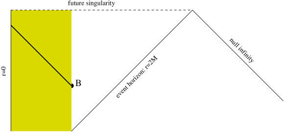
Figure 6: Penrose diagram for the Oppenheimer-Snyder collapse of a dust star. The interior of the star is described by a portion of the closed dust-dominated FRW solution. Correspondingly, it is represented by the top left quarter of the Penrose diagram, Fig. 4. The exterior is a portion of the Schwarzschild solution. Light-rays emitted from the surface of the star when it is inside its gravitational radius can traverse the interior entirely. This is not a violation of the covariant entropy bound because a collapsing dust star does not have much entropy. For highly enthopic collapsing objects, a number of effects must be taken into account which protect the conjecture (see text).

A future-directed ingoing light-sheet, starting at the surface $B$ at a sufficiently early time but inside the event horizon, can easily traverse the ball before the singularity (or the Planck density, at $R\sim M^{1/3}$) is reached. But this light-sheet would endanger the bound only if the system collapsed from a state in which it nearly saturated Bekenstein’s bound. So how much entropy does the dust star actually contain? Strictly, the Oppenheimer-Snyder solution describes a dust ball at zero temperature. Since it also must be exactly homogeneous, it contains not even the usual positional entropy equal to the particle number. Thus the entropy is zero. In order to introduce a sizable amount of entropy, we have to violate the conditions under which the solution is valid: homogeneity and zero temperature. This collapse will be described by a different solution, for which a detailed calculation would have to be done to determine the penetration depth of light-sheets.

By definition, highly enthropic systems undergoing gravitational collapse are very irregular internally and contain strong small scale density perturbations. This will make the collapse inhomogeneous, with some regions reaching the singularity after a shorter proper time than other regions. One might call this effect Local Gravitational Collapse. A saturated Bekenstein system is globally just on the verge of gravitational collapse: $R=2M$. But as it contracts, individual parts of the system, of size $\Delta R<R$ will become gravitationally unstable: $\Delta R\leq 2\Delta M$. Particles in an overdense region will reach a singularity after a proper time of order $\Delta R^{2}/\Delta M$, which is shorter than the remaining lifetime of average regions, $\sim R^{2}/M$. This makes it more difficult for a light-sheet to penetrate the system completely, unless it originates near the beginning of the collapse, when the area is still large.

The internal irregularity of highly enthropic systems also enhances the effect of Percolation, discussed in Sec. 3.3. Inhomogeneities that break spherical symmetry will deflect the rays in the light-sheet and cause dents in their spherical cross-sections. Such dents will develop into “angular” caustics. At any caustic, the light-sheet ends, because the expansion becomes positive (Sec. 3.2). Any light-rays that do not end on caustics will follow an irregular path through the object similar to random walk. Since they waste affine time on covering angular directions, they may not proceed far into the object before the singularity is reached. Thus it may well be impossible for a light-sheet to penetrate through a collapsing, highly entropic system far enough to sample excessive entropy.

The quantitative investigation of the formation of angular caustics on light-sheets penetrating collapsing, highly enthropic systems lies beyond the scope of this paper. A strong, quantitative case for the validity of the bound may still be made by eliminating the percolation effect. We will consider a system containing only radial modes. This system is spherically symmetric even microscopically, and cannot deflect light-rays into angular directions. With no constraints on mass and size, it can contain arbitrary amounts of entropy, but cannot lead to angular caustics on the light-sheet.

6.2 A quantitative test

Consider a Schwarzschild black hole of horizon size $r_{0}$ (see Fig. 7).

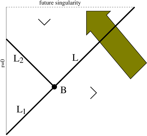
Figure 7: Penrose diagram for a black hole. $B$ is a surface on the apparent horizon and has three light-sheets: $L_{1}$, $L_{2}$, and $L$. In an attempt to violate the covariant entropy conjecture, we collapse a massive shell around the black hole. We find, however, that one cannot squeeze more entropy through $L$ than a quarter of the area of $B$. Otherwise, $L$ reaches the singularity before passing through the infalling shell entirely.

Let $B$ be a sphere on the apparent horizon at some given time; thus $B$ has area

$$A=4\pi r_{0}^{2}.$$ (6.1)

The surface $B$ is marginally outer trapped and possesses three light-sheets. The past-directed ingoing light-sheet, $L_{1}$ counts the entropy $S_{\rm in}$ that went into the black hole. The generalized second law of thermodynamics guarantees that the entropy conjecture will hold on this light-sheet, since

$$A/4=S_{\rm bh}\geq S_{\rm in}.$$ (6.2)

The future-directed ingoing light-sheet, $L_{2}$, may intersect some or all of the collapsing object that formed the black hole. The future-directed outgoing light-sheet $L$ intersects objects falling into the black hole at a later time. The validity of the conjecture for the future-directed light-sheets was supported by qualitative arguments in the previous subsection. For a quantitative test, we shall now try to send excessive entropy through $L$.

$L$ has zero expansion and defines the black hole horizon as long as no additional matter falls in. When $L$ does encounter matter, the expansion becomes negative and $L$ collapses to $r=0$ within a finite affine time. Our strategy will be to use an infalling shell of matter to squeeze as much entropy as possible across $L$ before the light-sheet ends on a caustic or a singularity. We shall not have any scruples about making the mass of the shell extremely large compared to the mass of the black hole. By preparing the shell far outside the black hole and letting it collapse, we can thus transport an arbitrary amount of entropy to $r_{0}$. This means, of course, that the shell may be well inside its own Schwarzschild radius by the time it reaches $L$; but by the second law, this cannot reduce the entropy it carries. What we must ensure, however, is that $L$ actually penetrates the entire shell and samples all of its entropy. We will now show that this requirement keeps the shell entropy within the conjectured bound.

Let $\theta$ be the expansion of the null generators of $L$. Its rate of change is given by Raychauduri’s equation, Eq. (3.2), from which we obtain the inequality

$$\frac{d\theta}{d\lambda}\leq-\frac{1}{2}\theta^{2}-8\pi T_{ab}k^{a}k^{b}.$$ (6.3)

The first term on the right hand side is non-positive, and the dominant energy condition is sufficient to ensure that the second term is also non-positive. Initially, $\theta=0$, since $L$ is an apparent horizon. Now consider a shell of matter, of mass $M$, crossing the light-sheet $L$. We would like to make the shell as wide as possible in order to store a lot of entropy. But we also must keep it sufficiently thin, so that the light-sheet does not collapse due to the first term in Eq. (6.3), before the shell has completely crossed it.

The maximum width of the shell can be easily estimated. Consider an infinitely thin shell of mass $M$ falling towards the black hole at $r_{0}$. Outside the shell, the metric will be given by a Schwarzschild black hole of mass

$$\tilde{M}=M+\frac{r_{0}}{2},$$ (6.4)

by Birkhoff’s theorem. Once the shell has crossed the light-sheet $L$ at $r_{0}$, the null generators of $L$ will be moving in a Schwarzschild interior of mass $\tilde{M}$. Therefore this meeting occurs at proper time

$$\Delta\tau_{\rm dead}=r_{0}+2\tilde{M}\ln\left(1-\frac{r_{0}}{2\tilde{M}}\right)\approx\frac{r_{0}^{2}}{4\tilde{M}}$$ (6.5)

before the generators reach a singularity. We may approximate a shell of finite proper thickness $w$ by an infinitely thin shell of the same mass, located $w/2$ from either side. We are thus pretending that the shell mass contributes to the second term of the Raychauduri equation all at once, at the moment when half of the shell has already passed through $L$. Since we require that the light-sheet penetrates the shell entirely, we must be sure that the other half of the shell passes through $L$ before the light-sheet hits the singularity. This requires $w/2\leq\Delta\tau_{\rm dead}$, whence

$$w_{\rm max}\approx r_{0}^{2}/2\tilde{M}.$$ (6.6)

The maximum width of the shell is thus inversely proportional to its mass, and is always less than $r_{0}$.

The next step will be to calculate the maximum entropy of a spherical shell of mass $M$ and width $w$. We will build the shell at $r=R$, far away from the black hole and outside its own gravitational radius; i.e., $R$ is much greater than any of the quantities $w$, $M$, and $r_{0}$. Thus Bekenstein’s bound can be used to estimate the entropy. Then we will let the shell collapse into the black hole. Since $w_{\rm max}<r_{0}/2$ by Eq. (6.6), the width of the shell will be smaller than the curvature of space during the entire time of the collapse, and we can take it to remain constant. This enables us to neglect effects of local gravitational collapse (which, if included, constrain the setup further; see Sec. 6.1). In order to exclude effects of angular caustics, which are difficult to deal with quantitatively, we must specify that the shell contain only spherically symmetric micro-states, i.e., micro-states living in the radial, not the angular directions. We will now estimate the maximum entropy of the shell.

The shell can be split into a large number $n=R^{2}/w^{2}$ of roughly cubic boxes of volume $w^{3}$ and mass $M/n$, separated by impenetrable radial walls. By Eq. (1.1), the maximum entropy of an isolated, single box is the largest dimension times the mass:

$$S_{\rm box}=2\pi w\frac{M}{n}.$$ (6.7)

Since all states are restricted to be radial, no new states are added by removing the wall between two adjacent boxes. Thus the entropy of two boxes will simply be twice the entropy of one box. By repeating this argument, we can remove all the separating walls. Therefore the shell has a maximum entropy of

$$S_{\rm shell}=2\pi wM.$$ (6.8)

The width $w$ is restricted by Eq. (6.6). One has $M/\tilde{M}\leq 1$ by Eq. (6.4), even if the limit $M\rightarrow\infty$ is permitted. Thus the shell entropy cannot exceed $\pi r_{0}^{2}$, which by Eq. (6.1) is a quarter of the area bounding the light-sheet:

$$S_{\rm shell}\leq\frac{A}{4}.$$ (6.9)

We conclude that $A/4$ is the maximum amount of entropy one can transport through a future-directed outgoing light-sheet $L$ bounded by a black hole apparent horizon of area $A$, using an exactly spherically symmetric shell of matter. We take this as strong evidence in favor of the entropy bound we propose.

7 Conclusions

Bekenstein has shown that the entropy of a thermodynamic system with limited self-gravity is bounded by its area. By demanding general coordinate invariance and constructing a selection rule, we arrived at a bound on the entropy present on null hypersurfaces in arbitrary space-times. We tested the conjecture on cosmological solutions and inside gravitationally collapsing regions. We found, under the most adverse assumptions, that the bound can be saturated but not exceeded. This evidence suggests that the covariant entropy conjecture may be a universal law of physics.

But can the conjecture be proven? The processes by which the bound is protected appear to be rather subtle. They differ according to the physical situation studied, and they can involve combinations of different effects more reminiscent of a conspiracy than of an elegant mechanism (Sec. 6.1). (This is quite in contrast to Bekenstein’s bound, which is protected by gravitational collapse; see below.) We have verified the bound in a wide class of space-times and space-time regions, but from the perspective of general relativity, the processes protecting the bound appear eclectic, and its success remains mysterious. This indicates that we may be looking at nature in an artificial and complicated way when we describe it as a $3+1$-dimensional space-time filled with matter. If the covariant bound is correct, we believe it must arise from a more fundamental description of nature in an obvious way. But this does not exclude the possibility that it can be proven (in a complicated way) entirely within general relativity. The proof would have to combine the tools used for establishing the laws of black hole mechanics [22] with the formalism of the Hawking-Penrose singularity theorems [18].

In the final paragraphs of Secs. 3.1 and 3.4 we discussed the most important property of the conjecture: It is manifestly time reversal invariant. Therefore the second law of thermodynamics, which underlies Bekenstein’s bound, cannot be responsible for the covariant bound, and one is forced to contemplate the possibility of a different origin.

As a thermodynamic concept, entropy has a built-in arrow of time. The T-invariance of the covariant entropy conjecture can be understood only if the bound is interpreted as a bound on the number of degrees of freedom of the matter systems present on the light-sheets. This number is always at least as large as the thermodynamic entropy. With this statistical interpretation, T-invariance is natural. However, we never made any assumptions about the microscopic properties of matter, which would limit the number of degrees of freedom present. This leaves no choice but to conclude that the number of degrees of freedom in nature is fundamentally limited, as proposed in Refs. [10, 11].

The idea that the world is effectively two-dimensional was put forth by ’t Hooft [10] and was further developed by Susskind [11]. Based on Bekenstein’s bound, the holographic hypothesis was a bold leap. One could argue, after all, that Bekenstein’s bound is not a fundamental limit on the number of degrees of freedom, but a practical restriction on thermodynamic entropy. There could be far more degrees of freedom in a system than its surface area, but if too many of them were excited at the same time, a black hole would form and the system would no longer satisfy Bekenstein’s conditions. One may view Bekenstein’s bound as arising from this elegant gravitational collapse mechanism. Bekenstein’s law applies only to Bekenstein systems; it works because a Bekenstein system exceeding the bound ceases to be one.

The covariant entropy bound, on the other hand, applies even to surfaces in collapsing regions, or on cosmological scales. Its generality, together with its T-invariance, force us to the conclusion that a holographic principle underlies the description of nature. Moreover, the bound leads naturally to a background-independent formulation of the principle. The number of independent degrees of freedom on any light-sheet of a surface $B$ cannot exceed a quarter of the area of $B$.

References

- [1] J. D. Bekenstein: A universal upper bound on the entropy to energy ratio for bounded systems. Phys. Rev. D 23, 287 (1981).
- [2] J. D. Bekenstein: Black holes and the second law. Nuovo Cim. Lett. 4, 737 (1972).
- [3] J. D. Bekenstein: Black holes and entropy. Phys. Rev. D 7, 2333 (1973).
- [4] J. D. Bekenstein: Generalized second law of thermodynamics in black hole physics. Phys. Rev. D 9, 3292 (1974).
- [5] S. W. Hawking: Particle creation by black holes. Commun. Math. Phys. 43, 199 (1974).
- [6] J. D. Bekenstein: Do we understand black hole entropy? gr-qc/9409015.
- [7] D. N. Page: Particle emission rates from a black hole. II. Massless particles from a rotating hole. Phys. Rev. D 14, 3260 (1976).
- [8] M. Schiffer and J. D. Bekenstein: Proof of the quantum bound on specific entropy for free fields. Phys. Rev. D 39, 1109 (1989).
- [9] W. Fischler and L. Susskind: Holography and cosmology, hep-th/9806039.
- [10] G. ’t Hooft: Dimensional reduction in quantum gravity, gr-qc/9310026.
- [11] L. Susskind: The world as a hologram. J. Math. Phys. 36, 6377 (1995), hep-th/9409089.
- [12] R. Easther and D. A. Lowe: Holography, cosmology and the second law of thermodynamics, hep-th/9902088.
- [13] G. Veneziano: Pre-bangian origin of our entropy and time arrow, hep-th/9902126.
- [14] D. Bak and S.-J. Rey: Cosmic holography, hep-th/9902173.
- [15] N. Kaloper and A. Linde: Cosmology vs. holography, hep-th/9904120.
- [16] R. Brustein: The generalized second law of thermodynamics in cosmology, gr-qc/9904061.
- [17] S. Corley and T. Jacobson: Focusing and the holographic hypothesis. Phys. Rev. D 53, 6720 (1996), gr-qc/9602043.
- [18] S. W. Hawking and G. F. R. Ellis: The large scale stucture of space-time. Cambridge University Press, Cambridge, England (1973).
- [19] R. M. Wald: General Relativity. The University of Chicago Press, Chicago (1984).
- [20] C. W. Misner, K. S. Thorne and J. A. Wheeler (eds.): Gravitation. Freeman, New York (1973).
- [21] J. D. Bekenstein: Is the cosmological singularity thermodynamically possible? Int. J. Theor. Phys. 28, 967 (1989).
- [22] J. M. Bardeen, B. Carter and S. W. Hawking: The four laws of black hole mechanics. Commun. Math. Phys. 31, 161 (1973).