The holographic principle

Abstract

There is strong evidence that the area of any surface limits the information content of adjacent spacetime regions, at $1.4\times 10^{69}$ bits per square meter. We review the developments that have led to the recognition of this entropy bound, placing special emphasis on the quantum properties of black holes. The construction of light-sheets, which associate relevant spacetime regions to any given surface, is discussed in detail. We explain how the bound is tested and demonstrate its validity in a wide range of examples.

A universal relation between geometry and information is thus uncovered. It has yet to be explained. The holographic principle asserts that its origin must lie in the number of fundamental degrees of freedom involved in a unified description of spacetime and matter. It must be manifest in an underlying quantum theory of gravity. We survey some successes and challenges in implementing the holographic principle.

I Introduction

I.1 A principle for quantum gravity

Progress in fundamental physics has often been driven by the recognition of a new principle, a key insight to guide the search for a successful theory. Examples include the principles of relativity, the equivalence principle, and the gauge principle. Such principles lay down general properties that must be incorporated into the laws of physics.

A principle can be sparked by contradictions between existing theories. By judiciously declaring which theory contains the elements of a unified framework, a principle may force other theories to be adapted or superceded. The special theory of relativity, for example, reconciles electrodynamics with Galilean kinematics at the expense of the latter.

A principle can also arise from some newly recognized pattern, an apparent law of physics that stands by itself, both uncontradicted and unexplained by existing theories. A principle may declare this pattern to be at the core of a new theory altogether.

In Newtonian gravity, for example, the proportionality of gravitational and inertial mass in all bodies seems a curious coincidence that is far from inevitable. The equivalence principle demands that this pattern must be made manifest in a new theory. This led Einstein to the general theory of relativity, in which the equality of gravitational and inertial mass is built in from the start. Because all bodies follow geodesics in a curved spacetime, things simply couldn’t be otherwise.

The holographic principle belongs in the latter class. The unexplained “pattern”, in this case, is the existence of a precise, general, and surprisingly strong limit on the information content of spacetime regions. This pattern has come to be recognized in stages; its present, most general form is called the covariant entropy bound. The holographic principle asserts that this bound is not a coincidence, but that its origin must be found in a new theory.

The covariant entropy bound relates aspects of spacetime geometry to the number of quantum states of matter. This suggests that any theory that incorporates the holographic principle must unify matter, gravity, and quantum mechanics. It will be a quantum theory of gravity, a framework that transcends general relativity and quantum field theory.

This expectation is supported by the close ties between the covariant entropy bound and the semi-classical properties of black holes. It has been confirmed—albeit in a limited context—by recent results in string theory.

The holographic principle conflicts with received wisdom; in this sense, it also belongs in the former class. Conventional theories are local; quantum field theory, for example, contains degrees of freedom at every point in space. Even with a short distance cutoff, the information content of a spatial region would appear to grow with the volume. The holographic principle, on the other hand, implies that the number of fundamental degrees of freedom is related to the area of surfaces in spacetime. Typically, this number is drastically smaller than the field theory estimate.

Thus, the holographic principle calls into question not only the fundamental status of field theory but the very notion of locality. It gives preference, as we shall see, to the preservation of quantum-mechanical unitarity.

In physics, information can be encoded in a variety of ways: by the quantum states, say, of a conformal field theory, or by a lattice of spins. Unfortunately, for all its precise predictions about the number of fundamental degrees of freedom in spacetime, the holographic principle betrays little about their character. The amount of information is strictly determined, but not its form. It is interesting to contemplate the notion that pure, abstract information may underlie all of physics. But for now, this austerity frustrates the design of concrete models incorporating the holographic principle.

Indeed, a broader caveat is called for. The covariant entropy bound is a compelling pattern, but it may still prove incorrect or merely accidental, signifying no deeper origin. If the bound does stem from a fundamental theory, that relation could be indirect or peripheral, in which case the holographic principle would be unlikely to guide us to the core ideas of the theory. All that aside, the holographic principle is likely only one of several independent conceptual advances needed for progress in quantum gravity.

At present, however, quantum gravity poses an immense problem tackled with little guidance. Quantum gravity has imprinted few traces on physics below the Planck energy. Among them, the information content of spacetime may well be the most profound.

The direction offered by the holographic principle is impacting existing frameworks and provoking new approaches. In particular, it may prove beneficial to the further development of string theory, widely (and, in our view, justly) considered the most compelling of present approaches.

This article will outline the case for the holographic principle whilst providing a starting point for further study of the literature. The material is not, for the most part, technical. The main mathematical aspect, the construction of light-sheets, is rather straightforward. In order to achieve a self-contained presentation, some basic material on general relativity has been included in an appendix.

In demonstrating the scope and power of the holographic correspondence between areas and information, our ultimate task is to convey its character as a law of physics that captures one of the most intriguing aspects of quantum gravity. If the reader is led to contemplate the origin of this particular pattern nature has laid out, our review will have succeeded.

I.2 Notation and conventions

Throughout this paper, Planck units will be used:

$$\hbar=G=c=k=1,$$ (1)

where $G$ is Newton’s constant, $\hbar$ is Planck’s constant, $c$ is the speed of light, and $k$ is Boltzmann’s constant. In particular, all areas are measured in multiples of the square of the Planck length,

$$l_{\rm P}^{2}={G\hbar\over c^{3}}=2.59\times 10^{-66}\mbox{cm}^{2}.$$ (2)

The Planck units of energy density, mass, temperature, and other quantities are converted to cgs units, e.g., in Wald (1984), whose conventions we follow in general. For a small number of key formulas, we will provide an alternate expression in which all constants are given explicitly.

We consider spacetimes of arbitrary dimension $D\geq 4$, unless noted otherwise. In explicit examples we often take $D=4$ for definiteness. The appendix fixes the metric signature and defines “surface”, “hypersurface”, “null”, and many other terms from general relativity. The term “light-sheet” is defined in Sec. V.

“GSL” stands for the generalized second law of thermodynamics (Sec. II.1.3). The number of degrees of freedom of a quantum system, $N$, is defined as the logarithm of the dimension, ${\cal N}$, of its Hilbert space in Sec. III.1. Equivalently, $N$ can be defined as the number of bits of information times $\ln 2$.

I.3 Outline

In Sec. II, we review Bekenstein’s (1972) notion of black hole entropy and the related discovery of upper bounds on the entropy of matter systems. Assuming weak gravity, spherical symmetry, and other conditions, one finds that the entropy in a region of space is limited by the area of its boundary. Based on this “spherical entropy bound”, ’t Hooft (1993) and Susskind (1995b) formulated a holographic principle. We discuss motivations for this radical step.

The spherical entropy bound depends on assumptions that are clearly violated by realistic physical systems. A priori there is no reason to expect that the bound has universal validity, nor that it admits a reformulation that does. Yet, if the number of degrees of freedom in nature is as small as ’t Hooft and Susskind asserted, one would expect wider implications for the maximal entropy of matter.

In Sec. IV, however, we demonstrate that a naive generalization of the spherical entropy bound is unsuccessful. The “spacelike entropy bound” states that the entropy in a given spatial volume, irrespective of shape and location, is always less than the surface area of its boundary. We consider four examples of realistic, commonplace physical systems, and find that the spacelike entropy bound is violated in each one of them.

In light of these difficulties, some authors, forgoing complete generality, searched instead for reliable conditions under which the spacelike entropy bound holds. We review the difficulties faced in making such conditions precise even in simple cosmological models.

Thus, the idea that the area of surfaces generally bounds the entropy in enclosed spatial volumes has proven wrong; it can be neither the basis nor the consequence of a fundamental principle. This review would be incomplete if it failed to stress this point. Moreover, the ease with which the spacelike entropy bound (and several of its modifications) can be excluded underscores that a general entropy bound, if found, is no triviality. The counterexamples to the spacelike bound later provide a useful testing ground for the covariant bound.

Inadequacies of the spacelike entropy bound led Fischler and Susskind (1998) to a bound involving light cones. The covariant entropy bound (Bousso, 1999a), presented in Sec. V, refines and generalizes this approach. Given any surface $B$, the bound states that the entropy on any light-sheet of $B$ will not exceed the area of $B$. Light-sheets are particular hypersurfaces generated by light rays orthogonal to $B$. The light rays may only be followed as long as they are not expanding. We explain this construction in detail.

After discussing how to define the entropy on a light-sheet, we spell out known limitations of the covariant entropy bound. The bound is presently formulated only for approximately classical geometries, and one must exclude unphysical matter content, such as large negative energy. We conclude that the covariant entropy bound is well-defined and testable in a vast class of solutions. This includes all thermodynamic systems and cosmologies presently known or considered realistic.

In Sec. VI we review the geometric properties of light-sheets, which are central to the operation of the covariant entropy bound. Raychaudhuri’s equation is used to analyse the effects of entropy on light-sheet evolution. By construction, a light-sheet is generated by light rays that are initially either parallel or contracting. Entropic matter systems carry mass, which causes the bending of light.

This means that the light rays generating a light-sheet will be focussed towards each other when they encounter entropy. Eventually they self-intersect in a caustic, where they must be terminated because they would begin to expand. This mechanism would provide an “explanation” of the covariant entropy bound if one could show that the mass associated with entropy is necessarily so large that light-sheets focus and terminate before they encounter more entropy than their initial area.

Unfortunately, present theories do not impose an independent, fundamental lower bound on the energetic price of entropy. However, Flanagan, Marolf, and Wald (2000) were able to identify conditions on entropy density which are widely satisfied in nature and which are sufficient to guarantee the validity of the covariant entropy bound. We review these conditions.

The covariant bound can also be used to obtain sufficient criteria under which the spacelike entropy bound holds. Roughly, these criteria can be summarized by demanding that gravity be weak. However, the precise condition requires the construction of light-sheets; it cannot be formulated in terms of intrinsic properties of spatial volumes.

The event horizon of a black hole is a light-sheet of its final surface area. Thus, the covariant entropy bound includes to the generalized second law of thermodynamics in black hole formation as a special case. More broadly, the generalized second law, as well as the Bekenstein entropy bound, follow from a strengthened version of the covariant entropy bound.

In Sec. VII, the covariant entropy bound is applied to a variety of thermodynamic systems and cosmological spacetimes. This includes all of the examples in which the spacelike entropy bound is violated. We find that the covariant bound is satisfied in each case.

In particular, the bound is found to hold in strongly gravitating regions, such as cosmological spacetimes and collapsing objects. Aside from providing evidence for the general validity of the bound, this demonstrates that the bound (unlike the spherical entropy bound) holds in a regime where it cannot be derived from black hole thermodynamics.

In Sec. VIII, we arrive at the holographic principle. We note that the covariant entropy bound holds with remarkable generality but is not logically implied by known laws of physics. We conclude that the bound has a fundamental origin. As a universal limitation on the information content of Lorentzian geometry, the bound should be manifest in a quantum theory of gravity. We formulate the holographic principle and list some of its implications. The principle poses a challenge for local theories. It suggests a preferred role for null hypersurfaces in the classical limit of quantum gravity.

In Sec. IX we analyze an example of a holographic theory. Quantum gravity in certain asymptotically Anti-de Sitter spacetimes is fully defined by a conformal field theory. The latter theory contains the correct number of degrees of freedom demanded by the holographic principle. It can be thought of as living on a kind of holographic screen at the boundary of spacetime and containing one bit of information per Planck area.

Holographic screens with this information density can be constructed for arbitrary spacetimes—in this sense, the world is a hologram. In most other respects, however, global holographic screens do not generally support the notion that a holographic theory is a conventional field theory living at the boundary of a spacetime.

At present, there is much interest in finding more general holographic theories. We discuss the extent to which string theory, and a number of other approaches, have realized this goal. A particular area of focus is de Sitter space, which exhibits an absolute entropy bound. We review the implications of the holographic principle in such spacetimes.

I.4 Related subjects and further reading

The holographic principle has developed from a large set of ideas and results, not all of which seemed mutually related at first. This is not a historical review; we have aimed mainly at achieving a coherent, modern perspective on the holographic principle. We do not give equal emphasis to all developments, and we respect the historical order only where it serves the clarity of exposition. Along with length constraints, however, this approach has led to some omissions and shortcomings, for which we apologize.

We have chosen to focus on the covariant entropy bound because it can be tested using only quantum field theory and general relativity. Its universality motivates the holographic principle independently of any particular ansatz for quantum gravity (say, string theory) and without additional assumptions (such as unitarity). It yields a precise and general formulation.

Historically, the idea of the holographic principle was tied, in part, to the debate about information loss in black holes and to the notion of black hole complementarity. Although we identify some of the connections, our treatment of these issues is far from comprehensive. Reviews include Thorlacius (1995), Verlinde (1995), Susskind and Uglum (1996), Bigatti and Susskind (2000), and Wald (2001).

Some aspects of what we now recognize as the holographic principle were encountered, at an early stage, as features of string theory. (This is as it should be, since string theory is a quantum theory of gravity.) In the infinite momentum frame, the theory admits a lower-dimensional description from which the gravitational dynamics of the full spacetime arises non-trivially (Giles and Thorn, 1977; Giles, McLerran, and Thorn, 1978; Thorn, 1979, 1991, 1995, 1996; Klebanov and Susskind, 1988). Susskind (1995b) placed this property of string theory in the context of the holographic principle and related it to black hole thermodynamics and entropy limitations.

Some authors have traced the emergence of the holographic principle also to other approaches to quantum gravity; see Smolin (2001) for a discussion and further references.

By tracing over a region of space one obtains a density matrix. Bombelli et al. (1986) showed that the resulting entropy is proportional to the boundary area of the region. A more general argument was given by Srednicki (1993). Gravity does not enter in this consideration. Moreover, the entanglement entropy is generally unrelated to the size of the Hilbert space describing either side of the boundary. Thus, it is not clear to what extent this suggestive result is related to the holographic principle.

This is not a review of the AdS/CFT correspondence (Maldacena, 1998; see also Gubser, Klebanov, and Polyakov, 1998; Witten, 1998). This rich and beautiful duality can be regarded (among its many interesting aspects) as an implementation of the holographic principle in a concrete model. Unfortunately, it applies only to a narrow class of spacetimes of limited physical relevance. By contrast, the holographic principle claims a far greater level of generality—a level at which it continues to lack a concrete implementation.

We will broadly discuss the relation between the AdS/CFT correspondence and the holographic principle, but we will not dwell on aspects that seem particular to AdS/CFT. (In particular, this means that the reader should not expect a discussion of every paper containing the word “holographic” in the title!) A detailed treatment of AdS/CFT would go beyond the purpose of the present text. An extensive review has been given by Aharony et al. (2000).

The AdS/CFT correspondence is closely related to some recent models of our 3+1 dimensional world as a defect, or brane, in a 4+1 dimensional AdS space. In the models of Randall and Sundrum (1999a,b), the gravitational degrees of freedom of the extra dimension appear on the brane as a dual field theory under the AdS/CFT correspondence. While the holographic principle can be considered a prerequisite for the existence of such models, their detailed discussion would not significantly strengthen our discourse. Earlier seminal papers in this area include Hořava and Witten (1996a,b).

A number of authors (e.g., Brustein and Veneziano, 2000; Verlinde, 2000; Brustein, Foffa, and Veneziano, 2001; see Cai, Myung, and Ohta, 2001, for additional references) have discussed interesting bounds which are not directly based on the area of surfaces. Not all of these bounds appear to be universal. Because their relation to the holographic principle is not entirely clear, we will not attempt to discuss them here. Applications of entropy bounds to string cosmology (e.g., Veneziano, 1999a; Bak and Rey, 2000b; Brustein, Foffa, and Sturani, 2000) are reviewed by Veneziano (2000).

The holographic principle has sometimes been said to exclude certain physically acceptable solutions of Einstein’s equations because they appeared to conflict with an entropy bound. The covariant bound has exposed these tensions as artifacts of the limitations of earlier entropy bounds. Indeed, this review bases the case for a holographic principle to a large part on the very generality of the covariant bound. However, the holographic principle does limit the applicability of quantum field theory on cosmologically large scales. It calls into question the conventional analysis of the cosmological constant problem (Cohen, Kaplan, and Nelson, 1999; Hořava, 1999; Banks, 2000a; Hořava and Minic, 2000; Thomas, 2000). It has also been applied to the calculation of anisotropies in the cosmic microwave background (Hogan, 2002a,b). The study of cosmological signatures of the holographic principle may be of great value, since it is not clear whether more conventional imprints of short-distance physics on the early universe are observable even in principle (see, e.g., Kaloper et al., 2002, and references therein).

Most attempts at implementing the holographic principle in a unified theory are still in their infancy. It would be premature to attempt a detailed review; some references are given in Sec. IX.4.

Other recent reviews overlapping with some or all of the topics covered here are Bigatti and Susskind (2000), Bousso (2000a), ’t Hooft (2000b), Bekenstein (2001) and Wald (2001). Relevant textbooks include Hawking and Ellis (1973); Misner, Thorne, and Wheeler (1973); Wald (1984, 1994); Green, Schwarz, and Witten (1987); and Polchinski (1998).

II Entropy bounds from black holes

This section reviews black hole entropy, some of the entropy bounds that have been inferred from it, and their relation to ’t Hooft’s (1993) and Susskind’s (1995b) proposal of a holographic principle.

The entropy bounds discussed in this section are “universal” (Bekenstein, 1981) in the sense that they are independent of the specific characteristics and composition of matter systems. Their validity is not truly universal, however, because they apply only when gravity is weak.

We consider only Einstein gravity. For black hole thermodynamics in higher-derivative gravity, see, e.g., Myers and Simon (1988), Jacobson and Myers (1993), Wald (1993), Iyer and Wald (1994, 1995), Jacobson, Kang, and Myers (1994), and the review by Myers (1998).

II.1 Black hole thermodynamics

The notion of black hole entropy is motivated by two results in general relativity.

II.1.1 Area theorem

The area theorem (Hawking, 1971) states that the area of a black hole event horizon never decreases with time:

$$dA\geq 0.$$ (3)

Moreover, if two black holes merge, the area of the new black hole will exceed the total area of the original black holes.

For example, an object falling into a Schwarzschild black hole will increase the mass of the black hole, $M$. Hence the horizon area, $A=16\pi M^{2}$ in $D=4$, increases. On the other hand, one would not expect the area to decrease in any classical process, because the black hole cannot emit particles.

The theorem suggests an analogy between black hole area and thermodynamic entropy.

II.1.2 No-hair theorem

Work of Israel (1967, 1968), Carter (1970), Hawking (1971, 1972), and others, implies the curiously named no-hair theorem: A stationary black hole is characterized by only three quantities: mass, angular momentum, and charge.

Consider a complex matter system, such as a star, that collapses to form a black hole. The black hole will eventually settle down into a final, stationary state. The no-hair theorem implies that this state is unique.

From an outside observer’s point of view, the formation of a black hole appears to violate the second law of thermodynamics. The phase space appears to be drastically reduced. The collapsing system may have arbitrarily large entropy, but the final state has none at all. Different initial conditions will lead to indistinguishable results.

A similar problem arises when a matter system is dropped into an existing black hole. Geroch has proposed a further method for violating the second law, which exploits a classical black hole to transform heat into work; see Bekenstein (1972) for details.

II.1.3 Bekenstein entropy and the generalized second law

Thus, the no-hair theorem poses a paradox, to which the area theorem suggests a resolution. When a thermodynamic system disappears behind a black hole’s event horizon, its entropy is lost to an outside observer. The area of the event horizon will typically grow when the black hole swallows the system. Perhaps one could regard this area increase as a kind of compensation for the loss of matter entropy?

Based on this reasoning, Bekenstein (1972, 1973, 1974) suggested that a black hole actually carries an entropy equal to its horizon area, $S_{\rm BH}=\eta A$, where $\eta$ is a number of order unity. In Sec. II.1.4 it will be seen that $\eta={1\over 4}$ (Hawking, 1974):

$$S_{\rm BH}={A\over 4}.$$ (4)

[In full, $S_{\rm BH}=kAc^{3}/(4G\hbar)$.] The entropy of a black hole is given by a quarter of the area of its horizon in Planck units. In ordinary units, it is the horizon area divided by about $10^{-69}$m².

Moreover, Bekenstein (1972, 1973, 1974) proposed that the second law of thermodynamics holds only for the sum of black hole entropy and matter entropy:

$$dS_{\rm total}\geq 0.$$ (5)

For ordinary matter systems alone, the second law need not hold. But if the entropy of black holes, Eq. (4), is included in the balance, the total entropy will never decrease. This is referred to as the generalized second law or GSL.

The content of this statement may be illustrated as follows. Consider a thermodynamic system ${\cal T}$, consisting of well-separated, non-interacting components. Some components, labeled ${\cal C}_{i}$, may be thermodynamic systems made from ordinary matter, with entropy $S({\cal C}_{i})$. The other components, ${\cal B}_{j}$, are black holes, with horizon areas $A_{j}$. The total entropy of ${\cal T}$ is given by

$$S_{\rm total}^{\rm initial}=S_{\rm matter}+S_{\rm BH}.$$ (6)

Here, $S_{\rm matter}=\sum S({\cal C}_{i})$ is the total entropy of all ordinary matter. $S_{\rm BH}=\sum{A_{j}\over 4}$ is the total entropy of all black holes present in ${\cal T}$.

Now suppose the components of ${\cal T}$ are allowed to interact until a new equilibrium is established. For example, some of the matter components may fall into some of the black holes. Other matter components might collapse to form new black holes. Two or more black holes may merge. In the end, the system ${\cal T}$ will consist of a new set of components $\hat{\cal C}_{i}$ and $\hat{\cal B}_{j}$, for which one can again compute a total entropy, $S_{\rm total}^{\rm final}$. The GSL states that

$$S_{\rm total}^{\rm final}\geq S_{\rm total}^{\rm initial}.$$ (7)

What is the microscopic, statistical origin of black hole entropy? We have learned that a black hole, viewed from the outside, is unique classically. The Bekenstein-Hawking formula, however, suggests that it is compatible with $e^{S_{\rm BH}}$ independent quantum states. The nature of these quantum states remains largely mysterious. This problem has sparked sustained activity through various different approaches, too vast in scope to sketch in this review.

However, one result stands out because of its quantitative accuracy. Recent developments in string theory have led to models of limited classes of black holes in which the microstates can be identified and counted (Strominger and Vafa, 1996; for a review, see, e.g., Peet, 2000). The formula $S=A/4$ was precisely confirmed by this calculation.

II.1.4 Hawking radiation

Black holes clearly have a mass, $M$. If Bekenstein entropy, $S_{\rm BH}$, is to be taken seriously, then the first law of thermodynamics dictates that black holes must have a temperature, $T$:

$$dM=TdS_{\rm BH}.$$ (8)

Indeed, Einstein’s equations imply an analogous “first law of black hole mechanics” (Bardeen, Carter, and Hawking, 1973). The entropy is the horizon area, and the surface gravity of the black hole, $\kappa$, plays the role of the temperature:

$$dM=\frac{\kappa}{8\pi}dA.$$ (9)

For a definition of $\kappa$, see Wald (1984); e.g., a Schwarzschild black hole in $D=4$ has $\kappa=(4M)^{-1}$.

It may seem that this has taken the thermodynamic analogy a step too far. After all, a blackbody with non-zero temperature must radiate. But for a black hole this would seem impossible. Classically, no matter can escape from it, so its temperature must be exactly zero.

This paradox was resolved by the discovery that black holes do in fact radiate via a quantum process. Hawking (1974, 1975) showed by a semi-classical calculation that a distant observer will detect a thermal spectrum of particles coming from the black hole, at a temperature

$$T=\frac{\kappa}{2\pi}.$$ (10)

For a Schwarzschild black hole in $D=4$, this temperature is $\hbar c^{3}/(8\pi GkM)$, or about $10^{26}$ Kelvin divided by the mass of the black hole in grams. Note that such black holes have negative specific heat.

The discovery of Hawking radiation clarified the interpretation of the thermodynamic description of black holes. What might otherwise have been viewed as a mere analogy (Bardeen, Carter, and Hawking, 1973) was understood to be a true physical property. The entropy and temperature of a black hole are no less real than its mass.

In particular, Hawking’s result affirmed that the entropy of black holes should be considered a genuine contribution to the total entropy content of the universe, as Bekenstein (1972, 1973, 1974) had anticipated. Via the first law of thermodynamics, Eq. (8), Hawking’s calculation fixes the coefficient $\eta$ in the Bekenstein entropy formula, Eq. (4), to be $1/4$.

A radiating black hole loses mass, shrinks, and eventually disappears unless it is stabilized by charge or a steady influx of energy. Over a long time of order $M^{D-1\over D-3}$, this process converts the black hole into a cloud of radiation. (See Sec. III.7 for the question of unitarity in this process.)

It is natural to study the operation of the GSL in the two types of processes discussed in Sec. II.1.2. We will first discuss the case in which a matter system is dropped into an existing black hole. Then we will turn to the process in which a black hole is formed by the collapse of ordinary matter. In both cases, ordinary entropy is converted into horizon entropy.

A third process, which we will not discuss in detail, is the Hawking evaporation of a black hole. In this case, the horizon entropy is converted back into radiation entropy. This type of process was not anticipated when Bekenstein (1972) proposed black hole entropy and the GSL. It is all the more impressive that the GSL holds also in this case (Bekenstein, 1975; Hawking, 1976a). Page (1976) has estimated that the entropy of Hawking radiation exceeds that of the evaporated black hole by 62%.

II.2 Bekenstein bound

When a matter system is dropped into a black hole, its entropy is lost to an outside observer. That is, the entropy $S_{\rm matter}$ starts at some finite value and ends up at zero. But the entropy of the black hole increases, because the black hole gains mass, and so its area $A$ will grow. Thus it is at least conceivable that the total entropy, $S_{\rm matter}+\frac{A}{4}$, does not decrease in the process, and that therefore the generalized second law of thermodynamics, Eq. (5), is obeyed.

Yet it is by no means obvious that the generalized second law will hold. The growth of the horizon area depends essentially on the mass that is added to the black hole; it does not seem to care about the entropy of the matter system. If it were possible to have matter systems with arbitrarily large entropy at a given mass and size, the generalized second law could still be violated.

The thermodynamic properties of black holes developed in the previous subsection, including the assignment of entropy to the horizon, are sufficiently compelling to be considered laws of nature. Then one may turn the above considerations around and demand that the generalized second law hold in all processes. One would expect that this would lead to a universal bound on the entropy of matter systems in terms of their extensive parameters.

For any weakly gravitating matter system in asymptotically flat space, Bekenstein (1981) has argued that the GSL implies the following bound:

$$S_{\rm matter}\leq 2\pi ER.$$ (11)

[In full, $S\leq 2\pi kER/(\hbar c)$; note that Newton’s constant does not enter.] Here, $E$ is the total mass-energy of the matter system. The circumferential radius $R$ is the radius of the smallest sphere that fits around the matter system (assuming that gravity is sufficiently weak to allow for a choice of time slicing such that the matter system is at rest and space is almost Euclidean).

We will begin with an argument for this bound in arbitrary spacetime dimension $D$ that involves a strictly classical analysis of the Geroch process, by which a system is dropped into a black hole from the vicinity of the horizon. We will then show, however, that a purely classical treatment is not tenable. The extent to which quantum effects modify, or perhaps invalidate, the derivation of the Bekenstein bound from the GSL is controversial. The gist of some of the pertinent arguments will be given here, but the reader is referred to the literature for the subtleties.

II.2.1 Geroch process

Consider a weakly gravitating stable thermodynamic system of total energy $E$. Let $R$ be the radius of the smallest $D-2$ sphere circumscribing the system. To obtain an entropy bound, one may move the system from infinity into a Schwarzschild black hole whose radius, $b$, is much larger than $R$ but otherwise arbitrary. One would like to add as little energy as possible to the black hole, so as to minimize the increase of the black hole’s horizon area and thus to optimize the tightness of the entropy bound. Therefore, the strategy is to extract work from the system by lowering it slowly until it is just outside the black hole horizon, before one finally drops it in.

The mass added to the black hole is given by the energy $E$ of the system, redshifted according to the position of the center of mass at the drop-off point, at which the circumscribing sphere almost touches the horizon. Within its circumscribing sphere, one may orient the system so that its center of mass is “down”, i.e., on the side of the black hole. Thus the center of mass can be brought to within a proper distance $R$ from the horizon, while all parts of the system remain outside the horizon. Hence, one must calculate the redshift factor at radial proper distance $R$ from the horizon.

The Schwarzschild metric is given by

$$ds^{2}=-V(r)dt^{2}+V(r)^{-1}dr^{2}+r^{2}d\Omega_{D-2}^{2},$$ (12)

where

$$V(r)=1-\left(\frac{b}{r}\right)^{D-3}\equiv\left[\chi(r)\right]^{2}$$ (13)

defines the redshift factor, $\chi$ (Myers and Perry, 1986). The black hole radius is related to the mass at infinity, $M$, by

$$b^{D-3}=\frac{16\pi M}{(D-2){\cal A}_{D-2}},$$ (14)

where ${\cal A}_{D-2}=2\pi^{D-1\over 2}/\Gamma({D-1\over 2})$ is the area of a unit $D-2$ sphere. The black hole has horizon area

$$A={\cal A}_{D-2}b^{D-2}.$$ (15)

Let $c$ be the radial coordinate distance from the horizon:

$$c=r-b.$$ (16)

Near the horizon, the redshift factor is given by

$$\chi^{2}(c)=(D-3)\frac{c}{b},$$ (17)

to leading order in $c/b$. The proper distance $l$ is related to the coordinate distance $c$ as follows:

$$l(c)=\int_{0}^{c}\frac{dc}{\chi(c)}=2\left(\frac{bc}{D-3}\right)^{1/2}.$$ (18)

Hence,

$$\chi(l)=\frac{D-3}{2b}\,l.$$ (19)

The mass added to the black hole is

$$\delta M\leq E\,\chi(l)\left|{}_{R}=\frac{D-3}{2b}\,ER.\right.$$ (20)

By Eqs. (14), (15), and (4), the black hole entropy increases by

$$\delta S_{\rm BH}=\frac{dS_{\rm BH}}{dM}\,\delta M\leq 2\pi ER.$$ (21)

By the generalized second law, this increase must at least compensate for the lost matter entropy: $\delta S_{\rm BH}-S_{\rm matter}\geq 0$. Hence,

$$S_{\rm matter}\leq 2\pi ER.$$ (22)

II.2.2 Unruh radiation

The above derivation of the Bekenstein bound, by a purely classical treatment of the Geroch process, suffers from the problem that it can be strengthened to a point where it yields an obviously false conclusion. Consider a system in a rectangular box whose height, $h$, is much smaller than its other dimensions. Orient the system so that the small dimension is aligned with the radial direction, and the long dimensions are parallel to the horizon. The minimal distance between the center of mass and the black hole horizon is then set by the height of the box, and will be much smaller than the circumferential radius. In this way, one can “derive” a bound of the form

$$S_{\rm matter}\leq\pi Eh.$$ (23)

The right hand side goes to zero in the limit of vanishing height, at fixed energy of the box. But the entropy of the box does not go to zero unless all of its dimensions vanish. If only the height goes to zero, the vertical modes become heavy and have to be excluded. But entropy will still be carried by light modes living in the other spatial directions.

Unruh and Wald (1982, 1983) have pointed out that a system held at fixed radius just outside a black hole horizon undergoes acceleration, and hence experiences Unruh radiation (Unruh, 1976). They argued that this quantum effect will change both the energetics (because the system will be buoyed by the radiation) and the entropy balance in the Geroch process (because the volume occupied by the system will be replaced by entropic quantum radiation after the system is dropped into the black hole). Unruh and Wald concluded that the Bekenstein bound is neither necessary nor sufficient for the operation of the GSL. Instead, they suggested that the GSL is automatically protected by Unruh radiation as long as the entropy of the matter system does not exceed the entropy of unconstrained thermal radiation of the same energy and volume. This is plausible if the system is indeed weakly gravitating and if its dimensions are not extremely unequal.

Bekenstein (1983, 1994a), on the other hand, has argued that Unruh radiation merely affects the lowest layer of the system and is typically negligible. Only for very flat systems, Bekenstein (1994a) claims that the Unruh-Wald effect may be important. This would invalidate the derivation of Eq. (23) in the limit where this bound is clearly incorrect. At the same time, it would leave the classical argument for the Bekenstein bound, Eq. (22), essentially intact. As there would be an intermediate regime where Eq. (23) applies, however, one would not expect the Bekenstein bound to be optimally tight for non-spherical systems.

The question of whether the GSL implies the Bekenstein bound remains controversial (see, e.g., Bekenstein, 1999, 2001; Pelath and Wald, 1999; Wald, 2001; Marolf and Sorkin, 2002).

The arguments described here can also be applied to other kinds of horizons. Davies (1984) and Schiffer (1992) considered a Geroch process in de Sitter space, respectively extending the Unruh-Wald and the Bekenstein analysis to the cosmological horizon. Bousso (2001) has shown that the GSL implies a Bekenstein-type bound for dilute systems in asymptotically de Sitter space, with the assumption of spherical symmetry but not necessarily of weak gravity. In this case one would not expect quantum buoyancy to play a crucial role.

II.2.3 Empirical status

Independently of its logical relation to the GSL, one can ask whether the Bekenstein bound actually holds in nature. Bekenstein (1981, 1984) and Schiffer and Bekenstein (1989) have made a strong case that all physically reasonable, weakly gravitating matter systems satisfy Eq. (11); some come within an order of magnitude of saturation. This empirical argument has been called into question by claims that certain systems violate the Bekenstein bound; see, e.g., Page (2000) and references therein. Many of these counter-examples, however, fail to include the whole gravitating mass of the system in $E$. Others involve questionable matter content, such as a very large number of species (Sec. II.3.4). Bekenstein (2000c) gives a summary of alleged counter-examples and their refutations, along with a list of references to more detailed discussions. If the Bekenstein bound is taken to apply only to complete, weakly gravitating systems that can actually be constructed in nature, it has not been ruled out (Flanagan, Marolf, and Wald, 2000; Wald, 2001).

The application of the bound to strongly gravitating systems is complicated by the difficulty of defining the radius of the system in a highly curved geometry. At least for spherically symmetric systems, however, this is not a problem, as one may define $R$ in terms of the surface area. A Schwarzschild black hole in four dimensions has $R=2E$. Hence, its Bekenstein entropy, $S=A/4=\pi R^{2}$, exactly saturates the Bekenstein bound (Bekenstein, 1981). In $D>4$, black holes come to within a factor $\frac{2}{D-2}$ of saturating the bound (Bousso, 2001).

II.3 Spherical entropy bound

Instead of dropping a thermodynamic system into an existing black hole via the Geroch process, one may also consider the Susskind process, in which the system is converted to a black hole. Susskind (1995b) has argued that the GSL, applied to this transformation, yields the spherical entropy bound

$$S_{\rm matter}\leq\frac{A}{4},$$ (24)

where $A$ is a suitably defined area enclosing the matter system.

The description of the Susskind process below is influenced by the analysis of Wald (2001).

II.3.1 Susskind process

Let us consider an isolated matter system of mass $E$ and entropy $S_{\rm matter}$ residing in a spacetime ${\cal M}$. We require that the asymptotic structure of ${\cal M}$ permits the formation of black holes. For definiteness, let us assume that ${\cal M}$ is asymptotically flat. We define $A$ to be the area of the circumscribing sphere, i.e., the smallest sphere that fits around the system. Note that $A$ is well-defined only if the metric near the system is at least approximately spherically symmetric. This will be the case for all spherically symmetric systems, and for all weakly gravitating systems, but not for strongly gravitating systems lacking spherical symmetry. Let us further assume that the matter system is stable on a timescale much greater than $A^{1/2}$. That is, it persists and does not expand or collapse rapidly, so that the time-dependence of $A$ will be negligible.

The system’s mass must be less than the mass $M$ of a black hole of the same surface area. Otherwise, the system could not be gravitationally stable, and from the outside point of view it would already be a black hole. One would expect that the system can be converted into a black hole of area $A$ by collapsing a shell of mass $M-E$ onto the system.

Let the shell be well-separated from the system initially. Its entropy, $S_{\rm shell}$, is non-negative. The total initial entropy in this thermodynamic process is given by

$$S_{\rm total}^{\rm initial}=S_{\rm matter}+S_{\rm shell}.$$ (25)

The final state is a black hole, with entropy

$$S_{\rm total}^{\rm final}=S_{\rm BH}=\frac{A}{4}.$$ (26)

By the generalized second law of thermodynamics, Eq. (5), the initial entropy must not exceed the final entropy. Since $S_{\rm shell}$ is obviously non-negative, Eq. (24) follows.

II.3.2 Relation to the Bekenstein bound

Thus, the spherical entropy bound is obtained directly from the GSL via the Susskind process. Alternatively, and with similar limitations, one can obtain the same result from the Bekenstein bound, if the latter is assumed to hold for strongly gravitating systems. The requirement that the system be gravitationally stable implies $2M\leq R$ in four dimensions. From Eq. (11), one thus obtains:

$$S\leq 2\pi MR\leq\pi R^{2}=\frac{A}{4}.$$ (27)

This shows that the spherical entropy bound is weaker than the Bekenstein bound, in situations where both can be applied.

The spherical entropy bound, however, is more closely related to the holographic principle. It can be cast in a covariant and general form (Sec. V). An interesting open question is whether one can reverse the logical direction and derive the Bekenstein bound from the covariant entropy bound under suitable assumptions (Sec. VI.3.2).

In $D>4$, gravitational stability and the Bekenstein bound imply only $S\leq\frac{D-2}{8}A$ (Bousso, 2001). The discrepancy may stem from the extrapolation to strong gravity and/or the lack of a reliable calibration of the prefactor in the Bekenstein bound.

II.3.3 Examples

The spherical entropy bound is best understood by studying a number of examples in four spacetime dimensions. We follow ’t Hooft (1993) and Wald (2001).

It is easy to see that the bound holds for black holes. By definition, the entropy of a single Schwarzschild black hole, $S_{\rm BH}=A/4$, precisely saturates the bound. In this sense, a black hole is the most entropic object one can put inside a given spherical surface (’t Hooft, 1993).

Consider a system of several black holes of masses $M_{i}$, in $D=4$. Their total entropy will be given by

$$S=4\pi\sum M_{i}^{2}.$$ (28)

From the point of view of a distant observer, the system must not already be a larger black hole of mass $\sum M_{i}$. Hence, it must be circumscribed by a spherical area

$$A\geq 16\pi\left(\sum M_{i}\right)^{2}>16\pi\sum M_{i}^{2}=4S.$$ (29)

Hence, the spherical entropy bound is satisfied with room to spare.

Using ordinary matter instead of black holes, it turns out to be difficult even to approach saturation of the bound. In order to obtain a stable, highly entropic system, a good strategy is to make it from massless particles. Rest mass only enhances gravitational instability without contributing to the entropy. Consider, therefore, a gas of radiation at temperature $T$, with energy $E$, confined in a spherical box of radius $R$. We must demand that the system is not a black hole: $R\geq 2E$. For an order-of-magnitude estimate of the entropy, we may neglect the effects of self-gravity and treat the system as if it lived on a flat background.

The energy of the ball is related to its temperature as

$$E\sim ZR^{3}T^{4},$$ (30)

where $Z$ is the number of different species of particles in the gas. The entropy of the system is given by

$$S\sim ZR^{3}T^{3}.$$ (31)

Hence, the entropy is related to the size and energy as

$$S\sim Z^{1/4}R^{3/4}E^{3/4}.$$ (32)

Gravitational stability then implies that

$$S\lesssim Z^{1/4}A^{3/4}.$$ (33)

In order to compare this result to the spherical entropy bound, $S\leq A/4$, recall that we are using Planck units. For any geometric description to be valid, the system must be much larger than the Planck scale:

$$A\gg 1.$$ (34)

A generous estimate for the number of species in nature is $Z\sim O(10^{3})$. Hence, $Z^{1/4}A^{3/4}$ is much smaller than $A$ for all but the smallest, nearly Planck size systems, in which the present approximations cannot be trusted in any case. For a gas ball of size $R\gg 1$, the spherical entropy bound will be satisfied with a large factor, $R^{1/2}$, to spare.

II.3.4 The species problem

An interesting objection to entropy bounds is that one can write down perfectly well-defined field theory Lagrangians with an arbitrarily large number of particle species (Sorkin, Wald, and Zhang, 1981; Unruh and Wald, 1982). In the example of Eq. (33), a violation of the spherical entropy bound for systems up to size $A$ would require

$$Z\gtrsim A.$$ (35)

For example, to construct a counterexample of the size of a proton, one would require $Z\gtrsim 10^{40}$. It is trivial to write down a Lagrangian with this number of fields. But this does not mean that the entropy bound is wrong.

In nature, the effective number of matter fields is whatever it is; it cannot be tailored to the specifications of one’s favorite counterexample. The spherical bound is a statement about nature. If it requires that the number of species is not exponentially large, then this implication is certainly in good agreement with observation. At any rate it is more plausible than the assumption of an exponentially large number of light fields.

Indeed, an important lesson learned from black holes and the holographic principle is that nature, at a fundamental level, will not be described by a local field theory living on some background geometry (Susskind, Thorlacius, and Uglum, 1993).

The spherical entropy bound was derived from the generalized second law of thermodynamics (under a set of assumptions). Could one not, therefore, use the GSL to rule out large $Z$? Consider a radiation ball with $Z\gtrsim A$ massless species, so that $S>A$. The system is transformed to a black hole of area $A$ by a Susskind process. However, Wald (2001) has shown that the apparent entropy decrease is irrelevant, because the black hole is catastrophically unstable. In Sec. II.1.4, the time for the Hawking evaporation of a black hole was estimated to be $A^{3/2}$ in $D=4$. This implicitly assumed a small number of radiated species. But for large $Z$, one must take into account that the radiation rate is actually proportional to $Z$. Hence, the evaporation time is given by

$$t_{0}\sim\frac{A^{3/2}}{Z}.$$ (36)

With $Z\gtrsim A$, one has $t_{0}\lesssim A^{1/2}$. The time needed to form a black hole of area $A$ is at least of order $A^{1/2}$, so the black hole in question evaporates faster than it forms.

Wald’s analysis eliminates the possibility of using the GSL to exclude large $Z$ for the process at hand. But it produces a different, additional argument against proliferating the number of species. Exponentially large $Z$ would render black holes much bigger than the Planck scale completely unstable. Let us demand, therefore, that super-Planckian black holes be at least metastable. Then $Z$ cannot be made large enough to construct a counterexample from Eq. (33). From a physical point of view, the metastability of large black holes seems a far more natural assumption than the existence of an extremely large number of particle species.

Further arguments on the species problem (of which the possible renormalization of Newton’s constant with $Z$ has received particular attention) are found in Bombelli et al. (1986), Bekenstein (1994b, 1999, 2000c), Jacobson (1994), Susskind and Uglum (1994, 1996), Frolov (1995), Brustein, Eichler, and Foffa (2000), Veneziano (2001), Wald (2001), and Marolf and Sorkin (2002).

III Towards a holographic principle

III.1 Degrees of freedom

How many degrees of freedom are there in nature, at the most fundamental level? The holographic principle answers this question in terms of the area of surfaces in spacetime. Before reaching this rather surprising answer, we will discuss a more traditional way one might have approached the question. Parts of this analysis follow ’t Hooft (1993) and Susskind (1995b).

For the question to have meaning, let us restrict to a finite region of volume $V$ and boundary area $A$. Assume, for now, that gravity is not strong enough to blur the definition of these quantities, and that spacetime is asymptotically flat. Application of the spherical entropy bound, Eq. (24), will force us to consider the circumscribing sphere of the region. This surface will coincide with the boundary of the region only if the boundary is a sphere, which we shall assume.

In order to satisfy the assumptions of the spherical entropy bound we also demand that the metric of the enclosed region is not strongly time-dependent, in the sense described at the beginning of Sec. II.3.1. In particular, this means that $A$ will not be a trapped surface in the interior of a black hole.

Let us define the number of degrees of freedom of a quantum-mechanical system, $N$, to be the logarithm of the dimension ${\cal N}$ of its Hilbert space ${\cal H}$:

$$N=\ln{\cal N}=\ln\dim({\cal H}).$$ (37)

Note that a harmonic oscillator has $N=\infty$ with this definition. The number of degrees of freedom is equal (up to a factor of $\ln 2$) to the number of bits of information needed to characterize a state. For example, a system with 100 spins has ${\cal N}=2^{100}$ states, $N=100\ln 2$ degrees of freedom, and can store 100 bits of information.

III.2 Fundamental system

Consider a spherical region of space with no particular restrictions on matter content. One can regard this region as a quantum-mechanical system and ask how many different states it can be in. In other words, what is the dimension of the quantum Hilbert space describing all possible physics confined to the specified region, down to the deepest level?

Thus, our question is not about the Hilbert space of a specific system, such as a hydrogen atom or an elephant. Ultimately, all these systems should reduce to the constituents of a fundamental theory. The question refers directly to these constituents, given only the size of a region. Let us call this system the fundamental system.

How much complexity, in other words, lies at the deepest level of nature? How much information is required to specify any physical configuration completely, as long as it is contained in a prescribed region?

III.3 Complexity according to local field theory

In the absence of a unified theory of gravity and quantum fields, it is natural to seek an answer from an approximate framework. Suppose that the “fundamental system” is local quantum field theory on a classical background spacetime satisfying Einstein’s equations (Birrell and Davies, 1982; Wald, 1994). A quantum field theory consists of one or more oscillators at every point in space. Even a single harmonic oscillator has an infinite-dimensional Hilbert space. Moreover, there are infinitely many points in any volume of space, no matter how small. Thus, the answer to our question appears to be $N=\infty$. However, so far we have disregarded the effects of gravity altogether.

A finite estimate is obtained by including gravity at least in a crude, minimal way. One might expect that distances smaller than the Planck length, $l_{\rm P}=1.6\times 10^{-33}$cm, cannot be resolved in quantum gravity. So let us discretize space into a Planck grid and assume that there is one oscillator per Planck volume. Moreover, the oscillator spectrum is discrete and bounded from below by finite volume effects. It is bounded from above because it must be cut off at the Planck energy, $M_{\rm P}=1.3\times 10^{19}$GeV. This is the largest amount of energy that can be localized to a Planck cube without producing a black hole. Thus, the total number of oscillators is $V$ (in Planck units), and each has a finite number of states, $n$. (A minimal model one might think of is a Planckian lattice of spins, with $n=2$.) Hence, the total number of independent quantum states in the specified region is

$${\cal N}\sim n^{V}.$$ (38)

The number of degrees of freedom is given by

$$N\sim V\ln n\gtrsim V.$$ (39)

This result successfully captures our prejudice that the degrees of freedom in the world are local in space, and that, therefore, complexity grows with volume. It turns out, however, that this view conflicts with the laws of gravity.

III.4 Complexity according to the spherical entropy bound

Thermodynamic entropy has a statistical interpretation. Let $S$ be the thermodynamic entropy of an isolated system at some specified value of macroscopic parameters such as energy and volume. Then $e^{S}$ is the number of independent quantum states compatible with these macroscopic parameters. Thus, entropy is a measure of our ignorance about the detailed microscopic state of a system. One could relax the macroscopic parameters, for example by requiring only that the energy lie in some finite interval. Then more states will be allowed, and the entropy will be larger.

The question at the beginning of this section was “How many independent states are required to describe all the physics in a region bounded by an area $A$?” Recall that all thermodynamic systems should ultimately be described by the same underlying theory, and that we are interested in the properties of this “fundamental system”. We are now able to rephrase the question as follows: “What is the entropy, $S$, of the ‘fundamental system’, given that only the boundary area is specified?” Once this question is answered, the number of states will simply be ${\cal N}=e^{S}$, by the argument given in the previous paragraph.

In Sec. II.3 we obtained the spherical entropy bound, Eq. (24), from which the entropy can be determined without any knowledge of the nature of the “fundamental system”. The bound,

$$S\leq\frac{A}{4},$$ (40)

makes reference only to the boundary area; it does not care about the microscopic properties of the thermodynamic system. Hence, it applies to the “fundamental system” in particular. A black hole that just fits inside the area $A$ has entropy

$$S_{\rm BH}=\frac{A}{4},$$ (41)

so the bound can clearly be saturated with the given boundary conditions. Therefore, the number of degrees of freedom in a region bounded by a sphere of area $A$ is given by

$$N=\frac{A}{4};$$ (42)

the number of states is

$${\cal N}=e^{A/4}.$$ (43)

We assume that all physical systems are larger than the Planck scale. Hence, their volume will exceed their surface area, in Planck units. (For a proton, the volume is larger than the area by a factor of $10^{20}$; for the earth, by $10^{41}$.) The result obtained from the spherical entropy bound is thus at odds with the much larger number of degrees of freedom estimated from local field theory. Which of the two conclusions should we believe?

III.5 Why local field theory gives the wrong answer

We will now argue that the field theory analysis overcounted available degrees of freedom, because it failed to include properly the effects of gravitation. We assume $D=4$ and neglect factors of order unity. (In $D>4$ the gist of the discussion is unchanged though some of the powers are modified.)

The restriction to a finite spatial region provides an infrared cut-off, precluding the generation of entropy by long wavelength modes. Hence, most of the entropy in the field theory estimate comes from states of very high energy. But a spherical surface cannot contain more mass than a black hole of the same area. According to the Schwarzschild solution, Eq. (12), the mass of a black hole is given by its radius. Hence, the mass $M$ contained within a sphere of radius $R$ obeys

$$M\lesssim R.$$ (44)

The ultra-violet cutoff imposed in Sec. III.3 reflected this, but only on the smallest scale ($R=1$). It demanded only that each Planck volume must not contain more than one Planck mass. For larger regions this cutoff would permit $M\sim R^{3}$, in violation of Eq. (44). Hence our cut-off was too lenient to prevent black hole formation on larger scales.

For example, consider a sphere of radius $R=1\,$cm, or $10^{33}$ in Planck units. Suppose that the field energy in the enclosed region saturated the naive cut-off in each of the $\sim 10^{99}$ Planck cells. Then the mass within the sphere would be $\sim 10^{99}$. But the most massive object that can be localized to the sphere is a black hole, of radius and mass $10^{33}$.

Thus, most of the states included by the field theory estimate are too massive to be gravitationally stable. Long before the quantum fields can be excited to such a level, a black hole would form. If this black hole is still to be contained within a specified sphere of area $A$, its entropy may saturate but not exceed the spherical entropy bound.

Because of gravity, not all degrees of freedom that field theory apparently supplies can be used for generating entropy, or storing information. This invalidates the field theory estimate, Eq. (39), and thus resolves the apparent contradiction with the holographic result, Eq. (42).

Note that the present argument does not provide independent quantitative confirmation that the maximal entropy is given by the area. This would require a detailed understanding of the relation between entropy, energy, and gravitational back-reaction in a given system.

III.6 Unitarity and a holographic interpretation

Using the spherical entropy bound, we have concluded that $A/4$ degrees of freedom are sufficient to fully describe any stable region in asymptotically flat space enclosed by a sphere of area $A$. In a field theory description, there are far more degrees of freedom. However, we have argued that any attempt to excite more than $A/4$ of these degrees of freedom is thwarted by gravitational collapse. From the outside point of view, the most entropic object that fits in the specified region is a black hole of area $A$, with $A/4$ degrees of freedom.

A conservative interpretation of this result is that the demand for gravitational stability merely imposes a practical limitation for the information content of a spatial region. If we are willing to pay the price of gravitational collapse, we can excite more than $A/4$ degrees of freedom—though we will have to jump into a black hole to verify that we have succeeded. With this interpretation, all the degrees of freedom of field theory should be retained. The region will be described by a quantum Hilbert space of dimension $e^{V}$.

The following two considerations motivate a rejection of this interpretation. Both arise from the point of view that physics in asymptotically flat space can be consistently described by a scattering matrix. The S-matrix provides amplitudes between initial and final asymptotic states defined at infinity. Intermediate black holes may form and evaporate, but as long as one is not interested in the description of an observer falling into the black hole, an S-matrix description should be satisfactory from the point of view of an observer at infinity.

One consideration concerns economy. A fundamental theory should not contain more than the necessary ingredients. If $A/4$ is the amount of data needed to describe a region completely, that should be the amount of data used. This argument is suggestive; however, it could be rejected as merely aesthetical and gratuitously radical.

A more compelling consideration is based on unitarity. Quantum-mechanical evolution preserves information; it takes a pure state to a pure state. But suppose a region was described by a Hilbert space of dimension $e^{V}$, and suppose that region was converted to a black hole. According to the Bekenstein entropy of a black hole, the region is now described by a Hilbert space of dimension $e^{A/4}$. The number of states would have decreased, and it would be impossible to recover the initial state from the final state. Thus, unitarity would be violated. Hence, the Hilbert space must have had dimension $e^{A/4}$ to start with.

The insistence on unitarity in the presence of black holes led ’t Hooft (1993) and Susskind (1995b) to embrace a more radical, “holographic” interpretation of Eq. (42).

Holographic principle (preliminary formulation). A region with boundary of area $A$ is fully described by no more than $A/4$ degrees of freedom, or about 1 bit of information per Planck area. A fundamental theory, unlike local field theory, should incorporate this counterintuitive result.

III.7 Unitarity and black hole complementarity

The unitarity argument would be invalidated if it turned out that unitarity is not preserved in the presence of black holes. Indeed, Hawking (1976b) has claimed that the evaporation of a black hole—its slow conversion into a cloud of radiation—is not a unitary process. In semi-classical calculations, Hawking radiation is found to be exactly thermal, and all information about the ingoing state appears lost. Others (see Secs. I.4, IX.1) argued, however, that unitarity must be restored in a complete quantum gravity theory.

The question of unitarity of the S-matrix arises not only when a black hole forms, but again, and essentially independently, when the black hole evaporates. The holographic principle is necessary for unitarity at the first stage. But if unitarity were later violated during evaporation, it would have to be abandoned, and the holographic principle would lose its basis.

It is not understood in detail how Hawking radiation carries away information. Indeed, the assumption that it does seems to lead to a paradox, which was pointed out and resolved by Susskind, Thorlacius, and Uglum (1993). When a black hole evaporates unitarily, the same quantum information would seem to be present both inside the black hole (as the original matter system that collapsed) and outside, in the form of Hawking radiation. The simultaneous presence of two copies appears to violate the linearity of quantum mechanics, which forbids the “xeroxing” of information.

One can demonstrate, however, that no single observer can see both copies of the information. Obviously an infalling observer cannot escape the black hole to record the outgoing radiation. But what prevents an outside observer from first obtaining, say, one bit of information from the Hawking radiation, only to jump into the black hole to collect a second copy?

Page (1993) has shown that more than half of a system has to be observed to extract one bit of information. This means that an outside observer has to linger for a time compared to the evaporation time scale of the black hole ($M^{3}$ in $D=4$) in order to gather a piece of the “outside data”, before jumping into the black hole to verify the presence of the same data inside.

However, the second copy can only be observed if it has not already hit the singularity inside the black hole by the time the observer crosses the horizon. One can show that the energy required for a single photon to evade the singularity for so long is exponential in the square of the black hole mass. In other words, there is far too little energy in the black hole to communicate even one bit of information to an infalling observer in possession of outside data.

The apparent paradox is thus exposed as the artifact of an operationally meaningless, global point of view. There are two complementary descriptions of black hole formation, corresponding to an infalling and and an outside observer. Each point of view is self-consistent, but a simultaneous description of both is neither logically consistent nor practically testable. Black hole complementarity thus assigns a new role to the observer in quantum gravity, abandoning a global description of spacetimes with horizons.

Further work on black hole complementarity includes ’t Hooft (1991), Susskind (1993a,b, 1994), Stephens, ’t Hooft, and Whiting (1994), Susskind and Thorlacius (1994), Susskind and Uglum, (1994). Aspects realized in string theory are also discussed by Lowe, Susskind, and Uglum (1994), Lowe et al. (1995); see Sec. IX.1. For a review, see, e.g., Thorlacius (1995), Verlinde (1995), Susskind and Uglum (1996), and Bigatti and Susskind (2000).

Together, the holographic principle and black hole complementarity form the conceptual core of a new framework for black hole formation and evaporation, in which the unitarity of the S-matrix is retained at the expense of locality.

In the intervening years, much positive evidence for unitarity has accumulated. String theory has provided a microscopic, unitary quantum description of some black holes (Strominger and Vafa, 1996; see also Callan and Maldacena, 1996; Sec. IX.1). Moreover, there is overwhelming evidence that certain asymptotically Anti-de Sitter spacetimes, in which black holes can form and evaporate, are fully described by a unitary conformal field theory (Sec. IX.2).

Thus, a strong case has been made that the formation and evaporation of a black hole is a unitary process, at least in asymptotically flat or AdS spacetimes.

III.8 Discussion

In the absence of a generally valid entropy bound, the arguments for a holographic principle were incomplete, and its meaning remained somewhat unclear. Neither the spherical entropy bound, nor the unitarity argument which motivates its elevation to a holographic principle, are applicable in general spacetimes.

An S-matrix description is justified in a particle accelerator, but not in gravitational physics. In particular, realistic universes do not permit an S-matrix description. (For recent discussions see, e.g., Banks, 2000a; Fischler, 2000a,b; Bousso, 2001a; Fischler et al., 2001; Hellerman, Kaloper, and Susskind, 2001.) Even in spacetimes that do, observers don’t all live at infinity. Then the question is not so much whether unitarity holds, but how it can be defined.

As black hole complementarity itself insists, the laws of physics must also describe the experience of an observer who falls into a black hole. The spherical entropy bound, however, need not apply inside black holes. Moreover, it need not hold in many other important cases, in view of the assumptions involved in its derivation. For example, it does not apply in cosmology, and it cannot be used when spherical symmetry is lacking. In fact, it will be seen in Sec. IV that the entropy in spatial volumes can exceed the boundary area in all of these cases.

Thus, the holographic principle could not, at first, establish a general correspondence between areas and the number of fundamental degrees of freedom. But how can it point the way to quantum gravity, if it apparently does not apply to many important solutions of the classical theory?

The AdS/CFT correspondence (Sec. IX.2), holography’s most explicit manifestation to date, was a thing of the future when the holographic principle was first proposed. So was the covariant entropy bound (Secs. V–VII), which exposes the apparent limitations noted above as artifacts of the original, geometrically crude formulation. The surprising universality of the covariant bound significantly strengthens the case for a holographic principle (Sec. VIII).

As ’t Hooft and Susskind anticipated, the conceptual revisions required by the unitarity of the S-matrix have proven too profound to be confined to the narrow context in which they were first recognized. We now understand that areas should generally be associated with degrees of freedom in adjacent spacetime regions. Geometric constructs that precisely define this relation—light-sheets—have been identified (Fischler and Susskind, 1998; Bousso, 1999a). The holographic principle may have been an audacious concept to propose. In light of the intervening developments, it has become a difficult one to reject.

IV A spacelike entropy bound?

The heuristic derivation of the spherical entropy bound rests on a large number of fairly strong assumptions. Aside from suitable asymptotic conditions, the surface $A$ has to be spherical, and the enclosed region must be gravitationally stable so that it can be converted to a black hole.

Let us explore whether the spherical entropy bound, despite these apparent limitations, is a special case of a more general entropy bound. We will present two conjectures for such a bound. In this section, we will discuss the spacelike entropy bound, perhaps the most straightforward and intuitive generalization of Eq. (24). We will present several counterexamples to this bound and conclude that it does not have general validity. Turning to a case of special interest, we will find that it is difficult to precisely define the range of validity of the spacelike entropy bound even in simple cosmological spacetimes.

IV.1 Formulation

One may attempt to extend the scope of Eq. (24) simply by dropping the assumptions under which it was derived (asymptotic structure, gravitational stability, and spherical symmetry). Let us call the resulting conjecture the spacelike entropy bound: The entropy contained in any spatial region will not exceed the area of the region’s boundary. More precisely, the spacelike entropy bound is the following statement (Fig. 1):

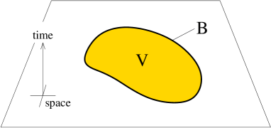
Figure 1: A hypersurface of equal time. The spacelike entropy bound attempts to relate the entropy in a spatial region, $V$, to the area of its boundary, $B$. This is not successful.

Let $V$ be a compact portion of a hypersurface of equal time in the spacetime ${\cal M}$. Let $S(V)$ be the entropy of all matter systems in $V$. Let $B$ be the boundary of $V$ and let $A$ be the area of the boundary of $V$. Then

$$S(V)\leq{A[B(V)]\over 4}.$$ (45)

IV.2 Inadequacies

The spacelike entropy bound is not a successful conjecture. Eq. (45) is contradicted by a large variety of counterexamples. We will begin by discussing two examples from cosmology. Then we will turn to the case of a collapsing star. Finally, we will expose violations of Eq. (45) even for all isolated, spherical, weakly gravitating matter systems.

IV.2.1 Closed spaces

It is hardly necessary to describe a closed universe in detail to see that it will lead to a violation of the spacelike holographic principle. It suffices to assume that the spacetime ${\cal M}$ contains a closed spacelike hypersurface, ${\cal V}$. (For example, there are realistic cosmological solutions in which ${\cal V}$ has the topology of a three-sphere.) We further assume that ${\cal V}$ contains a matter system that does not occupy all of ${\cal V}$, and that this system has non-zero entropy $S_{0}$.

Let us define the volume $V$ to be the whole hypersurface, except for a small compact region $Q$ outside the matter system. Thus, $S_{\rm matter}(V)=S_{0}>0$. The boundary $B$ of $V$ coincides with the boundary of $Q$. Its area can be made arbitrarily small by contracting $Q$ to a point. Thus one obtains $S_{\rm matter}(V)>A[B(V)])$, and the spacelike entropy bound, Eq. (45), is violated.

IV.2.2 The Universe

On large scales, the universe we inhabit is well approximated as a three-dimensional, flat, homogeneous and isotropic space, expanding in time. Let us pick one homogeneous hypersurface of equal time, ${\cal V}$. Its entropy content can be characterized by an average “entropy density”, $\sigma$, which is a positive constant on ${\cal V}$. Flatness implies that the geometry of ${\cal V}$ is Euclidean ${\mathbb{R}}^{3}$. Hence, the volume and area of a two-sphere grow in the usual way with the radius:

$$V={4\pi\over 3}R^{3},~{}~{}~{}A[B(V)]=4\pi R^{2}.$$ (46)

The entropy in the volume $V$ is given by

$$S_{\rm matter}(V)=\sigma V={\sigma\over 6\sqrt{\pi}}A^{3/2}.$$ (47)

Recall that we are working in Planck units. By taking the radius of the sphere to be large enough,

$$R\geq{3\over 4\sigma},$$ (48)

one finds a volume for which the spacelike entropy bound, Eq. (45), is violated (Fischler and Susskind, 1998).

IV.2.3 Collapsing star

Next, consider a spherical star with non-zero entropy $S_{0}$. Suppose the star burns out and undergoes catastrophic gravitational collapse. From an outside observer’s point of view, the star will form a black hole whose surface area will be at least $4S_{0}$, in accordance with the generalized second law of thermodynamics.

However, we can follow the star as it falls through its own horizon. From collapse solutions (see, e.g., Misner, Thorne, and Wheeler, 1973), it is known that the star will shrink to zero radius and end in a singularity. In particular, its surface area becomes arbitrarily small: $A\to 0$. By the second law of thermodynamics, the entropy in the enclosed volume, i.e., the entropy of the star, must still be at least $S_{0}$. Once more, the spacelike entropy bound fails (Easther and Lowe, 1999).

As in the previous two examples, this failure does not concern the spherical entropy bound, even though spherical symmetry may hold. We are considering a regime of dominant gravity, in violation of the assumptions of the spherical bound. In the interior of a black hole, both the curvature and the time-dependence of the metric are large.

IV.2.4 Weakly gravitating system

The final example is the most subtle. It shows that the spacelike entropy bound can be violated by the very systems for which the spherical entropy bound is believed to hold: spherical, weakly gravitating systems. This is achieved merely by a non-standard coordinate choice that breaks spherical symmetry and measures a smaller surface area.

Consider a weakly gravitating spherical thermodynamic system in asymptotically flat space. Note that this class includes most thermodynamic systems studied experimentally; if they are not spherical, one redefines their boundary to be the circumscribing sphere.

A coordinate-independent property of the system is its world volume, $W$. For a stable system with the spatial topology of a three-dimensional ball ($\mathbf{D}^{3}$), the topology of $W$ is given by ${\mathbb{R}}\times\mathbf{D}^{3}$ (Fig. 2).

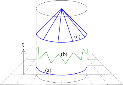
Figure 2: The worldvolume of a ball of gas, with one spatial dimension suppressed. (a) A time slice in the rest frame of the system is shown as a flat plane. It intersects the boundary of system on a spherical surface, whose area exceeds the system’s entropy. (b) In a different coordinate system, however, a time slice intersects the boundary on Lorentz-contracted surfaces whose area can be made arbitrarily small. Thus the spacelike entropy bound is violated. (c) The light-sheet of a spherical surface is shown for later reference (Sec. V.3.1). Light-sheets of wiggly surfaces may not penetrate the entire system (Sec. VII.3).—The solid cylinder depicted here can also be used to illustrate the conformal shape of Anti-de Sitter space (Sec. IX.2).

The volume of the ball of gas, at an instant of time, is geometrically the intersection of the world volume $W$ with an equal time hypersurface $t=0$:

$$V\equiv W\cap\{t=0\}.$$ (49)

The boundary of the volume $V$ is a surface $B$ given by

$$B=\partial W\cap\{t=0\}.$$ (50)

The time coordinate $t$, however, is not uniquely defined. One possible choice for $t$ is the proper time in the rest frame of the weakly gravitating system (Fig. 2a). With this choice, $V$ and $B$ are metrically a ball and a sphere, respectively. The area $A(B)$ and the entropy $S_{\rm matter}(V)$ were calculated in Sec. II.3.3 for the example of a ball of gas. They were found to satisfy the spacelike entropy bound, Eq. (45).

From the point of view of general relativity, there is nothing special about this choice of time coordinate. The laws of physics must be covariant, i.e., invariant under general coordinate transformations. Thus Eq. (45) must hold also for a volume $V^{\prime}$ associated with a different choice of time coordinate, $t^{\prime}$. In particular, one may choose the $t^{\prime}=$const hypersurface to be rippled like a fan. Then its intersection with $\partial W$, $B^{\prime}$, will be almost null almost everywhere, like the zigzag line circling the worldvolume in Fig. 2b. The boundary area so defined can be made arbitrarily small (Jacobson, 1999; Flanagan, Marolf, and Wald, 2000; Smolin, 2001). This construction has shown that a spherical system with non-zero entropy $S_{\rm matter}$ can be enclosed within a surface of area $A(B^{\prime})<S_{\rm matter}$, and the spacelike entropy bound, Eq. (45), is again violated.

How is this possible? After all, the spherical entropy bound should hold for this system, because it can be converted into a spherical black hole of the same area. However, this argument implicitly assumed that the boundary of a spherically symmetric system is a sphere (and therefore agrees with the horizon area of the black hole after the conversion). With the non-standard time coordinate $t^{\prime}$, however, the boundary is not spherically symmetric, and its area is much smaller than the final black hole area. (The latter is unaffected by slicing ambiguities because a black hole horizon is a null hypersurface.)

IV.3 Range of validity

In view of these problems, it is clear that the spacelike entropy bound cannot be maintained as a fully general conjecture holding for all volumes and areas in all spacetimes. Still, the spherical entropy bound, Eq. (24), clearly holds for many systems that do not satisfy its assumptions, suggesting that those assumptions may be unnecessarily restrictive.

For example, the earth is part of a cosmological spacetime that is not, as far as we know, asymptotically flat. However, the earth does not curve space significantly. It is well separated from other matter systems. On time and distance scales comparable to the earth’s diameter, the universe is effectively static and flat. In short, it is clear that the earth will obey the spacelike entropy bound.

The same argument can be made for the solar system, and even for the milky way. As we consider larger regions, however, the effects of cosmological expansion become more noticable, and the flat space approximation is less adequate. An important question is whether a definite line can be drawn. In cosmology, is there a largest region to which the spacelike entropy bound can be reliably applied? If so, how is this region defined? Or does the bound gradually become less accurate at larger and larger scales?

Let us consider homogeneous, isotropic universes, known as Friedmann-Robertson-Walker (FRW) universes (Sec. VII.1). Fischler and Susskind (1998) abandoned the spacelike formulation altogether (Sec. V.1). For adiabatic FRW universes, however, their proposal implied that the spacelike entropy bound should hold for spherical regions smaller than the particle horizon (the future light cone of a point at the big bang).

Restriction to the particle horizon turns out to be sufficient for the validity of the spacelike entropy bound in simple flat and open models; thus, the problem in Sec. IV.2.2 is resolved. However, it does not prevent violations in closed or collapsing universes. The particle horizon area vanishes when the light cone reaches the far end of a closed universe—this is a special case of the problem discussed in Sec. IV.2.1. An analogue of the problem of Sec. IV.2.3 can arise also. Generally, closed universes and collapsing regions exhibit the greatest difficulties for the formulation of entropy bounds, and many authors have given them special attention.

Davies (1988) and Brustein (2000) proposed a generalized second law for cosmological spacetimes. They suggested that contradictions in collapsing universes may be resolved by augmenting the area law with additional terms. Easther and Lowe (1999) argued that the second law of thermodynamics implies a holographic entropy bound, at least for flat and open universes, in regions not exceeding the Hubble horizon. Similar conclusions were reached by Veneziano (1999b), Kaloper and Linde (1999), and Brustein (2000).

Bak and Rey (2000a) argued that the relevant surface is the apparent horizon, defined in Sec. VII.1.2. This is a minor distinction for typical flat and open universes, but it avoids some of the difficulties with closed universes.

The arguments for bounds of this type return to the Susskind process, the gedankenexperiment by which the spherical entropy bound was derived (Sec. II.3.1). A portion of the universe is converted to a black hole; the second law of thermodynamics is applied. One then tries to understand what might prevent this gedankenexperiment from being carried out.

For example, regions larger than the horizon are expanding too rapidly to be converted to a black hole—they cannot be “held together” (Veneziano, 1999b). Also, if a system is already inside a black hole, it can no longer be converted to one. Hence, one would not expect the bound to hold in collapsing regions, such as the interior of black holes or a collapsing universe (Easther and Lowe, 1999; Kaloper and Linde, 1999).

This reasoning does expose some of the limitations of the spacelike entropy bound (namely those that are illustrated by the explicit counterexamples given in Sec. IV.2.1 and IV.2.3). However, it fails to identify sufficient conditions under which the bound is actually reliable. Kaloper and Linde (1999) give counterexamples to any statement of the type “The area of the particle (apparent, Hubble) horizon always exceeds the entropy enclosed in it” (Sec. VII.1.6).

In the following section we will introduce the covariant entropy bound, which is formulated in terms of light-sheets. In Sec. VII we will present evidence that this bound has universal validity. Starting from this general bound, one can find sufficient conditions under which a spacelike formulation is valid (Sec. VI.3.1, VII.1.7). However, the conditions themselves will involve the light-sheet concept in an essential way. Not only is the spacelike formulation less general than the light-sheet formulation; the range of validity of the former cannot be reliably identified without the latter.

We conclude that the spacelike entropy bound is violated by realistic matter systems. In cosmology, its range of validity cannot be intrinsically defined.

V The covariant entropy bound

In this section we present a more successful generalization of Eq. (24): the covariant entropy bound.

There are two significant formal differences between the covariant bound and the spacelike bound, Eq. (45). The spacelike formulation starts with a choice of spatial volume $V$. The volume, in turn, defines a boundary $B=\partial V$, whose area $A$ is then claimed to be an upper bound on $S(V)$, the entropy in $V$. The covariant bound proceeds in the opposite direction. A codimension 2 surface $B$ serves as the starting point for the construction of a codimension 1 region $L$. This is the first formal difference. The second is that $L$ is a null hypersurface, unlike $V$ which is spacelike.

More precisely, $L$ is a light-sheet. It is constructed by following light rays that emanate from the surface $B$, as long as they are not expanding. There are always at least two suitable directions away from $B$ (Fig. 3). When light rays self-intersect, they start to expand. Hence, light-sheets terminate at focal points.

The covariant entropy bound states that the entropy on any light-sheet of a surface $B$ will not exceed the area of $B$:

$$S[L(B)]\leq{A(B)\over 4}.$$ (51)

We will give a more formal definition at the end of this section.

Figure 3: The four null hypersurfaces orthogonal to a spherical surface $B$. The two cones $F_{1}$, $F_{3}$ have negative expansion and hence correspond to light-sheets. The covariant entropy bound states that the entropy on each light-sheet will not exceed the area of $B$. The other two families of light rays, $F_{2}$ and $F_{4}$, generate the skirts drawn in thin outline. Their cross-sectional area is increasing, so they are not light-sheets. The entropy of the skirts is not related to the area of $B$.—Compare this figure to Fig. 1.

We begin with some remarks on the conjectural nature of the bound, and we mention related earlier proposals. We will explain the geometric construction of light-sheets in detail, giving special attention to the considerations that motivate the condition of non-expansion ($\theta\leq 0$). We give a definition of entropy on light-sheets, and we discuss the extent to which the limitations of classical general relativity are inherited by the covariant entropy bound. We then summarize how the bound is formulated, applied, and tested. Parts of this section follow Bousso (1999a).

V.1 Motivation and background

There is no fundamental derivation of the covariant entropy bound. We present the bound because there is strong evidence that it holds universally in nature. The geometric construction is well-defined and covariant. The resulting entropy bound can be saturated, but no example is known where it is exceeded.

In Sec. VI.2 plausible relations between entropy and energy are shown to be sufficient for the validity of the bound. But these relations do not at present appear to be universal or fundamental. In special situations, the covariant entropy bound reduces to the spherical entropy bound, which is arguably a consequence of black hole thermodynamics. But in general, the covariant entropy bound cannot be inferred from black hole physics; quite conversely, the generalized second law of thermodynamics may be more appropriately regarded as a consequence of the covariant bound (Sec. VI.3.2).

The origin of the bound remains mysterious. As discussed in the introduction, this puzzle forms the basis of the holographic principle, which asserts that the covariant entropy bound betrays the number of degrees of freedom of quantum gravity (Sec. VIII).

Aside from its success, little motivation for a light-like formulation can be offered. Under the presupposition that some general entropy bound waits to be discovered, one is guided to light rays by circumstantial evidence. This includes the failure of the spacelike entropy bound (Sec. IV), the properties of the Raychaudhuri equation (Sec. VI.1), and the loss of a dynamical dimension in the light cone formulation of string theory (Sec. I.4).

Whatever the reasons, the idea that light rays might be involved in relating a region to its surface area—or, rather, relating a surface area to a light-like “region”—arose in discussions of the holographic principle from the beginning.

Susskind (1995b) suggested that the horizon of a black hole can be mapped, via light rays, to a distant, flat holographic screen, citing the focussing theorem (Sec. VI.1) to argue that the information thus projected would satisfy the holographic bound. Corley and Jacobson (1996) pointed out that the occurrence of focal points, or caustics, could invalidate this argument, but showed that one caustic-free family of light rays existed in Susskind’s example. They further noted that both past and future directed families of light rays can be considered.

Fischler and Susskind (1998) recognized that a light-like formulation is crucial in cosmological spacetimes, because the spacelike entropy bound fails. They proposed that any spherical surface $B$ in FRW cosmologies (see Sec. VII.1) be related to (a portion of) a light cone that comes from the past and ends on $B$. This solved the problem discussed in Sec. IV.2.2 for flat and open universes but not the problem of small areas in closed or recollapsing universes (see Secs. IV.2.1, IV.2.3).

The covariant entropy bound (Bousso, 1999a) can be regarded as a refinement and generalization of the Fischler-Susskind proposal. It can be applied in arbitrary spacetimes, to any surface $B$ regardless of shape, topology, and location. It considers all four null directions orthogonal to $B$ without prejudice. It introduces a new criterion, the contraction of light rays, both to select among the possible light-like directions and to determine how far the light rays may be followed. For any $B$, there will be at least two “allowed” directions and hence two light-sheets, to each of which the bound applies individually.

V.2 Light-sheet kinematics

Compared to the previously discussed bounds, Eqs. (24) and (45), the non-trivial ingredient of the covariant entropy bound lies in the concept of light-sheets. Given a surface, a light-sheet defines an adjacent spacetime region whose entropy should be considered. What has changed is not the formula, $S\leq A/4$, but the prescription that determines where to look for the entropy $S$ that enters that formula. Let us discuss in detail how light-sheets are constructed.

V.2.1 Orthogonal null hypersurfaces

A given surface $B$ possesses precisely four orthogonal null directions (Fig. 3). They are sometimes referred to as future directed ingoing, future directed outgoing, past directed ingoing, and past directed outgoing, though “in” and “out” are not always useful labels. Locally, these directions can be represented by null hypersurfaces $F_{1},\ldots,F_{4}$ that border on $B$. The $F_{i}$ are generated by the past and the future directed light rays orthogonal to $B$, on either side of $B$.

For example, suppose that $B$ is the wall of a (spherical) room in approximately flat space, as shown in Fig. 3, at $t=0$. (We must keep in mind that $B$ denotes a surface at some instant of time.) Then the future directed light rays towards the center of the room generate a null hypersurface $F_{1}$, which looks like a light cone. A physical way of describing $F_{1}$ is to imagine that the wall is lined with light bulbs that all flash up at $t=0$. As the light rays travel towards the center of the room they generate $F_{1}$.

Similarly, one can line the outside of the wall with light bulbs. Future directed light rays going to the outside will generate a second null hypersurface $F_{2}$. Finally, one can also send light rays towards the past. (We might prefer to think of these as arriving from the past, i.e., a light bulb in the center of the room flashed at an appropriate time for its rays to reach the wall at $t=0$.) In any case, the past directed light rays orthogonal to $B$ will generate two more null hypersurfaces $F_{3}$ and $F_{4}$.

In Fig. 3, the two ingoing cones $F_{1}$ and $F_{3}$, and the two outgoing “skirts”, $F_{2}$ and $F_{4}$, are easily seen to be null and orthogonal to $B$. However, the existence of four null hypersurfaces bordering on $B$ is guaranteed in Lorentzian geometry independently of the shape and location of $B$. They are always uniquely generated by the four sets of surface-orthogonal light rays.

At least two of the four null hypersurfaces $F_{1},\ldots,F_{4}$ will be selected as light-sheets, according to the condition of non-positive expansion discussed next.

V.2.2 Light-sheet selection

Let us return to the example where $B$ is the wall of a spherical room. If gravity is weak, one would expect that the area $A$ of $B$ will be a bound on the entropy in the room (Sec. II.3.1). Clearly, $A$ cannot be related in any way to the entropy in the infinite region outside the room; that entropy could be arbitrarily large. It appears that we should select $F_{1}$ or $F_{3}$ as light-sheets in this example, because they correspond to our intuitive notion of “inside”.

The question is how to generalize this notion. It is obvious that one should compare an area only to entropy that is in some sense “inside” the area. However, consider a closed universe, in which space is a three-sphere. As Sec. IV.2.1 has illustrated, we need a criterion that prevents us from considering the large part of the three-sphere to be “inside” a small two-sphere $B$.

What we seek is a local condition, which will select whether some direction away from $B$ is an inside direction. This condition should reduce to the intuitive, global notion—inside is where infinity is not—where applicable. An analogy in Euclidean space leads to a useful criterion, the contraction condition.

Figure 4: Local definition of “inside”. (a) Ingoing rays perpendicular to a convex surface in a Euclidean geometry span decreasing area. This motivates the following local definition. (b) Inside is the direction in which the cross-sectional area decreases ($A^{\prime}\leq A$). This criterion can be applied to light rays orthogonal to any surface. After light rays locally intersect, they begin to expand. Hence, light-sheets must be terminated at caustics.

Consider a convex closed surface $B$ of codimension one and area $A$ in flat Euclidean space, as shown in Fig. 4a. Now construct all the geodesics intersecting $B$ orthogonally. Follow each geodesic an infinitesimal proper distance $dl$ to one of the two sides of $B$. The set of points thus obtained will span a similarly shaped surface of area $A^{\prime}$. If $A^{\prime}<A$, let us call the chosen direction the “inside”. If $A^{\prime}>A$, we have gone “outside”.

Unlike the standard notion of “inside”, the contraction criterion does not depend on any knowledge of the global properties of $B$ and of the space it is embedded in. It can be applied independently to arbitrarily small pieces of the surface. One can always construct orthogonal geodesics and ask in which direction they contract. It is local also in the orthogonal direction; the procedure can be repeated after each infinitesimal step.

Let us return to Lorentzian signature, and consider a codimension 2 spatial surface $B$. The contraction criterion cannot be used to find a spatial region “inside” $B$. There are infinitely many different spacelike hypersurfaces $\Sigma$ containing $B$. Which side has contracting area could be influenced by the arbitrary choice of $\Sigma$.

However, the four null directions $F_{1},\ldots,F_{4}$ away from $B$ are uniquely defined. It is straightforward to adapt the contraction criterion to this case. Displacement by an infinitesimal spatial distance is meaningless for light rays, because two points on the same light ray always have distance zero. Rather, an appropriate analogue to length is the affine parameter $\lambda$ along the light ray (see the Appendix). Pick a particular direction $F_{i}$. Follow the orthogonal null geodesics away from $B$ for an infinitesimal affine distance $d\lambda$. The points thus constructed span a new surface of area $A^{\prime}$. If $A^{\prime}\leq A$, then the direction $F_{i}$ will be considered an “inside” direction, or light-sheet direction.

By repeating this procedure for $i=1,\ldots,4$, one finds all null directions that point to the “inside” of $B$ in this technical sense. Because the light rays generating opposite pairs of null directions (e.g., $F_{1}$ and $F_{4}$) are continuations of each other, it is clear that at least one member of each pair will be considered inside. If the light rays are locally neither expanding nor contracting, both members of a pair will be called “inside”. Hence, there will always be at least two light-sheet directions. In degenerate cases, there may be three or even four.

Mathematically, the contraction condition can be formulated thus:

$$\theta(\lambda)\leq 0~{}~{}~{}~{}\mbox{for}~{}\lambda=\lambda_{0},$$ (52)

where $\lambda$ is an affine parameter for the light rays generating $F_{i}$ and we assume that $\lambda$ increases in the direction away from $B$. $\lambda_{0}$ is the value of $\lambda$ on $B$. The expansion, $\theta$, of a family of light rays is discussed in detail in Sec. VI.1. It can be understood as follows. Consider a bunch of infinitesimally neighboring light rays spanning a surface area ${\cal A}$. Then

$$\theta(\lambda)\equiv\frac{d{\cal A}/d\lambda}{\cal A}.$$ (53)

As in the Euclidean analogy, this condition can be applied to each infinitesimal surface element separately and so is local. Crucially, it applies to open surfaces as well as to closed ones. This represents a significant advance in the generality of the formulation.

For oddly shaped surfaces or very dynamical spacetimes, it is possible for the expansion to change sign along some $F_{i}$. For example, this will happen for smooth concave surfaces in flat space. Because of the locality of the contraction criterion, one may split such surfaces into pieces with constant sign, and continue the analysis for each piece separately. This permits us to assume henceforth without loss of generality that the surfaces we consider have continuous light-sheet directions.

For the simple case of the spherical surface in Minkowski space, the condition (53) reproduces the intuitive answer. The area is decreasing in the $F_{1}$ and $F_{3}$ directions—the past and future directed light rays going to the center of the sphere. We will call any such surface, with two light-sheet directions on the same spatial side, normal.

In highly dynamical geometries, the expansion or contraction of space can be the more important effect on the expansion of light rays. Then it will not matter which spatial side they are directed at. For example, in an expanding universe, areas get small towards the past, because the big bang is approached. A sufficiently large sphere will have two past directed light-sheets, but no future directed ones. A surface of this type is called anti-trapped. Similarly, in a collapsing universe or inside a black hole, space can shrink so rapidly that both light-sheets are future directed. Surfaces with this property are trapped.

In a Penrose diagram (Appendix), a sphere is represented by a point. The four orthogonal null directions correspond to the four legs of an “X” centered on this point. Light-sheet directions can be indicated by drawing only the corresponding legs (Bousso 1999a). Normal, trapped, and anti-trapped surfaces are thus denoted by wedges of different orientation (see Figs. 5, 7a, and 8).

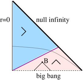
Figure 5: Penrose diagram for an expanding universe (a flat or open FRW universe, see Sec. VII.1). The thin curve is a slice of constant time. Each point in the interior of the diagram represents a sphere. The wedges indicate light-sheet directions. The apparent horizon (shown here for equation of state $p=\rho$) divides the normal spheres near the origin from the anti-trapped spheres near the big bang. The light-sheets of any sphere $B$ can be represented by inspecting the wedge that characterizes the local domain and drawing lines away from the point representing $B$, in the direction of the wedge’s legs.

V.2.3 Light-sheet termination

From now on we will consider only inside directions, $F_{j}$, where $j$ runs over two or more elements of $\{1,2,3,4\}$. For each $F_{j}$, a light-sheet is generated by the corresponding family of light rays. In the example of the spherical surface in flat space, the light-sheets are cones bounded by $B$, as shown in Fig. 3.

Strictly speaking, however, there was no particular reason to stop at the tip of the cone, where all light rays intersect. On the other hand, it would clearly be desastrous to follow the light rays arbitrarily far. They would generate another cone which would grow indefinitely, containing unbounded entropy. One must enforce, by some condition, that the light-sheet is terminated before this happens. In all but the most special cases, the light rays generating a light-sheet will not intersect in a single point, so the condition must be more general.

A suitable condition is to demand that the expansion be non-positive everywhere on the light-sheet, and not only near $B$:

$$\theta(\lambda)\leq 0,$$ (54)

for all values of the affine parameter on the light-sheet.

By construction (Sec. V.2.2) the expansion is initially negative or zero on any light-sheet. Raychaudhuri’s equation guarantees that the expansion can only decrease.. (This will be shown explicitly in Sec. VI.1.) The only way $\theta$ can become positive is if light rays intersect, for example at the tip of the light cone. However, it is not necessary for all light rays to intersect in the same point. By Eq. (53), the expansion becomes positive at any caustic, that is, any place where a light ray crosses an infinitesimally neighboring light ray in the light-sheet (Fig. 4b).

Thus, Eq. (54) operates independently of any symmetries in the setup. It implies that light-sheets end at caustics. In general, each light ray in a light-sheet will have a different caustic point, and the resulting caustic surfaces can be very complicated. The case of a light cone is special in that all light rays share the same caustic point at the tip. An ellipsoid in flat space will have a self-intersecting light-sheet that may contain the same object more than once (at two different times). Gravitational back-reaction of matter will make the caustic surfaces even more involved.

Non-local self-intersections of light rays do not lead to violations of the contraction condition, Eq. (54). That is, the light-sheet must be terminated only where a light ray intersects its neighbor, but not necessarily when it intersects another light ray coming from a different portion of the surface $B$. One can consider modifications of the light-sheet definition where any self-intersection terminates the light-sheet (Tavakol and Ellis, 1999; Flanagan, Marolf, and Wald, 2000). Since this modification can only make light-sheets shorter, it can weaken the resulting bound. However, in most applications, the resulting light-sheets are easier to calculate (as Tavakol and Ellis, in particular, have stressed) and still give useful bounds.

The condition, Eq. (54), subsumes Eq. (52), which applied only to the initial value of $\lambda$. It is satisfying that both the direction and the extent of light-sheets are determined by the same simple condition, Eq. (54).

V.3 Defining entropy

V.3.1 Entropy on a fixed light-sheet

The geometric construction of light-sheets is well-defined. But how is “the entropy on a light-sheet”, $S_{\rm matter}$, determined? Let us begin with an example where the definition of $S_{\rm matter}$ is obvious. Suppose that $B$ is a sphere around an isolated, weakly gravitating thermodynamic system. Given certain macroscopic constraints, for example an energy or energy range, pressure, volume, etc., the entropy of the system can be computed either thermodynamically, or statistically as the logarithm of the number of accessible quantum states.

To good approximation, the two light-sheets of $B$ are a past and a future light cone. Let us consider the future directed light-sheet. The cone contains the matter system completely (Fig. 2c), in the same sense in which a $t=\mbox{const}$ surface contains the system completely (Fig. 2a). A light-sheet is just a different way of taking a snapshot of a matter system—in light cone time. (In fact, this comes much closer to how the system is actually observed in practice.) Hence, the entropy on the light-sheet is simply given by the entropy of the matter system.

A more problematic case arises when the light-sheet intersects only a portion of an isolated matter system, or if there simply are no isolated systems in the spacetime. A reasonable (statistical) working definition was given by Flanagan, Marolf, and Wald (2000), who demanded that long wavelength modes which are not fully contained on the light-sheet should not be included in the entropy.

In cosmological spacetimes, entropy is well approximated as a continuous fluid. In this case, $S_{\rm matter}$ is the integral of the entropy density over the light-sheet (Secs. VI.2, VII.1).

One would expect that the gravitational field itself can encode information perturbatively, in the form of gravitational waves. Because it is difficult to separate such structure from a “background metric”, we will not discuss this case here.

We have formulated the covariant entropy bound for matter systems in classical geometry and have not made provisions for the inclusion of the semi-classical Bekenstein entropy of black holes. There is evidence, however, that the area of event horizons can be included in $S_{\rm matter}$. However, in this case the light-sheet must not be continued to the interior of the black hole. The Bekenstein entropy of the black hole already contains the information about objects that fell inside; it must not be counted twice (Sec. III.7).

V.3.2 Entropy on an arbitrary light-sheet

So far we have treated the light-sheet of $B$ as a fixed null hypersurface, e.g., in the example of an isolated thermodynamic system. Different microstates of the system, however, correspond to different distributions of energy. This is a small effect on average, but it does imply that the geometry of light-sheets will vary with the state of the system in principle.

In many examples, such as cosmological spacetimes, one can calculate light-sheets in a large-scale, averaged geometry. In this approximation, one can estimate $S_{\rm matter}$ while holding the light-sheet geometry fixed.

In general, however, one can at best hold the surface $B$ fixed, but not the light-sheet of $B$. We must consider $S_{\rm matter}$ to be the entropy on any light-sheet of $B$. Sec. VII.2.3, for example, discusses the collapse of a shell onto an apparent black hole horizon. In this example, a part of the spacetime metric is known, including $B$ and the initial expansions $\theta_{i}$ of its orthogonal light rays. However, the geometry to the future of $B$ is not presumed, and different configurations contributing to the entropy lead to macroscopically different future light-sheets.

In a static, asymptotically flat space the specification of a spherical surface reduces to the specification of an energy range. The enclosed energy must lie between zero and the mass of a black hole that fills in the sphere. Unlike most other thermodynamic quantities such as energy, however, the area of surfaces is well-defined in arbitrary geometries.

In the most general case, one may specify only a surface $B$ but no information about the embedding of $B$ in any spacetime. One is interested in the entropy of the “fundamental system” (Sec. III.2), i.e., the number of quantum states associated with the light-sheets of $B$ in any geometry containing $B$. This leaves too much freedom for Eq. (51) to be checked explicitly. The covariant entropy bound essentially becomes the full statement of the holographic principle (Sec. VIII) in this limit.

V.4 Limitations

Here we discuss how the covariant entropy bound is tied to a regime of approximately classical spacetimes with reasonable matter content. The discussion of the “species problem” (Sec. II.3.4) carries over without significant changes and will not be repeated.

V.4.1 Energy conditions

In Sec. II.3.3 we showed that the entropy of a ball of radiation is bounded by $A^{3/4}$, and hence is less than its surface area. For larger values of the entropy, the mass of the ball would exceed its radius, so it would collapse to form a black hole. But what if matter of negative energy was added to the system? This would offset the gravitational backreaction of the gas without decreasing its entropy. The entropy in any region could be increased at will while keeping the geometry flat.

This does not automatically mean that the holographic principle (and indeed, the generalized second law of thermodynamics) is wrong. A way around the problem might be to show that instabilities develop that will invalidate the setup we have just suggested. But more to the point, the holographic principle is expected to be a property of the real world. And to a good approximation, matter with negative mass does not exist in the real world.

Einstein’s general relativity does not restrict matter content, but tells us only how matter affects the shape of spacetime. Yet, of all the types of matter that could be added to a Lagrangian, few actually occur in nature. Many would have pathological properties or catastrophic implications, such as the instability of flat space.

In a unified theory underlying gravity and all other forces, one would expect that the matter content is dictated by the theory. String theory, for example, comes packaged with a particular field content in its perturbative limits. However, there are many physically interesting spacetimes that have yet to be described in string theory (Sec. IX.1), so it would be premature to consider only fields arising in this framework.

One would like to test the covariant entropy bound in a broad class of systems, but we are not interested whether the bound holds for matter that is entirely unphysical. It is reasonable to exclude matter whose energy density appears negative to a light ray, or which permits the superluminal transport of energy. In other words, let us demand the null energy condition as well as the causal energy condition. Both conditions are spelled out in the Appendix, Eqs. (132) and (133). They are believed to be satisfied classically by all physically reasonable forms of matter.

Negative energy density is generally disallowed by these conditions, with the exception of a negative cosmological constant. This is desirable, because a negative cosmological constant does not lead to instabilities or other pathologies. It may well occur in the universe, though it is not currently favored by observation. Unlike other forms of negative energy, a negative cosmological constant cannot be used to cancel the gravitational field of ordinary thermodynamic systems, so it should not lead to difficulties with the holographic principle.

Quantum effects can violate the above energy conditions. Casimir energy, for example, can be negative. However, the relation between the magnitude, size, and duration of such violations is severely constrained (see, e.g., Ford and Roman, 1995, 1997, 1999; Flanagan, 1997; Fewster and Eveson, 1998; Fewster, 1999; further references are found in Borde, Ford, and Roman, 2001). Even where they occur, their gravitational effects may be overcompensated by those of ordinary matter. It has not been possible so far to construct a counterexample to the covariant entropy bound using quantum effects in ordinary matter systems.

V.4.2 Quantum fluctuations

What about quantum effects in the geometry itself? The holographic principle refers to geometric concepts such as area, and orthogonal light rays. As such, it can be applied only where spacetime is approximately classical. This contradicts in no way its deep relation to quantum gravity, as inferred from the quantum aspects of black holes (Sec. II) and demonstrated by the AdS/CFT correspondence (Sec. IX.2).

In the real world, $\hbar$ is fixed, so the regime of classical geometry is generically found in the limit of low curvature and large distances compared to the Planck scale, Eq. (2). Setting $\hbar$ to $0$ would not only be unphysical; as Lowe (1999) points out, it would render the holographic bound, $Akc^{3}/4G\hbar$, trivial.

Lowe (1999) has argued that a naive application of the bound encounters difficulties when effects of quantum gravity become important. With sufficient fine tuning, one can arrange for an evaporating black hole to remain in equilibrium with ingoing radiation for an arbitarily long time. Consider the future directed outgoing light-sheet of an area on the black hole horizon. Lowe claims that this light-sheet will have exactly vanishing expansion and will continue to generate the horizon in the future, as it would in a classical spacetime. This would allow an arbitrarily large amount of ingoing radiation entropy to pass through the light-sheet, in violation of the covariant entropy bound.

If a light-sheet lingers in a region that cannot be described by classical general relativity without violating energy conditions for portions of the matter, then it is outside the scope of the present formulation of the covariant entropy bound. The study of light-sheets of this type may guide the exploration of semi-classical generalizations of the covariant entropy bound. For example, it may be appropriate to associate the outgoing Hawking radiation with a negative entropy flux on this light-sheet (Flanagan, Marolf, and Wald, 2000).

However, Bousso (2000a) argued that a violation of the covariant entropy bound has not been demonstrated in Lowe’s example. In any realistic situation small fluctuations in the energy density of radiation will occur. They are indeed inevitable if information is to be transported through the light-sheet. Thus the expansion along the light-sheet will fluctuate. If it becomes positive, the light-sheet must be terminated. If it fluctuates but never becomes positive, then it will be negative on average. In that case an averaged version of the focussing theorem implies that the light rays will focus within a finite affine parameter.

The focussing is enhanced by the $-\theta^{2}/2$ term in Raychaudhuri’s equation, (64), which contributes to focussing whenever $\theta$ fluctuates about zero. Because of these effects, the light-sheets considered by Lowe (1999) will not remain on the horizon, but will collapse into the black hole. New families of light rays continually move inside to generate the event horizon. It is possible to transport unlimited entropy through the black hole horizon in this case, but not through any particular light-sheet.

V.5 Summary

In any $D$-dimensional Lorentzian spacetime $M$, the covariant entropy bound can be stated as follows.

Let $A(B)$ be the area of an arbitrary $D-2$ dimensional spatial surface $B$ (which need not be closed). A $D-1$ dimensional hypersurface $L$ is called a light-sheet of $B$ if $L$ is generated by light rays which begin at $B$, extend orthogonally away from $B$, and have non-positive expansion,

$$\theta\leq 0,$$ (55)

everywhere on $L$. Let $S$ be the entropy on any light-sheet of $B$. Then

$$S\leq{A(B)\over 4}.$$ (56)

Let us restate the covariant entropy bound one more time, in a constructive form most suitable for applying and testing the bound, as we will in Sec. VII.

1. Pick any $D-2$ dimensional spatial surface $B$, and determine its area $A(B)$. There will be four families of light rays projecting orthogonally away from $B$: $F_{1}\ldots F_{4}$.

2. Usually additional information is available, such as the macroscopic spacetime metric everywhere or in a neighborhood of $B$. Then the expansion $\theta$ of the orthogonal light rays can be calculated for each family. Of the four families, at least two will not expand ($\theta\leq 0$). Determine which.

3. Pick one of the non-expanding families, $F_{j}$. Follow each light ray no further than to a caustic, a place where it intersects with neighboring light rays. The light rays form a $D-1$ dimensional null hypersurface, a light-sheet $L(B)$.

4. Determine the entropy $S[L(B)]$ of matter on the light-sheet $L$, as described in Sec. V.3.1.

5. The quantities $S[L(B)]$ and $A(B)$ can then be compared. The covariant entropy bound states that the entropy on the light-sheet will not exceed a quarter of the area: $S[L(B)]\leq\frac{A(B)}{4}$. This must hold for any surface $B$, and it applies to each non-expanding null direction, $F_{j}$, separately.

The first three steps can be carried out most systematically by using geometric tools which will be introduced at the beginning of Sec. VI.1. In simple geometries, however, they often require little more than inspection of the metric.

The light-sheet construction is well-defined in the limit where geometry can be described classically. It is conjectured to be valid for all physically realistic matter systems. In the absence of a fundamental theory with definite matter content, the energy conditions given in Sec. V.4.1 approximately delineate the boundaries of an enormous arena of spacetimes and matter systems, in which the covariant entropy bound implies falsifiable, highly non-trivial limitations on information content.

In particular, the bound is predictive and can be tested by observation, in the sense that the entropy and geometry of real matter systems can be determined (or, as in the case of large cosmological regions, at least estimated) from experimental measurements.

VI The dynamics of light-sheets

Entropy requires energy. In Sec. III.5, this notion gave us some insight into a mechanism underlying the spherical entropy bound. Let us briefly repeat the idea. When one tries to excite too many degrees of freedom in a spherical region of fixed boundary area $A$, the region becomes very massive and eventually forms a black hole of area no larger than $A$. Because of the second law of thermodynamics, this collapse must set in before the entropy exceeds $A/4$. Of course, it can be difficult to verify this quantitatively for a specific system; one would have to know its detailed properties and gravitational back-reaction.

In this section, we identify a related mechanism underlying the covariant entropy bound. Entropy costs energy, energy focusses light, focussing leads to the formation of caustics, and caustics prevent light-sheets from going on forever. As before, the critical link in this argument is the relation between entropy and energy. Quantitatively, it depends on the details of specific matter systems and cannot be calculated in general. Indeed, this is one of the puzzles that make the generality of the covariant entropy bound so striking.

In many situations, however, entropy can be approximated by a local flow of entropy density. With plausible assumptions on the relation between the entropy and energy density, which we review, Flanagan, Marolf, and Wald (2000) proved the covariant entropy bound.

We also present the spacelike projection theorem, which identifies conditions under which the covariant bound implies a spacelike bound (Bousso, 1999a).

VI.1 Raychaudhuri’s equation and the focussing theorem

A family of light rays, such as the ones generating a light-sheet, is locally characterized by its expansion, shear, and twist, which are defined as follows.

Let $B$ be a surface of $D-2$ spatial dimensions, parametrized by coordinates $x^{\alpha}$, $\alpha=1,\ldots,D-2$. Pick one of the four families of light rays $F_{1},\ldots,F_{4}$ that emanate from $B$ into the past and future directions to either side of $B$ (Fig. 3). Each light ray satisfies the equation for geodesics (Appendix):

$$\frac{dk^{a}}{d\lambda}+\Gamma^{a}_{~{}bc}k^{b}k^{c}=0,$$ (57)

where $\lambda$ is an affine parameter. The tangent vector $k^{a}$ is defined by

$$k^{a}=\frac{dx^{a}}{d\lambda}$$ (58)

and satisfies the null condition $k^{a}k_{a}=0$. The light rays generate a null hypersurface $L$ parametrized by coordinates $(x^{\alpha},\lambda)$. This can be rephrased as follows. In a neighborhood of $B$, each point on $L$ is unambiguously defined by the light ray on which it lies ($x^{\alpha}$) and the affine distance from $B$ ($\lambda$).

Let $l^{a}$ be the null vector field on $B$ that is orthogonal to $B$ and satisfies $k^{a}l_{a}=-2$. (This means that $l^{a}$ has the same time direction as $k^{a}$ and is tangent to the orthogonal light rays constructed on the other side of $B$.) The induced $D-2$ dimensional metric on the surface $B$ is given by

$$h_{ab}=g_{ab}+\frac{1}{2}\left(k_{a}l_{b}+k_{b}l_{a}\right).$$ (59)

In a similar manner, an induced metric can be found for all other spatial cross-sections of $L$.

The null extrinsic curvature,

$$B_{ab}=h^{c}_{~{}a}h^{d}_{~{}b}\nabla_{c}k_{d},$$ (60)

contains information about the expansion, $\theta$, shear, $\sigma_{ab}$, and twist, $\omega_{ab}$, of the family of light rays, $L$:

$$\theta = h^{ab}B_{ab},$$ (61)

$$\sigma_{ab} = \frac{1}{2}\left(B_{ab}+B_{ba}\right)-\frac{1}{D-2}\theta h_{ab},$$ (62)

$$\omega_{ab} = \frac{1}{2}\left(B_{ab}-B_{ba}\right).$$ (63)

Note that all of these quantities are functions of $(x^{\alpha},\lambda)$.

At this point, one can inspect the initial values of $\theta$ on $B$. Where they are positive, one must discard $L$ and choose a different null direction for the construction of a light-sheet.

The Raychaudhuri equation describes the change of the expansion along the light rays:

$$\frac{d\theta}{d\lambda}=-\frac{1}{D-2}\theta^{2}-\sigma_{ab}\sigma^{ab}+\omega_{ab}\omega^{ab}-8\pi T_{ab}k^{a}k^{b}.$$ (64)

For a surface-orthogonal family of light rays, such as $L$, the twist vanishes (Wald, 1984). The final term, $-T_{ab}k^{a}k^{b}$, will be non-positive if the null energy condition is satisfied by matter, which we assume (Sec. V.4.1). Then the right hand side of the Raychaudhuri equation is manifestly non-positive. It follows that the expansion never increases.

By solving the differential inequality

$$\frac{d\theta}{d\lambda}\leq-\frac{1}{D-2}\theta^{2},$$ (65)

one arrives at the focussing theorem: If the expansion of a family of light rays takes the negative value $\theta_{1}$ at any point $\lambda_{1}$, then $\theta$ will diverge to $-\infty$ at some affine parameter $\lambda_{2}\leq\lambda_{1}+{D-2\over|\theta_{1}|}$.

The divergence of $\theta$ indicates that the cross-sectional area is locally vanishing, as can be seen from Eq. (53). As discussed in Sec. V.2.3, this is a caustic point, at which infinitesimally neighboring light rays intersect.

By construction, the expansion on light-sheets is zero or negative. If it is zero, the focussing theorem does not apply. For example, suppose that $B$ is a portion of the $xy$ plane in Minkowski space: $z=t=0,~{}~{}x^{2}+y^{2}\leq 1$. Then each light-sheet is infinitely large, with everywhere vanishing expansion: $z=\pm t,~{}~{}x^{2}+y^{2}\leq 1$. However, this is correct only if the spacetime is exactly Minkowski, with no matter or gravitational waves. In this case the light-sheets contain no entropy in any case, so their infinite size leads to no difficulties with the covariant entropy bound.

If a light-sheet encounters any matter (or more precisely, if $T_{ab}k^{a}k^{b}>0$ anywhere on the light-sheet), then the light rays will be focussed according to Eq. (64). Then the focussing theorem applies, and it follows that the light rays will eventually form caustics, forcing the light-sheet to end. This will happen even if no further energy is encountered by the light rays, though it will occur sooner if there is additional matter.

If we accept that entropy requires energy, we thus see at a qualitative level that entropy causes light rays to focus. Thus, the presence of entropy hastens the termination of light-sheets. Quantitatively, it appears to do so at a sufficient rate to protect the covariant entropy bound, but slowly enough to allow saturation of the bound. This is seen in many examples, including those studied in Sec. VII. The reason for this quantitative behavior is not yet fundamentally understood. (This just reformulates, in terms of light-sheet dynamics, the central puzzle laid out in the introduction and reiterated in Sec. VIII.)

VI.2 Sufficient conditions for the covariant entropy bound

Flanagan, Marolf, and Wald (2000; henceforth in this section, FMW) showed that the covariant entropy bound is always satisfied if certain assumptions about the relation between entropy density and energy density are made. In fact, they proved the bound under either one of two sets of assumptions. We will state these assumptions and discuss their plausibility and physical significance. We will not reproduce the two proofs here.

The first set of conditions are no easier to verify, in any given spacetime, than the covariant entropy bound itself. Light-sheets have to be constructed, their endpoints found, and entropy can be defined only by an analysis of modes. The first set of conditions should therefore be regarded as an interesting reformulation of the covariant entropy bound, which may shed some light on its relation to the Bekenstein bound, Eq. (11).

The second set of conditions involves relations between locally defined energy and entropy densities only. As long as the entropy content of a spacetime admits a fluid approximation, one can easily check whether these conditions hold. In such spacetimes, the second FMW theorem obviates the need to construct all light-sheets and verify the bound for each one.

Neither set of conditions is implied by any fundamental law of physics. The conditions do not apply to some physically realistic systems (which nevertheless obey the covariant entropy bound). Furthermore, they do not permit macroscopic variations of spacetime, precluding a verification of the bound in its strongest sense (Sec. V.3.2).

Thus, as FMW point out, the two theorems do not constitute a fundamental explanation of the covariant entropy bound. By eliminating a large class of potential counter-examples, they do provide important evidence for the validity of the covariant entropy bound. The second set can significantly shortcut the verification of the bound in cosmological spacetimes. Moreover, the broad validity of the FMW hypotheses may itself betray an aspect of an underlying theory.

VI.2.1 The first FMW theorem

The first set of assumptions is

• Associated with each light-sheet $L$ in spacetime there is an entropy flux 4-vector $s^{a}_{L}$ whose integral over $L$ is the entropy flux through $L$.

• The inequality

  $$\left|s_{L}^{a}k^{a}\right|\leq{\pi}(\lambda_{\infty}-\lambda)T_{ab}k^{a}k^{b}$$ (66)

  holds everywhere on $L$. Here $\lambda_{\infty}$ is the value of the affine parameter at the endpoint of the light-sheet.

The entropy flux vector $s_{L}^{a}$ is defined non-locally by demanding that only modes that are fully captured on $L$ contribute to the entropy on $L$. Modes that are partially contained on $L$ do not contribute. This convention recognizes that entropy is a non-local phenomenon. It is particularly useful when light-sheets penetrate a thermodynamic system only partially, as discussed in Sec. V.3.1.

This set of assumptions can be viewed as a kind of “light ray equivalent” of Bekenstein’s bound, Eq. (11), with the affine parameter playing the role of the circumferential radius. However, it is not clear whether one should expect this condition to be satisfied in regions of dominant gravity. Indeed, it does not apply to some weakly gravitating systems (Sec. VI.3.2).

FMW were actually able to prove a stronger form of the covariant entropy bound from the above hypotheses. Namely, suppose that the light-sheet of a surface of area $A$ is constructed, but the light rays are not followed all the way to the caustics. The resulting light-sheet is, in a sense, shorter than necessary, and one would expect that the entropy on it, $S$, will not saturate the bound. The final area spanned by the light rays, $A^{\prime}$, will be less than $A$ but non-zero (Fig. 4b).

FMW showed, with the above assumptions, that a tightened bound results in this case:

$$S\leq\frac{A-A^{\prime}}{4}.$$ (67)

Note that this expression behaves correctly in the limit where the light-sheet is maximized [$A^{\prime}\to 0$; one recovers Eq. (56)] and minimized ($A^{\prime}\to A$; there is no light-sheet and hence no entropy).

The strengthened form, Eq. (67), of the covariant entropy bound, Eq. (56), appears to have broad, but not completely general validity (Sec. VI.3.2).

VI.2.2 The second FMW theorem

Through a rather non-trivial proof, FMW showed that the covariant entropy bound can also be derived from a second set of assumptions, namely:

• The entropy content of spacetime is well approximated by an absolute entropy flux vector field $s^{a}$.

• For any null vector $k^{a}$, the inequalities

  $$(s_{a}k^{a})^{2} \leq {1\over 16\pi}T_{ab}k^{a}k^{b},$$ (68)

  $$\left|k^{a}k^{b}\nabla_{a}s_{b}\right| \leq {\pi\over 4}T_{ab}k^{a}k^{b}$$ (69)

  hold at everywhere in the spacetime.

These assumptions are satisfied by a wide range of matter systems, including Bose and Fermi gases below the Planck temperature. It is straightforward to check that all of the adiabatically evolving cosmologies investigated in Sec. VII.1 conform to the above conditions. Thus, the second FMW theorem rules out an enormous class of potential counterexamples, obviating the hard work of calculating light-sheets. (We will find light-sheets in simple cosmologies anyway, both in order to gain intuition about how the light-sheet formulation works in cosmology, and also because this analysis is needed for the discussion of holographic screens in Sec. IX.3.)

Generally speaking, the notion of an entropy flux assumes that entropy can be treated as a kind of local fluid. This is often a good approximation, but it ignores the non-local character of entropy and does not hold at a fundamental level.

VI.3 Relation to other bounds and to the GSL

VI.3.1 Spacelike projection theorem

We have seen in Sec. IV.2 that the spacelike entropy bound does not hold in general. Taking the covariant entropy bound as a general starting point, one may derive other, more limited formulations, whose regimes of validity are defined by the assumptions entering the derivation. Here we use the light-sheet formulation to recover the spacelike entropy bound, Eq. (45), along with precise conditions under which it holds. By imposing further conditions, even more specialized bounds can be obtained; an example valid for certain regions in cosmological spacetimes is discussed in Sec. VII.1.7 below.

Figure 6: Spacelike projection theorem. If the surface $B$ has a complete future directed light-sheet $L$, then the spacelike entropy bound applies to any spatial region $V$ enclosed by $B$.

Spacelike projection theorem (Bousso, 1999a). Let $B$ be a closed surface. Assume that $B$ permits at least one future directed light-sheet $L$. Moreover, assume that $L$ is complete, i.e., $B$ is its only boundary (Fig. 6). Let $S(V)$ be the entropy in a spatial region $V$ enclosed by $B$ on the same side as $L$. Then

$$S(V)\leq S(L)\leq\frac{A}{4}.$$ (70)

Proof. Independently of the choice of $V$ (i.e., the choice of a time coordinate), all matter present on $V$ will pass through $L$. The second law of thermodynamics implies the first inequality, the covariant entropy bound implies the second.

What is the physical significance of the assumptions made in the theorem? Suppose that the region enclosed by $B$ is weakly gravitating. Then we may expect that all assumptions of the theorem are satisfied. Namely, if $B$ did not have a future directed light-sheet, it would be anti-trapped—a sign of strong gravity. If $L$ had other boundaries, this would indicate the presence of a future singularity less than one light-crossing time from $B$—again, a sign of strong gravity.

Thus, for a closed, weakly gravitating, smooth surface $B$ we may expect the spacelike entropy bound to be valid. In particular, the spherical entropy bound, deemed necessary for the validity of the GSL in the Susskind process, follows from the covariant bound. This can be see by inspecting the assumptions in (Sec. II.3), which guarantee that the conditions of the spacelike projection theorem are satisfied.

VI.3.2 Generalized second law and Bekenstein bound

In fact, FMW showed that the covariant bound implies the GSL directly for any process of black hole formation, such as the Susskind process (Sec. II.3.1).

Consider a surface $B$ of area $A$ on the event horizon of a black hole. The past directed ingoing light rays will have non-positive expansion; they generate a light-sheet. The light-sheet contains all the matter that formed the black hole. The covariant bound implies that $S_{\rm matter}\leq A(B)/4=S_{\rm BH}$. Hence, the generalized second law is satisfied for the process in which a black hole is newly formed from matter.

Next, let us consider a more general process, the absorption of a matter system by an existing black hole. This includes the Geroch process (Sec. II.2.1). Does the covariant bound also imply the GSL in this case?

Consider a surface $B$ on the event horizon after the matter system, of entropy $S_{\rm matter}$, has fallen in, and follow the past-ingoing light-rays again. The light-rays are focussed by the energy momentum of the matter. “After” proceeding through the matter system, let us terminate the light-sheet. Thus the light-sheet contains precisely the entropy $S_{\rm matter}$. The rays will span a final area $A^{\prime}$ (which is really the initial area of the event horizon before the matter fell in).

According to an outside observer, the Bekenstein entropy of the black hole has increased by $(A-A^{\prime})/4$, while the matter entropy $S_{\rm matter}$ has been lost. According to the “strengthened form” of the covariant entropy bound considered by FMW, Eq. (67), the total entropy has not decreased. The original covariant bound, Eq. (56), does not by itself imply the generalized second law of thermodynamics, Eq. (5), in this process.

Eq. (67) can also be used to derive a version of Bekenstein’s bound, Eq. (11)—though, unfortunately, a version that is too strong. Consider the light-sheet of an approximately flat surface of area $A$, bounding one side of a rectangular thermodynamic system. With suitable time-slicing, the surface can be chosen to have vanishing null expansion, $\theta$.

With assumptions on the average energy density and the equation of state, Raychaudhuri’s equation can be used to estimate the final area $A^{\prime}$ of the light-sheet where it exits the opposite side of the matter system. The strengthened form of the covariant entropy bound, Eq. (67) then implies the bound given in Eq. (23). However, for very flat systems this bound can be violated (Sec. II.2.2)!

Hence, (67) cannot hold in the same generality that is claimed for the original covariant entropy bound, Eq. (56). However, the range of validity of Eq. (67) does appear to be extremely broad. In view of the significance of its implications, it will be important to better understand its scope.

We conclude that the covariant entropy bound implies the spherical bound in its regime of validity, defines a range of validity for the spacelike bound, and implies the GSL for black hole formation processes. The strengthened form of the covariant bound given by FMW, Eq. (67), implies the GSL for absorption processes and, under suitable assumptions, yields Bekenstein’s bound [though in a form that demonstates that Eq. (67) cannot be universally valid].

The result of this section suggest that the holographic principle (Sec. VIII) will take a primary role in the complex of ideas we have surveyed. It may come to be viewed as the logical origin not only of the covariant entropy bound, but also of more particular laws that hold under suitable conditions, such as the spherical entropy bound, Bekenstein’s bound, and the generalized second law of thermodynamics.

VII Applications and examples

In this section, the covariant entropy bound is applied to a variety of matter systems and spacetimes. We demonstrate how the light-sheet formulation evades the various difficulties encountered by the spacelike entropy bound (Sec. IV.2).

We apply the bound to cosmology and verify explicitly that it is satisfied in a wide class of universes. No violations are found during the gravitational collapse of a star, a shell, or the whole universe, though the bound can be saturated.

VII.1 Cosmology

VII.1.1 FRW metric and entropy density

Friedmann-Robertson-Walker (FRW) metrics describe homogeneous, isotropic universes, including, to a good degree of approximation, the portion we have seen of our own universe. Often the metric is expressed in the form

$$ds^{2}=-dt^{2}+a^{2}(t)\left(\frac{dr^{2}}{1-kr^{2}}+r^{2}d\Omega^{2}\right).$$ (71)

We will find it more useful to use the conformal time $\eta$ and the comoving coordinate $\chi$:

$$d\eta={dt\over a(t)},~{}~{}~{}d\chi={dr\over\sqrt{1-kr^{2}}}.$$ (72)

In these coordinates the FRW metric takes the form

$$ds^{2}=a^{2}(\eta)\left[-d\eta^{2}+d\chi^{2}+f^{2}(\chi)d\Omega^{2}\right].$$ (73)

Here $k=-1$, $0$, $1$ and $f(\chi)=\sinh\chi$, $\chi$, $\sin\chi$ correspond to open, flat, and closed universes respectively. Relevant Penrose diagrams are shown in Figs. 5 and 7a.

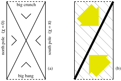
Figure 7: (a) Penrose diagram for a closed FRW universe filled with pressureless dust. The three-sphere time slices are represented by horizontal lines (not shown). Two apparent horizons divide the diagram into four wedge domains: normal spheres are found near the poles, trapped (anti-trapped) spheres near the big bang (big crunch). (b) The construction of a global holographic screen (Sec. IX.3) proceeds by foliating the spacetime into a stack of light cones. The information on each slice can be stored on the maximal sphere, which lies on the apparent horizon.

In cosmology, the entropy is usually described by an entropy density $\sigma$, the entropy per physical volume:

$$S(V)=\int_{V}d^{3}x\sqrt{h}\,\sigma.$$ (74)

For FRW universes, $\sigma$ depends only on time. We will assume, for now, that the universe evolves adiabatically. Thus, the physical entropy density is diluted by cosmological expansion:

$$\sigma(\eta)={s\over a(\eta)^{3}}.$$ (75)

The comoving entropy density $s$ is constant in space and time.

VII.1.2 Expansion and apparent horizons

Let us verify that the covariant entropy bound is satisfied for each light-sheet of any spherical surface $A$. The first step is to identify the light-sheet directions. We must classify each sphere as trapped, normal, or anti-trapped (Sec. V.2.2). Let us therefore compute the initial expansion of the four families of light rays orthogonal to an arbitrary sphere characterized by some value of $(\eta,\chi)$.

We take the affine parameter to agree locally with $\pm 2\eta$ and use Eq. (53). Differentiation with respect to $\eta$ ($\chi$) is denoted by a dot (prime). Instead of labelling the families $F_{1},\ldots,F_{4}$, it will be more convenient to use the notation $(\pm\pm)$, where the first sign refers to the time ($\eta$) direction of the light rays and the second sign denotes whether they are directed at larger or smaller values of $\chi$.

For the future directed families one finds

$$\theta_{+\pm}={\dot{a}\over a}\pm{f^{\prime}\over f}.$$ (76)

The expansion of the past directed families is given by

$$\theta_{-\pm}=-{\dot{a}\over a}\pm{f^{\prime}\over f}.$$ (77)

Note that the first term in Eq. (76) is positive when the universe expands and negative if it contracts. The term diverges when $a\to 0$, i.e., near singularities. The second term is given by $\cot\chi$ ($1/\chi$; $\coth\chi$) for a closed (flat; open) universe. It diverges at the origin ($\chi\to 0$), and for a closed universe it also diverges at the opposite pole ($\chi\to\pi$).

The signs of the four quantities $\theta_{\pm\pm}$ depend on the relative strength of the two terms. The quickest way to classify surfaces is to identify marginal spheres, where the two terms are of equal magnitude.

The apparent horizon is defined geometrically as a sphere at which at least one pair of orthogonal null congruences have zero expansion. It satisfies the condition

$${\dot{a}\over a}=\pm{f^{\prime}\over f},$$ (78)

which can be used to identify its location $\chi_{\rm AH}(\eta)$ as a function of time. There is one solution for open and flat universes. For a closed universe, there are generally two solutions, which are symmetric about the equator [$\chi_{{\rm AH}^{\prime}}(\eta)=\pi-\chi_{\rm AH}(\eta)$].

The proper area of the apparent horizon is given by

$$A_{\rm AH}(\eta)=4\pi a(\eta)^{2}f[\chi_{\rm AH}(\eta)]^{2}={4\pi a^{2}\over\left({\dot{a}\over a}\right)^{2}+k}.$$ (79)

Using Friedmann’s equation,

$${\dot{a}^{2}\over a^{2}}=\frac{8\pi\rho a^{2}}{3}-k,$$ (80)

one finds

$$A_{\rm AH}(\eta)={3\over 2\rho(\eta)},$$ (81)

where $\rho$ is the energy density of matter.

At any time $\eta$, the spheres that are smaller than the apparent horizon,

$$A<A_{\rm AH},$$ (82)

are normal. (See the end of Sec. V.2.2 for the definitions of normal, trapped, and anti-trapped surfaces.) Because the second term $f^{\prime}/f$ dominates in the expressions for the expansion, the cosmological evolution has no effect on the light-sheet directions. The two light-sheets will be a past and a future directed family going to the same spatial side. In a flat or open universe, they will be directed towards $\chi=0$ (Fig. 5). In a closed universe, the light-sheets of a normal sphere will be directed towards the nearest pole, $\chi=0$ or $\chi=\pi$ (Fig. 7a).

For spheres greater than the apparent horizon

$$A>A_{\rm AH},$$ (83)

the cosmological term $\dot{a}/a$ dominates in the expressions for the expansion. Then there are two cases. Suppose that $\dot{a}>0$, i.e., the universe is expanding. Then the spheres are anti-trapped. Both light-sheets are past directed, as indicated by a wedge opening to the bottom in the Penrose diagram. If $A>A_{\rm AH}$ and $\dot{a}<0$, then both future directed families will have negative expansion. This case describes trapped spheres in a collapsing universe. They are denoted by a wedge opening to the top (Fig. 7a).

VII.1.3 Light-sheets vs. spatial volumes

We have now classified all spherical surfaces in all FRW universes according to their light-sheet directions. Before proceeding to a detailed calculation of the entropy contained on the light-sheets, we note that the violations of the spacelike entropy bound identified in Secs. IV.2.1 and IV.2.2 do not apply to the covariant bound.

The area of a sphere at $\eta_{0},\chi_{0}$ is given by

$$A(\eta_{0},\chi_{0})=4\pi a(\eta_{0})^{2}f(\chi_{0})^{2}.$$ (84)

To remind ourselves that the spacelike entropy bound fails in cosmology, let us begin by comparing this area to the entropy enclosed in the spatial volume $V(\chi_{0})$ defined by $\chi\leq\chi_{0}$ at equal time $\eta=\eta_{0}$. With our assumption of adiabaticity, this depends only on $\chi_{0}$:

$$S[V(\chi_{0})]=4\pi s\int_{0}^{\chi_{0}}d\chi f(\chi)^{2}.$$ (85)

For a flat universe [$f(\chi)=\chi$], the area grows like $\chi_{0}^{2}$ but the entropy grows like $\chi_{0}^{3}$. Thus, $S[V(\chi_{0})]>A$ for sufficiently large $\chi_{0}$. (This was pointed out earlier in Sec. IV.2.2.) For a closed universe ($f(\chi)=\sin\chi$), $\chi$ ranges only from $0$ to $\pi$. $S[V(\chi_{0})]$ is monotonically increasing in this range, but $A\to 0$ for $\chi_{0}\to\pi$. Again, one has $S[V(\chi_{0})]>A$. This is a special case of the problem discussed in Sec. IV.2.1.

Why don’t light-sheets run into the same difficulties? Consider first a large sphere in a flat universe (Fig. 5). The future-ingoing light rays cover the same amount of entropy as the enclosed spatial volume. However, for spheres greater than the apparent horizon, the future-ingoing light rays are expanding and hence do not form a light-sheet. Only past directed light-sheets are permitted. The past-ingoing light rays, for example, will proceed towards the origin. However, if the sphere is greater than the particle horizon ($\chi>\eta$), they will terminate at the big bang ($\eta=0$) and will not get all the way to $\chi=0$. Instead of a comoving ball $0\leq\chi^{\prime}\leq\chi$, they will sweep out only a shell of width $\eta$: $\chi-\eta\leq\chi^{\prime}\leq\chi$. Thus the entropy to area ratio does not diverge for large $\chi$, but approaches a constant value.

Small spheres ($A<A_{\rm AH}$) in a closed universe (Fig. 7a) permit only light-sheets that are directed to the smaller enclosed region. The light rays directed towards the larger portion of the universe will be initially expanding and hence do not form light-sheets. Both in the flat and the closed case, we see that the $\theta\leq 0$ contraction condition is of crucial importance.

VII.1.4 Solutions with fixed equation of state

The matter content of FRW universes is most generally described by a perfect fluid, with stress tensor

$$T^{a}_{~{}b}=\mbox{diag}(-\rho,p,p,p).$$ (86)

Let us assume that the pressure $p$ and energy density $\rho$ are related by a fixed equation of state

$$p=w\rho.$$ (87)

Our universe and many other more general solutions can be pieced together from solutions obtained via this ansatz, because the transitions between different effective equations of state are very rapid.

For most of its lifetime, our universe was dominated by pressureless dust and hence was characterized by $w=0$. The early universe was dominated by radiation, which is described by $w={1\over 3}$. A cosmological constant, which may have been present at very early times and perhaps again today, corresponds to $w=-1$.

With this ansatz for the matter content and the FRW ansatz for the metric, Einstein’s equation can be solved. This determines the scale factor in Eq. (73):

$$a(\eta)=a_{0}\left[f({\eta\over q})\right]^{q},$$ (88)

where

$$q={2\over 1+3w},$$ (89)

and $f$ is the $\sin$ (the identity, $\sinh$) for a closed (flat, open) universe, as in Eq. (73). From Eq. (78) it follows that an apparent horizon is located at

$$\chi_{\rm AH}(\eta)={\eta\over q}$$ (90)

in all cases. An additional mirror horizon lies at $\pi-{\eta\over q}$ in the closed case.

Having established the light-sheet directions as a function of $t$ and $r$, we will now check whether the covariant entropy bound is satisfied on all light-sheets. The present treatment concentrates on flat and closed ($k=0,1$) universes with $w\geq 0$. However, we will quote results for $w<0$, i.e., negative pressure (Kaloper and Linde, 1999), which involves additional subtleties. We will also comment on the inflationary case ($w=-1$). We omit the open universes ($k=-1$) because they do not give rise to qualitatively new features (Fischler and Susskind, 1998). Bousso (1999a) discusses closed universes in detail. The main additional features beyond the flat case are covered in Secs. VII.1.3 and VII.2. We will comment on the inflationary case ($w=-1$) separately.

VII.1.5 Flat universe

Let us consider all possible light-sheets of all spherical areas ($0<\chi<\infty$) at the time $\eta$ in a flat FRW universe,

$$A(\eta,\chi)=4\pi a(\eta)^{2}\chi^{2}.$$ (91)

If $\chi\leq\chi_{\rm AH}(\eta)$, the sphere is normal, and the light-sheet directions are ($+-$) and ($--$). If $\chi\geq\chi_{\rm AH}$, the sphere is anti-trapped, with light-sheets ($-+$) and ($--$) (Fig. 5).

We begin with the future-ingoing ($+-$) light rays. They contract towards the origin and generate a conical light-sheet whose coordinates $(\chi^{\prime},\eta^{\prime})$ obey

$$\chi^{\prime}+\eta^{\prime}=\chi+\eta,$$ (92)

This light-sheet contains the comoving entropy in the region $0\leq\chi^{\prime}\leq\chi$, which is given by

$$S_{+-}={4\pi\over 3}s\chi^{3}.$$ (93)

The ratio of entropy to area,

$${S_{+-}\over A}={s\chi\over 3a(\eta)^{2}},$$ (94)

is maximized by the outermost normal surface at any given time $\eta$, the sphere on the apparent horizon. Thus we obtain the bound

$${S_{+-}\over A}\leq{s\chi_{\rm AH}(\eta)\over 3a(\eta)^{2}}.$$ (95)

The past-ingoing ($--$) light-sheet of any surface with $\chi<\eta$ also reaches a caustic at $\chi=0$. If $\chi>\eta$, then the light-sheet is truncated instead by the big bang singularity at $\eta=0$. Then it will contain the comoving entropy in the region $\chi-\eta\leq\chi^{\prime}\leq\chi$. The entropy to area ratio is given by

$${S_{--}\over A}={s\,\eta\over a(\eta)^{2}}\left(1-{\eta\over\chi}+{\eta^{2}\over 3\chi^{2}}\right).$$ (96)

This ratio is maximized for large spheres ($\chi\to\infty$), yielding the bound

$${S_{--}\over A}\leq{s\,\eta\over a(\eta)^{2}}$$ (97)

for the ($--$) light-sheets at time $\eta$.

Finally, we must consider the past-outgoing ($-+$) light-sheet of any surface with $\chi>\chi_{\rm AH}$. It is truncated by the big bang singularity and contains the entropy within $\chi\leq\chi^{\prime}\leq\chi+\eta$. The ratio of the entropy to the area,

$${S_{-+}\over A}={s\,\eta\over a(\eta)^{2}}\left(1+{\eta\over\chi}+{\eta^{2}\over 3\chi^{2}}\right),$$ (98)

is maximized for the smallest possible value of $\chi$, the apparent horizon. We find the bound

$${S_{-+}\over A}\leq{s\,\eta\over a(\eta)^{2}}\left(1+{\eta\over\chi_{\rm AH}}+{\eta^{2}\over 3\chi_{\rm AH}^{2}}\right).$$ (99)

We now use the solution for fixed equation of state, setting $a_{0}=1$ for convenience:

$$a(\eta)=\left({\eta\over q}\right)^{q},~{}~{}~{}\chi_{\rm AH}(\eta)={\eta\over q}.$$ (100)

Up to factors of order unity, the bounds for all three types of light-sheets at time $\eta$ agree:

$${S\over A}\leq s\,\eta^{1-2q}.$$ (101)

Note that one Planck distance corresponds to the comoving coordinate distance $\Delta\chi=a(\eta)^{-1}$. At the Planck time, $\eta\sim a(\eta)\sim O(1)$. Hence, $s$ is roughly the amount of entropy contained in a single Planck volume at one Planck time after the big bang. This is the earliest time and shortest distance scale one can hope to discuss without a full quantum gravity description. It is reasonable to assume that a Planck volume contains no more than one bit of information:

$$s\lesssim 1.$$ (102)

Eq. (101) then implies that the covariant entropy bound, Eq. (56), is satisfied at the Planck time. Moreover, the bound will continue to be satisfied by all light-sheets of all spheres at later times ($\eta>1$), if $q\geq{1\over 2}$. In terms of the parameter $w$, this corresponds to the condition

$$w\leq 1.$$ (103)

This result was obtained by Fischler and Susskind (1998) who also assumed $w\geq 0$.

Kaloper and Linde (1999) showed more generally that the entropy bound will be satisfied at all times if $-1<w\leq 1$, provided that the bound is satisfied at the Planck time. The case $w=-1$ corresponds to de Sitter space, in which there is no initial singularity. Since a cosmological constant does not carry entropy, the bound is trivially satisfied in this case. In summary, all light-sheets of all surfaces in any flat FRW universe with equation of state satisfying

$$-1\leq w\leq 1$$ (104)

satisfy the covariant entropy bound, Eq. (56).

This condition is physically very reasonable. It follows from the causal energy condition, which prohibits the superluminal flow of energy. We assumed in Sec. V.4.1 that this condition holds along with the null energy condition. The definitions of all relevant energy conditions are reviewed in the Appendix.

VII.1.6 Non-adiabatic evolution and mixed equations of state

So far, we have assumed that the universe evolves adiabatically. In order to relax this assumption, one generally has to abandon the FRW solution given above and find the exact geometry describing a cosmology with increasing entropy. However, the global solution will not change significantly if we rearrange matter on scales smaller than the apparent horizon.

Consider the future-ingoing light-sheet of the present apparent horizon, $L_{+-}[\eta_{0},\chi_{\rm AH}(\eta_{0})]$. All entropy we generate using the matter available to us inside the apparent horizon, will have to pass through this light-sheet. An efficient way to generate entropy is to form black holes. Building on a related discussion by Bak and Rey (2000a), Bousso (1999a) showed that the highest entropy is obtained in the limit where all matter is converted into a few big black holes. In this limit, $S_{+-}/A[\eta_{0},\chi_{\rm AH}(\eta_{0})]$ approaches $1/4$ from below. Hence the covariant bound is satisfied and can be saturated.

According to the inflationary model of the early universe (see, e.g., Linde, 1990), a different non-adiabatic process occurred at the end of inflation. At the time of reheating, matter is produced and a large amount of entropy is generated. One might be concerned that the holographic principle is violated by inflation (Easther and Lowe, 1999), or that it places severe constraints on acceptable models (Kalyana Rama and Sarkar, 1999).

Before inflation ended, however, there was almost no entropy. Hence, all past directed light-sheets can be truncated at the reheating surface, $\eta=\eta_{\rm reheat}$. The energy density at reheating is expected to be significantly below the Planck density. The light-sheets will be cut shorter than in our above discussion, which assumed that standard cosmology extended all the way back to the Planck era. Hence, inflation leads to no difficulties with the holographic principle.

Kaloper and Linde (1999) studied a particularly interesting cosmology, a flat FRW universe with ordinary matter, $w_{1}\geq 0,\rho_{1}>0$, as well as a small negative cosmological constant, $w_{2}=-1,\rho_{2}<0$. The universe starts matter dominated, but the cosmological constant eventually takes over the evolution. It slows down and eventually reverses the expansion. In a time symmetric fashion, matter eventually dominates and the universe ends in a future singularity.

The Kaloper-Linde universe provides a tough testing ground for proposals for a cosmological holographic principle. As in any flat FRW universe, spacelike holography breaks down for sufficiently large surfaces. Moreover, as in any collapsing universe, this occurs even if one restricts to surfaces within the particle horizon, or the Hubble horizon. Most interestingly, the “apparent horizon” proposal of Bak and Rey (2000a) fails in this cosmology. This can be understood by applying the spacelike projection theorem to cosmology, as we discuss next.

The holographic principle in anisotropic models was discussed by Fischler and Susskind (1998) and by Cataldo et al. (2001). Inhomogeneous universes have been considered by Tavakol and Ellis (1999); see also Wang, Abdallah, and Osada (2000).

VII.1.7 A cosmological corollary

Let us return to a question first raised in Sec. IV.3. What is the largest volume in a cosmological spacetime to which the spacelike holographic principle can be applied? The spacelike projection theorem (Sec. VI.3.1) guarantees that the spacelike entropy bound will hold for surfaces that admit a future directed, complete light-sheet. Let us apply this to cosmology. Surfaces on or within the apparent horizon are normal and hence admit a future directed light-sheet. However, the completeness condition is not trivial and must be demanded separately. In the Kaloper-Linde universe, for example, the future light-sheets of sufficiently late surfaces on the apparent horizon are truncated by the future singularity.

We thus arrive at the following corollary to the spacelike projection theorem (Bousso, 1999a): The area of any sphere within the apparent horizon exceeds the entropy enclosed in it, if the future light-sheet of the sphere is complete.

VII.2 Gravitational collapse

Any argument for an entropy bound based on the generalized second law of thermodynamics must surely become invalid in a collapse regime. When a system is already inside its own Schwarzschild radius, it can no longer be converted into a black hole of equal surface area.

Indeed, the example of the collapsing star (Sec. IV.2.3), and the conclusions reached by various analyses of collapsing universes (Sec. IV.3) would seem to discourage hopes of finding a non-trivial holographic entropy bound that continues to hold in regions undergoing gravitational collapse. Surprisingly, to the extent that it has been tested, the covariant entropy bound does remain valid in such regions.

Whenever possible, the validity of the bound is most easily verified by showing that a given solution satisfies the local hypotheses of Flanagan, Marolf, and Wald (2000). Otherwise, light-sheets must be found explicitly.

Ideally, one would like to investigate systems with high entropy, in dynamical, collapsing spacetime regions. Generically, such regions will be extremely inhomogeneous, which makes the practical calculation of light-sheets difficult. However, one should keep in mind that other proposals for general entropy bounds, such as the spacelike entropy bound, are quickly invalidated by simple, easily tractable counterexamples that make use of gravitational collapse.

It is remarkable, from this point of view, that the covariant bound has not met its demise by any of the standard collapse solutions that are readily available in the literature. To illustrate how the covariant bound evades violation, we will review its application to two simple examples, a collapsing star and a closed universe.

We will also consider a particular setup that allows the calculation of light-sheets deep inside a black hole formed by the collapse of a spherical shell. In this example one has good quantitative control over the collapse of a system of arbitrarily high entropy.

VII.2.1 Collapsing universe

Let us begin with a very simple example, the adiabatic recollapse of a closed FRW universe. In this case the recollapsing phase is just the time-reversal of the expanding phase. The light-sheet directions are similarly reversed (Fig. 7a). Small spheres near the poles are normal, but larger spheres, which are anti-trapped during expansion will be trapped during collapse. Their light-sheets are future directed and hence are typically truncated by the future (big crunch) singularity.

Because the solution is symmetric under time reversal, the validity of the covariant entropy bound in the collapse phase follows from its validity in the expanding phase. The latter can be verified straightforwardly. For anti-trapped spheres, the calculation (Fischler and Susskind, 1998) is similar to the analysis of the flat case (Sec. VII.1.5). For small spheres one needs to pay special attention to choosing the correct inside directions (see Sec. VII.1.3).

VII.2.2 Collapsing star

Next, we return to the collapsing star of Sec. IV.2.3. Why don’t the arguments demonstrating the break-down of other entropy bounds extend to the covariant entropy bound?

The metric in and around a collapsing star is well described by the Oppenheimer-Snyder solution (Misner, Thorne, and Wheeler, 1973). In this solution, the star is modelled by a suitable portion of a collapsing closed FRW universe. That is, one considers the coordinate range

$$0\leq\chi\leq\chi_{0},~{}~{}\eta>q{\pi\over 2},$$ (105)

in the metric of Eq. (73). Here, $q$ depends on the equation of state in the star according to Eq. (89). Also, $\chi_{0}<\pi/2$, so that the star does not overclose the universe. Outside the star, space is empty. Birkhoff’s theorem dictates that the metric will be given by a portion of the Schwarzschild solution, Eq. (12).

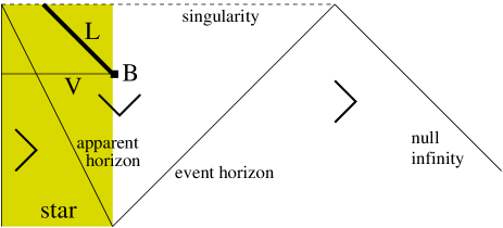
Figure 8: Penrose diagram of a collapsing star (shaded). At late times, the area of the star’s surface becomes very small ($B$). The enclosed entropy (in the spatial region $V$) stays finite, so that the spacelike entropy bound is violated. The covariant entropy bound avoids this difficulty because only future directed light-sheets are allowed. $L$ is truncated by the future singularity; it does not contain the entire star.

The corresponding Penrose diagram is shown in Fig. 8. The light-sheet directions are obtained from the corresponding portions of the Penrose diagrams for the closed universe (Fig. 7a) and for the Schwarzschild solution. At sufficiently late times, the apparent horizon reaches the surface of the star. At this moment, the star forms a black hole. The surface of the star is trapped at all later times. Hence, it admits only future directed light-sheets near the future singularity.

According to Eq. (84), the surface area of the star is given by

$$A(\chi_{0},\eta)=A_{\rm max}\left(\sin{\eta\over q}\right)^{q}.$$ (106)

Recall that $q$ is positive and of order unity for realistic equations of state. At the time of maximum expansion, $A=A_{\rm max}\equiv 4\pi a_{0}^{2}\sin^{2}\chi_{0}$. The future singularity corresponds to the time $\eta=q\pi$.

Let $B$ be the star’s surface at a time $\eta_{0}>q\pi-\chi_{0}$. The future directed ingoing light-sheet will be truncated by the future singularity at $\chi=\chi_{0}-(q\pi-\eta_{0})$, i.e., it will not traverse the star completely (Fig. 8). Hence, it will not contain the full entropy of the star. For very late times, $\eta_{0}\to\pi$, the surface area approaches zero, $A(\chi_{0},\eta_{0})\to 0$. The spacelike entropy bound is violated, $S(V)>A(B)$, because the entropy of the star does not decrease (Sec. IV.2.3). But the entropy $S(L)$ on the ingoing light-sheet, $L$, vanishes in this limit, because $L$ probes only a shallow outer shell, rather than the complete star.

Light-sheet truncation by future singularities is but one of several mechanisms that conspire to protect the covariant entropy bound during gravitational collapse (see Bousso, 1999a).

VII.2.3 Collapsing shell

Consider a small black hole of radius $r_{0}=2m$. In the future of the collapse event that formed this black hole, the apparent black hole horizon is a null hypersurface with spacelike, spherical cross-sections of area $A=4\pi r_{0}^{2}$.

Let us pick a particular sphere $B$ of area $A$ on the apparent horizon. By definition, the expansion of the past directed ingoing and the future directed outgoing light rays vanishes near $B$, so both are allowed light-sheet directions.

The former light-sheet contains all of the infalling matter that formed the black hole, with entropy $S_{\rm orig}$. The covariant entropy bound, in this case, is the statement of the generalized second law: the horizon entropy, $A/4$, is greater than the lost matter entropy, $S_{\rm orig}$. The future directed ingoing light rays will be contracting. They will contain entropy $S_{\rm orig}$ or less, so the covariant bound is satisfied once more.

We will be interested in the future directed outgoing light-sheet, $L$. It will continue to generate the apparent horizon of the black hole. Indeed, if no more matter ever enters the black hole, this apparent horizon coincides with the event horizon, and the light-sheet will continue forever at zero expansion.

Suppose, however, that more matter eventually falls into the black hole. When this happens, the apparent horizon moves out to a larger value $r>r_{0}$. (It will be generated by a new set of light rays that were formerly expanding.) The light-sheet $L$, however, will begin to collapse, according to Eq. (64). The covariant entropy bound predicts that the light rays will reach a singularity, or a caustic, before encountering more entropy than $A/4$.

This is a remarkable prediction. It claims that one cannot collapse more entropy through a (temporary) black hole horizon than it already has. This claim has been tested (Bousso, 1999a). Here we summarize only the method and results.

Far outside the black hole, one can assemble a shell of matter concentric with the black hole. By choosing the initial radius of this shell to be sufficiently large, one can suppress local gravitational effects and give the shell arbitary total mass, $M$, and width, $w$.

Let us assume that the shell is exactly spherically symmetric, even at the microscopic level. This suppresses the deflection of radial light rays into angular directions, rendering the eventual calculation of $L$ tractable. Moreover, it permits an estimate of the entropy of the shell.

In weakly gravitating systems, Bekenstein’s bound, Eq. (11), has much empirical support (Bekenstein, 1981, 1984; Schiffer and Bekenstein, 1989). There is independent evidence that the bound is always obeyed and can be nearly saturated by realistic, weakly gravitating matter systems.

Because all excitations are carried by radial modes, the shell can be divided along radial walls. This yields several weakly gravitating systems of largest length scale $w$. To each, Bekenstein’s bound applies. After reassembling the shell, one finds that its total entropy is bounded by

$$S\leq 2\pi Mw.$$ (107)

In principle, there are no restrictions on either $M$ or $w$, so the amount of entropy that can be collapsed onto the black hole is unlimited.

Now consider the adiabatic collapse of the shell. When the inner surface of the shell has shrunk to area $A$, the shell will first be reached by the light rays generating $L$. As the light rays penetrate the collapsing shell, they are focussed by the shell’s stress tensor. Their expansion becomes negative. Eventually they reach a caustic.

In order to violate the bound with a shell of large entropy, one would like to ensure that all of the shell’s entropy, $S$, will actually be contained on $L$. Thus, one should demand that the light rays must not reach a caustic before they have fully crossed the shell and reemerged on the outer surface of the shell.

Inspection of the collapse solution, however, reveals that this requirement restricts the shell’s mass and width,

$$Mw\leq r_{0}^{2}/2.$$ (108)

By Eq. (107), this also limits the entropy of the shell:

$$S\leq\pi r_{0}^{2}={A\over 4}.$$ (109)

The entropy on the light-sheet $L$ may saturate the covariant bound, but it will not violate it.

VII.3 Nearly null boundaries

In Sec. IV.2.4 it was shown that any isolated, weakly gravitating matter system can be surrounded with a closed surface of arbitarily small area, in violation of the spacelike entropy bound, Eq. (45).

In order to capture the key advantage of the light-sheet formulation, Eq. (56), we find it simplest to consider a square-shaped system occupying the region $0\leq x,y\leq a$ in 2+1 dimensional Minkowski space; $t$ is the time coordinate in the system’s rest frame (Fig. 9a). The boundary length of the system at $t=0$ is

$$A_{0}=4a.$$ (110)

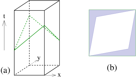
Figure 9: (a) A square system in 2+1 dimensions, surrounded by a surface $B$ of almost vanishing length $A$. (b) [Here the time dimension is projected out.] The light-sheet of $B$ intersects only with a negligible (shaded) fraction of the system.

Let us define a new boundary $B$ by a zig-zag curve consisting of the following four segments: $y=0$, $t=\beta x$ for $0\leq x\leq a$; $x=a$, $t=\beta(a-y)$ for $0\leq y\leq a$; $y=a$, $t=\beta(a-x)$ for $0\leq x\leq a$; and $x=0$, $t=\beta y$ for $0\leq y\leq a$. This can be regarded as the boundary of the system in some non-standard time-slicing. Its length is Lorentz-contracted relative to the boundary in the rest frame:

$$A(B)=A_{0}\sqrt{1-\beta^{2}}.$$ (111)

The length of $B$ vanishes in the limit as $\beta\to 1$.

The future-ingoing light-sheet $L(B)$ can be computed by piecing together the light-sheets of all four segments. The light-sheet of the first segment is obtained by translating the segment in the direction $(1,\beta,\sqrt{1-\beta^{2}})$. (It is instructive to verify that this generates an orthogonal null hypersurface of vanishing expansion. The curvature of spacetime is neglected in order to isolate the effect of “wiggling” the boundary.) For $\beta^{2}>{1\over 2}$, this light-sheet covers a fraction $\frac{\sqrt{1-\beta^{2}}}{2\beta}$ of the total system (Fig. 9b). The light-sheets of the other segments are similarly computed.

To leading order in $(1-\beta)$, the total fraction of the system covered by $L(B)$,

$${V(\beta)\over V_{0}}=\frac{2\sqrt{1-\beta^{2}}}{\beta},$$ (112)

vanishes at the same rate as the boundary length.

The future-ingoing light-sheet is not complete in this case; it has boundaries running through the interior of the system. Hence, the assumptions of the spacelike projection theorem are not satisfied. (This is not just an artifact of the sharp edges of $B$. If $B$ was smoothed at the edges, it would contain a segment on which only past directed light rays would be contracting. Thus, $B$ would not admit a future directed light-sheet everywhere, and the spacelike projection theorem would still not apply.)

VIII The holographic principle

VIII.1 Assessment

The previous sections have built a strong case for a holographic principle.

• The covariant entropy bound is well-defined (Sec. V). The light-sheet construction establishes a precise relation between surfaces and adjacent hypersurfaces. The area of the former must be compared to the entropy contained on the latter. Thus the bound is testable, in an arena limited only by the range of semi-classical gravity, the approximate framework we are compelled to use until a general quantum theory of gravity becomes available. Like any law of physics, it can of course be tested only to the extent that the relevant quantities and constructs (here, area, light-sheets, and entropy) are practically computable. But importantly, the bound will not become ill-defined in a regime which is otherwise physically well-understood.

• The bound has been examined and found to hold in a wide range of examples, some of which we reviewed in Sec. VII. No physically realistic counterexample has been found. This is remarkable especially in view of the ease with which the general validity of some alternative proposals can be excluded (Sec. IV).

• The bound is non-trivial. Naively one would expect the maximal entropy to grow with the volume of spatial regions. Instead, it is set by the area of surfaces.

• The bound refers to statistical entropy. Since it involves no assumptions about the microscopic properties of matter, it places a fundamental limit on the number of degrees of freedom in nature.

• The bound is not explained by other laws of physics that are presently known. Unlike its less general predecessors (e.g., the spherical entropy bound, Sec. II.3), the covariant bound cannot be regarded merely as a consequence of black hole thermodynamics. Arguments involving the formation of black holes cannot explain an entropy bound whose scope extends to the deep interior of black holes and to cosmology.—We conclude that the bound is an imprint of a more fundamental theory.

• Yet, the covariant bound is closely related to the black hole entropy and the generalized second law, long considered important clues to quantum gravity. Though the bound does not itself follow from thermodynamics, it implies other bounds which have been argued to be necessary for upholding the second law (Sec. VI.3). We also note that the bound essentially involves the quantum states of matter.—We conclude that the fundamental theory responsible for the bound unifies matter, gravity, and quantum mechanics.

• The bound relates information to a single geometric quantity (area). The bound’s simplicity, in addition to its generality, makes the case for its fundamental significance compelling.—We conclude that the area of any surface $B$ measures the information content of an underlying theory describing all possible physics on the light-sheets of $B$.

VIII.2 Formulation

Let us combine the three conclusions drawn above (in italics) and formulate the holographic principle (Bousso, 1999a,b).

The covariant entropy bound is a law of physics which must be manifest in an underlying theory. This theory must be a unified quantum theory of matter and spacetime. From it, Lorentzian geometries and their matter content must emerge in such a way that the number of independent quantum states describing the light-sheets of any surface $B$ is manifestly bounded by the exponential of the surface area:

$${\cal N}[L(B)]\leq e^{A(B)/4}.$$ (113)

(See Secs. I.2, V.5 for notation.)

Implicit in the phrase “quantum states” is the equivalence, in quantum theory, of the logarithm of the dimension ${\cal N}$ of Hilbert space and the amount of information stored in the quantum system. As it is not obvious that quantum mechanics will be primary in a unified theory, a more neutral formulation of the holographic principle may be preferable:

$N$, the number of degrees of freedom (or the number of bits times $\ln 2$) involved in the description of $L(B)$, must not exceed $A(B)/4$.

VIII.3 Implications

The holographic principle implies a radical reduction in the number of degrees of freedom we use to describe nature. It exposes quantum field theory, which has degrees of freedom at every point in space, as a highly redundant effective description, in which the true number of degrees of freedom is obscured (Sec. III.5).

The holographic principle challenges us to formulate a theory in which the covariant entropy bound is manifest. How can a holographic theory be constructed? Physics appears to be local to a good approximation. The number of degrees of freedom in any local theory is extensive in the volume. Yet, the holographic principle dictates that the information content is in correspondence with the area of surfaces. How can this tension be resolved? There appear to be two main lines of approach, each casting the challenge in a different form.

One type of approach aims to retain locality. A local theory could be rendered holographic if an explicit gauge invariance was identified, leaving only as many physical degrees of freedom as dictated by the covariant entropy bound. The challenge, in this case, is to implement such an enormous and rather peculiar gauge invariance.

For example, ’t Hooft (1999, 2000a, 2001a,b,c) is pursuing a local approach in which quantum states arise as limit cycles of a classical dissipative system (see also van de Bruck, 2000). The emergence of an area’s worth of physical degrees of freedom has yet to be demonstrated in such models.

A second type of approach regards locality as an emergent phenomenon without fundamental significance. In this case, the holographic data are primary. The challenge is not only to understand their generation and evolution. One must also explain how to translate underlying data, in a suitable regime, into a classical spacetime inhabited by local quantum fields. In a successful construction, the geometry must be shaped and the matter distributed so as to satisfy the covariant entropy bound. Because holographic data are most naturally associated with the area of surfaces, a serious difficulty arises in understanding how locality can emerge in this type of approach.

The AdS/CFT correspondence (Sec. IX.2) lends credence to the second type of approach. However, because it benefits from several peculiarities of the asympotically AdS universes to which it applies (Sec. IX.3), it has offered little help to researchers pursuing such approaches more broadly.

Some of the proposals and investigations discussed in Secs. IX.4 and IX.5 can be associated to the second type.

Which type of approach one prefers will depend, to a great extent, on which difficulty one abhors more: the elimination of most degrees of freedom, or the recovery of locality. The dichotomy is hardly strict; the two alternatives are not mutually exclusive. A successful theory may admit several equivalent formulations, thus reconciling both points of view.

Since light-sheets are central to the formulation of the holographic principle, one would expect null hypersurfaces to play a primary role in the classical limit of an underlying holographic theory (though this may not be apparent in descriptions of weakly time-dependent geometries; see Sec. IX.2).

IX Holographic screens and holographic theories

We will begin this section by discussing which aspects of the holographic principle have already been realized in string theory. We assess how general the class of universes is in which the holographic principle is thus implemented. In this context, we will present the most explicit example of a holographic theory presently known. The AdS/CFT correspondence defines quantum gravity—albeit in a limited set of spacetimes. Anti-de Sitter space contains a kind of holographic screen, a distant hypersurface on which holographic data can be stored and evolved forward using a conformal field theory.

We will then review the construction of holographic screens in general spacetimes, including those without boundary. Using light-sheets, it is always possible to find such screens. However, a theory that generally describes the generation and evolution of holographic data remains elusive. The structure of screens offers some clues about the difficulties that must be addressed. We will list a number of approaches.

We will also discuss the application of the covariant entropy bound to universes with positive vacuum energy. In this class of spacetimes the holographic principle appears to place a particularly strong constraint on an underlying description.

IX.1 String theory and the holographic principle

IX.1.1 A work in progress

String theory naturally produces a unified quantum description of gravity and matter fields. Its framework has proven self-consistent in remarkably non-trivial ways, given rise to powerful mathematical structures, and solved numerous physical problems. One might wonder what the holographic principle is still needed for. If a good theory is available, why search further? What is left to do?

String theory has developed in an unconventional way. It began as a formula whose physical interpretation in terms of strings was understood only later. The theory was first misunderstood as a description of hadrons, and only later recognized as a quantum theory of gravity. It forms part of a rigid mathematical structure whose content and physical implications continue to be explored.

String theory has yet to address many of the most pressing questions one would like to ask of a fundamental theory. These include phenomenological issues: Why does the world have four large dimensions? What is the origin of the stardard model? How is supersymmetry broken? More importantly, there are conceptual difficulties. It is unclear how the theory can be applied to realistic cosmological spacetimes, and how it might describe most black holes and singularities of general relativity.

String theory’s most notable recent successes hinged on the discovery of a new set of objects in the theory, D-branes (Polchinksi, 1995). Before D-branes, string theory’s list of open questions was longer than it is today. This serves as a reminder that unsolved problems need not signal the failure of string theory. Neither should they be dismissed as mere technical difficulties. Instead, they may indicate that there are still crucial parts of the theory that have not been discovered.

There is little evidence that string theory, in its current form, represents more than a small portion, or a limiting case, of a bigger theoretical structure. Nor is it clear that the exploration of this structure will continue to proceed most efficiently from within.

An intriguing success of the covariant entropy bound is its validity in highly dynamical geometries, whose description has proven especially difficult in string theory. This suggests that the holographic principle may offer useful guidance to the further development of the theory.

Its present limitations prevent string theory from explaining the general validity of the covariant entropy bound. The theory is not under control in many situations of interest, for example when supersymmetry is broken. Moreover, many solutions of physical relevance, including most of the examples in this text, do not appear to be admitted by string theory in its current form.

IX.1.2 Is string theory holographic?

These restrictions aside, one may ask whether the holographic principle is manifest in string theory. Let us consider, for a moment, only spacetimes that string theory can describe, and in which the holographic principle is also well-defined (i.e., geometry is approximately classical). Is the number of degrees of freedom involved in the string theory description set by the area of surfaces?

In perturbative string theory, the holographic principle is only partly realized. Effects associated with holography include the independence of the wave function on the longitudinal coordinate in the light cone frame, and the growth of the size of states with their momentum (see the reviews cited in Sec. I.4; Thorn, op. cit.; Klebanov and Susskind, 1988; Susskind, 1995b; see also Susskind, 1995a).

A number of authors have studied the extent to which string theory exhibits the non-locality implied by the holographic principle (Lowe, Susskind, and Uglum, 1994; Lowe et al., 1995). These investigations are closely related to the problem of understanding of the unitarity of black hole evaporation from the point of view of string theory, in particular through the principle of black hole complementarity (Sec. III.7).

The entropy bound of one bit per Planck area, however, is not explicit in perturbative string theory. Susskind (1995b) showed that the perturbative expansion breaks down before the bound is violated (see also Banks and Susskind, 1996). One would expect the holographic principle to be fully manifest only in a non-perturbative formulation of the theory.

Since the holographic principle was conceived, non-perturbative definitions of string theory have indeed become available for two special classes of spacetimes. Remarkably, in the AdS/CFT correspondence, the number of degrees of freedom agrees manifestly with the holographic principle, as we discuss below. In Matrix theory (Banks et al., 1997) the corresponding arguments are somewhat less precise. This is discussed, e.g., by Bigatti and Susskind (1997), and by Banks (1998, 1999), where further references can be found.

The holographic principle may not only aid the search for other non-perturbative definitions of string theory. It could also contribute to a background-independent formulation that would illuminate the conceptual foundation of string theory.

IX.2 AdS/CFT correspondence

An example of the AdS/CFT correspondence concerns type IIB string theory in an asymptotically AdS${}_{5}\times\mathbf{S}^{5}$ spacetime (the bulk), with $n$ units of five-form flux on the five-sphere (Maldacena, 1998; Gubser, Klebanov, and Polyakov, 1998; Witten, 1998). This theory, which includes gravity, is claimed to be non-perturbatively defined by a particular conformal field theory without gravity, namely 3+1 dimensional supersymmetric Yang-Mills theory with gauge group $U(n)$ and 16 real supercharges. We will refer to this theory as the dual CFT.

The metric of AdS${}_{5}\times\mathbf{S}^{5}$ is

$$ds^{2}=R^{2}\left[-\frac{1+r^{2}}{1-r^{2}}dt^{2}+\frac{4}{(1-r^{2})^{2}}\left(dr^{2}+r^{2}d\Omega_{3}^{2}\right)+d\Omega_{5}^{2}\right],$$ (114)

where $d\Omega_{d}$ denotes the metric of a $d$-dimensional unit sphere. The radius of curvature is related to the flux by the formula

$$R=n^{1/4},$$ (115)

in units of the ten-dimensional Planck length.

The proper area of the three-spheres diverges as $r\rightarrow 1$. After conformal rescaling (Hawking and Ellis, 1973), the spacelike hypersurface, $t=\mbox{const},0\leq r<1$ is an open ball, times a five-sphere. (The conformal picture for AdS space thus resembles the worldvolume occupied by a spherical system, as in Fig. 2.) Because the five-sphere factor has constant physical radius, and the scale factor vanishes as $r\to 1$, the five-sphere is scaled to a point in this limit. Thus, the conformal boundary of space is a three-sphere residing at $r=1$.

It follows that the conformal boundary of the spacetime is ${\mathbb{R}}\times\mathbf{S}^{3}$. This agrees with the dimension of the CFT. Hence, it is often said that the dual CFT “lives” on the boundary of AdS space.

The idea that data given on the boundary of space completely describe all physics in the interior is suggestive of the holographic principle. It would appear that the dual CFT achieves what local field theory in the interior could not do. It contains an area’s worth of degrees of freedom, avoiding the redundancy of a local description. However, to check quantitatively whether the holographic bound really manifests itself in the dual CFT, one must compute the CFT’s number of degrees of freedom, $N$. This must not exceed the boundary area, $A$, in ten-dimensional Planck units.

The proper area of the boundary is divergent. The number of degrees of freedom of a conformal field theory on a sphere is also divergent, since there are modes at arbitrarily small scales. In order to make a sensible comparison, Susskind and Witten (1998) regularized the bulk spacetime by removing the region $1-\delta<r<1$, where $\delta\ll 1$. This corresponds to an infrared cutoff. The idea is that a modified version of the AdS/CFT correspondence still holds for this truncated spacetime.

The area of the $\mathbf{S}^{3}\times\mathbf{S}^{5}$ boundary surface is approximately given by

$$A\approx{R^{8}\over\delta^{3}}$$ (116)

In order to find the number of degrees of freedom of the dual CFT, one has to understand how the truncation of the bulk modifies the CFT. For this purpose, Susskind and Witten (1998) identified and exploited a peculiar property of the AdS/CFT correspondence: infrared effects in the bulk correspond to ultraviolet effects on the boundary.

There are many detailed arguments supporting this so-called UV/IR relation (see also, e.g., Balasubramanian and Kraus, 1999; Peet and Polchinski, 1999). Here we give just one example. A string stretched across the bulk is represented by a point charge in the dual CFT. The energy of the string is linearly divergent near the boundary. In the dual CFT this is reflected in the divergent self-energy of a point charge. The bulk divergence is regularized by an infrared cut-off, which renders the string length finite, with energy proportional to $\delta^{-1}$. In the dual CFT, the same finite result for the self-energy is achieved by an ultraviolet cutoff at the short distance $\delta$.

We have scaled the radius of the three-dimensional conformal sphere to unity. A short distance cut-off $\delta$ thus partitions the sphere into $\delta^{-3}$ cells. For each quantum field, one may expect to store a single bit of information per cell. A $U(n)$ gauge theory comprises roughly $n^{2}$ independent quantum fields, so the total number of degrees of freedom is given by

$$N\approx\frac{n^{2}}{\delta^{3}}.$$ (117)

Using Eq. (115) we find that the CFT number of degrees of freedom saturates the holographic bound,

$$N\approx A,$$ (118)

where we must keep in mind that this estimate is only valid to within factors of order unity.

Thus, the number of CFT degrees of freedom agrees with the number of physical degrees of freedom contained on any light-sheet of the boundary surface $\mathbf{S}^{3}\times\mathbf{S}^{5}$. One must also verify that there is a light-sheet that contains all of the entropy in the spacetime. If all light-sheets terminated before reaching $r=0$, this would leave the possibility that there is additional information in the center of the universe which is not encoded by the CFT. In that case, the CFT would not provide a complete description of the full bulk geometry—which is, after all, the claim of the AdS/CFT correspondence.

The boundary surface is normal (Bousso, 1999b), so that both past and future ingoing light-sheets exist. In an asymptotically AdS${}_{5}\times\mathbf{S}^{5}$ spacetime without past or future singularities, either of these light-sheets will be complete. Thus one may expect the CFT to describe the entire spacetime.

Thus, the CFT state on the boundary (at one instant of time) contains holographic data for a complete slice of the spacetime. The full boundary of the spacetime includes a time dimension and is given by $\mathbb{R}\times\mathbf{S}^{3}\times\mathbf{S}^{5}$. Each moment of time defines an $\mathbf{S}^{3}\times\mathbf{S}^{5}$ boundary area, and each such area admits a complete future directed light-sheet. The resulting sequence of light-sheets foliate the spacetime into a stack of light cones (each of which looks like the cone in Fig. 2c). There is a slice-by-slice holographic correspondence between bulk physics and dual CFT data. By the spacelike projection theorem (Sec. VI.3.1), the same correspondence holds for the spacelike slicing shown in Fig. 2a.

Thus, a spacelike formulation of the holographic principle is mostly adequate in AdS. In recent years there has been great interest in models of our universe in which four-dimensional gauge fields are holographic duals to the physics of an extra spatial dimension (see, e.g., Randall and Sundrum, 1999a,b)—a kind of “inverse holography”. Such models can be realized by introducing codimension one objects, branes, into a five-dimensional bulk spacetime. If the bulk is Anti-de Sitter space, the holographic correspondence is expected to be a version of the AdS/CFT correspondence. In a very general class of models (Karch and Randall, 2001), the brane fields are dual only to a portion of the bulk. Attempts to apply the spacelike holographic principle lead to contradictions in this case, and the use of the light-sheet formulation is essential (Bousso and Randall, 2001).

To summarize, the AdS/CFT correspondence exhibits the following features:

• There exists a slicing of the spacetime such that the state of the bulk on each slice is fully described by data not exceeding $A$ bits, where $A$ is the area of the boundary of the slice.

• There exists a theory without redundant degrees of freedom, the CFT, which generates the unitary evolution of boundary data from slice to slice.

Perhaps due to the intense focus on the AdS/CFT correspondence in recent years, the holographic principle has come to be widely regarded as synonymous with these two properties. Their partial failure to generalize to other spacetimes has sometimes been confused with a failure of the holographic principle. We emphasize, therefore, that neither property is sufficient or necessary for the holographic principle, as defined in Sec. VIII.

Assuming the validity of the covariant entropy bound in arbitrary spacetimes, Bousso (1999b) showed that a close analogue of the first property always holds. The second, however, is not straightforwardly generalized. It should not be regarded as a universal consequence of the holographic principle, but as a peculiarity of Anti-de Sitter space.

IX.3 Holographic screens for general spacetimes

IX.3.1 Construction

Any spacetime, including closed universes, contains a kind of holographic boundary, or screen. It is most easily obtained by slicing the spacetime into light cones. The total entropy on each light cone can be holographically stored on the largest surface embedded in the cone. Our construction follows Bousso (1999b); see also Bigatti and Susskind (2000), Bousso (2000a).

Consider the past light cone, ${\cal L}^{-}$ (technically, the boundary of the past), of a point $p$ in any spacetime satisfying the null energy condition. The following considerations will show that ${\cal L}^{-}$ consists of one or two light-sheets.

The area spanned by the light rays will initially increase with affine parameter distance $\lambda$ from $p$. In some cases, for example AdS, the area keeps increasing indefinitely. For any surface $B(\lambda_{1})$ the holographic principle implies that the total number of degrees of freedom on the portion $0\leq\lambda\leq\lambda_{1}$ is bounded by $A(B(\lambda_{1}))/4$. One can express this by saying that $B(\lambda_{1})$ is a holographic screen, a surface on which the information describing all physics on the enclosed light cone portion can be encoded at less than one bit per Planck area. If the light cone is extended indefinitely, it will reach the conformal boundary of spacetime, where its area diverges. In this limit one obtains a holographic screen for the entire light cone.

A second possibility is that the area does not increase forever with the affine parameter. Instead, it may reach a maximum, after which it starts to contract. The focussing theorem (Sec. VI.1) implies that contracting light rays will eventually reach caustics or a singularity of the spacetime. Let us continue the light cone until such points are reached.

Let $B$ be the apparent horizon, i.e., the spatial surface with maximum area on the light cone. $B$ divides the light cone into two portions. By construction, the expansion of light rays in both directions away from $B$ vanishes locally and is non-positive everywhere. (We will not be concerned with the second pair of null directions, which does not coincide with the light cone.) Hence, both portions are light-sheets of $B$. It follows that the total number of degrees of freedom on the light cone is bounded by the area of its largest spatial surface:

$$N\leq{A(B)\over 2}.$$ (119)

The denominator is 2 because the holographic bound ($A/4$) applies separately to each light-sheet, and the light cone consists of two light-sheets.

Consider, for example, a universe that starts with an initial singularity, a big bang. Following light rays backwards in time, our past light cone grows at first. Eventually, however, it must shrink, because all areas vanish as the big bang is approached.

One can summarize both cases by the statement that a holographic screen for all the data on a light cone is the surface where its spatial area is largest. A global holographic screen for the entire spacetime can now be constructed as follows.

One picks a worldline $P(t)$ and finds the past light cone ${\cal L}^{-}(t)$ of each point. The resulting stack of light cones foliates the spacetime. Each cone has a surface of maximal area, $B(t)$. These surfaces form a hypersurface in the spacetime or on its boundary. Cone by cone, the information in the spacetime bulk can be represented by no more than $A(t)$ bits on the screen, where $A(t)$ is the area of $B(t)$.

In suitably symmetric spacetimes, the construction of holographic screens is simplified by a Penrose diagram. The spacetime must first be divided into “wedge domains”, as shown in Fig. 7a for a closed universe. (A light cone foliation corresponds to a set of parallel lines at 45 degrees to the vertical. The remaining ambiguity corresponds to the choice of past or future light cones.) In order to get to a holographic screen, one has to follow each line in the direction of the tip of the wedge. Either one ends up at a boundary, or at an apparent horizon, where the wedge flips.

The example shown in Fig. 7b is remarkable because it demonstrates that holographic screens can be constructed for closed universes. Thus, an explanation of the origin of the holographic principle should not ultimately hinge upon the presence of a boundary of spacetime, as it does in the AdS/CFT correspondence.

Using the general method given above, global holographic screens have been constructed explicitly for various other spacetimes (Bousso, 1999b), including Minkowski space, de Sitter space, and various FRW universes. In many cases, they do form a part of the boundary of spacetime, for example in asymptotically AdS, Minkowski, and de Sitter spacetimes. For several examples, Penrose diagrams with wedges and screens are found in Bousso (1999b) and Bigatti and Susskind (2000).

IX.3.2 Properties and implications

Some of the properties of the boundary of AdS, such as its area and its behavior under conformal transformations, can be used to infer features of the dual CFT. Properties of global holographic screens can similarly provide clues about holographic theories underlying other classes of spacetimes (Bousso, 1999b).

In AdS, the global holographic screen is unique. It is the direct product of a spatial sphere at infinity with the real time axis. If the sphere is regulated, as in Sec. IX.2 above, its area can be taken to be constant in time. None of these properties are necessarily shared by the global screens of other spacetimes. Let us identify some key differences and discuss possible implications.

• In general, global holographic screens are highly non-unique. For example, observers following different worldlines correspond to different stacks of light cones; their screens do not usually agree.

• One finds that spacetimes with horizons can have disconnected screen-hypersurfaces. This occurs, for example, in the collapse of a star to form a black hole (Bousso, 1999b). Consider light cones centered at $r=0$. The past light cones are all maximal on ${\cal I}^{-}$. The future light cones are maximal on ${\cal I}^{+}$ only if they start outside the event horizon. Future light cones from points inside the black hole are maximal on an apparent horizon in the black hole interior. Thus, there is one screen in the past, but two disconnected screens in the future.

  These two features may be related to black hole complementarity (Sec. III.8), which suggests that the choice of an observer (i.e., a causally connected region) is a kind of gauge choice in quantum gravity. Related questions have recently been raised in the context of de Sitter space, where black hole complementarity suggests a restriction to one causal region (Sec. IX.5). They also play a central role in the framework for a holographic theory of cosmology pursued by Banks (2000c) and Banks and Fischler (2001a,b).

• The area of the maximal surface generically varies from cone to cone: $A(t)\neq\mbox{const}$. For example, the area of the apparent horizon in a flat FRW universe vanishes at the big bang and increases monotonically, diverging for late-time cones (Fig. 5). In a closed FRW universe, the area of the apparent horizon increases while the universe expands and decreases during the collapsing phase (Fig. 7b).

  This behavior poses a challenge, because it would seem that the number of degrees of freedom of a holographic theory can vary with time. The shrinking of a screen raises concerns about a conflict with the second law (Kaloper and Linde, 1999). However, the following observation suggests that the parameter $t$ should not be uncritically given a temporal interpretation on a screen hypersurface.

• The maximal surfaces do not necessarily form timelike (i.e. Lorentzian signature) hypersurfaces. In de Sitter space, for example, the global screens are the two conformal spheres at past and future infinite time. Both of these screens have Euclidean signature. The same is true for the apparent horizons in spacetimes with a $w>1/3$ equation of state (Fig. 5).

• Screens can be located in the spacetime interior. Screens near the boundary have the advantage that metric perturbations and quantum fluctuations fall off in a controlled way. The common large distance structure of different asymptotically Anti-de Sitter spacetimes, for example, makes it possible to describe a whole class of universes as different states in the same theory.

  The shape of interior screens, on the other hand, is affected by small variations of the spacetime. The apparent horizon in cosmological solutions, for example, will depend on the details of the matter distribution. Thus it is not clear how to group cosmological spacetimes into related classes (see, however, Sec. IX.5).

The AdS/CFT correspondence realizes the holographic principle explicitly in a quantum gravity theory. The points just mentioned show that, intricate though it may be, this success benefits from serendipidous simplifications. In more general spacetimes, it remains unclear how the holographic principle can be made manifest through a theory with explicitly holographic degrees of freedom. In particular, one can argue that the screen should not be presumed; all information about the geometry should come out of the theory itself.

Nevertheless, the existence of global holographic screens in general spacetimes is an encouraging result. It demonstrates that there is always a way of projecting holographic data, and it provides novel structures. The understanding of their significance remains an important challenge.

IX.4 Towards a holographic theory

We have convinced ourselves of a universal relation between areas, light-sheets, and information. The holographic principle instructs us to embed this relation in a suitable quantum theory of gravity. It suggests that null hypersurfaces, and possibly global screens, will be given a special role in the regime where classical geometry emerges. How far have we come in this endeavor?

The extent to which holography is explicit in string theory and related frameworks has been discussed in Secs. IX.1 and IX.2. We have also mentioned the local approach being developed by ’t Hooft (Sec. VIII.3).

An effectively lower-dimensional description is evident in the quantum gravity of $2+1$ dimensional spacetimes (Witten, 1988; see also van Nieuwenhuizen, 1985; Achucarro and Townsend, 1986; Brown and Henneaux, 1986. See Carlip, 1995, for a review of $2+1$ gravity). As in the light cone formulation of string theory, however, the entropy bound is not manifest. Hořava (1999) has proposed a Chern-Simons formulation of (eleven-dimensional) M-theory, arguing that the holographic entropy bound is thus implemented. Light-like directions do not appear to play a special role in present Chern-Simons approaches.

The importance of null hypersurfaces in holography resonates with the twistor approach to quantum gravity (see the review by Penrose and MacCallum, 1972), but this connection has not yet been substantiated. Jacobson (1995) has investigated how Einstein’s equation can be recovered from the geometric entropy of local Rindler horizons. Markopoulou and Smolin (1998, 1999) have proposed to construct a manifestly holographic quantum theory of gravity based on the formalism of spin networks. Smolin (2001) discusses related approaches to an implementation of the holographic principle and provides further references.

Banks (2000c) and Banks and Fischler (2001a,b) have sketched a preliminary framework for holographic theories of cosmological spacetimes. After discretizing time, one considers a network of screens obtained from a discrete family of observers. In other words, one constructs the past light cones of a discrete set of points spread throughout the spacetime. The maximal area on each light cone determines the dimension of a Hilbert space describing the enclosed portion of the spacetime. light cone intersections and inclusion relations give rise to a complicated network of Hilbert spaces, whose dimensions encode geometric information. A theory is sought which will give rise to spacetime geometry by inverting these steps. The rules for the generation of Hilbert space networks, and the construction of a suitable time evolution operator, are not yet understood.

Banks and Fischler (2001a) have also argued that considerations of entropy determine the inital state of a big bang universe. By Eqs. (101) and (104), maximally stiff matter, with equation of state $p=\rho$, has marginal properties under the holographic principle. This motivates a model based on the initial domination of a $p=\rho$ fluid, from which Banks and Fischler are aiming to obtain new perspectives on a number of standard cosmological problems.

It has recently been noticed (Banks, 2000a; Fischler, 2000a,b) that the holographic principle has particularly strong implications in certain universes with a positive cosmological constant. As we discuss next, this could be of help in characterizing a holographic theory for a class of spacetimes that may include our universe.

IX.5 Holography in de Sitter space

Generally the holographic principle restricts the number of degrees of freedom, $N$, only relative to some specified surface. There are spacetimes, however, where the holographic principle implies an absolute upper limit on $N$. This follows in particular if it is possible to find a global holographic screen whose area never exceeds $N$. Physically, there is not “enough room” in such universes to generate entropy greater than $N$. In particular, they cannot accommodate black holes with area greater than of order $N$.

An absolute entropy bound could be viewed as a hint about characteristics of the quantum description of a whole class of spacetimes. The most radical conclusion would be to look for theories that come with only $e^{N}$ of states (Banks, 2000a; Bousso, 2000b; Fischler, 2000a,b; Dyson, Lindesay, and Susskind, 2002). This is quite unusual; even the Hilbert space of a single harmonic oscillator contains infinitely many states.

If a continuous deformation of Cauchy data can take a universe with maximal entropy $N$ to one with $N^{\prime}\neq N$, it is hard to argue that they should be described by two entirely different theories. Hence, this approach will be compelling only if physical criteria can be found which characterize a class of spacetimes with finite $N$, independently of initial data.

As we discuss below, a suitable class may be the universes that become similar to de Sitter space asymptotically in the future. However, we will not find this criterion entirely satisfactory. We will comment on its problems and possible generalizations.

IX.5.1 de Sitter space

The maximally symmetric spacetime with positive curvature is de Sitter space. It is a solution to Einstein’s equation with a positive cosmological constant, $\Lambda$, and no other matter. Using $w=-1$ in Eqs. (73), (88), and (89), the metric can be written as a closed FRW universe,

$$ds^{2}=\frac{a_{0}^{2}}{\sin^{2}\eta}\left(-d\eta^{2}+d\chi^{2}+\sin^{2}\chi\,d\Omega_{D-2}^{2}\right).$$ (120)

The curvature radius is related to the cosmological constant by

$$a_{0}^{2}={(D-1)(D-2)\over 2\Lambda}.$$ (121)

For simplicity, we will take $D=4$ unless stated otherwise.

The spatial three-spheres contract from infinite size to size $a_{0}$ ($0<\eta\leq\pi/2$), then re-expand ($\pi/2\leq\eta<\pi$). The Penrose diagram is a square, with spacelike conformal boundaries at $\eta=0$, $\pi$. A light ray emitted on the north pole ($\chi=0$) at early times ($\eta\ll 1$) barely fails to reach the south pole ($\chi=\pi$) in the infinite future (Fig. 10a).

The light rays at $\eta=\chi$ reach neither the north nor the south pole in finite affine time. They generate a null hypersurface $H$, of constant cross-sectional area. (All spatial sections of $H$ are spheres of radius $a_{0}$.) $H$ is the future event horizon of an observer at the south pole. It bounds the region from which signals can reach the observer. There is a past event horizon ($\eta=\pi-\chi$) which bounds the region to which the southern observer can send a signal.

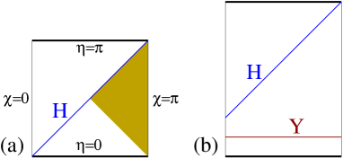
Figure 10: (a) Penrose diagram for empty de Sitter space. $H$ is the future event horizon of an observer on the south pole ($\chi=\pi$). The shaded region is the “southern diamond”. (b) Penrose diagram for a generic solution that asymptotes to de Sitter in the past and future (dS^±). The future event horizon has complete time slices in its past, such as $Y$.

The intersection of both regions forms the “southern diamond”, the region that can be probed by the observer. It is covered by a static coordinate system:

$$ds^{2}=a_{0}^{2}\left[-(1-r^{2})dt^{2}+{dr^{2}\over 1-r^{2}}+r^{2}d\Omega^{2}\right].$$ (122)

Note that the location of event horizons in de Sitter space depends on a choice of observer ($r=0$). Despite this difference, Gibbons and Hawking (1977) showed that the future event horizon of de Sitter space shares many properties with the event horizons of black holes. Classically, objects that fall across the event horizon cannot be recovered. This would seem to endanger the second law of thermodynamics, in the sense discussed in Sec. II.1.3.

Mirroring the reasoning of Sec. II.1.3, one concludes that the horizon must be assigned a semi-classical Bekenstein-Hawking entropy equal to a quarter of its area,

$$S_{\rm dS}=\pi a_{0}^{2}=\frac{3\pi}{\Lambda}.$$ (123)

Gibbons and Hawking (1977) showed that an observer in de Sitter space will detect thermal radiation coming from the horizon, at a temperature $T=1/2\pi a_{0}$.

In pure de Sitter space, there is no matter entropy, so the total entropy is given by Eq. (123).

IX.5.2 dS^± spacetimes

So far we have discussed empty de Sitter space. Generally one is interested in describing a larger class of spacetimes, which might be characterized by asymptotic conditions. Let us consider spacetimes that approach de Sitter space asymptotically both in the past and in the future. We denote this class by dS^±. Its quantum description has recently attracted much attention (e.g., Balasubramanian, Hořava, and Minic, 2001; Strominger, 2001a; Witten, 2001; for extensive lists of references, see, e.g., Balasubramanian, de Boer, and Minic, 2001; Spradlin and Volovich, 2001). Implications of the holographic principle in other accelerating universes have been considered by Hellerman, Kaloper, and Susskind (2001) and Fischler et al. (2001); see also Banks and Dine (2001), Carneiro da Cunha (2002).

If de Sitter space is not completely empty, the Penrose diagram will be deformed. In the asymptotic regions matter is diluted, but in the interior of the spacetime it can have significant density. Gao and Wald (2000) showed under generic assumptions that the back-reaction of matter makes the height of the diagram greater than its width. Then the future event horizon will cross the entire space and converge in the north (Fig. 10b). Because the spacetime approaches empty de Sitter space in the future, the horizon will asymptote to a surface $B$, a sphere of radius $a_{0}$ surrounding the south pole. There will be no matter inside this sphere at late times. All matter will have passed through the future event horizon.

The future event horizon can be regarded as a light-sheet of the surface $B$. This implies that the entropy of all matter on any earlier Cauchy slices cannot exceed a quarter of the area $A(B)=4\pi a_{0}^{2}$. With Eq. (121) we find that

$$S_{\rm global}\leq\frac{3\pi}{\Lambda}.$$ (124)

In particular, this holds for the total entropy in the asymptotic past.

We will not be concerned with the unobservable future region behind the event horizon. We conclude that in a dS^± spacetime, the global entropy cannot exceed ($3\pi$ times) the inverse cosmological constant.

This may seem a surprising result, since the initial equal-time slices can be taken arbitrarily large, and an arbitrary amount of entropy can be placed on them. However, if the matter density becomes larger than the energy density of the cosmological constant during the collapsing phase, the universe will collapse to a big crunch. Then there will be no future infinity, in contradiction to our assumption.

IX.5.3 dS⁺ spacetimes

An even larger class of spacetimes is characterized by the condition that they approach de Sitter space in the asymptotic future. No restrictions are made on the behavior in the past. This class will be labelled dS⁺. In addition to all of the dS^± universes, it includes, for example, flat FRW universes that start with a big bang singularity and are dominated by matter or radiation for some time. At late times, all matter is diluted, only a cosmological constant remains, and the metric approaches that of empty de Sitter space.

Recent astronomical data (Riess et al., 1998; Perlmutter et al., 1999) favor a non-zero value of $\Lambda\sim 10^{-120}$. If this really corresponds to a fixed cosmological constant, our own universe is in the dS⁺ class. This makes the study of de Sitter-like spacetimes, in particular the dS⁺ class of universes, especially significant.

The global entropy at early times is unbounded in this class. In the dS^± class, constraints arise, roughly speaking, because all matter has to “fit” through a throat three-sphere at $\eta=\pi/2$. In the dS⁺ class, there is no need for a contracting phase. The universe can be everywhere expanding, with non-compact spacelike hypersurfaces of infinite total entropy.

However, an observer’s vision is cloaked by the de Sitter event horizon that forms at late times. Let us ask only how much entropy can be detected by any single observer (Banks, 2000a; Fischler, 2000a,b). This is easy to answer because the final entropy is known. At late times, there is no matter and only a de Sitter event horizon, so the total entropy will be given by Eq. (123). By the generalized second law of thermodynamics, the entropy at all other times will be less or equal.

It follows that in a dS⁺ spacetime, the entropy available to any observer cannot exceed ($3\pi$ times) the inverse cosmological constant. The restriction to a single observer is natural in view of black hole complementarity (Sec. III.7).

IX.5.4 Other universes with positive $\Lambda$

Although they comprise a broad class, it still somewhat unnatural to restrict one’s attention to dS⁺ universes. Because of exposure to thermal radiation, an observer in de Sitter space cannot last forever. It is as unphysical to talk about arbitrarily long times as it is to compare the observations of causally disconnected observers.

Moreover, fluctuations in the Gibbons-Hawking radiation cause black holes to form. If they are too big, they can cause a big crunch—a collapse of the entire spacetime. But even the persistent production of ordinary black holes means that any observer who is not otherwise thermalized will fall into a black hole. In short, quantum effects will prevent any observer from reaching ${\cal I}^{+}$.

So how can spacetimes with an absolute entropy bound be usefully characterized? With assumptions involving spherical symmetry, the covariant entropy bound implies that that the observable entropy in any universe with $\Lambda>0$ is bounded by $3\pi/\Lambda$ (Bousso, 2000b). In addition to all dS⁺ spacetimes, this class includes, for example, closed recollapsing FRW universes in which the cosmological constant is subdominant at all times. This result relies on the “causal diamond” definition of an observable region. It would seem to suggest that $\Lambda>0$ may be a sufficient condition for the absolute entropy bound, $S\leq 3\pi/\Lambda$.

At least in $D>4$, however, one can construct product manifolds with fluxes, which admit entropy greater than that of $D$-dimensional de Sitter space with the same cosmological constant (Bousso, DeWolfe, and Myers, 2002). A fully satisfactory classification of spacetimes with finite entropy remains an outstanding problem.

Appendix A General relativity

In this Appendix, we summarize most of the geometric terminology that pervades this paper. No attempts at completeness and precision are made; in particular, we will ignore issues of smoothness. The textbooks of Hawking and Ellis (1973), Misner, Thorne, and Wheeler (1973), and Wald (1984) may be consulted for a more thorough discussion of this material.

Metric, examples, and Einstein’s equation

General relativity describes the world as a classical spacetime ${\cal M}$ with $D-1$ spatial dimensions and one time dimension. Mathematically, ${\cal M}$ is a manifold whose shape is described by a metric $g_{ab}$ of Lorentzian signature $(-,+,\ldots,+)$. In a coordinate system $(x^{0},\ldots,x^{D-1})$, the invariant distance $ds$ between infinitesimally neighboring points is given by

$$ds^{2}=g_{ab}(x^{0},\ldots,x^{D-1})dx^{a}dx^{b}.$$ (125)

Summation over like indices is always implied.

For example, the flat spacetime of special relativity (Minkowski space) in $D=4$ has the metric

$$ds^{2} = -dt^{2}+dx^{2}+dy^{2}+dz^{2}$$ (126)

$$= -dt^{2}+dr^{2}+r^{2}d\Omega^{2}$$ (127)

in Cartesian or spherical coordinates, respectively. A Schwarzschild black hole of mass $M$ is described by the metric

$$ds^{2}=-\left(1-{2M\over r}\right)dt^{2}+\left(1-{2M\over r}\right)^{-1}dr^{2}+r^{2}d\Omega^{2}.$$ (128)

The black hole horizon, $r=2M$, is a regular hypersurface, though this is not explicit in these coordinates. There is a singularity at $r=0$.

Einstein’s equation,

$$G_{ab}=8\pi T_{ab},$$ (129)

relates the shape of space to its matter content. The Einstein tensor, $G_{ab}$, is a nonlinear construct involving the metric and its first and second partial derivatives. The stress tensor, $T_{ab}$, is discussed further below.

Timelike, spacelike, and null curves

A curve is a map from (a portion of) $\mathbb{R}$ into ${\cal M}$. In a coordinate system it is defined by a set of functions $x^{a}(\lambda)$, $\lambda\in\mathbb{R}$. At each point the curve has a tangent vector, ${dx^{a}\over d\lambda}$.

A vector $v^{a}$ pointing up or down in time is called timelike. It has negative norm, $g_{ab}v^{a}v^{b}<0$. Massive particles (such as observers) cannot attain or exceed the speed of light. They follow timelike curves, or worldlines, i.e., their tangent vector is everywhere timelike. A vector $k^{a}$ is called null or light-like if its norm vanishes. light rays follow null curves through spacetime; their tangent vector is everywhere null. Spacelike vectors have positive norm. Spacelike curves connect points that can be regarded as simultaneous (in some coordinate system). No physical object or information follows spacelike curves; this would require superluminal speed.

Geodesic curves

Curves that are “as straight as is possible” in a given curved geometry are called geodesics. They satisfy the geodesic equation,

$${d^{2}x^{a}\over d\lambda^{2}}+\Gamma^{a}_{~{}bc}{dx^{b}\over d\lambda}{dx^{c}\over d\lambda}=\alpha{dx^{a}\over d\lambda}.$$ (130)

(The Christoffel symbols, $\Gamma^{a}_{~{}bc}$, are obtained from the metric and its first derivatives.) Any geodesic can be reparametrized ($\lambda\to\lambda^{\prime}$) so that $\alpha$ vanishes. A parameter with which $\alpha=0$ is called affine.

Unless non-gravitational forces act, a massive particle follows a timelike geodesic. Similarly, light rays don’t just follow any null curve; they generate a null geodesic. We use the terms “light ray” and “null geodesic” interchangeably.

Two points are timelike separated if there exists a timelike curve connecting them. Then they can be regarded as subsequent events on an observer’s worldline. Two points are null separated if they are connected only by a light ray. Two points are spacelike separated if it is impossible for any object or signal to travel from one point from the other, i.e., if they are connected only by spacelike curves.

Visualization and light cones

In all depictions of spacetime geometry in this paper, the time direction goes up, and light rays travel at 45 degrees. The light rays emanating from a given event $P$ (e.g., when a bulb flashes) thus form a cone, the future light cone. light rays arriving at $P$ from the past form the past light cone of $P$. They limit the spacetime regions that an observer at $P$ can send a signal to, or receive a signal from.

Events that are timelike separated from $P$ are in the interior of the light cones. Null separated events are on one of the light cones, and spacelike separated events are outside the light cones. The worldline of a massive particle is always at an angle of less than 45 degrees with the vertical axis. A moment of time can be visualized as a horizontal plane.

Surfaces and hypersurfaces

In this text, the term surface always denotes a $D-2$ dimensional set of points, all of which are spacelike separated from each other. For example, a soap bubble at an instant of time is a surface. Its whole history in time, however, is not a surface.

A hypersurface $H$ is a $D-1$ dimensional subset of the spacetime (with suitable smoothness conditions). $H$ has $D-1$ linearly independent tangent vectors, and one normal vector, at every point. If the normal vector is everywhere timelike (null, spacelike), then $H$ is called a spacelike (null, timelike) hypersurface.

Physically, a spacelike hypersurface can be interpreted as “the world at some instant of time”; hence, it is also called a hypersurface of equal time, or simply, a time slice (Fig. 1). A timelike hypersurface can be interpreted as the history of a surface. A soap bubble, for example, inevitably moves forward in time. Each point on the bubble follows a timelike curve. Together, these curves form a timelike hypersurface.

Null hypersurfaces play a central role in this review, because the holographic principle relates the area of a surface to the number of degrees of freedom on a light-sheet, and light-sheets are null hypersurfaces. If a soap bubble could travel at the speed of light, each point would follow a light ray. Together, the light rays would form a null hypersurface. A particularly simple example of a null hypersurface is a light cone.

More generally, a null hypersurface is generated by the light rays orthogonal to a surface. This is discussed in detail in Sec. V.2. As before, “null” is borderline between “spacelike” and “timelike”. This gives null hypersurfaces great rigidity; under small deformations, they lose their causal character. This is why any surface has only four orthogonal null hypersurfaces, but a continuous set of timelike or spacelike hypersurfaces.

Penrose diagrams

Many spacetimes contain infinite distances in time, or in space, or both. They have four or more dimensions, and they are generally not flat. All of these features make it difficult to draw a spacetime on a piece of paper.

However, often one is less interested in the details of a spacetime’s shape than in global questions. Are there observers that can see the whole spacetime if they wait long enough? Are parts of the spacetime hidden behind horizons, unable to send signals to an asymptotic region (i.e., are there black holes)? Does the spacetime contain singularities, places where Einstein’s equation predicts its own breakdown? If so, are they timelike, so that they can be probed, or spacelike, so that they lie entirely in the past or in the future?

Penrose diagrams are two-dimensional figures that capture certain global features of a geometry while discarding some metric information. The ground rules are those of all spacetime diagrams: time goes up, and light rays travel at 45 degrees. An important new rule is that (almost) every point represents a sphere. This arises as follows.

We assume that the spacetime ${\cal M}$ is at least approximately spherically symmetric. Then the only non-trivial coordinates are radius and time, which facilitates the representation in a planar diagram. Usually there is a vertical edge on one side of the diagram where the radius of spheres goes to zero. This edge is the worldline of the origin of the spherical coordinate system. All other points in the diagram represent $(D-2)$ spheres. (In a closed universe, the spheres shrink to zero size on two opposite poles, and the diagram will have two such edges. There are also universes where the spheres do not shrink to zero anywhere.)

A conformal transformation takes the physical metric, $g_{ab}$, to an unphysical metric, $\tilde{g}_{ab}$:

$$g_{ab}\to\tilde{g}_{ab}=\Omega^{2}g_{ab}.$$ (131)

The conformal factor, $\Omega$, is a function on the spacetime manifold ${\cal M}$. The unphysical metric defines an unphysical spacetime $\tilde{M}$.

A conformal transformation changes distances between points. However, it is easy to check that it preserves causal relations. Two points that are spacelike (null, timelike) separated in the spacetime ${\cal M}$ will have the same relation in the unphysical spacetime $\tilde{\cal M}$.

Penrose diagrams exploit these properties. A Penrose diagram of ${\cal M}$ is really a picture of an unphysical spacetime $\tilde{\cal M}$ obtained by a suitable conformal transformation. The idea is to pick a transformation that will remove inconvenient aspects of the metric. The causal structure is guaranteed to survive. Here are two examples.

A judicious choice of the function $\Omega$ will map asymptotic regions in ${\cal M}$, where distances diverge, to finite regions in $\tilde{\cal M}$. An explicit example is given by Eq. (120). By dropping the overall conformal factor and suppressing the trivial directions along the $(D-2)$ sphere, one obtains the unphysical metric depicted in the Penrose diagram (Fig. 10). The asymptotic infinities of de Sitter space are thus shown to be spacelike. Moreover, the spacetime can now be represented by a finite diagram.

A neighborhood of a singularity in the spacetime ${\cal M}$ can be “blown up” by the conformal factor, thus exposing the causal structure of the singularity. An example is the closed FRW universe, Eq. (73); let us take $w\geq 0$ in Eq. (89) and (88). Again, the prefactor can be removed by a conformal transformation, which shows that the big bang and big crunch singularities are spacelike (Fig. 7).

Conformal transformations yielding Penrose diagrams of other spacetimes are found, e.g., in Hawking and Ellis (1973), and Wald (1984).

Energy conditions

The stress tensor, $T_{ab}$, is assumed to satisfy certain conditions that are deemed physically reasonable. The null energy conditon demands that

$$T_{ab}k^{a}k^{b}\geq 0\mbox{~{}for all null vectors~{}}k^{a}.$$ (132)

This means that light rays are focussed, not anti-focussed, by matter (Sec. VI.1). The causal energy condition is

$$T_{ab}v^{b}T^{ac}v_{c}\leq 0\mbox{~{}for all timelike vectors~{}}v^{a}.$$ (133)

This means that energy cannot flow faster than the speed of light.

In Sec. V.4.1, the null and causal conditions are both demanded to hold for any component of matter, in order to outline a classical, physically acceptable regime of spacetimes in which the covariant entropy bound is expected to hold. The dominant energy condition is somewhat stronger; it combines the causal energy condition, Eq. (133), with the weak energy condition,

$$T_{ab}v^{a}v^{b}\geq 0\mbox{~{}for all timelike vectors~{}}v^{a}.$$ (134)

In cosmology and in many other situations, the stress tensor takes the form of a perfect fluid with energy density $\rho$ and pressure $p$:

$$T_{ab}=\rho u_{a}u_{b}+p(g_{ab}+u_{a}u_{b}),$$ (135)

where the unit timelike vector field $u^{a}$ indicates the direction of flow. In a perfect fluid, the above energy conditions are equivalent to the following conditions on $p$ and $\rho$.

null e. c.: $$\rho\geq-p$$ (136)

causal e. c.: $$|\rho|\geq|p|$$ (137)

null and causal: $$|\rho|\geq|p|\mbox{~{}and}$$ (138)

$$\rho<0\mbox{~{}only if~{}}\rho=-p$$ (139)

weak e. c.: $$\rho\geq-p\mbox{~{}and~{}}\rho\geq 0$$ (140)

dominant e. c.: $$\rho\geq|p|$$ (141)

With the further assumption of a fixed equation of state, $p=w\rho$, conditions on $w$ can be derived.

References

- (1)
- Abdalla and Correa-Borbonet (2001) Abdalla, E., and L. A. Correa-Borbonet, 2001, Aspects of higher order gravity and holography. hep-th/0109129.
- Achucarro and Townsend (1986) Achucarro, A., and P. K. Townsend, 1986, A Chern-Simons action for three-dimensional Anti-de Sitter supergravity theories, Phys. Lett. B180, 89.
- Aharony et al. (2000) Aharony, O., S. S. Gubser, J. Maldacena, H. Ooguri, and Y. Oz, 2000, Large N field theories, string theory and gravity, Phys. Rept. 323, 183. hep-th/9905111.
- Bak and Rey (2000a) Bak, D., and S.-J. Rey, 2000a, Cosmic holography, Class. Quant. Grav. 17, L83. hep-th/9902173.
- Bak and Rey (2000b) Bak, D., and S.-J. Rey, 2000b, Holographic principle and string cosmology, Class. Quant. Grav. 17, L1. hep-th/9811008.
- Balasubramanian and Kraus (1999) Balasubramanian, V., and P. Kraus, 1999, Spacetime and the holographic renormalization group, Phys. Rev. Lett. 83, 3605. hep-th/9903190.
- Balasubramanian et al. (2000) Balasubramanian, V., E. G. Gimon, and D. Minic, 2000, Consistency conditions for holographic duality, JHEP 05, 014. hep-th/0003147.
- Balasubramanian, de Boer and Minic (2001) Balasubramanian, V., J. de Boer, and D. Minic, 2001, Mass, entropy and holography in asymptotically de Sitter spaces. hep-th/0110108.
- Balasubramanian, Hořava and Minic (2001) Balasubramanian, V., P. Hořava, and D. Minic, 2001, Deconstructing de Sitter, JHEP 05, 043. hep-th/0103171.
- Banks (1998) Banks, T., 1998, Matrix theory, Nucl. Phys. Proc. Suppl. 67, 180. hep-th/9710231.
- Banks (1999) Banks, T., 1999, TASI lectures on Matrix theory. hep-th/9911068.
- Banks (2000a) Banks, T., 2000a, Cosmological breaking of supersymmetry or little Lambda goes back to the future II. hep-th/0007146.
- Banks (2000b) Banks, T., 2000b, On isolated vacua and background independence. hep-th/0011255.
- Banks (2000c) Banks, T., 2000c, Supersymmetry and spacetime. Talk given at String Theory at the Millenium, Caltech, Jan. 2000, http://quark.theory.caltech.edu/people/rahmfeld/Banks/ fs1.html.
- Banks and Susskind (1996) Banks, T., and L. Susskind, 1996, The number of states of two dimensional critical string theory, Phys. Rev. D 54, 1677. hep-th/9511193.
- Banks and Dine (2001) Banks, T., and M. Dine, 2001, Dark energy in perturbative string cosmology, JHEP 10, 012. hep-th/0106276.