The Holographic Entropy Bound and Local Quantum Field Theory

Abstract

The maximum entropy that can be stored in a bounded region of space is in dispute: it goes as volume, implies (non-gravitational) microphysics; it goes as the surface area, asserts the “holographic principle.” Here I show how the holographic bound can be derived from elementary flat-spacetime quantum field theory when the total energy of Fock states is constrained gravitationally. This energy constraint makes the Fock space dimension (whose logarithm is the maximum entropy) finite for both Bosons and Fermions. Despite the elementary nature of my analysis, it results in an upper limit on entropy in remarkable agreement with the holographic bound.

PACS numbers: 04.70.-s, 04.62.+v, 04.60.-m, 03.67.-a

An outstanding recent puzzle in gravitational physics is to find a local, microscopic explanation for the ”holographic principle” [1], which asserts that the maximum entropy that can be stored inside a bounded region R in 3-space must be proportional to the surface area $A(\mbox{\script R})$ [as opposed to the volume $V(\mbox{\script R})$] of the region:

$$S_{\max}(\mbox{\script R})=\frac{k_{B}}{4}\frac{A(\mbox{\script R})}{{\l_{p}}^{2}}\;,$$ (1)

where $k_{B}$ is Boltzmann’s constant, and $l_{p}=\sqrt{\mathchar 1406\relax\,G/c^{3}}$ is the Planck length. The most compelling conceptual evidence for the holographic bound comes from black-hole physics and thermodynamics. If there were a physical system enclosed in R whose entropy exceeded $S_{\max}$, it would be possible to violate the second law in the following way: First, one could dump as much energy into R as necessary to bring it to the threshold of gravitational collapse. This process can only increase the entropy contained in R, making it exceed $S_{\max}$ even further. One could then tip the system into full gravitational collapse, leaving nothing but a black hole inside R. The resulting event horizon, being contained in R, necessarily has surface area no larger than $A(\mbox{\script R})$. But according to the Bekenstein formula [2], the entropy of this black hole, given by the right hand side of Eq. (1) with $A(\mbox{\script R})$ replaced by the horizon area, cannot exceed $S_{\max}$. Thus gravitational collapse would appear to cause a sudden decrease in entropy, violating the second law of thermodynamics.

The holographic principle presents a puzzle since derivations based on standard (non-gravitational) micro-physics yield an entropy bound proportional to the volume $V(\mbox{\script R})$ instead of the surface area. To discuss this in the simplest microscopic model, let me choose R to be a standard three-dimensional spacelike cube of size $L$ in Minkowski space, and consider a real, massless (linear) scalar field $\phi$ confined in R. The Fock space is built out of the modes of the field $\phi$, which are the positive frequency solutions of the scalar wave equation $\mathchar 1027\relax\phi=0$ that vanish on $\partial\mbox{\script R}$. These modes are given (up to normalization) by the solutions $\sin(\vec{k}\cdot\vec{x}-\omega_{\vec{k}}\,t)$, where $\omega_{\vec{k}}=c|\vec{k}|$, and the admissible wave vectors $\vec{k}$ are labelled by non-negative integers $m_{x},\;m_{y},\;m_{z}$: $(k_{x},k_{y},k_{z})=(\pi/L)(m_{x},m_{y},m_{z})$. I will often use single-letter labels $i,\;j$ etc. to denote a composite multi-index like $(m_{x},m_{y},m_{z})$. Mode counting and summing various quantities over the modes (and all my computations below will be of this kind) can often be simplified via the standard approximation:

$$\sum_{\vec{k}}\longrightarrow\frac{1}{(\pi/L)^{3}}\int_{P_{+}}d^{3}k\;=\;\frac{1}{c^{3}(\pi/L)^{3}}\frac{4\pi}{8}\int d\omega\,\omega^{2}\;,$$ (2)

where $P_{+}$ denotes the “all-positive” octant of $\vec{k}$-space (consisting of positive $k_{x},\;k_{y},\;k_{z}$), and the last simplification is available whenever the summed quantity depends only on the mode frequency $\omega=c|\vec{k}|$. Consider, for example, the total number of modes, $N$. A natural cutoff at or near the Planck frequency, $\omega=2\pi\mu/\tau_{p}$, makes $N$ finite, where Planck time $\tau_{p}=l_{p}/c$, and $\mu$ is a dimensionless constant of order 1 to be specified by a complete theory of the Planck regime (according to naive Planck-scale physics, $\mu=1$). The total number of modes

$$N=\sum_{i}\,1=\frac{L^{3}}{2\pi^{2}c^{3}}\int_{0}^{2\pi\mu/\tau_{p}}\!\!\omega^{2}\,d\omega=\frac{4\pi\mu^{3}}{3}\left(\frac{L}{l_{p}}\right)^{3}\;$$ (3)

is proportional to the volume $V(\mbox{\script R})=L^{3}$.

The Fock space $\mbox{\script H}_{F}(\mbox{\script R})$ for the theory can be constructed as the Hilbert space spanned by orthonormal basis elements of the form

$$|\Psi\rangle=|n_{1},\;n_{2},\;\cdots\;,\;n_{i},\;\cdots\;,n_{N}\rangle\;\;,\;\;\;\;\;\;n_{j}\in\mbox{\bbold N}\;$$ (4)

which denotes a state with $n_{i}$ particles occupying mode $i$. With Fermi statistics, each $n_{i}$ is restricted to the values $n_{i}=0,\;1$, while with Bose statistics the $n_{i}$ can be arbitrarily large integers. The entropy associated to any quantum state of the field is given by $S=-k_{B}{\rm Tr}(\rho\log\rho)$, where $\rho$ is the density matrix of the state. The state with the largest possible entropy is the maximally mixed

$$\rho_{\max}=\frac{1}{\dim\mbox{\script H}_{F}(\mbox{\script R})}\;\mbox{\bf 1}\;,$$ (5)

the identity operator normalized by the dimension of the Fock space $\mbox{\script H}_{F}(\mbox{\script R})$. It follows that maximum entropy is proportional to the log-dimension of $\mbox{\script H}_{F}(\mbox{\script R})$:

$$S_{\max}=-k_{B}{\rm Tr}(\rho_{\max}\log\rho_{\max})=k_{B}\log\dim\mbox{\script H}_{F}(\mbox{\script R})\;.$$ (6)

The Fock-space dimension (and hence the maximum entropy) is infinite for Bosons unless the number of particles in each mode $i$ is constrained by a finite bound. Assuming that the $n_{i}$ are so constrained,

$$n_{i}<D\;,\;\;\;\;\;\;\forall i$$ (7)

for some fixed integer $D$, the number of states of the form Eq. (4) is $D^{N}$ [$=\dim\mbox{\script H}_{F}(\mbox{\script R})\;$], and Eqs. (6) and (3) give

$$S_{\max}=k_{B}(\log D)\,N=\frac{4\pi\mu^{3}\log D}{3}k_{B}\frac{V(\mbox{\script R})}{l_{p}^{3}}\;.$$ (8)

For Fermions (the case $D=2$), the maximum entropy is proportional to volume. For Bosons, we must conclude either that the entropy is unbounded, or we must regularize it with the occupation-number constraints Eq. (7) in which case the bound is again proportional to volume. Even if the constraints $D$ were allowed to depend on the mode frequency $\omega_{i},\;$ setting $D_{0}\equiv\min\{D_{i}\}$ ($D_{0}\mathchar 13374\relax 2$) it is clear that $\dim{\mbox{\script H}_{F}}(\mbox{\script R})\mathchar 13374\relax{D_{0}}^{N}$, and Eqs. (6) and (3) imply

$$S_{\max}\mathchar 13374\relax\frac{4\pi\mu^{3}\log D_{0}}{3}k_{B}\frac{V(\mbox{\script R})}{l_{p}^{3}}\;,$$ (9)

still in violent disagreement with the holographic bound Eq. (1).

I will now introduce an ansatz, which consists of imposing an upper bound on the total energy of states (so that the states are stable against collapse in semiclassical gravity), and proceed to show that the resulting constrained Fock space has the right dimension consistent with the holographic principle. Before proceeding to this calculation and a discussion of the consequences of the ansatz, a few comments on the general validity of the holographic bound, and why I will defer dealing with its generalizations: It has been noted by many authors [3, 4, 5] that the bound Eq. (1) cannot possibly hold for arbitrary spacelike 3-volumes R. Even in flat, Minkowski spacetime, it is not difficult to find examples of R for which the bound as given by Eq. (1) is violated. In these examples, the region R is contained in a curved spacelike hypersurface instead of a flat $\{t={\rm const.}\}$ slice of Minkowski spacetime, making different parts of its boundary $\partial\mbox{\script R}$ Lorentz boosted at different speeds, and making its surface area arbitrarily small. It is clear that the thermodynamic argument following Eq. (1) above breaks down for such volumes (the area of the black hole after collapse can exceed the surface area of $\partial\mbox{\script R}$). A covariant generalization of the holographic bound[4, 3], which replaces the entropy content of the volume R with the entropy contained on the ingoing null congruence emanating from $\partial\mbox{\script R}$, appears to have more general validity[5]. While the microscopic derivation of the holographic bound I present below is likely to prevail more generally for Minkowski ($\{t={\rm const.}\}$) volumes with sufficiently “regular” boundary [6], the more interesting question of how the derivation is relevant to the covariant holographic principle will be discussed in a forthcoming paper [7].

Neglecting the small Casimir-effect contribution to the vacuum stress-energy, the regularized total Hamiltonian for the scalar field $\phi$ can be written in the form $H=\int_{\mbox{\script R}}:\!T_{00}\!:\,d^{3}x=\sum_{i}\mathchar 1406\relax\omega_{i}{a_{i}}^{\dagger}a_{i}$, where ${a_{i}}^{\dagger},\;a_{i}$ are the usual creation and annihilation operators for the mode $i$. The total energy of a Fock state of the form Eq. (4) is

$$\langle\Psi|H|\Psi\rangle=\langle\Psi|\sum_{i}\mathchar 1406\relax\omega_{i}{a_{i}}^{\dagger}a_{i}|\Psi\rangle=\sum_{i}\mathchar 1406\relax\omega_{i}n_{i}\;.$$ (10)

Let me now introduce the ansatz that the Hilbert space of the theory contains only those Fock states $|\Psi\rangle$ for which

$$\langle\Psi|H|\Psi\rangle=\sum_{i}\mathchar 1406\relax\omega_{i}n_{i}\;<\;E_{\max}\;,$$ (11)

where $E_{\max}\sim(c^{4}/G)L$ is an upper bound on energy which ensures that the field $\phi$ is in a stable configuration against gravitational collapse according to semiclassical Einstein equations. More precisely: the Fock space $\mbox{\script H}_{F}(\mbox{\script R})$ of the theory consists of the linear span of the (finitely many) states of the form Eq. (4) satisfying the constraint Eq. (11). It is important to note that this ansatz is consistent with the linear structure of Fock space; any $|\Psi\rangle\in\mbox{\script H}_{F}(\mbox{\script R})$ obeys the same energy bound: $\langle\Psi|H|\Psi\rangle<E_{\max}$. For if $|\Psi\rangle$ can be written as a linear combination $|\Psi\rangle=\sum_{\alpha}c_{\alpha}|{\Psi}_{\alpha}\rangle$, $\sum_{\alpha}|c_{\alpha}|^{2}=1$, of the basis states $|{\Psi}_{\alpha}\rangle$ satisfying Eq. (11), then, since $|{\Psi}_{\alpha}\rangle$ are eigenstates of the Hamiltonian $H$,

$\displaystyle\langle\Psi|H|\Psi\rangle=\sum_{\alpha}|c_{\alpha}|^{2}\langle{\Psi}_{\alpha}|H|{\Psi}_{\alpha}\rangle<\sum_{\alpha}|c_{\alpha}|^{2}E_{\max}=E_{\max}\;.$

Introducing the dimensionless frequencies $\Omega_{i}$ and the dimensionless energy bound $B$ via

$$\Omega_{i}\equiv\tau_{p}\,\omega_{i}\;,\;\;\;\;\;\;B\equiv\frac{\tau_{p}}{\mathchar 1406\relax}\,E_{\max}\;,$$ (12)

the ansatz Eq. (11) can be rewritten in the form

$$\sum_{i}n_{i}\,\Omega_{i}\;<\;B\;.$$ (13)

The precise value of $B$ will depend on the details of a self-consistent semiclassical (or fully quantum) theory of gravity; nevertheless, I will assume that it does not differ much from the value predicted by the hoop conjecture [8] applied to the cube R:

$$B=\eta\,\frac{\sqrt{3}}{4}\;\frac{L}{l_{p}}\;,$$ (14)

where $\eta$ is a dimensionless number of order 1. According to the classical hoop conjecture, $\eta=1$.

What is the dimension of the Fock space constrained as in Eq. (11)? For both Bosons and Fermions, the dimension is equal to the combinatorial quantity

$$\dim\mbox{\script H}_{F}(\mbox{\script R}) = W(B)\equiv\mbox{\# of}\;(n_{1},\;n_{2},\;\cdots\;,\;n_{N}),$$ (16)

$$\;n_{i}\in\mbox{\bbold N},\;\mbox{such that}\;\sum_{i}n_{i}\Omega_{i}<B\;,$$

the cardinality of the space of solutions to Eq. (13) in non-negative integer $N$-tuples. With Fermi statistics, the $n_{i}$ are further constrained by $n_{i}\in\{0,1\}$; for Bosons, there are no additional constraints. The computation of $S_{\max}$ now reduces to knowing how to count the quantity $W(B)$.

First the computation for Bosons, since Bose statistics clearly leads to the larger dimension: Notice that the inequality Eq. (13) can be written in the form

$$\vec{n}\cdot\vec{\Omega}<B\;,$$ (17)

where the vectors $\vec{n}=(n_{1},\cdots,n_{N})$ and $\vec{\Omega}=(\Omega_{1},\cdots,\Omega_{N})$ live in $N$-dimensional Euclidean space ${\mbox{\bbold R}}^{N}$. Geometrically, the quantity $W(B)$ is the number of points of the integer lattice ${\mbox{\bbold Z}}^{N}$ which are contained in the convex subset ${\cal P}^{N}\equiv\{\vec{x}\cdot\vec{\Omega}<B,\;x_{i}\mathchar 13374\relax 0\}$ of ${\mbox{\bbold R}}^{N}$. ${\cal P}^{N}$ is a polyhedral volume in the positive $2^{N}$’th sector ($x_{i}\mathchar 13374\relax 0$) of ${\mbox{\bbold R}}^{N}$, bounded by the hyperplane $\{\vec{x}\cdot\vec{\Omega}=B\}$ (see Fig. 1 for the geometry of ${\cal P}^{N}$ for $N=3$). At first thought, one might be tempted to conclude that $W(B)$ is simply proportional to the volume of ${\cal P}^{N}$, since each unit cell of the integer lattice $\mbox{\bbold Z}^{N}$ contains on average 1 lattice points and has unit volume. It is easy to show that the volume of a polyhedron ${\cal P}^{n}$ in $\mbox{\bbold R}^{n}$ whose vertices (the points where its bounding hyperplane intersects the coordinate axes) are located at $x_{i}=l_{i},\;i=1,2,\cdots,n$, is

$$V({\cal P}^{n})=\frac{1}{n!}\;l_{1}\,l_{2}\,\cdots\,l_{n}\;.$$ (18)

For ${\cal P}^{N}=\{\vec{x}\cdot\vec{\Omega}<B,\;x_{i}\mathchar 13374\relax 0\}$, these edge lengths $l_{i}$ are

$$l_{i}=\frac{B}{\Omega_{i}}\;.$$ (19)

Using $\prod_{i}(B/{\Omega_{i}})=\exp\sum_{i}\log(B/\Omega_{i})$, $V({\cal P}^{N})$ can be calculated with the help of Eq. (2); asymptotically ($L\gg l_{p}$),

$$V({\cal P}^{N})\sim\frac{1}{N!}\exp\left[\frac{4\pi\mu^{3}}{3}\left(\frac{L}{l_{p}}\right)^{3}\log B\right]\;.$$ (20)

According to Eqs. (14) and (3) and Stirling’s formula $\log N!\sim N\log N-N$, $V({\cal P}^{N})$ vanishes exponentially: $V({\cal P}^{N})\sim\exp[-N\log(N/B)]$ for large $L/l_{p}\;$; ${\cal P}^{N}$ does not even contain a single lattice point of $\mbox{\bbold Z}^{N}$ in its interior!   Solutions of Eq. (13) are distributed skin-deep on the polyhedron ${\cal P}^{N}$; the bulk of the contribution to $W(B)$ comes from points on the boundary of ${\cal P}^{N}$ (Fig. 1). This boundary is comprised of $N$ polyhedra ${\cal P}^{N-1}$ of dimension $N-1$,   each of which in turn have boundaries made

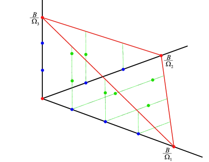
FIG. 1.: Example geometry of ${\cal P}^{3}$, with $\lfloor B/\Omega_{1}\rfloor=4$, $\lfloor B/\Omega_{2}\rfloor=\lfloor B/\Omega_{3}\rfloor=3$. The boundary of ${\cal P}^{3}$ consists of three ${\cal P}^{2}$ polyhedra (the right-triangular walls), three edges (${\cal P}^{1}$’s), and four vertices. Contributing to $W(B)$ are 7 points on the ${\cal P}^{2}$ walls (green dots), 7 points on the edges (blue dots), and four vertices (red dots). There is only one contributing interior point (not shown); it is located at $n_{1}=n_{2}=n_{3}=1$.

up of $N-1$ $\;\,{\cal P}^{N-2}$’s, and so on. By iterating the reasoning above inductively to the lower-dimensional components of this scaffolding which comprises ${\cal P}^{N}$’s boundary, it is not difficult to show that $W(B)$ can be evaluated as

$$W(B)=1+N+\sum_{n=1}^{N}\frac{1}{n!}S_{n}\;,$$ (21)

where, for $1\mathchar 13366\relax n\mathchar 13366\relax N$,

$$S_{n}\equiv\sum_{i_{1}<i_{2}<\cdots<i_{n}}(l_{i_{1}}-1)(l_{i_{2}}-1)\cdots(l_{i_{n}}-1)\;.$$ (22)

Here I made use of Eq. (17) to compute the interior volume of each sub-polyhedron ${\cal P}^{n}$ on the boundary. The edge lengths $l_{i_{k}}$ are reduced by 1 so that only interior points of ${\cal P}^{n}$ contribute to $W(B)$, and overcounting of points that lie on the boundaries of each ${\cal P}^{n}$ is avoided.

Each sum $S_{n}$ contains $N\choose n$ summands, resulting in $2^{N}$ terms in Eq. (20). How can Eq. (20) be evaluated? The first key observation is a sequence of elementary algebraic identities which leads to a recursion relation for $S_{n}$. If I set $S_{0}\equiv 1$, and introduce the quantities

$$P_{m}\equiv\sum_{i=1}^{N}(l_{i}-1)^{m}\;,\;\;\;\;\;\;1\mathchar 13366\relax m\mathchar 13366\relax N\;,$$ (23)

then this sequence of algebraic identities are

$$S_{0} = 1\;,$$ (24)

$$S_{1} = P_{1}\;,$$ (25)

$$S_{2} = \frac{1}{2}(P_{1}S_{1}-P_{2})\;,$$ (26)

$$S_{3} = \frac{1}{3}(P_{1}S_{2}-P_{2}S_{1}+P_{3})\;,$$ (27)

$$\vdots \vdots$$ (28)

leading to the recursion formula

$$S_{m}=\frac{1}{m}\sum_{j=1}^{m}(-1)^{j-1}P_{j}\,S_{m-j}\;,\;\;\;\;1\mathchar 13366\relax m\mathchar 13366\relax N\;.$$ (29)

The next key observation is that in the regime $L/l_{p}\gg 1$,

$$(P_{1})^{m}\gg P_{m}\;,\;\;\;\;\;\;\forall\;m=2,\;\cdots\;,\;N\;.$$ (30)

The proof consists of a straightforward evaluation of the sums $P_{m}$ via the integral formula Eq. (2), which gives

$$P_{1} = \frac{L^{3}}{2\pi^{2}c^{3}}\int_{0}^{2\pi\mu/\tau_{p}}\omega^{2}\left(\frac{B}{\tau_{p}\omega}-1\right)\,d\omega$$ (31)

$$= \mu^{2}\left(\frac{L}{l_{p}}\right)^{3}B-N=\mu^{2}\left(\frac{L}{l_{p}}\right)^{3}B\left(1-\frac{4\pi\mu}{3B}\right)\;.$$ (32)

While for higher $m$ (since lowest $\omega$ is $\pi c/L$, no true infrared divergences occur at $\omega=0$), e.g., for $m\mathchar 13374\relax 4$,

$$P_{m}\sim\frac{4\pi}{m-3}\left(\frac{BL}{\pi l_{p}}\right)^{m}\;.$$ (33)

Comparison of Eq. (26) with Eq. (27) should make Eq. (25) obvious (see [7] for full details). It follows that in the recursion formula Eq. (24), the first term of the sum dominates over all others, proving that asymptotically

$$S_{m}\sim\frac{1}{m!}\;{P_{1}}^{m}\;,$$ (34)

and, by Eq. (20) and the asymptotic behavior Eq. (19),

$$W(B)=N+q(P_{1})\;,\;\;\mbox{where}\;\;q(z)\equiv\sum_{n=0}^{\infty}\frac{z^{n}}{(n!)^{2}}\;.$$ (35)

To discover the entire analytic function $q(z)$, notice that it satisfies the differential equation $q_{,zz}+q_{,z}/z-q/z=0$, whose solutions are Bessel functions of $\sqrt{z}$. Indeed, $q(z)=I_{0}(2\sqrt{z})$, the zeroth-order Bessel function of the second kind [9], with asymptotic behavior as $|z|\rightarrow\infty$:

$$I_{0}(z)\sim\frac{e^{z}}{\sqrt{2\pi z}}\left[1+\frac{1}{8\,z}+O\left(\frac{1}{z^{2}}\right)\right]\;.$$ (36)

Finally, combining Eqs. (29) and (26),

$$W(B)=N+I_{0}\left[2\mu\left(\frac{B\,L^{3}}{{l_{p}}^{3}}\right)^{1/2}\right]\;,$$ (37)

and Eqs. (14) and (30) give, asymptotically,

$$S_{\max}=k_{B}\log W(B)=k_{B}\,3^{1/4}\,\mu\sqrt{\eta}\,\left(\frac{L}{l_{p}}\right)^{2}\;,$$ (38)

which [10] is in full agreement with the holographic bound Eq. (1) if $\;\mu\sqrt{\eta}\,=\,3^{3/4}/2\,\cong\,1.14$ [note: $A(\mbox{\script R})=6L^{2}$].

With Fermi statistics, the computation of $W(B)$ involves a different but more straightforward approach, relying on a probabilistic analysis of the distribution of energy over the $2^{N}$ subsets (which label the Fermionic states) of the set of all modes. The result is:

$$S_{\max}=k_{B}\,\frac{2}{3\pi\mu}\,B\,\left[1+\log\left(\frac{3\pi\mu}{2}\frac{N}{B}\right)\right]\;,$$ (39)

i.e., $S_{\max}$ is proportional to $(L/l_{p})\log(L/l_{p})$. The full derivation and a discussion of the physical significance of Eq. (33) will be given in [7].

The ansatz Eq. (11) does lead to the correct holographic entropy bound, but how seriously should it be taken? Here are some of the possible consequences of taking Eq. (11) dead seriously as a fundamental physical law:

The commutation relations (CCR) for Bose statistics

$$[\,a_{i}\,,\,{a_{j}}^{\dagger}\,]=\delta_{ij}\,\mbox{\bf 1}$$ (40)

are incompatible with a finite-dimensional Fock space, as can be readily seen by taking the trace of both sides of Eq. (34) [the result is: $0=\delta_{ij}\dim\mbox{\script H}_{F}(\mbox{\script R})$]. Indeed, according to the ansatz Eq. (13), whether they obey the Bose CCR or the Fermi CAR, the operators ${a_{i}}^{\dagger}$ must satisfy the algebraic relations

$$\prod_{i=1}^{N}({a_{i}}^{\dagger})^{n_{i}}=0\;\;\;\mbox{whenever}\;\;\;\sum_{i=1}^{N}n_{i}\,\Omega_{i}\mathchar 13374\relax B\;,$$ (41)

which imply an algebraic structure drastically different from the CCR (or CAR). One possible way to specify the new algebra (for Bosons) is to impose Eq. (35) along with

$$[\,a_{i}\,,\,{a_{j}}^{\dagger}\,]=\delta_{ij}\,\mbox{\bf 1}+C_{ij}\;,$$ (42)

where $C_{ij}$ are operators which satisfy

$${\rm Tr}\,C_{ij}=-\delta_{ij}\,\dim\mbox{\script H}_{F}(\mbox{\script R})=-\delta_{ij}\,W(B)\;$$ (43)

and whose matrix elements $\langle\Psi|C_{ij}|\Psi^{\prime}\rangle\approx 0$ for low-energy states $|\Psi\rangle$, $|\Psi^{\prime}\rangle$. How can this construction be carried out uniquely, and what are the consequences of the new algebra for physically observable quantities such as expectation values of the stress-energy tensor?

An immediate consequence of Eqs. (35) and (36) is the breakdown of Lorentz invariance at scales much earlier than Planck; namely at a new temperature scale

$$k_{B}T_{c}\sim\frac{\mathchar 1406\relax c}{\sqrt{L\,l_{p}}}\;\;.$$ (44)

For a region R of size $\sim\!\!L$, $T_{c}$ is that temperature at which massless Bosons confined in R have sufficient thermal energy for gravitational collapse [11]. Relative to the characteristic temperature $k_{B}T\!\!\sim\!\!\mathchar 1406\relax c/L$, $\;T_{c}$ corresponds to Lorentz boosts (blueshifts) of order $\gamma\!\!\sim\!\!z\!\!\sim\!\!\sqrt{L/l_{p}}$, whereas the Planck temperature ($k_{B}T_{p}\!\!\sim\!\!\mathchar 1406\relax c/l_{p}$) corresponds to (much larger) boosts of order $\gamma\!\!\sim\!\!z\!\!\sim\!\!L/l_{p}$. For feature sizes $L$ at the sub-nucleon scales, the temperature Eq. (38) is reachable via Lorentz boosts that lie only a few orders of magnitude beyond those envisioned in the large hadron colliders currently under construction [12].

- [1] L. Susskind, J. Math. Phys. 36, 6377 (1995).
- [2] J. D. Bekenstein, Phys. Rev. D 7, 2333 (1973).
- [3] R. Bousso, Rev. Mod. Phys. 74, 825 (2002).
- [4] R. Bousso, Class. Quantum Grav. 17, 997 (2000).
- [5] E. E. Flanagan, D. Marolf, and R. M. Wald, Phys. Rev. D 62, 084035 (2000).
- [6] Since the highest-frequency modes make the largest contribution to the entropy, it appears plausible that the present derivation of the holographic bound is insensitive to the detailed geometry of the boundary as long as the average radius of curvature of is much larger than . See [7] for the calculation with a spherical region R, and for an analysis of the more general case.
- [7] U. Yurtsever, in preparation.
- [8] K. S. Thorne, in Magic without Magic: John Archibald Wheeler, ed. J. Klauder (Freeman, San Francisco, 1972).
- [9] M. Abramowitz and I. A. Stegun, Handbook of Mathematical Functions (Dover, New York, 1973).
- [10] The result Eq. (32) was derived for a Bosonic massless spin-0 field. For higher-spin massless Bosons with two polarization degrees of freedom (e.g. photons), the calculation is exactly the same [7] except the number of modes is doubled along with the quantity , and is larger by a factor of . Precise agreement with the holographic bound Eq. (1) then requires .
- [11] It is interesting to note that statistical thermodynamics, in which entropy (Bose or Fermi), gives the “wrong answer” for . See [7] for a full discussion.
- [12] S. Dimopoulos and G. Landsberg, Phys. Rev. Lett. 87, 161602 (2001); S. B. Giddings and S. Thomas, http://xxx.lanl.gov/abs/hep-th/0106219.