Extended open inflationary universes

Abstract

In this paper we study a type of one-field model for open inflationary universe models in the context of the Jordan-Brans-Dicke theory. In the scenario of a one-bubble universe model we determine and characterize the existence of the Coleman-De Lucia instanton, together with the period of inflation after tunnelling has occurred. Our results are analogous to those found in the Einstein General Relativity models.

I Introduction

Until recently, inflation AG ; AAPS ; AL was always associated with a flat universe, due to its ability to drive the spatial curvature to zero so effectively. In fact, requiring sufficient inflation to homogenize random initial conditions drives the universe very close to critical density. However, current observations, e.g. the cosmic microwave background (CMB) radiation, show a large degree of homogeneity, but are as yet inconclusive as to spatial curvature. Because of this, some authors have put forward the idea of considering other models in which the curvature does not vanished.

In the context of an open scenario, it is assumed that the universe has a lower-than-critical matter density and, therefore, a negative spatial curvature. Several authors re3 ; re4 ; re5 ; re6 , following previous speculative ideas re1 ; re2 , have proposed possible scenarios in which open universes may be realized, and its consequences, such that density perturbations, have been explored UMRS . Very recently the possibility has been considered to create an open universe from the perspective of the brane-world scenarios MBPGD .

The need to consider open models is reflected in the fact that primordial perturbations and their corresponding power spectrum give rise in a natural way not only to adiabatic perturbation but also to isocurvature perturbations. This generic situation is obtained, for instance, in the case where two fields are excited during inflation. We expect this sort of situation in a model in which the inflaton $\sigma$ and the Jordan-Brans-Dicke (JBD) $\phi$ scalar fields are present KEHKSJV .

The basic idea in an open universe is that a symmetric bubble nucleates in the de Sitter space background, and its interior undergoes a stage of slow-roll inflation, where the parameter $\Omega_{0}$ can be adjusted to any value in the range $0<\Omega_{0}<1$.

Bubble formation in the false vacuum is described by the Coleman-De Lucia(CDL) instantons re7 . Once a bubble has taken place by this mechanism, the bubble’s inside looks like an infinite open universe. The problem with this sort of scenario is that the instanton exists only if the following inequality $\mid V^{{}^{\prime\prime}}\mid>H^{2}$ is satisfied during the tunneling process. On the contrary, during inflation the inequality $\mid V^{{}^{\prime\prime}}\mid\ll H^{2}$ is satisfied (slow-roll approximation). From now on $V^{{}^{\prime\prime}}$ stands for $d^{2}V/d\sigma^{2}$, where $\sigma$ is the inflaton scalar field and $V=V(\sigma)$, the inflaton potential. Linde solves this problem by proposing a simple one-field model in Einstein’s general relativity (GR) theory re6 (see also ref. re8 ). At this point, we should mention that Ratra and Peebles were the first to elaborate on the open inflation model RaPe .

In ref. re9 a one-field model for open inflation by using scalar-tensor type of theory (a nonminimally coupled scalar field with polynomial potentials)is studied. Here, the scalar potential associated with the JBD field is assumed to be $\displaystyle V(\phi)=\frac{1}{2}m^{2}\phi^{2}(1+f^{2}(\phi))$. Then, the arbitrary function $f(\phi)$ is fixed in such a way that in the Einstein frame the resulting effective action coincides with the one used by Linde re6 . This certainly restricts not only the evolution of the JBD field but also the parameters that enter into the model.

The purpose of the present paper is to study a one-field open inflation in a JBD theory re10 , where the inflaton field $\sigma$ is of the same nature as that described by Linde re6 . In this sense, our model will be a genuine, extended open inflationary universe model.

The plan of the paper is as follows: In Sec. II we numerically write and solve the field equations in a Euclidean spacetime. Here, the existence of the CDL instanton for two different models are described. In Sec. III we determine the characteristic of the open inflationary universe model that is produced after tunnelling has occurred. In Sec. IV we determine the corresponding density perturbations for our models. Our results are compared with the analogous results obtained by using the Einstein theory of gravity. Finally, we conclude in Sec. V.

II The Euclidean cosmological equations in JBD theory

We consider the effective action given by

$$S\,=\,\int{d^{4}x\,\sqrt{-g}}\,\left[\,\frac{1}{2}\,\varepsilon\,\phi^{2}\,R\,-\,\frac{1}{2}\,\partial_{\mu}\phi\,\partial^{\mu}\phi-{\cal{L}}(\sigma)\right],$$ (1)

where

$${\cal{L}}(\sigma)\,=\,\frac{1}{2}\partial_{\mu}\sigma\partial^{\mu}\sigma\,+\,V(\sigma),$$

and $R$ is the Ricci scalar curvature, $\phi$ is the JBD scalar field, and $\varepsilon$ is a dimensionless coupling constant that, in terms of JBD parameter $\omega$, is equivalent to $1/4\,\varepsilon$. $V(\sigma)$is an effective scalar potential associated with the inflaton field, $\sigma$.

The $O(4)$- invariant Euclidean spacetime metric is described as

$$d{s}^{2}\,=\,d{\tau}^{2}\,+\,a(\tau)^{2}\,(\,\,d{\psi}^{2}\,+\,\sin^{2}\psi\,d{\Omega^{2}_{2}}\,\,),$$ (2)

where $a(\tau)$ is the scale factor, and $\tau$ represents the Euclidean time.

When metric (2) is introduced into action (1), we obtain the following field equations:

$$\left(\frac{a^{,}}{a}\right)^{2}+2\frac{a^{,}}{a}\frac{\phi^{,}}{\phi}=\frac{1}{a^{2}}+\frac{1}{3\varepsilon\phi^{2}}\left[\frac{\phi^{,\,2}}{2}+\frac{\sigma^{,\,2}}{2}-V(\sigma)\right]\,,$$ (3)

$$\phi^{,,}+3\frac{a^{,}}{a}\phi^{,}+\frac{\phi^{,\,2}}{\phi}+\frac{1}{1+6\varepsilon}\left[\frac{\sigma^{,\,2}}{\phi}+\frac{4}{\phi}V(\sigma)\right]=0\,\,,$$ (4)

$$\sigma^{,,}\,=\,-3\,\frac{a^{,}}{a}\,\sigma^{,}\,+\,\frac{dV}{d\sigma}\,\,,$$ (5)

where the primes denote derivatives with respect to $\tau$. From now on we will use units where c = $\hslash$=M_p=G^-1/2 = 1.

From Equations (3), (4) and (5) we obtain

$$a^{,,}=2\frac{a^{,}\phi^{,}}{a\phi}-\frac{a}{3\varepsilon\phi^{2}}\left[\phi^{,2}+\frac{1+3\varepsilon}{1+6\varepsilon}\sigma^{,\,2}+\frac{1-6\varepsilon}{1+6\varepsilon}V(\sigma)\right].$$ (6)

The first model considered corresponds to the effective potential used by Lindere6 :

$$V(\sigma)\,=\,\frac{m^{2}\,\sigma^{2}}{2}\left(\,1\,+\,\frac{\alpha^{2}}{\beta^{2}+(\sigma-v)^{2}}\right)\,,$$ (7)

where $\alpha$, $\beta$ and $v$ are arbitrary constants. In this potential the first term controls inflation after quantum tunneling has occurred. Its form coincides with that used in the simplest chaotic inflationary universe model, $m^{2}\sigma{{}^{2}}/2$. The second term controls the bubble nucleation, whose role is to create an appropriate shape in the inflaton potential, $V(\sigma)$, where its maximum occurs near $\sigma$ = $v$. Following Lindere6 we take $\beta^{2}$=2$\alpha^{2}$, $\beta$=0.1 $v$=3.5 and $m$= 1.5 $\times$10^-6. Certainly, this is not the only choice, since other values for these parameters can also lead to a successful open inflation scenario (with any value of $\Omega$, from 0 and 1).

We have solved the field Equations (3)-(5) numerically. The boundary conditions that we used are those in which $\phi^{,}$=$\sigma^{,}$=0 and $a^{,}=1$ at $a=0$, for various values of the JBD parameter, $\omega$. At $\tau\approx 0$, the scalar field $\sigma=\sigma_{T}$ lies in the ”true vacuum”, near the maximum of the potential, $V(\sigma)$, and at $\tau\neq 0$, the same field is found closed to the false vacuum, but now with a different value, $\sigma=\sigma_{F}$. In our model, when the scalar field $\sigma$ evolves from some initial value $\sigma_{F}\cong\sigma_{i}\approx 3.6$ to the final value $\sigma_{T}\cong\sigma_{f}\approx 3.4$, we found that the CDL instanton does exist, and the extended open inflationary universe scenario can be realized. Figure 1 shows how the scale factor evolves during the tunneling process.

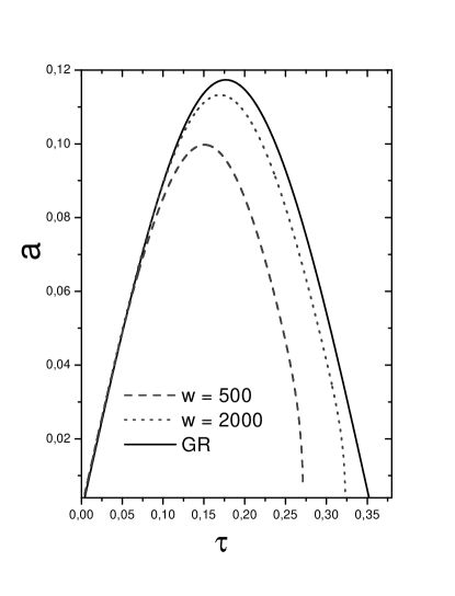
Figure 1: For our model we plot the scale factor a($\tau$) as a function of the Euclidean time $\tau$, for two different values of the JBD parameter, $\omega$=500 and $\omega$= 2000. GR represents the same graph, but it was obtained by using the Einstein GR theory. We have assumed constant $m$ to be equal to one.

Note that the interval of tunneling, specified by $\tau$, decreases when the parameter $\omega$ decreases, but its shapes remain practically similar. The evolution of the inflaton field as a function of the Euclidean time is shown in Fig. 2. Note the similar quantities that $\sigma(\tau)$ contracts at the beginning of the inflationary era ($\tau=0$).

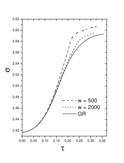
Figure 2: The instanton $\sigma(\tau)$ as a function of the Euclidean time $\tau$ is shown for Einstein’s GR and JBD theories. In the latter case we have assumed $\omega=500$ and $\omega=2000$. As before, we have assumed $m=1$.

In Fig. 3 we show $|V^{{}^{\prime\prime}}|\,/\,H^{2}$ as a function of the Euclidean time $\tau$ for our model. From this plot we observe that, most of the time during the tunneling, we obtain $|V^{{}^{\prime\prime}}|\,>\,H^{2}$, analogous to what occurs in the Einstein’s GR theory. Note that, as far as we decrease the value of the parameter $\omega$, the peak becomes narrower and deeper, and thus the above inequality is better satisfied.

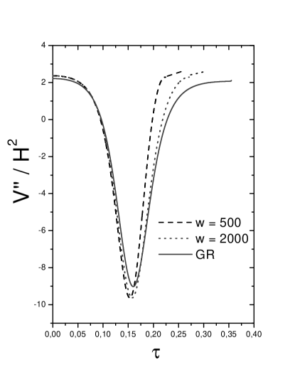
Figure 3: This plot shows how during the tunneling process the inequality $|V^{{}^{\prime\prime}}|\gg H^{2}$ is satisfied for two values of $\omega$($\omega$=500 and $\omega$=2000 for JBD theory). The continuous line represents the same inequality for Einstein’s GR theory. Again, we have taken $m=1$.

In our model, it is possible to numerically show that the CDL instanton $\sigma(\tau)$ exists, and for various values of the $\omega$ parameter, it presents a similar behavior to that described in the Linde’s paper re6 . The values actually coincide for small $\tau$, and its values (after tunneling has occurred) coincide in the two theories, i.e. Einstein’s GR and JBD theories. This result shows that the value that $\sigma$ obtains at the end of the tunneling process is independent of the $\omega$ parameter. On the other hand, the numerical solution shows that the evolution of the JBD field $\phi$ during the tunneling process is such that it remains practically constant for $\tau\leq 0.3$, and it then decreases for $\tau>0.3$.

At this point, we would like to consider a new effective potential:

$$V(\sigma)\,=\,\frac{m^{2}\,\sigma^{2}}{2}\left(\,1\,+\,\frac{\alpha^{2}\,tanh(v-\sigma)}{\beta^{2}+(\sigma-v)^{2}}\right)\,.$$ (8)

which is quite similar to that studied in Reference re8 . Here $\alpha$, $\beta$ and $v$ are arbitrary constants. For completeness, we will restrict ourselves to the particular case in which the different constants take the values m = 1.5 $\times$ 10^-6, $v$ = 3.5, $\alpha^{2}$ = 0.1, and $\beta^{2}$ = 0.01. The shape of this potential is shown in Fig. 4. We should mention that both effective potentials (7) and (8) present a pronounced peak, which is necessary for open inflation to occur. The nature of these potentials may be varied. For instance, present-day supersymmetry and supergravity theories include many scalar fields, whose interaction potentials may be arbitrary to certain extent. It is therefore useful to study the de Sitter stage which is produced by effective potentials, such as those expressed by Eqs. (7) and (8). As Linde mentions in Ref. re8 , when $\sigma\longrightarrow v$ a sharp peak appear in the effective potential, and it may be due to the emergence of a strong coupling regime in the Yang-Mills sector, where the energy density gets a contribution from new terms into the Lagrangian, such that $<F_{\mu\nu}^{a}\,F^{\mu\nu}_{a}>$, where $F_{\mu\nu}^{a}=\partial_{\mu}A^{a}_{\nu}-\partial_{\nu}A^{a}_{\mu}+eT^{a}_{bc}A^{b}_{\mu}A^{c}_{\nu}$ are the field strengths for the Yang-Mills fields $A_{\mu}^{a}$, where $e$ is the gauge coupling constant, and the $T^{a}_{bc}$ are the structure constants of the Lie algebra.

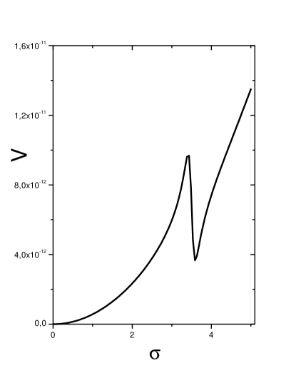
Figure 4: The effective potential for our second model. Note the similarity between this potential and that considered in Ref. re8 .

The Coleman-De Luccia instanton $\sigma(\tau)$ in this model is shown in Fig. 5. Our results are compared to that corresponding to the Einstein’s GR theory. Tunneling occurs from the initial point $\sigma_{i}\approx 3.54$, which almost coincides with the local minimum of V($\sigma$), to final point $\sigma_{f}\approx 3.31$. The evolution of the inflaton field during the tunneling process shown by Fig. 5 is quite similar to what happens in the previous case, but the values that the inflaton field gets immediately after the tunneling are different. The reason for this is due to the fact that we have consider $d\sigma/d\tau=0$, both at the beginning and at the end of the tunneling. Thus, at unlike of the first case, and in order to satisfy this condition in our second model, we were forced to consider different initial values of the inflaton field, when different values of the JBD parameter $\omega$ were taken.

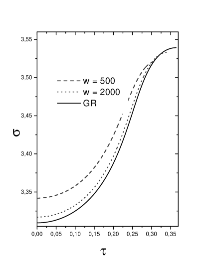
Figure 5: The instanton $\sigma(\tau)$ as a function of the Euclidean time $\tau$ for our second model in both Einstein’s GR and JBD theories (for $\omega=500$ and $\omega=2000$ in the latter case). Note the different values that occur for $\sigma$ at the beginning of inflation, i.e. at $\tau=0$. Again, as before, we have assumed $m=1$.

Figure 6 shows that almost everywhere along the evolution of the scalar inflaton field, $\sigma(\tau)$, it is found that $\mid\,V^{\prime\prime}\mid\,\gg\,H^{2}$. Unlike the previous case, the width of the peak increases when the $\omega$ parameter decreases.

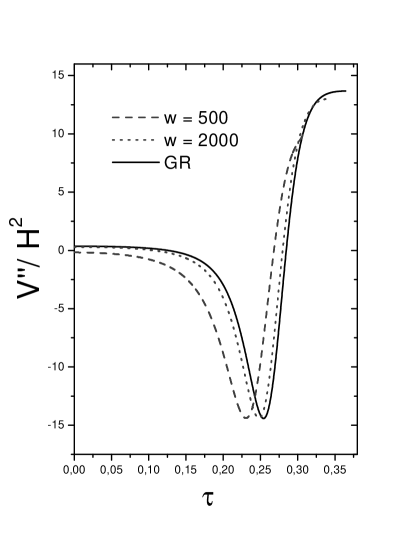
Figure 6: This graph shows how the inequality $\mid\,V^{\prime\prime}\,\mid\gg\,H^{2}$ is satisfied during the tunneling process. The continuous line represents what happen in Einstein’s GR theory. The other curves correspond to $\omega$=500 and $\omega$=2000 in JBD theory. We have assumed $m=1$.

In the following we are going to calculate the instanton action for the quantum tunneling between the false and the true vacuum in the JBD theory. By integrating by parts and using the Euclidean equations of motion, we find that the action may be written as

$$S\,=\,2\pi^{2}\,\int\,d\tau[a^{3}(\phi^{,\,2}+\sigma^{,\,2})-6\varepsilon\phi\,aa^{,}(a^{,}\phi+2a\phi^{,})].$$ (9)

Note that this action coincides with that corresponding to its analogous in the Einstein’s general relativity theory if we assume that $\epsilon\phi^{2}=Cte.=1/8\pi=1/\kappa^{2}$  Parker .

The $\sigma$ inflaton field is initially trapped in its false vacuum, whose value is $\sigma_{F}$, and where the JBD field has the value $\phi_{F}$. After tunneling to the true vacuum, the instanton and the JBD fields get the values $\sigma_{T}$ and $\phi_{T}$, respectively, and a single bubble is produced . Similar to the case of GR theory, the instanton (or bounce) action is given by $B=S-S_{F}$, i.e. the difference between the action associated with the bounce solution and the false vacuum. This action determines the probability of tunneling for the process. We have defined $V_{F}=V(\sigma_{F})$ and $V_{T}=V(\sigma_{T})$ as the false and true vacuum energies, respectively. Under the approximation that the bubble wall is infinitesimally thin, we obtain the reduced action for the thin-wall bubble:

$$S=2\pi^{2}S_{1}R^{3}-4\pi^{2}[(1-H_{F}^{2}R^{2})^{3/2}-1]\frac{\varepsilon\phi_{F}^{2}}{H_{F}^{2}}$$

$$\hskip 91.04872pt+\,4\pi^{2}[(1-H_{T}^{2}R^{2})^{3/2}-1]\frac{\varepsilon\phi_{T}^{2}}{H_{T}^{2}},$$ (10)

where we have taken into account the contributions from the wall (first term) and the interior of the bubble (the second and third terms). Here $R$ is the radius of the bubble, $H_{F}^{2}=V_{F}/3\varepsilon\phi_{F}^{2}$ and $H_{T}^{2}=V_{T}/3\varepsilon\phi_{T}^{2}$. The surface tension of the wall becomes defined by

$$S_{1}\,=\,\int\,d\tau\,[\,\phi_{wall}^{,\,2}\,+\,\sigma^{,\,2}\,],$$ (11)

or equivalently

$$S_{1}\,=\,\int\,d\tau\,\phi_{wall}^{,\,2}\,+\,\int_{\sigma_{T}}^{\sigma_{F}}d\sigma[2(V(\sigma)-V_{F})]^{1/2},$$

where $\phi_{wall}^{,}$ is the variation of scalar field $\phi$ across the bubble wall. To continue, we have taken the approach followed by the authors of Ref. Accetta , where they use the approximation $\phi_{wall}^{,}\approx 0$; in this way, we could drop the first term of Eq. (11). However, we should note that in our case we are concerned with the decay of a false vacuum with positive energy density to a true vacuum in which this energy is also positive, but smaller than the other one, i. e., the decay from $V(\sigma_{F})$ to $V(\sigma_{T})\neq 0$.

The curvature radius of the bubble wall is one for which the bounce action (10) is an extremum. Then, the wall radius is determined by setting $dS/dR$ = 0, which gives

$$\frac{S_{1}R}{2}=(1-H_{T}^{2}R^{2})^{1/2}\varepsilon\phi_{T}^{2}-(1-H_{F}^{2}R^{2})^{1/2}\varepsilon\phi_{F}^{2}.$$

This can be solved for the radius of the bubble, and it is found that

$$R=\left[\frac{S_{2}\pm(S_{2}^{2}-H_{2}[\,1-(\phi_{T}/\phi_{F})^{4}\,]\,)^{1/2}}{H_{2}}\right]^{1/2},$$ (12)

where $S_{2}$ is given by

$$S_{2}=\left(\frac{S_{1}}{2\varepsilon\phi_{F}^{2}}\right)^{2}\left[1+\left(\frac{\phi_{T}}{\phi_{F}}\right)^{4}\right]-\left[1-\left(\frac{\phi_{T}}{\phi_{F}}\right)^{4}\right][H_{T}^{2}-H_{F}^{2}],$$

and

$$H_{2}=\left[H_{F}^{2}-H_{T}^{2}\left(\frac{\phi_{T}}{\phi_{F}}\right)^{4}+\left(\frac{S_{1}}{2\varepsilon\phi_{F}^{2}}\right)^{2}\right]^{2}$$

$$\hskip 99.58464pt+\,H_{T}^{2}\,\left(\frac{\phi_{T}}{\phi_{F}}\right)^{4}\left(\frac{S_{1}}{\varepsilon\phi_{F}^{2}}\right)^{2}.$$

We choose the positive root in Eq. (12), since with this root we could get the appropriate Einstein’s General Relativity limit in which $\varepsilon\phi^{2}=\varepsilon\phi_{0}^{2}=Cte.\equiv 1/8\pi=1/\kappa^{2}$ with $\phi_{T}=\phi_{F}=\phi_{0}$. In this limit the curvature radius of the bubble wall becomes

$$R\longrightarrow\,R_{GR}=\frac{S_{1}\kappa^{2}}{([H_{F}^{2}-H_{T}^{2}+(S_{1}\kappa^{2}/2)^{2}]^{2}+H_{T}^{2}\kappa^{4}S_{1}^{2})^{1/2}}.$$

A dimensionless quantity $\Delta\,s$, which represents the strength of the wall tension in the thin-wall approximation, is given in the Einstein’s GR theory in ref. re8 , which in our case can be represented by

$$\Delta\,s=\,\frac{S_{1}\,R}{2\,\varepsilon\,\phi_{T}^{2}}\,<\,1.$$ (13)

By numerically solving the field equation associated with the JBD field $\phi$, Eq. (5), we obtain for $\omega=500$ the following values $\phi_{T}=7.645$ and $\phi_{F}=6.023$. With these values we find that $\Delta\,s=0,436$. Analogously, for $\omega=2000$, we obtain $\phi_{T}=17.247$ and $\phi_{F}=15.276$, and thus we get $\Delta\,s=0,429$. In the second model, it is found that, for $\omega=500$, $\phi_{T}=7.800$ and $\phi_{F}=5.220$, which gives $\Delta\,s=0,506$, and for $\omega=2000$, $\phi_{T}=17.310$ and $\phi_{F}=14.817$ we find $\Delta\,s=0,478$. We should note here that, as long as we decrease the value of the $\omega$ parameter the strength of the wall tension $\Delta\,s$ increases. We could see this from the fact that in the Einstein’s GR theory, $\triangle s$ becomes given by $\triangle s_{GR}=4\pi RS_{1}$ MSTTYY , which turns out to be smaller than the corresponding expression in the JBD theory, since the quantity $(\varepsilon\,\phi_{T}^{2}){-1}$ increases. In the first of the particular cases described above, we get that, when $\triangle s$ is compared with the corresponding value in the Einstein’s GR theory, we find that $\triangle s-\triangle s_{GR}\simeq$ 0.012, for $\omega=500$, and for $\omega$ = 2000 we get $\sim$ 0.005. In the second model this difference becomes of the order of $\sim 0.06$, for $\omega=500$ and $\sim 0.032$, for $\omega=2000$.

III Inflation after tunnelling

After the tunnel has occurred, we should both make an analytical continuation to the Lorentzian spacetime and see what is the time evolution of the scalar fields $\phi(t)$ and $\sigma(t)$, and of the scale factor $a(t)$. The field equations of motion for the fields $\sigma$, $\phi$ and $a$ are given by

$$\ddot{\sigma}\,=\,-3\,\frac{\dot{a}}{a}\,\dot{\sigma}\,-\,\frac{dV}{d\sigma}\,\,,$$ (14)

$$\ddot{\phi}=-3\frac{\dot{a}}{a}\dot{\phi}-\frac{\dot{\phi}^{2}}{\phi}-\frac{1}{1+6\varepsilon}\left[\frac{\dot{\sigma}^{2}}{\phi}-\frac{4}{\phi}V(\sigma)\right]\,\,,$$ (15)

and

$$\ddot{a}=2\frac{\dot{a}\dot{\phi}}{a\phi}-\frac{a}{3\varepsilon\phi^{2}}\left[\dot{\phi}^{2}+\frac{1+3\varepsilon}{1+6\varepsilon}\dot{\sigma}^{2}-\frac{1-6\varepsilon}{1+6\varepsilon}V(\sigma)\right],$$ (16)

where the dots now denote derivatives with respect to the cosmological time.

In order to numerically solve this set of Equations we use the following boundary conditions $\dot{\sigma}(0)=\dot{\phi}(0)=0$, $a(0)=0$ and $\dot{a}(0)=1$. In our first model the solutions $\sigma(t)$ are shown in Fig. 7 for some different values of the $\omega$ parameter. In the same situation, we have studied the evolution of the JBD field, $\phi$. We have found that this field monotonically increases to some constant value, which is closer to that determined by the actual value of the Planck mass, (recall that $\varepsilon\phi_{0}^{2}=1/8\pi$), just when the inflaton scalar field $\sigma$ begins to oscillate near the minimum of the effective potential, located at $\sigma\approx 0$. We have also found that for the range $50\leq\omega\leq 2000$, the universe could inflate more than the $60$ e-folding, which we find in Einstein’s theory of gravity. However, for a sufficiently small value of this parameter, say $\omega\approx 5$ or so, the e-folding obtained after tunneling has occurred, is not enough to solve the cosmological puzzles, such as flatness, horizon, etc. Therefore, we have found that our models are quite sensitive to the value we assign to the $\omega$ parameter.

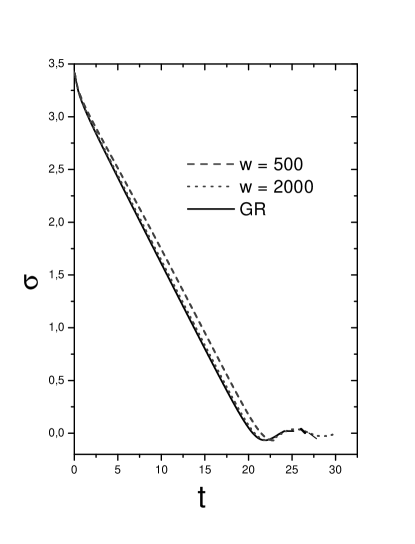
Figure 7: This plot shows the inflaton field $\sigma$ as a function of the cosmological time $t$ during the slow-rolls down open inflationary universe, either in the Einstein’s GR and JBD theories ($\omega$=500 and $\omega$=2000). In these graphs we have assumed the constant $m$ to be 1.

IV Scalar perturbation spectra

Even though the study of scalar density perturbations in open universes is quite complicated re8 , it is interesting to give an estimation of the standard quantum scalar field fluctuations inside the bubble for our scenarios. The corresponding density perturbation in the JBD theory becomes re1

$$\frac{\delta\,\rho}{\rho}\,\approx\,Cte\,H^{2}\left[\left(\varepsilon\phi^{2}8\pi\right)^{\frac{3}{2}}\,\frac{1}{|\dot{\sigma}|}\,+\frac{(1-\varepsilon\phi^{2}8\pi)}{2|\dot{\phi}|}\gamma\phi\right],$$ (17)

where $\displaystyle\gamma\,=\,\frac{1}{\sqrt{\omega+3/2}}$ and $Cte.\approx 3/5\pi$. The latter equation coincides with its analogous equation in Einstein’s theory, when the substitution $\varepsilon\phi^{2}=1/8\pi$ is made. The reason why this expression is approximated is because it is expected that other contributions to the exact expression exist re9 . However, as was observed by Linde re8 , we may use the above expression for $N>3$, as a correct result.

Figure 8 shows the magnitude of the scalar perturbations $\delta\rho/\rho$ for our first model as a function of the $N$ e-folds of inflation for two different values of the $\omega$ parameter, after the open universe was formed. Even though the shape of the graph is similar to the Einstein’s GR case, $\delta\rho/\rho$ has a maximum at small $N\sim O(12)$. Its maximum value, however, increases a little bit, when we decrease the $\omega$ parameter value. Similarly, the values of $N$ e-folds, where $\delta\rho/\rho$ vanishes, increase when $\omega$ decrease. We should mention that there is a relation between the value of the scalar perturbation and the $N$ e-folds of inflation. For $N\sim 10$, where $\delta\rho/\rho$ gets it maximum value, it is found that the scale where the scalar perturbation is measured corresponds to the $10^{24}cm$ scale. However, for $N\sim 15$ it decreases to $10^{22}cm$, and for $N\gg 50$ this practically comes to zero. We could show that something similar happens in the second model considered. There, the corresponding values of $N$ e-folds were smaller.

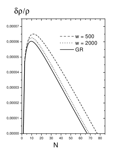
Figure 8: Scalar density perturbations for our first model produced inside the bubble N e-folds after the open universe creation. We have plotted $\delta\rho$/$\rho$ for $\omega=500$ and $\omega=2000$. These plots are compared with those obtained by using the Einstein’s GR theory, where $\delta\rho$/$\rho\approx\,CteH^{2}$/$|\dot{\sigma}|$

One interesting parameter to consider is the so-called spectral index $n$, which is related to the power spectrum of density perturbations $P^{1/2}_{\cal R}(k)$. For modes with wavelength much larger than the horizon ($k\ll aH$), the spectral index $n$ is an exact power law, expressed by $P^{1/2}_{\cal R}(k)\propto k^{n-1}$, where $k$ is the comoving wave number. In the slow roll limit, where $\ddot{\sigma}\simeq 0$ and the first two derivatives of the effective potential are small relative to its magnitude, i.e., $V^{\prime}$, $V^{\prime\prime}\ll V$, with $V^{\prime}=dV/d\sigma$, it is found that the spectral index $n$ is given by

$$n=1-4\epsilon+2\eta,$$

where the parameters $\epsilon$ and $\eta$, the so-called slow roll parameters are given by KoVa

$$\epsilon\simeq\frac{m_{Mp}^{2}}{16\pi}\left(\frac{V^{\prime}}{V}\right)^{2}\ll 1$$

and

$$\eta\simeq\frac{m_{Mp}^{2}}{8\pi}\left[\frac{V^{\prime\prime}}{V}-\frac{1}{2}\left(\frac{V^{\prime}}{V}\right)^{2}\right]\ll 1.$$

Figure 9 shows the spectral index parameter $n$ as a function of the e-folds parameter $N$ for two different values of the JBD parameter $\omega$. With the aim of comparing, we have also included here the spectral index in Einstein’s GR theory. Note that the parameter $n$ gets values which are, on average, smaller than that found in the Einstein theory.

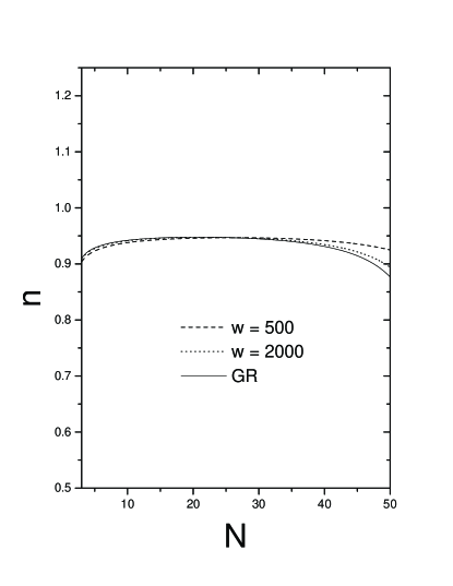
Figure 9: The spectral index $n$ as a function of the $N$ e-folds parameter for two different values of the JBD parameter $\omega$. The values that we have taken are $\omega=500$ and $\omega=2000$. These plots are compared with that obtained by using Einstein’s GR theory.

Certainly, apart from the scalar perturbations, tensor perturbation also exist. These perturbations are usually associated with perturbations of the bubble wall re6 . Specifically, in the Einstein’s GR theory it is known that the fluctuations of the bubble wall contribute to the low frequency spectrum of tensor perturbations, which can dominate over the scalar perturbations YaSaTa ; Ga ; Ga-Be . Here, we expect something similar to occur in our models, except at low enough JBD parameter, where the Einstein’s GR and the JBD theories can be distinguished one from the other. However, due to present bound of the observational limits from the solar system measurements for the $\omega$ parameter Wi , we expect these contributions to become tiny corrections of that obtained in the Einstein’s GR theory. Certainly, this latter point deserves further investigation that we hope to carry out in a near future.

V conclusion

Since we still we do not know the exact value of the $\Omega$ parameter, it is convenient to count on an inflationary universe model in which $\Omega<1$. In this sense, we could have single-bubble open inflationary universe models, which may be consistent with a natural scenario for understanding the large scale homogeneity and isotropy structure. However, open inflationary models have a more complicated primordial spectrum than that obtained in flat universes, where extra discrete modes and possibly large tensor anisotropies spectrum could be found, especially those related to supercurvature modes, which are particular to open inflationary universes. Forthcoming astronomical measurements will determine if this extra terms are present in the scalar spectrum.

In this paper we have studied one-field open universe models in which the gravitational effects are described by a JBD theory. In this theory the fundamental quantity is the JBD field $\phi$, from which, after that universe enters the Lorentzian era, it can numerically be shown that it monotonically increases from an initial value to the present value of the Planck mass obtained at the end of inflation. We have studied solutions to two effective potentials in which the CDL instantons exist. The existence of these instantons is shown because the inequality $|V^{{}^{\prime\prime}}|>H^{2}$ is satisfied, and thus, slow-roll inflationary universes are realized for different values of the JBD $\omega$ parameter.

For the two models considered, $V^{{}^{\prime\prime}}$ remains greater than $H^{2}$ during the first e-folds of inflation. In the thin-wall limit we have also found an increase in the strength of the wall tension, $\triangle s$, when compared with their analogous results obtained in the Einstein’s GR theory.

Since in $\delta\rho/\rho$ graphs the maximum present a small displacement in the JBD theory, when compared with that obtained in the Einstein’s GR theory, this would change the constraint on the value of the parameter $m$ that appears in the scalar potentials. In this way, we have shown that one-field open inflationary universe models can be realized in the JBD theory.

- (1) A. Guth, Phys. Rev. D 23, 347 (1981).
- (2) A. Albrecht and P. Stainhardt, Phys. Rev. Lett. 48, 1220 (1982).
- (3) A. Linde, Phys. Lett. B 108, 389 (1982).
- (4) M Sasaki, T. Tanaka, K. Yamamoto and J. Yokoyama, Phys. Lett. 317B, 510 (1993).
- (5) M. Bucher et al, Phys. Rev. D 52, 3314 (1995); M. Bucher and N. Turok, Phys. Rev. D 52, 5538 (1995).
- (6) A. Linde, Phys. Lett. B, 351, 99 (1995); A. Linde and A. Mezhlumian, Phys. Rev. D 52, 6789 (1995).
- (7) A. Linde, Phys. Rev. D 59 , 023503 (1998).
- (8) J.R. Gott, Nature 295, 304 (1982).
- (9) J.R. Gott and T.S. Statler, Phys. Lett. 136B, 157 (1984).
- (10) U. Moschella and R. Schaeffer, Phys. Rev. D 57, 2147 (1998).
- (11) M. Bouchmadi and P. F. González-Días, Phys. Rev. D 65, 063510 (2002).
- (12) K. Enquist,H. Kurki-Suonio and J. Väliviita, Phys. Rev. D 65, 043002 (2002).
- (13) S. Coleman and F. De Luccia, Phys. Rev. D 21 , 3305 (1980).
- (14) A. Linde, M. Sasaki and T. Tanaka, Phys. Rev. D 59, 123522 (1999).
- (15) B. Ratra and P.J.E. Peebles, Astrophys. J. 432, L5 (1994); Phys. Rev. D 52, 1837 (1995).
- (16) T. Chiba and M. Yamaguchi, Phys. Rev. D 61, 027304 (2000).
- (17) P. Jordan, Z. Phys.157, 112 (1959); C. Brans and R. Dicke, Phys. Rev. 124, 925 (1961).
- (18) S. Parker, Phys. Lett. 121B, 313 (1983).
- (19) F. Accetta and P. Romanelli, Phys. Rev. D 41, 3024 (1990).
- (20) M. Sasaki, T. Tanaka and Y. Yakushige, Phys. Rev. D 56, 616 (1997).
- (21) A. Starobinsky and J. Yokoyama, gr-qc/9502002.
- (22) E. W. Kolb and S. L. Vadas, Phys. Rev D 50, 2479, (1994); For a review, see J. E. Lidsey, A. R. liddle, E. W. Kolb, E. J. Copeland, T. Barbiero and M. Abney, Rev. Mod. Phys. 69, 373 (1997); D. H. Lyth and A. Riotto, Phys. Rep. 314, 1, (1999).
- (23) K. Yamamoto, M. Sasaki and T. Tanaka, Phys. Rev. D 54, 5031 (1996).
- (24) J. Garriga, Phys. Rev. D 54, 4764 (1996).
- (25) J. Garcia-Bellido, Phys Rev. D 56,3225 (1997).
- (26) C. M. Will, Living Rev. Rel. 4, 4 (2001).