A new recipe for causal completions

Abstract:

We discuss the asymptotic structure of spacetimes, presenting a new construction of ideal points at infinity and introducing useful topologies on the completed space. Our construction is based on structures introduced by Geroch, Kronheimer, and Penrose and has much in common with the modifications introduced by Budic and Sachs as well as those introduced by Szabados. However, these earlier constructions defined ideal points as equivalence classes of certain past and future sets, effectively defining the completed space as a quotient. Our approach is fundamentally different as it identifies ideal points directly as appropriate pairs consisting of a (perhaps empty) future set and a (perhaps empty) past set. These future and past sets are just the future and past of the ideal point within the original spacetime. This provides our construction with useful causal properties and leads to more satisfactory results in a number of examples. We are also able to endow the completion with a topology. In fact, we introduce two topologies, which illustrate different features of the causal approach. In both topologies, the completion is the original spacetime together with endpoints for all timelike curves. We explore this procedure in several examples, and in particular for plane wave solutions, with satisfactory results.

1 Introduction

In many situations, important physical questions about spacetimes are concerned with what happens ‘at the boundary.’ For example, in cosmology the classical spacetime modeling our universe has an initial singularity, and it is important to understand how a more complete theory assigns initial conditions in the region where curvatures become large. In scattering experiments, the experimentalist specifies a collection of ingoing particles at large distances and early times, and measures a collection of outgoing particles at late times. More generally, to study non-compact spacetimes in quantum theories of gravity, we must impose some restrictions on the asymptotic behaviour of the metric and other fields. In all these cases, the spacetime is a manifold, and so does not have a real boundary. A technique which allowed us to equip a spacetime $M$ with a boundary in some abstract sense, defining some suitable completion $\bar{M}$, would provide a useful tool in addressing such problems.

This is a long-studied issue; Penrose provided the first successful construction of such a boundary in his characterisation of asymptotically simple spacetimes [1] almost 40 years ago. Asymptotically simple spacetimes model the behaviour of isolated weakly-gravitating sources. A manifold $M$ with metric $g$ is said to be asymptotically simple if there exists a strongly causal space $(\tilde{M},\tilde{g})$ and an imbedding $\theta:M\to\tilde{M}$ which imbeds $M$ as a manifold with smooth boundary $\partial M$ in $\tilde{M}$, such that:

1. There is a smooth function $\Omega$ on $\tilde{M}$ such that $\Omega>0$ and $\Omega^{2}g=\theta_{*}(\tilde{g})$ on $\theta(M)$,

2. $\Omega=0$ and $d\Omega\neq 0$ on $\partial M$,

3. every null geodesic in $M$ has two endpoints on $\partial M$.

This definition associates a boundary with $M$ in a well-defined mathematical sense. Furthermore, it extends the conformal structure on $M$ (the metric up to conformal transformations) to a conformal structure on $\bar{M}=M+\partial M$. Thus, we can say quite a bit about how a particular point on $\partial M$ is related to points of $M$; it is these relations which are important for studying physical questions.

In [2], Geroch, Kronheimer and Penrose (GKP) proposed a different approach to adding a boundary to spacetime. This approach, which will be reviewed in more detail in section 2.1, is based on the causal structure of spacetime. Basically, one characterises points of the spacetime in terms of the timelike curves which end on them. One can then extend the spacetime by adding endpoints to timelike curves for which they do not already exist. In particular, two curves $\gamma_{1}$, $\gamma_{2}$ are given the same future endpoint if $I^{-}[\gamma_{1}]=I^{-}[\gamma_{2}]$ (and similarly with past and future interchanged). This approach is based on the causal structure of spacetime, so we only get causal (and not conformal) relations between the new boundary points, dubbed ‘ideal points’, and the original spacetime. This relaxing of the structure gets us several advantages over asymptotic simplicity in exchange. The causal approach yields a procedure for constructing the boundary, whereas the conformal approach provides no algorithm for constructing an appropriate $(\tilde{M},\tilde{g})$ satisfying properties 1-3 above. In addition, the causal approach may be applied to arbitrary strongly causal spacetimes, whereas the conformal approach requires conformal flatness at large distances – a condition which covers many spacetimes of physical interest but remains a severe restriction on the space of all metrics.

However, there is an important technical difficulty with the causal approach. In [2], it was pointed out that we cannot regard all the future endpoints we add to curves as distinct from all the past endpoints; some ideal points can act as both the future and past endpoints of timelike curves. Thus, GKP [2] and succeeding authors suggested that identifications be made between the future and past endpoints, and that the ideal points should be equivalence classes generated by some relation.

GKP [2] proposed that these identifications should be obtained by first introducing a topology and then imposing the minimum set of identifications necessary to obtain a Hausdorff space. However, this construction fails to produce the ‘obvious’ completion in some examples [3, 4]. Attempts have been made in the past to modify the topology to produce more satisfactory results [5], but these modifications also fail in some examples [6]. In part, this is because the introduction of an appropriate topology is itself problematic in the causal approach. An approach to the identifications based more directly on the causal structure was introduced by Budic and Sachs [7] and further refined by Szabados [8, 9]. We review Szabados’ rule for performing identifications in section 2.2, using a slightly different language and notation. These causal approaches produce more ‘natural’ identifications, reproducing the intuitive point-set structure for $\bar{M}$ in various examples.

However, the construction of $\bar{M}$ from equivalence classes suffers from a fundamental difficulty: it has not been possible to give a general definition of the timelike pasts and futures of points in $\bar{M}$ which will always agree with that on $M$. The identifications can introduce causal relations between points of $M$ not present in the original spacetime, thus altering the structure on which the causal approach is itself based. The problem arises when one attempts to turn a natural relation $R_{pf}$ between past and future endpoints of curves into an equivalence relation by enforcing transitivity by hand.

These approaches thus fail in an essential way. If we compare the logic of the causal approach to that of the conformal approach, requiring that the notions of $I^{\pm}(p)$ extend from $M$ to $\bar{M}$ is analogous to the requirement that $\tilde{M}$ have a metric conformal to the metric on $M$. Thus, we feel that any construction which fails to satisfy this property should not properly be described as a causal completion. This suggests that radical revision of the construction of $\bar{M}$ may be necessary.

In section 2.3, we will propose a new approach to the construction of $\bar{M}$, which is not based on a quotient. In our approach, points of $\bar{M}$ are constructed from naturally related IP-IF pairs. The idea is that every point of $M$ has both a past and a future, and while considering just one or the other uniquely specifies the point, it does not fully exploit the information in the causal structure. Thus, we adopt an approach where points of $\bar{M}$ are specified by giving both their past and future (for ideal points, one or the other may be empty). We construct pairs from IPs and IFs that are related through the same relation $R_{pf}$ used in [8]. Thus, the key difference between our approach and previous approaches is that we avoid completing this to an equivalence relation—a step that has nothing to do with the causal structure.

The IP-IF pair directly determines the past and future of the associated point of $\bar{M}$. This tighter connection between the ideal points and the primitive structures allows us to prove that the completion $\bar{M}$ will always have a chronology relation (i.e., a notion of timelike past and futures) which is compatible with that on $M$. Thus, this definition of $\bar{M}$ satisfies what we regard as the key criterion for a causal completion. The necessary chronology relation is discussed in section 3.1. We also discuss the construction of a causality on $\bar{M}$ in section 3.2. Here the situation is somewhat less satisfactory, as different apparently reasonable notions of causality present themselves. However, as the construction is based on timelike, and not causal, pasts and futures, we view the causality as less important than the chronology.

Another important issue is the construction of a suitable topology on $\bar{M}$. Since we want to use the ideal points to represent asymptotic, or limiting, behaviour at large distances in spacetime, we need a suitable topology to tell us what limits in the bulk spacetime $M$ approach which ideal points in $\bar{M}$. Of course, we want these limits to be compatible with our causal structure. We therefore want to introduce a topology on $\bar{M}$ such that $\bar{M}$ corresponds to $M$ equipped with a suitable boundary in the topological sense, and such that the TIP $I^{-}[\gamma]$ and TIF $I^{+}[\gamma]$ are limit points of the curve $\gamma$. While the original approach of Geroch, Kronheimer and Penrose [2] was based on the further assumption that the topology was Hausdorff, this strong assumption is sacrificed in the approaches based more directly on causality [7, 8, 9].

In the quotient constructions, the topology adopted was essentially that introduced by Geroch, Kronheimer and Penrose [2], perhaps with small refinements. This topology is basically constructed by introducing a suitable ‘generalised Alexandrov’ topology on the space of all IPs and IFs, and adopting the quotient topology on the space $\bar{M}$ obtained after identifying the members of an equivalence class. This construction allows one to define a topology satisfying the basic requirements above, but it does not always give the expected relations between limits and ideal points in simple examples. Some examples of these difficulties were discussed in [3, 4, 6], and similar issues arise even in de Sitter space and anti-de Sitter space.

Our change from identifications to pairs requires a new definition of the topology. The construction of a topology remains a difficult and subtle issue. Given our focus on chronology, one might think the most natural thing to do is to adopt an Alexandrov topology, based on the timelike pasts and futures defined in $\bar{M}$. However, this does not define a strong enough topology to give suitable open neighbourhoods of all ideal points. We will therefore work with topologies which are based more indirectly on the causal structure. We face some of the same difficulties as earlier authors, and we do not find a unique topology which yields intuitively appealing results in all examples. Instead, we will explore two different definitions of the topology, representing different implementations of the same basic idea.

We introduce a topology $\bar{\cal T}$ in section 4. We introduce a new structure on which to base the topology, using the causal structure to define sets $L^{\pm}(\bar{S})$ which it is appropriate to regard as the closure in $\bar{M}$ of $I^{\pm}_{C}(\bar{S})$ for arbitrary $\bar{S}\subset\bar{M}$. We then define a topology on $\bar{M}$ by requiring that the sets $\bar{M}\setminus L^{\pm}(\bar{S})$ are open. We show that in this topology, $\bar{M}$ does correspond to $M$ equipped with a boundary in the topological sense, and that ideal point pairs containing $I^{\pm}[\gamma]$ are limit points of the timelike curve $\gamma$. We show that this topology has fairly good separation properties; failure of the expected separation of ideal points occurs only in well-controlled examples. On the other hand, some sequences of points in $M$ will fail to have the intuitively expected limit points in $\bar{M}$. This motivates us to consider a modified topology $\bar{\cal T}_{alt}$ in appendix B, in which we use a different definition of the sets $L^{\pm}(\bar{S})$. This modified topology leads to more limit points in interesting examples, but it goes a bit too far and has weaker separation properties. These two topologies share some desirable features: both satisfy the minimal requirements enunciated above, and they yield the standard topology on the completion for both de Sitter and anti-de Sitter space.

As was remarked in [2], one does not have any sense in the abstract of what is the correct completion of a spacetime $M$. In judging a proposed completion, applying our intuition to simple examples is an important source of guidance. Such examples have played an important part in the previous literature on this subject [3, 4, 6]. We will use several simple toy examples to illustrate the different aspects of the construction as we go along. Once we have developed the techniques, we will apply them to the construction of the causal boundary for plane waves. Plane waves provide an important ‘real-world’ example where the full power of the causal approach is needed to obtain an asymptotic boundary. In section 5 we find that, using these purely causal methods, one may recover the result (previously announced in [11]) that the causal boundary of a homogeneous plane wave is a null line segment. A careful application of the original definition of [2] gives a different answer, illustrating the importance of these subtleties.

Due to the length of time which has passed since the works [2, 7, 8] on which we build, we have tried to make this paper reasonably self-contained. Although we have assumed familiarity with the basic ideas of causality commonly used in general relativity, it is hoped that the interested reader having no previous familiarity with the specifics of causal completions will be able to understand our discussion without reference to the previous literature. We have not reviewed all the previously proposed constructions in detail, but we have tried to state the differences in their actions on the examples in a way that does not assume a knowledge of these details.

2 Construction of a causal completion $\bar{M}$

Following previous works, we first assume that the spacetime is strongly causal; this seems to be the weakest assumption allowing us to construct a causal completion $\bar{M}$ in general. A strongly causal spacetime is a spacetime in which, for every $x\in M$, there is a neighborhood $U\ni x$ which no non-spacelike curve enters more than once. Strong causality implies that the spacetime is past- and future-distinguishing i.e., $I^{-}(p)=I^{-}(q)$ iff $p=q$, and $I^{+}(p)=I^{+}(q)$ iff $p=q$, for any points $p,q\in M$. This means that we can associate any point $p$ in $M$ with its chronological past and future $I^{\pm}(p)$ in a one-to-one way.

2.1 IPs and IFs

The set $I^{-}(p)$ is an example of a past-set: a set which is the past of some set. In fact, $I^{-}(p)$ is an indecomposable past-set, or IP. This means it cannot be expressed as the union of two proper subsets which are themselves past-sets. If we think of the spacetime in terms of its causal structure, these indecomposable past-sets can be thought of as the elementary objects from which the causal structure is built.

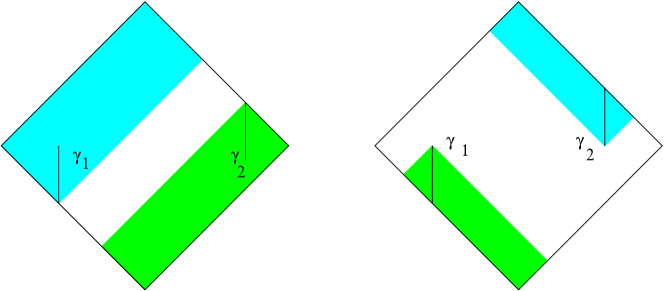
Figure 1: On the left, a conformal diagram of 1+1 Minkowski space showing the TIF $I^{+}[\gamma_{1}]$ and TIP $I^{-}[\gamma_{2}]$. On the right, the PIP $I^{-}[\gamma_{1}]$ and PIP $I^{-}[\gamma_{2}]$ are shown.

So every point $p\in M$ determines an IP $I^{-}(p)$. However, the converse is not true: there are IPs which are not of the form $I^{-}(p)$ for some $p\in M$. But Geroch, Kronheimer and Penrose showed [2] that every IP is of the form $I^{-}[\gamma]$ for some timelike curve $\gamma$ in $M$, and that all such $I^{-}[\gamma]$ are IPs. Thus, the set of IPs is the set of chronological pasts $I^{-}[\gamma]$ for all timelike curves $\gamma$ in $M$. If the curve $\gamma$ has a future endpoint $p$, $I^{-}[\gamma]=I^{-}(p)$, the IP is termed a proper IP, or PIP. If $\gamma$ is future-endless, the IP $I^{-}[\gamma]$ is a terminal IP, or TIP. We call the set of IPs $\hat{M}$. Elements of this set are denoted by undecorated capital letters, $P\in\hat{M}$.

One can similarly define future-sets, indecomposable future-sets (IFs), PIFs and TIFs. The set of IFs is called $\check{M}$. Elements of this set will be written with stars, $P^{*}\in\check{M}$.

The idea is to construct the ideal points from the TIPs and TIFs; that is, we construct the additional points in terms of the spacetime regions they can physically influence or be influenced by. Put another way, we will add endpoints to endless timelike curves, in such a way that two curves go to the same future (past) point if they have the same past (future). Thus, we think of $\hat{M}$ as a partial completion of $M$, which adjoins as ideal points the ‘future endpoints’ of all future-endless timelike curves $\gamma$. If the spacetime $M$ is geodesically incomplete, the ideal points associated with incomplete geodesics will represent singularities, so the ideal points can represent both singularities and points at infinity.

Although this procedure does not give us as much structure as the method of conformal rescaling, the fact that it is constructive is a considerable advantage. Since we construct $\hat{M}$ directly from $M$, this method is universally applicable. In contrast, conformal compactification makes the assumption that a suitable conformally-related manifold $\tilde{M}$ exists. This assumption can fail, and even if such an $\tilde{M}$ exists, we have no general algorithm for obtaining it. Finally, although uniqueness of the conformal approach in the asymptotically simple context was shown in [1], it need not be unique more generally. But in the causal approach the construction of $\hat{M}$ is a straightforward exercise in studying the causal structure, and the only assumption is strong causality. This method also allows us to study singular points on the same footing as points at infinity, which is not possible in the conformal compactification.

2.2 Quotient constructions

Clearly what we have constructed so far are only partial completions; we should wish to adjoin both the past and future ideal points, that is, both the TIPs and TIFs, in constructing our completion $\bar{M}$. Since there is a natural mapping $M\to\{\hat{M},\check{M}\}$, conveniently referred to as $I^{\mp}$, which sends $p\to\{I^{-}(p),I^{+}(p)\}$, one might try to construct a completion which adjoins all TIPs and TIFs by considering the set

$$M^{\sharp}=(\hat{M}\cup\check{M})/R,$$ (1)

where $R$ identifies every PIP $I^{-}(p)$ with the corresponding PIF $I^{+}(p)$. Elements of $M^{\sharp}$ will be written as $P^{\sharp}$. However, this will overcount the ideal points; in some cases, there will be timelike curves in $M$ which approach a given ideal point from both the past and the future (this happens, for example, for the conformal boundary of anti-de Sitter space, or on the vertical segment of the triangle $R_{1}$ in the example of figure 2). In an approach based on identifications, some TIPs and TIFs must also be identified.

In [2], additional identifications between TIPs and TIFs were obtained by introducing a topology on the $M^{\sharp}$ defined above and making further identifications as required to obtain a Hausdorff space. Apart from practical problems with the specific implementation in [2] which have been extensively discussed in the literature [3, 4, 5, 8, 6], this topological approach has two conceptual defects: it makes the connection between the identifications and the causal structure rather indirect, and it introduces an additional assumption, that the correct completion will be Hausdorff in this topology. Although this might at first seem an entirely reasonable assumption, there is no natural reason to impose any such a priori restriction on the completion for arbitrarily complicated $M$. In fact, an example (see figure 5) was introduced in [2] for which $\bar{M}$ cannot simultaneously be Hausdorff, have the intuitively expected limiting ideal points for sequences in $M$, and have a chronology compatible with that of $M$.

As a result, Budic and Sachs [7] proposed to construct the identifications between TIPs and TIFs in a different way. They modified the quotient construction (1) by finding an appropriate identification $R$ which can act on any IPs and IFs, and whose action on PIPs and PIFs is equivalent to that used in (1). One wishes to identify IPs and IFs if they are the past and future of ‘the same point’. Thus, one regards the identification used in (1) as a two-step process, first introducing a notion of the ‘future’ of a PIP $P=I^{-}(p)$ as the set $f(P)=I^{+}(p)$, and similarly defining the ‘past’ of a PIF $P^{*}=I^{+}(p)$ as the set $p(P^{*})=I^{-}(p)$, and then identifying an IP $P$ with an IF $Q^{*}$ if $f(P)$ is appropriately related to $Q^{*}$ and $p(Q^{*})$ is appropriately related to $P$.

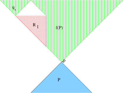
Figure 2: An example which illustrates important subtleties in dealing with the causal completion. The spacetime is constructed by excising the closed triangular region $R_{1}$ from two-dimensional flat space. If we consider a point $p$ on the diagonal null line, the PIP $P=I^{-}(p)$ provides an example where $f(P)$ is not an IF. Also, the points $p$ and $q$ are causally related in $\bar{M}$, but not in $M$.

Given a past-set $P$, a natural notion of the associated future-set is the ‘common future’, that is, the set of points to the future of all points $p\in P$. More formally, define $f(P)$ for any IP $P$ by

Definition 1

The common future $f(P)$ for any IP $P$ is

$$f(P)=\cup_{x}I^{+}(x):x\in M,P\subset I^{-}(x).$$ (2)

That is, $f(P)$ is the union of the futures of all points $x\in M$ such that $x$ is to the future of all points in $P$. This can be rewritten in several equivalent ways:

$$f(P) = I^{+}[\{x\in M:P\subset I^{-}(x)\}]$$ (3)

$$= I^{+}[\cap I^{+}(p):p\in P]$$ (4)

$$= Int[\cap I^{+}(p):p\in P],$$ (5)

where $Int$ denotes the topological interior of a set in $M$. The set $f(P)$ so defined is by definition a future-set; however, it is not necessarily an indecomposable future-set (see figure 2 for a counterexample). The common past $p(P^{*})$ of the future set $P^{*}$ is defined similarly.

In [7], the spacetime $M$ was restricted to be causally continuous, which means that $I^{\pm}(p)$ will vary continuously (as a point-set in $M$) whenever $p$ does. This restriction was meant to eliminate all the examples where $f(P)$ is not an IF (in fact, it does not quite do so; see [12] for a counterexample), and [7] then basically defined $R$ to identify $P$ with $Q^{*}$ iff $f(P)=Q^{*}$ and $P=p(Q^{*})$.

This approach was extended by Szabados [8], who introduced a more subtle identification which successfully addresses examples such as figure 2. We present his idea in two stages. First consider the following relation

Definition 2

Let $R_{pf}\subset\hat{M}\times\check{M}$ be the set of pairs of the form $(P,Q^{*})$ for which $Q^{*}$ is a maximal subset of $f(P)$ and $P$ is a maximal subset of $p(Q^{*})$; i.e., satisfying

$$Q^{*}\subset f(P);\quad\nexists R^{*}\in\check{M}:R^{*}\neq Q^{*},Q^{*}\subset R^{*}\subset f(P).$$ (6)

and

$$P\subset p(Q^{*});\quad\nexists R\in\hat{M}:R\neq P,P\subset R\subset p(Q^{*}).$$ (7)

Now consider $\bar{R}_{pf}$, the smallest equivalence relation on $\hat{M}\cup\check{M}$ which identifies every IP $P$ and IF $Q^{*}$ for which $(P,Q^{*})\in R_{pf}$. Szabados’ idea [8] is then equivalent to the following identification:

Definition 3

Given $M$, the causal completion $\bar{M}_{id}$ is

$$\bar{M}_{id}=(\hat{M}\cup\check{M})/\bar{R}_{pf}.$$ (8)

Note that if $f(P)$ is an IF, the above condition reduces to $f(P)=Q^{*}$, in which case they are the same as those of [7]. The subscript $id$ refers to the construction through the identifications imposed on points in $\hat{M}\cup\check{M}$. An important theorem proven in [8] (his Proposition 5.1) is

Theorem 1

For each point $q\in M$, the identification $\bar{R}_{pf}$ used in the preceding definition identifies $I^{+}(q)$with $I^{-}(q)$ but with no other IPs or IFs.

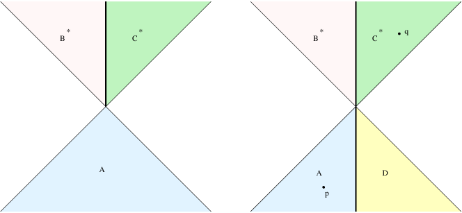
Figure 3: An example (left) where more than one TIF is identified with a TIP. We excise the line $x=0$, $t\geq 0$ from two-dimensional flat space. The TIP $A$ and TIFs $B^{*}$, $C^{*}$ all correspond to the same ideal point. A trouble-free but suggestive example in which we consider the IPs and IFs in the interior of an excised line segment appears on the right.

Thus, the identification $\bar{R}_{pf}$ will reproduce precisely the identification $R$ used to construct $M^{\sharp}$ in (1), together with some additional identifications that involve only TIPs and TIFs. This property is a good start. Note, however, that while each PIP is identified with exactly one PIF and vice-versa, the same need not apply to TIPs and TIFs; the left spacetime in figure 3 illustrates an example where more than one TIF is identified with a TIP. This property turns out to be quite dangerous. It implies that the future of an ideal point in this approach is not always an IF; as illustrated by the 2+1 dimensional example in appendix A, the addition of ideal points can introduce new causal relations between elements of $M$.

While the 2+1 dimensional example in appendix A is not overly complicated, we know of no useful 1+1 analogue. Thus it cannot be summarized by a simple picture and its description is somewhat involved. However, the basic flavor can be obtained by consulting figure 3. In the example on the left, the pairs $(A,B^{*}),(A,C^{*})\in R_{pf}$ force the identification of $B^{*}$ and $C^{*}$, though these two future sets have little in common. In contrast the example on the right has only $(A,B^{*}),(D,C^{*})\in R_{pf}$, and $B^{*}$ is not identified with $C^{*}$. Note, however, that if for some reason $B^{*}$ and $C^{*}$ were identified then a causal link would be introduced between $p$ and $q$ even though $q\notin I^{+}(p)$; the new ideal point would naturally be thought of as lying chronologically between $p$ and $q$ and forming a new causal link. The 2+1 dimensional example in appendix A achieves essentially this result through the use of a fifth region $E$. In sufficiently complicated examples the introduction of such new causal links can create closed timelike curves in the completed manifold. We find this property unsatisfactory, as it destroys the very structure on which the causal completion was built.

2.3 Ideal points as IP-IF pairs

Our main purpose in this paper is to introduce a new approach to the construction of the causal completion $\bar{M}$ from the primitive data about the causal structure of the spacetime encoded in $\hat{M}$ and $\check{M}$. The basic idea is that we want to get back to thinking of the TIPs and TIFs as the pasts and futures of ideal points. That is, we want to define elements of $\bar{M}$ in such a way that the past (in $M$) of any element of $\bar{M}$ is either some element of $\hat{M}$, or is empty. As we have seen above, this will not be true in an approach based on equivalence classes when one considers a reasonably general class of spacetimes including, e.g., the left example in figure 3.

As a result, we advocate a different construction. We will define an element $\bar{P}$ of $\bar{M}$ in terms of an IP $P$ and an IF $P^{*}$. Later, we will interpret $P$ and $P^{*}$ as the intersection with $M$ of the past and future of $\bar{P}$. We adopt the same relation $R_{pf}$ defined in definition 2 to relate pasts and futures, but use $R_{pf}$ directly instead of completing it to an equivalence relation $\bar{R}_{pf}$:

Definition 4

Given $M$, the causal completion $\bar{M}$ consists of all those pairs $(P,P^{*})$ such that

1. $(P,P^{*})\in R_{pf}\subset\hat{M}\times\check{M}$, or

2. $P=\emptyset$ and $P^{*}$ does not appear in any pair in $R_{pf}$, or

3. $P^{*}=\emptyset$ and $P$ does not appear in any pair in $R_{pf}$.

Note that every IP $P$ or IF $P^{*}$ appears in at least one pair; they may appear in more than one such pair, though those that appear in pairs of the form $(P,\emptyset)$ or $(\emptyset,P^{*})$ appear in only one pair.

Elements of $\bar{M}$ will be written as $\bar{P}=(P,P^{*})$. In discussing some element $\bar{P}$, we will write $P,P^{*}$ to mean the elements of the pair. Note that theorem 1 guarantees that, for $p\in M$, the sets $I^{\pm}(p)$ each appear in exactly one pair in $\bar{M}$, and that they appear together. Thus there is a natural injective map $\Phi:M\to\bar{M}$, $\Phi(p)=(I^{-}(p),I^{+}(p))$.

In the example on the left of figure 3, instead of having a single ideal point whose past is $A$ and whose future is $B^{*}\cup C^{*}$, we will have two ideal points $(A,B^{*})$ and $(A,C^{*})$. We feel that this is a more natural result from the point of view of the causal structure; there is nothing about the causal structure that requires these two points be identified—there is no relation between $B^{*}$ and $C^{*}$—and it is useful to record the information about the separate relations between $A$ and $B^{*}$ and $A$ and $C^{*}$ in the causal completion. If one feels that consideration of the causal structure alone produces a rather ‘big’ completion, the resulting $\bar{M}$ can always be used as a starting-point for further identifications, should they seem desirable for some other reason.

3 Causal structure on $\bar{M}$

Since the causal structure is of primary importance, one would like to see to what extent the causal structure on $M$ extends to $\bar{M}$. A general axiomatic definition of a causal space was given in [13]:

Definition 5

A set $M$ together with three relations $\prec$, $\ll$ and $\to$ is called a causal space if the relations satisfy the following conditions:

1. $x\prec x$,

2. $x\prec y$ and $y\prec z$ implies $x\prec z$,

3. $x\prec y$ and $y\prec x$ implies $x=y$,

4. Not $x\ll x$,

5. $x\prec y$ and $y\ll z$ implies $x\ll z$,

6. $x\ll y$ and $y\prec z$ implies $x\ll z$,

7. $x\to y$ iff $x\prec y$ and not $x\ll y$.

The relations are collectively called the causal relations; $\prec$ is called the causality, $\ll$ is called the chronology, and $\to$ is called the horismos. If we have two relations satisfying the relevant conditions, we can use them to define the third; for example, we can regard the last condition as defining the horismos.

Before discussing the causal structure for $\bar{M}$, let us review some results of [2], where it was shown that we can make the set $\hat{M}$ a causal space by introducing a causality and chronology specified by

$$P\prec_{IP}Q\quad\mbox{iff }P\subset Q,$$ (9)

$$P\ll_{IP}Q\quad\mbox{iff }P\subset I^{-}(q)\mbox{ for some }q\in Q.$$ (10)

They showed that when $P$ and $Q$ are PIPs, these relations include the relations between $p$ and $q$ as points of $M$. That is, $p\prec q$ implies $I^{-}(p)\prec_{IP}I^{-}(q)$, and $p\ll q$ implies $I^{-}(p)\ll_{IP}I^{-}(q)$. One says that the map $I^{-}$ preserves the chronology and the causality. However, $p$ and $q$ in figure 2 show that the inverse statements do not hold. There, $p\prec_{IP}q$ since $I^{-}(p)\subset I^{-}(q)$, but we do not have $p\prec q$. In addition, $p\ll_{IP}q$ but we do not have $p\ll q$. Thus, this causality and chronology can involve additional relations even between PIPs. This suggests that it is necessary to consider both pasts and futures to construct a good chronology.

We can similarly define causality and chronology on $\check{M}$, using $Q\prec_{IF}P$ if $P\subset Q$, $Q\ll_{IF}P$ if $P\subset I^{+}(q)$ for some $q\in Q$.

3.1 Chronology on $\bar{M}$

Let us now proceed to consider $\bar{M}$. There is a natural chronology on $\bar{M}$:

Theorem 2

The relation $\ll_{C}$ on $\bar{M}$ defined by

$$\bar{P}\ll_{C}\bar{Q}\quad\mbox{iff }P^{*}\cap Q\neq\emptyset.$$ (11)

is a chronology on $\bar{M}$.

Proof: To show transitivity, suppose $\bar{P}\ll_{C}\bar{Q}$ and $\bar{Q}\ll_{C}\bar{R}$. Since $\bar{P}\ll_{C}\bar{Q}$, there is an $s\in P^{*}\cap Q$. Since $\bar{Q}\ll_{C}\bar{R}$, there is a $t\in Q^{*}\cap R$. Since $t\in Q^{*}$, $t\in f(Q)$, so $s\in I^{-}(t)$. But $t\in R$ implies $I^{-}(t)\subset R$, so $s\in R$, and $P^{*}\cap R\neq\emptyset$, implying $\bar{P}\ll_{C}\bar{R}$.

We prove that it is anti-reflexive by assuming the converse. Imagine there was a $\bar{P}\in\bar{M}$ such that $\bar{P}\ll_{C}\bar{P}$: this implies $P^{*}\cap P\neq\emptyset$. Consider $x\in P^{*}\cap P$; since $P$ and $P^{*}$ were related, $P\subset p(P^{*})$, implying $P\subset I^{-}(x)$, and hence $x\in I^{-}(x)$, in contradiction to the assumption that $M$ is a causal space. Thus, $\ll_{C}$ is an anti-reflexive partial ordering, and hence a chronology. $\Box$

That this chronology is preferred over one induced from $\ll_{IP}$ can be seen from the example in figure 2. While $I^{-}(p)\ll_{IP}I^{-}(q)$, $p$ and $q$ are not chronologically related by $\ll_{C}$. Thus, the chronology $\ll_{C}$ better preserves the chronology of $M$.

The relation $\ll_{C}$ is directly analogous to $\bar{\ll}$ on $\bar{M}_{id}$ introduced in [8]. However, when applied to the $\bar{M}_{id}$ associated with the example in appendix A, $\ll_{C}$ is not transitive as defined in 11. Theorem 2 shows that this cannot happen on our $\bar{M}$.

In our nomenclature, the subscript $C$ stands for ‘curve’, as illustrated by the following result:

Theorem 3

Two points are chronologically related, $\bar{P}\ll_{C}\bar{Q}$, if and only if there exists a timelike curve $\gamma_{PQ}$ such that $P^{*}=I^{+}[\gamma_{PQ}]$ and $Q=I^{-}[\gamma_{PQ}]$.

Proof: If $P^{*}=I^{+}[\gamma_{PQ}]$, $Q=I^{-}[\gamma_{PQ}]$, clearly $P^{*}\cap Q\neq\emptyset$. If $P^{*}\cap Q\neq\emptyset$, consider a point $r\in P^{*}\cap Q$, a curve $\gamma_{1}$ such that $P^{*}=I^{+}[\gamma_{1}]$, and a curve $\gamma_{2}$ such that $Q=I^{-}[\gamma_{2}]$. Then by definition, $s\ll r$ for some point $s$ on $\gamma_{1}$, and $r\ll t$ for some point $t$ on $\gamma_{2}$. We can then construct the required curve $\gamma_{PQ}$ by joining together the portion of $\gamma_{1}$ before $s$, a timelike curve from $s$ to $r$, a timelike curve from $r$ to $t$, and the portion of $\gamma_{2}$ after $t$. $\Box$

This shows that $\ll_{C}$ is a natural chronology— $\bar{P}\ll_{C}\bar{Q}$ if and only if there is a timelike curve ‘from $\bar{P}$ to $\bar{Q}$’.

An immediate consequence of the above theorem is

Corollary 1

On $M$, $\ll$ is equivalent to the chronology induced on $M$ by the natural embedding in $\bar{M}$ with chronology $\ll_{C}$.

That is, $M$ is chronologically isomorphic to its image in $\bar{M}$. Although [7] proves a similar theorem for the chronology $\ll_{IP}$, it is valid only in much more restrictive circumstances. This exhibits why the proposed chronology (11) is preferred.

Furthermore, we have the following useful result:

Theorem 4

The chronology $\ll_{C}$ defined by (11) is weakly distinguishing: $I^{+}_{C}(\bar{P})=I^{+}_{C}(\bar{Q})$ and $I^{-}_{C}(\bar{P})=I^{-}_{C}(\bar{Q})$ if and only if $\bar{P}=\bar{Q}$.

Proof: If we consider a point $\bar{P}=(P,P^{*})\in\bar{M}$, the set of points associated with PIPs in $I^{+}_{C}(\bar{P})$ is clearly in one-one correspondence with the points in the IF $P^{*}$, which may be empty: $P^{*}=I^{+}_{C}(\bar{P})\cap M$ . Hence $I^{+}_{C}(\bar{P})=I^{+}_{C}(\bar{Q})$ for two points in $\bar{M}$ implies $P^{*}=Q^{*}$. Similarly, $I^{-}_{C}(\bar{P})=I^{-}_{C}(\bar{Q})$ implies $P=Q$. Thus, if both $I^{\pm}_{C}(\bar{P})$ and $I^{\pm}_{C}(\bar{Q})$ agree we must have $(P,P^{*})=(Q,Q^{*})$. The converse is trivial. $\Box$

3.2 Causality on $\bar{M}$

The situation is somewhat less satisfactory as concerns the causality. There is no natural way to directly define a causality on $\bar{M}$. Thus, we must define it indirectly. One approach is to define it using the causalities on $\hat{M}$ and $\check{M}$. The difficulty here is that if we define a causality by $\bar{P}\prec_{I}\bar{Q}$ if $P\prec_{IP}Q$ or $P^{*}\prec_{IF}Q^{*}$, it will fail on several counts. First, in the left example of figure 3, it fails to satisfy criterion 3: we have both $(A,B^{*})\prec_{I}(A,C^{*})$ and $(A,C^{*})\prec_{I}(A,B^{*})$. In addition, $\prec_{I}$ fails to be a partial ordering in figure 4. Here we can define a candidate causality by saying $\bar{P}\prec_{I}\bar{Q}$ if there exists a chain of points $\bar{R}_{i}$, $i=1,\ldots,n$, such that $P\prec_{IP}R_{1}$ or $P^{*}\prec_{IF}R_{1}^{*}$, $R_{i}\prec_{IP}R_{i+1}$ or $R^{*}_{i}\prec_{IF}R^{*}_{i+1}$ for each $i$, and $R_{n}\prec_{IP}Q$ or $R_{n}^{*}\prec_{IF}Q^{*}$. However, once again, we have been forced to consider a transitive closure. Figure 4 demonstrates that in general this definition introduces additional causal relationships between points of $M$, so that we cannot hope that $M$ will be causally isomorphic to its image in $\bar{M}$. We again see that closed causal curves may result; that is, $\prec_{I}$ may fail to satisfy property 3 in the definition of a causality. Furthermore, this causality will generally fail to satisfy conditions 5 and 6 of definition 5 with respect to the chronology $\ll_{C}$.

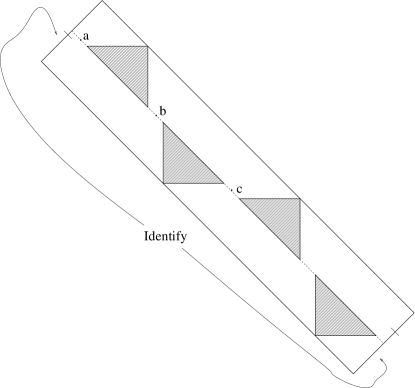
Figure 4: An illustration of the problems with constructing causality on $\bar{M}$. The spacetime is the interior of the rectangle, with the edges marked identified and the triangular regions removed; this spacetime is strongly causal. If we define a causality on $\bar{M}$ by $\bar{P}\prec_{I}\bar{Q}$ if $P\prec_{IP}Q$ or $P^{*}\prec_{IF}Q^{*}$, it will not give a partial ordering; $c\prec_{I}b$ and $b\prec_{I}a$, but $c\nprec_{I}a$. If we add additional causal relations to make a partial ordering, we will have $c\prec_{I}a$ and $a\prec_{I}c$, and the dashed line will be a closed causal curve. However, one may also choose to introduce the causality defined by the chronology in (12) so that $c\nprec_{C}b$. Thus, if one is willing to pay the price of losing the causal link between $b$ and $c$, one can eliminate closed causal curves in $\bar{M}$.

Alternatively, we can define the causality from the chronology. Since $\ll_{C}$ is a weakly distinguishing chronology, it determines a causality (see [13] for the proof). That is, one may define

$$\bar{P}\prec_{C}\bar{Q}\quad\mbox{iff }I^{-}_{C}(\bar{P})\subset I^{-}_{C}(\bar{Q})\mbox{ and }I^{+}_{C}(\bar{P})\supset I^{+}_{C}(\bar{Q}).$$ (12)

The causality $\prec_{C}$ satisfies conditions 5 and 6 of definition 5, and hence $\bar{M}$ with chronology $\ll_{C}$ and causality $\prec_{C}$ is a causal space (essentially by construction). In [8], this causality was briefly described and shown to define a causally simple $\bar{M}_{id}$. Thus, from a formal point of view, this causality is much better behaved than $\prec_{I}$. Note that $\bar{P}\prec_{C}\bar{Q}$ implies $\bar{P}\prec_{I}\bar{Q}$, the converses are not generally true; for example, in figure 4, $c\prec_{I}b$, but $c\nprec_{C}b$.

However, in practice, this causality fails to give the expected causal relations in some simple examples. Again we refer to figure 4, where one would expect $c\prec b$, but one finds $c\nprec_{C}b$. Another example, discussed in [4], shows that $\prec_{C}$ yields unexpected results even for causally continuous spaces.

Our approach to this issue is to admit to a certain ambivalence with respect to causality. Our feeling is that physical effects connected with signal propagation are related to the chronology $I^{\pm}_{C}(\bar{P})$ and perhaps to the closure of such sets. This closure is determined by the topology, which will be discussed in section 4 below, but again figure 4 shows that such relations are unlikely to lead to a causality. Thus, any desire to impose a causality on $\bar{M}$ must stem from other motivations that may vary with the precise context. If one insists on making $\bar{M}$ a causal space, one can do so using $\prec_{C}$. If, on the other hand, one finds it useful to encode apparent null relations such as those linking $a,b,c$ in figure 4, one may use $\prec_{I}$. In general, however, it is not possible to do both.

4 Topology on $\bar{M}$

The causal structure discussed in the previous section yields some information about the relation between the causal boundary and points in the interior. However, to provide a more complete description, we need to make $\bar{M}$ into a topological space. In the quotient constructions, the topology on $\bar{M}$ has played a central role in determining appropriate identifications to form the quotients, and it has been natural to construct the topology by the quotient of some suitable topology on the space of all IPs and IFs.

In this section, we will propose a new definition for the topology on the completion $\bar{M}$ we defined in section 2.3. We must construct our topology directly on $\bar{M}$. Following the philosophy of the previous sections, it is directly based on the causal structure of $\bar{M}$. In section 4.1, we will show that with this topology, the map $M\to\bar{M}$ is an open dense embedding, so $\bar{M}$ does correspond to $M$ equipped with boundary points in a suitable topological sense. In section 4.2, we consider the separation properties of our topology. As in [2], we will often omit dual results, obtained by exchanging future and past.

However, our definition of the topology will be fairly technical, and it is interesting to explore to what extent its features depend on the particular choices made in the definition. We therefore define a contrasting topology ${\bar{\cal T}}_{alt}$ by making slightly different technical choices in appendix B. We find that this alternative shares many features with our main definition of the topology, but has non-trivial differences in the treatment of some limits and in its separation properties. Both definitions suffer from (to some extent complementary) disadvantages, so we do not regard our work as completely settling the issue of the topology. It does however provide two data points which provide partial solutions, illustrate many of the relevant issues, and may be useful for future investigations.

Let us begin by reviewing previous work on the topology; although we cannot use it directly, it is an important source of inspiration for our definitions. In [2], a topology was first introduced on the set $M^{\sharp}$ defined in (1), and identifications were then imposed to define a set $\bar{M}_{id}$ which was Hausdorff in the induced topology. The topology on $M^{\sharp}$ was defined to be the coarsest topology such that for each $A\in\check{M}$, $B\in\hat{M}$, all the sets $A^{\rm int}$, $A^{\rm ext}$, $B^{\rm int}$ and $B^{\rm ext}$ are open, where

$$A^{\rm int}=\{P^{\sharp}:P\in\hat{M}\mbox{ and }P\cap A\neq\emptyset\},$$ (13)

$$A^{\rm ext}=\{P^{\sharp}:P\in\hat{M}\mbox{ and }\forall S\subset M,P=I^{-}[S]\Rightarrow\mbox{ not }I^{+}[S]\subset A\},$$ (14)

with $B^{\rm int}$ and $B^{\rm ext}$ defined similarly. These sets are meant to correspond roughly to $I^{-}(A^{\sharp})$, $M^{\sharp}\setminus J^{-}(A^{\sharp})$, $I^{+}(B^{\sharp})$, and $M^{\sharp}\setminus J^{+}(B^{\sharp})$ respectively. Thus, this topology is meant to correspond to a generalised Alexandrov topology; the additional open sets defined by the complement of the causal pasts and futures are necessary to construct suitable open neighbourhoods of TIPs and TIFs, as explained in [2].

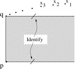
Figure 5: A spacetime introduced in [2] for which the causal completion can be defined to have at most two of the following three properties: i) causality, ii) Hausdorff topology, iii) the convergence of $x_{n}$ to $p$ and $q$. The shaded region is removed from two-dimensional flat space, and edges indicated identified. If the sequence $x_{n}$ has either $p$ or $q$ as a limit point, it must have both in any topology that does not distinguish past from future. In our causal construction, $p$ and $q$ are not identified. In the topology of definition 7, $\bar{M}$ is causal but neither of the other two properties hold. We introduce a contrasting topology in appendix B in which $x_{n}\rightarrow p,q$ and $\bar{M}$ is causal but not Hausdorff.

Although [8] uses the causal identification rule discussed previously, the topology on $\bar{M}_{id}$ is still obtained from the above topology on $M^{\sharp}$. Various problems with this topology have been discussed in the literature [3, 4, 6]. In particular, in [6], an example was constructed where certain sequences of points in $M$ do not have the expected limit points in $\bar{M}_{id}$. We will discuss a directly analogous example in the context of plane waves in section 5. An attempt to improve the GKP topology was made in [5], but it was also found to have difficulties [6].

In [7], by contrast, the topology is defined directly on $\bar{M}$. The topology defined in [7] is a generalised Alexandrov topology determined by the causal structures introduced on $\bar{M}$. That is, the sets $A^{\rm int}$, $A^{\rm ext}$, $B^{\rm int}$ and $B^{\rm ext}$ used in the GKP topology are replaced by the $I^{-}(\bar{A})$, $\bar{M}\setminus J^{-}(\bar{A})$, $I^{+}(\bar{B})$, $\bar{M}\setminus J^{+}(\bar{B})$ defined for elements $\bar{A},\bar{B}\in\bar{M}$ by a suitable chronology and causality relations on $\bar{M}$. We will not discuss these relations in detail as they were intended to apply only to causally continuous spaces.

Let us now turn to the construction of a topology on our $\bar{M}$. Since our whole approach centres around the definition of a chronology $\ll_{C}$ on $\bar{M}$, the most natural topology is an Alexandrov topology, where the chronological future- and past-sets $I^{\pm}_{C}(\bar{Q})$ form a subbasis. However, as argued in [2], this is not a sufficiently strong topology; it does not provide suitable open neighbourhoods for all ideal points. One might consider extending it by introducing a generalised Alexandrov topology using both the chronology and the causality, as in [7]. This avenue is obstructed by the absence of a truly satisfactory causality in $\bar{M}$ for general strongly causal $M$. The only candidate in general is $\prec_{C}$; but in figure 4, $c\nprec b$, so $b\in\bar{M}\setminus J^{+}_{C}(c)$, and $[\bar{M}\setminus J^{+}_{C}(c)]\cap M$ is not an open set in the manifold topology on $M$. That is, $M$ is not homeomorphic to its image in $\bar{M}$ with such a topology, so this topology is not generally satisfactory.

We therefore need to adopt a more indirect route in the definition of our topology. However, we will see in Lemma 3 below that the topology we define will contain the Alexandrov topology; that is, all the chronological future- and past-sets $I^{\pm}_{C}(\bar{Q})$ are open in our topology. The topology we adopt is based on defining suitable closed sets, in a modified version of the other part of the GKP topology. We want to use the chronology to define sets $L^{\pm}(\bar{S})$ for any subset $\bar{S}\subset\bar{M}$, such that we can define a reasonable topology by requiring $\bar{M}\setminus L^{\pm}(\bar{S})$ to be open. We start by defining the sets

$$L^{+}_{IF}(\bar{S})=\{\bar{Q}\in\bar{M}:Q^{*}\neq\emptyset,Q^{*}\subset\cup_{\bar{P}\in\bar{S}}P^{*}\},$$ (15)

$$L^{-}_{IP}(\bar{S})=\{\bar{Q}\in\bar{M}:Q\neq\emptyset,Q\subset\cup_{\bar{P}\in\bar{S}}P\}.$$ (16)

Note that for $p\in M$, $p\in\bar{S}$ implies $p\in L^{+}_{IF}(\bar{S})$ and $p\in L^{-}_{IP}(\bar{S})$, as $I^{+}(p)\subset\cup_{\bar{P}\in\bar{S}}P^{*}$ and $I^{-}(p)\subset\cup_{\bar{P}\in\bar{S}}P$. If we applied these definitions to a manifold, they would give $Cl[I^{\pm}(\bar{S})]$, so this seems a natural way to define closed sets from the causality. However, as they stand, these cannot in general be good closed sets in $\bar{M}$, because they only contain IFs (respectively, IPs), and so can never contain TIPs (TIFs) corresponding to future (past) boundary points. To rectify this, we introduce operations $Cl_{FB}$ and $Cl_{PB}$, the closures in the future and past boundaries, by

$$Cl_{FB}(\bar{S})=\bar{S}\cup\{\bar{Q}\in\bar{M}:Q^{*}=\emptyset,Q=\lim\ P_{n}\ {\rm for}\ \{P_{n}\}\in\bar{S}\},$$ (17)

$$Cl_{PB}(\bar{S})=\bar{S}\cup\{\bar{Q}\in\bar{M}:Q=\emptyset,Q^{*}=\lim\ P_{n}^{*}\ {\rm for}\ \{P^{*}_{n}\}\in\bar{S}\},$$ (18)

where the limit of a sequence of past sets $\{P_{n}\}$ is given by

Definition 6

$Q=\lim\ P_{n}$ if and only if

1. For each $x\in Q$, there is some $N$ such that $x\in P_{n}$ for all $n>N$.

2. For each $x$ such that $I^{-}(x)\not\subset Q$, there is some $N$ such that $I^{-}(x)\not\subset P_{n}$ for all $n>N$.

The limit of a sequence of future sets is defined similarly. There are, of course, many sequences $\{P_{n}\}$ which do not converge and for which no such limit exists. Since $M$ is a strongly causal spacetime, a lemma below (lemma 2) will show that (ii) is equivalent to:

ii) For each $x\notin Cl[Q]$, there is some $N$ such that $x\notin Cl[P_{n}]$ for all $n>N$.

However, we prefer the first definition above which is more directly associated with the causal structure.

These operations add only future (past) boundary points to $\bar{S}$ (as the subscripts suggest), and as an immediate consequence $Cl_{FB,PB}(\bar{S})\cap M=\bar{S}\cap M$. We then define sets

$$L^{+}(\bar{S})=Cl_{FB}[\bar{S}\cup L^{+}_{IF}(\bar{S})],$$ (19)

$$L^{-}(\bar{S})=Cl_{PB}[\bar{S}\cup L^{-}_{IP}(\bar{S})].$$ (20)

Note also that $L^{\pm}$ are not necessarily symmetric; $p\in L^{\pm}(q)$ does not imply $q\in L^{\mp}(p)$. For example, in figure 4, $b\in L^{-}(a)$, but $a\notin L^{+}(b)$. This implies $L^{\pm}$ are also not related to the causal future and past in any causality on $\bar{M}$. On the other hand, we have $L^{+}(\bar{S})\cap M=L^{+}_{IF}(\bar{S})\cap M$, $L^{-}(\bar{S})\cap M=L^{-}_{IP}(\bar{S})\cap M$, so these definitions are just adding some boundary points to make $L^{\pm}_{IF,IP}$ look more like closed sets.

We can now define our topology:

Definition 7

The topology $\bar{\cal T}$ on $\bar{M}$ is defined to be the coarsest in which all the sets $\bar{M}\setminus L^{\pm}(\bar{S})$ are open for any $\bar{S}\subset\bar{M}$.

Note that the above is equivalent to stating that the collection of $\bar{M}\setminus L^{\pm}(\bar{S})$ form a sub-basis for the topology, as the definition amounts to saying that all those sets and only those sets which can be written as arbitrary unions and finite intersections of the sets $\bar{M}\setminus L^{\pm}(\bar{S})$ are open.

4.1 $\bar{M}$ is $M$ with a boundary

Our first task is to understand the relation of this topology to the manifold topology on $M$. We will show that the natural map $\Phi:M\to\bar{M}$ is a homeomorphism from $M$ to $\Phi(M)$, and that the image $\Phi(M)$ is dense in $\bar{M}$. This shows that with our topology $\bar{\cal T}$, the completion $\bar{M}$ does equip $M$ with a boundary in a topological sense. Thus, our topology satisfies the main requirement we argued for in the introduction; it enables us to use $\bar{M}$ as a tool for discussing limits in $M$.

It is useful to introduce the notion of a future-closed set:

Definition 8

A set $S\subset M$ is future-closed in $M$ if and only if $\forall x\in S$, $I^{+}(x)\subset S$.

We define past-closed sets in $M$ and future- and past-closed sets in $\bar{M}$ similarly. Note that a future-set is always future-closed. Note that $L^{+}(\bar{S})\cap M$ is future-closed in $M$ and $L^{+}(\bar{S})$ is future-closed in $\bar{M}$. We now prove some useful lemmas (we omit dual results, where future and past are exchanged).

Lemma 1

For a future-closed set $F\subset M$, every point in the boundary of $F$ (in $M$, using the topology of $M$) can be approached from the future along some curve $\gamma\subset F$.

Proof: Since $M$ is strongly causal, every $x$ in the boundary of $F$ has an open neighborhood $U$ which is both homeomorphic and causally isomorphic to an Alexandrov neighborhood in Minkowski space. This implies $I^{+}(x)\cap U\subset F$, and $x$ can be approached from the future along $\gamma\subset I^{+}(x)\cap U\subset F$. $\Box$

Lemma 2

Given $\bar{S}\subset\bar{M}$, $L^{+}(\bar{S})\cap M$ is a closed subset of $M$.

Proof: Since $L^{+}(\bar{S})\cap M=L^{+}_{IF}(\bar{S})\cap M$ is a future-closed set, any point $y$ in its boundary (in $M$) can be approached from the future along a timelike curve $\gamma\subset L^{+}(\bar{S})\cap M$. As a result, $y$ has $I^{+}(y)=I^{+}[\gamma]\subset\cup_{\bar{Q}\in\bar{S}}Q^{*}$ and so $y\in L^{+}_{IF}(\bar{S})$. $\Box$

Lemma 3

The sets $I^{\pm}_{C}(\bar{S})$ are open in $\bar{M}$ for every $\bar{S}\subset\bar{M}$.

Proof: To show this, we will prove $I^{+}_{C}(\bar{S})=\bar{M}\setminus L^{-}(\bar{S}^{+})$ for suitable $\bar{S}^{+}$. Let

$$\bar{S}^{+}=\bar{M}\setminus I^{+}_{C}(\bar{S}).$$ (21)

Then since $L^{-}(\bar{S}^{+})\supset\bar{S}^{+}=\bar{M}\setminus I^{+}_{C}(\bar{S}),$ it is clear that $I^{+}_{C}(\bar{S})\supset\bar{M}\setminus L^{-}(\bar{S}^{+})$.

Thus, we need only show $I^{+}_{C}(\bar{S})\subset\bar{M}\setminus L^{-}(\bar{S}^{+})$, which is equivalent to $I^{+}_{C}(\bar{S})\cap L^{-}(\bar{S}^{+})=\emptyset$. Now $I^{+}_{C}(\bar{S})\cap L^{-}(\bar{S}^{+})=I^{+}_{C}(\bar{S})\cap L^{-}_{IP}(\bar{S}^{+})$, as no past boundary point can belong to $I^{+}_{C}(\bar{S})$, and $I^{+}_{C}(\bar{S})\cap\bar{S}^{+}=\emptyset$ by definition. Furthermore, the definition of $\bar{S}^{+}$ is equivalent to

$$\bar{S}^{+}=\{\bar{P}:P\cap R^{*}=\emptyset\ \forall\bar{R}\in\bar{S}\}.$$ (22)

Hence $(\cup_{\bar{P}\in\bar{S}^{+}}P)\cap R^{*}=\emptyset$ for all $\bar{R}\in\bar{S}$. Any point $\bar{Q}\in L^{-}_{IP}(\bar{S}^{+})$ has $Q\subset\cup_{\bar{P}\in\bar{S}^{+}}P$, so $Q\cap R^{*}=\emptyset$ for all $\bar{R}\in\bar{S}$. Thus, $I^{+}_{C}(\bar{S})\cap L^{-}(\bar{S}^{+})=I^{+}_{C}(\bar{S})\cap L^{-}_{IP}(\bar{S}^{+})=\emptyset$. We conclude that,

$$I^{+}_{C}(\bar{S})\subset[\bar{M}\setminus L^{-}(\bar{S}^{+})].$$ (23)

$\Box$

We may now prove one of the crucial theorems in our work.

Theorem 5

$M$ is homeomorphic to its image in $\bar{M}$.

Proof: By lemma 2 above (and the obvious dual) the sets $L^{\pm}(\bar{S})\cap M$ are closed sets in the topology of $M$. Thus, the open sets of the induced topology are open sets in the manifold topology on $M$.

It remains to show that we include all the open sets in the manifold topology. But from theorem 3 we have the equality $I^{\pm}(p)=I^{\pm}_{C}(p)\cap M$. By lemma 3 these sets are open in the topology induced on $M$ from $\bar{M}$. Since $M$ is strongly causal, these sets form a subbasis for the manifold topology and any open set $U\subset M$ is of the form $\bar{U}\cap M$ for some $\bar{U}$ open in $\bar{M}$. $\Box$

This theorem shows that the topology we are defining is compatible with the pre-existing topology on $M$, in much the same way that we saw that the chronology on $\bar{M}$ was compatible with the pre-existing chronology on $M$ in section 3.1. In fact, we can do slightly better:

Theorem 6

Any subset $U\subset M$ is open if and only if $\Phi(U)\subset\bar{M}$ is open in $\bar{M}$.

Proof: Choose $x,y\in M$ such that $I^{+}(x)\cap I^{-}(y)$ lies in a set $K\subset M$ which is compact in the manifold topology. Consider $\bar{P}\in I^{+}_{C}(x)\cap I^{-}_{C}(y)$. Then $\bar{P}$ is attached by timelike curves through $M$ to $x$ and $y$. Thus, either $\bar{P}\in M$ or $\bar{P}$ is a TIP of some curve $\gamma$ (and also a TIF of some $\gamma^{\prime}$) in $I^{+}(x)\cap I^{-}(y)$. But since $I^{+}(x)\cap I^{-}(y)$ lies within a compact set in $M$, there are no such TIPs or TIFs and $I^{+}_{C}(x)\cap I^{-}_{C}(y)=I^{+}(x)\cap I^{-}(y)$. Such sets are open in $\bar{M}$ by lemma 3. Finally, since any open set in $M$ is the union of such Alexandrov sets, it is open in $\bar{M}$.

On the other hand, if $\Phi(U)$ is open in $\bar{M}$, $U$ is open in $M$ by theorem 5. $\Box$

4.1.1 Limits in $\bar{M}$

The main purpose in introducing a topology is that it allows us to give some sequences in $M$ ideal points as endpoints. Thus, we can discuss asymptotic behaviour in $M$ in terms of the points of $\bar{M}$. We would now like to show that the limits defined by the topology introduced above are consistent with the chronology. That is, we would like to see that ideal points which are limit points in a casual sense are also limit points in a topological sense.

Lemma 4

For $x\in L^{+}(\bar{S})$ and any timelike curve $\gamma$ through $x$, we have $\bar{Q}\in L^{+}(\bar{S})$ for any point of the form $\bar{Q}=(I^{-}[\gamma],Q^{*})\in\bar{M}$.

Proof: We have $Q^{*}\subset f(I^{-}[\gamma])\subset I^{+}(x)\subset\cup_{\bar{P}\in\bar{S}}P^{*}$, so $I^{-}[\gamma]\in L^{+}(\bar{S})$, unless $Q^{*}=\emptyset$. In the latter case, consider a sequence of points $x_{n}\in\gamma$ such that $\lim\ I^{-}(x_{n})=I^{-}[\gamma]$. By the above argument, $x_{n}\in L^{+}_{IP}(\bar{S})$, so $\bar{Q}\in Cl_{FB}[\bar{S}\cup L^{+}_{IP}(\bar{S})]=L^{+}(\bar{S})$. $\Box$

Theorem 7

For a timelike curve $\gamma$, any $\bar{P}\in\bar{M}$ of the form $\bar{P}=(I^{-}[\gamma],P^{*})$ is a future endpoint of $\gamma$ in $\bar{M}$.

Proof: Since we have already shown that $M$ is homeomorphic to its image in $\bar{M}$, the case where $I^{-}[\gamma]$ is a PIP is trivial. Thus we suppose it is a TIP. Parametrize the curve $\gamma$ by $\lambda$ increasing towards the future. We wish to prove that any open set $U\subset\bar{M}$ (in our topology above) containing $\bar{P}$ also contains a future segment of $\gamma$—that is, it contains $x(\lambda)$ for $\lambda>\lambda_{c}$ for some $\lambda_{c}$. It is sufficient to prove this for the subbasis that generates the topology, so we may take $U=\bar{M}\setminus L^{\pm}(\bar{S})$.

So, suppose $\bar{P}\notin L^{-}(\bar{S})$, which implies $\bar{P}\notin L^{-}_{IP}(\bar{S})$, since $P=I^{-}[\gamma]$ is an IP. Then $I^{-}[\gamma]$ is not a subset of $\cup_{\bar{Q}\in\bar{S}}Q$. But $I^{-}[\gamma]$ is the union of $I^{-}(x)$ for $x\in\gamma$ and the $I^{-}(x)$ form an increasing sequence. Thus, there must be some $\lambda_{c}$ such that $I^{-}[x(\lambda_{c})]$ is not a subset of $\cup_{\bar{Q}\in\bar{S}}Q$. As a result, $x(\lambda_{c})\notin L^{-}(\bar{S})$. Furthermore, since $I^{-}[x(\lambda_{1})]\subset I^{-}[x(\lambda_{2})]$ for $\lambda_{1}<\lambda_{2}$, $x(\lambda)\notin L^{-}(\bar{S})\forall\lambda>\lambda_{c}$. Thus $\bar{M}\setminus L^{-}(\bar{S})$ contains $x(\lambda)$ for all $\lambda>\lambda_{c}$.

Now suppose $x\in L^{+}(\bar{S})$ for some $x\in\gamma$. Then from lemma 4 $\bar{P}\in L^{+}(\bar{S})$. Thus, $\bar{P}\in\bar{M}\setminus L^{+}(\bar{S})$ implies $x\in\bar{M}\setminus L^{+}(\bar{S})$ for all $x\in\gamma$. $\Box$

This theorem shows that this topology satisfies a minimal criterion for consistency with the causal structure. An immediate corollary of this result is that $M$ is a dense subset of $\bar{M}$, since every open neighbourhood of a TIP $I^{-}[\gamma]$ contains points of $M$, namely the future segment of $\gamma$. Thus, $\bar{M}$ is $M$ with a boundary.

A more general relation between causal and topological limits can in fact be proved, using the notion of limits introduced in definition 6:

Theorem 8

If $P=\lim\ I^{-}(x_{n})$ and $P^{*}=\lim\ I^{+}(x_{n})$ for some $\bar{P}=(P,P^{*})\in\bar{M}$, the sequence $\{x_{n}\}\subset M$ converges to $\bar{P}$ in the topology on $\bar{M}$.

Proof: We need to show that the sequence $\{x_{n}\}$ enters every open neighbourhood of $\bar{P}$. As in the proof of theorem 7, it is sufficient to consider the subbasis $\bar{M}\setminus L^{\pm}(\bar{S})$. Equivalently, we wish to show that $x_{n}\in L^{\pm}(\bar{S})$ for $n>N$ for some $N$ implies $\bar{P}\in L^{\pm}(\bar{S})$.

Now $x_{n}$ is an ordinary point, so $x_{n}\in L^{-}(\bar{S})$ implies $I^{-}(x_{n})\subset\cup_{\bar{Q}\in\bar{S}}Q$. If $P$ is non-empty, $P=\lim\ I^{-}(x_{n})$ implies that every $x\in P$ is in $I^{-}(x_{n})$ for $n>N$; hence $x\in\cup_{\bar{Q}\in\bar{S}}Q$ for every $x\in P$. That is, $P\subset\cup_{\bar{Q}\in\bar{S}}Q$, and hence $\bar{P}\in L^{-}(\bar{S})$. If on the other hand $P$ is empty, $x_{n}\in L^{-}_{IF}(\bar{S})$ and $P^{*}=\lim\ I^{+}(x_{n})$ implies $\bar{P}$ is in $Cl_{PB}[L^{-}_{IF}(\bar{S})]$, and so $\bar{P}\in L^{-}(\bar{S})$. The dual proof for futures is the same. $\Box$

In our approach, based on IP-IF pairs, these two theorems seem like an appropriate statement of the consistency between topological and causal limits. Like our definition of $\bar{M}$, theorem 8 uses the information in both pasts and futures. There is an obvious weaker version of the statement of theorem 8, which would require that $\{x_{n}\}$ converges to $\bar{P}$ if $P=\lim\ I^{-}(x_{n})$ or $P^{*}=\lim\ I^{+}(x_{n})$. There is no reason to expect this to be generally satisfied. Indeed, figure 6 provides an example where $P=\lim\ I^{-}(x_{n})$ but we do not want the topology to be such that the $\{x_{n}\}$ converge to $\bar{P}$. Indeed, they do not in our topology above, though they do converge to both $\bar{P}$ and $\bar{Q}$ in the topology $\bar{\cal T}_{alt}$ introduced in appendix B. Returning to the topology $\bar{\cal T}$, since theorem 7 (and the obvious dual) makes reference only to pasts or futures, this weaker form will in fact be satisfied in some cases. For example, in figure 3, any curve such that $A=I^{-}[\gamma]$ has both $(A,B^{*})$ and $(A,C^{*})$ as limit points, even though $I^{+}(x_{n})\to B^{*}\cup C^{*}$ along $\gamma$.

Figure 6: An example where $P=\lim\ I^{-}(x_{n})$ but we do not expect the $\{x_{n}\}$ converge to $\bar{P}$. Rather, the $\{x_{n}\}$ intuitively converge to a point at ‘spacelike infinity’ which is not included in the causal completion $\bar{M}$. It is interesting to note that although a point at spacelike infinity cannot have any spacetime regions to its future or past, this does not imply that sequences $\{x_{n}\}$ which go to spacelike infinity have $\lim\ I^{\pm}(x_{n})=\emptyset$.

However, while the topology is thus consistent with the causality, it may not give all the limits we would intuitively expect. For example, in figure 5, the pasts of the $x_{n}$ will approach the past of $q$, while the futures will approach the future of $p$. Hence, the sequence $\{x_{n}\}$ is not guaranteed to converge to either $p$ or $q$. In fact, $q\notin L^{+}(\{x_{n}\})$ and $p\notin L^{-}(\{x_{n}\})$, so $\bar{M}\setminus L^{\pm}(\{x_{n}\})$ are open sets containing $q$ ($p$) which the sequence never enters, and hence the sequence $\{x_{n}\}$ converges to neither of the points, whereas we would intuitively expect it to converge to both. The same would be true if the $\{x_{n}\}$ were arrayed along a null line from $p$ or $q$. Now one could take the attitude that our intuition is using additional information that is not contained in the causal structure in this case; our argument above suggests that the causal structure alone does not allow us to unequivocally say that this sequence should or should not converge. However, there are some somewhat arbitrary choices in our definition of the topology; in appendix B, we explore a slightly different alternative definition of the topology which produces the more intuitively satisfying answer in this example.

4.2 Separation properties of $\bar{M}$

Having seen that the topology $\bar{\cal T}$ is compatible with the manifold topology on $M$, we would like to investigate its separation properties. We have previously argued that we should not assume that the topology will be Hausdorff in general. Szabados has argued in [8, 9] that compatibility with the definition of the boundary from the causal structure suggests that we impose a slightly weaker separation condition, dubbed $T_{c}$, which asserts that every causal curve has a unique endpoint in $\bar{M}$. However, in figure 3, the points $(A,B^{*})$ and $(A,C^{*})$ are both future endpoints of the same causal curve, so $T_{c}$ (and hence also Hausdorffness) must fail. Hence, in our approach where $\bar{M}$ is constructed from IP-IF pairs, assuming $(\bar{M},\bar{\cal T})$ is Hausdorff or $T_{c}$ would be incompatible with demanding that the topological notion of limits is consistent with the causal notion.

Figure 7: An example in which $\bar{M}$ is not $T_{1}$. Every closed set containing $\bar{P}=(I^{-}[\gamma],P^{*})$ also contains $\bar{P}^{\prime}=(I^{-}[\gamma^{\prime}],\emptyset)$.

While our topology will not satisfy Szabados’ $T_{c}$ condition in its original form, his arguments suggest that we should demand that the only future endpoints of a curve $\gamma$ in $\bar{M}$ are the points of the form $(I^{-}[\gamma],P_{i}^{*})$. Unfortunately, this is again false in our topology. In fact, even more worryingly, in general it does not even satisfy the $T_{1}$ condition (which states that for any two points $\bar{P},\bar{Q}\in\bar{M}$, there are open sets ${\cal O}_{P},{\cal O}_{Q}\in\bar{\cal T}$ containing $\bar{P}$ but not $\bar{Q}$ and vice-versa). Figure 7 shows an example in which every closed set containing $\bar{P}$ also contains $\bar{P}^{\prime}$, and thus every open set containing $\bar{P}^{\prime}$ contains $\bar{P}$. The example comes from figure 3 of [9]. In this example, an infinite set of null lines (including the limit point $r$) have been removed from Minkowski space in such a way that future-directed timelike curves may cross from left to right but not from right to left. Thus, there are two interesting TIPs, $P^{\prime}=I^{-}[\gamma^{\prime}]$, $P=I^{-}[\gamma]$, with $P^{\prime}\subset P$. Note that there is a pair $\bar{P}=(P,P^{*})$ in $R_{pf}$, but not $(P^{\prime},P^{*})$, since $P^{\prime}\subset P$ is not maximal in any $p(P^{*})$; rather, we have $\bar{P}^{\prime}=(P^{\prime},\emptyset)\in\bar{M}$. One can easily see that $\bar{P}^{\prime}\in L^{-}(\bar{P})$. In addition, $\bar{P}^{\prime}\in L^{+}(p)$ for any $p\in P$, since $I^{-}(q_{n})$ converge to $P^{\prime}$. Thus, $\bar{P}^{\prime}$ lies in any closed set containing $\bar{P}$, and $\bar{P}$ lies in any open set containing $\bar{P}^{\prime}$.

This example shows that we cannot hope to prove that the causal completion $\bar{M}$ with the topology introduced above satisfies even the $T_{1}$ separation axiom in general. Our course in the remainder of this section will first be to prove what we can, seeing how far we can get with partial results which serve to isolate the problems with the topology somewhat, and then discuss what we should do about them.

It follows immediately from theorem 6 that any two points $p,q\in M$ are $T_{2}$ separated in $\bar{M}$. We can prove that any point $x\in M$ is $T_{2}$ separated from any ideal point by a series of theorems:

Theorem 9

Any point $p$ in a causal curve $\gamma$ is $T_{2}$ separated from any point of the form $\bar{P}=(I^{-}[\gamma],P^{*})\in\bar{M}$.

Proof: To find an open set containing $p$ but not $I^{-}[\gamma]$, use Theorem 6 to choose any open $U\subset M$ containing $p$. For later convenience, take $U\subset I^{-}(q)$ for some $q\in\gamma$ with $I^{-}(q)\supset I^{-}(p)$.

On the other hand, to find an open set containing $I^{-}[\gamma]$ but not $p$, consider $\bar{M}\setminus L^{-}(q)$ for the same $q$ used above. Clearly $p\in L^{-}(q)$, so $p\notin\bar{M}\setminus L^{-}(q)$. Note that $q\notin I^{-}(q)$ since $M$ is causal. Thus, $I^{-}(\gamma)\not\subset I^{-}(q)$ and $\bar{P}\notin L^{-}_{IF}(q)$. But since $I^{-}[\gamma]$ is a nonempty IP, $\bar{P}$ does not lie on the past boundary and we also have $\bar{P}\in\bar{M}\setminus L^{-}(q)$.

Since $I^{-}(q)\cap[\bar{M}\setminus L^{-}(q)]=\emptyset$ we have shown that $p$ and $\bar{P}$ are $T_{2}$ separated. $\Box$

Theorem 10

If $K\subset M$ is compact in $M$, then $\Phi(K)$ is closed in $\bar{M}$.

Proof: For each TIP $P$, choose some timelike curve $\gamma$ which generates $P$ (i.e., with $P=I^{-}[\gamma]$) and choose some $x\in\gamma$ such that $I^{+}(x)\cap K=\emptyset$ (this is possible by strong causality). Recall that $I^{+}_{C}(x)$ is open in $\bar{M}$ by lemma 3, and that this set contains any $\bar{P}=(I^{-}[\gamma],P^{*})\in\bar{M}$. Taking the union of such sets creates an open set which contains all TIPs but which does not intersect $K$. We can similarly construct an open set which contains all TIFs and does not intersect $K$. Finally, from theorem 6 and the Hausdorff property of $M$, given any $y\in M\setminus K$, we can find $U_{y}\ni y$ open in $\bar{M}$ for which $U_{y}\cap K=\emptyset$. The union of all such sets must be open, and is clearly $\bar{M}\setminus\Phi(K)$. Thus, $\Phi(K)$ is closed in $\bar{M}$. $\Box$

An immediate corollary of this theorem is that any point $p\in M$ is $T_{2}$ separated from any ideal point $\bar{P}$: we may choose any $K\ni x$ compact in $M$ and any open $U\subset K$ containing $x$. Then $\bar{M}\setminus\Phi(K)$ is an open set containing $\bar{P}$ but not $x$, while $U$ contains $x$ but not $\bar{P}$, and $U\cap\bar{M}\setminus\Phi(K)=\emptyset$.

Thus, points $p\in M$ are $T_{2}$ separated from each other and from ideal points. It remains to consider the separation of ideal points among themselves. First, consider the ideal points which are future endpoints of the same timelike curve $\gamma$ in the causal sense.

Theorem 11

For any timelike curve $\gamma$, all the ideal points $\bar{P}_{i}$ with $P_{i}=I^{-}[\gamma]$ are $T_{1}$ separated.

Proof: We must have $P^{*}_{i}\subset f(I^{-}[\gamma])$ for each $i$, and furthermore we cannot have $P^{*}_{i}\subset P^{*}_{j}$ for $i\neq j$, or $P^{*}_{i}$ would not be maximal. Thus, $\bar{P}_{i}\notin L^{+}(\bar{P}_{j})$ for $i\neq j$. Hence $\bar{M}\setminus L^{+}(\bar{P}_{j})$ is an open set containing $\bar{P}_{i}$ but not $\bar{P}_{j}$. $\Box$

Hence, the failure of $T_{1}$ is not associated with our decision to ascribe several future endpoints to the same curve in some cases.

Let us consider the more general case, not covered by this proof. There are four different cases (omitting those which just swap $\bar{P}$ and $\bar{Q}$ or pasts and futures): 1. Both $P$ and $P^{*}$ nonempty, both $Q$ and $Q^{*}$ nonempty; 2. Both $P$ and $P^{*}$ nonempty, $Q^{*}=\emptyset$; 3. $P^{*}=\emptyset$, $Q^{*}=\emptyset$; 4. $P^{*}=\emptyset$, $Q=\emptyset$.

Theorem 12

Consider points $\bar{P}\neq\bar{Q}$ in $\bar{M}$.

1. If both $P$ and $P^{*}$ are nonempty and both $Q$ and $Q^{*}$ are nonempty, $P\neq Q$, $P^{*}\neq Q^{*}$, the two points are $T_{c}$ (and thus $T_{1}$) separated.

2. If both $P$ and $P^{*}$ are nonempty but $Q^{*}=\emptyset$, the two points are $T_{0}$ separated.

3. If $P^{*}=\emptyset$ and $Q^{*}=\emptyset$, the two points are $T_{1}$ separated.

4. If $P^{*}=\emptyset$ and $Q=\emptyset$, the two points are $T_{1}$ separated.

Proof:

1. For $T_{c}$ separation to fail, there must be some curve $\gamma$ such that $I^{-}[\gamma]=P$ and every open neighbourhood of $\bar{Q}$ contains a future segment of $\gamma$. This implies $\bar{Q}\notin\bar{M}\setminus L^{-}(\bar{P})$ and $\bar{Q}\notin\bar{M}\setminus L^{+}(x)$ for any point $x\in\gamma$, as $\gamma$ does not enter either of these sets towards the future. That is, to violate $T_{c}$, we must have $\bar{Q}\in L^{-}(\bar{P})$ and $\bar{Q}\in L^{+}(x)$ for all $x\in\gamma$, where $P=I^{-}[\gamma]$. Now $\bar{Q}\in L^{-}(\bar{P})$ implies $Q\subset I^{-}[\gamma]$, and $\bar{Q}\in L^{+}(x)$ implies $Q^{*}\subset I^{+}(x)$ for any $x\in\gamma$. This implies $p(I^{+}(x))\subset p(Q^{*})$, and as $I^{-}[\gamma]=\cup_{x\in\gamma}I^{-}(x)\subset\cup_{x\in\gamma}p(I^{+}(x))$, we have $Q\subset P\subset p(Q^{*})$, which contradicts the assumption that $(Q,Q^{*})\in R_{pf}$, since $P\neq Q$. Hence the points are $T_{c}$ (and thus $T_{1}$) separated.

2. $L^{+}(\bar{Q})=\bar{Q}$; hence $\bar{M}\setminus L^{-}(\bar{Q})$ contains $\bar{P}$ but not $\bar{Q}$, and the two points are $T_{0}$ separated. Note that for $T_{1}$ to fail, we must have $\bar{Q}\in L^{-}(\bar{P})$, so $Q\subset P$.

3. $L^{+}(\bar{P})=\bar{P}$; hence $\bar{M}\setminus L^{+}(\bar{P})$ contains $\bar{Q}$ but not $\bar{P}$. Similarly, $\bar{M}\setminus L^{+}(\bar{Q})$ contains $\bar{P}$ but not $\bar{Q}$. Hence the two points are $T_{1}$ separated.

4. $L^{+}(\bar{P})=\bar{P}$; hence $\bar{M}\setminus L^{+}(\bar{P})$ contains $\bar{Q}$ but not $\bar{P}$. Similarly, $\bar{M}\setminus L^{-}(\bar{Q})$ contains $\bar{P}$ but not $\bar{Q}$. Hence the two points are $T_{1}$ separated. $\Box$

There are two interesting points to this theorem. First of all, it shows that violations of $T_{1}$ happen only in cases which have the flavor of figure 7: there must be a pair of ideal points $\bar{P}$ and $\bar{Q}$ such that $Q^{*}=\emptyset$ and $Q\subset P$ (or dually $Q=\emptyset$ and $Q^{*}\subset P^{*}$). Thus, the conditions under which violations of $T_{1}$ can arise are restricted and reasonably well-understood. Furthermore, we see that all the ‘unexpected’ violations of $T_{c}$ (where $\bar{Q}$ is a future endpoint of a curve $\gamma$ for which $Q\neq I^{-}[\gamma]$) involve cases where at least one of the pasts and futures involved is empty. Hence, the points which fail to be appropriately separated would not have been identified even if we had adopted the quotient approach, completing $R_{pf}$ to the equivalence relation $\bar{R}_{pf}$.

Now we should consider what we want to do about the violations of $T_{1}$. In the example of figure 4, it was clear that preserving the causal structure was more important than ensuring a Hausdorff topology. The example of figure 7 is less clear, and one might consider it more natural to identify the two ideal points that fail to be $T_{1}$ separated.

Imposing such identifications in general will once again lead to problems with the chronology. One can construct an example where problems arise by introducing barriers of the kind indicated by the solid lines in figure 7 in both the past and the future of some point, in a somewhat more complicated version of the example in appendix A, containing even more regions. Thus, any identifications will have to be performed on a case by case basis. The question then is whether it is better to live with the completion $\bar{M}$, which is at least generally defined, even if some points are not $T_{1}$ separated, or to identify points as much as we can without introducing new chronological relations? If one does not want to impose any identifications, one has a further choice of approach. Either one regards $T_{1}$ separation as a desirable but not essential property, and works with this completion $\bar{M}$ for any strongly causal manifold, or one can insist that $T_{1}$ separation is important, and only accept the completion for those cases where the topology $\bar{\cal T}$ satisfies $T_{1}$. Note that the latter approach is closer to that adopted in [9], where the discussion was restricted to manifolds satisfying certain ‘asymptotic causality conditions’ in addition to strong causality. We will leave these issues for future discussion. In the unlikely event that such problematic cases are encountered in practical applications, the physics of the situation should provide better guidance than we can give here.

5 Homogeneous Plane Waves

Plane wave spacetimes [16, 17, 18, 19, 20, 21] provide a very interesting set of examples to which these techniques may be applied. The simplest non-trivial cases are smooth homogeneous plane waves. Except in two special cases which are conformally flat, the presence of a homogeneous Weyl tensor implies that these spacetimes cannot be conformally embedded into a compact region of a smooth manifold. Thus, the only available tool for discussing the asymptotic structure of these spacetimes is the causal boundary approach. Application of this technique was first considered in [11], where it was argued that for homogeneous plane waves satisfying any positive energy condition, the causal boundary generically consists of a single null line. This was in agreement with the results found in [15] for a conformally flat special case by conformally embedding the planewave in $S^{n}\times R$. See [22] for comments on how the generic behaviour differs from the conformally flat case when the behaviour of spacelike curves is considered. The causal boundary of plane waves has been further studied in [23].

We will now discuss the construction of the causal boundary for the plane wave using the approach we have introduced, showing that we recover the results of [11]. Homogeneous plane waves illustrate the differences between the various ways of constructing $\bar{M}$ in an interesting way, so we will also briefly compare the results to those of the previous quotient constructions. The results of [11] are also obtained when the Budic-Sachs-Szabados identifications are used; using the original GKP recipe for identifications, on the other hand, yields no identifications between TIPs and TIFs.

Figure 8: A 1+1 dimensional slice of the Einstein static universe along a great circle of the sphere. Left and right sides of the diagram are identified. The winding null ray indicates the conformal boundary of the conformally flat plane wave under the Berenstein-Nastase conformal embedding [15].

The class of smooth homogeneous plane waves considered in [11] is described by the metric

$$ds^{2}=-2dx^{+}dx^{-}-(\mu_{1}^{2}x_{1}^{2}+\ldots+\mu_{j}^{2}x_{j}^{2}-m_{1}^{2}y_{1}^{2}-\ldots-m_{n-j}^{2}y_{n-j}^{2})dx_{+}^{2}+dx^{i}dx^{i}+dy^{a}dy^{a},$$ (24)

where $\mu_{1}\geq\mu_{2}\geq\ldots\geq\mu_{j}$. We assume there is at least one $x^{i}$ (that is, $j\neq 0$), excluding a case with all negative directions which violates the positive energy conditions and has a different causal boundary. The special case $j=n$, $\mu_{1}=\mu_{2}=\ldots=\mu_{n}$ is conformally flat, and it was shown in [15] that this conformally flat plane wave can be embedded into the Einstein static universe, as depicted in figure 8. This conformal embedding into $S^{n}\times R$ maps this plane wave onto the entire space, save for a single null geodesic $N$.

In [11], the definitions of section 2.1 were applied to find that the TIPs and TIFs for (24) are of the form

$$P_{x^{+}_{0}}=\{x:x^{+}<x^{+}_{0}\}\ \ \ {\rm and}\ \ \ P^{*}_{x^{+}_{0}}=\{x:x^{+}>x^{+}_{0}\}.$$ (25)

The common future and pasts for these TIPs and TIFs are given by

$$f(P_{x^{+}_{0}})=P^{*}_{x^{+}_{0}+\pi/\mu_{1}}\ \ \ {\rm and}\ \ \ p(P^{*}_{x^{+}_{0}})=P_{x^{+}_{0}-\pi/\mu_{1}}.$$ (26)

Here we allow $x^{+}_{0}$ to range over $[-\infty,+\infty]$, including the endpoints $\pm\infty$. We therefore see that the set of ideal points will consist of the pairs $(P_{x^{+}_{0}},P^{*}_{x^{+}_{0}+\pi/\mu_{1}})$, as claimed in [11]. This gives a single one-dimensional null line as the conformal boundary of the spacetime.

In the conformally flat case, this causal boundary agrees with the boundary in the conformal compactification depicted in figure 8. Furthermore, it is clear that the causal structure and topology on $\bar{M}$ introduced in sections 3 and 4 agree with the natural causal structure and manifold topology on the Einstein static universe.

Things are not so satisfactory in some of the alternative approaches. If one considers the original scheme of GKP, we have

$$P_{x^{+}}\in(P^{*}_{x^{+}_{1}})^{ext} x^{+}\leq x^{+}_{1},$$ iff (27)

$$P^{*}_{x^{+}}\in(P_{x^{+}_{1}})^{ext} x^{+}\geq x^{+}_{1}.$$ iff (28)

All of these sets are open, and $(P^{*}_{x^{+}_{1}})^{ext}\cap(P_{x^{+}_{2}})^{ext}=\emptyset$ for $x^{+}_{1}\leq x^{+}_{2}$. Thus $P_{x_{1}^{+}}$ and $P^{*}_{x_{2}^{+}}$ are $T_{2}$ separated in the GKP topology on $M^{\sharp}$ for $x_{2}^{+}>x_{1}^{+}$. Furthermore,

$$P_{x^{+}}\in(P_{x^{+}_{1}}^{*})^{int} x^{+}>x^{+}_{1},$$ iff (29)

$$P^{*}_{x^{+}}\in(P_{x^{+}_{1}})^{int} x^{+}<x^{+}_{1}$$ iff (30)

and $(P^{*}_{x^{+}_{1}})^{int}\cap(P_{x^{+}_{2}})^{int}=\emptyset$ for $x^{+}_{1}\geq x^{+}_{2}$. As a result, $P_{x^{+}_{1}}$ and $P^{*}_{x^{+}_{2}}$ are $T_{2}$ separated for $x_{1}^{+}\geq x_{2}^{+}$. Thus, no TIP is identified with any TIF.

Finally, since $(P_{x^{+}})^{int}\cap(P_{x^{+}})^{ext}=\emptyset$, any two TIFs are $T_{2}$ separated. Similarly, any two TIPs are $T_{2}$ separated and we see that no identifications are induced whatsoever. Thus, the original GKP procedure produces a very different answer than [11], which notably fails to agree with the result of a natural conformal compactification in the conformally flat case.

In the approach of [8], the identifications are determined by $R_{pf}$, so this approach will similarly identify $P_{x^{+}_{0}}$ with $P^{*}_{x^{+}_{0}+\pi/\mu_{1}}$, and the point-set $\bar{M}_{id}$ agrees with the result of conformal compactification. However, the topology on $\bar{M}_{id}$ is less satisfactory. In [8], a subset $U\subset\bar{M}$ is open if and only if its inverse image in $M^{\sharp}$ is open. Inspired by the example in [6], consider in particular the set $U_{x^{+}_{0}}\in\bar{M}$ containing all ideal points and all points in $M$ with $x^{+}\neq x^{+}_{0}$. Note that its inverse image in $M^{\sharp}$ is the open set $(P_{x^{+}_{0}})^{ext}\cup(P^{*}_{x^{+}_{0}})^{ext}\cup(P_{x^{+}_{0}})^{int}\cup(P^{*}_{x^{+}_{0}})^{int}$, which again contains all ideal points and $I^{\pm}(p)$ for $p\in M$ with $x^{+}(p)\neq x^{+}_{0}$. Because $U_{x^{+}_{0}}$ contains all ideal points, no sequence $\{p_{n}\}$ contained within the $x^{+}=x^{+}_{0}$ null plane of $M$ can converge to an ideal point. This is in sharp contrast to the natural manifold topology on the conformal compactification in the conformally flat case depicted in figure 8.

Lastly, since the plane wave is a causally continuous spacetime, we can apply the approach of Budic and Sachs [7]. This involves the same identifications as [8] in this case, so it will produce the same $\bar{M}_{id}$. The interesting difference now comes in the topology. Since the chronology and causality relations defined on $\bar{M}_{id}$ in [7] will agree with the natural chronology and causality on the ESU, the generalised Alexandrov topology adopted there will agree with the manifold topology on the conformal compactification.

Thus, the previous generally-applicable quotient approaches fail to reproduce the structure of the conformal compactification for the conformally flat case. One can compare the approaches in the cases of de Sitter and anti-de Sitter space as well. There all constructions produce the same point sets as the conformal approach. However, much as above only the topology of definition 7 and that of Budic and Sachs [7] agree with the usual conformal compactification.

In fact, the result that $I^{\pm}_{C}(\bar{P})\in\bar{\cal T}$ means that the Budic-Sachs topology will agree with $\bar{\cal T}$ in many interesting examples; for example, in figure 5. However, the Budic-Sachs construction can only be applied for causally continuous manifolds. Thus, ours is the only generally applicable approach that achieves this result.

Although plane waves are not asymptotically simple, the fact that our new approach achieves agreement with the conformal compactification in an interesting example where previous approaches had failed to do so seems to argue in its favor, and gives us more confidence in its description of the causal boundary for the more general smooth homogeneous plane waves.

6 Discussion

We have developed the approach (initiated by [2]) to constructing ideal points for a spacetime from causal information. This approach has the advantage of being much more generally applicable than alternative approaches to the construction of a boundary for spacetime. In addition, it leads to a unique completion of any strongly causal spacetime. This contrasts with the situation in a conformal approach, where uniqueness is not guaranteed outside of the asymptotically simple context. The causal approach has previously been revised and elaborated in various ways [7, 8, 9, 5] in response to technical difficulties encountered in specific examples [3, 4, 6].

We have argued that since this approach is based on the chronology $\ll$ on $M$, which determines the IPs and IFs on which the construction of the completion is based, an essential requirement in such an approach is that there exists a chronology $\ll_{C}$ on $\bar{M}$ such that the restriction of $\ll_{C}$ to $M$ is isomorphic to $\ll$. We observed that this requirement was not satisfied for arbitrary strongly causal manifolds $M$ in any of the existing approaches based on identifying equivalence classes of IPs and IFs.

We introduced a new construction, where the points of $\bar{M}$ are given by pairs $(P,P^{*})$ of an IP with an IF. $\bar{M}$ includes every pair such that $P$ and $P^{*}$ satisfy the relation $R_{pf}$. In general, the causal approach seems to construct a ‘big’ completion. Perhaps this should not be surprising, since it involves relatively little information about the relations between the points. We have shown that we can define a chronology $\ll_{C}$ on this $\bar{M}$ which satisfies the above requirement. Thus, this approach provides a satisfactory causal completion for arbitrary strongly causal spacetimes. We also investigated the definition of a causality on $\bar{M}$; we can define a causality from the chronology so that $\bar{M}$ is a causal space, but this causality has some unsatisfactory features.

In addition to the chronology, the structure with which we most wish to equip $\bar{M}$ is a topology. This is difficult to do; the only natural topology defined solely by the chronology is the Alexandrov topology, but as argued in [2], this is not sufficiently strong to provide suitable open neighbourhoods of all ideal points. The definition of a different topology from the causal structure necessarily involves some technical choices.

We have introduced a topology $\bar{\cal T}$ on $\bar{M}$, based on defining suitable closed sets from the causal structure. This topology is stronger than the Alexandrov topology. We showed that $\bar{M}$ in this topology corresponds to $M$ equipped with a boundary in a suitable topological sense. Thus, we can use points in $\bar{M}$ to describe limits of sequences in $M$. We have also shown that the endpoints this topology defines are consistent with the causal structure. Thus, this topology satisfies the key requirements we would like to impose. However, it does not produce all the endpoints one intuitively expects. This led us to introduce an alternative topology $\bar{\cal T}_{alt}$ in appendix B, based on slightly different technical choices. $\bar{\cal T}_{alt}$ leads to more limit points in interesting examples but sometimes goes a bit far. In particular, as discussed in appendix B the sequence $\{x_{n}\}$ in figure 6 converges to both $\bar{P}$ and $\bar{Q}$ in $(\bar{M},\bar{\cal T}_{alt})$. Thus we do not regard either of the topologies we have introduced here as the final answer; rather, they exhibit some of the desirable features achievable in a particular approach to defining causality-based topologies. We hope this will act as an inspiration to further work.

The main failing of our approach is that $(\bar{M},\bar{\cal T})$ does not generally satisfy separation axioms stronger than $T_{0}$ (this problem becomes considerably worse with the topology $\bar{\cal T}_{alt}$, which does not even satisfy $T_{0}$). This seems to be just the way it is; it is hard to see how modifications of the topology could correct the problem illustrated in figure 7. It remains possible, however, that future work will introduce a superior topology. It would be surprising to us if these technical problems with topological separation actually played a role in practical examples.

To illustrate the our approach, we briefly discussed the causal completions for the homogeneous plane waves discussed in [11], filling in some of the details omitted in our previous treatment. The subtleties of the differences between the various approaches play an important role in this case. We found that the previous generally-applicable approaches fail to agree with the conformal compactification of [15] in the conformally flat case. The original procedure of [2] would produce no identification between TIPs and TIFs, producing a different point-set structure for the completion, while the approach of [8] gives the right point-set structure but produces a topology which does not agree with the natural manifold topology in the conformal compactification. Our new approach, and the approach for causally continuous spaces of [7], successfully reproduce the conformal compactification. Similar results are obtained for both de Sitter and anti-de Sitter space. The fact that our new approach is the only one for which i) $M\rightarrow\bar{M}$ is generally known to yield a dense embedding and ii) agreement with the conformal compactification in such interesting examples is achieved seems to argue in its favor.

Appendix A An example in 2+1 dimensions

Figure 9: Slices $t=-1/2$ (left) and $t=1/2$ (right), showing the cuts made to produce our example. The cuts block the chronological relation between the points $p$ and $q$, $p\not\ll q$. However, in the construction of $\bar{M}_{id}$, all of the TIPs and TIFs shown are identified to form a single ideal point $\bar{P}$. We then have $p\ll_{C}\bar{P}$ and $\bar{P}\ll_{C}q$, but $p\not\ll_{C}q$, so $\ll_{C}$ is not transitive.

We have claimed that the main advantage of our new approach to the construction of $\bar{M}$ is that it allows us to define a chronology $\ll_{C}$ on $\bar{M}$ such that the natural chronology $\ll$ on $M$ is isomorphic to $\ll_{C}$ on the image of $M$ in $\bar{M}$. It is therefore important to exhibit an example where this fails to be true in the previous approach based on quotients.

We can easily construct such an example starting from a $2+1$ dimensional flat space. We delete from the space the following surfaces: $\{x=0,-1\leq t\leq 0\}$, $\{y=0,0\leq t\leq 1\}$, and $\{x=0,y>0,0\leq t\leq 1\}$. This gives us a space with two TIPs $A,B$ and three TIFs $C^{*},D^{*},E^{*}$ associated with the origin, illustrated in figure 9. From these, we can construct the pairs $(A,C^{*})$, $(A,D^{*})$, $(B,C^{*})$ and $(B,E^{*})$ which are all in $R_{pf}$.

If we complete $R_{pf}$ to an equivalence relation $\bar{R}_{pf}$, we will then have $A\sim B\sim C^{*}\sim D^{*}\sim E^{*}$; that is, all five sets will be identified to form a single ideal point $\bar{P}$ in $\bar{M}_{id}$. This might naïvely seem desirable, since we started with a single point at the origin before the surgery. However, it leads to problems with the chronology.

In $\bar{M}_{id}$, we can define a relation $\ll_{C}$ in essentially the same way as we did on $\bar{M}$, and it still agrees with the chronology on $M$. However, it will fail to be a chronology in our example. The points $p\in A$ and $q\in E^{*}$ in figure 9 are not chronologically related in $M$, and $p\not\ll_{C}q$, in agreement with the chronology on $M$. However, $p\ll_{C}\bar{P}$ and $\bar{P}\ll_{C}q$. Hence, $\ll_{C}$ fails to define a transitive relation on $\bar{M}_{id}$. One might try to complete it to obtain a transitive relation $\ll_{tr}$, but one will then have $p\ll_{tr}q$, and the chronology will fail to agree with that on $M$. Furthermore, it is easy to construct slightly more complex examples where this transitive closure will lead to $p\ll_{tr}p$, so the relation $\ll_{tr}$ can fail to be anti-reflexive.

Our interpretation is that although it may be naïvely appealing to identify all the TIPs and TIFs to have a single ideal point at the origin, we cannot do so if we want $\bar{M}$ to have a compatible chronology, because the identifications lose too much information. Instead, we must define $\bar{M}$ so that the past or future of any ideal point is a single IP or IF. In our definition, we will have the pairs $(A,C^{*})$, $(A,D^{*})$, $(B,C^{*})$ and $(B,E^{*})$ as distinct points of $\bar{M}$. We will have $p\ll_{C}(A,C^{*})$, $p\ll_{C}(A,D^{*})$, and $(B,E^{*})\ll_{C}q$, but $(A,C^{*})\not\ll_{C}(B,E^{*})$ and $(A,D^{*})\not\ll_{C}(B,E^{*})$, so there is no problem with transitivity.

Appendix B Alternative topology

Here we introduce a second topology ${\bar{\cal T}}_{alt}$ which is similar to ${\bar{\cal T}}$, but which is defined using a different closure operation. This will serve to illustrate the importance of the technicalities in our definition of the topology, showing that the definition of a novel topology based purely on the causal structure is a subtle and difficult problem. We can prove stronger results relating limits to ideal points in this topology, and we will see that it has more intuitively satisfying behaviour for limits in the example of figure 5. On the other hand, adopting this topology considerably worsens the problems with separation and leads to less satisfactory results in the example of figure 6.

The new closure operations $Cl_{\pm}$ are

$$Cl_{+}(\bar{S})=\bar{S}\cup\{\bar{Q}\in\bar{M}:Q\neq\emptyset,Q=\lim\ P_{n}\ {\rm for}\ \{\bar{P}_{n}\}\in\bar{S}\},$$ (31)

$$Cl_{-}(\bar{S})=\bar{S}\cup\{\bar{Q}\in\bar{M}:Q^{*}\neq\emptyset,Q^{*}=\lim\ P_{n}^{*}\ {\rm for}\ \{\bar{P}_{n}\}\in\bar{S}\},$$ (32)

where the limit of a sequence of sets $\{P_{n}\}$ is again given by definition 6. We then define sets

$$L_{alt}^{+}(\bar{S})=Cl_{+}[L^{+}_{IF}(\bar{S})],$$ (33)

$$L_{alt}^{-}(\bar{S})=Cl_{-}[L^{-}_{IP}(\bar{S})],$$ (34)

$$L_{alt}(\bar{S}_{1},\bar{S}_{2})=Cl_{+}[L^{-}_{IP}(\bar{S_{1}})\cap L^{+}_{IF}(\bar{S}_{2})]\cup Cl_{-}[L^{-}_{IP}(\bar{S_{1}})\cap L^{+}_{IF}(\bar{S}_{2})].$$ (35)

Note that as before $L_{alt}^{\pm}$ need not be symmetric; $p\in L_{alt}^{\pm}(q)$ does not imply $q\in L_{alt}^{\mp}(p)$. For example, in figure 4, $b\in L_{alt}^{-}(a)$, but $a\notin L_{alt}^{+}(b)$. Thus $L_{alt}^{\pm}$ are still not related to the causal future and past in any causality on $\bar{M}$.

The essential difference between this and the previous definition of $L^{\pm}$ is that while the closures $Cl_{FB,PB}$ only added points of the form $(P,\emptyset)$, $(\emptyset,P^{*})$ respectively, belonging to the two exceptional classes in our construction of $\bar{M}$, the new closure operations $Cl_{\pm}$ can also add points with non-empty pasts and futures (in the general class in the construction of $\bar{M}$) to $L_{alt}^{\pm}$. Thus, $L^{\pm}_{alt}(\bar{S})$ can contain points whose futures (pasts) are not subsets of the future (past) of $\bar{S}$. That $Cl_{\pm}$ nonetheless provide reasonable closures of $L^{+}_{IF}(\bar{S}),L^{-}_{IP}(\bar{S})$ is in some part justified by lemma 5 below, which shows that $Cl_{\pm}$ add only ideal points to $L^{+}_{IF}(\bar{S}),L^{-}_{IP}(\bar{S})$. Thus $L_{alt}^{+}(\bar{S})\cap M=L^{+}_{IF}(\bar{S})\cap M$ and $L_{alt}^{-}(\bar{S})\cap M=L^{-}_{IP}(\bar{S})\cap M$.

As a final comment, note that $Cl_{+}[L^{-}_{IP}(\bar{S})]=L^{-}_{IP}(\bar{S})$. Together with the dual result, this shows $L_{alt}(\bar{S}_{1},\bar{S}_{2})\subset L_{alt}^{-}(\bar{S}_{1})\cap L_{alt}^{+}(\bar{S}_{2})$. However, $L_{alt}(\bar{S}_{1},\bar{S}_{2})$ and $L_{alt}^{-}(\bar{S}_{1})\cap L_{alt}^{+}(\bar{S}_{2})$ need not be equal. For example, in figure 4, if we consider an ideal point $\bar{R}$ on the vertical line connecting $p$ and $q$, both $p$ and $q$ will lie in $L_{alt}^{+}(\bar{R})$. Similarly, both points lie in $L_{alt}^{-}(\bar{R})$. However, choosing two such points $\bar{R}_{1}\ll_{C}\bar{R}_{2},$ neither $p$ nor $q$ lie in $L_{alt}(\bar{R}_{1},\bar{R}_{2})$. Note that the introduction of the closed sets $L_{alt}(\bar{R}_{1},\bar{R}_{2})$ is essential to guarantee that $p,q$ do not lie in every closed set containing any such $\bar{R}$, which helps to ensure that this example has reasonable separation properties. More will be said about the separation properties of this topology in section B.1 below.

We can now define our alternative topology.

Definition 9

The topology $\bar{{\cal T}}_{alt}$ on $\bar{M}$ is defined to be the coarsest in which all the sets $\bar{M}\setminus L_{alt}^{\pm}(\bar{S})$, $\bar{M}\setminus L_{alt}(\bar{S}_{1},\bar{S}_{2})$ are open for any $\bar{S},\bar{S}_{1},\bar{S}_{2}\subset\bar{M}$.

This topology is very similar to $\bar{\cal T}$. In fact, we will be able to carry over many of the key results proven in section 4 directly to ${\bar{\cal T}}_{alt}$. Important tools in this process are the following two lemmas:

Figure 10: The point $s_{0}$ is in the past of $s$, and thus in the past of all but a finite number of the $s_{n}$, but $I^{-}(s_{0})\not\subset I^{-}(p)$.

Lemma 5

For $p\in M$, $p\in L_{alt}^{+}(\bar{S})$ implies $p\in L^{+}_{IF}(\bar{S})$.

Proof: Consider $p\in L_{alt}^{+}(\bar{S})\cap M$. Since $M$ is strongly causal, we may choose some open neighborhood $U\ni p$ which is causally isomorphic to Minkowski space. Furthermore, choose any $q\gg p,q\in U$ and any $r\ll p,r\in U$.

Now suppose that $I^{-}(p)=\lim P_{n}$ for $\bar{P}_{n}\in L^{+}_{IF}(\bar{S})$. We will show that all but a finite number of $P_{n}$ are of the form $I^{-}[p_{n}]$ for $q\gg p_{n}\gg r$. Since this holds for any $q,r$ as above, we will have shown $p_{n}\rightarrow p$ in the Alexandrov topology of $M$. But this agrees with the manifold topology due to strong causality. Since $p_{n}=\bar{P}_{n}\in L^{+}_{IF}(\bar{S})\cap M$ and this set is closed in M by lemma 2, we have $p\in L^{+}_{IF}(\bar{S})$.

To complete the proof, we start with the observation of [2] that $P_{n}=I^{-}[\gamma_{n}]$ for some timelike $\gamma_{n}$. Now $r\in I^{-}(p)$, so $r\in P_{n}$ for all but a finite number of $P_{n}.$ Thus, we may take $\gamma_{n}\ni r$ for all these curves so that such $\gamma_{n}$ enter the Alexandrov neighborhood $I^{+}(r)\cap I^{-}(q)$.

But consider any $\gamma_{n}$ which exits this Alexandrov neighborhood. Let $S(r,q)$ be the sphere on which the future null cone of $r$ intersects the past null cone of $q$. There must be some $s_{n}\in S(r,q)\cap I^{-}[\gamma_{n}]$.

Now suppose that more than a finite number of the $\gamma_{n}$ exit the Alexandrov neighborhood. Since $S(p,q)$ is compact, the set $\{s_{n}\}$ has some accumulation point $s$. But this means that there is some $s_{0}\ll s$, $I^{-}(s_{0})\not\subset I^{-}(p)$ for which $I^{-}(s_{0})\in I^{-}[\gamma_{n}]$ for more than a finite number of $\gamma_{n}$. This would contradict the condition that $I^{-}(p)=\lim I^{-}[\gamma_{n}]$, so we conclude that only a finite number of $\gamma_{n}$ can exit $I^{+}(r)\cap I^{-}(q)$. Since this neighborhood is contained in $U$ which is causally isomorphic to Minkowski space, a timelike curve $\gamma_{n}$ which does not exit $I^{+}(r)\cap I^{-}(q)$ must have an endpoint $p_{n}\in I^{+}(r)\cap I^{-}(q)$. Repeating the argument for arbitrary $q,r$ with $q\gg p\gg r$ one finds $p_{n}\rightarrow p$ and $p\in L^{+}_{IF}(\bar{S})$ as explained above. $\Box$

Lemma 6

For $p\in M$, $p\in L_{alt}(\bar{S}_{1},\bar{S}_{2})$ implies $p\in L^{-}_{IP}(\bar{S}_{1})\cap L^{+}_{IF}(\bar{S}_{2})$.

Proof: This follows immediately from lemma 5 and the observation that $L_{alt}(\bar{S}_{1},\bar{S}_{2})\subset L^{+}_{alt}(\bar{S}_{1})\cap L^{-}_{alt}(\bar{S}_{2})$. $\Box$

We may now quickly prove

Theorem 13

$M$ is homeomorphic to its image in $(\bar{M},{\bar{\cal T}}_{alt})$.

Proof: By lemmas 5 and 6 above, we see that the sets $L^{+}_{IF}(\bar{S})\cap M$ and $L^{-}_{IP}(\bar{S})\cap M$ form a subbasis for the topology induced on $M$ by the embedding in ($\bar{M},{\bar{\cal}T}_{alt}$). But these sets also form a subbasis for the topology induced on $M$ by the embedding in $(\bar{M},{\bar{\cal T}})$ and in theorem 5 this latter induced topology was shown to agree with the manifold topology on $M$. $\Box$

As with ${\bar{\cal T}}$, we can in fact also prove:

Theorem 14

Any subset $U\subset M$ is open if and only if $\Phi(U)\subset\bar{M}$ is open in $(\bar{M},{\bar{\cal T}}_{alt})$.

Proof: Let $\bar{S}^{+}_{x}=\bar{M}\setminus I^{+}_{C}(x)$ and note that $\bar{M}\setminus I^{+}_{C}(x)=\bar{S}^{+}_{x}\subset L_{alt}^{-}(\bar{S}^{+}_{x})$ implies $\bar{M}\setminus L_{alt}^{-}(\bar{S}^{+}_{x})\subset I^{+}_{C}(x)$. Thus, $[\bar{M}\setminus L_{alt}^{-}(\bar{S}^{+}_{x})]\cap[\bar{M}\setminus L_{alt}^{+}(\bar{S}^{-}_{y})]\subset I^{+}_{C}(x)\cap I^{-}_{C}(y)$. On the other hand, from lemma 5 we have $I^{+}(x)\cap L_{alt}^{-}(\bar{S}_{x}^{+})=\emptyset$, so $\bar{M}\setminus L_{alt}^{-}(\bar{S}_{x}^{+})\supset I^{+}(x)$ and $[\bar{M}\setminus L_{alt}^{-}(\bar{S}^{+}_{x})]\cap[\bar{M}\setminus L_{alt}^{+}(\bar{S}^{-}_{y})]\supset I^{+}(x)\cap I^{-}(y)$.

Consider $\bar{P}\in I^{+}_{C}(x)\cap I^{-}_{C}(y)$. Then $\bar{P}$ is attached by timelike curves through $M$ to $x$ and $y$. Thus, either $\bar{P}\in M$ or $\bar{P}$ is a TIP of some curve $\gamma$ (and also a TIF of some $\gamma^{\prime}$) in $I^{+}(x)\cap I^{-}(y)$. In the case where $I^{+}(x)\cap I^{-}(y)$ lies within a compact set in $M$, there are no such TIPs or TIFs and $I^{+}_{C}(x)\cap I^{-}_{C}(y)=I^{+}(x)\cap I^{-}(y)$. As a result, when $I^{+}(x)\cap I^{-}(y)$ lies within a compact set in $M$, $\bar{M}\setminus L_{alt}^{-}(\bar{S}^{+}_{x})\cap\bar{M}\setminus L_{alt}^{+}(\bar{S}^{-}_{y})=I^{+}(x)\cap I^{-}(y)$. Since any open set in $M$ is the union of such Alexandrov sets, it is open in $\bar{M}$.

On the other hand, if $\Phi(U)$ is open in $\bar{M}$, $U$ is open in $M$ by theorem 5. $\Box$

Next, we would like to show that the TIPs and TIFs, which are limit points in a casual sense, are also limit points in a topological sense. Below we will consider causal (as opposed to merely timelike) curves. Thus, the results below for ${\bar{\cal T}}_{alt}$ are stronger than their analogues for ${\bar{\cal T}}$. Recall that $I^{-}[\gamma]$ for causal $\gamma$ was shown to be an IP in [2].

Lemma 7

For $x\in L_{alt}^{+}(\bar{S})$ and any causal curve $\gamma$ through $x$, we have $\bar{Q}\in L_{alt}^{+}(\bar{S})$ for any $\bar{Q}$ of the form $(I^{-}[\gamma],Q^{*})\in M$.

Proof: First suppose that $I^{-}[\gamma]$ is a PIP and that $\gamma$ has endpoint $p\in M$. By lemma 5, $x\in L^{+}_{IF}(\bar{S})$. Thus $I^{+}(p)\subset I^{+}(x)\subset\cup P^{*}$ for $\bar{P}\in L^{+}_{IF}(\bar{S})$ and $p\in L^{+}_{IF}(\bar{S})$.

Now consider the general case. Since $I^{-}[\gamma]\neq\emptyset$, we need only show that $I^{-}[\gamma]=\lim P_{n}$ for $\bar{P}_{n}\in L^{+}_{IF}(\bar{S})$. To do so, consider a sequence of points $x_{n}\in\gamma$ such that $\lim\ I^{-}(x_{n})=I^{-}[\gamma]$. By the above argument, $x_{n}\in L^{+}_{IF}(\bar{S})$, so $\bar{Q}\in Cl_{+}[L^{+}_{IF}(\bar{S})]=L_{alt}^{+}(\bar{S})$. $\Box$

Theorem 15

For a causal curve $\gamma$, any $\bar{P}\in\bar{M}$ of the form $\bar{P}=(I^{-}[\gamma],P^{*})$ is a future endpoint of $\gamma$ in $\bar{M}$.

Proof: Since we have already shown that $M$ is homeomorphic to its image in $\bar{M}$, the case where $I^{-}[\gamma]$ is a PIP is trivial. Thus we suppose it is a TIP. Parametrize the curve $\gamma$ by $\lambda$ increasing towards the future. We wish to prove that any open set $U\subset\bar{M}$ (in the topology $\bar{\cal T}_{alt}$) containing $\bar{P}$ also contains a future segment of $\gamma$—that is, it contains $x(\lambda)$ for $\lambda>\lambda_{c}$ for some $\lambda_{c}$. It is sufficient to prove this for the subbasis that generates the topology, so we may take $\bar{U}=\bar{M}\setminus L_{alt}^{\pm}(\bar{S})$ or $\bar{U}=\bar{M}\setminus L_{alt}(\bar{S}_{1},\bar{S}_{2})$.

So, suppose $\bar{P}\notin L_{alt}^{-}(\bar{S})$, which implies $\bar{P}\notin L^{-}_{IP}(\bar{S})$. Then since $I^{-}[\gamma]\neq\emptyset$, it is not a subset of $\cup_{\bar{Q}\in\bar{S}}Q$. But $I^{-}[\gamma]$ is the union of $I^{-}(x)$ for $x\in\gamma$ and the $I^{-}(x)$ form an increasing sequence. Thus, there must be some $\lambda_{c}$ such that $I^{-}[x(\lambda_{c})]$ is not a subset of $\cup_{\bar{Q}\in\bar{S}}Q$. As a result, $x(\lambda_{c})\notin L_{alt}^{-}(\bar{S})$. Furthermore, since $I^{-}[x(\lambda_{1})]\subset I^{-}[x(\lambda_{2})]$ for $\lambda_{1}<\lambda_{2}$, $x(\lambda)\notin L_{alt}^{-}(\bar{S})\forall\lambda>\lambda_{c}$. Thus $\bar{M}\setminus L_{alt}^{-}(\bar{S})$ contains $x(\lambda)$ for all $\lambda>\lambda_{c}$.

Now suppose $x\in L_{alt}^{+}(\bar{S})$ for some $x\in\gamma$. Then from lemma 7 we have $\bar{P}\in L_{alt}^{+}(\bar{S})$. Thus, $I^{-}[\gamma]\in\bar{M}\setminus L_{alt}^{+}(\bar{S})$ implies $x\in\bar{M}\setminus L_{alt}^{+}(\bar{S})$ for all $x\in\gamma$.

Finally, suppose that any final segment of $\gamma$ contains some $x$ in $L_{alt}(\bar{S}_{1},\bar{S}_{2})$. Together with lemma 6, the arguments above then show that some final segment $\gamma^{\prime}$ satisfies $\gamma^{\prime}\subset L^{+}_{IF}(\bar{S}_{1})\cap L^{-}_{IP}(\bar{S}_{2})$. Thus we need only choose $x_{n}\in\gamma^{\prime}$ with $\lim I^{-}(x_{n})=I^{-}[\gamma^{\prime}]$ to show $\bar{P}\in L_{alt}(\bar{S}_{1},\bar{S}_{2})$. $\Box$

An immediate corollary of this result is that $M$ is a dense subset of $\bar{M}$, since every open neighbourhood of a TIP $I^{-}[\gamma]$ contains points of $M$, namely the future segment of $\gamma$. Thus, $\bar{M}$ is again $M$ with a boundary in the topology $\bar{\cal T}_{alt}$.

For $\bar{\cal T}_{alt}$, we can prove a stronger version of theorem 8:

Theorem 16

If $P\neq\emptyset$, $P=\lim\ I^{-}(x_{n})$ or $P^{*}\neq\emptyset$, $P^{*}=\lim\ I^{+}(x_{n})$, the sequence $\{x_{n}\}\subset M$ converges to $\bar{P}$ in the topology $\bar{\cal T}_{alt}$ on $\bar{M}$.

Proof: We need to show that the sequence $\{x_{n}\}$ enters every open neighbourhood of $\bar{P}$. As in the proof of theorem 15, it is sufficient to consider the subbasis $\bar{M}\setminus L_{alt}^{\pm}(\bar{S})$, $\bar{M}\setminus L_{alt}(\bar{S}_{1},\bar{S}_{2})$. Equivalently, we wish to show that when there exists an $N$ such that $x_{n}\in L_{alt}^{\pm}(\bar{S})$ for all $n>N$, we have $\bar{P}\in L_{alt}^{\pm}(\bar{S})$, and similarly for $L_{alt}(\bar{S}_{1},\bar{S}_{2})$.

Now $x_{n}\in M$ is an ordinary point, so $x_{n}\in L_{alt}^{-}(\bar{S})$ implies $I^{-}(x_{n})\subset\cup_{\bar{Q}\in\bar{S}}Q$ by lemma 5. Thus, if $P=\lim\ I^{-}(x_{n})$, then every $x\in P$ is in $I^{-}(x_{n})$ for sufficiently large $n$; hence $x\in\cup_{\bar{Q}\in\bar{S}}Q$ for every $x\in P$. That is, $P\subset\cup_{\bar{Q}\in\bar{S}}Q$, and hence $\bar{P}\in L^{-}_{IP}(\bar{S})\subset I^{-}(\bar{S})$ and $\bar{P}\in L^{-}_{alt}(\bar{S})$. If $P^{*}=\lim\ I^{+}(x_{n})$, then $x_{n}\in L_{alt}^{-}(\bar{S})$ implies $\bar{P}\in Cl_{-}[L^{-}_{IP}(\bar{S})]$. Again, $\bar{P}\in L_{alt}^{-}(\bar{S})$. The dual proof for futures is the same.

Finally, suppose $\{x_{n}\}\subset L_{alt}(\bar{S}_{1},\bar{S}_{2})=L^{+}_{IF}(\bar{S}_{1})\cap L^{-}_{IP}(\bar{S}_{2}).$ Then since either $P=\lim\ I^{-}(x_{n})$ or $P^{*}=\lim\ I^{+}(x_{n})$, $\bar{P}$ must lie in one of the two closures $Cl_{\pm}$ of $L^{+}_{IF}(\bar{S}_{1})\cap L^{-}_{IP}(\bar{S}_{2}).$ Thus $\bar{P}\in L_{alt}(\bar{S}_{1},\bar{S}_{2})$. $\Box$

This theorem means that $\bar{\cal T}_{alt}$ will require the addition of far fewer points at ‘spacelike infinity’ to $\bar{M}$ in order to compactify the spacetime.

Thus, the general properties of limits in this topology are slightly better than in the previous topology. Furthermore, in the example in figure 5, with the new definitions employed above, both $p$ and $q$ are in $L^{\pm}(\{x_{n}\})$, so there will be no open neighbourhoods of $p$ or $q$ which the $x_{n}$ never enter — the sequence $\{x_{n}\}$ has both $p$ and $q$ as limit points, as we would intuitively expect. Unfortunately, however, this topology goes a bit too far; in figure 6, the sequence $\{x_{n}\}$ converges to both $\bar{P}$ and $\bar{Q}$.

B.1 Separation properties of $(\bar{M},{\bar{\cal T}}_{alt})$

We have obtained slightly better behaviour for limits in this alternative topology. It is then perhaps not surprising to find that we obtain weaker results concerning the separation properties. In fact, there is no general result concerning separation at all: we can immediately see that we will have to give up even on $T_{0}$ whenever we have more than one point of $\bar{M}$ with the same past or future. Consider, for example, the left spacetime shown in figure 3. Because they share the same IP, the closed sets containing $(A,B^{*})$ are exactly the closed sets containing $(A,C^{*})$. Thus any open set containing one of these points also contains the other. These points are not separated at all in this topology. Thus, unlike in the topology $\bar{\cal T}$, with the topology $\bar{\cal T}_{alt}$, our decision to introduce distinct points of $\bar{M}$ for each IP-IF pair is responsible for problems with the separation.

Some better control is obtained for points in $M$. For example, it follows immediately from theorem 14 that any two points $p,q\in M$ are $T_{2}$ separated in $\bar{M}$. Furthermore, we can prove that any point $x\in M$ is $T_{1}$ separated from any ideal point through the following lemma.

Lemma 8

Any point $p\in M$ defines a closed set $\{p\}=L_{alt}(p,p)\subset\bar{M}$.

Proof: Consider any $\bar{Q}=(Q,Q^{*})\in L^{+}_{IF}(p)\cap L^{-}_{IP}(p)$. We have $Q^{*}\subset I^{+}(p)$ and $Q\subset I^{-}(p)$. Thus $Q\subset I^{-}(p)\subset p(I^{+}(p))\subset p(Q^{*})$ and, since $Q$ is maximal in $p(Q^{*})$ we must have $Q=I^{-}(p)$. Similarly, $Q^{*}=I^{+}(p)$ and $p=\bar{Q}$. But since $I^{\pm}(p)$ are related only to each other by $R_{pf}$, the closure operations $Cl_{\pm}$ can add no points: $L_{alt}(p,p)=L^{+}_{IF}(p)\cap L^{-}_{IP}(p)$. $\Box$

It follows that

Theorem 17

Any point $p\in M$ is $T_{1}$ separated from any ideal point $\bar{Q}$.

Proof: Lemma 8 tells us that $\bar{M}\setminus\{p\}$ is an open set containing $\bar{Q}$ and not $p$, while theorem 14 tells us that any open $U\subset M$ containing $p$ is an open set in $\bar{M}$ containing $p$ but not $\bar{Q}$. $\Box$

Similarly, any points $\bar{P}=(P,P^{*})$, $\bar{Q}=(Q,Q^{*})$ with $P\neq Q$, $P^{*}\neq Q^{*}$ are $T_{1}$ separated. Here $P,P^{*},Q,Q^{*}$ must be non-trivial.

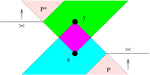
Figure 11: The arrows indicate that the lower side of the right cut is identified with the upper side of the left cut. These identifications include a right-left reflection, so that $(P,P^{*})\in R_{pf}$. The crosses indicate that neither the upper side of the right cut nor the lower side of the left cut is identified with anything. Since $P^{*}\subset I^{+}(x)$ and $P\subset I^{-}(y)$, $(P,P^{*})\in L_{alt}(x,y)$. An infinite set of such cuts and identifications can lead to poor separation properties.

However, in general interior points and ideal points need not be $T_{2}$ separated. The example in figure 11 illustrates the general idea. In this example $(P,P^{*})$ lies in $L_{alt}(x,y)$. This by itself causes no great harm – one may simply work with $z_{1},z_{2}\in I^{+}(x)\cap I^{-}(y)$ so that $L_{alt}(z_{1},z_{2})$ is just the set $\{p\in M:z_{1}\ll p\ll z_{2}\}$. But in similar examples with an infinite number of cuts and identifications, there may be a point $z$ such that some pair resembling $(P,P^{*})$ in figure 11 lies in $L_{alt}(x,y)$, $L_{alt}^{+}(x)$, and $L_{alt}^{-}(y)$ for all $x\ll z,y\gg z$.

In this case it would follow that $z$ is not $T_{2}$ separated from $(P,P^{*})$. The argument is as follows: We have seen that any open set containing $z$ contains some open $U\subset M$ with $U\ni z$. An open set that does not intersect $U$ must be constructed from $\bar{M}\setminus L_{alt}(x,y)$, $\bar{M}\setminus L_{alt}^{+}(x)$, and $\bar{M}\setminus L_{alt}^{-}(y)$. But none of these open sets contain $(P,P^{*})$. Thus, $z$ and $(P,P^{*})$ are not $T_{2}$ separated. With some careful arrangement, one can find similar examples in which a point on a timelike curve $\gamma$ is not $T_{2}$ separated from an endpoint of this curve.

Clearly, this topology has undesirable separation properties. In particular, its failure to recognize the distinction between different IP-IF pairs which have the same future or past is distressing. Furthermore, this is not the only problem: we have argued that in sufficiently complicated examples, interior and boundary points will fail to be $T_{2}$ separated in this topology (and of course none of the problems with separation properties in $\bar{\cal T}$ encountered in section 4.2 are corrected in this topology). Finally, it leads in figure 6 to the convergence of $\{x_{n}\}$ to both $\bar{P}$ and $\bar{Q}$.

Our main purpose in discussing this topology was to show that the non-intuitive behaviour of certain limits in the topology $\bar{\cal T}$ was not purely a consequence of working with the causal structure; certain arbitrary choices in the definition of the topology also affect these limits. The fact that $\bar{\cal T}_{alt}$ generally produces more limit points than $\bar{\cal T}$ is a positive feature in some examples (such as figure 5), but a negative feature in others (such as figure 6). One might hope that there is some more inspired choice of definition, somehow intermediate between the ones we have made, which would allow us to combine the good features of both topologies.

References

- [1] R. Penrose, “Conformal treatment of infinity,” in Relativity, Groups and Topology, ed. C. M. de Witt and B. de Witt, (1964, Gordon & Breach, New York); ibid, “Zero rest-mass fields including gravitation: asymptotic behaviour,” Proc. Roy. Soc. Lond. A 284 (1965) 159.
- [2] R. Geroch, E. H. Kronheimer, and R. Penrose, “Ideal points in space-time,” Proc. Roy. Soc. Lond. A 327 (1972) 545.
- [3] Kuang zhi-quan, Li jian-zeng and Liang can-bin, “-boundary of Taub’s plane-symmetric static vacuum spacetime,” Phys. Rev. D 33 (1986) 1533.
- [4] Kuang zhi-quan and Liang can-bin, “On the GKP and BS constructions of the -boundary,” J. Math. Phys. 29 (1988) 433.
- [5] I. Rácz, “Causal boundary of space-times,” Phys. Rev. D 36 (1987) 1673; ibid, “Causal boundary for stably causal space-times,” Gen. Rel. Grav. 20 (1988) 893.
- [6] Kuang zhi-quan and Liang can-bin, “On the Rácz and Szabados constructions of the -boundary,” Phys. Rev. D 46 (1992) 4253
- [7] R. Budic and R. K. Sachs, “Causal boundaries for general relativistic space-times,” J. Math. Phys. 15 (1974) 1302.
- [8] L. Szabados, “Causal boundary for strongly causal space-time,” Class. Quant. Grav. 5 (1988) 121;
- [9] L. Szabados, “Causal boundary for strongly causal space-time II,” Class. Quant. Grav. 6 (1989) 77.
- [10] A. Garcia-Parrado and J. M. Senovilla, “Causal relationship: A new tool for the causal characterization of Lorentzian manifolds,” arXiv:gr-qc/0207110.
- [11] D. Marolf and S. F. Ross, “Plane waves: To infinity and beyond!,” arXiv:hep-th/0208197.
- [12] P. Rübe, “An example of a nontrivial causally simple spacetime having interesting consequences for boundary conditions”, J. Math. Phys. 31 (1990) 868.
- [13] E. H. Kronheimer and R. Penrose, “On the structure of causal spaces,” Proc. Camb. Phil. Soc. 63, (1967) 481.
- [14] R. D. Sorkin and E. Woolgar, “A causal order for space-times with C0 Lorentzian metrics: Proof of compactness of the space of causal curves,” Class. Quant. Grav. 13, 1971 (1996) [arXiv:gr-qc/9508018].
- [15] D. Berenstein and H. Nastase, “On lightcone string field theory from super Yang-Mills and holography,” arXiv:hep-th/0205048.
- [16] M. W. Brinkmann, “On Riemann spaces conformal to Euclidean spaces,” Proc. Natl. Acad. Sci. U.S., 9 (1923) 1, see section 21.5.
- [17] H. Bondi, F.A.E. Pirani, and I. Robinson, “Gravitational waves in general relativity III: Exact plane waves,” Proc. Roy. Soc. Lond. A 251 (1959) 519.
- [18] J. Hély, Compt. rend. 249 (1959) 1867.
- [19] A. Peres, “Some Gravitational Waves,” Phys. Rev. Lett. 3, 571 (1959) [arXiv:hep-th/0205040].
- [20] J. Ehlers and W. Kundt, “Exact Solutions of the gravitational field equations” in Gravitation: An introduction to current research, ed. by L. Witten (Wiley, New York, 1962).
- [21] D. Kramer, H. Stephani, E. Herlt, M. MacCallum, and E. Schmutzer, Exact Solutions of Einstein’s field equations (Cambridge, 1979).
- [22] D. Marolf and S. F. Ross, “Plane waves and spacelike infinity” [arXiv:hep-th/0303044].
- [23] V. E. Hubeny and M. Rangamani, “Causal structures of pp-waves,” JHEP 0212 (2002) 043 [arXiv:hep-th/0211195]