Simultaneous bounds on the gravitational dipole radiation and varying gravitational constant from compact binary inspirals

Abstract

Compact binaries are an important class of gravitational-wave (GW) sources that can be detected by current and future GW observatories. They provide a testbed for general relativity (GR) in the highly dynamical strong-field regime. Here, we use GWs from inspiraling binary neutron stars and binary black holes to investigate dipolar gravitational radiation (DGR) and varying gravitational constant predicted by some alternative theories to GR, such as the scalar-tensor gravity. Within the parametrized post-Einsteinian framework, we introduce the parametrization of these two effects simultaneously into compact binaries’ inspiral waveform and perform the Fisher-information-matrix analysis to estimate their simultaneous bounds. In general, the space-based GW detectors can give a tighter limit than ground-based ones. The tightest constraints can reach $\sigma_{B}<3\times 10^{-11}$ for the DGR parameter $B$ and $\sigma_{\dot{G}}/G<7\times 10^{-9}\,{\rm yr}^{-1}$ for the varying $G$, when the time to coalescence of the GW event is close to the lifetime of space-based detectors. In addition, we analyze the correlation between these two effects and highlight the importance of considering both effects in order to arrive at more realistic results.

1 Introduction

Until now, Einstein’s theory of general relativity (GR) [1] is a widely accepted theory passing a bulk of precise experimental tests with flying colors [2]. Nevertheless, there still exist a vast amount of motivations to explore alternative theories of gravity. Theoretically, the incompatibility between GR and quantum mechanics remains to be solved. From the experimental point of view, GR hardly explains the observations like the cosmic inflation and anomalous kinematics of galaxies without introducing the unknown dark energy or dark matter [3]. GR is still an imperfect theory of gravity to a certain extent. As an effort to go beyond GR, various extensions and modifications to GR were proposed [3]. Among possible modifications to GR from numerous perspectives, we consider time variation of the gravitational constant $G$ and the dipolar gravitational radiation (DGR) in this work. These two aspects represent some popular strawman targets for phenomenological studies of gravity [2].

In GR, the gravitational coupling strength $G$ is a constant independent of space and time. However, this cannot be taken for granted. Dirac [4, 5] first came up with the possibility of a time-varying $G$, hinted by his large number hypothesis. Theoretically, some alternative theories of gravity indicate a varying gravitational constant, notably in scalar-tensor theories (STTs) [6, 7], higher-dimensional theories [8, 9, 10], and string theories [11, 12]. There are lots of experiments for testing gravity with the time-varying $G$ effect, such as lunar laser ranging experiments [13, 14, 15], radio observations of binary pulsars [16, 17, 18, 19], cosmic microwave background observations [20], and Big Bang nucleosynthesis [21, 22].

A time-varying $G$ in most alternative theories is often accompanied by the existence of one or more extra degrees of freedom in the gravitational sector. For instance, the Jordan-Fierz-Brans-Dicke (JFBD) theory [6, 23, 24, 25]—one of the simplest natural alternative STTs—involves an additional scalar field $\phi$, which indicates a varying $G$ via $G\propto{\phi}^{-1}$ when $\phi$ is time dependent [26]. In addition, additional gravitational degrees of freedom can usually cause extra DGR in these alternative theories of gravity [26, 27, 28, 29], while neither monopole nor dipole radiation exists in GR. DGR is characterized by a parameter $B$ which vanishes in GR [28]. As an extra channel of energy dissipation, DGR enhances the orbital decay in a binary system. Therefore, in some alternative theories it is advised to investigate these two non-GR corrections simultaneously [30, 31, 32].

In the weak-field regime, bounds have been put which can be associated to DGR [33]. However, the weak-field experiments are not always applicable to the strong-field regime [34]. In this case, one needs to investigate the motion of strongly self-gravitating bodies, such as neutron stars (NSs) and black holes (BHs), which can more easily deviate from the GR expectation in some modified gravity theories [28].

To explore DGR, binary pulsars in the quasi-stationary strong-field regime turn out to be ideal testbeds [18, 32, 35, 36, 37, 38]. The emitted radio pulses from binary pulsars can be continuously monitored by large radio telescopes. With the technology called pulsar timing, the parameters of binary pulsars can be measured to high precision and be used to detect or constrain the varying-$G$ and DGR effects simultaneously, as was done in Refs. [30, 31, 39]. One of the best results came from a combination of PSRs J0437$-$4715, J1713$+$0747, and J1738$+$0333 [31], which simultaneously constrained $\sigma_{\dot{G}}/G<10^{-12}\,{\rm yr}^{-1}$ and $\sigma_{B}<10^{-7}$ at the 68% confidence level (CL).

Pulsars can put tight limits on varying-$G$ and DGR effects in several gravitational theories, including the JFBD theory. In JFBD theory, binary NS (BNS) inspirals can emit DGR while binary BHs (BBHs) cannot, because of the no-hair theorem for BHs [40, 41]. However, there also exist other STTs which predict DGR predominantly (or only) in BBHs, e.g. the shift-symmetric Horndeski theories [42]. In those STTs where DGR only comes from systems involving BHs, pulsar observations cannot put limits, and we have to resort to other means, e.g., via gravitational-wave (GW) observations.

Up to now, about a hundred GWs have been announced by the LIGO/Virgo/KAGRA Collaboration from their observing runs O1, O2 and O3 [43, 44, 45], including the first BBH event GW150914 [46] and the first BNS event GW170817 [47]. A large number of events are expected in the near future [48]. GW signals are detected by GW interferometers, and analysis based on the matched-filtering method recovers the information about the dynamics of its source [49]. They can also be used to put constraints on the non-GR effects [50, 51, 52, 53, 54, 55]. Currently, all observed GWs come from compact binary coalescences in the highly dynamical strong-field regime, providing another powerful testbed besides binary pulsars. Some earlier studies [51, 56, 57] have already used binary pulsars and GWs to constrain the DGR and the varying-$G$ effects. However, these works usually focus on one aspect, and do not include varying $G$ and DGR simultaneously.

The corresponding phase corrections due to the varying-$G$ and DGR effects are at the $-4$ post-Newtonian (PN) and $-1$ PN orders respectively. In general, relative to binary pulsars, BNS inspirals have a larger binary velocity $v$, leading to weaker constraints. The bounds from BBH systems are usually several orders of magnitude looser than those from BNSs for the ground-based GW detectors, while for space-based GW detectors there is no such big difference. This is because that BBH inspirals stay in the ground-based detectors’ frequency bands for a shorter time relative to BNS inspirals. Similarly, in general, space-based detectors can give tighter limits than ground-based detectors for negative PN effects, because of their higher sensitivities in the low-frequency band [50].

In this work, we use the Fisher information matrix (FIM) [49] to investigate the prospects of testing the varying-$G$ and DGR effects simultaneously with GW observations of BNSs and BBHs. We consider both ground-based and space-based GW detectors, including the Advanced Laser Interferometer Gravitational-Wave Observatory (AdvLIGO) [48], the third-generation GW detectors like the Einstein Telescope (ET) [58, 59, 60] and Cosmic Explorer (CE) [61, 62, 63], the proposed space-based decihertz GW detectors like the Decihertz Observatory (DO) [64, 65] and the DECi-hertz Interferometer Gravitational wave Observatory (DECIGO) [66, 67] (see Table 1). For compact binaries, we use GW150914 and GW170817 as examples of BBH and BNS events respectively.

From our study, for BNSs B-DECIGO can give the tightest constraints on DGR for GW170817-like events, being four orders of magnitude tighter than binary pulsars [31]. However, the constraints from AdvLIGO are looser than those from binary pulsars. As for $\dot{G}$, the tightest bound from GW170817-like events is still about four orders of magnitude looser than binary pulsars [31]. These are in accordance with the above discussions. We emphasize that, for some alternative gravity theories, only simultaneous bounds on the varying-$G$ and DGR effects using GW events are creditable because of the strong correlation between them. The absolute correlation coefficient between them can reach $\sim 0.8$ or higher, and individual bounds on these effects are only $15\%$–$40\%$ of the simultaneous bounds. The constraints on DGR without considering the varying-$G$ effect are thus over-optimistic for some specific alternative theories and vice versa.

We organize the paper as follows. We summarize the main calculation method, namely the FIM, in Sec. 2. In Sec. 3 we introduce briefly the modified waveform template of GW inspiral signals of compact binaries and the GW detectors we use. In Sec. 4 we use the FIM to obtain joint constraints on the varying-$G$ and DGR phenomena from simulated BNS and BBH GW events. Conclusions are summarized in Sec. 5. Throughout the paper, we use the geometrized unit where $G=c=1$.

2 Fisher information matrix

The matched-filtering analysis is the prescription used for parameter estimation of GWs. We briefly review its general procedure here. Firstly, the noise-weighted inner product of two signals $h(t)$ and $g(t)$ is defined by [49]

$$(h\,,g)=4\Re\int_{f_{\rm min}}^{f_{\rm max}}\frac{\tilde{h}(f)^{*}\tilde{g}(f)}{S_{n}(f)}{\rm d}f\,,$$ (1)

where $\tilde{h}(f)$ and $\tilde{g}(f)$ are Fourier transformations of signals $h(t)$ and $g(t)$ respectively. In Eq. 1, $S_{n}(f)$ is the one-sided power spectral density (PSD) of the noise. The signal-to-noise ratio (SNR) of a signal $h$ in the detector is defined as $\rho=(h,h)^{1/2}$. Characterizing the strength of the signal, SNR is an important criterion to assess whether we have detected a real GW event from the strain data. In general, we set the critical SNR to $\rho=8$ for ground-based GW detectors, and $\rho=15$ for space-based detectors [69, 70].

FIM is a useful tool for estimating the measurement uncertainties of GW events [49, 71]. It is defined as,

$$F_{ij}=\left(\frac{\partial h}{\partial\theta_{i}}\,,\frac{\partial h}{\partial\theta_{j}}\right)\,,$$ (2)

where $\theta_{i}$ and $\theta_{j}$ are the $i$-th and $j$-th parameters of the GW waveform template $h$. Assuming a uniform prior, the inverse of the FIM yields the covariance between the parameters in the posterior distribution, which is approximately Gaussian in the high SNR limit or equivalently in the linear signal approximation (LSA) [71, 72]. This approximation of the full posterior can be proved by expanding the detected signal around the true parameters up to the first order and substituting the expansion into the Bayesian posterior [71]. Defining the inverse of FIM as $\Sigma\equiv F^{-1}$, one can obtain the standard deviations and correlation coefficients of the parameters

$$\sigma_{i} =\sqrt{\Sigma_{ii}}\,,$$ (3)

$$c_{ij} =\frac{\Sigma_{ij}}{\sigma_{i}\sigma_{j}}=\frac{\Sigma_{ij}}{\sqrt{\Sigma_{ii}\Sigma_{jj}}}\,,$$ (4)

where $\sigma_{i}$ is the standard deviation of the $i$-th parameter, and $c_{ij}$ is the correlation coefficient between the $i$-th and $j$-th parameters [49, 71].

3 Compact binary signals and GW observatories

Compact binary coalescences are highly dynamical gravitational systems whose evolutions are described by inspiral, merger, and ringdown stages. The GW waveform we use is from the inspiral stage assuming a quasi-circular orbit with a quasi-adiabatic inspiral due to the emission of GWs [26, 73, 74]. Generally, the GW waveform in the Fourier domain $\tilde{h}(f)$ is written as a function of the GW frequency $f$ in the following restricted form

$$\tilde{h}(f)=\mathcal{A}f^{-7/6}e^{\mathrm{i}\Psi(f)}\,,$$ (5)

where $\mathcal{A}$ and $\Psi(f)$ stand for the amplitude and the phase, respectively.

In GR, the GW amplitude of a compact binary inspiral signal at the leading order (i.e. the Newtonian order) is

$$\mathcal{A}_{\rm{GR}}=\frac{2}{5}\times\sqrt{\frac{5}{24}}\pi^{-2/3}\frac{\mathcal{M}^{5/6}}{d_{L}}\,,$$ (6)

with $d_{L}$ the luminosity distance, $\mathcal{M}\equiv\eta^{3/5}M_{z}$ the redshifted chirp mass, where $M_{z}\equiv(1+z)M$ with $M$ the sum of the source-frame component masses $m_{1}$ and $m_{2}$, and $\eta=m_{1}m_{2}/M^{2}$ is the symmetric mass ratio. This amplitude has been averaged over the sky position and polarization of GWs as well as the orientation of the binary [54, 67], leading to the factor “$2/5$” in the place of a function dependent on those angles.

Cutting at $3.5$ PN, the inspiral phase of the binary in GR reads [74, 75]

$$\Psi_{\rm{GR}}(f)= 2\pi ft_{c}-\Phi_{c}-\frac{\pi}{4}+\frac{3}{128\eta}\mathfrak{u}^{-5/3}\left\{1+\left(\frac{3715}{756}+\frac{55}{9}\eta\right)\mathfrak{u}^{2/3}-16\pi\mathfrak{u}\right.$$

$$+\left(\frac{15293365}{508032}+\frac{27145}{504}\eta+\frac{3085}{72}\eta^{2}\right)\mathfrak{u}^{4/3}+\pi\left(\frac{38645}{756}-\frac{65}{9}\eta\right)(1+\ln\mathfrak{u})\mathfrak{u}^{5/3}$$

$$+\left[\frac{11583231236531}{4694215680}-\frac{640}{3}\pi^{2}-\frac{6848}{21}\gamma_{\rm E}-\frac{6848}{63}\ln(64\mathfrak{u})+\left(-\frac{15737765635}{3048192}+\frac{2255}{12}\pi^{2}\right)\eta\right.$$

$$\left.\left.+\frac{76055}{1728}\eta^{2}-\frac{127825}{1296}\eta^{3}\right]\mathfrak{u}^{2}+\pi\left(\frac{77096675}{254016}+\frac{378515}{1512}\eta-\frac{74045}{756}\eta^{2}\right)\mathfrak{u}^{7/3}\right\}\,,$$ (7)

where $\mathfrak{u}\equiv\pi M_{z}f$, $t_{c}$ and $\Phi_{c}$ are time and phase at coalescence, $\gamma_{\rm E}$ is the Euler constant. Here, we neglect the spin effects in the GW waveform. Equation 5 with Eqs. 6 and 3 gives the so-called “restricted TaylorF2 waveform” [74] characterizing the inspiral signal in GR. It is valid until the end of the inspiral when the binary comes to the innermost stable circular orbit (ISCO) and plunges into a merger. Thus, the $f_{\max}$ in the inner product of Eq. 1 is chosen to be $f_{\max}=\min\left\{f_{\rm upper},f_{\rm ISCO}\right\}$, where $f_{\rm upper}$ and $f_{\rm ISCO}$ are the upper limit of the detector’s frequency range and the GW frequency corresponding to the ISCO respectively. In different alternative theories of gravity, the evolution of BNSs is modified, leaving non-GR imprints in the amplitude and the phase of GWs.

The varying $G$ makes a difference to the orbital dynamics in various aspects. First of all, time variations of $G$ cause corrections in orbital frequency since $f_{\rm orb}\simeq\sqrt{GM/{4\pi^{2}\,r^{3}}}$ in the Newtonian approximation, where $r$ is the orbital separation. Secondly, the decay of the orbital frequency is also modified, as the amount of energy being lost from binary systems due to emission of GWs is different [27]. In addition, there can be time variations of component masses along with their sensitivities defined by $s=-\partial\ln m/{\partial\ln G}$ [26], as well as non-conservation of the binding energy due to an acceleration caused by time variations in $G$ or masses [50].

To include the varying-$G$ effect in the waveform, the following GW phase modification corresponding to a $-4$ PN term is added to the phase [50],

$$\Psi_{\rm{-4\,PN}}(f)=-\frac{25}{851968}\frac{\dot{G}\mathcal{M}}{\eta^{13/5}}\left(11-\frac{35}{2}S-\frac{41}{2}\sqrt{1-4\eta}\Delta S\right)\mathfrak{u}^{-13/3}\,,$$ (8)

where $S\equiv s_{1}+s_{2}$ and $\Delta S\equiv s_{1}-s_{2}$ with the component sensitivities $s_{1}$ and $s_{2}$. For a NS, the sensitivity $s$ is dependent on its mass and equation of state, and a reasonable approximation is [31]

$$s_{i}\simeq\frac{0.16}{1.33M_{\odot}}m_{i}\,.$$ (9)

For a BH, we fix its sensitivity to $s=0.5$ [76].

The DGR affects the binary evolution by shedding additional energy and momentum, which leads to a faster orbital decay rate and an earlier coalescence [28]. The strength of DGR is parameterized by $B$ characterizing the extra energy loss due to DGR, which is defined via [28],

$$\dot{E}_{\rm{GW}}=\dot{E}_{\rm{GR}}\left[1+B\left(\frac{M}{r}\right)^{-1}\right]\,.$$ (10)

For example, in JFBD-like theory, $B=5(\Delta\alpha)^{2}/96$, where $\Delta\alpha$ is the difference of the scalar couplings of the two bodies. While the determination of $B$ depends on specific gravity theory, the DGR modification to the waveform is general, which reads,

$$\Psi_{\rm{-1\,PN}}(f)=-\frac{3}{224\eta}B\mathfrak{u}^{-7/3}\,.$$ (11)

As for the amplitude, the modifications from DGR and varying-$G$ effects are subdominants, which can be ignored. The phase plays a more important role in GW analysis than amplitude in the matched-filtering method. Therefore, in this work we choose

$$\mathcal{A}=\mathcal{A}_{\rm{GR}}\,,$$ (12)

$$\Psi(f)=\Psi_{\rm{GR}}(f)+\Psi_{\rm{-1\,PN}}(f)+\Psi_{\rm{-4\,PN}}(f)\,,$$ (13)

as the waveform template for the inspiral signals.

We consider the following two types of GW detectors: (i) ground-based laser interferometers, including AdvLIGO and Voyager, as well as the third-generation ones like ET [58] and CE [61, 62, 63]; and (ii) proposed space-based decihertz GW detectors, DO-Conservative [64] and B-DECIGO [66, 67]. The AdvLIGO, together with the advanced Virgo and KAGRA, has discovered about a hundred GW events up to now [43, 44, 45]. Voyager, ET and CE are proposed detectors for observing GWs extending the AdvLIGO’s frequency range with higher sensitivities, while DO-Conservative and B-DECIGO are proposed to observe GWs in the decihertz frequency band. With the improvement of sensitivity, complimentary detection bands, and an increase in the number of detectors, more GW events from a wider range of source populations are expected to be detected. Note that a lower accessible frequency means a longer observational time, whereas the observation time will be limited by the lifetimes of the detectors. This will lead changes to the $f_{\min}$ parameter in the integral range of the inner product of Eq. 1. We choose the lifetime as 4 years for space-based detectors. Therefore, the $f_{\min}$ in Eq. 1 is taken as $f_{\min}=\max\left\{f_{\rm lower},f_{\rm 4\,yr}\right\}$, where $f_{\rm lower}$ is the low limit of the detector’s frequency range and $f_{\rm 4\,yr}$ is determined by

$$f_{\rm 4\,yr}=\left({f_{\rm max}^{-8/{3}}}+\frac{256\pi^{8/3}}{5}{\cal M}^{5/3}\cdot\Delta t_{\rm obs}\right)^{-3/8}\,,$$ (14)

where $\Delta t_{\rm obs}={\rm 4\,yr}$, and $f_{\rm max}$ is defined above. As for the ground-based detectors, we choose $f_{\min}=f_{\rm lower}$.

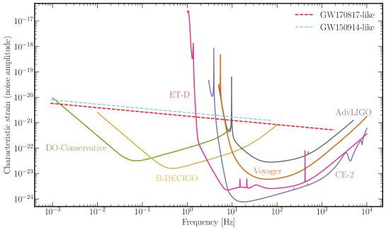
Figure 1: The dimensionless pattern-averaged characteristic inspiral strains of GW150914-like and GW170817-like events, in contrast to the dimensionless noise spectral density of the detectors. The characteristic strains are averaged over sky location and polarization angle of the source, ignoring the spin contribution and truncating at $f_{\rm{ISCO}}$. The noise is plotted according to the configurations listed in Table 1.

Table 1: Characteristics of GW detectors.

Detector	$n$	$F$	Configuration	$f_{\rm lower}\,[{\rm Hz}]$	$f_{\rm upper}\,[{\rm Hz}]$	Schedule	Reference
DO-Conservative	2	$\sqrt{3}/2$	Triangle	0.001	10	2035-2050	Ref. [64, 65]
B-DECIGO	2	$\sqrt{3}/2$	Triangle	0.01	100	2020s	Ref. [68]
AdvLIGO	2	1	Rightangle	5	5000	O4	LIGO documentsa
Voyager	2	1	Rightangle	5	10000	Late 2020s	LIGO documentsb
CE-2	2	1	Rightangle	3	10000	2040s	Ref. [62, 63]
ET-D	3	$\sqrt{3}/2$	Triangle	1	10000	Mid 2030s	Ref. [58, 60]

• https://dcc.ligo.org/LIGO-T1800044/public

• https://dcc.ligo.org/LIGO-T1500293/public

Table 2: Number of observable BNSs and BBHs per year for different GW detectors. The local BNS and BBH merger rates are chosen as $250\,{\rm Gpc}^{-3}{\rm yr}^{-1}$ and $22\,{\rm Gpc}^{-3}{\rm yr}^{-1}$ respectively  [77]. We adopt two models of merger rate’s time evolution, BNS/A [78, 79] and BNS/B [80], for BNSs, and one model for BBHs [81].

	DO-Conservative	B-DECIGO	AdvLIGO	Voyager	CE-2	ET-D
BNS/A	12	384	50	5424	291264	161273
BNS/B	13	421	52	6831	995039	394203
BBH	70412	85792	866	34997	87021	87244

In Fig. 1, we illustrate the dimensionless pattern-averaged characteristic strain $\tilde{h}_{c}(f)$ of GW150914-like and GW170817-like signals, in contrast to the dimensionless noise spectral density $\tilde{h}_{n}(f)$ of the above detectors [82]. The “GW150914-like” (“GW170817-like”) signal indicates mock GW event that adopts the component masses and distance of real GW150914 (GW170817), but omits the spin effects and uses the angle-averaged waveform in Eqs. 6 and 3. The quantities $\tilde{h}_{c}(f)$ and $\tilde{h}_{n}(f)$ are defined by $2f\big{|}\tilde{h}(f)\big{|}$ and $\sqrt{fS_{n}^{\rm eff}(f)}$ respectively, where $S_{n}^{\rm eff}$ is the effective noise PSD, $S_{n}^{\rm eff}(f)={S_{n}(f)}/{nF^{2}}$, where $n$ and $F$ are the equivalent numbers and the form factor of the detectors. Configurations of detectors are collected in Table 1. In the figure SNRs are proportional to the area between the signals and the noise curves [82].

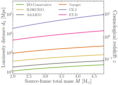
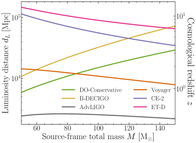
Figure 2: Cosmological reach to equal-mass BNSs (left) and BBHs (right) for different detectors. The $\Lambda$CDM parameters used for calculation are matter density $\Omega_{\rm m}\approx 0.315$, dark energy density $\Omega_{\Lambda}\approx 0.685$, and the Hubble constant $H_{0}\approx 67.4\ \text{km}\,\text{s}^{-1}\,\text{Mpc}^{-1}$ [83]. The thresholds of detection are set to $\rho=8$ and $\rho=15$ for ground-based and space-based detectors, respectively.

The cosmological reach is defined as the corresponding luminosity distance to the detection threshold. In Fig. 2, we plot cosmological reach to equal-mass BNSs and BBHs for different detectors. With the cosmological reaches, we estimate the corresponding BNS and BBH event rates in Table 2, showing the prospect that a large population of BNSs and BBHs can be detected by the above detectors.

4 Simultaneous bounds on $B$ and $\dot{G}$

We will use FIM to obtain simultaneous constraints on DGR and varying-$G$ effects. Let indices $i$ and $j$ in the FIM run through the set of parameters $\{\ln\mathcal{A},\ln\eta,\ln\mathcal{M},t_{c},\Phi_{c},B,\dot{G}\}$. We calculate partial derivatives analytically from the GW waveform (5), and they are shown in A. Substituting values of source parameters together with fiducial values $B=0$ and $\dot{G}=0$, we calculate the FIM through Eq. 2. Then, the standard deviations of $B$ and $\dot{G}$ are obtained from corresponding elements of the inverse of FIM, providing 1-$\sigma$ bounds on DGR and varying-$G$ effects. To convert between luminosity distance and redshift, we adopt the $\Lambda$CDM model with Hubble constant $H_{0}\approx 67.4\ \text{km}\,\text{s}^{-1}\,\text{Mpc}^{-1}$, matter density fraction $\Omega_{\rm m}\approx 0.315$, and vacuum energy density fraction $\Omega_{\Lambda}\approx 0.685$ [83].

Considering how the waveform depends on different parameters before calculation can bring some simplification. The luminosity distance $d_{L}$ does not appear in the phase but in the amplitude as shown in Eq. 6. According to Eqs. (2) and (3), we approximately have $F_{ij}\propto 1/d^{2}_{L}$ and $\sigma_{B}$ (or $\sigma_{\dot{G}}$) $\propto d_{L}$. For BNS events, we use $d_{L}=40\,{\rm Mpc}$, while for BBH events we use $d_{L}=440\,{\rm Mpc}$. In addition, according to Sec. 3, different values of $t_{c}$ and $\Phi_{c}$ do not affect the constraints, and we use fiducial values $t_{c}=0$ and $\Phi_{c}=0$.

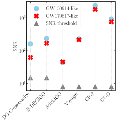
Figure 3: SNRs of GW150914-like and GW170817-like events in different detectors. The gray solid triangles stand for the thresholds of detection with $\rho=8$ and $\rho=15$ for ground-based and space-based detectors respectively.

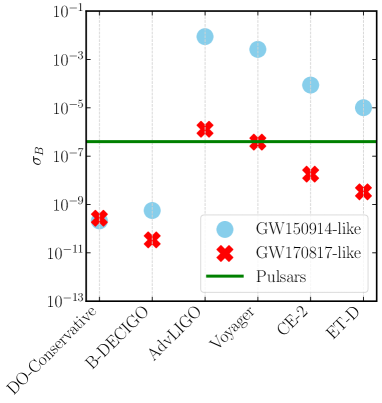
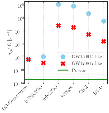
Figure 4: A comparison of $\sigma_{B}$ and $\sigma_{\dot{G}}/G$ in detections of GW150914-like and GW170817-like events using different detectors. Current timing results of pulsars are shown with green lines for comparison.

4.1 Constraints on $B$ and $\dot{G}$

First, we investigate the constraints on $B$ and $\dot{G}$ from different detectors. Figure 3 plots SNRs of GW150914-like and GW170817-like events in different detectors [69]. The SNRs in all detectors are so high that we can use the FIM to estimate the measurement precision of parameters to a good extent [71].

Figure 4 shows the constraints on $B$ and $\dot{G}$ with our two example events in different detectors. They are compared with the bounds from binary pulsars [31]. The space-based GW detectors DO-Conservative and B-DECIGO outperform the other GW detectors even though they do not have the highest SNRs. This can be explained by the lower accessible frequency of these detectors and contributes more to the negative $-1$ PN and $-4$ PN terms in $\Psi(f)$. For the GW170817-like event, the current GW detector AdvLIGO cannot constrain $B$ as tightly as pulsars, while future detectors like DO-Conservative, B-DECIGO, CE, and ET will provide bounds 2 to 4 orders of magnitude tighter. As for $\dot{G}$, the bounds by GW detectors from the GW170817-like event are looser than $\sigma_{\dot{G}}/G<10^{-12}\,{\rm yr}^{-1}$ (68% CL) from pulsars [31]. It is caused by the even more negative PN order of the varying-$G$ effect in the phase correction. Constraints from the GW150914-like event are close to those from the GW170817-like event for space-based GW detectors, but much looser for ground-based ones. Comparing to space-based detectors, there are greater differences of the GW cycles in the frequency bands between BBH and BNS inspirals for ground-based detectors. As mentioned in Sec. 1, though limits from BBHs are not as tight as those from BNSs, they are still meaningful, because observations of pulsars cannot give any limits for BBHs at all [28].

When calculating the SNRs in Fig. 3 and the constraints in Fig. 4, we have chosen $f_{\max}=\min\left\{f_{\rm upper},f_{\rm ISCO}\right\}$ and $f_{\min}=\max\left\{f_{\rm lower},f_{\rm 4\,yr}\right\}$ for space-based detectors, which correspond to the best constraints potentially achievable by those future detectors for the two GW events. In fact, an observed binary will have an initial frequency according to the underlying population, and any other initial frequency different from $f_{\rm min}$ will lead to a lower SNR and looser constraints [84]. In Fig. 5, we plot how the SNR and constraints depend on the initial frequencies of GW150914-like and GW170817-like events for space-like detectors DO-Conservative and B-DECIGO. When the initial frequency $f_{\rm ini}$ is larger than $f_{\rm min}$, the integral range will be $[f_{\rm ini}\,,f_{\max}]\subsetneqq[f_{\rm 4\,yr}\,,f_{\max}]$, corresponding to a lower SNR and looser limits. For those $f_{\rm ini}$ smaller than $f_{\rm min}$, though the DGR and varying-$G$ effects are more significant for lower frequencies, it also takes more time for each circle of the binary in orbital evolution. Limited by the assumed 4-year lifetime of the space-based detectors, for $f_{\rm ini}<f_{\rm 4\,yr}$ we still have lower SNRs and looser constraints, as shown in Fig. 5. Moreover, for those frequencies far away from $f_{\rm 4\,yr}$, the SNRs become even smaller than the detection threshold, not to mention the FM approximation and constraints.

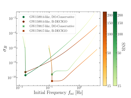
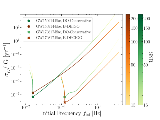
Figure 5: Dependence of $\sigma_{B}$ (left) and $\sigma_{\dot{G}}$ (right) on the initial frequency in DO-Conservative and B-DECIGO detectors, for GW150914-like and GW170817-like events. The color of lines represents the value of the SNR. The $f_{\rm 4\,yr}$ of GW150914-like and GW170817-like events, as well as the corresponding constraints, are marked with “$\bullet$” and “$\times$”.

Then we investigate how a binary’s parameters influence $\sigma_{B}$ and $\sigma_{\dot{G}}$. We choose ET-D and B-DECIGO as the representatives of ground-based and space-based detectors, respectively. We expect the properties of parameter dependence to be alike within the same kind of detector due to their similar sensitivity ranges and shapes.

The constraints on $B$ are shown in Fig. 6. Here, we vary the component masses $m_{1}$ and $m_{2}$. Systems with smaller masses give slightly tighter bounds on $B$. A lighter system has a larger separation when it enters the detector’s sensitivity band, resulting in slower damping and more cycles within the detector bandwidth, and a tighter limit in the end. In Fig. 6, the limits on $B$ only weakly rely on the components of BNSs, varying within one order of magnitude, and all limits are tighter than the pulsar results [31]. For BBHs, there exists strong dependence between $\sigma_{B}$ and BBHs’ component masses. Note that in Eq. 11 the $-1$ PN phase term does not explicitly depend on mass parameters, and the dependence of mass actually originates from the range of integral. A GW signal from a massive BBH will stay in the detector for fewer cycles, leading to looser constraints. This dependence is particularly evident in ET-D which has a relatively high frequency band.

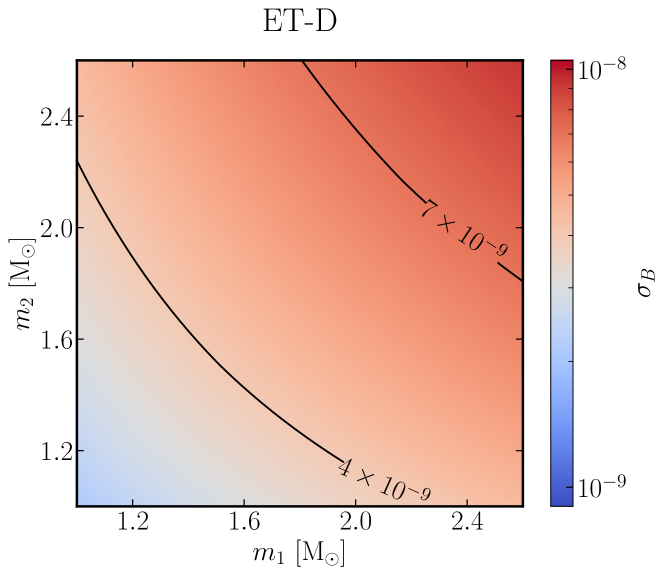
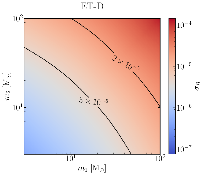
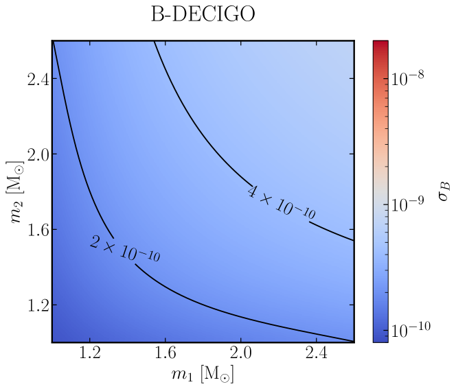
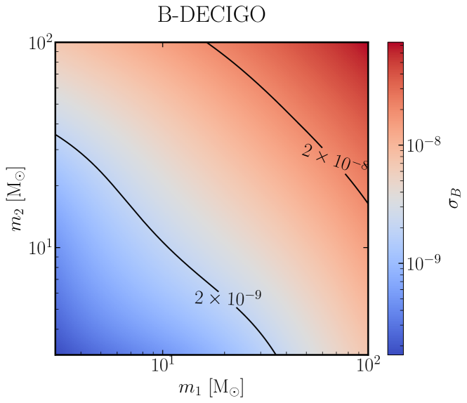
Figure 6: Dependence of $\sigma_{B}$ on component masses in two GW detectors, ET-D (upper) and B-DECIGO (lower), for BNSs (left) and BBHs (right).

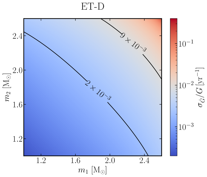
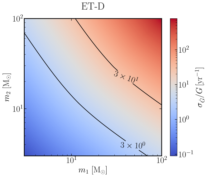
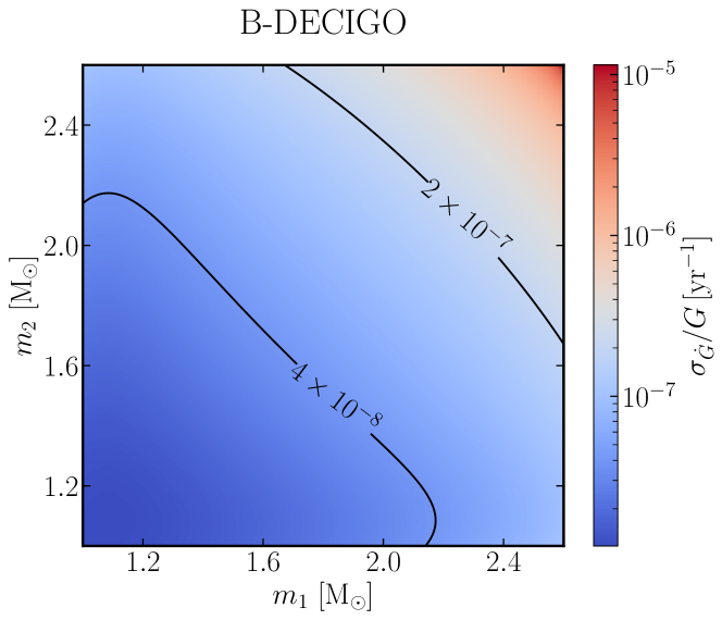
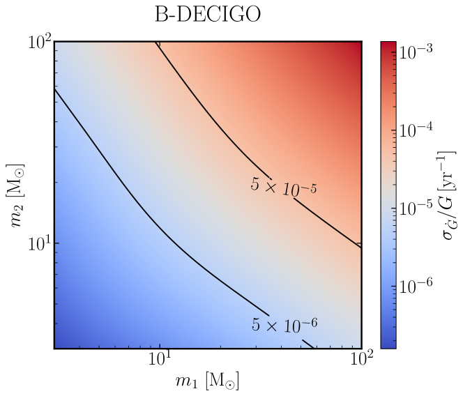
Figure 7: Same as Fig. 6, for $\sigma_{\dot{G}}$.

The phase correction term of varying-$G$ in Eq. 8 is relatively complicated, dependent on four parameters, $m_{1}$, $m_{2}$, $s_{1}$, and $s_{2}$. In Fig. 7, we vary parameters $m_{1}$ and $m_{2}$ in BNS and BBH systems like Fig. 6, and adopt the approximation in Eq. 9 for NSs and fix the sensitivity as $s=0.5$ for BHs. To study the parameter space outside Eq. 9, as discovered in some alternative gravity theories, in Fig. 8 we release the approximation in Eq. 9 and vary all the four parameters for BNS systems. Same as constraining $B$, binaries with larger masses generally give a larger $\sigma_{\dot{G}}$. From our results, all limits on $\sigma_{\dot{G}}$ are looser than results from pulsars [31], because the GW detectors here can hardly reach the low frequency where ${\dot{G}}$’s $-4$ PN effects are as significant as in binary pulsars.

In Fig. 8, $\sigma_{\dot{G}}$ turns out to be very large in some striped-like regions. This is due to singular FIMs. In these regions, $\partial\tilde{h}/{\partial{\dot{G}}}$ almost vanishes. Therefore, FIM is nearly singular, and the corresponding element in the covariance matrix becomes extremely large. To show this, we define a factor “$\mathfrak{F}$” as

$$\mathfrak{F}\equiv\frac{\mathcal{M}}{\eta^{13/5}}\left(11-\frac{35}{2}S-\frac{41}{2}\sqrt{1-4\eta}\Delta S\right)\propto\frac{\partial\tilde{h}(f)}{\partial{\dot{G}}}\,,$$ (15)

and plot lines where $\mathfrak{F}=0$ in Fig. 8. As expected, the regions with large $\sigma_{\dot{G}}$ and the lines where $\mathfrak{F}=0$ are highly consistent. $\mathfrak{F}$ only depends on properties of a binary, so regions with large $\sigma_{\dot{G}}$ in different detectors have the same shape, with differences only in amplitude. Singular (or quasi-singular) FIMs cannot provide credible forecasts of parameter estimation, and alternative analysis methods are required [71, 72]. Though the constraint on $\dot{G}$ becomes extremely loose in the adjacency of the singularities, in most area of the parameter space, $\sigma_{\dot{G}}$ remains to be small. Therefore, BNSs are still in general good sources for constraining $\sigma_{\dot{G}}$, as long as $\mathfrak{F}$ is not close to zero. For BBHs, their sensitivities are fixed as 0.5, so their $\mathfrak{F}$ never equals to zero. Same as the constraints on $B$, BBH inspirals in our study cannot give limits as tight as BNSs and pulsars.

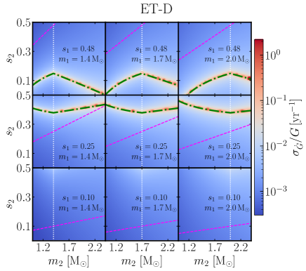
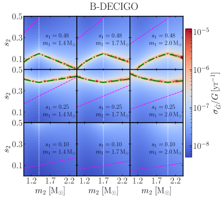
Figure 8: Dependence of $\sigma_{\dot{G}}$ on component masses and sensitivities of BNSs. The green dot-dashed lines correspond to $\mathfrak{F}=0$ [see Eq. (15)], where FIM becomes singular. The fuchsia dashed lines are plotted with the assumption of $s_{2}=m_{2}\cdot s_{1}/m_{1}.$ The white dotted lines show the primary masses of binaries.

4.2 The role of correlation

Though $B$ and $\dot{G}$ show up at different PN orders in the modified GW phase, they are correlated in the posterior distributions. In FIM analysis, the correlation between them is characterized by $c_{B\dot{G}}$ using Eq. 3. The sign of $c_{B\dot{G}}$ changes when crossing the singular region mentioned above, rooting in the sign changing of $\mathfrak{F}$. When calculating the correlation coefficients, we adopt Eq. 9 for BNSs, and fix $s=0.5$ for BBHs. For BBHs (whose masses range from $3\,{M}_{\odot}$ to $100\,{M}_{\odot}$), $\big{|}c_{B\dot{G}}\big{|}$ is almost always greater than 0.9, while for BNSs, $\big{|}c_{B\dot{G}}\big{|}$ is more dependent on the specifics of detectors and system masses. Only in a small region of the parameter space, $\big{|}c_{B\dot{G}}\big{|}$ is smaller than 0.5. Generally, the correlation between $B$ and $\dot{G}$ is smaller for BNS inspirals than BBH inspirals, and space-based detectors give a smaller correlation than ground-based detectors. For BNSs, the space-based detectors can distinguish $-1$ PN and $-4$ PN effects better with a lower frequency band, giving a relatively small correlation. But in a BBH inspiral, $\dot{G}$’s $-4$ PN effects hardly enter the frequency bands of both ground-based and space-based detectors, leading to a strong correlation between $B$ and $\dot{G}$. In all, for almost any signal from BNSs or BBHs, we expect $B$ and $\dot{G}$ to be strongly correlated.

In order to acquire the visualized insight of the correlation between $B$ and $\dot{G}$, we use two types of detectors, ET-D and B-DECIGO, and two typical GW events, GW150914-like and GW170817-like, as examples. In Fig. 9 we plot the $68\%$ confidence levels of the joint posterior distributions of $B$ and $\dot{G}$ using the FIM method. The 2-dimensional Gaussian distribution of $B$ and $\dot{G}$ can be obtained from the FIM,

$$P(B,\dot{G})=\frac{1}{2\pi\sigma_{B}\sigma_{\dot{G}}\sqrt{1-c_{B\dot{G}}^{2}}}\exp\left\{-\frac{1}{2\left(1-c_{B\dot{G}}^{2}\right)}\left[\frac{B^{2}}{\sigma_{B}^{2}}-2c_{B\dot{G}}\frac{B\,\dot{G}}{\sigma_{B}\sigma_{\dot{G}}}+\frac{\dot{G}^{2}}{\sigma_{\dot{G}}^{2}}\right]\right\}\,.$$ (16)

To make a comparison with the situation where $B$ or $\dot{G}$ is overlooked, we re-apply the FIM method to the parameter sets with $\{\ln\mathcal{A},\ln\eta,\ln\mathcal{M},t_{c},\Phi_{c},\dot{G}\}$ and $\{\ln\mathcal{A},\ln\eta,\ln\mathcal{M},t_{c},\Phi_{c},B\}$ to calculate the bound on $\dot{G}$ and $B$ alone, keeping the same values of the other parameters. We represent these individual bounds by grey bands in Fig. 9. As shown in the figure, the widths of the individual bounds are two to three times narrower than the lengths of the corresponding simultaneous bounds, meaning that the individual bounds turn out to be optimistic in the parameter estimations. Calculation proves that the ratio of simultaneous and individual bounds is $(1-c_{B\dot{G}}^{2})^{-1/2}$. So the more that $\big{|}c_{B\dot{G}}\big{|}$ approaches 1, the stronger the correlation between $B$ and $\dot{G}$ is, and the less authentic the individual bounds are. In Fig. 9, $\big{|}c_{B\dot{G}}\big{|}$ is between $0.84$ and $0.94$, and the simultaneous bounds on these two parameters are about $2$ to $3$ times of the individual bounds. Therefore, simultaneous analysis of $B$ and $\dot{G}$ is important for more precise results.

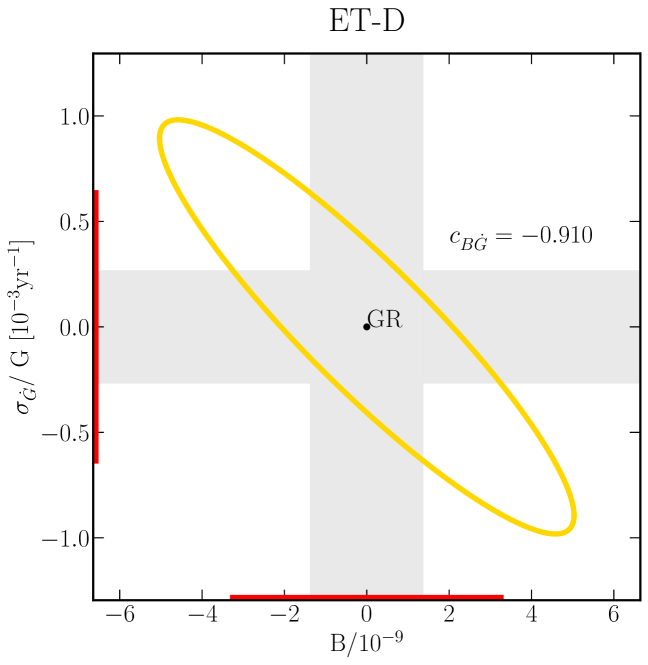
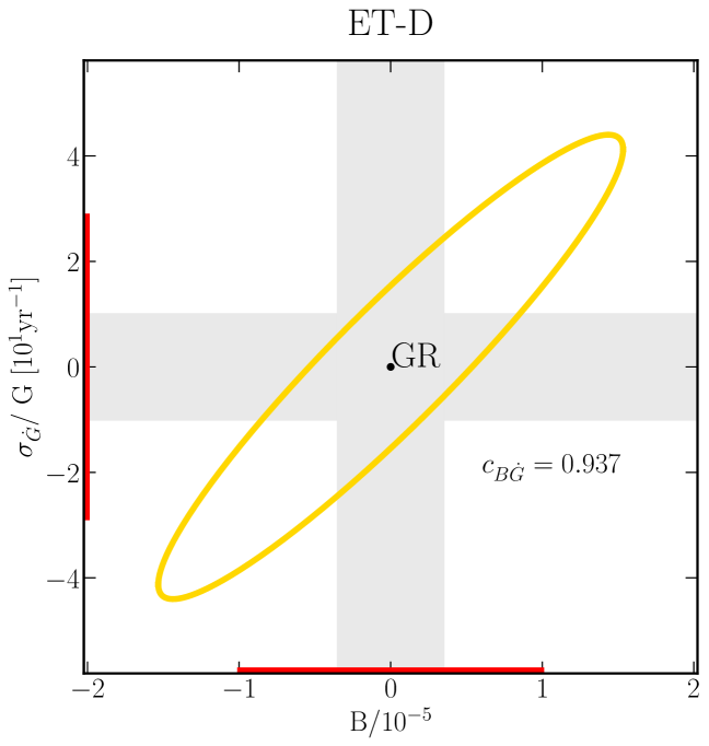
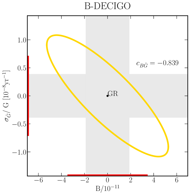
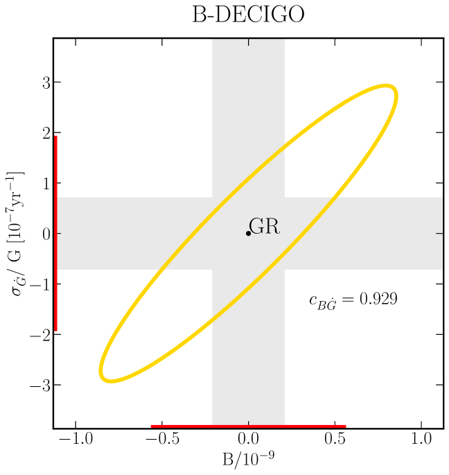
Figure 9: Yellow ellipses are the 1-$\sigma$ contours of the joint distribution of $B$ and $\dot{G}$, marginalizing over other parameters. The standard deviations of $B$ and $\dot{G}$ are indicated by the red error bars. Grey bands stand for the standard deviations of $B$ and $\dot{G}$ when one of them is ignored. The left two panels are for the GW170817-like event, while the right panels are for the GW150914-like event.

5 Discussions

GW has become a promising platform for GR tests. In this work, we consider two important phenomena of violating GR, namely DGR and a varying $G$. These two effects can occur simultaneously in some alternatives to GR. Though occurring at different PN orders in the GW phase, they end up strongly correlated in GW analysis. We show the simultaneous effects of constraining DGR and varying-$G$ effects using compact binary inspirals to be detected by present and future GW detectors. We focus on two kinds of GW detectors, space-based and ground-based laser interferometers. Using FIM, we investigate simultaneous bounds on $B$ and $\dot{G}$ from inspiraling BNSs and BBHs. The main results are summarized as follow.

1. Benefiting from the relatively lower accessible frequencies, space-based detectors make optimal output for constraining varying-$G$ and DGR effects.

2. Generally, BNSs can provide tighter bounds than BBHs on both $B$ and $\dot{G}$. This is particularly evident for ground-spaced detectors. However, limits from BBH inspirals are useful in some alternatives to GR, where DGR predominantly (or only) comes from systems involving BHs [28], while BNSs or pulsars cannot give any constraints.

3. We compare the bounds on $B$ and $\dot{G}$ from BNSs with those from pulsars. Among the detectors we investigated, B-DECIGO can obtain the best constraints with GW170817-like BNSs, reaching $B<3.4\times 10^{-11}$ and $\sigma_{\dot{G}}/G<7.1\times 10^{-9}\,{\rm yr}^{-1}$ (68% CL). The bound on $B$ is about 4 orders of magnitude tighter than pulsar results [31]. For $\dot{G}$, bounds from all detectors are looser than pulsar results, because the effects of $\dot{G}$ are more significant in the lower frequency stage of inspiral. Still, the BNS inspiral signals provide limits in a highly dynamical strong-field regime, which is complementary to pulsars in a quasi-stationary strong-field regime. We look forward to testing varying-$G$ and DGR effects in the highly dynamical strong-field regime with BNS GW observations.

4. We also examine the correlation of $B$ and $\dot{G}$ to find out the necessity of a joint analysis for some alternative gravity theories. The correlation between them is generally strong, as indicated by $\big{|}c_{B\dot{G}}\big{|}\gtrsim 0.8$ in most detectors for GW150914-like and GW170817-like events. This makes the individual bounds two to three times more optimistic than simultaneous bounds. So we suggest to carry out simultaneous estimations on both effects in future GW observations.

Our investigation can be improved by including the population distribution of binary systems to obtain a more realistic study. Considering the binary population can give a weighted average of constraints on $B$ and $\dot{G}$, which would be more practical and meaningful. Also, for space-based detectors we have used the conservative configurations of sensitivities, and better sensitivities might be available when detectors start operating in the future. Finally, in some regions of the parameter space the FIMs become singular, so in this case we require further treatment to obtain credible constraints, for example, by including the merger part of waveform.

Appendix A Equations used in FIM calculation

Partial derivatives of the waveform used in FIM calculation are listed below.

$$\frac{\partial\tilde{h}(f)}{\partial\ln\mathcal{A}} =\tilde{h}(f)\,,$$ (17)

$$\frac{\partial\tilde{h}(f)}{\partial\ln\eta} =\frac{\mathrm{i}}{\eta}\mathfrak{u}^{-5/3}\left\{-\frac{1025}{851968}\frac{\dot{G}\mathcal{M}\Delta S}{\sqrt{1-4\eta}\eta^{3/5}}\mathfrak{u}^{-8/3}-\frac{3}{560}B\mathfrak{u}^{-2/3}+\left(-\frac{743}{16128}+\frac{11}{128}\eta\right)\mathfrak{u}^{2/3}\right.$$

$$+\left.\frac{9}{40}\pi\mathfrak{u}+\left(-\frac{3058673}{5419008}+\frac{5429}{21504}\eta+\frac{617}{512}\eta^{2}\right)\mathfrak{u}^{4/3}+\pi\left(-\frac{7729}{4032}-\frac{38645}{32256}\ln\mathfrak{u}+\frac{13}{128}\eta\right)\mathfrak{u}^{5/3}\right.$$

$$+\left[-\frac{11328104339891}{166905446400}+6\pi^{2}+\frac{321}{35}\gamma_{\rm E}+\frac{107}{35}\ln(64\mathfrak{u})\right.+\left(\frac{3147553127}{130056192}-\frac{451}{512}\pi^{2}\right)\eta$$

$$\left.\left.+\frac{15211}{18432}\eta^{2}-\frac{25565}{6144}\eta^{3}\right]\mathfrak{u}^{2}+\pi\left(-\frac{15419335}{1548288}-\frac{75703}{32256}\eta-\frac{14809}{10752}\eta^{2}\right)\mathfrak{u}^{7/3}\right\}\tilde{h}(f)\,,$$ (18)

$$\frac{\partial\tilde{h}(f)}{\partial\ln\mathcal{M}} =\frac{\mathrm{i}}{\eta}\mathfrak{u}^{-5/3}\left\{-\frac{5}{128}+\frac{{\dot{G}}\mathcal{M}}{\eta^{8/5}}\left(\frac{1375}{1277952}-\frac{4375}{2555904}\mathcal{S}-\frac{5125}{2555904}\sqrt{1-4\eta}\Delta S\right)\mathfrak{u}^{-8/3}+\frac{1}{32}B\mathfrak{u}^{-2/3}\right.$$

$$+\left(-\frac{3715}{32256}-\frac{55}{384}\eta\right)\mathfrak{u}^{2/3}+\frac{\pi}{4}\mathfrak{u}+\left(-\frac{15293365}{65028096}-\frac{27145}{64512}\eta-\frac{3085}{9216}\eta^{2}\right)\mathfrak{u}^{4/3}+\pi\left(\frac{38645}{32256}-\frac{65}{384}\eta\right)\mathfrak{u}^{5/3}$$

$$+\left[\frac{10052469856691}{600859607040}-\frac{5}{3}\pi^{2}-\frac{107}{42}\gamma_{\mathrm{E}}-\frac{107}{126}\ln(64\mathfrak{u})+\left(-\frac{15737765635}{390168576}+\frac{2255}{1536}\pi^{2}\right)\eta\right.$$

$$\left.\left.+\frac{76055}{221184}\eta^{2}-\frac{127825}{165888}\eta^{3}\right]\mathfrak{u}^{2}+\pi\left(\frac{77096675}{16257024}+\frac{378515}{96768}\eta-\frac{74045}{48384}\eta^{2}\right)\mathfrak{u}^{7/3}\right\}\tilde{h}(f)\,,$$ (19)

$$\frac{\partial\tilde{h}(f)}{\partial t_{c}} =\mathrm{i}2\pi f\tilde{h}(f)\,,$$ (20)

$$\frac{\partial\tilde{h}(f)}{\partial\Phi_{c}} =-\mathrm{i}\tilde{h}(f)\,,$$ (21)

$$\frac{\partial\tilde{h}(f)}{\partial B} =-\mathrm{i}\frac{3}{224\eta}\mathfrak{u}^{-7/3}\tilde{h}(f)\,,$$ (22)

$$\frac{\partial\tilde{h}(f)}{\partial{\dot{G}}} =-\mathrm{i}\frac{25\mathcal{M}}{851968\eta^{13/5}}\left(11-\frac{35}{2}S-\frac{41}{2}\sqrt{1-4\eta}\Delta S\right)\mathfrak{u}^{-13/3}\tilde{h}(f)\,.$$ (23)

References

- Einstein [1915] A. Einstein, Sitzungsber. Preuss. Akad. Wiss. Berlin (Math. Phys.) 1915, 844 (1915).
- Will [2018] C. M. Will, Theory and Experiment in Gravitational Physics (Cambridge University Press, 2018).
- Berti et al. [2015] E. Berti et al., Class. Quant. Grav. 32, 243001 (2015), 1501.07274.
- Dirac [1937] P. A. M. Dirac, Nature 139, 323 (1937).
- Dirac [1973] P. Dirac, Naturwiss. 60, 529 (1973).
- Brans and Dicke [1961] C. Brans and R. Dicke, Phys. Rev. 124, 925 (1961).
- Fujii and Maeda [2007] Y. Fujii and K. Maeda, The Scalar-tensor Theory of Gravitation, Cambridge Monographs on Mathematical Physics (Cambridge University Press, Cambridge, England, 2007).
- Marciano [1984] W. J. Marciano, Phys. Rev. Lett. 52, 489 (1984).
- Kolb et al. [1986] E. W. Kolb, M. J. Perry, and T. Walker, Phys. Rev. D 33, 869 (1986).
- Landau and Vucetich [2002] S. J. Landau and H. Vucetich, Astrophys. J. 570, 463 (2002), astro-ph/0005316.
- Maeda [1988] K.-i. Maeda, Mod. Phys. Lett. A 3, 243 (1988).
- Taylor and Veneziano [1988] T. Taylor and G. Veneziano, Phys. Lett. B 213, 450 (1988).
- Williams et al. [1976] J. Williams et al., Phys. Rev. Lett. 36, 551 (1976).
- Williams et al. [1996] J. Williams, X. Newhall, and J. Dickey, Phys. Rev. D 53, 6730 (1996).
- Williams et al. [2004] J. G. Williams, S. G. Turyshev, and D. H. Boggs, Phys. Rev. Lett. 93, 261101 (2004), gr-qc/0411113.
- Nordtvedt [1990] K. Nordtvedt, Phys. Rev. Lett. 65, 953 (1990).
- Damour et al. [1988] T. Damour, G. W. Gibbons, and J. H. Taylor, Phys. Rev. Lett. 61, 1151 (1988).
- Shao and Wex [2016] L. Shao and N. Wex, Sci. China Phys. Mech. Astron. 59, 699501 (2016), 1604.03662.
- Miao et al. [2021] X. Miao, H. Xu, L. Shao, C. Liu, and B.-Q. Ma, Astrophys. J. 921, 114 (2021), 2107.05812.
- Wu and Chen [2010] F. Wu and X. Chen, Phys. Rev. D 82, 083003 (2010), 0903.0385.
- Bambi et al. [2005] C. Bambi, M. Giannotti, and F. Villante, Phys. Rev. D 71, 123524 (2005), astro-ph/0503502.
- Copi et al. [2004] C. J. Copi, A. N. Davis, and L. M. Krauss, Phys. Rev. Lett. 92, 171301 (2004), astro-ph/0311334.
- Jordan [1949] P. Jordan, Nature 164, 637 (1949).
- Jordan [1959] P. Jordan, Z. Phys. 157, 112 (1959).
- Fierz [1956] M. Fierz, Helv. Phys. Acta 29, 128 (1956).
- Will [1994] C. M. Will, Phys. Rev. D 50, 6058 (1994), gr-qc/9406022.
- Seymour and Yagi [2018] B. C. Seymour and K. Yagi, Phys. Rev. D 98, 124007 (2018), 1808.00080.
- Barausse et al. [2016] E. Barausse, N. Yunes, and K. Chamberlain, Phys. Rev. Lett. 116, 241104 (2016), 1603.04075.
- Shao et al. [2017] L. Shao, N. Sennett, A. Buonanno, M. Kramer, and N. Wex, Phys. Rev. X 7, 041025 (2017), 1704.07561.
- Lazaridis et al. [2009] K. Lazaridis et al., Mon. Not. R. Astron. Soc. 400, 805 (2009), 0908.0285.
- Zhu et al. [2019] W. W. Zhu et al., Mon. Not. Roy. Astron. Soc. 482, 3249 (2019), 1802.09206.
- Wex [2014] N. Wex, in Frontiers in Relativistic Celestial Mechanics: Applications and Experiments, edited by S. M. Kopeikin (Walter de Gruyter GmbH, Berlin/Boston, 2014), vol. 2, p. 39, 1402.5594.
- Will [2014] C. M. Will, Living Rev. Rel. 17, 4 (2014), 1403.7377.
- Damour and Esposito-Farese [1993] T. Damour and G. Esposito-Farese, Phys. Rev. Lett. 70, 2220 (1993).
- Damour [2007] T. Damour, in 6th SIGRAV Graduate School in Contemporary Relativity and Gravitational Physics: A Century from Einstein Relativity: Probing Gravity Theories in Binary Systems (2007), 0704.0749.
- Will and Eardley [1977] C. M. Will and D. M. Eardley, Astrophys. J. Lett. 212, L91 (1977).
- Will [1977] C. Will, Astrophys. J. 214, 826 (1977).
- Gerard and Wiaux [2002] J. Gerard and Y. Wiaux, Phys. Rev. D 66, 024040 (2002), gr-qc/0109062.
- Freire et al. [2012] P. C. Freire, N. Wex, G. Esposito-Farese, J. P. Verbiest, M. Bailes, B. A. Jacoby, M. Kramer, I. H. Stairs, J. Antoniadis, and G. H. Janssen, Mon. Not. Roy. Astron. Soc. 423, 3328 (2012), 1205.1450.
- Yunes et al. [2012] N. Yunes, P. Pani, and V. Cardoso, Phys. Rev. D 85, 102003 (2012), 1112.3351.
- Mirshekari and Will [2013] S. Mirshekari and C. M. Will, Phys. Rev. D 87, 084070 (2013), 1301.4680.
- Barausse and Yagi [2015] E. Barausse and K. Yagi, Phys. Rev. Lett. 115, 211105 (2015), 1509.04539.
- Abbott et al. [2019a] B. P. Abbott et al. (LIGO Scientific, Virgo), Phys. Rev. X9, 031040 (2019a), 1811.12907.
- Abbott et al. [2021a] R. Abbott et al. (LIGO Scientific, Virgo), Phys. Rev. X 11, 021053 (2021a), 2010.14527.
- Abbott et al. [2021b] R. Abbott et al. (LIGO Scientific, VIRGO, KAGRA) (2021b), 2111.03606.
- Abbott et al. [2016] B. P. Abbott et al. (LIGO Scientific, Virgo), Phys. Rev. Lett. 116, 061102 (2016), 1602.03837.
- Abbott et al. [2017a] B. P. Abbott et al. (LIGO Scientific, Virgo), Phys. Rev. Lett. 119, 161101 (2017a), %****␣GdotB.bbl␣Line␣325␣****1710.05832.
- Abbott et al. [2020] B. P. Abbott et al. (KAGRA, LIGO Scientific, Virgo), Living Rev. Rel. 23, 3 (2020).
- Finn [1992] L. S. Finn, Phys. Rev. D 46, 5236 (1992), gr-qc/9209010.
- Tahura and Yagi [2018] S. Tahura and K. Yagi, Phys. Rev. D 98, 084042 (2018), [Erratum: Phys.Rev.D 101, 109902 (2020)], 1809.00259.
- Abbott et al. [2019b] B. Abbott et al. (LIGO Scientific, Virgo), Phys. Rev. Lett. 123, 011102 (2019b), 1811.00364.
- Zhao et al. [2019] J. Zhao, L. Shao, Z. Cao, and B.-Q. Ma, Phys. Rev. D 100, 064034 (2019), 1907.00780.
- Guo et al. [2021] M. Guo, J. Zhao, and L. Shao, Phys. Rev. D 104, 104065 (2021), 2106.01622.
- Liu et al. [2020] C. Liu, L. Shao, J. Zhao, and Y. Gao, Mon. Not. Roy. Astron. Soc. 496, 182 (2020), 2004.12096.
- Abbott et al. [2021c] R. Abbott et al. (LIGO Scientific, VIRGO, KAGRA) (2021c), 2112.06861.
- Yunes and Hughes [2010] N. Yunes and S. A. Hughes, Phys. Rev. D 82, 082002 (2010), 1007.1995.
- Zhao et al. [2022] J. Zhao, P. C. C. Freire, M. Kramer, L. Shao, and N. Wex, Class. Quant. Grav. 39, 11LT01 (2022), 2201.03771.
- Hild et al. [2011] S. Hild et al., Class. Quant. Grav. 28, 094013 (2011), 1012.0908.
- Sathyaprakash et al. [2012] B. Sathyaprakash et al., Class. Quant. Grav. 29, 124013 (2012), [Erratum: Class.Quant.Grav. 30, 079501 (2013)], 1206.0331.
- Maggiore et al. [2020] M. Maggiore et al., JCAP 03, 050 (2020), 1912.02622.
- Abbott et al. [2017b] B. P. Abbott et al. (LIGO Scientific), Class. Quant. Grav. 34, 044001 (2017b), 1607.08697.
- Reitze et al. [2019a] D. Reitze et al., Bull. Am. Astron. Soc. 51, 035 (2019a), 1907.04833.
- Reitze et al. [2019b] D. Reitze et al., Bull. Am. Astron. Soc. 51, 141 (2019b), 1903.04615.
- Sedda et al. [2020] M. A. Sedda et al., Class. Quant. Grav. 37, 215011 (2020), 1908.11375.
- Sedda et al. [2021] M. A. Sedda et al., Exper. Astron. 51, 1427 (2021), 2104.14583.
- Sato et al. [2017] S. Sato et al., J. Phys. Conf. Ser. 840, 012010 (2017).
- Isoyama et al. [2018] S. Isoyama, H. Nakano, and T. Nakamura, PTEP 2018, 073E01 (2018), 1802.06977.
- Yagi and Seto [2011] K. Yagi and N. Seto, Phys. Rev. D 83, 044011 (2011), [Erratum: Phys.Rev.D 95, 109901 (2017)], 1101.3940.
- Moore et al. [2019] C. J. Moore, D. Gerosa, and A. Klein, Mon. Not. Roy. Astron. Soc. 488, L94 (2019), 1905.11998.
- Liu and Shao [2022] C. Liu and L. Shao, Astrophys. J. 926, 158 (2022), 2108.08490.
- Vallisneri [2008] M. Vallisneri, Phys. Rev. D 77, 042001 (2008), gr-qc/0703086.
- Wang et al. [2022] Z. Wang, C. Liu, J. Zhao, and L. Shao, Astrophys. J. 932, 102 (2022), 2203.02670.
- Blanchet [2014] L. Blanchet, Living Rev. Rel. 17, 2 (2014), 1310.1528.
- Buonanno et al. [2009] A. Buonanno, B. Iyer, E. Ochsner, Y. Pan, and B. Sathyaprakash, Phys. Rev. D 80, 084043 (2009), 0907.0700.
- Cutler and Flanagan [1994] C. Cutler and E. E. Flanagan, Phys. Rev. D 49, 2658 (1994), gr-qc/9402014.
- Berti et al. [2018] E. Berti, K. Yagi, and N. Yunes, Gen. Rel. Grav. 50, 46 (2018), 1801.03208.
- Abbott et al. [2021d] R. Abbott et al. (LIGO Scientific, VIRGO, KAGRA) (2021d), 2111.03634.
- Schneider et al. [2001] R. Schneider, V. Ferrari, S. Matarrese, and S. F. Portegies Zwart, Mon. Not. Roy. Astron. Soc. 324, 797 (2001), astro-ph/0002055.
- Cutler and Harms [2006] C. Cutler and J. Harms, Phys. Rev. D 73, 042001 (2006), gr-qc/0511092.
- Madau and Dickinson [2014] P. Madau and M. Dickinson, Ann. Rev. Astron. Astrophys. 52, 415 (2014), 1403.0007.
- Baibhav et al. [2019] V. Baibhav, E. Berti, D. Gerosa, M. Mapelli, N. Giacobbo, Y. Bouffanais, and U. N. Di Carlo, Phys. Rev. D 100, 064060 (2019), 1906.04197.
- Moore et al. [2015] C. Moore, R. Cole, and C. Berry, Class. Quant. Grav. 32, 015014 (2015), 1408.0740.
- Aghanim et al. [2020] N. Aghanim et al. (Planck), Astron. Astrophys. 641, A6 (2020), [Erratum: Astron.Astrophys. 652, C4 (2021)], 1807.06209.
- Barbieri et al. [2022] R. Barbieri, S. Savastano, L. Speri, A. Antonelli, L. Sberna, O. Burke, J. R. Gair, and N. Tamanini (2022), 2207.10674.