Multiband Observation of LIGO/Virgo Binary Black Hole Mergers in the Gravitational-wave Transient Catalog GWTC-1

Abstract

The Advanced LIGO and Virgo detectors opened a new era to study black holes (BHs) in our Universe. A population of stellar-mass binary BHs (BBHs) are discovered to be heavier than previously expected. These heavy BBHs provide us an opportunity to achieve multiband observation with ground-based and space-based gravitational-wave (GW) detectors. In this work, we use BBHs discovered by the LIGO/Virgo Collaboration as indubitable examples, and study in great detail the prospects for multiband observation with GW detectors in the near future. We apply the Fisher matrix to spinning, non-precessing inspiral-merger-ringdown waveforms, while taking the motion of space-based GW detectors fully into account. Our analysis shows that, detectors with decihertz sensitivity are expected to log stellar-mass BBH signals with very large signal-to-noise ratio and provide accurate parameter estimation, including the sky location and time to coalescence. Furthermore, the combination of multiple detectors will achieve unprecedented measurement of BBH properties. As an explicit example, we present the multiband sensitivity to the generic dipole radiation for BHs, which is vastly important for the equivalence principle in the foundation of gravitation, in particular for those theories that predict curvature-induced scalarization of BHs.

1 Introduction

The first direct detection of gravitational wave (GW) from a binary black hole (BBH) merger by the LIGO/Virgo Collaboration (Abbott et al., 2016a) not only opened a new era to observe the dark side of our Universe, but also surprised astrophysicists with black holes (BHs) whose masses are much heavier than what were previously expected (Abbott et al., 2016b). While it calls the population synthesis of BBHs into reconsideration and rectification, in the meantime, it provides an opportunity for multiband GW observation (Sesana, 2016; Cutler et al., 2019).

In the 2030s, the Laser Interferometer Space Antenna (LISA) will begin its GW observation (Amaro-Seoane et al., 2017). Sesana (2016) pointed out that, heavy BBHs like the GW150914 could be observed in the millihertz band of LISA, before they enter the hectohertz band of the Advanced LIGO/Virgo detectors. The scientific targets of LISA to fundamental physics including stellar-mass BBHs are summarized in Barausse et al. (2020), with multiband observation as an important goal. Actually, multiband detection could benefit space and ground observation in a mutual way. Not only LISA detections can predict mergers detectable by the ground-based detectors, hundreds of events could also be extracted from the LISA data stream using the information from ground detection as a prior (Gerosa et al., 2019).

However, Moore et al. (2019) pointed out that, because of template bank searching, in order to draw a confident detection, BBH signals in LISA require a larger signal-to-noise ratio (SNR) threshold than $\rho\sim 15$. The threshold could be reduced to $\rho\sim 9$ in combination with ground-based observation. Even without the limitation of template bank searching, the SNR threshold could only be lowered to $\rho\sim 5$ in the retracing mode (Wong et al., 2018). For a GW150914-like source in LISA band, Robson et al. (2019) have calculated its SNR to be $\simeq$ 4 for a 4-year observation, marginally satisfying the criterion. Nevertheless, such a BBH source will have a very large SNR if it is seen in the decihertz band (Isoyama et al., 2018). Therefore, space-borne detectors of decihertz band will be extremely helpful in achieving multiband observation, as they will have larger SNRs and hence better estimated parameters for stellar-mass BBHs.

Arca Sedda et al. (2019) have proposed Decihertz Observatories (DOs) which are sensitive in the frequency range of 0.01–1 Hz. DOs have two LISA-like illustrative designs, the more ambitious DO-Optimal and the less challenging DO-Conservative. They can be two representatives of the space-borne detectors in this frequency range. DECihertz laser Interferometer Gravitational wave Observatory (DECIGO; Yagi & Seto, 2011; Kawamura et al., 2019) is a more ambitious design proposed by Japanese scientists. It uses Fabry-Perot cavities as interferometers and has a lower noise power. The complete design consists of four independent constellations, which further improves the sensitivity in the decihertz band and DECIGO’s ability in source localization.

For ground-based detectors in the near future, the current LIGO is gradually upgrading to the full Advanced LIGO (AdvLIGO) at designed sensitivity and further to A+LIGO (Shoemaker, 2010). The third-generation detectors, Cosmic Explorer (CE; Abbott et al., 2017) and Einstein Telescope (ET; Hild et al., 2011) are under active investigation respectively in the United States and Europe. They are expected to come into use around 2030s.

Future GW detectors on ground and in space call for a strong promise for multiband observation, thus enabling unprecedented science in the field (Cutler et al., 2019; Barausse et al., 2020). In this work we study the multiband prospects for the LIGO/Virgo BBHs in the GW Transient Catalog (GWTC-1; Abbott et al., 2019a) from the LIGO/Virgo’s first and second observing runs.

Multiband observation has been investigated for parameter estimation of BBH and BH–Neutron Star (NS) systems in general relativity (GR). Isoyama et al. (2018) used non-precessing restricted post-Newtonian (PN) waveform including tidal correction for NSs to estimate parameter precision of binary systems observed by the baseline DECIGO (B-DECIGO) alone, or B-DECIGO in combination with ground-based detectors. Nair et al. (2016) and Nair & Tanaka (2018) studied the synergy between the evolved LISA (eLISA) or DECIGO with ground-based detectors. They respectively studied cases with and without the information of binary systems’ sky location. Constraints on parameters from joint observation were also examined in e.g. Vitale (2016) and Vitale & Whittle (2018).

It was pointed out that, multiband observation could also yield stringent tests of GR (Barausse et al., 2016). Parameterized tests which focus on the non-GR deviation at different PN orders (Gnocchi et al., 2019; Carson & Yagi, 2020a; Toubiana et al., 2020) and inspiral-merger-ringdown consistency tests which compare the results derived from the inspiral portion and the merger-ringdown portion separately (Vitale, 2016; Carson & Yagi, 2020b) have been carried out. In addition, for the ringdown signal alone, Tso et al. (2019) calculated the improvement brought by LISA after it has informed LIGO ringdown observation with narrow-band tunings.

Soon after the detection of the first BBH event, Gaebel & Veitch (2017) studied in detail the signal characteristics for GW150914 in future GW detector network. Now, the catalog GWTC-1 (Abbott et al., 2019a) has provided us all the information of the confident sources observed during the first and second observing runs of LIGO and Virgo. Including GW150914, there are ten BBH events in the catalog and they represent the most likely observed population of the sources for the future. Therefore, we use them as indubitable examples and are interested in how they will look like in future multiband observation. We hope such a study, augmenting the existing investigations, can help to extract more clues for scientific goals.

In this paper, we investigate the projected result of LIGO/Virgo BBH systems in future GW detectors. We choose eight different GW detectors across the GW waveband from millihertz to kilohertz. Using the Fisher matrix analysis method (Finn, 1992; Cutler & Flanagan, 1994), we estimate the parameter precision in different observational scenarios including space-based observation, ground-based observation and multiband observation. Following this, we further perform the Fisher matrix analysis to a parameterized GW dipole radiation and provide the multiband constraints on it. In this work, we only consider circular BBHs. The inclusion of eccentricity has interesting potential to provide astrophysical information, in particular concerning the formation mechanism of BBHs, either from galactic fields via traditional binary evolution or in dense nucleus clusters via dynamical exchange processes (Nishizawa et al., 2016; Chen & Amaro-Seoane, 2017; Zhang et al., 2019; Gerosa et al., 2019; Liu et al., 2020). It deserves further investigation.

Multiband parameter estimation for DECIGO in previous work (Nair et al., 2016; Nair & Tanaka, 2018; Isoyama et al., 2018) used inspiral-only PN waveform as the waveform model. When the BBHs are approaching closer and closer, the PN-only waveform might deviate from the true GR waveform in the late inspiral and merger-ringdown stages. For BBH systems, such deviation is relevant to DECIGO or ground-based detectors, hence the inclusion of the complete inspiral-merger-ringdown waveform will give more realistic results. Therefore in our work we use the phenomenological waveform model, the so-called IMRPhenomD waveform (Khan et al., 2016; Husa et al., 2016). In addition, different from the single-constellation DECIGO these authors have considered, we choose the final design of DECIGO that consists of four constellations, which allows us to study the effect of detectors’ orbital configuration, in particular showing its ability in source localization even when the observational span is relatively short. On the other hand, multiband constraints on dipole radiation carried out by previous authors (Barausse et al., 2016; Gnocchi et al., 2019; Carson & Yagi, 2020b) used the sky-averaged waveform, thus ignoring the waveform modulation caused by the orbital motion of the space-borne detectors. Here, we take into account the orbital effects and provide additional parameter estimation on the source location in our Fisher matrix analysis. In contrast to generate a population of BBHs (Vitale, 2016) or using only GW150914-like events (Carson & Yagi, 2020a), our work includes all the LIGO/Virgo BBH events in GWTC-1 as a population of realistic examples.

The organization of the paper is as follows. In Section 2 we discuss the GW waveform model, detectors’ configuration and detectability, and the SNRs of BBH sources in different detectors. In Section 3, we review the Fisher matrix analysis technique and display our results of source parameter estimation for ground-based, space-based, and joint observations. In Section 4 we describe the parameterized post-Einsteinian (ppE) formalism in the presence of dipole radiation, and perform parameter-estimation study for various observation scenarios. In Section 5 we briefly summarize our work. Throughout this paper we use geometrized units in which $G=c=1$.

2 Multiband BBH signals

In this section, we will lay out our setup and investigate the prospects in observing the BBH sources in the GWTC-1 with future GW detectors. We use parameters of the ten BBH sources obtained from the Bayesian inference by the LIGO/Virgo Collaboration (Abbott et al., 2019a). We take the median value of the source frame component masses $m^{\rm src}_{1}$ and $m^{\rm src}_{2}$, redshift $z$, luminosity distance $D_{L}$, and the maximum probabilistic sky location $\left(\bar{\theta}_{S},\bar{\phi}_{S}\right)$, from the public posteriors for our calculation. Note that we use the convention, $m^{\rm src}_{1}\geq m^{\rm src}_{2}$. Because of the cosmological expansion, the observed waveform is characterized by the redshifted mass $m_{1,2}=(1+z)\,m_{1,2}^{\rm src}$. Therefore we use $m_{1},m_{2}$ in the waveform model. Since the dimensionless component spins, $\chi_{1}$ and $\chi_{2}$, provided by the GWTC-1 have relatively broad distributions and most of them are consistent with zero, we choose $\chi_{\rm 1}=\chi_{\rm 2}=0$ as the fiducial component spin parameters for each BBH source. Other choices are unlikely to affect our result in a significant way. We list some of the source parameters (Abbott et al., 2019a) in Table 2 for readers’ convenience.

2.1 Waveform

Figure 1: Illustration of various notations that characterize the emission, propagation and detection of GWs. Cartesian coordinate system ($\bar{x},\bar{y},\bar{z}$) is attached to the ecliptic. “Hatted” symbols are the unit vectors defined in Section 2.1. The definitions of the polar angles $\theta$, $\bar{\theta}_{S}$, $\bar{\theta}_{L}$, the polarization angle $\psi$, the inclination angle $\iota$, and the azimuthal angle of the detector $\Phi$, are also given in Section 2.1. Notice that $\theta$ and $\bar{\theta}_{S}$ are the polar angles of the source observed in the detector frame and ecliptic frame respectively.

The GW signal received by the detector is a result of the source waveform projected on the observers’ frame. The projection is described by direction-dependent pattern functions. In this paper, we use the spinning, non-precessing IMRPhenomD model (Husa et al., 2016; Khan et al., 2016) as the source waveform. IMRPhenomD is an inspiral-merger-ringdown waveform for BBHs, calibrated to the hybrid waveform of numerical relativity and uncalibrated spinning effective-one-body model (Buonanno & Damour, 1999; Taracchini et al., 2012; Bohé et al., 2017). It provides us the $l=2,\ |m|=2$ spin-weighted spherical-harmonic modes of the GW. The waveform is a function of the following physical parameters,

$$\bm{\Xi}^{(0)}=\big{\{}D_{L},{\cal M},\eta,t_{c},\phi_{c},\chi_{1},\chi_{2}\big{\}}\,,$$ (1)

where $D_{L}$ is the luminosity distance of the source; ${\cal M}=M\eta^{3/5}$ is the chirp mass with the total mass $M=m_{1}+m_{2}$ and the symmetric mass ratio $\eta=m_{1}m_{2}/M^{2}$; $t_{c}$ and $\phi_{c}$ are respectively the time and phase at coalescence; $\chi_{1}$ and $\chi_{2}$ are the dimensionless spins of BHs.

The frequency-domain GW signal in the detector, $\tilde{h}(f)$, is related to the incident cross and plus GW signals via

$$\tilde{h}(f)=F^{+}(f)\tilde{h}_{+}(f)+F^{\times}(f)\tilde{h}_{\times}(f)\,,$$ (2)

where $\tilde{h}_{+}(f)$ and $\tilde{h}_{\times}(f)$ are the source GW waveform provided by IMRPhenomD; $F^{+}(f)$ and $F^{+}(f)$ are frequency-dependent detector pattern functions. Notice that Eq. (2) is valid for space-based detections under the low frequency approximation, while BBH signals are at the high frequency region in the LISA band. Therefore the full LISA response should be considered instead (Marsat et al., 2020). However, as we will see, the SNRs of BBH signals in LISA are small, thus the deviation of low frequency approximation from the full response only has marginal effects (Rubbo et al., 2004). For computational simplicity, we adopt the low frequency approximation for all the space-based detectors we considered (including LISA) in our study.

The pattern functions depend on the sky location ($\theta,\,\phi$) and the polarization angle $\psi$ of the source (see Fig. 1 for notations). In general, the effect of the inclination angle $\iota$, which is the angle between the line of sight and the BBH’s orbital angular momentum, is included in the source waveform, since $\iota$ changes with the precession of the binary’s orbital angular momentum. However, because we consider the non-precessing waveform IMRPhenomD, the inclination angle $\iota$ is constant. Therefore we take a choice to put $\iota$ in the two pattern functions,

$$F^{+}(\theta,\phi,\psi,\iota) =\frac{\big{(}1+\cos^{2}\iota\big{)}}{2}\ \left[\frac{1}{2}\big{(}1+\cos^{2}\theta\big{)}\cos 2\phi\cos 2\psi\right.$$

$$\hskip 62.59596pt-\cos\theta\sin 2\phi\sin 2\psi\bigg{]}\,,$$ (3)

$$F^{\times}(\theta,\phi,\psi,\iota) =\cos\iota\ \left[\frac{1}{2}\big{(}1+\cos^{2}\theta\big{)}\cos 2\phi\sin 2\psi\right.$$

$$\hskip 34.14322pt+\cos\theta\sin 2\phi\cos 2\psi\bigg{]}\,.$$ (4)

After we include the inclination angle in the pattern functions, $\tilde{h}_{+}(f)$ and $\tilde{h}_{\times}(f)$ will have the same amplitude with a $90^{\circ}$ phase difference.

Then we consider the averages of pattern functions over different angles, which are useful when we do not care about the location or the orientation of the source. The sky-polarization (described by $\theta$, $\phi$, and $\psi$) averaged function for a quantity $X$ is defined as

$$\Big{\langle}X\Big{\rangle}_{(3)}\equiv\frac{1}{4\pi^{2}} \int_{0}^{\pi}\mathrm{d}\psi\int_{0}^{2\pi}\mathrm{d}\phi\int_{0}^{\pi}X\sin\theta\,\mathrm{d}\theta\,,$$ (5)

where the subscript “(3)” denotes that we are averaging over three angles ($\theta$, $\phi$, and $\psi$). Therefore, from Eq. (3) and Eq. (4) we have

$$\left\langle F_{+}^{2}(\theta,\phi,\psi,\iota=0)\right\rangle_{(3)}=\left\langle F_{\times}^{2}(\theta,\phi,\psi,\iota=0)\right\rangle_{(3)}=\frac{1}{5}\,.$$ (6)

If we further include the average over the inclination $\iota$, Eq. (5) becomes

$$\Big{\langle}X\Big{\rangle}_{(4)}\equiv\frac{1}{8\pi^{2}} \int_{0}^{\pi}\mathrm{d}\psi\int_{0}^{2\pi}\mathrm{d}\phi\int_{0}^{\pi}\sin\theta\,\mathrm{d}\theta\int_{0}^{\pi}X\sin\iota\,\mathrm{d}\iota\,,$$ (7)

where the subscript “(4)” denotes that we are averaging over four angles ($\theta$, $\phi$, $\psi$, and $\iota$). Now we have sky-polarization-inclination averaged pattern functions,

$$\left\langle F_{+}^{2}(\theta,\phi,\psi,\iota)\right\rangle_{(4)}=\frac{7}{75}\,,\quad\left\langle F_{\times}^{2}(\theta,\phi,\psi,\iota)\right\rangle_{(4)}=\frac{1}{15}\,.$$ (8)

The above formulae apply to both ground-based and space-based detectors. For sensitivity curves plotted in Fig. 2 and SNR calculations in Table 2, we ignore the difference caused by source’s location and orientation. Thus we have used

$$\Big{\langle}F_{+}^{2}(\theta,\phi,\psi,\iota)\Big{\rangle}_{(4)}+\Big{\langle}F_{\times}^{2}(\theta,\phi,\psi,\iota)\Big{\rangle}_{(4)}=\frac{4}{25}\,,$$ (9)

as the average term and will explain in detail in Section 2.3. Next, we discuss separately how we deal with these two classes of GW detectors when performing the parameter estimation.

For ground-based detectors, we take the sky-averaged waveform. The reason is that, usually the localization power of ground-based detectors do not depend on their ability to distinguish $\theta$, $\phi$, $\psi$, and $\iota$, but rather depend on the timing measurement between individual detectors (Fairhurst, 2011). We use the square root of Eq. (8) in parameter estimation for ground-based detectors.

For space-based detectors, since their localization ability depends on the direct measurement of $\theta$, $\phi$, $\psi$, and $\iota$ (Cutler, 1998), we take the non-sky-averaged waveform in the parameter estimation. Because of their orbital motion during the observation, $\theta$, $\phi$, and $\psi$ are functions of time $t$. To estimate the localization power, we describe the motion of the detectors using the ecliptic coordinate ($\bar{x},\bar{y},\bar{z}$). Following the method in Cutler (1998), we re-express $\big{\{}\theta,\phi,\psi,\iota\big{\}}$ by the time variable $t$ and

$$\bm{\Xi}^{\rm loc}\equiv\big{\{}\bar{\theta}_{S},\bar{\phi}_{S},\bar{\theta}_{L},\bar{\phi}_{L}\big{\}}\,.$$ (10)

Specifically, we have

$$\cos\theta =\hat{N}\cdot\hat{z}\,,$$ (11)

$$\phi =\arctan\left(\frac{\hat{N}\cdot\hat{y}}{\hat{N}\cdot\hat{x}}\right)+\frac{2\pi t}{T}+\alpha_{0}\,,$$ (12)

$$\tan\psi =\frac{\hat{z}\cdot\hat{q}}{\hat{z}\cdot\hat{p}}\,,$$ (13)

$$\cos\iota =\hat{N}\cdot\hat{L}\,,$$ (14)

where $T$ is the orbital period of the detector, which equals to one year for heliocentric orbit, and the angle $\alpha_{0}$ is the initial orientation of the detector arms. We illustrate various vectors appearing in Eqs. (11–14) in Fig. 1, and explain them in the following.

The unit vector $\hat{L}$ is parallel to the orbital angular momentum of the BBH, while expressed in the ecliptic coordinate,

$$\hat{L}=\left(\sin\bar{\theta}_{L}\cos\bar{\phi}_{L},\,\sin\bar{\theta}_{L}\sin\bar{\phi}_{L},\,\cos\bar{\theta}_{L}\right)\,.$$ (15)

The unit vector $\hat{N}$ is the line-of-sight vector pointing from the detector to the binary system, while expressed in the ecliptic coordinate,

$$\hat{N}=\left(\sin\bar{\theta}_{S}\cos\bar{\phi}_{S},\,\sin\bar{\theta}_{S}\sin\bar{\phi}_{S},\,\cos\bar{\theta}_{S}\right)\,.$$ (16)

The unit vectors $\hat{p}$ and $\hat{q}$ are the axes orthogonal to $\hat{N}$ with $\hat{p}=\hat{N}\times\hat{L}$ and $\hat{q}=-\hat{N}\times\hat{p}$. The coordinates $(\hat{x},\hat{y},\hat{z})$ are given by,

$$\hat{x} =\Big{(}-\sin\Phi(t),\,\cos\Phi(t),\,0\Big{)}\,,$$ (17)

$$\hat{y} =\Big{(}-\frac{1}{2}\cos{\Phi}(t),\,-\frac{1}{2}\sin{\Phi}(t),\,-\frac{\sqrt{3}}{2}\Big{)}\,,$$ (18)

$$\hat{z} =\Big{(}-\frac{\sqrt{3}}{2}\cos{\Phi}(t),\,-\frac{\sqrt{3}}{2}\sin{\Phi}(t),\,\frac{1}{2}\Big{)}\,,$$ (19)

where ${\Phi}(t)$ is the azimuthal angle of the detector around the Sun,

$${\Phi}(t)=\Phi_{0}+\frac{2\pi t}{T}\,,$$ (20)

with $\Phi_{0}$ an initial angle at $t=0$. In this way, $\hat{z}$ is the normal vector to the detector plane, which has a constant inclination, 60^∘, to the $\bar{z}$ axis. Note that the unit vector $\hat{x}$ is always in the ecliptic plane and $\hat{y}=\hat{z}\times\hat{x}$. The $\hat{x}$ and $\hat{y}$ we defined here do not rotate with the detector, while the term ${2\pi t}/{T}$ in Eq. (12) comes from the self-rotation of the detector. Figure 1 shows the Cartesian coordinate ($\bar{x},\bar{y},\bar{z}$) tied to the ecliptic, which characterizes the polar angles ($\bar{\theta}_{S},\bar{\theta}_{L}$). It also shows the aforementioned angles ($\theta,\psi,\iota$), as well as the unit vectors that are defined above.

Because of the orbital motion of space-based detectors around the Sun, there is a Doppler phase correction (Cutler, 1998),

$$\varphi_{D}(t)={2\pi f(t)}\,R\sin{\bar{\theta}}_{S}\cos\left[{\Phi}(t)-\bar{\phi}_{S}\right]\,,$$ (21)

where $R=1$ AU is the orbital radius of the detector. For the GW waveform in time domain, we have

$${h}(t) =e^{i{\varphi_{D}}(t)}\left[F^{+}\big{(}\bm{\Xi}^{\rm loc},t\big{)}\,{h}_{+}(t)+F^{\times}\big{(}\bm{\Xi}^{\rm loc},t\big{)}\,{h}_{\times}(t)\right]\,.$$ (22)

Because all the modulations encoded in the pattern functions and the Doppler phase vary on time scales of 1 year $\gg$ 1/$f$ where $f$ is the GW frequency, we can approximate $\tilde{h}(f)$ using the stationary phase approximation (SPA; see e.g.  Feng et al., 2019). Therefore in the frequency domain, the waveform becomes

$$\tilde{h}(f) =e^{-i{\varphi_{D}}(f)}\left[F^{+}\big{(}\bm{\Xi}^{\rm loc},f\big{)}\,\tilde{h}_{+}(f)+F^{\times}\big{(}\bm{\Xi}^{\rm loc},f\big{)}\,\tilde{h}_{\times}(f)\right]\,.$$ (23)

In the consideration that $\tilde{h}(f)$ is a function of $\bm{\Xi}^{(0)}$ and the above equations, we express our final waveform for space-borne detectors in the full form

$$\tilde{h}(f) =e^{-i{\varphi_{D}}\left(\bar{\theta}_{S},\bar{\phi}_{S},f,{\cal M},t_{c}\right)}\Big{[}F^{+}\big{(}\bm{\Xi}^{\rm loc},f,{\cal M},t_{c}\big{)}\,\tilde{h}_{+}\big{(}\bm{\Xi}^{(0)},f\big{)}$$

$$\hskip 71.13188pt+\,F^{\times}\big{(}\bm{\Xi}^{\rm loc},f,{\cal M},t_{c}\big{)}\,\tilde{h}_{\times}\big{(}\bm{\Xi}^{(0)},f\big{)}\Big{]}\,.$$ (24)

Note that our waveform construction will be the same as that of Cutler (1998) if we change our inspiral-merger-ringdown waveform to the restricted 1.5 PN inspiral waveform.

2.2 Detectors

Figure 2: Multiband observation of LIGO/Virgo BBHs (Abbott et al., 2019a) with ground-based and space-based GW detectors. The effective strain amplitude of the source, ${2f|\tilde{h}_{+}(f)|}$, is plotted against the characteristic strain of the effective detector noise, $\sqrt{fS_{n}^{\rm eff}(f)}$. BBH signals are plotted for a duration of $T_{\rm obs}=4$ yrs. Dashed lines mark the coalescence times for the most massive system in the GWTC-1, GW170729 (Chatziioannou et al., 2019).

Table 1: The equivalently independent number of detectors, geometrical configuration, and frequency range of future GW detectors that we use in this work.

Detector	Number	Configuration	$f_{\rm low}$(Hz)	$f_{\rm high}$(Hz)
LISA	2	Triangle	0.0001	0.5
DO	2	Triangle	0.001	10
DECIGO	8	Triangle	0.001	100
AdvLIGO	2	Right-angle	5	5000
A+LIGO	2	Right-angle	5	5000
CE	2	Right-angle	5	5000
ET	3	Triangle	1	10000

From the proposed GW detectors across different wavebands, we choose these representatives in our study:

1. LISA in millihertz band;

2. DO-Conservative, DO-Optimal and DECIGO in decihertz band;

3. AdvLIGO, A+LIGO, CE and ET in hectohertz band.

We list the equivalent number of detectors, their geometrical configuration and frequency range in Table 1. Below we list the relevant literature of our sensitivity curves and the way to convert them equivalent to a non-sky-averaged single-detector noise power density $S_{n}(f)$.

• For LISA, we take Eq. (1) in Robson et al. (2019) and because it is already a $(\theta,\phi,\psi)$-averaged noise power spectral density of the 2-channel (equivalent to 2 effective detectors), triangle-shape detector, we further times $2/5=2\times 1/5$ [see Eq. (6)] to get the non-sky-averaged single detector noise.

• For DO-Optimal and DO-Conservative, we take the sensitivity curves from Arca Sedda et al. (2019) and deal with them in the same way as we deal with LISA’s curve.

• For DECIGO, we take the L-shape power spectral density from Yagi & Seto (2011) and times ${\big{(}\sin^{2}60^{\circ}\big{)}}^{-1}$ to convert it to the triangle-shape detector.

• For AdvLIGO and A+LIGO, we take the power spectral density from LIGO documents.

• For CE, we take the power spectral density from Abbott et al. (2017), and learn from Reitze et al. (2019) that two CE detectors are envisioned as part of the ground-based network.

• For ET, we choose the final ET-D design. We take the L-shape ET-D power spectral density from Hild et al. (2011) and times ${\big{(}\sin^{2}60^{\circ}\big{)}}^{-1}$ to convert it to the triangle-shape power spectral density.

The non-sky-averaged single-detector noise power density $S_{n}(f)$ that we collected above is used in the parameter estimation in Section 3 and Section 4, while for the SNR calculation in Section 2.3, we instead use an effective noise power $S_{n}^{\rm eff}(f)$ [see Eq. (29)]. The effective noise curves are plotted for the above detectors in Fig. 2.

2.3 SNRs

Table 2: Some source parameters and the $\left(\theta,\phi,\psi,\iota\right)$-averaged SNRs for LIGO/Virgo BBHs in different GW detectors.The listed BBH parameters are the source-frame component masses $m_{1}^{\rm src}$ and $m_{2}^{\rm src}$, the chirp mass ${\cal M}^{\rm src}$, and the luminosity distance $D_{L}$. We list the median values of these parameters with 90% credible intervals (Abbott et al., 2019a). For space-borne detectors, we have assumed signals of a 4-year duration.

GW	Source Parameters				LISA	DO		DECIGO	AdvLIGO	A+	CE	ET
	$m_{1}^{\rm src}/M_{\odot}$	$m_{2}^{\rm src}/M_{\odot}$	${\cal M}^{\rm src}/M_{\odot}$	$D_{L}/\rm Mpc$		CON	OPT
GW150914	$35.6^{+4.7}_{-3.1}$	$30.6^{+3.0}_{-4.4}$	$28.6^{+1.7}_{-1.5}$	$440^{+150}_{-170}$	4.5	300	1100	7400	52	110	2600	960
GW151012	$23.2^{+14.9}_{-5.5}$	$13.6^{+4.1}_{-4.8}$	$15.2^{+2.1}_{-1.2}$	$1080^{+550}_{-490}$	0.81	78	290	1900	14	29	700	260
GW151226	$13.7^{+8.8}_{-3.2}$	$7.7^{+2.2}_{-2.5}$	$8.9^{+0.3}_{-0.3}$	$450^{+180}_{-190}$	0.65	110	400	2700	21	43	1000	370
GW170104	$30.8^{+7.3}_{-5.6}$	$20.0^{+4.9}_{-4.6}$	$21.4^{+2.2}_{-1.8}$	$990^{+440}_{-430}$	1.5	110	420	2800	20	42	990	370
GW170608	$11.0^{+5.5}_{-1.7}$	$7.6^{+1.4}_{-2.2}$	$7.9^{+0.2}_{-0.2}$	$320^{+120}_{-110}$	0.70	130	490	3300	26	54	1300	460
GW170729	$50.2^{+16.2}_{-10.2}$	$34.0^{+9.1}_{-10.1}$	$35.4^{+6.5}_{-4.8}$	$2840^{+1400}_{-1360}$	1.6	74	270	1800	12	25	600	220
GW170809	$35.0^{+8.3}_{-5.9}$	$23.8^{+5.1}_{-5.2}$	$24.9^{+2.1}_{-1.7}$	$1030^{+320}_{-390}$	1.9	130	460	3100	22	46	1100	400
GW170814	$30.6^{+5.6}_{-3.0}$	$25.2^{+2.8}_{-4.0}$	$24.1^{+1.4}_{-1.1}$	$600^{+150}_{-220}$	2.7	200	720	4900	35	73	1700	630
GW170818	$35.4^{+7.5}_{-4.7}$	$26.7^{+4.3}_{-5.2}$	$26.5^{+2.1}_{-1.7}$	$1060^{+420}_{-380}$	2.0	130	470	3200	22	47	1100	410
GW170823	$39.5^{+11.2}_{-6.7}$	$29.0^{+6.7}_{-7.8}$	$29.2^{+4.6}_{-3.6}$	$1940^{+970}_{-900}$	1.5	85	310	2100	15	30	720	270

To estimate the SNRs as well as the source parameters in Section 3 and Section 4, we use the matched filtering method (Finn, 1992). The noise weighted inner product between two signals $h_{1}(t)$ and $h_{2}(t)$ is defined as

$$(h_{1}|h_{2})\equiv 2\int_{f_{\rm lower}}^{f_{\rm upper}}\frac{{\tilde{h}^{*}_{1}(f)}\tilde{h}_{2}(f)+{\tilde{h}_{2}}^{*}(f)\tilde{h}_{1}(f)}{S_{n}(f)}{\rm d}f\,,$$ (25)

where $\tilde{h}_{1}(f)$ and $\tilde{h}_{2}(f)$ are the Fourier transform of $h_{1}(t)$ and $h_{2}(t)$, and $S_{n}(f)$ is the power spectral density of the detector noise. The SNR for a given signal $h$ is given by

$$\rho\equiv\sqrt{(h|h)}\,.$$ (26)

We choose the integral range of frequency in Eq. (25) as follows. For ground-based detectors, ${f_{\rm lower}}$ and ${f_{\rm upper}}$ are the lower cut-off and higher cut-off frequency of the detector (see Table 1). For space-based detectors, ${f_{\rm upper}}$ is the higher cut-off of the detector and ${f_{\rm lower}}$ is given by

$$f_{\rm lower}=\frac{1}{8\pi}\left(\frac{T_{\rm obs}+t_{\rm upper}}{5}\right)^{-3/8}{\cal M}^{-5/8}\,,$$ (27)

where

$$t_{\rm upper}=5\left(8\pi f_{\rm upper}\right)^{-8/3}\mathcal{M}^{-5/3}\,,$$ (28)

and $T_{\rm obs}$ is the duration of the mission. Such a $f_{\rm lower}$ corresponds to the GW frequency when the mission starts, for a GW signal leaving the sensitivity band when the mission finishes.

For convenience in comparison, we estimate the SNRs using the $(\theta,\phi,\psi,\iota)$-averaged effective noise spectral density $S_{n}^{\rm eff}(f)$, which is defined as

$$S_{n}^{\rm eff}(f)=\frac{S_{n}(f)}{\mathcal{R}(f)}\,,$$ (29)

where ${S_{n}(f)}$ is the non-sky-averaged single-detector noise power spectral density defined in Section 2.2 that includes the effect of the detector shape (i.e. the $\sin^{2}60^{\circ}$ factor if the detector is triangular); ${\mathcal{R}(f)}$ is the signal response function of the instrument, which further includes the effect of detector number and the averages over $(\theta,\phi,\psi,\iota)$ angles. For example, ${\mathcal{R}(f)}$ of LISA is $8/25=2\times 4/25$, whereas 2 stands for 2 detectors, and $4/25$ stands for the average over 4 angles [see Eq. (9)]. In the same way, ${\mathcal{R}(f)}$ of DECIGO is $32/25=8\times 4/25$. We apply the inverse of this factor to the noise power ${S_{n}(f)}$ to define the effective noise spectral density $S_{n}^{\rm eff}(f)$. Since the $(\theta,\phi,\psi,\iota)$-averaged pattern functions have already been considered in $S_{n}^{\rm eff}(f)$ via Eq. (9), we take $h=h_{+}(t)$ in Eq. (26) to calculate the $(\theta,\phi,\psi,\iota)$-averaged SNRs. The definition of ${\mathcal{R}(f)}$ is similar to Eqs. (2), (7), and (9) in Robson et al. (2019), but we have three differences. First is that we include the average over 4 angles, ($\phi,\,\theta,\,\psi,\,\iota$), instead of 3 angles, ($\phi,\,\theta,\,\psi$). Second is that we consider the detector shape effect in the ${S_{n}(f)}$ term instead of the ${\mathcal{R}(f)}$ term. The third one is that for ground-based detectors, we consider both the number and the configuration for each detector.

In Fig. 2 we plot the ten BBH sources in GWTC-1 and all the detector sensitivity curves. In order to have an intuitive feeling of the SNRs, we plot the effective strain amplitude, ${2f|\tilde{h}_{+}(f)|}$, against the characteristic strain of the detectors’ effective noise, $\sqrt{fS_{n}^{\rm eff}(f)}$. We also note three typical moments (1 year, 1 day, 1 minute) before the coalescence of the most massive source, GW170729, which has a redshifted chirp mass of $\sim$ $53.5\,M_{\odot}$ (Abbott et al., 2019a; Chatziioannou et al., 2019).

In Table 2 we list the ($\phi,\,\theta,\,\psi,\,\iota$)-averaged SNRs for each LIGO/Virgo BBH source in each detector. We found that the SNRs of light sources such as GW170608 and GW151226 in LISA band are very low that we cannot observe them even in a retracing mode. For instance, the SNR of GW170608 stays around $\rho\simeq 0.7$ even if we change the observing ending time few years before the merger, which means that GW170608-like sources will remain undetectable in LISA band as long as the observing duration is 4 years. However, other decihertz space-borne detectors in higher frequency bands have SNRs far over the $\rho=15$ threshold (Moore et al., 2019) and would have certainly recognized all the GW signals of LIGO/Virgo BBH systems had they in operation.

With the information of the source location, we also calculate their non-sky-averaged SNRs by randomly generating 1000 different directions for the orbital angular momentum. The maximum SNR in LISA is 6.5 for the source GW150914 with an median value of SNR $\rho\sim 1.6$ among all the 1000 samples. It indicates that we could barely observe the LIGO/Virgo BBH signals in GWTC-1 in LISA, except for fortunate orientations.

Figure 3: Cosmological reach to equal-mass BBHs in different detectors. The abscissa displays the total mass measured in the source frame. Black dots mark the ten GWTC-1 BBHs. The luminosity distance and corresponding redshift on the ordinate has been computed at a minimum SNR threshold of 8 for all detectors. We assume a 4-year mission lifetime for space-borne detectors. For DECIGO we have used the sensitivity curve of 8 effective detectors. The dashed line marks the time when the recombination began at redshift $z\simeq 1100$.

Because of the cosmic expansion, the relation between the luminosity distance and the redshift $z$ is given by

$$D_{L}(z)=\frac{1+z}{H_{0}}\int_{0}^{z}\frac{{\rm d}z^{\prime}}{\sqrt{\Omega_{M}\left(1+z^{\prime}\right)^{3}+\Omega_{\Lambda}}}\,.$$ (30)

In Fig. 3, we plot the luminosity distance $D_{L}$ that could be reached by different detectors. We have used the $\rm\Lambda CDM$ cosmology with matter density parameter $\Omega_{M}=0.315$, dark energy density parameter $\Omega_{\Lambda}=0.685$ and the Hubble constant $H_{0}=67.4\,\rm km\,s^{-1}\,Mpc^{-1}$ (Aghanim et al., 2018). We also adopt the sky-averaged $S_{n}^{\rm eff}(f)$ in the calculation, with a 4-year observing time for space-borne detectors. This plot indicates the detectability of each detector to a large population of stellar-mass BBHs, with a possible exception of LISA.

3 Parameter estimation

In the matched filtering method, the full Bayesian analysis is usually used to derive the distribution of source parameters (Abbott et al., 2019a). We denote source parameters collectively in $\bm{\Xi}$, with component $\Xi^{a}$. We define two sets of parameters used in the following calculation,

$${\bm{\Xi}^{\rm GR}_{\rm w/o\,loc}} =\bm{\Xi}^{(0)}\,,$$ (31)

$${\bm{\Xi}^{\rm GR}_{~{}~{}~{}~{}~{}~{}~{}~{}~{}~{}}} =\bm{\Xi}^{(0)}\cup\bm{\Xi}^{\rm loc}\,,$$ (32)

where $\bm{\Xi}^{(0)}$ and $\bm{\Xi}^{\rm loc}$ are defined respectively in Eq. (1) and Eq. (10). The set $\bm{\Xi}^{\rm GR}$ includes the localization parameters, while the set ${\bm{\Xi}^{\rm GR}_{\rm w/o\,loc}}$ does not.

3.1 Fisher matrix

Bayesian analysis could be computationally expansive with a large number of sources and a high-dimensional parameter space (Toubiana et al., 2020). In the limit of large SNRs, if the noise is stationary and Gaussian, the Fisher matrix method (Finn, 1992; Cutler & Flanagan, 1994) is sufficient to estimate parameter precision instead. Notice that the SNRs of GWTC-1 BBHs in LISA are small (see Table 2), thus Bayesian analysis is essential in this situation (Vallisneri, 2008; Toubiana et al., 2020). For detections that have large SNRs, the Fisher matrix method should work well. Nevertheless, we perform the Fisher matrix to all the detectors, and we keep caution in interpreting the results related to LISA.

The element of the Fisher matrix $\Gamma_{ab}$ is given by (Finn, 1992; Cutler & Flanagan, 1994)

$$\Gamma_{ab}\equiv\left(\frac{\partial h}{\partial\Xi^{a}}\right|\left.\frac{\partial h}{\partial\Xi^{b}}\right)\,.$$ (33)

The probability that a GW signal $s$ is characterized by source parameters ${\bm{\Xi}}$ is

$$p({\bm{\Xi}}|s)=p^{(0)}({\bm{\Xi}})\exp\left[-\frac{1}{2}\Gamma_{ab}\Delta\Xi^{a}\Delta\Xi^{b}\right]\,,$$ (34)

where $\Delta\Xi^{a}=\Xi^{a}-\hat{\Xi}^{a}$ with $\hat{\Xi}^{a}$ the maximum-likelihood parameter determined in the matched filtering, and $p^{(0)}({\bm{\Xi}})$ is a normalization proportional to the prior distribution of the parameter set ${\bm{\Xi}}$. When the prior is absent (or uniform in $\bm{\Xi}$), Eq. (34) is a multivariate Gaussian distribution and the variance-covariance matrix element is given by

$$\left\langle\delta\Xi^{a}\delta\Xi^{b}\right\rangle=\left(\Gamma^{-1}\right)^{ab}\,.$$ (35)

An estimate of the root-mean-square (rms) $\Delta\Xi^{a}$ is then

$$\Delta\Xi^{a}=\sqrt{\left(\Gamma^{-1}\right)^{aa}}\,.$$ (36)

In GR, the dimensionless spins of BHs cannot exceed unity, in order to satisfy the cosmic censorship conjecture. Like in Berti et al. (2005), we take into account this prior information to limit the maximum spin. The absolute value of the dimensionless spin of each BH should be less than unity, so here we loosely assume a Gaussian prior for $\chi_{1}$ and $\chi_{2}$ with a unity spread, i.e.

$$p^{(0)}(\chi_{1},\chi_{2})\propto\exp\left[-\frac{1}{2}\big{(}\chi_{1}^{2}+\chi_{2}^{2}\big{)}\right]\,.$$ (37)

All other parameters have assumed uninformative priors.

The angular resolution $\Delta\Omega$ is defined as (Cutler, 1998; Barack & Cutler, 2004)

$$\Delta\Omega=2\pi\sqrt{\left(\Delta\bar{\mu}_{S}\Delta\bar{\phi}_{S}\right)^{2}-\left\langle\delta\bar{\mu}_{S}\delta\bar{\phi}_{S}\right\rangle^{2}}\,,$$ (38)

where $\Delta\bar{\mu}_{S}$ and $\Delta\bar{\phi}_{S}$ are the rms errors of $\bar{\mu}_{S}$ and $\bar{\phi}_{S}$ with $\bar{\mu}_{S}\equiv\cos\bar{\theta}_{S}$, and $\left\langle\delta\bar{\mu}_{S}\delta\bar{\phi}_{S}\right\rangle$ is the covariance of $\bar{\mu}_{S}$ and $\bar{\phi}_{S}$. Note that $\bar{\theta}_{S},\bar{\phi}_{S}$ are expressed in the ecliptic coordinate. The fiducial values of the parameters are discussed at the beginning of Section 2; in addition, without losing generality, we choose $t_{c}=\phi_{c}=0$.

For a given detector, the Fisher matrix of the detector is $\Gamma_{ab}^{\rm total}=\sum_{k=1}^{N}\Gamma_{ab}^{k}$, where $\Gamma_{ab}^{k}$ is the Fisher matrix of the $k^{\rm th}$ effective detector and $N$ is the total number of the effective detectors. To evaluate the Fisher matrix, we need to calculate the partial derivative of $\tilde{h}(f)$ in Eq. (24) with respect to each parameter. We calculate the partial derivatives of $\tilde{h}(f)$ with respect to $t_{c}$ and $\phi_{c}$ analytically, giving ${\partial\tilde{h}}/{\partial t_{c}}=2\pi\mathrm{i}f\tilde{h}$ and ${\partial\tilde{h}}/{\partial\phi_{c}}=-\mathrm{i}\tilde{h}$; we calculate the partial derivatives of $\tilde{h}$ with respect to other parameters numerically. Note that the variation caused by changing a small amount of $t_{c}$ and ${\cal M}$ is trivial in $F^{+,\times}$ and $\varphi_{D}$, comparing to that in $\tilde{h}_{+}$ and $\tilde{h}_{\times}$. For simplicity, we set $\partial F^{+,\times}/\partial t_{c}=\partial F^{+,\times}/\partial{\cal M}=\partial\varphi_{D}/\partial t_{c}=\partial\varphi_{D}/\partial{\cal M}=0$; we have checked that it only affects our results at the relative level of $\sim 10^{-5}$.

3.2 Parameter estimation with space-borne detectors

In low frequency approximation, a triangular space-based interferometer can be seen as two independent detectors, in which one rotates by $45^{\circ}$ with respect to the other one (Cutler, 1998), thus the angle $\alpha_{0}$ in Eq. (12) equals $0^{\circ}$ and $45^{\circ}$ respectively for the two independent detectors. This is the case with LISA and DOs. In the same way, four triangular DECIGO constellations can be seen as eight effective detectors. In addition, these eight detectors are divided into three groups with detector numbers $(2,2,4)$, located from one another by $120^{\circ}$ on their heliocentric orbits (Yagi & Seto, 2011). Thus we set respectively the initial angle $\Phi_{0}$ in Eq. (20) of the three groups $0^{\circ}$, $120^{\circ}$, and $240^{\circ}$ ($\Phi_{0}=0^{\circ}$ for LISA and DOs). As we will see, the full configuration of DECIGO will have a huge advantage in sky localization.

For the parameter estimation in GR, we use the parameter set ${\bm{\Xi}^{\rm GR}}$ in Eq. (32). Since the posteriors of the inclination angle $\iota$ in GWTC-1 have a very broad distribution, we decide to generate 1000 samples of $\cos\bar{\theta}_{L}$ and $\bar{\phi}_{L}$ randomly from $[-1,1]$ and $[0,2\pi)$ respectively. After performing the Fisher analysis on all of these instances, we list the median value of the 1000 rms errors for each parameter in Table 5. We do not include LISA in the table because LISA is not applicable to the Fisher matrix method due to its low SNRs for stellar-mass BBHs (Vallisneri, 2008).

Except LISA, the angular resolution of the three space-borne detectors span 8 orders of magnitude, from $8.6\times 10^{-7}\ \rm arcmin^{2}$ in DECIGO to $66\,\rm arcmin^{2}$ in DO-Conservative. The sky localization by any of these three space-based detectors is better than the predicted result of ground GW network observation in Gaebel & Veitch (2017). We also found that, with the full design, the localization of DECIGO is usually $\sim 10^{-5}\ \rm arcmin^{2}$, which is 4–5 orders of magnitude better than the localization of DOs or a single DECIGO (Nair & Tanaka, 2018), which were found to be around $1\ \rm arcmin^{2}$. If we had kept $\Phi_{0}$ the same for all the constellations of the full DECIGO, the localization would get worse by 3–4 orders of magnitude. This indicates the importance of the distribution of the detectors on the ecliptic plane.

We also perform parameter estimation for a 1-year duration. When we compare the angular resolution of corresponding space-borne detector operating for 1 year with its counterpart for 4 years, we found that DECIGO’s result stays the same, and the results from both DO-Optimal and DO-Conservative are 2–3 times worse. This indicates on one hand that, the number and orbital distribution of the detectors make a big difference, and on the other hand that, decihertz observation does not need too much time to resolve a source’s location, thus they can be used to warn other detectors in advance of the coalescence. We also found that, for individual sources, generally, a source with larger SNR would yield a smaller sky localization area, but the result depends on the specific location of the source.

The fractional uncertainty on the distance, $\Delta D_{L}/D_{L}$, is about $10^{-3}$–$10^{-2}$ for DOs and DECIGO. Because the distance information is encoded in the GW amplitude, the naively expected value of $\Delta D_{L}/D_{L}$ is $\sim 1/\rho$. However, since the 4 directional parameters in $\bm{\Xi}^{\rm loc}$ are contained in $F^{+,\times}$, thus they also change the GW amplitude received by the detector. Consequently, when measuring both distance and direction, the uncertainty in $\Delta D_{L}/D_{L}$ will be larger than the expected $1/\rm\rho$ scaling.

Now we discuss the estimation of the intrinsic parameters for DOs and DECIGO. The measurement of $\Delta{\cal M}/{\cal M}$ is less than $10^{-6}$ for all detectors. In DO-Conservative, the value of $\Delta{\cal M}/{\cal M}$ for different sources ranges from $4.8\times 10^{-9}$ (GW170608) to $1.9\times 10^{-7}$ (GW170729), which spans about two orders of magnitude. For a PN inspiral signal, the measurement of the chirp mass follows the relation (Cutler & Flanagan, 1994)

$$\Delta{\cal M}/{\cal M}\propto\rho^{-1}{\cal M}^{5/3}\,.$$ (39)

This naturally accounts for the two orders of magnitude difference between GW170608 whose ${\cal M}=8.5\,M_{\odot}$ and GW170729 whose ${\cal M}=53.5\,M_{\odot}$. The value of $\Delta{\cal M}/{\cal M}$ in DO-Optimal and DECIGO for each source is approximately 2 and 10 times better than that in DO-Conservative. In each detector, the precision of $\eta$ is worse by $\sim$ four orders of magnitude than the precision of ${\cal M}$, but the values of $\Delta\eta/\eta$ for different sources generally follow the same trend as the values of $\Delta{\cal M}/{\cal M}$ for them. For the spin effects, it is $\chi_{\rm PN}$ that dominantly characterizes the IMRPhenomD waveform, which is defined as

$$\chi_{\mathrm{PN}}=\chi_{\mathrm{eff}}-\frac{38\eta}{113}\left(\chi_{1}+\chi_{2}\right)\,,$$ (40)

where

$$\chi_{\mathrm{eff}}=\frac{m_{1}\chi_{1}+m_{2}\chi_{2}}{M}\,.$$ (41)

As a result, $\Delta\chi_{1}$ is smaller than $\Delta\chi_{2}$ due to the fact that $m_{1}\geq m_{2}$ and the error propagation formula exerted on Eq. (40). Therefore we treat $\Delta\chi_{1}$ as a representative of spin parameter measurement precision and investigate the variation of it in different observation scenarios. The prior information makes the dispersion of spin errors relatively small, with $\Delta\chi_{1}=0.062\mbox{--}0.26$ in DO-Conservative, 0.015–0.11 in DO-Optimal, and 0.0018–0.0094 in DECIGO.

3.3 Parameter estimation with ground-based detectors

For ground-based detectors, the parameter set we considered is ${\bm{\Xi}^{\rm GR}_{\rm w/o\,loc}}$ in Eq. (31). Since the duration of the BBH merger in hectohertz band lasts about minutes, we ignore the detectors’ motion with the Earth. The results are shown in Table 6. Among all ground-based detectors, CE provides the most precise measurements, except for the measurement of chirp mass, which ET measures slightly better because of its lower-frequency sensitivity. Comparing to the space-borne detectors, the uncertainty on the chirp mass and the symmetric mass ratio from ground-based detectors are worse, by 2–8 orders of magnitude. This is due to the fact that the mass information is mostly encoded in the GWs’ phasing and space-based detection contains much more numbers of GW cycles than that of ground-based detection. The spin measurement in space-borne detectors is also generally better than that of ground-based detectors.

On the contrary, without the inclusion of the four directional parameters in $\bm{\Xi}^{\rm loc}$, the measurement of luminosity distance from the third generation detectors, CE and ET, is generally better than that of the space-based detectors. For example, CE’s precision on the distance is $\sim 4$ times better than that of DECIGO. Note that the result from ground-based detection satisfies $\Delta D_{L}/D_{L}\sim 1/\rho$ . As for the measurement of $t_{c}$, the resolution ability cannot simply be judged in terms of the detector type being space-based or ground-based. From the lowest precision to the highest precision of $t_{c}$ measurement, the order follows from DO-Conservative ($\Delta t_{c}\simeq 35\,\rm ms$), DO-Optimal ($\Delta t_{c}\simeq 13\,\rm ms$), AdvLIGO ($\Delta t_{c}\simeq 1.6\,\rm ms$), A+LIGO ($\Delta t_{c}\simeq 1.4\,\rm ms$), ET ($\Delta t_{c}\simeq 0.37\,\rm ms$), CE ($\Delta t_{c}\simeq 0.23\,\rm ms$), and DECIGO ($\Delta t_{c}\simeq 0.082\,\rm ms$), where the time precision in the parentheses is the smallest $t_{c}$ error measured in each detector among all LIGO/Virgo BBH sources.

3.4 Parameter estimation with joint observations

Table 3: Parameter estimation in GR for LIGO/Virgo BBHs by the joint observation of CE and a space-borne detector. Notice that, due to a low SNR in LISA (see Table 2), the location resolution $\Delta\Omega$ with LISA is only indicative, and a proper calculation, probably via Monte Carlo sampling, is needed for LISA to account for the shortcomings of the Fisher matrix (Vallisneri, 2008; Toubiana et al., 2020).

GW	$\Delta D_{L}/D_{L}$	$\Delta{\cal M}/{\cal M}$	$\Delta\eta/\eta$	$\Delta t_{c}$	$\Delta\phi_{c}$	$\Delta\chi_{1}$	$\Delta\chi_{2}$	$\Delta\Omega$
	($\%$)	$(10^{-8})$	($10^{-4}$)	(ms)				(${\rm arcmin}^{2}$)
LISA + CE
GW150914	0.042	33	14	0.21	0.011	0.053	0.062	1500
GW151012	0.15	150	71	0.53	0.026	0.052	0.088	110000
GW151226	0.10	96	47	0.21	0.017	0.036	0.064	44000
GW170104	0.11	89	39	0.45	0.025	0.041	0.065	22000
GW170608	0.080	63	32	0.12	0.014	0.042	0.061	160000
GW170729	0.19	89	44	1.3	0.045	0.066	0.10	25000
GW170809	0.099	74	33	0.49	0.025	0.043	0.066	15000
GW170814	0.062	51	22	0.26	0.015	0.059	0.073	4500
GW170818	0.098	71	32	0.51	0.026	0.062	0.085	15000
GW170823	0.15	89	44	0.93	0.039	0.086	0.12	64000
DO-Conservative + CE
GW150914	0.039	2.1	1.4	0.055	0.0034	0.014	0.016	0.050
GW151012	0.14	3.0	2.5	0.092	0.010	0.0079	0.015	2.1
GW151226	0.098	0.67	0.71	0.027	0.0064	0.0037	0.0075	0.33
GW170104	0.10	2.8	2.1	0.087	0.0066	0.0073	0.012	0.46
GW170608	0.079	0.36	0.47	0.017	0.0048	0.0049	0.0076	0.83
GW170729	0.17	9.0	5.6	0.41	0.012	0.019	0.030	1.4
GW170809	0.092	2.7	1.9	0.087	0.0054	0.0071	0.011	0.25
GW170814	0.058	1.9	1.4	0.052	0.0038	0.011	0.014	0.068
GW170818	0.090	4.1	3.0	0.12	0.0073	0.014	0.020	0.49
GW170823	0.14	8.1	6.2	0.30	0.014	0.027	0.038	4.3
DO-Optimal + CE
GW150914	0.039	0.76	0.43	0.024	0.0014	0.0056	0.0067	0.0059
GW151012	0.14	1.3	0.93	0.047	0.0053	0.0038	0.0072	0.23
GW151226	0.098	0.23	0.26	0.015	0.0033	0.0019	0.0038	0.026
GW170104	0.10	0.94	0.60	0.045	0.0034	0.0035	0.0059	0.049
GW170608	0.079	0.10	0.15	0.0098	0.0025	0.0024	0.0038	0.058
GW170729	0.17	4.1	2.3	0.29	0.0050	0.013	0.021	0.17
GW170809	0.092	0.83	0.48	0.050	0.0030	0.0039	0.0062	0.025
GW170814	0.058	0.56	0.34	0.026	0.0019	0.0052	0.0065	0.0071
GW170818	0.090	1.3	0.84	0.058	0.0032	0.0064	0.0090	0.055
GW170823	0.14	4.1	2.4	0.15	0.0058	0.013	0.018	0.56
DECIGO + CE
GW150914	0.033	0.12	0.067	0.011	0.00074	0.0026	0.0031	8.5 $\times 10^{-7}$
GW151012	0.13	0.14	0.11	0.026	0.0031	0.0020	0.0038	4.9 $\times 10^{-5}$
GW151226	0.092	0.032	0.034	0.011	0.0021	0.0012	0.0023	1.4 $\times 10^{-5}$
GW170104	0.089	0.18	0.12	0.024	0.0020	0.0019	0.0031	1.0 $\times 10^{-5}$
GW170608	0.074	0.018	0.021	0.0059	0.0015	0.0013	0.0020	4.5 $\times 10^{-5}$
GW170729	0.14	0.80	0.52	0.11	0.0027	0.0051	0.0081	1.8 $\times 10^{-5}$
GW170809	0.081	0.22	0.15	0.031	0.0019	0.0024	0.0038	1.0 $\times 10^{-5}$
GW170814	0.051	0.13	0.084	0.015	0.0012	0.0029	0.0037	2.6 $\times 10^{-6}$
GW170818	0.077	0.24	0.15	0.028	0.0017	0.0031	0.0043	7.1 $\times 10^{-6}$
GW170823	0.12	0.43	0.29	0.059	0.0025	0.0049	0.0071	4.3 $\times 10^{-5}$

Nair & Tanaka (2018) have analyzed the parameter estimation ability of the single-detector DECIGO in its geocentric orbit and heliocentric orbit, as well as its synergy with ET. We here consider the joint observation of all the space-based detectors in their full configuration with CE.

To estimate parameter precision from joint observation, we add the Fisher matrix via (Cutler & Flanagan, 1994)

$$\Gamma_{ab}^{\mathrm{joint}}=\Gamma_{ab}^{\mathrm{space}}+\Gamma_{ab}^{\mathrm{CE}}\,.$$ (42)

As discussed before, the Fisher matrix of CE which uses $\bm{\Xi}^{\rm GR}_{\rm w/o\,loc}$ has 7 dimensions, while the Fisher matrix of space-based detectors which uses $\bm{\Xi}^{\rm GR}$ has 11 dimensions. To combine them, we augment the ground-based Fisher matrix with elements at the position where the four directional parameters in $\bm{\Xi}^{\rm loc}$ locate and set these matrix elements to zero. Therefore in joint observation, we use parameter set ${\bm{\Xi}^{\rm GR}}$ in Eq. (32). In this way the sky localization is still determined by the space-based detectors, but the adding of the ground-based observation helps to narrow down the errors of other parameters. For space-borne detectors, we also generate 1000 samples of $\cos\bar{\theta}_{L}$ and $\bar{\phi}_{L}$ randomly from $[-1,1]$ and $[0,2\pi)$ for each BBH. Then we carry out Fisher analysis in joint observation for all of them and list the median value of the 1000 rms errors for each parameter in Table 3.

Comparing the results in Table 3 to the results of the space-borne detection alone in Table 5, all the precisions get improved. We will discuss the results in terms of different parameters. For the angular resolution, the joint observation of CE and DECIGO yields the smallest sky area of $8.5\times 10^{-7}\rm\ arcmin^{2}$ for the source GW150914. Joint observation in general gives a result 1–220 times better than the space-based observation alone. It is because that the space-borne observations can inform ground-based detectors the location of the sources and then the ground-based detections help to better determine the precisions of other physical parameters, finally leading to a better angular resolution. We define the enhancement in the sky area measurement, ${\cal F}\equiv\Delta\Omega_{\rm space}/\Delta\Omega_{\rm joint}$, where $\Delta\Omega_{\rm space}$ is the angular resolution estimated from the space-borne observation alone and $\Delta\Omega_{\rm joint}$ is the angular resolution estimated by the joint observation of CE and the corresponding space-borne detector. The enhancement is most significant in joint observation of CE and DO-Optimal. The best result comes from GW170729, which gives ${\cal F}\simeq 220$. The average improvement in DO-Optimal is ${\cal F}\simeq 90$, while the average improvement in DO-Conservative is ${\cal F}\simeq 20$. DECIGO has an exceptionally low enhancement, ${\cal F}\leq 1.1$ for all sources. It means that CE cannot provide much more precise measurement than the full DECIGO alone, which is already by itself very powerful in localization.

The measurement of $D_{L}$ is dominated by the observation of CE, with an improvement of less than 25% from joint observation. In contrast, the measurements on ${\cal M}\,\rm and\,\eta$ are dominated by space-based observations. The joint observation of DO-Optimal with CE gives a result 2–4 times better than the DO-Optimal alone, while for DO-Conservative and DECIGO, the joint estimation on ${\cal M}$ and $\eta$ is 1–2 times better than the space-based detection alone. Before joint observation, the estimated spin errors $\Delta\chi_{1}$ of CE and DO-Optimal have the same order of magnitude in the range 0.01–0.1. Joint observation of CE and DO-Optimal strengthens the result by an order of magnitude. Other joint observations would not have such a great improvement for the spin measurement. As usual, the joint observation of CE and DECIGO gives the best limit, $\Delta\chi_{1}=$ 0.001–0.005.

Furthermore, we also consider the case in which the events are jointly observed by three detectors across the whole frequency band, i.e. selecting one detector from one waveband. We found that, as we add the millihertz “LISA” to the existing combinations “DO + CE” and “DECIGO + CE”, the parameter precision only improves at a relative level $\lesssim 10^{-3}$. It indicates that, for stellar-mass BBHs, when decihertz detectors are involved, the effect from the addition of millihertz detectors is very marginal.

Evaluating the improvement of the joint observation on the parameter estimation as a whole, the combination of CE and DO-Optimal gives the most prominent enhancement. Therefore the synergy of CE and DO-Optimal is the best. On the other hand, the full DECIGO is already by itself very powerful in the parameter estimation. Nonetheless, the combination of CE and DECIGO always gives the best parameter precision.

Table 4: Constraints on the dipole radiation parameter $B$ from different detectors and their combinations. Observation duration is set to 4 years for space-borne detectors.

	AdvLIGO	CE	LISA	DO-OPT	DECIGO	CE & LISA	CE & DO-OPT	CE & DECIGO
	($10^{-3}$)	($10^{-5}$)	($10^{-8}$)	($10^{-10}$)	($10^{-12}$)	($10^{-10}$)	($10^{-12}$)	($10^{-12}$)
GW150914	1.3	2.0	0.59	0.60	9.4	2.4	7.9	1.3
GW151012	1.4	1.6	2.3	0.66	7.9	7.5	13	1.9
GW151226	0.19	0.45	2.0	0.18	1.9	5.2	3.4	0.53
GW170104	2.3	2.9	1.3	0.77	12	5.7	13	2.3
GW170608	0.11	0.28	1.3	0.099	1.1	4.4	2.1	0.32
GW170729	15	36	2.6	6.9	120	11	69	13
GW170809	3.0	4.4	1.1	1.0	16	4.6	14	2.7
GW170814	1.4	1.9	0.74	0.56	9.0	3.1	8.5	1.5
GW170818	3.3	5.3	1.2	1.3	19	4.9	17	2.9
GW170823	7.8	17	2.2	3.6	46	7.6	46	6.1

4 Tests of gravity: dipole radiation

Figure 4: Constraints on the dipole radiation parameter $B$ for all the BBH sources in GWTC-1 as a function of different observation scenarios. The duration of observation is assumed to be 4 years.

Now we present an important example in testing GR with multiband observation, namely the test of gravitational dipole radiation. GR has been confirmed by extensive experimental tests and most of these tests are done in the weak field regime (Will, 2014). However, there are theories where gravity is significantly modified when the gravitational field is strong. Such theories predict different structures and dynamical evolutions of compact objects, as well as binaries that are composed of compact objects. Pulsar timing and GW observations have put interesting bounds to them (Berti et al., 2015; Shao et al., 2017; Sathyaprakash et al., 2019). For example, in a class of scalar-tensor theory, the scalar field is nonminimally coupled to the Ricci scalar in the physical frame, and for NSs strong-field effects may appear (Damour & Esposito-Farèse, 1993, 1996). These effects were constrained tightly by limiting the amount of dipole radiation via pulsar timing (Freire et al., 2012; Wex, 2014; Shao et al., 2017; Zhao et al., 2019). However, due to the no-hair theorem, vacuum spacetime normally does not excite the scalar field, thus this class of theory is irrelevant to BBH events that we are considering. Nevertheless, recently it was discovered that some kinds of scalar-tensor theories will have BBH systems emitting the gravitational dipole radiation (Berti et al., 2018, and references therein).

In this study, inspired by specific theories, we adopt a generic parametrized dipole flux correction for BBHs (Barausse et al., 2016),

$$\dot{E}_{\mathrm{GW}}=\dot{E}_{\mathrm{GR}}\bigg{[}1+B\left(\frac{M}{r}\right)^{-1}\bigg{]}\,,$$ (43)

where $\dot{E}_{\mathrm{GR}}$ is the quadrupole flux in GR, $M$ is the binary total mass and $r$ is the separation between two BHs. Parameter $B$ is a generic parameter quantifying the magnitude of the dipole radiation. It varies in different theories. For example, in Jordan-Fierz-Brans-Dicke-like theories for NSs (Brans & Dicke, 1961), $B=5(\Delta\alpha)^{2}/96$, where $\Delta\alpha$ is the difference between the scalar charges of the two bodies. Note that in Eq. (43), we have $({M}/{r})^{-1}\sim{v}^{-2}$ where $v$ is the relative velocity of two bodies. Therefore, the dipole radiation corresponds to $-1$ PN correction.

A quantitative test of GR at the level of the waveform could be conducted by adding phenomenological corrections to the GR waveform. We adopt the restricted parametrized post-Einsteinian (ppE) formalism (Yunes & Pretorius, 2009) in our calculation. At the inspiral stage, the ppE model adds general phase correction at different PN orders,

$${\tilde{h}}_{\mathrm{ppE}}(f)=A_{\mathrm{GR}}(f)e^{i\left[\Psi_{\mathrm{GR}}(f)+\beta u^{b}\right]}\,,$$ (44)

where $u=\pi{\cal M}f\propto v^{3}$, $A_{\mathrm{GR}}$ and $\Psi_{\mathrm{GR}}$ are the GW amplitude and phase in GR. Parameter $b$ indicates the frequency dependence of the non-GR correction. For dipole radiation at $-1$ PN, $b=-7/3$. Coefficient $\beta$ is the magnitude of the non-GR phase correction, and connecting to Eq. (43) we have $\beta=-(3/224)\eta^{2/5}B$. Note that we have ignored the non-GR modification to the GW amplitude which is subdominant in our analysis (see e.g. Tahura et al., 2019).

The ppE formalism has been extensively used to explore various deviations from GR (Yunes et al., 2016; Chamberlain & Yunes, 2017). The multiband observation can further improve the bounds on alternative gravity theories (Vitale, 2016). Using the Fisher matrix analysis, Barausse et al. (2016) explored the prospects in constraining $B$ in dipole radiation from various sources to be observed by AdvLIGO and different LISA configurations. Recently, Toubiana et al. (2020) further performed a full Bayesian analysis to constrain the ppE parameters of BBH systems to be observed by LISA with or without the prior on the coalescence time $t_{c}$ provided by the ground-based observation. Gnocchi et al. (2019) and Carson & Yagi (2020a, b) predicted bounds on different alternative theories in multiband observation, however, the parameter space they explored is exclusive of the directional parameters in $\bm{\Xi}^{\rm loc}$. Here we take into account the directional information and investigate the bounds on the generic gravitational dipole radiation parameter $B$.

Including $B$, the parameter set we consider in the ppE model becomes larger by one dimension. Similar to Section 3, we denote two sets of parameters used in the following discussion by

$${\bm{\Xi}^{\rm dipole}_{~{}~{}~{}~{}~{}~{}~{}~{}~{}~{}}} =\bm{\Xi}^{\rm GR}\cup\big{\{}B\big{\}}\,,$$ (45)

$${\bm{\Xi}^{\rm dipole}_{\rm w/o\,loc}} =\bm{\Xi}^{\rm GR}_{\rm w/o\,loc}\cup\big{\{}B\big{\}}\,.$$ (46)

As before, we generate 1000 samples with $\cos\bar{\theta}_{L}$ and $\bar{\phi}_{L}$ randomly from $[-1,1]$ and $[0,2\pi)$. We use Eq. (44) and carry out the Fisher matrix analysis on these samples. We record the median value from the analysis of the 1000 rms errors of $B$ (denoted as $\sigma_{B}$) for each BBH system.

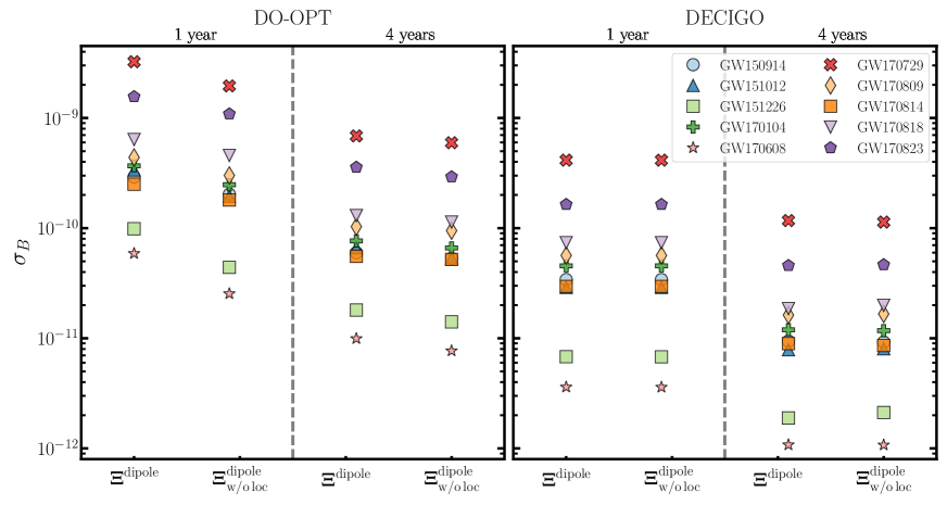
Figure 5: Constraints on the dipole radiation parameter $B$ for all the BBH sources in GWTC-1 for different parameter space sets in the Fisher matrix analysis. Two space-borne detectors, DO-Optimal and DECIGO, are considered. For each detector (panel), the region left / right to the dashed line has an observation duration of 1 year / 4 years. For each column, the label in the abscissa denotes the choice of the parameter set used in the Fisher matrix.

In Table 4 we list the constraints on $B$ that we can obtain from selected ground-based, space-based, and joint observations. We found that space-based constraints are 3–7 orders of magnitude better than ground-based constraints, whereas the best constraint $\sigma_{B}\sim 10^{-12}$ comes from DECIGO. This is caused by the combination of large SNRs and a large number of cycles in the low frequency. Joint observations have a factor of 3–24 further improvement and the best constraint, $\sigma_{B}\sim 3\times 10^{-13}$, comes from the combination of CE and DECIGO. In Fig. 4 we compare the constraints on $\sigma_{B}$ between single-detector observation and joint observation of CE and space-borne detectors. We found that, with the joining of CE, LISA has the most significant improvement, up to a factor of $\sim 24$ for GW150914-like sources; DECIGO has the smallest improvement, about $\sim 3$ for GW170608-like sources.

Among all sources, GW170608 has the lowest redshifted chirp mass, ${\cal M}\sim 8.5\,M_{\odot}$. We notice that once the SNR is high enough, GW170608 always constrains $\sigma_{B}$ better than other BBHs, for BBHs with lower ${\cal M}$ have a lower frequency parameter $u$, which is an advantage in constraining the negative PN order parameter $B$. If we focus our attention on DECIGO and the joint observation of CE and DECIGO, we found that the improvement of joint observation is most significant for heavy systems. For example the improvement is about 9.2 for GW170729-like sources. For light systems like GW170608, only a factor of 3.4 is possible for the improvement. We have also performed calculation for three-detector joint observation and, similarly as before, we conclude that for stellar-mass BBHs the addition of LISA changes the bounds on parameter $B$ very marginally.

For space-based detection, we also investigate the effects from different observation duration, say $T_{\rm obs}=1$ yr versus $T_{\rm obs}=4$ yrs, as well as the effects from different parameter sets, namely $\bm{\Xi}^{\rm dipole}$ and $\bm{\Xi}^{\rm dipole}_{\rm w/o\,loc}$ in Eq. (45) and Eq. (46) respectively. In total we have four combinations of observational scenarios. In Fig. 5 we plot the results for two space-borne detectors, DO-Optimal and DECIGO, respectively in the left and right panels. In each panel, the four cases are divided into two blocks for 1-year observation and 4-year observation. Notice that in each panel, the third column is the same as what was plotted in Fig. 4; the second and fourth columns are the constraints that exclude the consideration of directional parameters in $\bm{\Xi}^{\rm loc}$, as was done by Barausse et al. (2016), Gnocchi et al. (2019), and Carson & Yagi (2020b).

In Fig. 5, comparing the first column with the third column of each panel, we found that the 4-year observation improves the constraints on $B$ by a factor of 4.9 and 3.5 for DO-Optimal and DECIGO respectively. For each detector, comparing the two columns in the 1-year observation scenario and the 4-year observation scenario, we found that the inclusion of sky location worsens the constraints on $B$ in DO-Optimal, but hardly affects the constraints in DECIGO. For DECIGO, because it has 8 detectors, the sky location measurement is already independent of the parameter $B$ measurement, no matter in the 1-year or 4-year observation scenarios. For DO-Optimal, in the 1-year observation scenario, the inclusion of sky location at most worsens the constraints on $\sigma_{B}$ by a factor of 2.3, while in the 4-year observation scenario, it worsens the constraints on $\sigma_{B}$ by a factor of 1.3. Therefore, longer observation could break the degeneracy between directional parameters and the dipole parameter $B$ better. Notice that, with the inclusion of the directional parameters in $\bm{\Xi}^{\rm loc}$, the precision of $B$ for all the sources has similar fractional drops in spite of different SNRs and chirp masses.

5 Discussion

After the first discovery of GWs by the LIGO/Virgo Collaboration with ground-based GW detectors, space-based GW astronomy is guaranteed to trigger a new leap in the field for the next decade. Among the many promising targets, the synergy between ground-based and space-based GW detectors, namely the the multiband observation, will provide unprecedented science ever (Sesana, 2016; Cutler et al., 2019). In this work, we investigate the signal characteristics and parameter estimation for GWTC-1 BBHs with future ground-based and space-based detectors. We show that the multiband observation of CE and space-borne detectors improves the precision of all the considered parameters from a few percent to two orders of magnitude. With its full design and for a 4-year observational time, DECIGO will generate the smallest sky localization area of around $10^{-5}\ \rm arcmin^{2}$ for stellar-mass BBHs. The joint observation of DECIGO and CE gives the best estimation on the parameter precision, while the joint observation of DO-Optimal and CE has the most prominent enhancement, compared to the corresponding space-based observation alone.

The catalog GWTC-1 was used to perform tests of gravity (see e.g. Abbott et al., 2019b; Shao, 2020). We here study the projected constraints on the gravitational dipole radiation in different observation scenarios. Differently from early study, but similarly to a recent one for LISA by Toubiana et al. (2020), we take into consideration of the orbital motion for the space-borne detectors. We found that the best constraint on a generic dimensionless dipole parameter, $\sigma_{B}\sim 10^{-12}$, comes from the joint observation of DECIGO and CE. Finally we compare the bounds on the parameter $B$ with different choices of parameter sets and observational time for DO-Optimal and DECIGO. We conclude that the degeneracy between the directional parameters (including those that characterize the sky location and orbital orientation of the BBH) and the dipole radiation parameter $B$ can be broken by increasing the observational time. This kind of work can be easily extended to other alternative gravity theories within the ppE framework, for examples the Einstein-dilaton-Gauss-Bonnet theory and the dynamical Chern-Simons gravity, as was considered by Gnocchi et al. (2019).

The smaller sky localization area and deeper distance range provided by the multiband observation can help electromagnetic (EM) telescopes with narrow field-of-view to better trace the GW sources (Gehrels et al., 2016). Although stellar-mass BBH systems are generally believed not to have EM counterparts, the follow-up can be used to study some exotic scenarios (see e.g. Ford et al., 2019; Gong et al., 2019). Future multiband and multimessenger observation will enable us to examine the properties of BBHs and BH spacetime in a better way than single detectors can do.

Since the LIGO/Virgo BBH signals in LISA have relatively low SNRs, using ground-based confident detections to identify (in particular sub-threshold) events from space-based observatories is a new avenue for GW detection. Such a reverse tracing can increase event rates by a factor of 4–7 (Wong et al., 2018). This could be a crucial increase for stellar-mass BBH observations with LISA. Furthermore, a more realistic case where the joint observation consists of a space-borne detector and a ground-based detector network (e.g. a network consisting of A+LIGO, CE and ET) could also be considered in future studies (Cutler et al., 2019).

Overall, for stellar-mass BBHs, especially the loudest events among them, multiband observations from millihertz, decihertz to hectohertz will enhance and complement parameter estimation derived solely by space-based or ground-based detection, yield stringent tests of GR, and provide in time the most accurate sky localization. Therefore, multiband detections in future enable us to examine fundamental physics of BHs and gravity theories; meanwhile, with the information of BBH’s population in different GW bands and the possible EM followups, we will better understand the formation and evolution of BBH systems. In a decade time comes the era of multiband GW astronomy and its promising future will deliver due scientific payoff.

Appendix A Parameter estimation in individual GW detectors

In Tables 5 and 6 we list our parameter estimation results for space-based and ground-based GW detectors, respectively.

Table 5: Parameter estimation in GR for LIGO/Virgo BBHs in different space-based GW detectors. We do not list the results for LISA, due to its low SNRs and hence the problem to use the Fisher matrix method.

GW	$\Delta D_{L}/D_{L}$	$\Delta{\cal M}/{\cal M}$	$\Delta\eta/\eta$	$\Delta t_{c}$	$\Delta\phi_{c}$	$\Delta\chi_{1}$	$\Delta\chi_{2}$	$\Delta\Omega$
	(%)	$(10^{-8})$	$(10^{-4})$	(ms)				(${\rm arcmin}^{2}$)
DO-Conservative
GW150914	1.6	3.7	2.2	53	0.065	0.092	0.11	0.80
GW151012	6.1	4.9	4.2	110	0.14	0.12	0.23	15
GW151226	3.7	0.97	1.2	48	0.071	0.070	0.14	1.5
GW170104	3.7	5.4	3.8	100	0.13	0.097	0.16	6.9
GW170608	2.8	0.48	0.72	35	0.058	0.062	0.096	4.5
GW170729	5.0	19	13	380	0.37	0.19	0.30	57
GW170809	3.1	6.0	4.2	120	0.13	0.10	0.17	7.4
GW170814	2.2	3.6	2.3	77	0.082	0.10	0.13	1.8
GW170818	3.5	7.3	5.1	120	0.13	0.16	0.23	8.8
GW170823	5.7	15	11	240	0.26	0.26	0.37	66
DO-Optimal
GW150914	0.82	2.0	0.95	39	0.052	0.029	0.034	0.45
GW151012	3.9	2.6	1.9	67	0.12	0.042	0.080	6.2
GW151226	2.0	0.42	0.49	20	0.048	0.025	0.051	0.32
GW170104	2.0	2.9	1.6	69	0.097	0.024	0.04	3.4
GW170608	1.4	0.22	0.25	13	0.034	0.015	0.023	0.74
GW170729	2.7	12	6.1	280	0.28	0.056	0.090	38
GW170809	1.6	3.4	1.8	89	0.10	0.027	0.043	4.1
GW170814	1.1	2.0	0.99	57	0.066	0.025	0.031	0.93
GW170818	1.9	4.1	2.3	92	0.11	0.048	0.067	4.9
GW170823	4.0	8.8	5.4	190	0.23	0.11	0.15	40
DECIGO
GW150914	0.096	0.23	0.11	0.082	0.0079	0.0038	0.0045	8.6 $\times 10^{-7}$
GW151012	0.47	0.32	0.21	0.31	0.016	0.0038	0.0072	5.4 $\times 10^{-5}$
GW151226	0.30	0.060	0.057	0.21	0.0070	0.0026	0.0052	1.5 $\times 10^{-5}$
GW170104	0.29	0.39	0.22	0.20	0.016	0.0033	0.0055	1.1 $\times 10^{-5}$
GW170608	0.22	0.033	0.031	0.12	0.0050	0.0018	0.0028	5.0 $\times 10^{-5}$
GW170729	0.38	1.5	0.88	0.54	0.047	0.0094	0.015	1.8 $\times 10^{-5}$
GW170809	0.27	0.50	0.30	0.26	0.016	0.0052	0.0083	1.2 $\times 10^{-5}$
GW170814	0.16	0.28	0.15	0.13	0.010	0.0048	0.0060	2.9 $\times 10^{-6}$
GW170818	0.23	0.47	0.27	0.20	0.017	0.0056	0.0079	7.4 $\times 10^{-6}$
GW170823	0.32	0.84	0.49	0.35	0.029	0.0085	0.012	4.7 $\times 10^{-5}$

Table 6: Parameter estimation in GR for LIGO/Virgo BBHs in different ground-based GW detectors.

GW	$\Delta D_{L}/D_{L}$	$\Delta{\cal M}/{\cal M}$	$\Delta\eta/\eta$	$\Delta t_{c}$	$\Delta\phi_{c}$	$\Delta\chi_{1}$	$\Delta\chi_{2}$
	($\%$)	($\%$)	($\%$)	(ms)
AdvLIGO
GW150914	2.0	0.23	2.0	2.5	1.4	0.62	0.74
GW151012	7.3	0.26	11	5.1	4.3	0.48	0.85
GW151226	5.0	0.11	13	2.7	3.2	0.48	0.84
GW170104	5.3	0.36	6.2	5.7	3.3	0.51	0.81
GW170608	3.9	0.084	11	1.6	2.7	0.56	0.80
GW170729	11	2.5	6.8	11	6.9	0.56	0.83
GW170809	4.9	0.46	5.2	6.1	3.2	0.53	0.81
GW170814	3.0	0.24	3.1	2.8	1.9	0.61	0.76
GW170818	4.8	0.51	4.5	4.8	3.2	0.58	0.79
GW170823	7.8	1.1	5.9	6.4	5.3	0.59	0.80
A+LIGO
GW150914	1.0	0.16	1.3	2.3	1.0	0.58	0.68
GW151012	3.6	0.17	6.0	4.6	2.9	0.43	0.77
GW151226	2.4	0.065	7.8	2.4	2.1	0.41	0.74
GW170104	2.6	0.24	3.8	5.1	2.4	0.46	0.73
GW170608	1.9	0.048	6.6	1.4	1.8	0.51	0.74
GW170729	6.0	1.7	4.0	11	5.1	0.55	0.82
GW170809	2.4	0.32	3.3	5.6	2.4	0.48	0.74
GW170814	1.5	0.16	1.9	2.6	1.4	0.57	0.70
GW170818	2.4	0.35	2.7	4.6	2.3	0.55	0.75
GW170823	3.9	0.78	3.3	6.3	3.8	0.58	0.79
CE
GW150914	0.043	0.0023	0.15	0.23	0.013	0.058	0.069
GW151012	0.16	0.0057	0.90	0.72	0.037	0.069	0.12
GW151226	0.11	0.0035	1.3	0.38	0.039	0.069	0.11
GW170104	0.11	0.0045	0.47	0.57	0.029	0.052	0.082
GW170608	0.089	0.0029	1.1	0.26	0.034	0.098	0.13
GW170729	0.19	0.028	0.54	1.7	0.11	0.086	0.13
GW170809	0.10	0.0046	0.38	0.55	0.030	0.049	0.074
GW170814	0.065	0.0029	0.26	0.33	0.017	0.073	0.090
GW170818	0.10	0.0050	0.35	0.55	0.031	0.067	0.091
GW170823	0.16	0.011	0.48	0.98	0.060	0.091	0.13
ET-D
GW150914	0.11	0.0019	0.31	0.54	0.18	0.14	0.16
GW151012	0.42	0.0038	1.5	1.2	0.74	0.11	0.19
GW151226	0.37	0.0029	1.7	0.61	0.80	0.11	0.18
GW170104	0.29	0.0036	0.89	1.2	0.50	0.11	0.17
GW170608	0.33	0.0020	1.3	0.37	0.70	0.13	0.19
GW170729	0.50	0.011	1.1	3.7	0.60	0.18	0.28
GW170809	0.27	0.0039	0.77	1.3	0.43	0.11	0.17
GW170814	0.17	0.0023	0.47	0.67	0.29	0.15	0.18
GW170818	0.26	0.0041	0.72	1.3	0.41	0.16	0.22
GW170823	0.41	0.0070	1.0	2.4	0.55	0.22	0.30

References

- Abbott et al. (2016a) Abbott B. P., et al., 2016a, Phys. Rev. Lett., 116, 061102
- Abbott et al. (2016b) Abbott B. P., et al., 2016b, Astrophys. J., 818, L22
- Abbott et al. (2017) Abbott B. P., et al., 2017, Class. Quant. Grav., 34, 044001
- Abbott et al. (2019a) Abbott B. P., et al., 2019a, Phys. Rev. X, 9, 031040
- Abbott et al. (2019b) Abbott B. P., et al., 2019b, Phys. Rev. D, 100, 104036
- Aghanim et al. (2018) Aghanim N., et al., 2018, arXiv e-prints, p. arXiv:1807.06209
- Amaro-Seoane et al. (2017) Amaro-Seoane P., et al., 2017, arXiv e-prints, p. arXiv:1702.00786
- Arca Sedda et al. (2019) Arca Sedda M., et al., 2019, arXiv e-prints, p. arXiv:1908.11375
- Barack & Cutler (2004) Barack L., Cutler C., 2004, Phys. Rev. D, 69, 082005
- Barausse et al. (2016) Barausse E., Yunes N., Chamberlain K., 2016, Phys. Rev. Lett., 116, 241104
- Barausse et al. (2020) Barausse E., et al., 2020, arXiv e-prints, p. arXiv:2001.09793
- Berti et al. (2005) Berti E., Buonanno A., Will C. M., 2005, Phys. Rev. D, 71, 084025
- Berti et al. (2015) Berti E., et al., 2015, Class. Quant. Grav., 32, 243001
- Berti et al. (2018) Berti E., Yagi K., Yunes N., 2018, Gen. Rel. Grav., 50, 46
- Bohé et al. (2017) Bohé A., et al., 2017, Phys. Rev. D, 95, 044028
- Brans & Dicke (1961) Brans C., Dicke R., 1961, Phys. Rev., 124, 925
- Buonanno & Damour (1999) Buonanno A., Damour T., 1999, Phys. Rev. D, 59, 084006
- Carson & Yagi (2020a) Carson Z., Yagi K., 2020a, Class. Quant. Grav., 37, 02LT01
- Carson & Yagi (2020b) Carson Z., Yagi K., 2020b, Phys. Rev. D, 101, 044047
- Chamberlain & Yunes (2017) Chamberlain K., Yunes N., 2017, Phys. Rev. D, 96, 084039
- Chatziioannou et al. (2019) Chatziioannou K., et al., 2019, Phys. Rev. D, 100, 104015
- Chen & Amaro-Seoane (2017) Chen X., Amaro-Seoane P., 2017, Astrophys. J., 842, L2
- Cutler (1998) Cutler C., 1998, Phys. Rev. D, 57, 7089
- Cutler & Flanagan (1994) Cutler C., Flanagan E. E., 1994, Phys. Rev. D, 49, 2658
- Cutler et al. (2019) Cutler C., et al., 2019, BAAS, 51, 109
- Damour & Esposito-Farèse (1993) Damour T., Esposito-Farèse G., 1993, Phys. Rev. Lett., 70, 2220
- Damour & Esposito-Farèse (1996) Damour T., Esposito-Farèse G., 1996, Phys. Rev. D, 54, 1474
- Fairhurst (2011) Fairhurst S., 2011, Class. Quant. Grav., 28, 105021
- Feng et al. (2019) Feng W.-F., Wang H.-T., Hu X.-C., Hu Y.-M., Wang Y., 2019, Phys. Rev. D, 99, 123002
- Finn (1992) Finn L. S., 1992, Phys. Rev. D, 46, 5236
- Ford et al. (2019) Ford K. E. S., Fraschetti F., Fryer C., Liebling S. L., Perna R., Shawhan P., Veres P., Zhang B., 2019, arXiv e-prints, p. arXiv:1903.11116
- Freire et al. (2012) Freire P. C. C., et al., 2012, Mon. Not. Roy. Astron. Soc., 423, 3328
- Gaebel & Veitch (2017) Gaebel S. M., Veitch J., 2017, Class. Quant. Grav., 34, 174003
- Gehrels et al. (2016) Gehrels N., Cannizzo J. K., Kanner J., Kasliwal M. M., Nissanke S., Singer L. P., 2016, Astrophys. J., 820, 136
- Gerosa et al. (2019) Gerosa D., Ma S., Wong K. W., Berti E., O’Shaughnessy R., Chen Y., Belczynski K., 2019, Phys. Rev. D, 99, 103004
- Gnocchi et al. (2019) Gnocchi G., Maselli A., Abdelsalhin T., Giacobbo N., Mapelli M., 2019, Phys. Rev. D, 100, 064024
- Gong et al. (2019) Gong Y., Cao Z., Gao H., Zhang B., 2019, Mon. Not. Roy. Astron. Soc., 488, 2722
- Hild et al. (2011) Hild S., et al., 2011, Class. Quant. Grav., 28, 094013
- Husa et al. (2016) Husa S., Khan S., Hannam M., Pürrer M., Ohme F., Jiménez Forteza X., Bohé A., 2016, Phys. Rev. D, 93, 044006
- Isoyama et al. (2018) Isoyama S., Nakano H., Nakamura T., 2018, PTEP, 2018, 073E01
- Kawamura et al. (2019) Kawamura S., et al., 2019, Int. J. Mod. Phys. D, 28, 1845001
- Khan et al. (2016) Khan S., Husa S., Hannam M., Ohme F., Pürrer M., Jiménez Forteza X., Bohé A., 2016, Phys. Rev. D, 93, 044007
- Liu et al. (2020) Liu X., Cao Z., Shao L., 2020, Phys. Rev. D, 101, 044049
- Marsat et al. (2020) Marsat S., Baker J. G., Dal Canton T., 2020, arXiv e-prints, p. arXiv:2003.00357
- Moore et al. (2019) Moore C. J., Gerosa D., Klein A., 2019, Mon. Not. Roy. Astron. Soc., 488, L94
- Nair & Tanaka (2018) Nair R., Tanaka T., 2018, JCAP, 1808, 033
- Nair et al. (2016) Nair R., Jhingan S., Tanaka T., 2016, PTEP, 2016, 053E01
- Nishizawa et al. (2016) Nishizawa A., Berti E., Klein A., Sesana A., 2016, Phys. Rev. D, 94, 064020
- Reitze et al. (2019) Reitze D., et al., 2019, BAAS, 51, 141
- Robson et al. (2019) Robson T., Cornish N. J., Liu C., 2019, Class. Quant. Grav., 36, 105011
- Rubbo et al. (2004) Rubbo L. J., Cornish N. J., Poujade O., 2004, Phys. Rev. D, 69, 082003
- Sathyaprakash et al. (2019) Sathyaprakash B., et al., 2019, BAAS, 51, 251
- Sesana (2016) Sesana A., 2016, Phys. Rev. Lett., 116, 231102
- Shao (2020) Shao L., 2020, Phys. Rev. D, 101, 104019
- Shao et al. (2017) Shao L., Sennett N., Buonanno A., Kramer M., Wex N., 2017, Phys. Rev. X, 7, 041025
- Shoemaker (2010) Shoemaker D., 2010, Advanced LIGO anticipated sensitivity curves, https://dcc.ligo.org/cgi-bin/DocDB/ShowDocument?docid=2974
- Tahura et al. (2019) Tahura S., Yagi K., Carson Z., 2019, Phys. Rev. D, 100, 104001
- Taracchini et al. (2012) Taracchini A., et al., 2012, Phys. Rev. D, 86, 024011
- Toubiana et al. (2020) Toubiana A., Marsat S., Barausse E., Babak S., Baker J., 2020, Phys. Rev. D, 101, 104038
- Tso et al. (2019) Tso R., Gerosa D., Chen Y., 2019, Phys. Rev. D, 99, 124043
- Vallisneri (2008) Vallisneri M., 2008, Phys. Rev. D, 77, 042001
- Vitale (2016) Vitale S., 2016, Phys. Rev. Lett., 117, 051102
- Vitale & Whittle (2018) Vitale S., Whittle C., 2018, Phys. Rev. D, 98, 024029
- Wex (2014) Wex N., 2014, in Kopeikin S. M., ed., , Vol. 2, Frontiers in Relativistic Celestial Mechanics: Applications and Experiments. Walter de Gruyter GmbH, Berlin/Boston, p. 39 (arXiv:1402.5594)
- Will (2014) Will C. M., 2014, Living Rev. Rel., 17, 4
- Wong et al. (2018) Wong K. W., Kovetz E. D., Cutler C., Berti E., 2018, Phys. Rev. Lett., 121, 251102
- Yagi & Seto (2011) Yagi K., Seto N., 2011, Phys. Rev. D, 83, 044011
- Yunes & Pretorius (2009) Yunes N., Pretorius F., 2009, Phys. Rev. D, 80, 122003
- Yunes et al. (2016) Yunes N., Yagi K., Pretorius F., 2016, Phys. Rev. D, 94, 084002
- Zhang et al. (2019) Zhang F., Shao L., Zhu W., 2019, Astrophys. J., 877, 87
- Zhao et al. (2019) Zhao J., Shao L., Cao Z., Ma B.-Q., 2019, Phys. Rev. D, 100, 064034