Neutron Star–Neutron Star and Neutron Star–Black Hole Mergers:
Multiband Observations and Early Warnings

Abstract

The detections of gravitational waves (GWs) from binary neutron star (BNS) systems and neutron star–black hole (NSBH) systems provide new insights into dense matter properties in extreme conditions and associated high-energy astrophysical processes. However, currently information about NS equation of state (EoS) is extracted with very limited precision. Meanwhile, the fruitful results from the serendipitous discovery of the $\gamma$-ray burst alongside GW170817 show the necessity of early warning alerts. Accurate measurements of the matter effects and sky location could be achieved by joint GW detection from space and ground. In our work, based on two example cases, GW170817 and GW200105, we use the Fisher information matrix analysis to investigate the multiband synergy between the space-borne decihertz GW detectors and the ground-based Einstein Telescope (ET). We specially focus on the parameters pertaining to spin-induced quadrupole moment, tidal deformability, and sky localization. We demonstrate that, (i) only with the help of multiband observations can we constrain the quadrupole parameter; and (ii) with the inclusion of decihertz GW detectors, the errors of tidal deformability would be a few times smaller, indicating that many more EoSs could be excluded; (iii) with the inclusion of ET, the sky localization improves by about an order of magnitude. Furthermore, we have systematically compared the different limits from four planned decihertz detectors and adopting two widely used waveform models.

1 Introduction

Until now, more than 50 gravitational wave (GW) events have been published by the LIGO/Virgo Collaboration (Abbott et al., 2019a, 2021a, 2021b), in which the majority is from binary black hole (BBH) mergers. In comparison, the GW signals from binary neutron star (BNS) systems (Abbott et al., 2017a, 2020) and neutron star–black hole (NSBH) systems (Abbott et al., 2021c) are rare but of special interests, as they could help us comprehend high-density nuclear matter (Abbott et al., 2018), improve views about astrophysical processes under extreme conditions (Abbott et al., 2017b), and understand compact object populations (Abbott et al., 2021d).

Extracting BNS and NSBH properties solely from GW signals is crucial for GW astronomy, which highly depends on the accuracy of the waveform. Two dominant finite-size effects distinguish NSs from BHs: (i) the deformation due to NS’s own rotation, and (ii) due to the companion’s tidal field. They enter the waveform as self-spin term (Poisson, 1998) and tidal term (Flanagan & Hinderer, 2008; Vines et al., 2011) respectively. With the accurate waveform model (Dietrich et al., 2019a, b), we could constrain the equation-of-state (EoS) dependent spin-induced quadrupole moment and tidal deformability, and pick out the correct EoS model (Read et al., 2009; Hinderer et al., 2010; Agathos et al., 2015), thus informing the low-energy quantum chromodynamics and quark confinement behaviours. Moreover, we could test the nature of BHs (Krishnendu et al., 2019b; Narikawa et al., 2021), distinguish BNS models from BBH models (Chen et al., 2020; Gralla, 2018; Krishnendu et al., 2019a), and test alternative gravity theories (Shao et al., 2017; Sennett et al., 2017; Shao, 2019).

In addition to the GW signal, short $\gamma$-ray burst (GRB), GRB 170817A was found right after the peak of the first BNS inspiral, GW170817 (Abbott et al., 2017a, c). Together with the following counterparts in X-ray, ultraviolet, optical, infrared, and radio bands, simultaneous detections of GWs and electromagnetic (EM) signals initiate a new era of multi-messenger astronomy with precious information (Abbott et al., 2017d). In the meantime, EM signals also call for a better localization ability from GW detectors. Scientists have explored the future localization abilities of LIGO/Virgo detectors (Nitz et al., 2020; Magee et al., 2021), as well as the third generation (3G) detectors including the Europe-led Einstein Telescope (ET; Hild et al., 2011) and the US-led Cosmic Explorer (CE; Abbott et al., 2017e), using the post-Newtonian (PN) waveform (Zhao & Wen, 2018; Chan et al., 2018) with precession (Tsutsui et al., 2021), eccentricity (Ma et al., 2017; Pan et al., 2019), and tidal effects (Wang et al., 2020).

For the discovered LIGO/Virgo sources, the angular resolution of the 3G GW detectors can be as accurate as a few degrees (see e.g., Zhao & Wen, 2018). On the other hand, the space-borne detectors could localize sources within arcminutes (Takahashi & Nakamura, 2003; Nair & Tanaka, 2018). To obtain even better constraints, the multiband observations could be a win-win solution for both space-borne and ground-based detectors.

The BNS and NSBH signals can hardly reach the signal-to-noise ratio (SNR) threshold of the millihertz-band space-borne detectors such as LISA (Amaro-Seoane et al., 2017), and will spend more than a few years before coalescence even if they do. Therefore we direct our attention on the decihertz detectors, e.g., Decihertz Observatories (DOs; Sedda et al., 2020, 2021) and DECihertz laser Interferometer Gravitational wave Observatory (DECIGO; Yagi & Seto, 2011; Kawamura et al., 2019). Because of their shorter arm length, decihertz detectors are sensitive in the frequency range of 0.01–10 Hz. DOs have two LISA-like proposals, the ambitious DO-Optimal and the less challenging DO-Conservative. DECIGO also has two designs. B-DECIGO is a primordial version of DECIGO consisting of one LISA-like detector, while the complete design of DECIGO consists of four independent LISA-like detectors and uses Fabry-Perot cavity to achieve a much lower noise level.

As shown in early studies, the joint detection of BNSs and NSBHs with decihertz detectors and ground-based detectors will improve the parameter precision prominently (Nakamura et al., 2016; Nair et al., 2016; Liu et al., 2020; Nakano et al., 2021). Isoyama et al. (2018) and Nair & Tanaka (2018) have shown the precision improvement specially focusing on BNS finite-size effects and the angular resolution. In this work, we extend the study in Isoyama et al. (2018) by constraining both finite-size effects and localization parameters simultaneously, for both BNS and NSBH systems. Comparing to previous works, we use the updated sensitivity curves and detector designs. For the first time, we give the parameter errors and its multiband improvement distributions on the sky maps. Due to the need of early warnings, we further include multiband sky localization as a function of time. Moreover, our work gives a systematical analysis on parameter correlations, illustrates the capability of different detectors, and compares the implementation of different waveforms. Our work enables a better understanding of joint observations, and could provide more information for different observing scenarios.

In this work, with the help of the Fisher matrix analysis, we investigate the multiband measurement uncertainties considering the complete parameter space including spin, tidal, self spin and location parameters. We give the sky distributions of multiband enhancement for quadrupole-monopole parameters, tidal deformabilities and angular resolutions, as well as the pre-merger localization precision as a function of inspiraling time. We compare the parameter estimation (PE) results of BNS and NSBH systems, using the ET, as a representative of 3G ground-based GW detectors, jointly with a decihertz detector, either from B-DECIGO, DECIGO, DO-Conservative, or DO-Optimal. We adopt both PN and phenomenological waveforms in our study. To be more instructive, we show the projected multiband constraints on NS’s EoS using the limits from tidal deformability. We hope such a detailed study, augmenting the existing investigations, can help researchers lay out the near-future detector science objectives more clearly and understand better about the depth of NS physics that we will learn from such kinds of multiband observations.

The organization of the paper is as follows. In Sec. 2 we introduce the method used in our work, where Sec. 2.1 reviews the NS waveform models; Sec. 2.2 provides the detectors’ configurations and responses; and Sec. 2.3 briefly summarizes the Fisher matrix method and the source properties under study. In Sec. 3 we present our complete PE results, where Sec. 3.1 displays the parameter correlations for BNS and NSBH systems; Sec. 3.2 shows the multiband improvement of quadrupole-monopole parameter, tidal deformability, as well as the differences between BNS and NSBH systems; Sec. 3.3 focuses on limits of extrinsic parameters, especially on the sky localization precision and early warning alerts; Sec. 3.4 compares the PE measurements given by different decihertz detectors; and Sec. 3.5 compares the limits imposed by using PN waveform and phenomenological waveform. In Sec. 4 we discuss constraints on the NS’s EoS, and finally in Sec. 5 we briefly summarize our work. Throughout this paper we use geometrized units in which $G=c=1$.

2 Method

In this section, we first introduce the waveforms used in the following calculations in Sec. 2.1, then we introduce the detectors we use and their responses to GWs in Sec. 2.2, and at last in Sec. 2.3, we briefly summarize the PE method and list the physical properties of the specific example systems that we explore.

2.1 Waveform Construction

We model the GW signal using the Fourier domain, restricted PN approximation (Buonanno et al., 2009). With Fourier representation computed using the stationary phase approximation, the source-frame strain is

$$\tilde{h}_{+}(f) =\mathcal{A}f^{-7/6}e^{i\Psi_{\mathrm{NS}}(f)}\,,$$ (1)

$$\tilde{h}_{\times}(f) =\mathcal{A}f^{-7/6}e^{i[\Psi_{\mathrm{NS}}(f)+\frac{\pi}{2}]}\,,$$ (2)

where the amplitude $\mathcal{A}=\sqrt{{5}/{24}}\pi^{-2/3}{\mathcal{M}^{5/6}}/{D_{L}}$, in which $D_{{L}}$ is the luminosity distance of the source and ${\cal M}=M\eta^{3/5}$ is the chirp mass with the total mass $M=m_{1}+m_{2}$ and the symmetric mass ratio $\eta=m_{1}m_{2}/M^{2}$. Due to the cosmological expansion, we measure the redshifted mass $m_{1,2}=(1+z)\,m_{1,2}^{\rm S}$ of the two compact objects, where $z$ is the redshift calculated from $D_{{L}}$, and $m_{1,2}^{\rm S}$ are the source-frame component masses with $m_{1}^{\rm S}\geq m_{2}^{\rm S}$ by default. Note that we include amplitude’s dependence on the inclination angle in the pattern function (see Sec. 2.2).

The phase $\Psi_{\mathrm{NS}}(f)$ in the waveform is,

$$\Psi_{\mathrm{NS}}(f) =2\pi ft_{\mathrm{c}}-2\phi_{\mathrm{c}}-\frac{\pi}{4}$$

$$+\frac{3}{128\eta v^{5}}\big{(}\Psi_{3.5\,\mathrm{PN}}^{\mathrm{pp}+\mathrm{spin}}+\Psi_{2\mbox{--}3.5\,\mathrm{PN}}^{\mathrm{QM}}+\Psi_{5\mbox{--}6\,\mathrm{PN}}^{\mathrm{tidal}}\big{)}\,,$$ (3)

where $t_{c}$ and $\phi_{c}$ are the time and orbital phase at coalescence, and $v=(\pi Mf)^{1/3}$ is the orbital velocity. Note that terms with ${\cal O}\big{(}v^{2n}\big{)}$ correspond to the $n_{\rm th}$ PN order.

Apart from the BBH baseline waveform, we consider two matter effects specially generated by NSs: the spin-induced and tidal-induced deformations, which respectively count for the second and third terms in the bracket of Eq. (3). In total, the GW phase contains three parts, as elaborated below.

1. The point particle term, $\Psi_{3.5\,\mathrm{PN}}^{\mathrm{pp}+\mathrm{spin}}$ (Arun et al., 2009; Mishra et al., 2016), is kept up to 3.5 PN. Because we consider the non-precessing case, $\Psi_{3.5\,\mathrm{PN}}^{\mathrm{pp}+\mathrm{spin}}$ also contains the aligned spin effect characterized by the dimensionless spin parameters projected to the angular momentum direction, $\chi_{i}=\boldsymbol{S}_{i}\cdot\hat{\boldsymbol{L}}/(m_{i}^{\rm S})^{2}$, where $\boldsymbol{S}_{i}$ is the spin angular momentum and $\hat{\boldsymbol{L}}$ is the unit normal of the orbital plane, expressed later in Eq. (17). $\Psi_{3.5\,\mathrm{PN}}^{\mathrm{pp}+\mathrm{spin}}$ includes the linear spin-orbit effects up to 3.5 PN order, quadratic-in-spin (spin-spin) effects to 3 PN order, and cubic-in-spin (spin-spin-spin) effects to the (leading) 3.5 PN order.

2. The second term is the quadrupole-monopole term, $\Psi_{2\mbox{--}3.5\,\mathrm{PN}}^{\mathrm{QM}}$. The spin-induced quadrupole moment $Q_{i}=-\kappa_{i}\chi_{i}^{2}(m_{i}^{\rm S})^{3}$ is a measure of the degree of the oblateness due to NS’s rotation, where $\kappa_{i}$ is a dimensionless quadrupole parameter with $\kappa_{i}\sim 2\mbox{--}20$ for NSs and $\kappa_{i}=1$ for BHs (Narikawa et al., 2021). This finite size effect that depends on NS’s EoS enters the GW signal as an order-$v^{4}$ correction through the quadrupole-monopole interaction (Poisson, 1998; Mikoczi et al., 2005) and we include them up to 3.5 PN order by (Krishnendu et al., 2017; Nagar et al., 2019; Dietrich et al., 2019a),

   $$\Psi_{2\mbox{--}3.5\,\mathrm{PN}}^{\mathrm{QM}} =-25\tilde{\mathrm{Q}}v^{4}$$

   $$+\bigg{\{}\Big{(}\frac{15635}{42}+60\eta\Big{)}\tilde{\mathrm{Q}}-\frac{2215\delta_{M}}{24}\delta\tilde{\mathrm{Q}}\bigg{\}}v^{6}$$

   $$+\bigg{\{}\Big{[}\frac{375}{2}\left(\chi_{s}+\chi_{a}\delta_{M}\right)-200\pi-10\eta\chi_{s}\Big{]}\tilde{\mathrm{Q}}$$

   $$\quad\quad-\frac{1985}{6}\left(\chi_{a}+\chi_{s}\delta_{M}\right)\delta\tilde{\mathrm{Q}}\bigg{\}}v^{7}\,,$$ (4)

   where

   $$\tilde{Q} =\frac{2m_{1}^{2}\chi_{1}^{2}(\kappa_{1}-1)+2m_{2}^{2}\chi_{2}^{2}(\kappa_{2}-1)}{M^{2}}\,,$$ (5)

   $$\delta\tilde{Q} =\frac{-2m_{1}^{2}\chi_{1}^{2}(\kappa_{1}-1)+2m_{2}^{2}\chi_{2}^{2}(\kappa_{2}-1)}{M^{2}}\,,$$ (6)

   with $\delta_{M}=(m_{1}-m_{2})/M$ and $\chi_{s,a}=(\chi_{1}\pm\chi_{2})/2$. It is $\tilde{Q}$, the combination of individual quadrupole parameters $\kappa_{i}$, to which GW detectors are most sensitive, while $\delta\tilde{Q}$ is the subdominant parameter. We find that, to simultaneously constrain $\kappa_{1}$ and $\kappa_{2}$, or $\tilde{Q}$ and $\delta\tilde{Q}$, is difficult due to the strong degeneracies among the quadrupole parameters and the spin parameters. Therefore we only constrain the leading term $\tilde{Q}$, and we will refer to it as the “quadrupole term” in the following analyses.

3. The last term is the tidal term $\Psi_{5\mbox{--}6\,\mathrm{PN}}^{\mathrm{tidal}}$ (Flanagan & Hinderer, 2008; Vines et al., 2011). At the last stages of the inspiral, the quadrupolar tidal field $\mathcal{E}_{ij}$ of one compact object induces a quadrupole moment ${Q}_{ij}$ to the other component. To the leading order in the adiabatic approximation, ${Q}_{ij}=-\lambda\mathcal{E}_{ij}$ where $\lambda$ is the tidal Love number which takes the form $\lambda(m_{i}^{\rm S},{\rm EoS})=2k_{2}R^{5}(m_{i}^{\rm S})/3$, with $k_{2}$ being the second Love number, and $R(m_{i}^{\rm S})$ is the NS radius as a function of its mass. Both $k_{2}$ and $R(m_{i}^{\rm S})$ are EoS dependent. The deformation effect enters the GW phase from 5 PN through the dimensionless tidal deformability parameter $\Lambda_{i}=\lambda/(m_{i}^{\rm S})^{5}$. We also include the next-to-leading order (6 PN) term (Wade et al., 2014; Narikawa et al., 2021), then

   $$\Psi_{5\mbox{--}6\,\mathrm{PN}}^{\mathrm{tidal}}=-\frac{39}{2}\tilde{\Lambda}v^{10}+\Big{(}-\frac{3115}{64}\tilde{\Lambda}+\frac{6595\delta_{M}}{364}\delta\tilde{\Lambda}\Big{)}v^{12}\,,$$ (7)

   where the combined dimensionless tidal deformabilities $\tilde{\Lambda}$ and $\delta\tilde{\Lambda}$ are

   $$\tilde{\Lambda} =\frac{8}{13}\bigg{[}\Big{(}1+7\eta-31\eta^{2}\Big{)}\left(\Lambda_{1}+\Lambda_{2}\right)$$

   $$+\Big{(}1+9\eta-11\eta^{2}\Big{)}\left(\Lambda_{1}-\Lambda_{2}\right)\delta_{M}\bigg{]}\,,$$ (8)

   $$\delta\tilde{\Lambda} =\frac{1}{2}\bigg{[}\Big{(}1-\frac{13272}{1319}\eta+\frac{8944}{1319}\eta^{2}\Big{)}\left(\Lambda_{1}+\Lambda_{2}\right)\delta_{M}$$

   $$+\Big{(}1-\frac{15910}{1319}\eta+\frac{32850}{1319}\eta^{2}+\frac{3380}{1319}\eta^{3}\Big{)}\left(\Lambda_{1}-\Lambda_{2}\right)\bigg{]}\,.$$ (9)

   Similar to $\tilde{Q}$, the tidal phase is dominated by the leading term characterized by $\tilde{\Lambda}$, and the contribution from $\delta\tilde{\Lambda}$ is small. Hence, we exclude the estimation of $\delta\tilde{\Lambda}$ in our work. We refer to $\tilde{\Lambda}$ as the “tidal deformability” of the system throughout this work. It is worth noting that BHs have zero tidal deformability (Binnington & Poisson, 2009), and for asymmetric NSBHs ($\Lambda_{1}$ = 0, $m_{2}\ll m_{1}$) or very massive BNSs ($\Lambda_{1}$, $\Lambda_{2}\rightarrow 0$), $\tilde{\Lambda}$ will be small and thus they would be indistinguishable from BBHs ($\tilde{\Lambda}$ = 0). For equal mass systems, $\delta\tilde{\Lambda}$=0.

Essentially, in matched filtering, since we do not know the true EoS, we search for the quadrupole parameters and tidal parameters independently. Nevertheless, with the universal Q-Love relations (Yagi & Yunes, 2013, 2017), one can prescribe the quadrupole moments through the tidal deformability without the knowledge of the correct EoS, therefore reducing the number of parameters to infer. Because our purpose is to constrain the EoS, we use $\tilde{Q}$ and $\tilde{\Lambda}$ as separate parameters to estimate. There are waveforms that use the universal relation, such as the phenomenological waveforms (Dietrich et al., 2019b, a), which we will discuss in Sec. 3.5. In that specific section, we will constrain only $\tilde{\Lambda}$.

2.2 Detector Responses and Sensitivities

After having the source-frame waveform in the last subsection, we now construct the detector responses and obtain the detector-frame waveform. For the space-borne detectors, we use the method in Sec. 2.1 of Liu et al. (2020) to model their responses. The basic idea is as follows. The signal received by the detector is

$$\tilde{h}(f) =\Big{[}F^{+}\big{(}f\big{)}\,\tilde{h}_{+}(f)+F^{\times}\big{(}f\big{)}\,\tilde{h}_{\times}(f)\Big{]}e^{-i{\varphi_{D}}(f)}\,,$$ (10)

where the location dependent pattern functions are,

$$F^{+}(\theta,\phi,\psi,\iota) =\frac{\big{(}1+\cos^{2}\iota\big{)}}{2}\ \Big{[}\frac{1}{2}\big{(}1+\cos^{2}\theta\big{)}\cos 2\phi\cos 2\psi-\cos\theta\sin 2\phi\sin 2\psi\Big{]}\,,$$ (11)

$$F^{\times}(\theta,\phi,\psi,\iota) =\cos\iota\ \Big{[}\frac{1}{2}\big{(}1+\cos^{2}\theta\big{)}\cos 2\phi\sin 2\psi+\cos\theta\sin 2\phi\cos 2\psi\Big{]}\,.$$ (12)

The {$\theta,\phi,\psi,\iota$} are the time-varying source direction angles ($\theta$, $\phi$), polarization angle ($\psi$), and inclination angle ($\iota$) in the detector frame. Since we know the orbital motion of the detector, the way to construct the response is to use the fixed {$\bar{\theta}_{S},\bar{\phi}_{S},\bar{\theta}_{L},\bar{\phi}_{L}$}, which are the source direction and angular momentum direction in the Solar system barycentric frame, and the time $t$ to substitute {$\theta,\phi,\psi,\iota$} (see details in Sec. 2 of Liu et al., 2020). The last term of Eq. (10) is the Doppler phase correction (Cutler, 1998),

$$\varphi_{D}(t)={2\pi f}R\sin{\bar{\theta}}_{S}\cos\left[{\Phi_{\rm{space}}}(t)-\bar{\phi}_{S}\right]\,,$$ (13)

where $R=1$ AU is the orbital radius of the detector, and ${\Phi}_{\rm{space}}(t)$ is the azimuthal angle of the detector around the Sun.

The BNS and NSBH signals normally last more than one day in 3G ground-based detectors, so they also have a time-varying $F^{+},F^{\times}$ and $\varphi_{D}$. For ground-based detectors, we follow the same logic as with space-borne detectors to construct their responses. The difference between them is in the transformation from {$\theta,\phi,\psi,\iota$} in Eqs. (11–12) to {$\bar{\theta}_{S},\bar{\phi}_{S},\bar{\theta}_{L},\bar{\phi}_{L},t\}$, which is determined by the detector orbits.

Ground-based detectors rotate with the Earth. We define the latitude of the detector $\delta$, the inclination of Earth’s equator with respect to the ecliptic plane $\epsilon=23^{\circ}26^{\prime}$, the length of a sidereal day $T_{E}$. The Earth’s self rotation phase is ${\Phi}_{\rm{g}}(t)={2\pi t}/{T_{E}}+{\Phi}_{0}$, where ${\Phi}_{0}$ is the initial phase. By assuming that one arm $\hat{\bm{x}}$ points to the south and the other arm $\hat{\bm{y}}$ points to the east, then the unit detector frame $\hat{\bm{x}}$-$\hat{\bm{y}}$-$\hat{\bm{z}}$ in ecliptic coordinate is

$$\hat{\boldsymbol{x}} =\Big{(}\sin\delta\cos\Phi_{\rm{g}}(t),~{}\sin\delta\sin\Phi_{\rm{g}}(t)\cos\epsilon-\cos\delta\sin\epsilon,~{}-\sin\delta\sin\Phi_{\rm{g}}(t)\sin\epsilon-\cos\delta\cos\epsilon\Big{)}\,,$$ (14)

$$\hat{\boldsymbol{y}} =\Big{(}-\sin\Phi_{\rm{g}}(t),~{}\cos\Phi_{\rm{g}}(t)\cos\epsilon,~{}-\cos\Phi_{\rm{g}}(t)\sin\epsilon\Big{)}\,,$$ (15)

$$\hat{\boldsymbol{z}} =\Big{(}\cos\delta\cos\Phi_{\rm{g}}(t),~{}\cos\delta\sin\Phi_{\rm{g}}(t)\cos\epsilon+\sin\delta\sin\epsilon,~{}-\cos\delta\sin\Phi_{\rm{g}}(t)\sin\epsilon+\sin\delta\cos\epsilon\Big{)}\,,$$ (16)

in which $\hat{\boldsymbol{z}}$ points from the Earth center to the detector. Note that, the arm direction could alter, with a rotation angle $\alpha_{0}$, which describes the initial orientation of the detector arms. Together with the the unit vector,

$$\hat{\boldsymbol{L}}=\left(\sin\bar{\theta}_{L}\cos\bar{\phi}_{L},~{}\sin\bar{\theta}_{L}\sin\bar{\phi}_{L},~{}\cos\bar{\theta}_{L}\right)\,,$$ (17)

which is the direction of orbital angular momentum of the source, and the unit vector,

$$\hat{\boldsymbol{N}}=\left(\sin\bar{\theta}_{S}\cos\bar{\phi}_{S},~{}\sin\bar{\theta}_{S}\sin\bar{\phi}_{S},~{}\cos\bar{\theta}_{S}\right)\,,$$ (18)

which is the source’s line-of-sight direction, we have $\cos\theta=\hat{\boldsymbol{N}}\cdot\hat{\boldsymbol{z}}$, $\cos\iota=\hat{\boldsymbol{N}}\cdot\hat{\boldsymbol{L}}$, and

$$\phi =\arctan\left(\frac{\hat{\boldsymbol{N}}\cdot\hat{\boldsymbol{y}}}{\hat{\boldsymbol{N}}\cdot\hat{\boldsymbol{x}}}\right)+\alpha_{0}\,,$$ (19)

$$\tan\psi =\frac{\hat{{\boldsymbol{L}}}\cdot\hat{{\boldsymbol{z}}}-(\hat{{\boldsymbol{L}}}\cdot\hat{{\boldsymbol{N}}})(\hat{{\boldsymbol{z}}}\cdot\hat{{\boldsymbol{N}}})}{\hat{{\boldsymbol{N}}}\cdot(\hat{{\boldsymbol{L}}}\times\hat{{\boldsymbol{z}}})}\,.$$ (20)

Plugging them into Eqs. (11–12), we finally derived the ground-based pattern functions.

The Doppler phase, $\varphi_{D}(t)={2\pi f}R_{E}\cos\theta$, contains the information of the time required for the waves to travel from the geocenter to reach the detector (Zhao & Wen, 2018), where $R_{E}$ is the radius of the Earth. We ignore the Doppler effect due to the Earth’s motion around the Sun in the calculation. It turns out that such omission does not affect the localization precision.

In addition, by transforming the ecliptic coordinate to geocentric coordinate, then substituting it into the PyCBC (Nitz et al., 2021) pattern function code, we have cross-checked the validity of our method. Note that in the above we only model the response of rectangular detectors such as the CE. For triangular ones, one needs to multiply $\sqrt{3}/2$ to $F^{+}$ and $F^{\times}$. We have now obtained $F^{+}$, $F^{\times}$, and $\varphi_{D}$ for both space and ground detectors.

To explore multiband enhancement, for the decihertz observatories, we choose four designs, namely B-DECIGO, DECIGO, DO-Conservative, and DO-Optimal, and we use ET as a representative of the hectohertz ground-based detector. Below we give details on the equivalent number of detectors, the geometrical configuration, the frequency ranges and the relevant literature to obtain their noise power spectral density (PSD).

• For DO-Optimal and DO-Conservative, we use two effective detectors, and triangular LISA-like orbits. Their sensitivity curves are taken from Sedda et al. (2020), which we treat as the averaged PSD over $\theta$, $\phi$, $\psi$, and detector numbers. The frequency range is $[f_{\rm{low}},f_{\rm{high}}]=[10^{-3},10]$ Hz.

• For B-DECIGO, we use two effective detectors, and a triangular LISA-like orbit. The sensitivity curve is taken from Eq. (20) of Isoyama et al. (2018), and the frequency range is $[f_{\rm{low}},f_{\rm{high}}]=[10^{-2},100]$ Hz.

• For DECIGO, we use eight effective detectors with four triangular LISA-like interferometers located from one another by 120^∘ separation on their heliocentric orbits. The sensitivity curve is taken from Eq. (5) of Yagi & Seto (2011), and the frequency range is $[f_{\rm{low}},f_{\rm{high}}]=[10^{-3},100]$ Hz.

• For ET, we adopt the final design ET-D, which has three triangular detectors and possibly be placed at Italy; so we set the latitude of ET $\delta=0.7615$. The sensitivity curve is taken from Hild et al. (2011), and the frequency range is $[f_{\rm{low}},f_{\rm{high}}]=[1,10^{4}]$ Hz.

The sky-averaged noise curves of these GW detectors are given in Fig. 1.

Throughout the paper, we mainly study the PE using synergy of B-DECIGO and ET as a fiducial scenario. We will make comparison with the other three space-borne detectors specifically in Sec. 3.4.

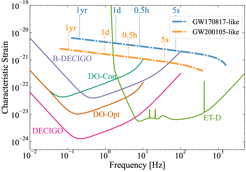
Figure 1: The strain amplitude of the example sources, ${2f|\tilde{h}_{+}(f)|}$, and the characteristic strain of the detector noise, $\sqrt{fS_{n}^{\rm eff}(f)}$, where $S_{n}^{\rm eff}(f)$ is the sky-averaged effective noise defined in Eq. (29) of Liu et al. (2020). Source signals are plotted for a duration of $T_{\rm obs}=4$ yrs. For each source, dashed lines mark the times before coalescence.

2.3 PE Method and Source Selection

We use matched filtering to estimate the binary parameters (Finn, 1992; Cutler & Flanagan, 1994). The noise weighted inner product between two signals, $h(t)$ and $g(t)$, is defined as

$$(h|g)\equiv 2\int_{f_{\rm in}}^{f_{\rm out}}\frac{{\tilde{h}^{*}(f)}\tilde{g}(f)+{\tilde{g}}^{*}(f)\tilde{h}(f)}{S_{n}(f)}{\rm d}f\,,$$ (21)

where ${S_{n}(f)}$ is the noise PSD of the detector; the frequency range ${f_{\rm in}}$ and ${f_{\rm out}}$ are determined by the detector’s limitation and the property of the signal by ${f_{\rm in}}={\rm max}(f_{\rm{4\,yr}},f_{\rm low})$ and ${f_{\rm out}}={\rm min}(f_{\rm{ISCO}},f_{\rm high})$, where $f_{\rm 4\,yr}=\left({t_{\rm obs}}/{5}\right)^{-3/8}{\cal M}^{-5/8}/8\pi$ with $t_{\rm obs}=4\,\rm{yr}$ is the GW frequency 4 years before the merger, and $f_{\rm ISCO}=\left(6^{3/2}\pi M\right)^{-1}$ is the the GW frequency at the innermost stable circular orbit (ISCO) of a Schwarzschild metric with mass $M$. We list $f_{\rm in}$ and $f_{\rm out}$ for different sources in Table 1.

The SNR for a signal $h$ is given by $\rho\equiv\sqrt{(h|h)}$. In the limit of large SNRs, supposing that the noise is stationary and Gaussian, the Fisher matrix method (Finn, 1992) is a fast way to estimate parameter statistical errors. We denote a collection of parameters in a vector, $\bm{\Xi}$. The element of the Fisher matrix $\Gamma_{ab}$ is then given by $\Gamma_{ab}\equiv\left({\partial h}/{\partial\Xi^{a}}\right|\left.{\partial h}/{\partial\Xi^{b}}\right)$, where $h$ is the detector-frame GW strain, i.e. Eq. (10). The error vector, ${\Delta\bm{\Xi}}$, has a multi-variate Gaussian probability distribution (Vallisneri, 2008), $p(\Delta{\bm{\Xi}})\propto\exp\left(-\Gamma_{ab}\Delta\Xi^{a}\Delta\Xi^{b}/2\right)$, where $\Delta\Xi^{a}\equiv\Xi^{a}-\hat{\Xi}^{a}$ with $\hat{\Xi}^{a}$ the maximum-likelihood parameter determined by the matched filtering. The variance-covariance matrix element is given by $\left\langle\delta\Xi^{a}\delta\Xi^{b}\right\rangle=\left(\Gamma^{-1}\right)^{ab}$, then an estimate of the root-mean-square (rms), $\Delta\Xi^{a}$, and the cross-correlation between $\Xi^{a}$ and $\Xi^{b}$, $c^{ab}$, are $\Delta\Xi^{a}=\sqrt{\left(\Gamma^{-1}\right)^{aa}}$ and $c^{ab}={\left\langle\delta\Xi^{a}\delta\Xi^{b}\right\rangle}/{\Delta\Xi^{a}\Delta\Xi^{b}}$, respectively. The angular resolution $\Delta\Omega$ is defined as $\Delta\Omega=2\pi\big{[}\left(\Delta\bar{\mu}_{S}\Delta\bar{\phi}_{S}\right)^{2}-\left\langle\delta\bar{\mu}_{S}\delta\bar{\phi}_{S}\right\rangle^{2}\big{]}^{1/2}$, where $\bar{\mu}_{S}\equiv\cos\bar{\theta}_{S}$ (Lang & Hughes, 2008; Barack & Cutler, 2004). Finally, to estimate parameter precision from joint observations, we add the Fisher matrices from both detectors together via, $\Gamma_{ab}^{\mathrm{joint}}=\Gamma_{ab}^{\mathrm{space}}+\Gamma_{ab}^{\mathrm{ground}}$ (Cutler & Flanagan, 1994).

Table 1: Properties of the GW170817-like BNS system and the GW200105-like NSBH system explored in the paper. We choose a fixed angular momentum direction for both sources for the convenience of later comparison. The fiducial value of $\Lambda_{1}$, $\Lambda_{2}$, $\kappa_{1}$, and $\kappa_{2}$ are set such that their values represent typical NSs and BHs, and the values of $\tilde{Q}$, $\delta\tilde{Q}$, $\tilde{\Lambda}$, and $\delta\tilde{\Lambda}$ are derived using equations in Sec. 2.1.

	GW170817-like	GW200105-like
$m_{1}$ ($M_{\odot}$)	$1.46$	$8.9$
$m_{2}$ ($M_{\odot}$)	$1.27$	$1.9$
$\chi_{1}$	$0.0469$	$0.125$
$\chi_{2}$	$0.002$	$0.004$
$\kappa_{1}$	$9$	$1$
$\kappa_{2}$	$10$	$3$
$\Lambda_{1}$	$675$	$0$
$\Lambda_{2}$	$951$	$237$
$\tilde{\Lambda}$	$793$	$2.81$
$\tilde{Q}$	$1.01\times 10^{-2}$	$1.98\times 10^{-6}$
$\cos\bar{\theta}_{L}$	$-0.65$	$-0.65$
$\bar{\phi}_{L}$ (${\rm rad}$)	$5.016$	$5.016$
$D_{L}$ (Mpc)	$40$	$280$
$z$	$0.01$	$0.06$
$t_{\rm obs,DECIGO/DO}$	4 yr	4 yr
$t_{\rm obs,ET}$	5.6 d	0.90 d
$f_{\rm in,DECIGO/DO}$ (Hz)	0.124	0.0622
$f_{\rm in,ET}$ (Hz)	1.0	1.0
$f_{\rm out,DECIGO}$ (Hz)	100	100
$f_{\rm out,DO}$ (Hz)	10	10
$f_{\rm out,ET}$ (Hz)	1595	384.1

Now we turn to source selection. Because we are interested in both BNS and NSBH systems, we choose our fiducial values from the properties of (i) the BNS inspiral GW170817, and (ii) the NSBH merger GW200105. Meanwhile, we take reasonable values for the poorly measured parameters such as $\chi_{1,2}$, $\kappa_{1,2}$, and $\Lambda_{1,2}$. We list source properties in Table 1. Furthermore, we also select three fixed locations for later comparisons: (I) $\cos\bar{\theta}_{L}=0$ and $\bar{\phi}_{S}=2.0$, (II) $\cos\bar{\theta}_{L}=0.271$ and $\bar{\phi}_{S}=0$, and (III) $\cos\bar{\theta}_{L}=0.936$ and $\bar{\phi}_{S}=4.768$. We will refer to the BNS system at location I/II/III as “BNS I/II/III” and the NSBH analog as “NSBH I/II/III” in the following analyses. As we will see, location I has a large SNR and location III has a precise sky localization.

Finally, we define three parameter sets for the convenience of explication: (i) the intrinsic parameter set,

$$\bm{\Xi}^{\rm int}=\big{\{}{\cal M},\eta,\chi_{s},\tilde{Q},\tilde{\Lambda}\big{\}}\,;$$ (22)

(ii) the extrinsic parameter set

$$\bm{\Xi}^{\rm ext}\equiv\big{\{}t_{c},\phi_{c},D_{L},\bar{\theta}_{S},\bar{\phi}_{S},\bar{\theta}_{L},\bar{\phi}_{L}\big{\}}\,;$$ (23)

and (iii) the localization parameter set which is a subset of $\bm{\Xi}^{\rm ext}$,

$$\bm{\Xi}^{\rm loc}\equiv\big{\{}\bar{\theta}_{S},\bar{\phi}_{S},\bar{\theta}_{L},\bar{\phi}_{L},D_{L}\big{\}}\subset\bm{\Xi}^{\rm ext}\,.$$ (24)

As a short summary, the parameters that we put into the waveforms are,

$$\bm{\Xi}^{\rm input}\equiv\big{\{}m_{1},m_{2},\chi_{1},\chi_{2},\kappa_{1},\kappa_{2},\Lambda_{1},\Lambda_{2}\big{\}}\cup\bm{\Xi}^{\rm ext}\,,$$ (25)

whereas the parameters we estimate are,

$$\bm{\Xi}^{\rm PE}\equiv\bm{\Xi}^{\rm int}\cup\bm{\Xi}^{\rm ext}\,.$$ (26)

For the spin parameters, we choose only to estimate $\chi_{s}$ mainly for two reasons: (i) when simultaneously estimating $\chi_{a}$ and $\chi_{s}$, or $\chi_{1}$, $\chi_{2}$, the correlations between them, as well as with $\tilde{Q}$, become larger than 0.9999 such that the Fisher matrix will be rather singular, while estimating $\chi_{s}$ is slightly uncorrelated than estimating $\chi_{1}$, $\chi_{2}$, or $\chi_{a}$; (ii) from the formation channel point of view, a BNS system often consists of a rapidly spinning, recycled pulsar and a slowly rotating, second-born pulsar whose $\chi$ is very close to zero (Tauris et al., 2017), so estimating one of the spin parameter is sufficient to constrain such a system within an astrophysical setting for field binaries.

It is worth noting that when the contribution of $\delta\tilde{\Lambda}$ grows, the omission of $\delta\tilde{\Lambda}$ in the estimation could lead to over-estimated constraints on $\Delta\tilde{\Lambda}$. On the other hand, the lack of the prior knowledge in our consideration could under-estimate the parameter errors. Quantitatively, we have checked that both kinds of effects on the uncertainties are less than one order of magnitude.

In calculating the Fisher matrix, the analytical expressions for the partial derivative ${\partial\tilde{h}}/{\partial\Xi^{a}}$ are usually not available. We decide to calculate the partial derivatives of $\tilde{h}(f)$ with respect to $t_{c}$, $\phi_{c}$, $\tilde{Q}$, and $\tilde{\Lambda}$ analytically, and calculate the partial derivatives of $\tilde{h}(f)$ with respect to the rest parameters numerically. For the latter, we adopt a numerical scheme that ${\partial\tilde{h}}/{\partial\Xi^{a}}=\tilde{[}h(\Xi^{a}+\delta_{\Xi^{a}})-h(\Xi^{a}-\delta_{\Xi^{a}})]/2\delta_{\Xi^{a}}$, and we have chosen $\delta_{\Xi^{a}}$ for each parameter carefully such that the PE results are stable.

Table 2: The parameter uncertainties of some typical systems. The first two columns label the source type, location and the detectors used. The table is vertically divided into 3 parts, (i) the first part illustrates the effect of different locations for BNSs I, II, and III; (ii) the second part illustrates the effect of different detectors for BNS II; and (iii) the third part illustrates results for NSBH II for comparison with the corresponding BNS results.

System	Detector	SNR	$\Delta{\cal M}/{\cal M}$		$\Delta\eta/\eta$		$\Delta\chi_{s}/\chi_{s}$		$\Delta\tilde{Q}/\tilde{Q}$	$\Delta\tilde{\Lambda}/\tilde{\Lambda}$	$\Delta t_{c}$	$\Delta\phi_{c}$	$\Delta D_{L}/D_{L}$	$\Delta\Omega$
			$(10^{-6})$		$(10^{-3})$		$(10^{-2})$				(ms)	$(10^{-1})$	$(10^{-2})$	$({\rm arcmin}^{2})$
BNS I	ET	1340	0.58	1.5	0.64	1.4	0.0053	0.13	0.11	0.71	2.55 (deg2)
	B-DEC	212	0.023	0.59	4.5	5.6	27	12	5.4	3.3	9.08
	B-DEC+ET	1360	0.0037	0.050	0.18	0.16	0.0040	0.040	0.10	0.49	0.431
BNS II	ET	288	1.9	5.2	2.8	5.2	0.024	0.26	0.23	0.96	0.803 (deg2)
	B-DEC	99.6	0.051	1.2	8.6	10	42	20	9.2	1.0	0.309
	B-DEC+ET	305	0.0092	0.13	0.55	0.49	0.017	0.028	0.14	0.45	0.0128
BNS III	ET	374	1.6	4.4	2.3	4.3	0.019	0.068	0.20	1.2	0.0684 (deg2)
	B-DEC	95.2	0.050	1.2	8.5	10	42	20	9.3	1.7	0.0797
	B-DEC+ET	386	0.0088	0.13	0.51	0.44	0.014	0.023	0.13	0.57	0.00320
BNS II	DO-Con	67.4	0.15	5.2	50	72	3300	300	96	1.5	0.432
	DO-Con+ET	296	0.011	0.17	0.71	0.61	0.018	0.030	0.15	0.49	0.0837
	DO-Opt	406	0.025	0.82	7.9	11	470	44	15	0.25	0.0118
	DO-Opt+ET	498	0.0029	0.053	0.28	0.28	0.016	0.025	0.13	0.21	0.00249
	DECIGO	3240	0.0014	0.040	0.33	0.43	4.1	0.77	0.47	0.031	7.79$\times 10^{-6}$
	DECIGO+ET	3260	0.00060	0.013	0.087	0.097	0.013	0.017	0.070	0.031	7.68$\times 10^{-6}$
NSBH II	ET	105	54	48	5.7	$>10^{5}$	8.7	3.8	3.5	13	184 (deg2)
	B-DEC	36.9	0.3	2.6	5.7	$>10^{4}$	1400	170	11	2.7	32.8
	B-DEC+ET	112	0.079	0.42	0.56	$>10^{3}$	3.3	0.19	0.29	1.2	0.354

Note. — When only ET is used, $\Delta\Omega$ is given in the unit of square degrees.

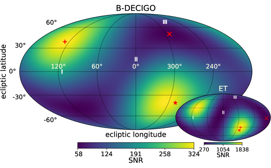
Figure 2: The SNR sky map of BNSs for B-DECIGO (large) and ET (small) in ecliptic coordinate. The red star marks the direction of $\hat{\boldsymbol{L}}$; the red “$\times$” (“$+$”) marks the lowest (highest) SNR in each map. The Roman numbers I, II, and III, mark the source locations I, II, and III. Note that we have used HEALPix^a to help produce the sky maps and the resolution of the map is $\approx 3.4\,{\rm deg^{2}}$. We plot in ecliptic coordinate for all the sky maps in this paper.

^a http://healpix.sf.net

3 Results

In this section, we present our PE results focusing on the constraints of quadrupole parameter, tidal deformability and the localization precision.

We show the dependence of SNR on the source sky position for B-DECIGO and ET respectively in the large and small sky maps in Fig. 2. For the convenience of reading Fig. 2, as well as the following Figs. 4–6, and Fig. 8, we explain the common characteristics of such sky maps here. The plots are based on ecliptic coordinate, showing the signal SNR or PE precision as a function of source’s sky location. The red star in each sky map marks the direction of the source’s angular momentum $\hat{\boldsymbol{L}}$, and the red “$\times/+$” marks the lowest/highest value in each map. The Roman numbers, I, II, and III, mark the source locations I, II, and III.

From Fig. 2 we see that the SNR is larger when the source is either face on or face off, which is intuitive. The slight deviation of the maximum point location is caused by the detector’s orbit. Meanwhile, the minimum point is perpendicular to this direction. In later analyses we show that SNR is not the dominant factor to the PE precision, especially for localization.

We also tabulate the complete PE results in Table 2 for the example sources whose properties are listed in Table 1. It shows the comparison of PE results between different sky locations, different detectors and different systems. We will analyze them in detail in the following subsections.

In Sec. 3.1, we present the parameter correlations from single/joint detection for BNS/NSBH systems. Based on different features of $\bm{\Xi}^{\rm int}$ and $\bm{\Xi}^{\rm ext}$, we analyze the constraints on them respectively in Sec. 3.2 and Sec. 3.3. More specifically, in Sec. 3.2, we show the multiband improvements on $\bm{\Xi}^{\rm int}$, with Sec. 3.2.1 focusing on $\Delta\tilde{Q}$ and Sec. 3.2.2 focusing on $\Delta\tilde{\Lambda}$, and discuss different characteristics of BNS/NSBH systems. In Sec. 3.3, we show the features of $\bm{\Xi}^{\rm ext}$, in which Sec. 3.3.1 investigates the localization ability from space, ground, and multiband observations, and Sec. 3.3.2 displays the evolution of angular resolution with the passing of observing time, which provides information for early warning alerts. In Sec. 3.4, we analyze the different constraints of using DOs/B-DECIGO/DECIGO jointly with ET and in Sec. 3.5, we briefly compare our results with the PE result using another phenomenological waveform, i.e. IMRPhenomPv2_NRTidalv2.

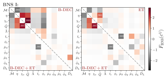
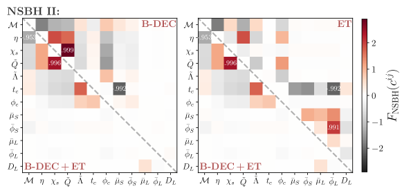
Figure 3: The correlation matrices from the Fisher matrix analysis. The upper (lower) two panels are the parameter correlations for BNS I (NSBH II). In each panel, the upper triangular matrix is for single detectors (B-DEC in the left column and ET in the right column), and the lower triangular matrix is for joint detection (B-DEC+ET). We indicate the name of the detectors in brown in the corresponding corners. The color uses a function, $F(c^{ij})\equiv\log_{10}[(1+c^{ij})/(1-c^{ij})]-c^{ij}\log_{10}2$, adopted from Shao (2016), which is defined such that it counts the number of $9$’s after the decimal point in the cases of large correlations. The largest positive and negative corrections are explicitly given in values for each triangle matrix.

3.1 Parameter Correlations

Figure 3 presents with a specific design the parameter correlations in systems BNS I (upper panels) and NSBH II (lower panels), each with three observing schemes (ET, B-DECIGO, and “B-DECIGO+ET”). We show the correlations between all 12 parameters in $\bm{\Xi}^{\rm PE}$ observed by single detectors in the upper right corners of four panels, with B-DECIGO in the left two panels and ET in the right two panels. We show the joint detection of “B-DECIGO+ET” in the lower left corners in all of four panels with repetition for left and right columns. The shades of the color indicate the degrees of correlation. Intuitively, we see that for both kinds of sources, the boundary between intrinsic parameters $\bm{\Xi}^{\rm int}$ and location parameters $\bm{\Xi}^{\rm loc}$ is evident. The other extrinsic parameters, such as $t_{c}$ and $\phi_{c}$, weakly correlate with both $\bm{\Xi}^{\rm int}$ and $\bm{\Xi}^{\rm loc}$.

Relating the correlation with the PE results in Table 2, we find that the degree of correlation between parameters to some extent indicates the degree of parameter precision one could limit. (i) Space-borne detectors are good at localization, therefore the correlation among the parameters in $\bm{\Xi}^{\rm loc}$ for B-DECIGO is small; see the lower right zone of the B-DECIGO triangular matrix in Fig. 3. ET, on the other hand, has a larger correlation, such as 0.991 between $\bar{\phi}_{S}$ and $\bar{\phi}_{L}$ for the NSBH II system. From the red and black colors of the lower right of two ET triangular matrices we notice that the correlation among the parameters in $\bm{\Xi}^{\rm loc}$ is more obvious in the NSBH II system, since the duration of the NSBH signal in ET is too short to achieve a good localization. (ii) Ground-based detectors are good at constraining intrinsic parameters that enter at high PN orders. This is natural because the high PN terms contribute information largely at the higher frequency band. At the same time, the correlation among parameters in $\bm{\Xi}^{\rm int}$ is smaller than that of B-DECIGO, especially between $\chi_{s}$, $\tilde{Q}$, and $\tilde{\Lambda}$. The correlation between parameters in $\bm{\Xi}^{\rm int}$ and $\bm{\Xi}^{\rm loc}$ is also small for this reason; see the upper rectangle zone of the ET matrices.

In each panel, by comparing the upper triangular matrix with the lower triangular matrix we could see the multiband enhancement. B-DECIGO has large degeneracy between $\chi_{s}$ and $\tilde{Q}$, with $c^{\chi_{s}\tilde{Q}}$ reaching 0.999 in both BNS I and NSBH II systems. Joint detection could lower the correlation to $c^{\chi_{s}\tilde{Q}}=0.997$ for BNS I and $c^{\chi_{s}\tilde{Q}}=0.996$ for NSBH II. ET has large degeneracy among parameters in $\bm{\Xi}^{\rm ext}$, while joint detection could largely reduce this degeneracy. It could even reduce the correlation to nearly zero for the NSBH system.

In Fig. 3, we only show the correlation matrices at locations I and II. However, for sources whose line of sight direction is aligned or anti-aligned with its angular momentum direction, the correlations between $\phi_{c}$ and $\mu_{L}$, as well as between $D_{L}$ and $\phi_{L}$, become larger. They might reach up to 0.9999 and could get even worse in multiband observations. Later we will see that, the red triangles in Fig. 6 and Fig. 8 mark the locations where the maximum correlation of the matrix is larger than 0.9995. For sources in these places, the multiband observations cannot break the degeneracy between parameters in $\bm{\Xi}^{\rm loc}$ at all. Nevertheless, this only happens for these particularly unfavoured, sky locations.

Based on the above arguments, considering the difference between intrinsic and extrinsic parameters, we will analyze them separately in the following two subsections.

3.2 Estimation on Intrinsic Parameters

In this subsection, we illustrate how multiband observations improve intrinsic parameters in $\bm{\Xi}^{\rm int}$, especially focusing on the quadrupole parameter $\tilde{Q}$ and the tidal deformability $\tilde{\Lambda}$. Before digging into them respectively in Sec. 3.2.1 and Sec. 3.2.2, we present some general characteristics first.

Columns (4–8) in Table 2 show the precision of parameters in $\bm{\Xi}^{\rm int}$ for the selected sources. From the first part of the table we find that with the change of location, the parameter precision is approximately inversely proportional to the SNR. But unlike the relation between SNR and distance $D_{L}$, this inverse relation is not exact. For example, using B-DECIGO (ET), the SNR is 2.13 (4.65) times higher at location I than that of location II, but the parameter precision improvement for $\{\Delta{\cal M},\Delta\eta,\Delta\chi_{s},\Delta\tilde{Q},\Delta\tilde{\Lambda}\}$ is {2.17, 2.02, 1.90, 1.84, 1.55} ({3.29, 3.56, 4.31, 3.81, 4.47}) times instead. The deviation of such scaling with SNR indicates the impact of source direction and orientation on estimating parameters in $\bm{\Xi}^{\rm int}$.

During the investigation, we notice that the change of the fiducial values for $\tilde{Q}$ and $\tilde{\Lambda}$ within reasonable ranges will not affect the PE results significantly. In general, with the increasing fiducial values, the estimated errors decrease slightly within an order of magnitude.

We have also verified that all the parameters in $\bm{\Xi}^{\rm int}$ follow the same distribution patterns on sky maps for each detector, similar to those of $\Delta\tilde{Q}$ in Fig. 4 and $\Delta\tilde{\Lambda}$ in Fig. 5. Nevertheless, the precision distribution for extrinsic parameters are different from one another.

In addition, we have executed a Fisher matrix analysis without estimating the localization parameters ($\bar{\phi}_{S},\bar{\theta}_{S}$), which can be seen as the PE precision when the EM counterparts are observed and they provide precise sky location of the sources. We found in that case all errors for parameters in $\bm{\Xi}^{\rm int}$ are about $80\%$ ($99\%$) of the errors in Table 2 for BNS II using B-DECIGO (ET), which is insignificant compared to the improvement of multiband observations with the consideration of localization.

Figure 4: The combined constraints on the quadrupole parameter $\tilde{Q}$ for the BNS system and its multiband improvement compared to a single detector case. See the caption of Fig. 2 for the meanings of marks, including “$\star$”, “$\times$”, “$+$”, and Roman numbers. (a) The combined constraints on $\Delta\tilde{Q}/\tilde{Q}$ using “B-DECIGO+ET”. (b) Large: the improvement of constraining $\Delta\tilde{Q}$ using “B-DECIGO+ET” to B-DECIGO alone; Small: the constraints on $\Delta\tilde{Q}/\tilde{Q}$ using B-DECIGO alone. (c) Large: the improvement of constraining $\Delta\tilde{Q}$ using “B-DECIGO+ET” to ET alone; Small: the constraints on $\Delta\tilde{Q}/\tilde{Q}$ using ET alone.

3.2.1 Quadrupole Parameter

We now focus on the quadrupole parameter, and show how joint detections benefit the observations from space and ground in a mutual way.

In Fig. 4 (a) we show the combined constraints from “B-DECIGO+ET”. The relative error $\Delta\tilde{Q}_{\rm{B+ET}}/\tilde{Q}$ could reach down to 0.1 with the worst cases $<0.8$, which indicates that $\tilde{Q}$ is measurable no matter of the GW source direction. In contrast, the small sky maps in panels (b) and (c) of Fig. 4 reveal that individual observations from neither B-DECIGO nor ET can fully identify this parameter. Comparing the small map in Fig. 4 (c) with Fig. 4 (a), we demonstrate that the sky distribution of the combined precision, $\Delta\tilde{Q}_{\rm{B+ET}}/\tilde{Q}$, as well as other intrinsic parameters as we have verified, is dominated by ET’s distribution pattern, $\Delta\tilde{Q}_{\rm{ET}}/\tilde{Q}$.

The large sky maps in panels (b) and (c) of Fig. 4 stress the multiband effects by plotting the relative improvement in comparison with using B-DECIGO or ET alone. We notice that their distribution patterns are complementary. The colorbar value shows that the joint detection measures 10–50 times better than B-DECIGO alone and 6–12 times better than ET alone. We also notice that the enhancement is less evident (the yellow region) usually at the location where the former detector measures pretty well and the later joined detector measures poorly. There is a small region near the anti-aligned direction of $\hat{\boldsymbol{L}}$ that has a relative lower improvement, which is caused by a degeneracy of location parameters. Such degeneracy gets worse when joining B-DECIGO with ET, therefore it leads to a worse PE improvement (see triangle markers in Fig. 6).

Figure 5: The combined constraints on tidal parameter $\tilde{\Lambda}$, and its multiband improvement compared to the limits from ET alone. See the caption of Fig. 2 for the meanings of marks, including “$\star$”, “$\times$”, “$+$”, and Roman numbers. (a) Large: the combined constraints on $\Delta\tilde{\Lambda}/\tilde{\Lambda}$ for the BNS system using “B-DECIGO+ET”; Small: the improvement of constraining $\Delta\tilde{\Lambda}$ using “B-DECIGO+ET” to ET alone. (b) Large: the combined constraints on $\Delta\tilde{\Lambda}/\tilde{\Lambda}$ for the NSBH system using “B-DECIGO+ET”; Small: the improvement of constraining $\Delta\tilde{\Lambda}$ using “B-DECIGO+ET” to ET alone.

Comparing the distribution of PE errors, e.g. in Fig. 4 (a), with the SNR in Fig. 2, we find the former has larger yellow areas, which also indicates an imperfect inverse relation between PE errors and SNR. Even if some locations have lower SNR, they still yield relative precise PE results.

From the measurement of quadrupole parameter, we see the striking advantage of multiband detection, because $\Delta\tilde{Q}$ determined by a space-borne detector or a ground-based detector alone is too large to yield any constraints, while multiband observations enable pretty good limits on $\Delta\tilde{Q}$.

3.2.2 Tidal Deformability

We now investigate the multiband constraints on the tidal deformability, as well as the comparison between BNS and NSBH systems. In Fig. 5, we show the joint detection errors and multiband enhancement relative to using only ET.

Figure 5 (a) displays the distribution of $\Delta\tilde{\Lambda}_{\rm{B+ET}}/\tilde{\Lambda}$ for the BNS system as a function of sky location, which gives a value ranging between $3\times 10^{-3}$ to $2\times 10^{-2}$. The small sky map indicates that multiband limits are dominated by ET’s value, with 1–2 times tighter when B-DECIGO joins in. In contrast to other intrinsic parameters, the tidal effect starts from 5 PN and contributes largely at the very last stage of inspiral in the ET band, therefore ET plays a leading role in constraining $\tilde{\Lambda}$.

Figure 5 (b) is the NSBH analog to Fig. 5 (a). Comparing the large maps in both panels, we see that the BNS system yields a tighter relative error, $\Delta\tilde{\Lambda}_{\rm{B+ET}}/\tilde{\Lambda}$, while NSBH system can barely measure the tidal deformability, even in the multiband case. To compare them, we select BNS II and NSBH II, and normalize the precision to the same distance $D_{L}$,

$$\Big{[}\frac{\Delta\tilde{\Lambda}_{\rm{B+ET}}}{\tilde{\Lambda}}\Big{]}_{\rm BNS}=0.017\Big{(}\frac{D_{L}}{40\,{\rm Mpc}}\Big{)}\,,$$ (27)

$$\Big{[}\frac{\Delta\tilde{\Lambda}_{\rm{B+ET}}}{\tilde{\Lambda}}\Big{]}_{\rm NSBH}=0.47\Big{(}\frac{D_{L}}{40\,{\rm Mpc}}\Big{)}\,.$$ (28)

Such difference partially comes from the fact that BNS has a larger tidal deformability parameter $\tilde{\Lambda}$, which leads to a larger contribution of the tidal term in the GW phase. The detectors are thus more sensitive to $\tilde{\Lambda}$. Another reason is that BNS signal has a longer time (5.6 d) in ET than NSBH (0.9 d), which helps it accumulate more GW cycles, hence ET could extract more information of the tidal parameter.

The improvement ratio $\Delta\tilde{\Lambda}_{\rm{ET}}/\Delta\tilde{\Lambda}_{\rm{B+ET}}$, on the other hand, is more significant in NSBH system with more information gained from B-DECIGO. From the NSBH II we notice that even when B-DECIGO measures $\Delta\tilde{\Lambda}_{\rm{B}}/\tilde{\Lambda}$ larger than $10^{3}$, in multiband it still helps reduce ET’s uncertainty by about 3 times. Such improvement benefits from the precise measurements of B-DECIGO on other parameters, which helps ET to break the degeneracies among them. It is similar to the measurement of the dipole radiation parameter in Zhao et al. (2021).

The above analysis of comparing BNS and NSBH systems could extend to other parameters as well. For the length of discussion, we do not give too much detail here.

Figure 6: The localization ability of the BNS system. Large: the localization precision improvement using joint detection of “B-DECIGO+ET” than using B-DECIGO alone. Small: localization precision using ET (left) and B-DECIGO (right) alone. The red triangles mark the location where parameter correlations are larger than 0.9995. See the caption of Fig. 2 for the meanings of other marks, including “$\star$”, “$\times$”, “$+$”, and Roman numbers.

3.3 Estimation on Extrinsic Parameters

In this subsection, we demonstrate how multiband observations improve extrinsic parameters in $\bm{\Xi}^{\rm ext}$, especially focusing on the angular resolution $\Delta\Omega$. Same as the last subsection, we begin with some general characteristics of $\bm{\Xi}^{\rm ext}$ and then concentrate respectively in Sec. 3.3.1 and Sec. 3.3.2 on $\Delta\Omega$, and its improvement over time which is important for EM follow-ups.

Worth to note that, in contrast to the intrinsic parameters in $\bm{\Xi}^{\rm int}$, the sky distribution pattern of each parameter in $\bm{\Xi}^{\rm ext}$ is not the same, especially among parameters $D_{L}$, $t_{c}$, $\bar{\phi}_{S}$, and $\bar{\theta}_{S}$, though we only show the distribution of $\Delta\Omega$ in this study.

The time at coalescence $t_{c}$ is an intriguing parameter that correlates with both intrinsic and extrinsic parameters, as can be seen in the correlation matrices in Fig. 3. Therefore measurement of $t_{c}$ will be affected from many aspects. For example, if we know the location of the source from EM observations—which means no need to estimate $\bar{\phi}_{S}$ and $\bar{\theta}_{S}$—unlike $\bm{\Xi}^{\rm int}$, the precision of $t_{c}$ will improve enormously by nearly an order of magnitude. Moreover, although whether or not to include the Earth’s orbit in the Doppler phase $\varphi_{D}(t)$ does not affect the PE results of all other parameters, $\Delta t_{c}$ will be influenced by about one order of magnitude.

Also unlike the nearly inverse relation between intrinsic parameters $\bm{\Xi}^{\rm int}$ and the SNR, the value $\Delta\Omega$ is largely unrelated with SNR. From column (12) in Table 2 we see that among three locations, location I has the largest localization area, but highest SNR. Comparing B-DECIGO’s PE results of BNS II and BNS III, they have similar SNRs, $\Delta\bm{\Xi}^{\rm int}$, $\Delta t_{c}$, and $\Delta\phi_{c}$, but significant differences in $\Delta D_{L}$ and $\Delta\Omega$. The precision $\Delta D_{L}$ is co-determined by the SNR and the sky location of the source.

3.3.1 Sky Localization

Due to the need of an accurate sky location for successful EM follow-ups, we pay close attention to the precision of $\Delta\Omega$. We present the multiband sky localization improvement as well as constraints from individual detectors for the BNS system in Fig. 6. The reason why we display the improvement $\Delta\Omega_{\rm B}/\Delta\Omega_{\rm B+ET}$ other than $\Delta\Omega_{\rm B+ET}$ is that the distribution of $\Delta\Omega_{\rm B+ET}$ is completely dominated by $\Delta\Omega_{\rm B}$’s pattern, which means that the uncertainty distribution of $\Delta\Omega_{\rm B+ET}$ is extremely close to the right small map in Fig. 6. Note that in these sky maps of $\Delta\Omega$, we smooth the values on the map over a few pixels to eliminate the discrete effect caused by a limited number of points. The smoothing leads to a decrease of the maximum value in the B-DECIGO plot, but does not affect the discussions that we have here.

Comparing the two small maps in Fig. 6, we notice that B-DECIGO can localize down to $10^{-2}$ arcmin², which is orders of magnitude better than ET. ET, albeit less powerful, still exceeds most ground-based observatories for it has three individual detectors and a lower cut-off frequency which prolong the signal’s active time in the sensitive band. The localization precisions, as well as sky distributions, are mainly determined by the motions and orbital baselines of the two detectors. The multiband improvement $\Delta\Omega_{\rm B}/\Delta\Omega_{\rm B+ET}$ ranges from $10$ to $50$, which is far better than that of $\Delta\tilde{\Lambda}_{\rm ET}/\Delta\tilde{\Lambda}_{\rm B+ET}$. Considering that both $\Delta\Omega_{\rm ET}$ and $\Delta\tilde{\Lambda}_{\rm B}$ are 3–4 orders of magnitude worse than $\Delta\Omega_{\rm B}$ and $\Delta\tilde{\Lambda}_{\rm ET}$, such a huge improvement in sky localization benefits from the two distinct orbits of B-DECIGO and ET.

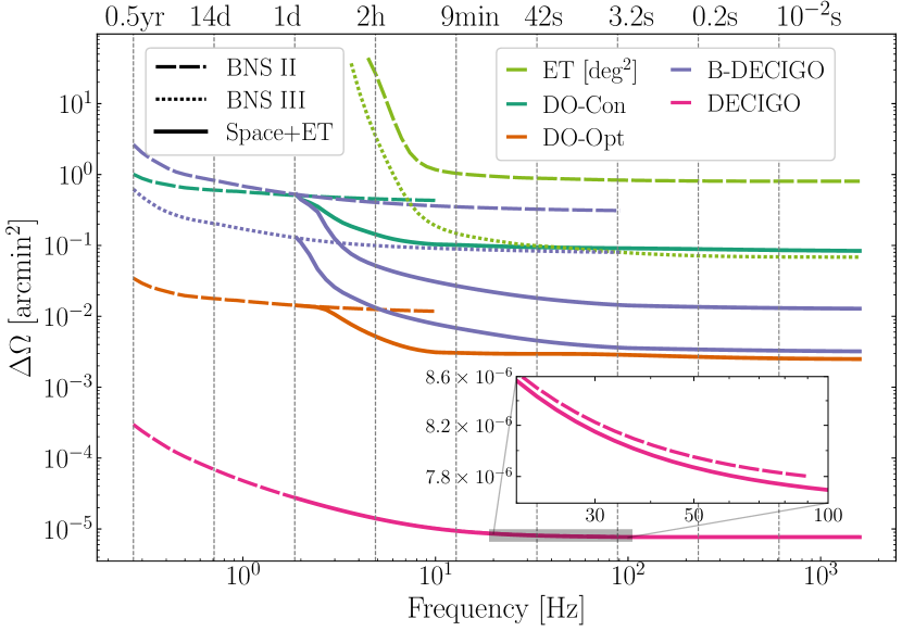
Figure 7: Localization precision $\Delta\Omega$ as a function of frequency (time) for the BNS II and BNS III systems. The dashed (location II) and dotted (location III) lines are the results for single detectors and the solid lines are the results for the joint detection of the corresponding space-borne detectors and ET, which starts from 2 Hz. Note that for ET alone (light green lines), $\Delta\Omega$ is in the unit of square degrees.

From the B-DECIGO plot in the lower right of Fig. 6, we notice large errors in the ecliptic plane. This is a unique effect for the space-borne detectors as it also shows up in Fig. 8 for DOs and DECIGO. Such a phenomenon results from a combination of detector orbits and the signal duration. We first clarify that $\Delta\Omega$ is co-determined by $\Delta\bar{\mu}_{S}$ and $\Delta\bar{\phi}_{S}$, and this “line-like” effect comes from the characteristic of $\bar{\mu}_{S}$.

When the ecliptic polar angle of the source $\bar{\theta}_{S}$ changes from $0^{\circ}/180^{\circ}$ (the two poles) to $90^{\circ}$ (the ecliptic plane), the partial derivative of ${\partial\tilde{h}}/{\partial\bar{\mu}_{S}}$ turns smaller across three orders of magnitude. With the weight $S_{n}$ in Eq. (21), the integral $\Gamma_{\bar{\mu}_{S}\bar{\mu}_{S}}$ becomes smaller by eight orders of magnitude, which makes the error $\Delta\bar{\mu}_{S}$ ranges from $10^{-5}$ to $10^{-2}$ gradually from the two poles to the ecliptic plane. While $\Delta\bar{\phi}_{S}$ stays around $10^{-5}$, the angular resolution is determined by the less accurate $\Delta\bar{\mu}_{S}$; accordingly, large localization errors appear near the ecliptic plane.

However, such “line-like” effect will eventually vanish with the increase of the source masses, thanks to another characteristic from $\bar{\phi}_{S}$. With the increment of mass, GW source merges at a lower frequency, which makes the GW signal exists in the detector’s band for a shorter time—the signal enters the detectors only few months or days before coalescence for decihertz detectors. This is a key factor because ${\partial\tilde{h}}/{\partial\bar{\phi}_{S}}$, which depends strongly on the secular evolution of the detector orbit, is orders of magnitude lower after one month before merger. Without the information of the long-term orbital modulation, the integral $\Gamma_{\bar{\phi}_{S}\bar{\phi}_{S}}$ is tremendously smaller, which leads to a higher $\Delta\bar{\phi}_{S}$. While $\Delta\bar{\mu}_{S}$ still varies greatly with latitude, it no longer dominates the value of $\Delta\Omega$. Therefore the “line-like” effect vanishes.

We have also verified that for sources whose total mass $M\gtrsim 10^{3}M_{\odot}$, this bad measurement along the ecliptic plane disappears. From a mathematic point of view, the whole process is a competition between ${\partial\tilde{h}}/{\partial\bar{\mu}_{S}}$, ${\partial\tilde{h}}/{\partial\bar{\phi}_{S}}$, and $S_{n}$.

We mark the locations, where the maximum correlation in the off-diagonal elements of the correction matrix is over 0.9995, in each map in Fig. 6 by red triangles. We illustrate them briefly in Sec. 3.1 and conclude that ET is slightly better than B-DECIGO in breaking such degeneracy and joint observations deepen this effect by enlarging the regions covered by red triangles.

3.3.2 Early Warnings

Figure 8: The multiband improvement and constraining results of $\Delta\Omega$ [(a) and (b)] and $\Delta\tilde{Q}/\tilde{Q}$ [(c) and (d)] for the BNS system using DO-Optimal [(a) and (c)] and DECIGO [(b) and (d)]. The red triangles mark the location where parameter correlations are larger than 0.9995. See the caption of Fig. 2 for the meanings of other marks, including “$\star$”, “$\times$”, “$+$”, and Roman numbers. (a/b) Large: the improvement of constraining $\Delta\Omega$ using DO-Optimal/DECIGO together with ET to the use of DO-Optimal/DECIGO alone; Small: the constraints on $\Delta\Omega$ using DO-Optimal/DECIGO alone. (c/d) Same as (a/b), for the quadrupole parameter $\tilde{Q}$.

Prompt communication of source location from the GW detection to EM facilities is crucial for multi-messenger follow-ups. While the accurate sky area derived from the complete GW signal is promising, the pre-merger alert is equally important.

We show the localization precision of the BNS systems as a function of frequency in Fig. 7, and mark the time before coalescence at the top of the plot. We find that with the joining in of ET, the localization precision $\Delta\Omega$ gradually narrows. The shape of how $\Delta\Omega$ improves depends on the detectors’ sensitivity curves and designs. In addition, the same shape of the dashed and the dotted blue lines reveals that the location of the source do not affect the variation trend of the multiband improvement.

With nearly 4 years’ time, the space-borne detector already has a stable localization area $\sim\rm{arcmin^{2}}$. ET starts the observation about 5 days before the merger, and it will gradually narrow down its own localization area until a few minutes before merger to be stable, as shown in the light green lines. However, after ET joins the observation, it will not improve the sky area of the space-borne detectors in the first few days. At one day before the merger, the joint detection begins to take effect; $\Delta\Omega$ gradually drops again and finally has an improvement of 1–2 orders of magnitude for DOs and B-DECIGO.

DO-Conservative and B-DECIGO have similar single detector angular resolutions, but different multiband improvements. “B-DECIGO+ET” is about one order of magnitude better than “DO-Conservative+ET”, which is caused by the better sensitivity of B-DECIGO in the high frequency band. Furthermore, from the blue and dark green dashed lines in Fig. 7 we discover that the variation trend of $\Delta\Omega$ with frequency is different: B-DECIGO drops more sharply, despite B-DECIGO and DOs have the same orbital configuration. The reason might be that, at a frequency larger than 0.1 Hz, the BNS signal is at the lowest noise region, the so-called sweet point, of B-DECIGO’s sensitivity curve. Therefore it gains more information from the source after this frequency while DOs get more information before this point.

The multiband enhancement of DECIGO, on the other hand, is different from the other three decihertz detectors. Benefiting from four LISA-like designs, itself can localize precisely to $\sim 10^{-6}~{}\rm{arcmin^{2}}$. The sky area keeps shrinking until minutes before merger and the inclusion of ET barely improves the precision. We will discuss more about comparisons between different decihertz detectors in the next subsection.

3.4 Comparison Between Different Decihertz Detectors

In this subsection, we compare the multiband results by combining ET with different decihertz observatories. In Fig. 8, we plot the DO-Optimal and DECIGO analogs to Fig. 4 (b) and Fig. 6 in order to highlight their similarities and differences.

For the sky localization ability, from the small maps in Fig. 8 (a), Fig. 8 (b), and Fig. 6, we see that the sky distribution is similar, except DECIGO appears more clumpy with more apparent delimitations. DOs have similar designs with B-DECIGO, thus the localization precision is approximately $\propto 1/{\rm SNR}^{2}$. Whereas DECIGO has exceedingly good localization precision down to $10^{-6}\,{\rm arcmin^{2}}$ because of multiple interferometers. This distinction has also been reflected in the large maps in Fig. 8 (a) and Fig. 8 (b), where the difference of multiband enhancement is displayed. From localization point of view, DECIGO’s ability is sufficient by itself.

For intrinsic parameters, based on the measurement on $\Delta\tilde{Q}/\tilde{Q}$, we stress three points. (i) Comparing the small map in Fig. 8 (c) with the small map in Fig. 4 (b), despite DO-Optimal yields larger SNRs, its measurements on $\tilde{Q}$ do not exceed that of B-DECIGO, because DOs have a relatively poor performance at high frequencies. This situation also applies for $\tilde{\Lambda}$ that enters at higher PN order. (ii) Comparing the small map in Fig. 8 (d) with the small map in Fig. 4 (b), we notice that with the help of four interferometers, DECIGO alone could discriminate the quadrupole parameter. Moreover, the uncertainty dispersion on the sky map reduces significantly. (iii) Comparing the large map in Fig. 8 (d) with the small map in Fig. 4 (c), we see that the relative improvement $\Delta\tilde{Q}_{\rm DEC}/\Delta\tilde{Q}_{\rm DEC+ET}$ just follows the distribution of $\Delta\tilde{Q}_{\rm ET}$, which indicates that DECIGO has reached its ceiling in detecting $\Delta\tilde{Q}$.

Figure 9: The $1\,\sigma$ and $2\,\sigma$ constraints from “B-DECIGO+ET” for BNS II using different waveform models.

3.5 Comparison Between Different Waveforms

After investigating the PE results constrained by different detectors, we extend our method to other waveform models and confirm that the PN waveform and phenomenological waveform could yield similar statistical errors.

We adopted two templates implemented in the LIGO Scientific Collaboration (LSC) Algorithm Library (LAL; LIGO Scientific Collaboration, 2018), TaylorF2 and IMRPhenomPv2_NRTidalv2 (Husa et al., 2016; Dietrich et al., 2019a). TaylorF2 is the same with ours except including a tidal correction up to 7 PN. IMRPhenomPv2_NRTidalv2 uses the precessing phenomenological BBH waveform baseline, augmented with a tidal prescription “NRTidalv2”. Other than PN approximation, “NRTidalv2” uses a numerical-relativity-based closed-form tidal phase contribution with a tidal amplitude correction, as well as an inclusion of spin-spin and cubic-in-spin effects up to 3.5 PN (Dietrich et al., 2017, 2019b, 2019a). Furthermore, it implements the universal relations to relate the tidal deformability to the spin-induced quadrupole-monopole terms, and therefore reduces the parameters $\kappa_{1,2}$. To compare our results with it, we change the parameter set to

$$\bm{\Xi}^{\rm PE}\equiv\big{\{}{\cal M},\eta,\chi_{s},\tilde{\Lambda}\big{\}}\cup\bm{\Xi}^{\rm ext}\,,$$ (29)

and inject only the spin-aligned waveforms in IMRPhenomPv2_NRTidalv2.

In Fig. 9, we briefly compare the multiband parameter errors of BNS II detected by “B-DECIGO+ET” adopting “our TaylorF2” in Sec. 2.1, TaylorF2 in LAL, and IMRPhenomPv2_NRTidalv2. We exhibit the results of four parameters $\chi_{s}$, $\tilde{\Lambda}$, $\Delta t_{c}$, and $\phi_{c}$ that vary among the three waveforms. For single-detector detections, such variation is more evident in B-DECIGO and less obvious in ET, and the variation of the combined errors we present here is a mixture of B-DECIGO’s and ET’s trend. We have checked that, the parameters that do not appear in the figure are consistent across all three waveform models. We also find that, without assessing $\tilde{Q}$, $\Delta\Lambda$ has been tightened marginally by 30% than before, from $1.7\%$ to $1.3\%$.

We notice that our lower-order TaylorF2 and TaylorF2 in LAL are very close to each other in the uncertainties and correlations, indicating a weak impact of higher order corrections in this study. In contrast, IMRPhenomPv2_NRTidalv2 gives a wider bound, especially in $\Delta t_{c}$, which may be induced by the complex correlations of $t_{c}$ with other parameters and it also reminds us to be cautious when analyzing $\Delta t_{c}$. The variation in $\Delta\tilde{\Lambda}$ demonstrates that waveform selection has a small impact on statistical errors for the scenarios considered in this paper.

Note that our purpose here is to tentatively compare the statistical errors estimated by the Fisher analysis, which is over-simplified. For detailed analyses on waveform comparison, see Narikawa et al. (2020), Gamba et al. (2021), and Wade et al. (2014).

4 Constraining NS’s EoS

In the above discussion, in particular in Sec. 3.2.2, we have analyzed the projected precision of measuring $\tilde{\Lambda}$. Ultimately, we are interested in limiting individual tidal deformability $\Lambda_{i}$, which relates more closely to the NS’s EoS. Many works have paid attention to it. They have pushed forward the limitation on EoS gradually with more accurate waveforms (Hinderer et al., 2010; Read et al., 2009; Damour et al., 2012), improved Bayesian method (Del Pozzo et al., 2013; Agathos et al., 2015), consideration of a population of BNSs (Lackey & Wade, 2015), and updated detectors (Yagi & Yunes, 2013; Wang et al., 2020). Using the 3G detectors, $\Delta\Lambda_{i}$ can be limited to an accuracy better than 10%.

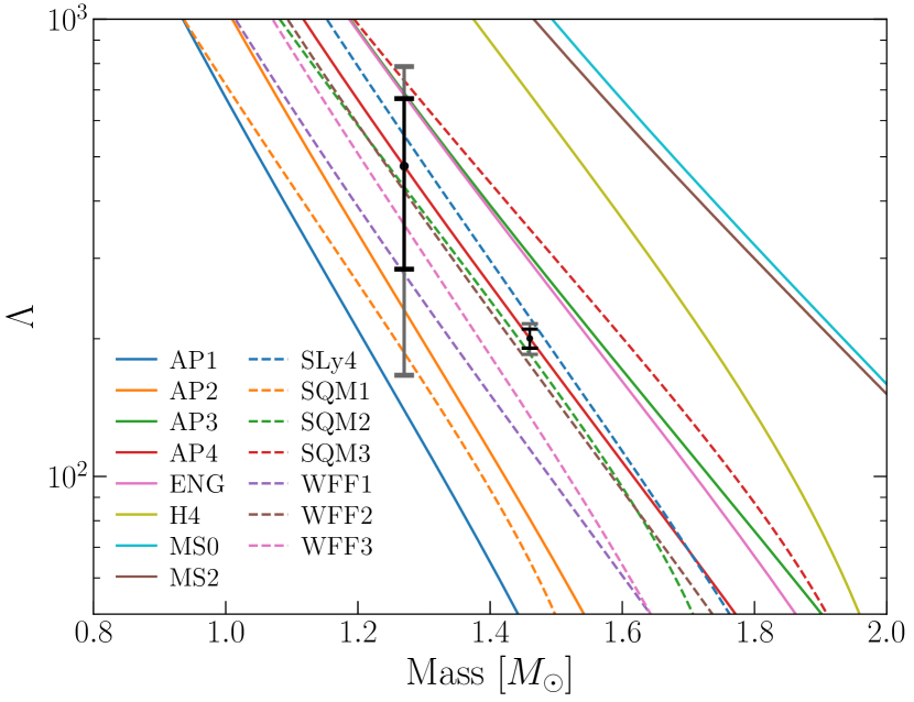
Figure 10: The projected 1 $\sigma$ constraint at $m^{\rm S}_{1}=1.46M_{\odot}$, and the projected 10 $\sigma$ constraint at $m^{\rm S}_{2}=1.27M_{\odot}$, on the individual tidal deformability parameters $\Lambda_{1,2}$ from joint detection using “B-DECIGO+ET” (the black errorbars) versus using ET alone (the grey errorbars). Colored curves give the prediction of $\Lambda$ from different EoSs.

Following early works, we explore the the multiband constraints on $\Lambda_{i}$ here. By Taylor series expanding $\lambda_{i}$ about a fiducial mass $m_{0}^{\rm S}=1.4M_{\odot}$ (Agathos et al., 2015), one gets

$$\lambda_{i}(m)\simeq c_{0}+c_{1}\left(\frac{m^{\rm S}_{i}-m^{\rm S}_{0}}{M_{\odot}}\right)+\frac{1}{2}c_{2}\left(\frac{m_{i}^{\rm S}-m^{\rm S}_{0}}{M_{\odot}}\right)^{2}\,.$$ (30)

We could estimate the precision of $c_{0}$, and then obtain the limitation on $\Lambda_{i}$. We take the EoS AP4 as an example to illustrate the multiband constraints. The fiducial values of $[c_{0},c_{1},c_{2}]$ of AP4 are respectively $[4.09,-3.87,-2.8]\times 10^{-24}\,$s⁵. By assuming that both NSs are described by the same EoS, we use AP4’s tidal deformability as the fiducial values for the BNS system at location II and derive $\Delta\tilde{\Lambda}_{\rm{B+ET}}/\tilde{\Lambda}=4.3\%$ and $\Delta\tilde{\Lambda}_{\rm{ET}}/\tilde{\Lambda}=7.0\%$. Using Eq. (30), we give our multiband constraints on the uncertainty of $\Lambda_{1,2}$,

$$\Delta\Lambda_{1} =19\left(\frac{D_{L}}{40\,{\rm Mpc}}\right)\,,$$ (31)

$$\quad\Delta\Lambda_{2} =10\left(\frac{D_{L}}{40\,{\rm Mpc}}\right)\,.$$ (32)

In Fig. 10 we show the multiband constraints on $\Lambda_{1,2}$. At mass $m^{\rm S}_{1}=1.46\,M_{\odot}$, we plot the 1 $\sigma$ constraints by “B-DECIGO+ET” in black and by ET in grey. We find that joint detection can almost rule out all the wrong EoSs in the plot, while ET alone cannot. To be more illuminative, we show 10 $\sigma$ constraint at mass $m^{\rm S}_{2}=1.27\,M_{\odot}$, which equals to the projected results of such a source but at $\sim$ 10 times further. We find that although many EoSs are within the errorbar, multiband observations eliminate nearly half more of the EoSs than ET alone.

We have to admit that space-borne detector’s help on reducing the errors on $\Lambda$ is not comparable to a reduce in the luminosity distance or a change of source location, as could be seen in Table 2. However, the multiband improvement is a human endeavor other than Nature’s choice about the GW sources. With its help, we are one step closer to understand NS structure and its EoS. In addition, we should be cautious when treating the uncertainties on $\Lambda_{1,2}$, since our assumption is in the limit of $\delta\Lambda\rightarrow 0$, which would break down when the mass ratio of two components grows. In that case an estimation of $\delta\Lambda$ is needed, and if no prior is provided such an estimation will lead to one-order-of-magnitude larger uncertainty on $\Delta\Lambda_{1,2}$. But if some physically motivated prior (e.g., from the universal relation and so on) is included, the effect will not be large. Overall, our result should be viewed as reasonable but optimistic. Meanwhile, as we have carefully checked, the multiband improvement factor basically keeps the same level in both cases, with or without estimating $\delta\Lambda$.

5 Summary

In this paper, we adopted multiband detection strategy, namely using both decihertz GW detectors and the ET, to jointly observe two classes of coalescing binary systems. We take a GW170817-like BNS system and a GW200105-like NSBH system as examples. We analyzed their PE uncertainties, presented the sky distributions of the parameter constraints, and discussed the synergy effects in detail. Here we give a brief summary on our key findings.

1. Assuming the joint B-DECIGO and ET detection and adopting a PN waveform, we found that joint detection could break the strong correlation between the quadrupole parameter and spin parameter, which happens when the source is observed by a decihertz detector alone. The joint detection also breaks the strong correlations among localization parameters which happen when the source is observed by the ET alone.

2. We have showed that only the joint detection could effectively measure the quadrupole parameter for the BNS system. While tidal deformability is detectable by ET alone, joint detection still gives an improvement of a factor of 1–3. Tidal deformability measurements of NSBHs are dozens of times worse than that of BNSs, mainly because NSBHs’ indistinctive tidal contribution to the GW phase.

3. Combining with the EoS information, we constrained the individual tidal deformability and demonstrated that multiband observations could rule out many more EoSs than the use of ET alone, which would greatly help to understand the behaviours of supranuclear dense matters at low temperature.

4. We made comparisons of using different detectors and waveforms. We concluded that DECIGO, made up of 4 independent LISA-like detectors, is remarkably different from the other three space-borne decihertz detectors for its more complex design. We also showed that IMRPhenomPv2_NRTidalv2 waveform constrains the parameters looser than the PN waveform, but the difference is small.

5. BNS systems and some of the NSBH systems are expected to be accompanied with EM counterpart signals. Rapid alerts of source localization are crucial for successful multi-messenger follow-ups for some EM wavebands. We demonstrated that multiband detections could narrow down the arcmin²-level resolution from space-borne decihertz detectors alone by another dozens of times. Meanwhile, joint detections start to take effects about one day before the merger, which makes multiband pre-merger alerts even promising.

In the first three observing runs of the LIGO/Virgo/KAGRA Collaborations, the latencies of public alerts on GW candidates take minutes or hours after the preliminary detection of GW events (Abbott et al., 2019b). With the inclusion of space-borne decihertz detectors, EM facilities can be fore-warned minutes or hours before the merger with an accuracy in sky localization better than a squared arcminute, which, will enable a deeper and more targeted search for the EM counterpart by telescopes with narrow field of view, such as Swift-XRT (Burrows et al., 2005) and JWST (Kalirai, 2018). This hence will maximize the science return in an unprecedented way.

Throughout the paper, priors are ignored in our calculations, or equivalently priors are all considered uniform in each parameter, which leads to under-estimated parameter errors. This can be improved if we have more informed priors from astrophysical or other considerations, for examples, from the limit of Kerr spin in general relativity or the universal relations for NSs. In addition, a full Bayesian analysis could incorporate various kind of prior knowledge and further test effects from different physical priors.

The Fisher information matrix method, which can be viewed as a fast but approximate version of parameter inference, however, has several caveats. It could be problematic when the parameter dimension grows (Harry & Lundgren, 2021), in particular when including complex parameter corrections other than the simple Gaussian ones (Vallisneri, 2008; Smith et al., 2021). In that case, very high correlations might appear and ruin the predictive ability of the Fisher matrix. Though parameters in our parameter set are not highly correlated, the complex relation between intrinsic parameters, for example, between $\tilde{\Lambda}$ and $\delta\tilde{\Lambda}$, still makes us cautious viewing the results. Our analysis is thus only preliminary and indicative. Nevertheless, we have tested our method with the noise curve and system parameters of GW170817, and found consistent results for both tidal deformability and masses with what are reported in the dedicated LIGO/Virgo analysis (Abbott et al., 2017a, 2019c). In addition, we have tested the validity of using the Fisher analysis in our scenarios using the likelihood ratio that was proposed in Vallisneri (2008); we found that the linear signal approximation is satisfied, and the use of Fisher matrix is valid. Moreover, we focus on the statistical errors of the multiband improvement. Nonetheless, such enhancement could be hampered by the systematic errors which result from, e.g. the inaccurate waveform modeling (Isoyama et al., 2018; Gamba et al., 2021). A full Bayesian analysis with consideration of systematic errors will help to address these issues better.

In conclusion, multiband observations of BNS/NSBH systems will complement the single waveband detections in providing new insights into nuclear matters under extreme conditions, origins of high-energy astrophysical phenomena, and so on. We foresee that with future multiband detection, our understanding of astrophysics and fundamental physics will make great progresses and pin down unsolved important puzzles.

References

- Abbott et al. (2017a) Abbott, B. P., et al. 2017a, PhRvL, 119, 161101, doi: 10.1103/PhysRevLett.119.161101
- Abbott et al. (2017b) —. 2017b, ApJL, 850, L39, doi: 10.3847/2041-8213/aa9478
- Abbott et al. (2017c) —. 2017c, ApJL, 848, L13, doi: 10.3847/2041-8213/aa920c
- Abbott et al. (2017d) —. 2017d, ApJL, 848, L12, doi: 10.3847/2041-8213/aa91c9
- Abbott et al. (2017e) —. 2017e, CQGra, 34, 044001, doi: 10.1088/1361-6382/aa51f4
- Abbott et al. (2018) —. 2018, PhRvL, 121, 161101, doi: 10.1103/PhysRevLett.121.161101
- Abbott et al. (2019a) —. 2019a, PhRvX, 9, 031040, doi: 10.1103/PhysRevX.9.031040
- Abbott et al. (2019b) —. 2019b, ApJ, 875, 161, doi: 10.3847/1538-4357/ab0e8f
- Abbott et al. (2019c) —. 2019c, PhRvX, 9, 011001, doi: 10.1103/PhysRevX.9.011001
- Abbott et al. (2020) —. 2020, ApJL, 892, L3, doi: 10.3847/2041-8213/ab75f5
- Abbott et al. (2021a) Abbott, R., et al. 2021a, PhRvX, 11, 021053, doi: 10.1103/PhysRevX.11.021053
- Abbott et al. (2021b) —. 2021b. https://arxiv.org/abs/2108.01045
- Abbott et al. (2021c) —. 2021c, ApJL, 915, L5, doi: 10.3847/2041-8213/ac082e
- Abbott et al. (2021d) —. 2021d, ApJL, 913, L7, doi: 10.3847/2041-8213/abe949
- Agathos et al. (2015) Agathos, M., Meidam, J., Del Pozzo, W., et al. 2015, PhRvD, 92, 023012, doi: 10.1103/PhysRevD.92.023012
- Amaro-Seoane et al. (2017) Amaro-Seoane, P., Audley, H., Babak, S., et al. 2017, arXiv e-prints, arXiv:1702.00786. https://arxiv.org/abs/1702.00786
- Arun et al. (2009) Arun, K. G., Buonanno, A., Faye, G., & Ochsner, E. 2009, PhRvD, 79, 104023, doi: 10.1103/PhysRevD.79.104023
- Barack & Cutler (2004) Barack, L., & Cutler, C. 2004, PhRvD, 69, 082005, doi: 10.1103/PhysRevD.69.082005
- Binnington & Poisson (2009) Binnington, T., & Poisson, E. 2009, PhRvD, 80, 084018, doi: 10.1103/PhysRevD.80.084018
- Buonanno et al. (2009) Buonanno, A., Iyer, B., Ochsner, E., Pan, Y., & Sathyaprakash, B. S. 2009, PhRvD, 80, 084043, doi: 10.1103/PhysRevD.80.084043
- Burrows et al. (2005) Burrows, D. N., et al. 2005, SSRv, 120, 165, doi: 10.1007/s11214-005-5097-2
- Chan et al. (2018) Chan, M. L., Messenger, C., Heng, I. S., & Hendry, M. 2018, PhRvD, 97, 123014, doi: 10.1103/PhysRevD.97.123014
- Chen et al. (2020) Chen, A., Johnson-McDaniel, N. K., Dietrich, T., & Dudi, R. 2020, PhRvD, 101, 103008, doi: 10.1103/PhysRevD.101.103008
- Cutler (1998) Cutler, C. 1998, PhRvD, 57, 7089, doi: 10.1103/PhysRevD.57.7089
- Cutler & Flanagan (1994) Cutler, C., & Flanagan, E. E. 1994, PhRvD, 49, 2658, doi: 10.1103/PhysRevD.49.2658
- Damour et al. (2012) Damour, T., Nagar, A., & Villain, L. 2012, PhRvD, 85, 123007, doi: 10.1103/PhysRevD.85.123007
- Del Pozzo et al. (2013) Del Pozzo, W., Li, T. G. F., Agathos, M., Van Den Broeck, C., & Vitale, S. 2013, PhRvL, 111, 071101, doi: 10.1103/PhysRevLett.111.071101
- Dietrich et al. (2017) Dietrich, T., Bernuzzi, S., & Tichy, W. 2017, PhRvD, 96, 121501, doi: 10.1103/PhysRevD.96.121501
- Dietrich et al. (2019a) Dietrich, T., Samajdar, A., Khan, S., et al. 2019a, PhRvD, 100, 044003, doi: 10.1103/PhysRevD.100.044003
- Dietrich et al. (2019b) Dietrich, T., et al. 2019b, PhRvD, 99, 024029, doi: 10.1103/PhysRevD.99.024029
- Finn (1992) Finn, L. S. 1992, PhRvD, 46, 5236, doi: 10.1103/PhysRevD.46.5236
- Flanagan & Hinderer (2008) Flanagan, E. E., & Hinderer, T. 2008, PhRvD, 77, 021502, doi: 10.1103/PhysRevD.77.021502
- Gamba et al. (2021) Gamba, R., Breschi, M., Bernuzzi, S., Agathos, M., & Nagar, A. 2021, PhRvD, 103, 124015, doi: 10.1103/PhysRevD.103.124015
- Górski et al. (2005) Górski, K. M., Hivon, E., Banday, A. J., et al. 2005, ApJ, 622, 759, doi: 10.1086/427976
- Gralla (2018) Gralla, S. E. 2018, CQGra, 35, 085002, doi: 10.1088/1361-6382/aab186
- Harry & Lundgren (2021) Harry, I., & Lundgren, A. 2021, PhRvD, 104, 043008, doi: 10.1103/PhysRevD.104.043008
- Hild et al. (2011) Hild, S., et al. 2011, CQGra, 28, 094013, doi: 10.1088/0264-9381/28/9/094013
- Hinderer et al. (2010) Hinderer, T., Lackey, B. D., Lang, R. N., & Read, J. S. 2010, PhRvD, 81, 123016, doi: 10.1103/PhysRevD.81.123016
- Husa et al. (2016) Husa, S., Khan, S., Hannam, M., et al. 2016, PhRvD, 93, 044006, doi: 10.1103/PhysRevD.93.044006
- Isoyama et al. (2018) Isoyama, S., Nakano, H., & Nakamura, T. 2018, PTEP, 2018, 073E01, doi: 10.1093/ptep/pty078
- Kalirai (2018) Kalirai, J. 2018, ConPh, 59, 251, doi: 10.1080/00107514.2018.1467648
- Kawamura et al. (2019) Kawamura, S., et al. 2019, IJMPD, 28, 1845001, doi: 10.1142/S0218271818450013
- Krishnendu et al. (2017) Krishnendu, N. V., Arun, K. G., & Mishra, C. K. 2017, PhRvL, 119, 091101, doi: 10.1103/PhysRevLett.119.091101
- Krishnendu et al. (2019a) Krishnendu, N. V., Mishra, C. K., & Arun, K. G. 2019a, PhRvD, 99, 064008, doi: 10.1103/PhysRevD.99.064008
- Krishnendu et al. (2019b) Krishnendu, N. V., Saleem, M., Samajdar, A., et al. 2019b, PhRvD, 100, 104019, doi: 10.1103/PhysRevD.100.104019
- Lackey & Wade (2015) Lackey, B. D., & Wade, L. 2015, PhRvD, 91, 043002, doi: 10.1103/PhysRevD.91.043002
- Lang & Hughes (2008) Lang, R. N., & Hughes, S. A. 2008, ApJ, 677, 1184, doi: 10.1086/528953
- LIGO Scientific Collaboration (2018) LIGO Scientific Collaboration. 2018, LIGO Algorithm Library - LALSuite, doi: 10.7935/GT1W-FZ16
- Liu et al. (2020) Liu, C., Shao, L., Zhao, J., & Gao, Y. 2020, MNRAS, 496, 182, doi: 10.1093/mnras/staa1512
- Ma et al. (2017) Ma, S., Cao, Z., Lin, C.-Y., Pan, H.-P., & Yo, H.-J. 2017, PhRvD, 96, 084046, doi: 10.1103/PhysRevD.96.084046
- Magee et al. (2021) Magee, R., et al. 2021, ApJL, 910, L21, doi: 10.3847/2041-8213/abed54
- Mikoczi et al. (2005) Mikoczi, B., Vasuth, M., & Gergely, L. A. 2005, PhRvD, 71, 124043, doi: 10.1103/PhysRevD.71.124043
- Mishra et al. (2016) Mishra, C. K., Kela, A., Arun, K. G., & Faye, G. 2016, PhRvD, 93, 084054, doi: 10.1103/PhysRevD.93.084054
- Nagar et al. (2019) Nagar, A., Messina, F., Rettegno, P., et al. 2019, PhRvD, 99, 044007, doi: 10.1103/PhysRevD.99.044007
- Nair et al. (2016) Nair, R., Jhingan, S., & Tanaka, T. 2016, PTEP, 2016, 053E01, doi: 10.1093/ptep/ptw043
- Nair & Tanaka (2018) Nair, R., & Tanaka, T. 2018, JCAP, 1808, 033, doi: 10.1088/1475-7516/2018/08/033, 10.1088/1475-7516/2018/11/E01
- Nakamura et al. (2016) Nakamura, T., et al. 2016, PTEP, 2016, 093E01, doi: 10.1093/ptep/ptw127
- Nakano et al. (2021) Nakano, H., Fujita, R., Isoyama, S., & Sago, N. 2021, Univ, 7, 53, doi: 10.3390/universe7030053
- Narikawa et al. (2020) Narikawa, T., Uchikata, N., Kawaguchi, K., et al. 2020, PhRvR, 2, 043039, doi: 10.1103/PhysRevResearch.2.043039
- Narikawa et al. (2021) Narikawa, T., Uchikata, N., & Tanaka, T. 2021, PhRvD, 104, 084056, doi: 10.1103/PhysRevD.104.084056
- Nitz et al. (2021) Nitz, A., Harry, I., Brown, D., et al. 2021, gwastro/pycbc: PyCBC Release 1.18.1, Zenodo, doi: 10.5281/zenodo.4849433
- Nitz et al. (2020) Nitz, A. H., Schäfer, M., & Dal Canton, T. 2020, ApJL, 902, L29, doi: 10.3847/2041-8213/abbc10
- Pan et al. (2019) Pan, H.-P., Lin, C.-Y., Cao, Z., & Yo, H.-J. 2019, PhRvD, 100, 124003, doi: 10.1103/PhysRevD.100.124003
- Poisson (1998) Poisson, E. 1998, PhRvD, 57, 5287, doi: 10.1103/PhysRevD.57.5287
- Read et al. (2009) Read, J. S., Markakis, C., Shibata, M., et al. 2009, PhRvD, 79, 124033, doi: 10.1103/PhysRevD.79.124033
- Sedda et al. (2020) Sedda, M. A., et al. 2020, CQGra, 37, 215011, doi: 10.1088/1361-6382/abb5c1
- Sedda et al. (2021) —. 2021, ExA, 51, 1427, doi: 10.1007/s10686-021-09713-z
- Sennett et al. (2017) Sennett, N., Shao, L., & Steinhoff, J. 2017, PhRvD, 96, 084019, doi: 10.1103/PhysRevD.96.084019
- Shao (2016) Shao, L. 2016, PhRvD, 93, 084023, doi: 10.1103/PhysRevD.93.084023
- Shao (2019) —. 2019, AIP Conf. Proc., 2127, 020016, doi: 10.1063/1.5117806
- Shao et al. (2017) Shao, L., Sennett, N., Buonanno, A., Kramer, M., & Wex, N. 2017, PhRvX, 7, 041025, doi: 10.1103/PhysRevX.7.041025
- Smith et al. (2021) Smith, R., et al. 2021, PhRvL, 127, 081102, doi: 10.1103/PhysRevLett.127.081102
- Takahashi & Nakamura (2003) Takahashi, R., & Nakamura, T. 2003, ApJL, 596, L231, doi: 10.1086/379112
- Tauris et al. (2017) Tauris, T. M., et al. 2017, ApJ, 846, 170, doi: 10.3847/1538-4357/aa7e89
- Tsutsui et al. (2021) Tsutsui, T., Nishizawa, A., & Morisaki, S. 2021, PhRvD, 104, 064013, doi: 10.1103/PhysRevD.104.064013
- Vallisneri (2008) Vallisneri, M. 2008, PhRvD, 77, 042001, doi: 10.1103/PhysRevD.77.042001
- Vines et al. (2011) Vines, J., Flanagan, E. E., & Hinderer, T. 2011, PhRvD, 83, 084051, doi: 10.1103/PhysRevD.83.084051
- Wade et al. (2014) Wade, L., Creighton, J. D. E., Ochsner, E., et al. 2014, PhRvD, 89, 103012, doi: 10.1103/PhysRevD.89.103012
- Wang et al. (2020) Wang, B., Zhu, Z., Li, A., & Zhao, W. 2020, ApJS, 250, 6, doi: 10.3847/1538-4365/aba2f3
- Yagi & Seto (2011) Yagi, K., & Seto, N. 2011, PhRvD, 83, 044011, doi: 10.1103/PhysRevD.83.044011
- Yagi & Yunes (2013) Yagi, K., & Yunes, N. 2013, PhRvD, 88, 023009, doi: 10.1103/PhysRevD.88.023009
- Yagi & Yunes (2017) —. 2017, PhR, 681, 1, doi: 10.1016/j.physrep.2017.03.002
- Zhao et al. (2021) Zhao, J., Shao, L., Gao, Y., et al. 2021, PhRvD, 104, 084008, doi: 10.1103/PhysRevD.104.084008
- Zhao & Wen (2018) Zhao, W., & Wen, L. 2018, PhRvD, 97, 064031, doi: 10.1103/PhysRevD.97.064031
- Zonca et al. (2019) Zonca, A., Singer, L., Lenz, D., et al. 2019, JOSS, 4, 1298, doi: 10.21105/joss.01298