Sequestered Inflation

Abstract

We construct supergravity models allowing to sequester the phenomenology of inflation from the Planckian energy scale physics. The procedure consists of two steps: At Step I we study supergravity models, which might be associated with string theory or M-theory, and have supersymmetric Minkowski vacua with flat directions. At Step II we uplift these flat directions to inflationary plateau potentials. We find certain conditions which ensure that the superheavy fields involved in the stabilization of the Minkowski vacua at Step I are completely decoupled from the inflationary phenomenology.

1 Introduction

Cosmological $\alpha$-attractors Kallosh:2013hoa ; Ferrara:2013rsa ; Kallosh:2013yoa ; Galante:2014ifa are among the very few inflationary models favored by the Planck2018 data Planck:2018jri ; Kallosh:2019hzo . Simplest versions of these models can match all presently available CMB-based observational data by tuning of a single parameter. These models can be implemented in the context of $\mathcal{N}=1$ supergravity, and can be generalized to describe any magnitude of supersymmetry breaking and any value of the cosmological constant Kallosh:2017wnt ; McDonough:2016der .

The main advantage of this class of models is the stability of the cosmological predictions with respect to even very significant modifications of the inflationary potential; inflationary predictions are mainly determined by geometric properties of the moduli space. The required geometric properties are the same as in many phenomenological $\mathcal{N}=1$ 4D supergravity descriptions of string theory. This suggests that if one finds a way to suppress the effects related to steep string theory potentials hindering the development of inflation, it may provide us with string theory (or M-theory) inspired versions of the cosmological $\alpha$-attractors.

Thus, our goal is to construct supergravity models which rely on the geometric properties of the string theory moduli space, while sequestering the low energy scale phenomenology of inflation from the Planckian energy scale physics associated with string theory or M-theory. This problem is highly non-trivial, because supergravity potentials describing many moduli $T_{i}$ have a lot of mixing terms. Cosmological data suggest that the last 50-60 e-foldings of inflation, which are responsible for the formation of the observable part of the universe, occurred at an energy density that is less than $2\times 10^{-9}$ of the Planck density Linde:2016hbb . Thus one may expect that only some symmetries may protect inflation from being affected by the Planckian energy scale physics. Various ideas of symmetries protecting the flatness of the inflationary potential were studied for a long time in string theory and supergravity, see for example Gaillard:1986 ; Gaillard:1995az ; Ellis:2020lnc and Silverstein:2008sg ; Baumann:2010ys ; Baumann:2010nu ; Dong:2010in ; McAllister:2014mpa and references therein.

In this paper we will discuss some models which have supersymmetric Minkowski vacua with flat directions protected by shift symmetries. We will describe a procedure of uplifting these flat directions which preserves their flatness at large values of the moduli and allows to implement $\alpha$-attractors in this context.

This procedure consists of two steps: At Step I we use 4D supergravity with $K^{(I)},W^{(I)}$ and some number of chiral multiplets $T_{i}$ and find string inspired superpotentials such that the scalar potentials have supersymmetric Minkowski vacua with flat directions. This requirement is satisfied for any Kähler potential if the superpotential $W(T_{i})$ and its derivatives $\partial_{j}W(T_{i})$ vanish along some direction.

At Step II we add some $K^{(II)},W^{(II)}$ that uplift these flat directions to inflationary plateau potentials. We find certain conditions which ensure that the superheavy fields, which are involved in the stabilization of the Minkowski vacua at Step I, do not affect inflation. Note that the choice of inflationary potentials here is purely phenomenological, we do not derive them from string theory. However, an important property of $\alpha$-attractors is the stability of their most important predictions with respect to the choice of inflationary potentials. Therefore, we hope that this approach has some merits.

This method was already used in Gunaydin:2020ric for constructing inflationary models in M-theory. However, this was part of a large paper relying on the use of technical tools specific for M-theory. Meanwhile the main idea of our method is quite general, and it is not limited to M-theory, string theory, or $\alpha$-attractors. In this paper, we will explain and generalize this approach, giving some simple examples to illustrate the general idea of protecting the low energy scale phenomenology of inflation from the Planckian energy scale physics.

2 Single field models

2.1 Step I

Consider a model of $n$ chiral superfields $T_{i}$ with a superpotential $W^{(I)}(T_{i})$ (the superpotential at Step I) and with a Kähler potential given by some real holomorphic function $K^{(I)}(T_{i},\overline{T}_{i})$. If at some point $T_{i}=t_{i}+{\rm i}a_{i}$ the superpotential $W^{(I)}(T_{i})$ and all of its first derivatives vanish,

$$W^{(I)}(T_{i})=0\ ,\qquad\partial_{T_{j}}W^{(I)}(T_{i})=0\ ,$$ (1)

this state corresponds to a stable supersymmetric Minkowski vacuum with vanishing scalar potential $V^{(I)}(T_{i})=0$. This property does not depend on the choice of the Kähler potential.

We will be interested in superpotentials such that the conditions (1) are satisfied not only at a single point, but along some flat directions. The potential may have several different flat directions with $V(T_{i})=0$ Gunaydin:2020ric , but the simplest possibility discussed in all examples given in this paper is that the flat direction appears when all fields $T_{i}$ are equal to each other, and real, $T_{i}=t$, $a_{i}=0$.

In this section we will illustrate our general approach using a theory of a single field $T$ with superpotential $W^{(I)}(T)$, for several different choices of the Kähler potential $K^{(I)}(T,\overline{T})$. One should keep in mind that in the theory of a single field supersymmetric flat directions are possible only if $W^{(I)}(T)$ vanishes for all $T$, i.e., if $W^{(I)}(T)=0$. Nevertheless we will keep $W^{(I)}(T)$ in our equations because most of the results to be obtained in this section can be easily generalized for models with many fields $T_{i}$, where flat directions satisfying eqs. (1) may appear for non-trivial superpotentials $W^{(I)}(T_{i})$.

2.1.1 Models with canonical Kähler potential

Consider the model with superpotential $W^{(I)}(T)$ with Kähler potential

$$K^{(I)}(T,\overline{T})=-{1\over 2}(T-\overline{T})^{2}\ .$$ (2)

Now we introduce a nilpotent field $X$, and modify the Kähler potential

$$K^{(II)}=K^{(I)}(T,\overline{T})+{F_{X}^{2}\over F_{X}^{2}+V_{\rm infl}(T,\overline{T})}X\overline{X}\ .$$ (3)

We also modify the superpotential

$$W^{(II)}=W^{(I)}+W_{0}+F_{X}X\ .$$ (4)

In the limit $W_{0}=0$, $F_{X}=0$, and $X=0$ we are back to the model discussed at Step I. Note that Kähler potential $K^{(I)}(T,\overline{T})$ and its first derivatives vanish along its flat direction $T=\overline{T}$

$$\left.K^{(I)}(T,\overline{T})\right|_{{T=\overline{T}}}=0,\qquad\left.{\partial K^{(I)}(T,\overline{T})\over\partial T}\right|_{T=\overline{T}}=\left.{\partial K^{(I)}(T,\overline{T})\over\partial\overline{T}}\right|_{T=\overline{T}}=0\ .$$ (5)

In this case one can show that if $W^{(I)}(T)$ vanishes along the same direction as $K^{(I)}(T,\overline{T})$ (which is trivially satisfied if $W(T)$ vanishes for all $T$), then the potential of the field $T$ for $T=\overline{T}=t$ is given by

$$V_{\rm total}(T)=\left.F_{X}^{2}-3W_{0}^{2}+V_{\rm infl}(T,\overline{T})\right|_{T=\overline{T}=t}\ .$$ (6)

Note that in this expression in the limit $W_{0}=0$, $F_{X}=0$, $V_{\rm infl}=0$, we are back to the model discussed at Step I. Here $F_{X}$ describes the supersymmetry breaking scale and $W_{0}$ corresponds to the gravitino mass. The term $F_{X}^{2}-3W_{0}^{2}$ is the cosmological constant $\Lambda$ at the minimum (if $V_{\rm infl}$ is zero there which will be always the case for us). For the simplest potential $V_{\rm infl}(T,\overline{T})=m^{2}T\overline{T}$ this yields the inflaton potential

$$V_{\rm total}(t)=\Lambda+\frac{1}{2}m^{2}\phi^{2}\ ,$$ (7)

where $\phi=\sqrt{2}t$ is the canonically normalized inflaton. In the context of inflationary cosmology, one may safely use the approximation $\Lambda=0$. The inflaton field $\phi$ has mass squared $m_{\phi}^{2}=m^{2}$. The inflaton trajectory $T=\overline{T}=t\ (=\frac{1}{\sqrt{2}}\phi)$ is stable with respect to the fluctuations in the orthogonal direction $a$, where $T=\frac{1}{\sqrt{2}}(\phi+{\rm i}a)$. Fluctuations of the $a$ field have positive mass squared $m_{a}^{2}=m^{2}(1+\phi^{2})+4W_{0}^{2}$.

Using this method and various potentials $V_{\rm infl}(T,\overline{T})$ one can find many inflationary models consistent with the Planck data. However, the results will be very sensitive to the choice of the potential $V_{\rm infl}(T,\overline{T})$. Therefore, in next sections we will describe $\alpha$-attractors where this issue can be alleviated.

2.1.2 General Kähler potentials

The derivation of the results obtained in the previous subsection required that the Kähler potential $K^{(I)}(T,\overline{T})$ and its first derivatives vanish for $T=\overline{T}$. If this condition is not satisfied, one may use one of the two equivalent methods to be discussed now.

Method 1: One should make a specific Kähler transformation of the Kähler potential $K^{(I)}(T,\overline{T})$ and superpotential $W^{(I)}$ at Step I:

$${\cal K^{(I)}}(T,\overline{T})=K^{(I)}(T,\overline{T})-{\kappa(T)+\kappa(\overline{T})\over 2}\,,\qquad{\cal W^{(I)}}(T)=W^{I}(T)\,e^{\kappa(T)/2}\ ,$$ (8)

where

$$\kappa(T)=K^{(I)}(T,\overline{T})_{|_{\overline{T}\to T}}\ ,\qquad\kappa(\overline{T})=K^{(I)}(T,\overline{T})_{|_{T\to\overline{T}}}\ .$$ (9)

For example, one may start with the simple Kähler potential $K^{(I)}=T\overline{T}$, which is not flat in the direction $T=\overline{T}$. In this case $\kappa(T)=T^{2}$ and $\kappa(\overline{T})=\overline{T}^{2}$. Subtracting ${T^{2}+\overline{T}^{2}\over 2}$ from $K^{(I)}=T\overline{T}$ yields the Kähler potential $-{1\over 2}(T-\overline{T})^{2}$ (2), which has the flat direction $T=\overline{T}$.

The new formulation describes the same theory, with the same flat directions of the superpotential as in the original theory (if there were any), but the Kähler potential in the new formulation satisfies the required flatness conditions (5). Then one can use the same procedure as in the case considered in the previous subsection, with the final result given in eq. (6). This method was used in Gunaydin:2020ric in application to inflation in M-theory.

Method 2: After making these modifications at Step I and adding the term $W_{0}+F_{X}X$ at Step II to the modified superpotential ${\cal W}(T)$, one can perform a reversed Kähler  transformation: multiply the superpotential $W_{I}(T)\,e^{\kappa(T)/2}+W_{0}+F_{X}X$ by $e^{-\kappa(T)/2}$, and make the corresponding transformation of ${\cal K^{(I)}}$. This returns the Kähler potential ${\cal K^{(I)}}$ and the superpotential ${\cal W^{(I)}}(T)$ to their original form $K^{(I)}$ and $W^{(I)}(T)$. The only change which appears after this set of procedures is the modification

$$W_{0}+F_{X}X\qquad\Longrightarrow\qquad(W_{0}+F_{X}X)\,e^{-\kappa(T)/2}$$ (10)

in the expression for $W^{(II)}$ in eq. (4).

The methods 1 and 2 produce equivalent results. We will use the more compact method 2 in the present paper. Namely at Step II we have

$$K^{(II)}(T,\overline{T})=K^{(I)}(T,\overline{T})+{F_{X}^{2}\over F_{X}^{2}+V_{\rm infl}(T,\overline{T})}X\overline{X}\ ,$$ (11)

$$W^{(II)}(T)=W^{(I)}(T)+(W_{0}+F_{X}X)\,e^{-\kappa(T)/2}\ ,$$ (12)

where $\kappa(T)$ is defined in eq. (9). This results in

$$V_{\rm total}(T)=\Lambda+V_{\rm infl}(T,\overline{T})_{|_{T=\overline{T}=t}}\ ,$$ (13)

where $\Lambda=F_{X}^{2}-3W_{0}^{2}$.

In a theory with many fields $T_{i}$ with the Kähler potential given by a sum of independent Kähler potentials for each field $T_{i}$ one should multiply $W_{0}+F_{X}X$ by a product of terms $e^{-\kappa(T_{i})/2}$ for each of the fields $T_{i}$.

In the next subsection we will apply this method to $\alpha$-attractors.

2.1.3 $\alpha$-attractors

Here we will consider a Kähler potential which often appears in $\mathcal{N}=1$ 4D supergravity describing string theory phenomenology. Therefore at Step I we take

$$K^{(I)}(T,\overline{T})=-\log(T+\overline{T}),\qquad W^{(I)}=0\ .$$ (14)

At Step II according to eqs. (11) and (12) we take

$$K^{(II)}(T,\overline{T})=-\log(T+\overline{T})+{F_{X}^{2}\over F_{X}^{2}+V_{\rm infl}(T,\overline{T})}X\overline{X}\ ,$$ (15)

$$W^{(II)}(T)=(W_{0}+F_{X}X)\sqrt{2T}\ ,$$ (16)

since in this model $e^{-\kappa(T)/2}=\sqrt{2T}$. The difference with the previous case is that the field $T$ will have a non-minimal kinetic term. It is convenient to represent the field $T$ as follows:

$$T=e^{-\sqrt{2}\phi}(1+{\rm i}\sqrt{2}a)\ .$$ (17)

The inflaton field $\phi$ is canonical, whereas the field $a$ is also canonical for $a\rightarrow 0$. As an example, one may consider a potential

$$V_{\rm infl}=m^{2}(1-T)(1-\overline{T})\ .$$ (18)

Along the inflaton direction, the total potential is

$$V_{\rm total}(\phi)=\Lambda+m^{2}\left(1-e^{-\sqrt{2}\phi}\right)^{2}\ .$$ (19)

If instead of the Kähler potential (14) one uses the Kähler potential

$$K^{(I)}(T,\overline{T})=-3\alpha\log(T+\overline{T})\ ,$$ (20)

one should use

$$W^{(II)}(T)=(W_{0}+F_{X}X)(2T)^{3\alpha/2}\$$ (21)

to find a family of E-model versions of $\alpha$-attractors with

$$V_{\rm total}(\phi)=\Lambda+m^{2}\left(1-e^{-\sqrt{2\over 3\alpha}\phi}\right)^{2}=\Lambda+m^{2}\left(1-2e^{-\sqrt{2\over 3\alpha}\phi}+...\right)\ .$$ (22)

One can considerably change the potential $V_{\rm infl}(T,\overline{T})$, but the large $\phi$ asymptotic behavior of this potential remains the same, up to a change of the parameter $m^{2}$ and a redefinition (shift) of the canonical field $\phi$. This is the reason why these models are called cosmological attractors. The model (19) describes $\alpha$-attractor with $\alpha=1/3$. In $\mathcal{N}=1$ supergravity $3\alpha$ is an arbitrary parameter defining the moduli space curvature. In the case with an underlying maximal supersymmetry or string/M-theory one may have $3\alpha=7,6,5,4,3,2,1$, see Refs. Ferrara:2016fwe ; Kallosh:2017ced ; Kallosh:2017wnt ; Gunaydin:2020ric .

Instead of $T$ variables with Kähler potential (15) and superpotential (21) describing a half (complex) plane $T+\overline{T}>0$, one can use disk variables $Z=\frac{T-1}{T+1}$ with the resulting Kähler potential

$$K^{(II)}(Z,\overline{Z})=-3\alpha\log(1-Z\overline{Z})+{F_{X}^{2}\over F_{X}^{2}+V_{\rm infl}(Z,\overline{Z})}X\overline{X},$$ (23)

and superpotential

$$W^{(II)}=(W_{0}+F_{X}X)(1-Z^{2})^{3\alpha/2}\ ,$$ (24)

which yields

$$V_{\rm total}(Z)=\Lambda+V_{\rm infl}(Z,\overline{Z})_{|_{Z=\overline{Z}=z}}\ .$$ (25)

For $V_{\rm infl}(Z,\overline{Z})=m^{2}Z\bar{Z}$ (and ignoring $\Lambda$) this leads to a family of T-models with the potential of the canonical inflaton field $\phi$

$$V(\phi)=m^{2}\tanh^{2}{\phi\over\sqrt{6\alpha}}\ ,$$ (26)

where $z=\tanh{\phi\over\sqrt{6\alpha}}$. At $\alpha\ll 1$, E-models (19) and T-models (26) give very similar predictions for the spectral index $n_{s}$ and tensor to scalar ratio $r$ for a given number of e-foldings $N_{e}$:

$$n_{s}=1-{2\over N_{e}},\qquad r={12\alpha\over N_{e}^{2}}\ .$$ (27)

At larger $\alpha$, the predictions of these two families of models slightly differ, see Fig. 1.

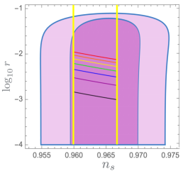
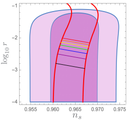
Figure 1: Predictions of the simplest T-models (left) and E-models (right) for $50\leq N_{e}\leq 60$ Kallosh:2019hzo . Red ellipses show the Planck 2018 results taking into account the CMB-related data including data from BICEP2/Keck. String theory motivated versions of these models have 7 specific predictions Ferrara:2016fwe ; Kallosh:2017ced : $3\alpha=7$ (red line), $3\alpha=6$ (orange), $3\alpha=5$ (yellow), $3\alpha=4$ (green), $3\alpha=3$ (blue), $3\alpha=2$ (purple) and $3\alpha=1$ (black). All other values of $\alpha$ originate from general $N=1$ supergravity models.

3 Two field model

3.1 Step I

Now we will study a more advanced model, with two fields $T_{1}$ and $T_{2}$, which have a nontrivial superpotential already at Step I:

$$K^{(I)}=-{1\over 2}\sum_{i=1}^{2}(T_{i}-\overline{T}_{i})^{2}\,,\qquad W^{(I)}=M(T_{1}-T_{2})^{2}\ .$$ (28)

There is a supersymmetric Minkowski vacuum at $T_{1}=T_{2}$. The canonically normalized variables $T_{i}=\frac{1}{\sqrt{2}}(\phi_{i}+{\rm i}a_{i})$ can be rewritten in terms of canonically normalized mass eigenstates as $\phi=\frac{1}{\sqrt{2}}(\phi_{1}+\phi_{2})$, $a=\frac{1}{\sqrt{2}}(a_{1}+a_{2})$, $\phi_{M}=\frac{1}{\sqrt{2}}(\phi_{1}-\phi_{2})$ and $a_{M}=\frac{1}{\sqrt{2}}(a_{1}-a_{2})$. The mass eigenvalues of $\phi,a$ at $T_{1}=T_{2}=0$ are $0$ and the mass eigenvalues of the massive modes $\phi_{M},a_{M}$ at $T_{1}=T_{2}=0$ are $m^{2}=16M^{2}$. This mass is below the Planck mass $M_{Pl}=1$ for $M<{1\over 4}$.

The absence of tensor modes at the level $r\lesssim 0.05$ implies that the inflaton potential $V$ at the last 60 e-foldings of inflation should be smaller than $2\times 10^{-9}$ Linde:2016hbb . This means that if the field $T_{1}+T_{2}=\phi+{\rm i}a$ deviates from its equilibrium at $T_{1}+T_{2}=0$ by $O(1)$, its potential can become many orders of magnitude higher than the inflationary potential $V$. Thus it is necessary to check whether the scenario outlined in the previous section may remain intact despite the introduction of the large superpotential $W^{(I)}=M(T_{1}-T_{2})^{2}$.

3.2 Step II

Just as in the previous section, we introduce a nilpotent field $X$ and modify the Kähler potential and the superpotential

$$K^{(II)} = K^{(I)}+{F_{X}^{2}\over F_{X}^{2}+V_{\rm infl}(T_{i},\overline{T}_{i})}X\overline{X}\ ,$$ (29)

$$W^{(II)} = W^{(I)}+W_{0}+F_{X}X\ .$$ (30)

Fortunately, the Kähler potential $K^{(I)}$ vanishes along the flat direction $T_{1}=\overline{T}_{1}=t$, $T_{2}=\overline{T}_{2}=t$ along which the superpotential $W^{(I)}$ also vanishes. As a result, one can show that eq. (6) derived for the model with $W^{(I)}=0$ remains valid as well. At this time, instead of a simple quadratic scalar potential we will take a more complicated one

$$V_{\rm infl}(T_{i},\overline{T}_{i})={g^{2}|T_{1}|^{2}|T_{2}|^{2}\over\mu^{4}+|T_{1}|^{2}|T_{2}|^{2}}\ .$$ (31)

At $T_{M}=0$ and $T_{i}=\overline{T}_{i}=t$ the potential depends only on the canonical inflaton field $T=\frac{1}{\sqrt{2}}\phi\ (=t)$ and (for $\Lambda=0$) is given by

$$V_{\rm infl}(\phi)=g^{2}{\phi^{4}\over 4\mu^{4}+\phi^{4}}\ .$$ (32)

This is the plateau potential of the D-brane inflation model described recently in Kallosh:2018zsi . It was called KKLTI in the Encyclopedia Inflationaris Martin:2013tda because of its possible relation to the KKLT mechanism of vacuum stabilization and inflation in string theory Kachru:2003aw ; Kachru:2003sx . This model is in good agreement with observational data. Its prediction

$$n_{s}=1-{5\over 3N_{e}}$$ (33)

is very close to the prediction of the $\alpha$-attractors $n_{s}=1-{2\over N_{e}}$. This model and $\alpha$-attractors almost completely cover the area in the $(n_{s},r)$ plane favored by Planck2018 Kallosh:2019hzo , see Fig. 2.

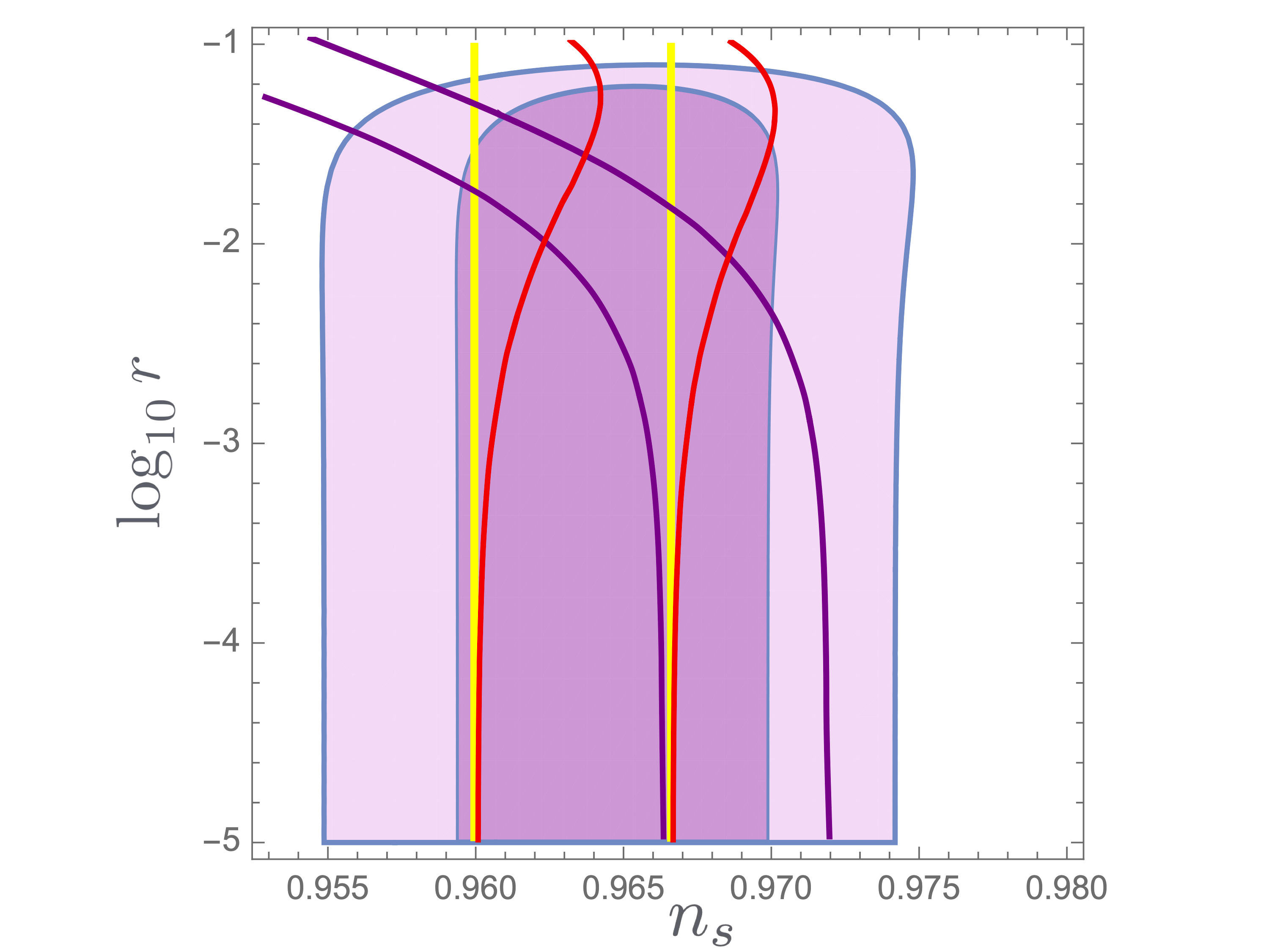
Figure 2: A combined plot of predictions of the simplest T-models (bounded by two yellow lines corresponding to $50\leq N_{e}\leq 60$) the simplest E-models (bounded by red lines) and the KKLTI model (bounded by purple lines) Kallosh:2019hzo .

During inflation the mass squared of the heavy fields $\phi_{M},a_{M}$ remain approximately the same as it was at Step I, so it can take any value up to the Planck mass. This means that the fields $\phi_{M}$ and $a_{M}$ are strongly stabilized at $\phi_{M}=a_{M}=0$. The mass squared of the imaginary component $a$ of the inflaton field field $T={1\over\sqrt{2}}(\phi+{\rm i}a)$ is positive. Thus, the inflaton trajectory $T={1\over\sqrt{2}}\phi$, $\phi_{M}=a_{M}=a=0$ is stable. Importantly, the potential masses of the light fields $\phi$ and $a$ and the inflaton potential (32) do not depend on $M$. This ensures sequestering of the inflaton potential from the high energy scale physics related to the superpotential $W^{(I)}=M(T_{1}-T_{2})^{2}$.

The development of inflation depends on our choice of potential $V(T_{i},\overline{T}_{i})$ in eq. (31). Note that one can add to this potential various terms stabilizing the inflaton trajectory without affecting the inflaton potential $V(\phi)$. For example, any term proportional to $-(T_{i}-\overline{T}_{i})^{2}$ vanishes along the inflaton trajectory, but it allows to increase the mass squared of the axion $a$. We also note that the mass of $T_{M}$ is not much affected by the inflaton dynamics in this model because the Kähler potential is independent of the inflaton $\phi$. This might not be the case in more general setups, and we will show an example in the next section.

4 Three field model

4.1 Step I

The next model describes three fields $T_{1}$, $T_{2}$ and $T_{3}$:

$$K^{(I)} = -\sum_{i=1}^{3}\ln(T_{i}+\overline{T}_{i})\,,\qquad W^{(I)}={1\over 4}(T_{1}-T_{2})(T_{2}-T_{3})\ .$$ (34)

There is a supersymmetric Minkowski flat direction $T_{1}=T_{2}=T_{3}$, corresponding to a massless field

$$T={1\over 3}(T_{1}+T_{2}+T_{3})\ .$$ (35)

There are also two heavy fields $T_{M_{1}}$, $T_{M_{2}}$, which correspond to some other combinations of the fields $T_{1},T_{2},T_{3}$.

The fields $T_{i}$ can be represented as $T_{i}=e^{-\sqrt{2}\,\phi_{i}}\,(1+{\rm i}\sqrt{2}a_{i})$, where the fields $\phi_{i}$ and the fields $a_{i}$ are canonical in the small $a_{i}$ limit. When $\phi_{i}={1\over\sqrt{3}}\phi$ and $a_{i}=0$ the mass squared eigenvalues of the canonically normalized fields $\phi_{i}$ are:

$$m^{2}=0,\qquad m^{2}=\frac{9}{8}\,e^{-\sqrt{2\over 3}\phi},\qquad m^{2}=\frac{1}{8}\,e^{-\sqrt{2\over 3}\phi}\ .$$ (36)

The masses of the heavy fields change depending on $\phi$. Therefore, we must check at Step II whether the heavy fields remain heavy during inflation and decouple from the inflationary dynamics.

4.2 Step II

The Kähler  potential and superpotential are

$$K^{(II)} = -\sum_{i=1}^{3}\ln(T_{i}+\overline{T}_{i})+{F_{X}^{2}\over F_{X}^{2}+V_{\rm infl}(T_{i},\overline{T}_{i})}X\overline{X}\ ,$$ (37)

$$W^{(II)} = W^{(I)}+(W_{0}+XF_{X})\left(\prod_{i=1}^{3}2T_{i}\right)^{1/2}.$$ (38)

Our choice of the potential in equation (38) with $T$ defined in equation (35) is

$$V_{\rm infl}(T_{i},\overline{T}_{i})=\mu^{2}\left(1-\frac{1}{3}\sum_{i=1}^{3}T_{i}\right)\left(1-\frac{1}{3}\sum_{i=1}^{3}\overline{T}_{i}\right)\quad\to\quad V_{\rm infl}(T,\overline{T})=\mu^{2}(1-T)(1-\overline{T}).$$ (39)

In the first approximation, let us follow the supersymmetric trajectory $T_{1}=T_{2}=T_{3}=T$ on which the Kähler and superpotential are reduced to

$$K=-3\ln(T+\overline{T})+{F_{X}^{2}\over F_{X}^{2}+V_{\rm infl}(T,\overline{T})}X\overline{X},\qquad W=(2T)^{\frac{3}{2}}(W_{0}+F_{X}X).$$ (40)

At $T_{1}=T_{2}=T_{3}$ and $T_{i}=\overline{T}_{i}$ the potential depends on the field $T=t=e^{-\sqrt{2\over 3}\phi}$ and is given by

$$V_{\rm total}(t)=\Lambda+\mu^{2}(1-t)^{2}=\Lambda+\mu^{2}\left(1-e^{-\sqrt{2\over 3}\phi}\right)^{2}\ .$$ (41)

Here with $\Lambda=F_{X}^{2}-3W_{0}^{2}>0$, inflation ends at $t=1,\phi=0$ in a de Sitter vacuum. This is the $\alpha=1$ attractor model, whose bosonic part coincides with that of the Starobinsky model.

In order to make sure that the sequestering mechanism works consistently, we need to check the behaviour of the two heavy fields during inflation. The masses of them calculated by using eqs. (38) are presented in Fig. 3, for the choice of parameters $W_{0}=F_{X}/\sqrt{3}=10^{-5},\ \mu=10^{-5}$. The axion masses of these heavy superfields are only slightly different from the saxion masses plotted here, this difference is due to the small values of the parameters $W_{0}=F_{X}/\sqrt{3}=10^{-5},\ \mu=10^{-5}$.

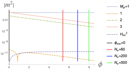
Figure 3: Here we plot, using the logarithmic scale, the absolute value of the masses squared of the heavy fields, the two top lines, not far from the $M_{Pl}=1$ scale. The absolute value of the mass squared of the inflaton field is many order of magnitudes lighter: This is the uplifted flat direction of Step I, the inflaton field. The kink at $\phi\approx 0.8$ is due to the fact that the inflaton mass squared, which was negative during early stages of inflation, and then vanishes and changes its sign, and we plot logarithm of its absolute value. The actual mass squared of the inflaton field is shown in Fig. 3.

The mass squared of the inflaton is negative at the plateau of the potential and flips sign at $\phi\approx 0.8$, at which the absolute value of the inflaton mass squared shows a singular behavior in Fig. 4.

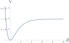
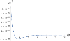
Figure 4: The left panel shows the inflaton plateau potential of the $\alpha=1$ attractor model in equation (41) for $\Lambda=0$ and $\mu=10^{-5}$. The right panel shows the inflaton mass squared.

The heavy masses of the directions orthogonal to the inflationary trajectory ensure the validity of the sequestering mechanism, and we can safely use the effective description given by eq. (41). It is also worth emphasizing that the effective Kähler potential acquires the different Kähler  curvature radius, $\alpha_{1,2,3}=\frac{1}{3}\to\alpha_{T}=1$. Thus, the sequestering not only removes the heavy degrees of freedom, but also affects the inflationary dynamics.

5 Discussion

In this paper we described and further developed a basic mechanism which allows us to obtain inflationary models sequestered from physics at the Planckian energy scale. We illustrated this mechanism through several relatively simple examples. This mechanism was used in Gunaydin:2020ric to construct inflationary models in M-theory.

At Step I, considering the case of one flat direction for simplicity, we find one massless supermultiplet and some number of heavy supermultiplets. At Step II we find that all heavy multiplets remain sufficiently heavy, with some split of masses inside the supermultiplet due to supersymmetry breaking. Meanwhile the massless multiplet of Step I is uplifted in a way which leads to a plateau potential for the real part of the superfield, i.e., for a single field inflation model. The axion field orthogonal to the inflationary trajectory is stabilized at vanishing value of the axion due to supersymmetry breaking and due to the choice of $V_{\rm infl}$ at Step II. Its mass is sufficiently heavy to decouple the axion from inflation despite these two fields being both massless at Step I.

In the follow-up investigation Kallosh:2021vcf , we will apply our methods to models where Step I is derived from IIB string theory. There are some specific features of such models. First of all, there are many scalar fields. We will study the STU model with 7 different moduli $S,\,T_{1},\,T_{2},\,T_{3},\,U_{1},\,U_{2},\,U_{3}$. Secondly, there are many constraints on the structure of the superpotentials in such models. The general structure of the superpotential $W_{\rm flux}(T^{i})$ that we are using is described in Aldazabal:2006up . It has terms depending on moduli starting from order zero up to order 5 in the fields. About 60 coefficients are arbitrary and are defined by various fluxes which are possible in 10D supergravity. These fluxes must satisfy about 100 tadpole cancellation conditions, which are basically Bianchi identities in the presence of local sources, such as D-branes and O-planes. It is not easy to find flux superpotentials which have supersymmetric Minkowski vacua and satisfy all tadpole conditions.

Fortunately, we have found such solutions in a class of superpotentials which are quadratic in the fields so that most of the tadpole cancellation conditions are satisfied trivially. We found solutions for the remaining tadpole cancellation conditions. We have found vacua with one flat direction $T\equiv S=T_{1}=T_{2}=T_{3}=U_{1}=U_{2}=U_{3}$ and with 3 flat directions $T_{(1)}\equiv U_{1}=U_{3}=T_{1}=T_{3}$, $T_{(2)}\equiv S=U_{2}$ , $T_{(3)}\equiv T_{2}$.

Then, using the methods outlined in the present paper, we uplifted these flat directions and studied inflation in these models. Just as in the models discussed in the present paper, the high energy scale parameters appearing in string theory and the heavy masses do not affect the inflationary dynamics. The main consequence of string theory inherited by the inflationary models is the hyperbolic geometry of the moduli space, which helps to develop $\alpha$-attractor inflationary models with the discrete set of possible values $3\alpha=7,6,5,4,3,2,1$.

References

- (1) R. Kallosh and A. Linde, Universality Class in Conformal Inflation, JCAP 1307 (2013) 002 [1306.5220].
- (2) S. Ferrara, R. Kallosh, A. Linde and M. Porrati, Minimal Supergravity Models of Inflation, Phys. Rev. D88 (2013) 085038 [1307.7696].
- (3) R. Kallosh, A. Linde and D. Roest, Superconformal Inflationary -Attractors, JHEP 11 (2013) 198 [1311.0472].
- (4) M. Galante, R. Kallosh, A. Linde and D. Roest, Unity of Cosmological Inflation Attractors, Phys. Rev. Lett. 114 (2015) 141302 [1412.3797].
- (5) Planck collaboration, Y. Akrami et al., Planck 2018 results. X. Constraints on inflation, Astron. Astrophys. 641 (2020) A10 [1807.06211].
- (6) R. Kallosh and A. Linde, CMB targets after the latest Planck data release, Phys. Rev. D 100 (2019) 123523 [1909.04687].
- (7) R. Kallosh, A. Linde, D. Roest and Y. Yamada, induced geometric inflation, JHEP 07 (2017) 057 [1705.09247].
- (8) E. McDonough and M. Scalisi, Inflation from Nilpotent Kähler Corrections, JCAP 1611 (2016) 028 [1609.00364].
- (9) A. Linde, Gravitational waves and large field inflation, JCAP 1702 (2017) 006 [1612.00020].
- (10) P. Binétruy and M. K. Gaillard, Candidates for the inflaton field in superstring models, Phys. Rev. D 34 (1986) 3069.
- (11) M. K. Gaillard, H. Murayama and K. A. Olive, Preserving flat directions during inflation, Phys. Lett. B 355 (1995) 71 [hep-ph/9504307].
- (12) J. Ellis, M. A. G. Garcia, N. Nagata, N. D. V., K. A. Olive and S. Verner, Building models of inflation in no-scale supergravity, Int. J. Mod. Phys. D 29 (2020) 2030011 [2009.01709].
- (13) E. Silverstein and A. Westphal, Monodromy in the CMB: Gravity Waves and String Inflation, Phys. Rev. D 78 (2008) 106003 [0803.3085].
- (14) D. Baumann and D. Green, Desensitizing Inflation from the Planck Scale, JHEP 09 (2010) 057 [1004.3801].
- (15) D. Baumann and D. Green, Inflating with Baryons, JHEP 04 (2011) 071 [1009.3032].
- (16) X. Dong, B. Horn, E. Silverstein and A. Westphal, Simple exercises to flatten your potential, Phys. Rev. D 84 (2011) 026011 [1011.4521].
- (17) L. McAllister, E. Silverstein, A. Westphal and T. Wrase, The Powers of Monodromy, JHEP 09 (2014) 123 [1405.3652].
- (18) M. Gunaydin, R. Kallosh, A. Linde and Y. Yamada, M-theory Cosmology, Octonions, Error Correcting Codes, JHEP 01 (2021) 160 [2008.01494].
- (19) J. J. M. Carrasco, R. Kallosh, A. Linde and D. Roest, Hyperbolic geometry of cosmological attractors, Phys. Rev. D92 (2015) 041301 [1504.05557].
- (20) S. Ferrara and R. Kallosh, Seven-disk manifold, -attractors, and modes, Phys. Rev. D94 (2016) 126015 [1610.04163].
- (21) R. Kallosh, A. Linde, T. Wrase and Y. Yamada, Maximal Supersymmetry and B-Mode Targets, JHEP 04 (2017) 144 [1704.04829].
- (22) R. Kallosh, A. Linde and Y. Yamada, Planck 2018 and Brane Inflation Revisited, JHEP 01 (2019) 008 [1811.01023].
- (23) J. Martin, C. Ringeval and V. Vennin, Encyclopædia Inflationaris, Phys. Dark Univ. 5-6 (2014) 75 [1303.3787].
- (24) S. Kachru, R. Kallosh, A. D. Linde and S. P. Trivedi, De Sitter vacua in string theory, Phys. Rev. D68 (2003) 046005 [hep-th/0301240].
- (25) S. Kachru, R. Kallosh, A. D. Linde, J. M. Maldacena, L. P. McAllister and S. P. Trivedi, Towards inflation in string theory, JCAP 0310 (2003) 013 [hep-th/0308055].
- (26) R. Kallosh, A. Linde, T. Wrase and Y. Yamada, IIB String Theory and Sequestered Inflation, 2108.08492.
- (27) G. Aldazabal, P. G. Camara, A. Font and L. E. Ibanez, More dual fluxes and moduli fixing, JHEP 05 (2006) 070 [hep-th/0602089].