Gravitational waves from cosmological compact binaries

Abstract

We consider gravitational waves emitted by various populations of compact binaries at cosmological distances. We use population synthesis models to characterize the properties of double neutron stars, double black holes and double white dwarf binaries as well as white dwarf-neutron star, white dwarf-black hole and black hole-neutron star systems.
We use the observationally determined cosmic star formation history to reconstruct the redshift distribution of these sources and their merging rate evolution.
The gravitational signals emitted by each source during its early-inspiral phase add randomly to produce a stochastic background in the low frequency band with spectral strain amplitude between $\sim 10^{-18}\,\mbox{Hz}^{-1/2}$ and $\sim 5\times 10^{-17}\,\mbox{Hz}^{-1/2}$ at frequencies in the interval $[\sim 5\times 10^{-6}-5\times 10^{-5}]$ Hz.

The overall signal which, at frequencies above $10^{-4}$ Hz, is largely dominated by double white dwarf systems, might be detectable with LISA in the frequency range $[1-10]$ mHz and acts like a confusion limited noise component which might limit the LISA sensitivity at frequencies above 1 mHz.

1 Introduction

Binaries with two compact stars are the most promising sources for gravitational radiation. The final phase of spiral in may be detected with ground-based (LIGO, VIRGO, GEO and TAMA) and space-borne laser interferometers (LISA). This has motivated researchers to model gravitational waveforms and to develop population synthesis codes to estimate the properties and formation rates of possible sources for gravitational wave radiation.

Since there is not yet a single prescription for calculating the gravitational emission from a compact binary system, it is customary to divide the gravitational waveforms in two main pieces: the inspiral waveform, emitted before tidal distortions become noticeable, and the coalescence waveform, emitted at higher frequencies during the epoch of distortion, tidal disruption and/or merger (Cutler et al. 1993).

As the binary, driven by gravitational radiation reaction, spirals in, the frequency of the emitted wave increases until the last 3 orbital cycles prior to complete merger.

With post-Newtonian expansions of the equations of motion for two point masses, the waveforms can be computed fairly accurately in the relatively long phase of spiral in (see, for a recent review, Rasio & Shapiro 2000 and references therein). Conversely, the gravitational waveform from the coalescence can only be obtained from extensive numerical calculations with a fully general relativistic treatment. Such calculations are now well underway (Brady, Creighton & Thorne 1998; Damour, Iyer & Sathyaprakash 1998; Rasio & Shapiro 1999).

In this paper, we consider the low frequency signal from the early phase of the spiral in, which is of interest for space-borne antennas, such as LISA. For this purpose, we use the leading order expression for the single source emission spectrum, obtained using the quadrupole approximation. Our analysis includes various populations of compact binary systems: black hole-black hole (bh, bh), neutron star-neutron star (ns, ns), white dwarf-white dwarf (wd, wd) as well as mixed systems such as (ns, wd), (bh, wd) and (bh, ns).

For some of these sources [(ns, ns), (wd, wd) and (ns, wd)], statistical information on the event rate can be inferred from electromagnetic observations. In particular, there are several observational estimates of the (ns, ns) merger rate obtained from statistics of the known population of binary radio pulsars (Narayan, Piran & Shemi 1991; Phinney 1991).

A rather large number of close white dwarf binaries have recently been found (see Maxted & Marsh 1999 and Moran 1999). However, it is customary to constrain the (wd, wd) merger rate from the observed SNIa rate (see Postnov & Prokhorov 1998). Also the population of binaries where a radio pulsar is accompanied by a massive unseen white dwarf may be considerably higher than hitherto expected (Portegies Zwart & Yungelson 1999).

Since most stars are members of binaries and the formation rate of potential sources of gravitational waves may be abundant in the Galaxy, the gravitational-wave signal emitted by such binaries might produce a stochastic background. This possibility has been explored by various authors, starting from the earliest work of Mironovskij (1965) and Rosi & Zimmermann (1976) until the more recent investigations of Hils, Bender & Webbink (1990), Lipunov et al. (1995), Bender & Hils (1997), Giazotto, Bonazzola & Gourgoulhon (1997), Giampieri (1997), Postnov & Prokhorov (1998), and Nelemans, Portegies Zwart & Verbunt (1999). This background, which acts like a noise component for the interferometric detectors, has always been viewed as a potential obstacle for the detection of gravitational wave backgrounds coming from the early Universe.

In this paper we extend the investigation of compact binary systems to extragalactic distances, accounting for the binaries which have been formed since the onset of galaxy formation in the Universe. Following Ferrari, Matarrese & Schneider (1999a, 1999b: hereafter referred as FMSI and FMSII, respectively), we modulate the binary formation rate in the Universe with the cosmic star formation history derived from observations of field galaxies out to redshift $z\sim 5$ (see e.g. Madau, Pozzetti & Dickinson 1998b; Steidel et al. 1999).

The magnitude and frequency distribution of the integrated gravitational signal produced by the cosmological population of compact binaries is calculated from the distribution of binary parameters (masses and types of both stars, orbital separations and eccentricities). These orbital parameters characterize the gravitational-wave signal which we observe on Earth.

Detailed information for the properties of the binary population may be obtained through population synthesis. We use the binary population synthesis code SeBa to simulate the characteristics of the binary population in the Galaxy (Portegies Zwart & Verbunt 1996; Portegies Zwart & Yungelson 1998). The characteristics of the extragalactic population are derived from extrapolating these results to the local Universe.

The paper is organized as follows: in Section 2 we describe the population synthesis calculations. Section 3 deals with the energy spectrum of a single source followed, in Section 4, by the derivation of the extragalactic backgrounds for the different binary populations. In Sections 3 and 4 we also give details on the adopted astrophysical and cosmological properties of the systems. In Section 5, we compute the spectral strain amplitude produced by each cosmological population and investigate its detectability with LISA. Finally, in Section 6 we summarize our main results and compare them with other previously estimated astrophysical background signals.

2 Population synthesis model

In order to characterize the main properties of different compact binary systems, we use the binary population synthesis program SeBa of Portegies Zwart & Yungelson (1998). Details of the code can be found in (Portegies Zwart & Yungelson 1998). Here, we simply recall the main assumptions of their adopted model B, which satisfactorily reproduces the properties of observed high-mass binary pulsars (with neutron star companions).

The following initial conditions were assumed: the mass of the primary star $m_{1}$ is determined using the mass function described by Scalo (1986) between 0.1 and 100 $M_{\odot}$. For a given $m_{1}$, the mass of the secondary star $m_{2}$ is randomly selected from a uniform distribution between a minimum of 0.1 $M_{\odot}$ and the mass of the primary star. The semi-major axis distribution is taken flat in $\log a$ (Kraicheva et al. 1978) ranging from Roche-lobe contact up to $10^{6}$ R_⊙ (Abt & Levy 1978; Duquennoy & Mayor 1991). The initial eccentricity distribution is independent of the other orbital parameters, and is $\Xi(e)=2e$.

Neutron stars receive a velocity kick upon birth. Following Hartman et al. (1997), model B assumes the distribution for isotropic kick velocities (Paczyński 1990),

$$P(u)du={4\over\pi}\cdot{du\over(1+u^{2})^{2}},$$ (1)

with $u=v/\sigma$ and $\sigma=600\,\,\mbox{km}\,\mbox{s}^{-1}$.

The birthrate of the various compact binaries is normalized to the Type II+Ib/c supernova rate (see Portegies Zwart & Verbunt 1996). The supernova rate of 0.01 per year was assumed to be constant over the lifetime of the galactic disc ($\sim 10$ Gyr).

When computing the birth and merger-rates we account for the time-delay between the formation of the progenitor system and that of the corresponding degenerate binary, $\tau_{s}$. Its value is set by the time it takes for the least massive between the two companion stars to evolve on the main sequence. For (bh, bh), (ns, ns) and (bh, ns) systems $\tau_{s}\lower 2.15277pt\hbox{$\;\buildrel<\over{\sim}\;$}50$ Myr and it is negligible compared to the assumed lifetime of the galactic disc. Conversely, (wd, wd), (ns, wd) and (bh, wd) binaries follow a slower evolutionary clock and $\tau_{s}$ can be considerably larger. The cumulative probability distribution, $P(<\tau_{s})$, predicted by the population synthesis code is shown in Fig. 1. For these systems $\tau_{s}$ can be as large as 10 Gyr although all systems are predicted to have $\tau_{s}\leq 10$ Gyr.

Figure 1: The cumulative probability distribution for the time delay $\tau_{s}$ (in Myr) between the formation of the progenitor system and the formation of the corresponding degenerate binary obtained for the (bh, wd), (ns, wd) and (wd, wd) samples.

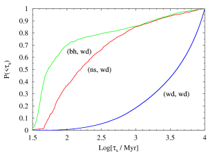
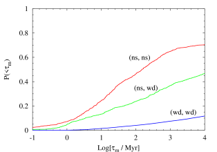
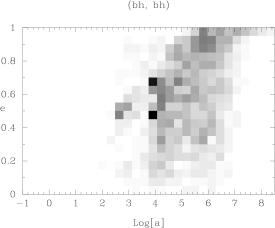
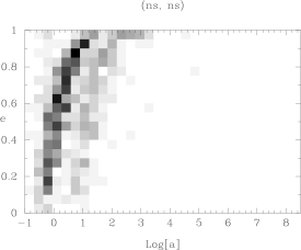
After the degenerate binary has formed, its further evolution is determined by the time it takes to radiate away its orbital energy in gravitational waves. The time between the formation of the degenerate system and its final coalescence, $\tau_{m}$, depends on the orbital configuration and on the mass of the two companion stars. The predicted cumulative probability distribution is shown in Fig. 2 for the (wd, wd), (ns, ns) and (ns, wd) samples. We see from the figure that there is a significant fraction of systems which does not merge in 10 Gyr. For (bh, bh) binaries and mixed systems with one black hole companion the population synthesis code predicts very long merger times. In particular, all (bh, bh) systems appear to have $\tau_{m}$ greater than 15 Gyr. The reason for these large merger times is that binaries with a black hole companion are characterized by very large initial orbital separations (see e.g. Fig. 3). In fact, bh progenitors are very massive stars and have a very strong stellar wind. For this reason they do not easily reach Roche-lobe over-flow and rarely experience a phase of mass transfer, which is required to reduce the orbital separation of the stars. Unfortunately, the evolution (especially the amount of mass loss in the stellar winds) of high mass stars is rather uncertain (Langer et al. 1994). The result that we obtain at least indicates that it will be very rare to observe any of these bh mergers. Recently Portegies Zwart & McMillan (1999) however identified a new channel for producing black hole binaries which are eligible to mergers on a relatively short time scale.

Figure 2: The cumulative probability distribution for the merger time $\tau_{m}$ (in Myr) is shown for the (ns, ns), (ns, wd) and (wd, wd) samples.

Figure 3: The probability distribution for the orbital parameters of (bh, bh) systems (left panel) is compared to that obtained for the (ns, ns) (right panel) population.

In Table 1, we summarize the results for all binary types that we have investigated.

Table 1: The galactic birthrates, $R_{X,gal}$, and merger rates, $R^{mrg}_{X,gal}$, obtained for each compact binary type $X$ using model B of (Portegies Zwart & Yungelson 1998), see text. The rates are normalized to the core-collapse supernova rate of $0.01\,\,\mbox{yr}^{-1}$ and 100% binarity. Merger rates are computed after 10 Gyr of the evolution of the Galaxy with a constant supernova rate.

Binary Type $X$	$R_{X,gal}\mbox{yr}^{-1}$	$R^{mrg}_{X,gal}\mbox{yr}^{-1}$
(bh, bh)	$6.3\times 10^{-5}$	NA
(bh, ns)	$1.0\times 10^{-5}$	$1.0\times 10^{-6}$
(bh, wd)	$4.4\times 10^{-5}$	$10^{-7}$
(ns, ns)	$3.6\times 10^{-5}$	$2.5\times 10^{-5}$
(ns, wd)	$3.6\times 10^{-4}$	$1.6\times 10^{-4}$
(wd, wd)	$4.4\times 10^{-2}$	$4.8\times 10^{-3}$

3 Inspiral energy spectrum of single sources

Assuming that the orbit of the binary system has already been circularized by gravitational radiation reaction, the inspiral spectrum $dE/d{\nu}$ emitted by a single source can be obtained using the quadrupole approximation (Misner, Thorne & Wheeler 1995). The resulting expression, in geometrical units (G=c=1), can be written as,

$$\frac{dE}{d\nu}=\frac{\pi}{3}\,\frac{{\cal M}^{5/3}}{(\pi\nu)^{1/3}}$$ (2)

where ${\cal M}=\mu^{3/5}M^{2/5}$ is the so-called chirp mass, $M=m_{1}+m_{2}$ stands for the total mass and $\mu=m_{1}\,m_{2}/M$ is the reduced mass.

The frequency $\nu$ at which gravitational waves are emitted is twice the orbital frequency and depends on the time left to the merger event through,

$$(\pi\nu)^{-8/3}=(\pi\nu_{max})^{-8/3}+\frac{256}{5}\,{\cal M}^{5/3}\,(t_{c}-t)$$ (3)

where $t_{c}$ is the time of the final coalescence and we terminate the inspiral spectrum at a frequency $\nu_{max}$. When Post-Newtonian expansion terms are included, it is customary to consider the inspiral spectrum as a good approximation all the way up to $\nu_{LSCO}$, i.e. the frequency of the quadrupole waves emitted at the last stable circular orbit (LSCO) (see e.g. Flanagan & Hughes 1998). However, for the purposes of our study, we neglect post-Newtonian terms and we set the value of $\nu_{max}$ to correspond to the quadrupole frequency emitted when the orbital separation is roughly 3 times the separation at the LSCO.

The value of the orbital separation at the LSCO depends on the mass ratio of the two stellar components and varies between $5M-6M$. The lower limit is obtained in the test particle approximation ($m_{1}\gg m_{2}$), whereas the upper value corresponds to the equal-mass case ($m_{1}\sim m_{2}$) (see Kidder, Will & Wiseman 1993). If we consider the equal-mass limit, which is more conservative for constraining the maximum frequency, $\nu_{LSCO}\sim 0.022/M$ and $\nu_{max}\sim 0.19\,\,\nu_{LSCO}$.

For (wd, wd) binaries and binaries with one wd companion, the maximum frequency, i.e. the minimum distance between the two stellar components, is set in order to cut-off the Roche-lobe contact stage. In fact, the mass transfer from one component to its companion transforms the original detached binary into a semi-detached binary. This process can be accompanied by the loss of angular momentum with mass loss from the system and the above description cannot be applied. Thus, for closed white dwarf binaries we require that the mimimum orbital separation is given by $r_{wd}(m_{1})+r_{wd}(m_{2})$ where

$$r_{wd}(m)=0.012R_{\odot}\sqrt{\left(\frac{m}{1.44M_{\odot}}\right)^{-2/3}-\,\,\left(\frac{m}{1.44M_{\odot}}\right)^{2/3}}$$ (4)

is the approximate formula for the radius of a white dwarf from Nauenberg (1972) (see also Portegies Zwart & Verbunt 1996).

Consider now sources at cosmological distances. The locally measured average energy flux emitted by a source at redshift $z$ is,

$$f(\nu)=\int\frac{d\Omega}{4\pi}\,\frac{dE}{d\Sigma d\nu}(\nu)=\frac{(1+z)^{2}}{4\pi d_{L}(z)^{2}}\,\,\frac{c^{3}}{G}\,\,\frac{dE_{e}}{d\nu_{e}}[\nu(1+z)]$$ (5)

where $d_{L}(z)$ is the luminosity distance to the source, $\nu=\nu_{e}\,(1+z)^{-1}$ is the observed frequency and the factor $c^{3}/G$ is needed in order to change from geometrical to physical units. Thus, the emission spectrum can be written as,

$$\frac{dE_{e}}{d\nu_{e}}[\nu(1+z)]=\frac{\pi}{3}\frac{{\cal M}^{5/3}}{[\pi\,\nu(1+z)]^{1/3}}$$ (6)

where $\nu$ is the observed frequency emitted by a system at time $t(z)$

$$(\pi\nu)^{-8/3}=(\pi\nu_{max})^{-8/3}(1+z)^{8/3}+\frac{256}{5}\,{\cal M}^{5/3}\,$$ (7)

$$\left[t(z_{f})+\tau_{m}-t(z)\right](1+z)^{8/3}$$

and we have written the time of the final coalescence $t_{c}=t(z_{c})$ in terms of the time of formation $t(z_{f})$ and of the merger-time $\tau_{m}=t(z_{c})-t(z_{f})$.

4 Extragalactic backgrounds from different binary populations

Our main purpose is to estimate the stochastic background signal generated by different populations of compact binary systems at extragalactic distances.

These gravitational sources have been forming since the onset of galaxy formation in the Universe and for each binary type $X$ [(ns, ns); (wd, wd); (bh, bh); (ns, wd); (bh, wd); (bh, ns)] we should think of a large ensemble of unresolved and uncorrelated elements, each characterized by its masses $m_{1}$ and $m_{2}$ (or $M$ and $\mu$), by its redshift and by its time-delays $\tau_{s}$ and $\tau_{m}$ [see eqns (6) and (7)].

Thus, in order to consider all contributions from different elements of the ensemble $X$, we must integrate the single source emission spectrum over the distribution functions for the masses $M$ and $\mu$, for the time-delays and for the redshifts.

The distribution functions for $\tau_{s}$ and $\tau_{m}$ depend on the binary type $X$ and have been derived from the population synthesis code discussed in the previous section. The distribution function for ${\cal M}$ can be similarly estimated.

However, $\tau_{s}$, $\tau_{m}$ and ${\cal M}$ are not independent random variables. In particular, $\tau_{m}$ and ${\cal M}$ are correlated because ${\cal M}$ defines the rate of orbital decay, once the degenerate system has formed. Thus, for each binary population $X$, we consider the joint probability distribution for $\tau_{s}$, $\tau_{m}$ and ${\cal M}$,

$$p_{X}(\tau_{s},\tau_{m},{\cal M})\,\,d\tau_{m}\,\,d\tau_{s}\,\,d{\cal M}.$$ (8)

Conversely, the redshift distribution function, i.e. the evolution of the formation rate for each binary type $X$, can be deduced from the observed cosmic star formation history out to $z\sim 5$.

In the following subsections, we illustrate the procedure we have followed to derive the birth and merger-rates for all binary populations and to compute the spectra of the corresponding stochastic gravitational backgrounds.

4.1 Cosmic star formation rate

In the last few years, the extraordinary advances attained in observational cosmology have led to the possibility of identifying actively star forming galaxies at increasing cosmological look-back times (see, for a thorough review, Ellis 1997). Using the rest-frame UV-optical luminosity as an indicator of the star formation activity and integrating on the overall galaxy population, the data obtained with the Hubble Space Telscope (HST Madau et al. 1996, Connolly et al. 1997, Madau et al. 1998a) Keck and other large telescopes (Steidel et al. 1996, 1999) together with the completion of several large redshift surveys (Lilly et al. 1996, Gallego et al. 1995, Treyer et al. 1998) have enabled, for the first time, to derive coherent models for the star formation rate evolution throughout the Universe.
A collection of some data obtained at different redshifts is shown in the left panel of Figure 4 for a flat cosmological background model with $\Omega_{\Lambda}=0$, $h=0.5$ and a Scalo (1986) IMF with masses in the range $0.1-100M_{\odot}$.

Figure 4: The Log of the star formation rate density in units of $M_{\odot}\mbox{yr}^{-1}\mbox{Mpc}^{-3}$ as a function of redshift for a cosmological background model with $\Omega_{M}=1$, $\Omega_{\Lambda}=0$, $H_{0}=50\,\mbox{km}\mbox{s}^{-1}\mbox{Mpc}^{-1}$ and a Scalo (1986) IMF. Left: The data points correspond to UV, H$\alpha$ and IR observations of field galaxies. (Filled dots) UV observations of Treyer et al. (1998), Lilly et al. (1996), Connolly et al. (1997), HDF Madau et al. (1996), Steidel et al. (1996),(1999); (asterisks) H$\alpha$ observations of Gallego et al. 1995, Gronwall 1999, Tresse & Maddox 1998, Glazebrook et al. 1998, Yan et al. 1999); (triangles): ISO IR observations (Flores et al. 1999) and the lower limit of SCUBA data (Hughes et al. 1998). (Right): The dust-corrected SFR density as derived from UV data in the two models most favoured by observations predicted by Calzetti & Heckman (asterisks) and by Pei, Fall & Hauser filled dots (see text).

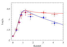
Although the strong luminosity evolution observed between redshift 0 and 1-2 is believed to be quite firmly established, the behaviour of the star formation rate at high redshift is still relatively uncertain. In particular, the decline of the star formation rate density implied by the $<z>\,\sim 4$ point of the Hubble Deep Field (HDF, see Fig. 4) is now contradicted by the star formation rate density derived from a new ground-based sample of Lyman break galaxies with $\langle z\rangle\,=4.13$ (Steidel et al. 1999) which, instead, seems to indicate that the star formation rate density remains substantially constant at $z>1-2$. It has been suggested that this discrepancy might be caused by problems of sample variance in the HDF point at $<z>\,=4$ (Steidel et al. 1999).

Because dust extinction can lead to an underestimate of the real UV-optical emission and, ultimately, of the real star formation activity, the data shown in the left panel of Fig. 4 need to be corrected upwards according to specific models for the evolution of dust opacity with redshift. In the right panel of Fig. 4, the data have been dust-corrected according to factors obtained by Calzetti & Heckman (1999) and by Pei, Fall & Hauser (1999). Using different approaches, these authors have recently investigated the cosmic histories of stars, gas, heavy elements and dust in galaxies using as inputs the available data from quasar absorption-line surveys, optical and UV imaging of field galaxies, redshift surveys and the COBE DIRBE and FIRAS measurements of the cosmic IR background radiation. The solutions they obtain appear to reproduce remarkably well a variety of observations that were not used as inputs, among which the SFR at various redshifts from H$\alpha$, mid-IR and submm observations and the mean abundance of heavy elements at various epochs from surveys of damped Lyman-$\alpha$ systems.

As we can see from the right panel of Fig. 4, spectroscopic and photometric surveys in different wavebands point to a consistent picture of the low-to-intermediate redshift evolution: the SFR density rises rapidly as we go from the local value to a redshift between $\sim 1-2$ and remains roughly flat between redshifts $\sim 2-3$. At higher redshifts, two different evolutionary tracks seem to be consistent with the data: the SFR density might remain substantially constant at $z\lower 2.15277pt\hbox{$\;\buildrel>\over{\sim}\;$}2$ (Calzetti & Heckman 1999) or it might decrease again out to a redshift of $\sim 4$ (Pei, Fall & Hauser 1999). Hereafter, we always indicate the former model as ’monolithic scenario’ and the latter as ’hierarchical scenario’ although this choice is only ment to be illustrative. In fact, preliminary considerations have pointed out that a constant SFR activity at high redshifts might not be unexpected in hiererachical structure formation models (Steidel et al. 1999).

Thus, we have updated the star formation rate model that we have considered in previous analyses (FMSI, FMSII), even though the gravitational wave backgrounds are more contributed by low-to-intermediate redshift sources than by distant ones. In addition, if a larger dust correction factor should be applied at intermediate redshifts, this would result in a similar amplification of the gravitational background spectra.

4.2 Birth and merger rate evolution

Following the method we have previously proposed (FMSI, FMSII), for each binary type $X$ the birth and merger-rate evolution could be computed from the observed star formation rate evolution. However, this procedure proves to be unsatisfactory because it fails to provide a fully consistent normalization. Its main weakness is that, even if we assume 100% of binarity, i.e. that all stars are in binary systems, the star formation histories that we have described above are not corrected for the presence of secondary stars. For the mass distributions that we have considered, secondary stars are expected to give a significant contribution to the observed UV luminosity as they account for $\sim 1/3$ of the fraction of mass in stars more massive than $8\,M_{\odot}$.

In order to circumvent the necessity of extrapolating the UV luminosity indication of massive star formation to the full range of stellar masses predicted by the model, we could directly normalize to the rate of core-collapse supernovae. This is consistent with the adopted normalization for galactic rates.

The core-collapse supernova rate can be directly derived from the observed UV luminosity at each redshift, as stars which dominate the UV emission from a galaxy are the same stars which, at the end of the nuclear burning, explode as Type II+Ib/c SNae. Moreover, the supernova rate is observed independently of the SFR. Therefore it can be used as an alternative normalization.

Figure 5: The rest-frame frequency of core-collapse SNae vs redshift predicted by the monolithic and hierarchical models. The predictions are consistent with the observed value for the present-day galaxy population (see text).

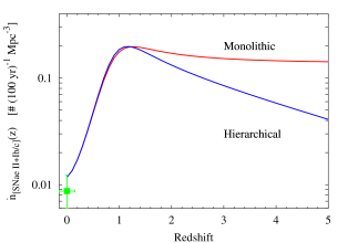
The rates of core-collapse supernovae predicted by the models shown in Fig. 4 are shown in Fig. 5 assuming a flat cosmological background model with zero cosmological constant and $h=0.5$.

In the same figure, we have plotted the available observations for the core-collapse supernova frequency in the local Universe (Cappellaro et al. 1997, Tamman et al. 1994, Evans et al. 1989, see also Madau et al. 1998b).

The binary birthrate per entry per year and comoving volume $\dot{\eta}(z)$ can be related to the core-collapse supernova rate $\dot{n}_{[SNaeII+Ib/c]}(z)$ shown in Fig. 5 in the following way,

$$\dot{\eta}(z)=\frac{\dot{n}_{[SNaeII+Ib/c]}(z)}{N_{[SNaeII+Ib/c]}}$$ (9)

where $N_{[SNaeII+Ib/c]}$ is the total number of core-collapse supernovae that we find in the simulation.

In order to estimate, from $\dot{\eta}(z)$, the birth and merger-rate evolution of a degenerate binary population $X$, we need to multiply eq. (9) by the number of type $X$ systems in the simulated samples, $N_{X}$, and we also need to properly account for both $\tau_{s}$ and $\tau_{m}$.

We shall assume that the redshift at the onset of galaxy formation in the Universe is $z_{F}=5$ and that a zero-age main sequence binary forms at a redshift $z_{s}$. After a time interval $\tau_{s}$, the system has evolved into a degenerate binary. Then, the redshift of formation of the degenerate binary system, $z_{f}$, is defined as $t(z_{f})=t(z_{s})+\tau_{s}$. The system then evolves according to gravitational wave reaction until, after a time interval $\tau_{m}$, it finally merges. Thus, the redshift at which coalescence occurs, $z_{c}$, is given by $t(z_{c})=t(z_{f})+\tau_{m}$.

This simple picture implies that the number of $X$ systems formed per unit time and comoving volume at redshift $z_{f}$ is

$$\dot{n}_{X}(z_{f}) = \int\!\!d\tau_{m}\,d{\cal M}\int_{0}^{t(z_{f})-t(z_{F})}\!\!d\tau_{s}\,\,f_{X}$$

$$\frac{\dot{n}_{[SNaeII+Ib/c]}(z_{s})}{(1+z_{s})}\,p_{X}(\tau_{s},\tau_{m},{\cal M})$$

where $f_{X}=N_{X}/N_{[SNaeII+Ib/c]}$ and $z_{s}$ is defined by $t(z_{s})=t(z_{f})-\tau_{s}$.

If we write,

$$p_{X}(\tau_{s},\tau_{m},{\cal M})=\frac{1}{N_{X}}\sum_{i}^{N_{X}}\,\delta(\tau_{s}-\tau_{s,i})\,\delta(\tau_{m}-\tau_{m,i})\,\delta({\cal M}-{\cal M}_{i})$$ (11)

where $\tau_{s,i}$, $\tau_{m,i}$ and ${\cal M}_{i}$ indicate the time delays and the chirp mass for the $i^{th}$ element of the ensemble $X$, the birthrate reads,

$$\dot{n}_{X}(z_{f}) = \frac{1}{N_{[SNaeII+Ib/c]}}\,\,\sum_{i}^{N_{X}}\,\frac{\dot{n}_{[SNaeII+Ib/c]}(z_{s})}{(1+z_{s})}$$

$$\Theta[t(z_{f})-t(z_{F})-\tau_{s,i}]$$

where $\Theta(x)$ is the step-function.

Similarly, the number of $X$ systems per unit time and comoving volume which merge at redshift $z_{c}$ is,

$$\dot{n}^{mrg}_{X}(z_{c})=\int_{0}^{t(z_{c})-t(z_{F})}\!\!d\tau_{m}\int_{0}^{t(z_{c})-\tau_{m}-t(z_{F})}\!\!d\tau_{s}\,\,\,f_{X}$$ (13)

$$\frac{\dot{n}_{[SNaeII+Ib/c]}(z_{s})}{(1+z_{s})}\int d{\cal M}\,\,p_{X}(\tau_{s},\tau_{m},{\cal M})$$

where $z_{s}$ is defined by $t(z_{s})=t(z_{c})-\tau_{m}-\tau_{s}$. If we apply eq. (11), we can write the merger-rate in a form similar to eq. (4.2), i.e.

$$\dot{n}^{mrg}_{X}(z_{c}) = \frac{1}{N_{[SNaeII+Ib/c]}}\,\,\sum_{i}^{N_{X}}\,\frac{\dot{n}_{[SNaeII+Ib/c]}(z_{s})}{(1+z_{s})}$$

$$\Theta[t(z_{c})-t(z_{F})-\tau_{s,i}-\tau_{m,i}].$$

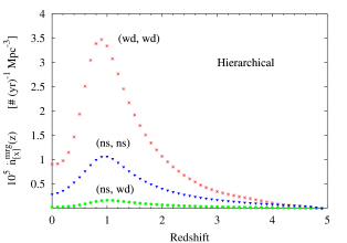
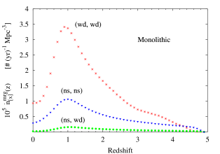
Using this procedure, we compute the birth and merger-rates for all the synthetic binary populations. The results are presented in Figs. 6, 7 and 8.

Due to their relatively small $\tau_{s}$ compared to the cosmic time, the birthrates of (bh, bh), (ns, ns) and (bh, ns) systems closely trace the UV-luminosity evolution, although with different amplitudes. Our simulation suggests that (bh, bh) systems are more numerous than (ns, ns) or (bh, ns) (see Fig. 6).

Figure 6: The formation rate of (bh, bh) (asterisks), (ns, ns) (dots) and (bh, ns) (triangles) binaries as a function of $z$ is shown for hierarchical (upper panel) and monolithic (lower panel) scenarios for a flat cosmological background.

Conversely, Fig. 7 shows that the birthrates of (wd, wd), (ns, wd) and (bh, wd) systems misrepresent the original UV-luminosity evolution as a consequence of their large $\tau_{s}$. The largest is the characteristic time-delay $\tau_{s}$, the more the maximum is shifted versus lower redshifts because the intense star formation activity observed at $z\lower 2.15277pt\hbox{$\;\buildrel>\over{\sim}\;$}2$, especially for monolithic scenarios, boosts the formation of degenerate systems at $z\lower 2.15277pt\hbox{$\;\buildrel<\over{\sim}\;$}2$. For hierarchical scenarios, if the redshift at which significant star formation begins to occur is $z_{F}\sim 5$, the birthrate of degenerate systems at redshifts $\lower 2.15277pt\hbox{$\;\buildrel>\over{\sim}\;$}4$ is almost negligible.

Figure 7: The formation rate of (wd, wd) (asterisks), (ns, wd) (dots) and (bh, wd) (triangles) binaries as a function of $z$ is shown for hierarchical (upper panel) and monolithic (lower panel) scenarios for a flat cosmological background.

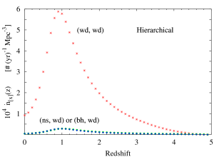
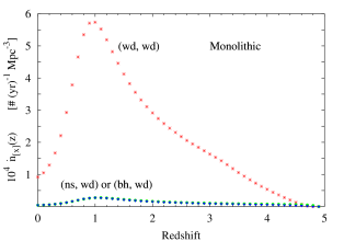
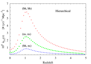
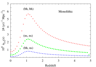
Finally, in Fig. 8, we have shown the predicted merger-rate for (wd, wd), (ns, ns) and (ns, wd) systems. In this case, the distortion of the original UV-luminosity evolution is even more apparent, particularly for monolithic scenarios. The redshift at which the maximum merger-rate occurs as well as the high redshift tail reflects the different $\tau_{m}$ distributions of these populations. We have not shown the merger-rates for (bh, bh), (bh, wd) and (bh, ns) binaries because, as we have discussed in the previous section, these systems are predicted to have merger-rates consistent with zero throughout the history of the Universe as a consequence of their very large initial orbital separations.

Figure 8: The merger-rate of (wd, wd) (asterisks), (ns, ns) (dots) and (ns, wd) (triangles) binaries as a function of $z$ is shown for hierarchical (upper panel) and monolithic (lower panel) scenarios for a flat cosmological background.

4.3 Stochastic backgrounds

Having characterized each ensemble $X$ by the distribution of chirp mass and time delays, $p_{X}(\tau_{s},\tau_{m},{\cal M})$, and by the birthrate density evolution per entry $\dot{\eta}(z)$, we can sum up the gravitational signals coming from all the elements of the ensemble. The spectrum of the resulting stochastic background, for a binary type $X$ and at a given observation frequency $\nu$, is given by the following expression,

$$\frac{dE}{d\Sigma dtd\nu}[\nu] = \int_{0}^{z_{F}}\!\!dz_{f}\int_{0}^{t(z_{f})-t(z_{F})}\!\!\!d\tau_{s}\frac{N_{X}\,\dot{\eta}(z_{s})}{(1+z_{s})}$$

$$\int_{0}^{\infty}\!\!d{\cal M}\,d\tau_{m}\,p_{X}(\tau_{s},\tau_{m},{\cal M})\,\frac{dV}{dz_{e}^{*}}\,f[\nu,z_{e}^{*}]$$

where $z_{F}$ is the redshift of the onset of star formation in the Universe, $z_{f}$ is the redshift of formation of the degenerate binary systems, $z_{s}$ is the redshift of formation of the corresponding progenitor system defined by $t(z_{s})=t(z_{f})-\tau_{s}$, $f[\nu,z_{e}^{*}]$ is given by eq. (5) and $z_{e}^{*}$ is the redshift of emission that an element of the ensemble must have in order to contribute to the energy density at the observation frequency $\nu$.

It follows from eq. (7) that, for a given observation frequency $\nu$, $z_{e}^{*}$ is a function of $z_{f}$, $\tau_{m}$, ${\cal M}$ and $\nu_{max}$. In principle, an inspiraling compact binary system emits a continuous signal from its formation to its final coalescence thus, $z_{c}\leq z_{e}\leq z_{f}$. However, in eq. (4.3) we do not restrict to systems which reach their final coalescence at $z_{c}\geq 0$ as we are interested to any source between $z=0$ and $z=z_{F}$ emitting gravitational waves during its early inspiral phase. Therefore, the signals which contribute to the local energy density at observation frequency $\nu$ might be emitted anywhere between $\mbox{sup}[0,z_{c}]\leq z_{e}^{*}\leq z_{f}$, provided that,

$$(\pi\nu)^{-8/3}=(\pi\nu_{max})^{-8/3}(1+z_{e}^{*})^{8/3}+\frac{256}{5}\,{\cal M}^{5/3}$$ (16)

$$\left[t(z_{f})+\tau_{m}-t(z_{e}^{*})\right](1+z_{e}^{*})^{8/3}.$$

Substituting eq. (11) in eq. (4.3), we can write the background energy density generated by a population $X$ in the form,

$$\frac{dE}{d\Sigma dtd\nu}[\nu] = \int_{0}^{z_{F}}\!\!dz_{f}\sum_{i}^{N_{X}}\frac{\dot{\eta}(z_{s})}{(1+z_{s})}$$

$$\Theta[t(z_{f})-t(z_{F})-\tau_{s,i}]\,\frac{dV}{dz_{e}^{*}}\,f[\nu,z_{e}^{*}]$$

where $z_{e}^{*}$ satisfies eq. (16).

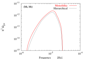
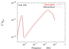
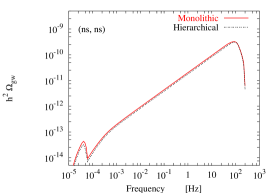
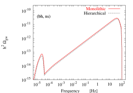
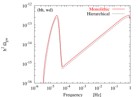
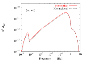
The predicted spectral energy densities for the populations of degenerate binary types that we have considered are plotted in Fig. 9. For each binary type, we show the results obtained assuming both monolithic and hierarchical scenarios for the evolution of the underlying galaxy population.

Figure 9: The spectral energy density of the gravitational background produced by various extragalactic populations of degenerate binaries in monolithic and hierarchical scenarios assuming a flat cosmological background with zero cosmological constant.

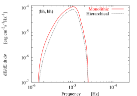
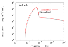
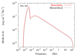
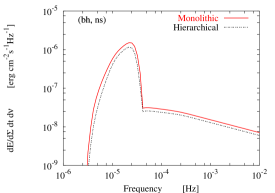
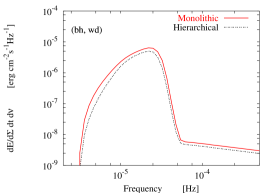
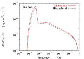
The spectral energy densities are characterized by the presence of a sharp maximum which, depending on the binary population, has an amplitude spanning about two orders of magnitudes, in the frequency range $[10^{-5}-10^{-4}]$ Hz. In the following, we refer to this part of the signal as ’primary’ component. At higher frequencies, a ’secondary’ component appears for all but (bh, bh) systems. The frequency which marks the transition between primary and secondary components as well as their relative amplitudes depend sensitively on the population.

The reason why (bh, bh) systems do not show a secondary component is that this is entirely contributed by sources which merge before $z=0$. Conversely, the low-frequency part of the spectrum is dominated by systems with merger-times larger than a Hubble time. These sources are observed at very low frequencies because the value of the minimum frequency (which is emitted at formation, $z_{f}$) is set by the amplitude of the merger-time [see eq. (16)]. The larger is the merger-time, the smaller the minimum frequency at which the in-spiral waves are emitted. Moreover, eq. (6) shows that the flux emitted by each source decreases with frequency. This explains the larger amplitude of primary components with respect to secondary ones. For systems with merger-times larger than a Hubble time, the largest frequency is emitted at $z=0$ by binaries which form at $z_{f}\sim z_{F}$. No contribution from such objects can be observed above this critical frequency and the primary component falls rapidly to zero.

The amplitude of secondary components reflects the number of systems with moderate merger-times. The maximum frequency which might be observed is emitted by systems which are very close to their coalescence at $z=0$. Since $\nu_{max}$ is larger for (ns, ns) than for (wd, wd), the secondary component produced by double neutron stars extends up to $\sim 10^{2}$ Hz.

It is interesting to note is that monolithic scenarios predict a maximum amplitude which is a factor $\sim$ 20-25% larger than the hierarchical case. This difference is much larger than what has been previously obtained for other extragalactic backgrounds (see e.g. FMSI), indicating that the energy density produced by extragalactic compact binaries is substantially contributed by sources which form at redshifts $\lower 2.15277pt\hbox{$\;\buildrel>\over{\sim}\;$}1-2$. It is quite difficult to unveil the origin of this effect because of the large number of parameters which determine the appearance of the final energy density. However, a plausible explanation might be that, depending on its specific time-delays $\tau_{s}$ and $\tau_{m}$, each system emits the signal at redshifts which can be substantially smaller than the formation redshift of the corresponding progenitor system. Thus, although the background signal is mostly emitted at low-to-intermediate redshifts, the sources which produce these signals might have been formed at higher redshifts and reflect the state of the Universe at earlier times, when the differences among hierarchical and monolithic scenarios are more significant. Comparing the different panels of Fig. 9, we conclude that the background produced by (bh, bh) binaries has the largest amplitude but it is concentrated at frequencies below $\sim 2\times 10^{-5}$ Hz. At higher frequencies, which are more interesting from the point of view of detectability, the dominant contribution comes from (wd, wd) systems. This is consistent with what has already been found for the galactic populations (Hils, Bender & Webbink 1990).

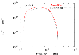
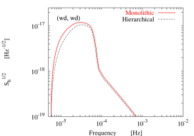
¿From the background spectrum it is possible to compute the closure density $\Omega_{gw}\,h^{2}$ and the spectral strain amplitude of the signal $S_{h}$,

$$S_{h}(\nu) = \frac{2G}{\pi c^{3}}\,\,\frac{1}{\nu^{2}}\,\,\frac{dE}{dSdtd{\nu}}({\nu}),$$ (18)

$$\Omega_{gw}(\nu) = \frac{\nu}{c^{3}\rho_{cr}}\,\frac{dE}{dtdSd\nu}(\nu).$$ (19)

The results are shown in Figs. 10 and 11 for all binary types within monolithic and hierarchical scenarios.

Figure 10: The strain amplitude of the gravitational background produced by various extragalactic populations of degenerate binaries in monolithic and hierarchical scenarios assuming a flat cosmological background model with zero cosmological constant.

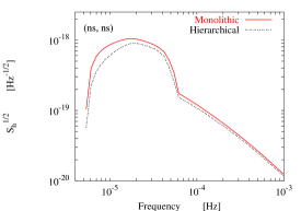
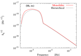
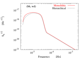
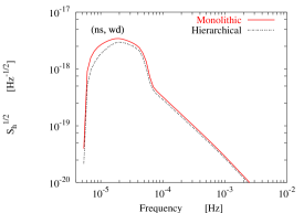
The strain amplitude of the backgrounds has a maximum amplitude between $\sim 10^{-18}\,\mbox{Hz}^{-1/2}$ and $\sim 5\times 10^{-17}\,\mbox{Hz}^{-1/2}$ at frequencies in the interval $[\sim 5\times 10^{-6}-5\times 10^{-5}]$ Hz. The function $S_{h}$ is more sensitive to the low frequency part of the energy density. Therefore, its shape reflects mainly the primary components of the corresponding energy density. In all but the (bh, bh) population, it is evident the presence of a tail at frequencies above the maximum which is the secondary component of the energy density: in the next section we compare this part of the background signal with the LISA sensitivity to assess the possibility of a detection. Still, it is clear that the prominent part of the background signals produced by extragalactic populations of degenerate binaries could be observed with a detector sensitive to smaller frequencies than LISA.

Conversely, $\Omega_{gw}\,h^{2}$ is mostly dominated by secondary components. We can compare the predictions for (bh, bh), (wd, wd) and (ns, ns) systems. Contrary to what has been found for the spectral energy density or for the strain amplitude of the signal, the largest $\Omega_{gw}\,h^{2}$ is produced by (ns, ns), as a consequence of the high amplitude of the secondary component. In particular, no significant contribution from the primary component appears. For (wd, wd), instead, the contribution of the primary component is relevant, although its amplitude is roughly half that of the secondary component. Finally, for (bh, bh) no secondary component is produced and thus the amplitude of the closure density is very low and at very low frequencies. Mixed binary types have different properties, depending on the relative importance of the above effect. For instance, (bh, wd) produce a secondary component but the amplitude is so small to be comparable with that of the primary.

We stress that the value of $\nu_{max}$ is quite uncertain as it defines the boundary between the early inspiral phase and the highly non-linear merger. Clearly, the more we get closer to this boundary, the less accurate is the Newtonian description of the orbit as post-Newtonian terms start to be relevant. Therefore, we believe that the most reliable part of the binary background signal is the low frequency part, i.e. the part which mostly contributes to the strain amplitude $S_{h}$.

Figure 11: The function $\Omega_{gw}\,h^{2}$ of the gravitational background produced by various extragalactic populations of degenerate binaries in monolithic and hierarchical scenarios assuming a flat cosmological background model with zero cosmological constant.

5 Confusion noise level and detectability by LISA

To have some confidence in the detection of a stochastic gravitational background with LISA it is necessary to have a sufficiently large SNR. The standard choice made by the LISA collaboration is $\mbox{SNR}=5$ which, in turn, yields a minimum detectable amplitude of a stochastic signal of (see Bender 1998 and references therein),

$$h^{2}\,\Omega_{gw}[\nu=1\,\mbox{mHz}]\simeq 10^{-12}.$$ (20)

This value already accounts for the angle between the arms ($60^{\circ}$) and the effect of LISA motion. It shows the remarkable sensitivity that would be reached in the search for stochastic signals at low frequencies. Table 2 shows that the backgrounds generated by (wd, wd) and (ns, ns) extragalactic binary populations exceed this minimum value and LISA might be able to detect these signals.

$\nu=$1 mHz	(wd, wd)	(ns, ns)
$\Omega_{gw}\,h^{2}$	$6\times 10^{-12}$	$1.1\times 10^{-12}$

Table 2: The values of the closure density at 1 mHz obtained for (wd, wd) and (ns, ns) extragalactic binary populations investigated. All these values are larger than the minimum detectable value of $\Omega_{gw}\,h^{2}(1\mbox{mHz})$ predicted by the LISA team for a $\mbox{SNR}=5$ and after 1 year of observation.

We plot in Fig. 12 the predicted sensitivity of LISA to a stochastic background after 1 year of observation (Bender 1998). On the vertical axis it is shown $h_{\mbox{rms}}$, defined as,

$$h_{\mbox{rms}}=[2\,\nu\,S_{n}(\nu)]^{1/2}\,\left(\frac{\Delta\nu}{\nu}\right)^{1/2}$$ (21)

where $S_{n}(\nu)$ is the predicted spectral noise density and the factor $(\Delta\nu/\nu)^{1/2}$ is introduced to account for the frequency resolution $\Delta\nu=1/T$ attained after a total observation time $T$.
On the same plot we show the equivalent $h_{\mbox{rms}}$ levels predicted for different extragalactic binary populations and for the galactic population of close white dwarfs binary considered by Bender & Hils (1997).

Figure 12: The sensitivity of LISA to a stochastic background of gravitational waves after one year of observation. The extragalactic backgrounds from (wd, wd), (ns, ns), (ns, wd) and (bh, ns) systems might be observable at frequencies between $\sim 1$ and $\sim 10$ mHz.

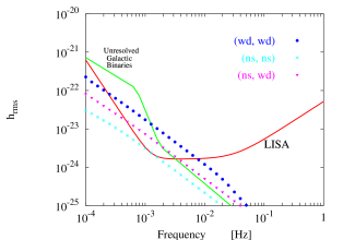
We see that the extragalactic backgrounds might be observable at frequencies between $\sim 1$ and $\sim 10$ mHz.

These background signals represent additional noise components to the LISA sensitivity curve when searching for signals from individual sources.

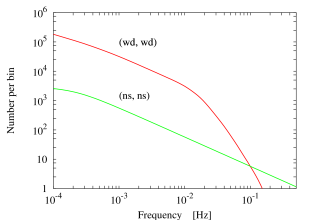
In particular, backgrounds from unresolved astrophysical sources represent a confusion limited noise. In fact, unless the signal emitted by an individual source has a much higher amplitude, the background signal prevents the individual source to be resolved. Clearly, the magnitude of this effect depends on the frequency resolution of the instrument, i.e. on the observation time. The $h_{\mbox{rms}}$ noise levels produced by extragalactic compact binaries shown in Fig. 12 have been computed assuming $T=1$ yr. For the same total observation time we show, in Fig. 13, the number of extragalactic (wd, wd) and (ns, ns) observed in each frequency resolution bin. At frequencies were these backgrounds might be relevant (between 1 and 10 mHz), the number of sources per bin is $\gg 1$, representing a relevant confusion limited noise component. The critical frequency above which the number of sources per bin is lower than 1 occurs at $\sim 0.1$ Hz for (wd, wd) and outside LISA sensitivity window for (ns, ns). However, at these frequencies the dominant noise component is the instrumental noise.

Figure 13: The number of extragalactic (wd, wd) and (ns, ns) binaries per resolution bin after a total observation time of 1yr.

6 Conclusions

In this paper we have obtained estimates for the stochastic background of gravitational waves emitted by cosmological populations of compact binary systems during their early-inspiral phase.

Since we have restricted our investigation to frequencies well below the frequency emitted when each system approaches its last stable circular orbit, we have characterized the single source emission using the quadrupole approximation.

Our main motivation was to develop a simple method to estimate the gravitational signal produced by populations of binary systems at extragalactic distances. This method relies on three main pieces of information:

1. the theoretical description of gravitational waveforms to characterize the single source contribution to the overall background

2. the predictions of binary population synthesis codes to characterize the distribution of astrophysical parameters (masses of the stellar components, orbital parameters, merger times etc.) among each ensemble of binary systems

3. a model for the evolution of the cosmic star formation history derived from a collection of observations out to $z\sim 5$ to infer the evolution of the birth and merger rates for each binary population throughout the Universe.

As we have considered only the early-inspiral phase of the binary evolution, our predictions for the resulting gravitational signals are restricted to the low frequency band $10^{-5}-1$ Hz. The stochastic background signals produced by (wd, wd) and (ns, ns) might be observable with LISA and add as confusion limited noise components to the LISA instrumental noise and to the signal produced by binaries within our own Galaxy. The extragalactic contributions are dominant at frequencies in the range $1-10$ mHz and limit the performances expected for LISA in the same range, where the previously estimated sensitivity curve was attaining its mimimum.

We plan to extend further this preliminary study and to consider more realistic waveforms so as to enter a frequency region interesting for ground-based experiments.

Finally, in Fig. 14 we show the spectral densities of the extragalactic backgrounds that have been investigated so far. The high frequency band appears to be dominated by the stochastic signal from a population of rapidly rotating neutron stars via the r-mode instability (see FMSII). For comparison, we have shown the overall signal emitted during the core-collapse of massive stars to black holes (see FMSI). In this case, the amplitude and frequency range depend sensitively on the fraction of progenitor star which participates to the collapse. The signal indicated with BH corresponds to the conservative assumption that the core mass is $\sim 10\%$ of the progenitor’s (see FMSI). Recent numerical simulations of core-collapse supernova explosions (Fryer 1999) appear to indicate that for progenitor masses $>40M_{\odot}$ no supernova explosion occurs and the star directly collapses to form a black hole. The final mass of this core depends strongly on the relevance of mass loss caused by stellar winds (Fryer & Kalogera 2000). If massive black holes are formed the resulting background would have a larger amplitude and the relevant signal would be shifted towards lower frequencies, more interesting for ground-based interferometers (Schneider, Ferrari & Matarrese 1999).

In the low frequency band, we have plotted only the backgrounds produced by (bh, bh), (ns, ns) and (wd, wd) binaries because their signals largely overwhelm those from other degenerate binary types.

Figure 14: The predicted strain amplitude of the stochastic backgrounds produced by extragalactic populations of gravitational sources. In the high frequency band, we show the estimates for the background produced by rotating neutron stars via r-mode instability, and two possible signals emitted by populations of massive stars collapsing to black holes (see text). In the low frequency band, we plot the background predicted for three different populations of binary systems.

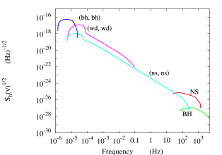
We find that both in the low and in the high frequency band, extragalactic populations generate a signal which is comparable to and, in some cases, larger than the backgrounds produced by populations of sources within our Galaxy (Giazotto, Bonazzola & Gourgoulhon 1997; Giampieri 1997; Postnov 1997; Hils, Bender & Webbink 1990; Bender & Hils 1997; Postnov & Prokhorov 1998; Nelemans, Portegies Zwart & Verbunt 1999). It is important to stress that even if future investigations reveal that the amplitude of galactic backgrounds might be higher than presently conceived, their signal could still be discriminated from that generated by sources at extragalactic distance. In fact, the signal produced within the Galaxy shows a characteristic amplitude modulation when the antenna changes its orientation with respect to fixed stars (Giazotto, Bonazzola & Gourgoulhon 1997; Giampieri 1997).

The same conclusions can be drawn when the extragalactic backgrounds are compared to the stochastic relic gravitational signals predicted by some classical early Universe scenarios. The relic gravitational backgrounds suffer of the many uncertainties which characterize our present knowledge of the early Universe. According to the presently conceived typical spectra, we find that their detectability might be severely limited by the amplitude of the more recent astrophysical backgrounds, especially in the high frequency band.

References

- [1] Abt H.A., Levy S.G., 1978, ApJSS, 36, 241
- [2] Bender P. L. & Hils D., 1997, Class. Quant. Gravity, 14, 1439
- [3] Bender P.L. for the LISA SCIENCE TEAM, 1998, LISA Pre-Phase Report, second edition
- [4] Calzetti D., 1997, AJ 113, 162
- [5] Calzetti D., Heckman T. M., 1999, ApJ, 519, 27
- [6] Carraro G., Chiosi G., 1994, A&A, 287, 761
- [7] Cappellaro E., Turatto M., Tsvetkov D.Y., Bartunov O.S., Pollas C., Evans R., Hamuy M., 1997, A&A, 322,431
- [8] Connolly A.J., Szalay A.S., Dickinson M., SubbaRao M.U., Brunner R.J., 1997, ApJ, L11
- [9] Cutler C. et al. , 1993, Phys. Rev. Lett., 70, 2984
- [10] Damour T., Iyer B.R., Sathyaprakash B.S., 1998, in the Second Amaldi Conference on Gravitational Waves, E. Coccia, G. Pizzella, G. Veneziano eds., (World Scientific, Singapore)
- [11] Danzmann K. for the LISA Study Team, 1997, Class. Quant. Gravity, 14, 1399
- [12] Duquennoy A., Mayor M., 1991, A&A, 248, 485
- [13] Ellis R.S., 1997, A.R.A.A., 35, 389
- [14] Ferrari V., Matarrese S., Schneider R., 1999a, MNRAS, 303, 247 (FMSI)
- [15] Ferrari V., Matarrese S., Schneider R., 1999b, MNRAS, 303, 258 (FMSII)
- [16] Fixsen D.J., Dwek E., Mather J.C., Bennett C.L., Shafer R.A.,1998, ApJ, 508, 123
- [17] Flanagan E.E. & Hughes S.A., 1998, Phys. Rev. D57, 4535
- [18] Flores H., Hammer F., Thuan T.X., Césarsky C., Desert F.X., Omont A., Lilly S.J., Eales S., Crampton D. and Le Févre O., 1999, 517, 148
- [19] Fryer C.L., 1999, ApJ, 522, 413
- [20] Fryer C.L., Kalogera V., 2000, submitted to ApJ, pre-print (astro-ph/9911312)
- [21] Gallego J., Zamorano J., Arágon-Salamanca A., Rego M., 1995, ApJ, 455, L1
- [22] Giampieri G., 1997, MNRAS, 292, 218
- [23] Giazotto A., Bonazzola S., Gourgoulhon E., 1997, Phys. Rev. D55, 2014
- [24] Glazebrook K., Blake C., Frossie E., Lilly S., Colless M., 1999, MNRAS, 306, 843
- [25] Gronwall, 1999, After the Dark Ages: When Galaxies were Young (the Universe at ), 9th Annual October Astrophysics Conference in Maryland, S. Holt, E. Smith eds., American Institute of Physics Press, pg. 335
- [26] Hartman J.W., Bhattacharya D., Wijers R.A.M.J.,Verbunt F., 1997, A&A, 322, 477
- [27] Hils D.L., Bender P., Webbink R.F., 1990, ApJ, 360, 75
- [28] Hughes D. H. and the UK Submillimeter Survey Consortium, 1998, Nature, 394, 241
- [29] Kidder L.E., Will C.M., Wiseman A.G., 1993, Phys. Rev. D47, 3281
- [30] Kosenko, D.I. & Postnov, K.A., 1998, A&A, 336, 786
- [31] Kraicheva, Z.T., Popova, E.I., Tutukov, A.V., Yungelson, L.R., 1978, AZh. 55, 1176
- [32] Langer, N., Hamann, W. R., Lennon, M., et al. Najarro, F., Pauldrach, A. W. A., Puls, J. 1994, A&Ap 290, 819
- [33] Lilly S.J., Le Févre O., Hammer F., Crampton D., 1996, ApJ, 460, L1
- [34] Lipunov V.M., Nazin S.N., Panchenko I.E., Postnov K.A., Prokhorov M.E., 1995, A&A, 298, 677
- [35] Lipunov V.M., 1997, invited review at the XXIII General Assembly of IAU “High Energy Transients”, Kyoto, 1997 pre-print (astro-ph/9711270).
- [36] LISA: Jafry, Y. R., Cornelisse, J., Reinhard, R., 1994, ESA Journal (ISSN 0379-2285), vol. 18, no. 3, p. 219-228
- [37] Madau P., Ferguson H.CC., Dickinson M.E., Giavalisco M., Steidel C.C., Fruchter A., 1996, MNRAS, 283, 1388
- [38] Madau P., Pozzetti L., Dickinson M., 1998a, ApJ, 498, 106
- [39] Madau P., Della Valle M., Panagia N., 1998b, MNRAS, 297, L17
- [40] Mao S., Yi I., 1994, ApJ, 424, L131
- [41] Meynet G., Mermilliod J.C., Maeder A., 1993, A&AS, 98, 477
- [42] Mironovskij V.N., 1966, Sov. Astr.- AJ, 9 752
- [43] Misner C. W., Thorne K. S., Wheeler J.A., Gravitation, Nineteenth printing, 1995, W.H. Freeman & Co., New York
- [44] Narayan, R., Piran, T., Shemi, A., 1991, ApJ 379, L17–21
- [45] Nauenberg, M., 1972, ApJ, 175, 417
- [46] Nelemans G., Portegies Zwart S.F. & Verbunt F., 1999, to appear in the proceedings of the XXXIVth Rencontres de Moriond on ”Gravitational Waves and Experimental Gravity”, pre-print (astro-ph/9903255)
- [47] Paczyński B., 1986, ApJ, 308, L43
- [48] Paczyński B., 1990, ApJ, 348, 485
- [49] Pain R., et al. 1997, ApJ, 473, 356
- [50] Pei Y.C., Fall S.M., 1995, ApJ, 454, 69
- [51] Pei Y.C., Fall S.M., Hauser M.G., 1999, ApJ, 522, 604
- [52] Perlmutter S., et al. 1998, Nature, 391, 51
- [53] Peters, Mathews, 1963, Phys. Rev., 131, 435
- [54] Piran E.S., 1996, in Compact stars in binaries, ed. J. van Paradijs, E.P.J. van den Heuvel, E. Kuulkers (Dordrecht: Kluwer), p. 489
- [55] Portegies Zwart S.F. & Verbunt F., 1996, A&A, 309, 179
- [56] Portegies Zwart, S.F. & Yungelson, L.R., 1998, A & A 332, 173
- [57] Portegies Zwart, S.F. & Yungelson, L.R., 1999, MNRAS, 309, L26
- [58] Portegies Zwart, S.F. & McMillan S.L.W., 1999, ApJ in press
- [59] Postnov, K.A. & Prokhorov, M.E., 1998, ApJ 494, 674
- [60] Rasio, F.A., Shapiro, S.L., 2000, invited Topical Review to appear in Classical and Quantum Gravity, pre-print (gr-qc/9902019)
- [61] Rosi, L.A., Zimmermann, R.L., 1976, ApJSS 45, 447
- [62] Scalo, J.M., 1986, Fund. of Cosm. Phys. 11,1
- [63] Schneider R., Ferrari V., Matarrese S., 1999, in preparation
- [64] Steidel C.C., Giavalisco M., Pettini M., Dickinson M., Adelberger K.L., 1996, ApJ, 462L, 17
- [65] Steidel C.C., Adelberger K.L., Giavalisco M., Dickinson M., Pettini M., 1999, ApJ, 519, 1
- [66] Tammann G.A., Löffler W., Schröder A., 1994, ApJS, 92, 487
- [67] Treyer, M.A., Ellis, R.S., Milliard, B., Donas, J., Bridges, T.J., 1998, MNRAS 300,303
- [68] Tresse L., Maddox S.J., 1998, ApJ, 495, 691
- [69] van den Bergh, S., Tamman, G.A., 1991, ARA&A 29, 363
- [70] van den Heuvel, E.P.J., Lorimer, D.R., 1996, MNRAS 283, L37
- [71] van den Hoek, B., 1997, PhD Thesis, U. Amsterdam
- [72] van den Hoek, B., de Jong, T., 1997, A&A 318, 231