Stringent Tests of Gravity with Highly Relativistic Binary Pulsars in the Era of LISA and SKA

Abstract

At present, 19 double neutron star (DNS) systems are detected by radio timing and 2 merging DNS systems are detected by kilo-hertz gravitational waves. Because of selection effects, none of them has an orbital period $P_{b}$ in the range of a few tens of minutes. In this paper we consider a multimessenger strategy proposed by Kyutoku et al. (2019), jointly using the Laser Interferometer Space Antenna (LISA) and the Square Kilometre Array (SKA) to detect and study Galactic pulsar-neutron star (PSR-NS) systems with $P_{b}\sim$ 10–100 min. We assume that we will detect PSR-NS systems by this strategy. We use standard pulsar timing software to simulate times of arrival of pulse signals from these binary pulsars. We obtain the precision of timing parameters of short-orbital-period PSR-NS systems whose orbital period $P_{b}\in(8,120)\,$min. We use the simulated uncertainty of the orbital decay, $\dot{P}_{b}$, to predict future tests for a variety of alternative theories of gravity. We show quantitatively that highly relativistic PSR-NS systems will significantly improve the constraint on parameters of specific gravity theories in the strong field regime. We also investigate the orbital periastron advance caused by the Lense-Thirring effect in a PSR-NS system with $P_{b}=8\,$min, and show that the Lense-Thirring effect will be detectable to a good precision.

1 Introduction

Currently, general relativity (GR) is the best tested theory of gravity and has passed all the tests with flying colors (Will, 2014). But there are tentative alternative theories that could possibly explain the “missing mass” problem in galaxies and the accelerating expansion of our Universe without introducing dark matter or dark energy (Jain & Khoury, 2010; Clifton et al., 2012). In addition, there are theoretical arguments that GR may not be the exactly correct gravity theory in the ultraviolet end, and it is necessary to test GR and alternative theories more precisely. There are many gravity tests in the Solar System and these tests provide very tight restriction on the parameter space of theories beyond GR. Great achievements were made in bounding the parametrized post-Newtonian (PPN) parameters (Will, 2018). Because different theories of gravity correspond to different values of PPN parameters in the weak field, bounding PPN parameters can help us test theories of gravity in a systematic way. The Solar System experiments probe gravitation in the weak field regime. However, for some gravity theories, such as the scalar-tensor gravity of Damour & Esposito-Farèse (1993), gravity can be reduced to GR in the weak field, while it is very different from GR in the strong field (Damour & Esposito-Farèse, 1992, 1996; Shao & Wex, 2016). So testing theories of gravity in the strong field can help us understand gravity theory more comprehensively.

Radio pulsars, rotating neutron stars (NSs) with radio emission along their magnetic poles, are ideal astrophysical laboratories for strong-field gravity tests, because of the strong self-gravity of NSs. Binary pulsar systems, in which one or more bodies are NSs, provide us an opportunity to test gravity in the strong field. We can measure the parameters of binary pulsar systems with very high precision, which benefits from an extremely accurate measurement technology, the so-called pulsar timing (Lorimer & Kramer, 2005; Wex, 2014). Pulsar timing precisely measures the times of arrival (TOAs) of radio signals at the telescope on the Earth and fits an appropriate timing model to these TOAs to get a phase-connected solution. In 1974, Hulse & Taylor (1975) discovered the first binary pulsar system, PSR B1913+16, which is a double NS (DNS) system. This system proved the existence of gravitational wave (GW) radiation for the first time (Taylor et al., 1979), using the fact that the observed orbital period decay rate, $\dot{P}_{b}^{\rm obs}$, is consistent with the predicted value from GR, $\dot{P}_{b}^{\rm GR}$. With more and more binary systems discovered, we can use them to test a variety of theories of gravity (see e.g. Manchester, 2015; Kramer, 2016; Shao & Wex, 2012, 2013; Shao et al., 2013; Shao, 2014a, b; Miao et al., 2020; Xu et al., 2020, 2021). For example, $\dot{P}_{b}$ of binary pulsar systems can be used to restrict the time variation of the gravitational constant $G$ (Wex, 2014; Zhu et al., 2019); it can also be used to bound the mass of graviton in massive graviton theories (Finn & Sutton, 2002; Miao et al., 2019; Shao, 2021).

At present, more than 300 binary pulsar systems have been discovered (Manchester et al., 2005), including pulsar-NS (PSR-NS) systems, pulsar-white dwarf (PSR-WD) systems, pulsar-main sequence star (PSR-MS) systems and so on. Among them, PSR-NS systems are ideal to test gravity theory, because most pulsars in these systems are millisecond pulsars (MSPs) which come from the “reversal mechanism” (namely, the so-called “recycled pulsars”; Tauris et al., 2017). MSPs are generally more precise timers than normal pulsars, because the timing precision of normal pulsars are usually dominated by red noise, spin irregularities, glitched, etc. (Lyne et al., 2010). Therefore MSPs can provide more precise gravity tests.

Up to now, 19 DNS systems have been discovered from radio telescopes (Manchester et al., 2005). One of them is a double pulsar system, PSR J0737$-$3039A/B (Kramer et al., 2006), which provides a wealth of relativistic tests. The DNS system with the shortest orbital period is PSR J1946+2052 with ${P}_{b}=0.078\,{\rm day}$, and this system has the largest periastron advance, $\dot{\omega}=25.6\pm 0.3\,{\rm deg\,yr^{-1}}$ (Stovall et al., 2018). Binary pulsar systems with shorter orbital periods can provide more relativistic gravity tests because of higher relative velocity $v$. They also can provide smaller fractional uncertainties for some binary orbital parameters. For example, the expected dependence of fractional uncertainty of $\dot{P}_{b}$ is proportional to $P_{b}^{3}$ (Damour & Taylor, 1992; Lorimer & Kramer, 2005). So in most cases shorter orbital period PSR-NS systems can help us test gravity better. But we have not detected DNS systems with orbital periods of several minutes by radio observation yet, because the fast-changing Doppler shift caused by orbital acceleration of the pulsar can smear the pulsar signal in the Fourier domain. Therefore, the selection effect makes the detection of pulsars in very tight binary systems difficult (Tauris et al., 2017).

In addition to radio observations, GW observations from LIGO/Virgo have also detected two DNS systems, GW170817 in the second observing run (O2; Abbott et al., 2017) and GW190425 in the third observing run (O3; Abbott et al., 2020). Because of the high frequency range of LIGO and Virgo, we can only detect GWs from DNS systems near their phase of merger. Therefore, the orbital period of the discovered DNSs has a gap between 1.88 hr (PSR J1946+2052) and $\sim 1\,$ms at the phase of merger. If we can detect a DNS system with an orbital period in this gap, it can help us better understand the population and formation mechanism of DNS systems. On the other hand, these systems with orbital periods of several minutes are highly relativistic, so they can provide complementary gravity tests to what have been done with current pulsar and GW observations.

In 2018, Kyutoku et al. (2019) proposed a multimessenger strategy, combining the Laser Interferometer Space Antenna (LISA) and the Square Kilometre Array (SKA), to detect radio pulses from Galactic DNSs with a period shorter than 10 minutes. LISA is a future space-based GW detector, and it is sensitive at mHz bands (Amaro-Seoane et al., 2017), which makes DNS systems with ${P}_{b}\sim\,$min a target for detection. SKA (Phase 2) under construction will greatly improve detection sensitivity of radio observation in the future. According to the schedule, LISA and SKA will perform their missions simultaneously for a duration of time. Kyutoku et al. (2019) considered that we can utilize LISA to discover DNS systems, and provide their sky location and binary parameters with a high accuracy. Then one can use SKA to probe whether or not a visible pulsar exists in the DNS system. The sky location information can help SKA locate the DNS, and the information of binary parameters can help recover pulse signals modulated by orbital motion. With the help of LISA, SKA can detect PSR-NS systems with ${P}_{b}\sim\,$min more easily with affordable computational cost. So to some extent, the multimessenger strategy can help us reduce the difficulty in searches of short-orbital-period PSR-NS systems.

As a future high-sensitivity radio instrument, SKA can improve the measurement precision of TOAs of pulse to an unprecedented level, which can help improve the measured accuracy of binary pulsar parameters. The high precision binary parameters can further help us improve gravity tests. The theoretically projected relation between $P_{b}$ and the fractional error of $\dot{P}_{b}$ in measurement is $\delta(\dot{P}_{b})\propto P_{b}^{3}$ (Lorimer & Kramer, 2005). So for the short-orbital-period PSR-NS systems, $\delta(\dot{P}_{b})$ can be well measured. Then we can use the high precision $\dot{P}_{b}$ to provide tighter bounds on the parameter space of gravity theories beyond GR.

In general, short-orbital-period binary pulsars are short lived. Recent literature have estimated the number of DNS systems that can be detected by LISA. Based on different Galaxy DNS merger rates, Andrews et al. (2020) considered that LISA will detect on average 240 (330) DNS systems in the Galaxy for a 4-yr (8-yr) mission with signal to noise ratio (SNR) above 7. Lau et al. (2020) estimated that around 35 DNSs will accumulate SNR$\,>8$ over a 4-yr LISA mission. Although the estimated number for DNSs to be detected by LISA are different in the above two papers, they all confirm that a certain number of DNS systems are likely to be detected by LISA. Therefore, we expect that the multimessenger strategy can detect short-orbital-period PSR-NS systems in the future.

In this work, we assume that in the future some short-orbital-period PSR-NS systems are detected by the multimessenger strategy. Based on this assumption, we simulate the fractional error of parameters of these short-orbital-period PSR-NS systems using the standard pulsar timing software TEMPO2, and use the simulated precision of the parameter $\dot{P}_{b}$ to constrain specific theories of gravity, including varying-$G$ theory, massive gravity and scalar tensor theories. Results of our simulation show significant improvement in the constraints of specific parameters of gravity theories in the strong field. We also provide a simple estimate of orbital periastron advance rate, $\dot{\omega}_{\rm LT}$, due to the Lense-Thirring effect. Our result suggests that we are able to measure the value of $\dot{\omega}_{\rm LT}$ in the short-orbital-period PSR-NS systems, which can help us restrict the equations of state (EOSs) of NSs. We need to underline that we have ignored higher order contributions in our simulation, thus our results are indicative, but providing a reasonable estimate of the magnitude of the precision of parameters.

The paper is organized as follows. In the next section, we overview the multimessenger strategy and list the estimated number of DNSs which could be detected by LISA from several work. In Sec. 3, we simulate the parameters of PSR-NS systems to be detected by the joint observation of LISA and SKA. We give the simulated fractional uncertainty of parameters. In Sec. 4, we use our simulated fractional uncertainty of the parameter $\dot{P}_{b}$ to constrain parameter spaces of some specific theories of gravity. In Sec. 5, we provide an estimate on the order of magnitude of orbital periastron advance rate, $\dot{\omega}_{\rm LT}$. Finally we give a discussion in Sec. 6.

2 Observing DNSs with LISA and SKA

At present, the detected DNS system of the shortest orbital period is PSR J1946+2052 with $P_{b}=0.078\,{\rm day}$ (Stovall et al., 2018). The merging timescale is provided by (Peters, 1964; Liu et al., 2014),

$$T_{\rm merge}=\frac{5}{256}\left(\frac{P_{b}}{2\pi}\right)^{8/3}T_{\odot}^{-5/3}\frac{(m_{p}+m_{c})^{1/3}}{m_{p}m_{c}}G(e)\,,$$ (1)

where

$$G(e)=1-3.6481e^{2}+5.1237e^{4}-3.5427e^{6}+1.3124e^{8}+\cdots\,.$$ (2)

In Eq. (1), $T_{\odot}\equiv GM_{\odot}/c^{3}\approx 4.9254909\,{\rm\mu s}$ where $M_{\odot}$ is the Solar mass, $m_{p}$ and $m_{c}$ are the masses of the pulsar and the companion in Solar units respectively, and $e$ is the eccentricity of the binary system. By calculating Eq. (1), we get the merging timescale of PSR J1946+2052, $T_{\rm merge}=46\,{\rm Myr}$, which means that this system will take $46\,{\rm Myr}$ to merge. The GW events from DNS merging suggest that the Galactic merger rate of DNSs is about one in $10^{4}\,{\rm yr}$ (Abbott et al., 2017, 2020). So there must be undetected DNS systems with $P_{b}<0.078\,{\rm day}$ in the Galaxy. The reason why we have not observed DNS systems with orbital period less than one hour is that we are constrained by our present searching methods. Radio observations contributed mostly to DNS detection, as 19 DNS systems have been detected by radio telescopes. Orbital motion of the short-orbital-period binary systems can lead to a severe Doppler smearing which makes it difficult for radio observation to recover the pulse signals of such systems. In GW observation, LIGO/Virgo detected two DNS systems, GW170817 in O2 and GW190425 in O3 (Abbott et al., 2017, 2020). However, LIGO/Virgo are only sensitive to the merger phase. Therefore, constrained by the existing technology and observation, currently it is difficult to detect DNS systems with $P_{b}\sim{\rm min}$.

LISA, a future space-based GW detector, which is expected to be operational in 2030s, is sensitive at mHz bands, so the DNS systems with ${P}_{b}\sim{\rm min}$ are potential targets for LISA. Recently, several works have provided estimates of the number of DNS systems that could be detected by LISA. Andrews et al. (2020) used the Galaxy DNS merger rate of $210\,{\rm Myr^{-1}}$, which is derived from Abbott et al. (2017, 2019), to estimate the number of DNSs that LISA could detect. They showed that LISA will detect on average 240 (330) DNS systems in the Galaxy with ${\rm SNR>7}$ for a 4-yr (8-yr) mission. They also used a conservative DNS merger rate, $42^{+30}_{-14}\,{\rm Myr^{-1}}$ (Pol et al., 2019), and estimated that LISA will detect on average 46 (65) DNS systems in the Galaxy for a 4-yr (8-yr) mission with ${\rm SNR>7}$. The smaller merger rate could suffer from a selection effect (Tauris et al., 2017). At the same time, Lau et al. (2020) provided an estimation that around 35 DNSs will accumulate SNR above 8 over a 4-yr LISA mission. They gave a smaller detectable number of DNSs than that in Andrews et al. (2020). It is because that Lau et al. (2020) used a smaller DNS merger rate, $33\,{\rm Myr^{-1}}$. Overall, no matter we use a conservative or an optimistic DNS merger rate, LISA has a high probability of detecting the DNS systems with $P_{b}\sim{\rm min}$, and there may be PSR-NS systems within them.

Kyutoku et al. (2019) provided a multimessenger strategy, using LISA and SKA, to detect PSR-NS systems with $P_{b}\sim 10\,{\rm min}$ in the Galaxy. LISA can detect DNSs with $P_{b}\sim\,{\rm min}$ and provide information on the location and orbital parameters of DNSs. These information can help SKA locate DNS systems and recover the radio pulse signal which could exist in the system (Kyutoku et al., 2019). So the joint observation strategy can significantly reduce the number of trials used to search for DNS systems with radio telescopes alone. Kyutoku et al. (2019) estimated the 1-$\sigma$ statistical errors of parameters when SNR $\rho=200$ for a 2-yr observation mission, and the uncertainties of parameters can be found in their Eqs. (9-11). With the estimated errors of parameters, Kyutoku et al. (2019) showed that LISA can locate DNS within an error range $\Delta\Omega\approx 0.036\,{\rm deg^{2}}$ [see their Eq. (11)] and then SKA only needs to take 240 pointings to locate the DNS system precisely by a tied-array beam. So the multimessenger strategy can greatly reduce the number of points that an all-sky survey needs. After locating the DNS system, we can use the orbital frequency and binary parameters provided by LISA to recover possible pulse signal of the pulsar, which also can greatly reduce the number of required trials when using a coherent integration. We should notice that all-sky survey is not confined to detect PSR-NS systems with $P_{b}\sim 10\,{\rm min}$. It can be used for other radio source searching as well. The multimessenger observation can specifically and efficiently help us detect PSR-NS systems with $P_{b}\sim 10\,{\rm min}$.

Based on Kyutoku et al. (2019), Thrane et al. (2020) offered an extended analysis for the joint detection of LISA and SKA. They considered a 4-yr observation mission of LISA where the SNR can be improved to $\rho=360$, so the fractional errors of parameters can be further reduced. With the improved precision of parameters, we can use the joint detection to detect short-orbital-period PSR-NS systems more efficiently.

In conclusion, with a reasonable merger rate for Galactic DNSs, the joint detection of SKA and LISA can provide an efficient and more targeted way for detecting PSR-NS systems with very short orbital period.

3 Pulsar-timing simulations

The multimessenger strategy can offer a specific approach to seek for the short-orbital-period PSR-NS systems. These systems can provide a more relativistic situation to test gravity. In our paper, we assume that we will have detected PSR-NS systems by this way in the future, and then we simulate the precision of orbital parameters of the short-orbital-period PSR-NS systems for the SKA.

SKA as the next generation radio telescope will enable the precision of TOAs to reach an unprecedented level. Liu et al. (2014) provided approximated measurement precision on TOAs at $1.4\,{\rm GHz}$ with 10-min integration, which is listed in Table 1 of their work. These results are based on the presumed instrumental sensitivities. In practice, the precision of TOAs depends not only on instrumental sensitivities, but also on interstellar medium evolution, intrinsic pulse shape changes, etc. (Liu et al., 2011). Based on various effects, Liu et al. (2011) predicted that a TOA precision of a normal-brightness MSP can achieve $80$–230$\,{\rm ns}$ at $1.4\,{\rm GHz}$ with 10-min integration by the SKA.

The timing precision of young pulsars is normally dominated by red noise, spin irregularities and glitches, etc., so the timing precision could not be significantly improved by increasing the system sensitivity of telescopes. Hence we assume that the pulsar in PSR-NS system is recycled, which has stable precision of TOAs in general, and we use a spin period $P=20\,{\rm ms}$. For simplification, we only consider white noise. In our work, considering the possible contributions of various effects, we use two different measurement precisions of TOAs to perform the simulations, $\sigma_{\rm TOA}=100\,{\rm ns}$ and $\sigma_{\rm TOA}=1\,\mu{\rm s}$. LISA is sensitive to DNS systems with ${P}_{b}\sim 10\,{\rm min}$, so the target of multimessenger observation strategy is mainly PSR-NS systems with ${P}_{b}\sim 10\,{\rm min}$. Meanwhile, radio observation can also provide us opportunity to detect systems with a period around 100 min by “acceleration search” (Johnston & Kulkarni, 1991) and “jerk search” (Bagchi et al., 2013; Andersen & Ransom, 2018). So we simulate PSR-NS systems with $P_{b}\in[8,\,120]\,{\rm min}$. For the masses of the NSs, we choose two sets of parameters, $m_{p}=1.3\,M_{\odot}$, $m_{c}=1.7\,M_{\odot}$ and $m_{p}=1.35\,M_{\odot}$, $m_{c}=1.44\,M_{\odot}$. Andrews et al. (2020) used the equations from Peters (1964) to show how orbits of the 20 known PSR-NSs will evolve over the next 10 Gyr as gravitational radiation causes them to circularize and decay. Figure 1 in Andrews et al. (2020) shows that the orbital eccentricity goes smaller than 0.1 when the orbital period $P_{b}$ of the 20 PSR-NS systems evolve to 10 min. So in our simulation, we set eccentricity $e=0.1$ for the simulation of all systems.

We use the FAKE plug-in in TEMPO2 (Hobbs, 2012) to simulate pulsar timing data. We need to provide a parameter file which contains parameters of the pulsar and binary orbit as input. In this work, we are interested in how the short orbit PSR-NS systems combined with the high-precision measurement of SKA can improve the measurement precision of orbital parameters. Hence, we only consider simulating the time delay of TOAs related to orbital motion. These time delay terms of orbital motion are the R$\rm{\ddot{o}}$mer delay caused by the orbital motion of the pulsar, the Einstein delay caused by the gravitational redshift and the second order Doppler effect, and the Shapiro delay, which is due to the gravitational field of the companion star. For timing model of orbital motion, different models have different orbital parameters to fit. Damour & Deruelle (1986) introduced a phenomenological parametrization, which is called the parametrized post-Keplerian (PPK) formalism, to describe the orbital motion of pulsars. The post-Keplerian (PK) parameters are solutions of the first order post-Newtonian (PN) equations of orbital motion and it is generic for fully conservative gravity theories (Damour & Deruelle, 1985, 1986). In our simulation, we choose the Damour-Deruelle (DD) timing model.

In the DD timing model, we are mainly able to measure 5 PK parameters—$\dot{\omega},\,\gamma,\,r,\,s,\,\dot{P}_{b}$—in binary pulsar systems. In GR, they can be expressed as functions of two component masses (Lorimer & Kramer, 2005),

$$\dot{\omega} =3T_{\odot}^{2/3}\left(\frac{P_{b}}{2\pi}\right)^{-5/3}\frac{1}{1-e^{2}}\left(m_{p}+m_{c}\right)^{2/3}\,,$$ (3)

$$\gamma =T_{\odot}^{2/3}\left(\frac{P_{b}}{2\pi}\right)^{1/3}e\frac{m_{c}\left(m_{p}+2m_{c}\right)}{\left(m_{p}+m_{c}\right)^{4/3}}\,,$$ (4)

$$r =T_{\odot}m_{c}\,,$$ (5)

$$s =\sin i=T_{\odot}^{-1/3}\left(\frac{P_{b}}{2\pi}\right)^{-2/3}x\frac{\left(m_{p}+m_{c}\right)^{2/3}}{m_{c}}\,,$$ (6)

$$\dot{P}_{b} =-\frac{192\pi}{5}T_{\odot}^{5/3}\left(\frac{P_{b}}{2\pi}\right)^{-5/3}f(e)\frac{m_{p}m_{c}}{\left(m_{p}+m_{c}\right)^{1/3}}\,,$$ (7)

with

$$f(e)\equiv\frac{1+(73/24)e^{2}+(37/96)e^{4}}{(1-e^{2})^{7/2}}\,.$$ (8)

In above equations, $x\equiv(a/c)\sin{i}$ is the projected semi-major axis of the pulsar orbit and $i$ is the orbital inclination; $\dot{\omega}$ is the relativistic precession of periastron of pulsar; $\gamma$ is a PK parameter which is related to the Einstein delay; $r$ and $s$ are PK parameters which are related to the Shapiro delay; $\dot{P}_{b}$ is the orbital period decay rate caused by GW quadrupole radiation in GR. For the 5 PK parameters, except that parameters $r$ and $s$ do not depend on $P_{b}$, the expected fractional uncertainty of $\dot{P}_{b}$ is proportional to $P_{b}^{3}$, the expected fractional uncertainty of $\dot{\omega}$ is proportional to $P_{b}$, and the expected fractional uncertainty of $\gamma$ is proportional to $P_{b}^{4/3}$; these dependent relationships are listed in Table II in Damour & Taylor (1992). So PSR-NS systems with $P_{b}\sim 10\,{\rm min}$ can provide better measurement precisions for PK parameters $\dot{P}_{b}$, $\dot{\omega}$ and $\gamma$, which can help us improve the ability of gravity test. In principle, there are extra relativistic PK parameters, e.g., $\delta_{\theta}$. We have omitted them in this work.

Table 1: Parameters of two example PSR-NS systems. Notice that $m_{p}$ and $m_{c}$ are in unit of the Solar mass, as defined in text.

	PSR-NS I	PSR-NS II
$m_{p}$	1.3	1.35
$m_{c}$	1.7	1.44
Eccentricity, $e$	0.1	0.1
Orbital inclination, $i$	$60^{\circ}$	$60^{\circ}$
$\sigma_{\rm TOA}$	$100\,{\rm ns}$ & $1\,\mu{\rm s}$	$100\,{\rm ns}$ & $1\,\mu{\rm s}$

As mentioned previously, we should provide the orbital parameters of PSR-NS systems for the parameter file. We use the parameters of example PSR-NSs listed in Table 1 and Eqs. (3–7) to provide the values of PK parameters. In fact, the PK parameters should be generic, however current measurements of PK parameters in binary pulsars show no significant deviation from the predicted values in GR. In general, we use the error of the observations of PK parameters as a deviation from GR to limit parameter spaces of alternative theories of gravity. Here we assume that GR is correct and predict the bounds on other theories of gravity constrained by these PSR-NS systems.

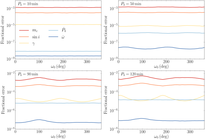
Figure 1: The fractional uncertainties of 5 PK parameters vary with the value of $\omega_{0}$ for different $P_{b}$, given in the upper left corner of each panel. The masses of the simulated PSR-NS system are $m_{p}=1.3\,M_{\odot},~{}m_{c}=1.7\,M_{\odot}$, and we have assumed $\sigma_{\rm TOA}=100\,{\rm ns}$.

We assume a 4-yr observation and ten TOAs per week for the SKA. Ten TOAs per week means that we need to observe a PSR-NS system for 100 min per week, when each TOA is obtained with a 10-min integration time. With parameter file and fitting conditions determined, TEMPO2 can generate simulated TOAs and give a phase-connected solution using the FAKE plug-in by weighted least-squares algorithm (see details, see Hobbs et al., 2006). The simulation can provide values and measurement uncertainties of parameters, and we can utilize the simulated results to predict how the short-period PSR-NS systems can limit specific theories of gravity.

In our simulation, we need to give a value of the longitude of periastron $\omega_{0}$ at the epoch of periastron passage $T_{0}$ in parameter file. Figure 3 of Damour & Taylor (1992) shows that the fractional uncertainties of 5 PK parameters vary with the value of $\omega_{0}$. The reason is that there are some degeneracy between different time delay terms, e.g. Römer delay and Einstein delay, and different values of $\omega_{0}$ can lead to different degrees of degeneracy. Therefore we simulate the fractional uncertainties of 5 PK parameters for different $\omega_{0}$’s. We exhibit results for the “PSR-NS I” system with $\delta_{\rm TOA}=100\,{\rm ns}$ (see Table 1) for different $P_{b}$’s in Fig. 1. As $P_{b}$ increases, different values of ${\omega}_{0}$ can result in a significant difference in the fractional errors of 4 PK parameters, except $\dot{P}_{b}$. So we take the effect of $\omega_{0}$ into account in the simulation and calculate the fractional error with ${\omega}_{0}\in\left[0^{\circ},\,360^{\circ}\right)$.

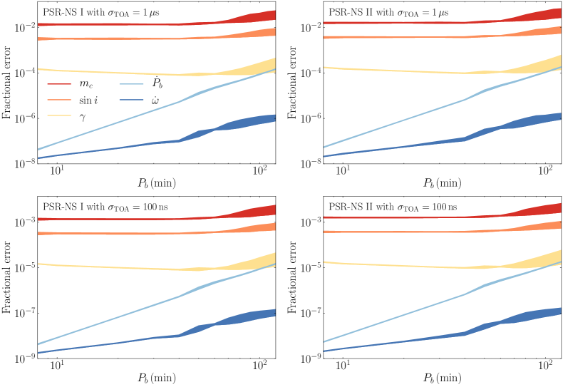
Figure 2: The fractional uncertainties of 5 PK parameters as functions of $P_{b}$. Upper and lower panels are results with $\sigma_{\rm TOA}=1\,{\rm\mu s}$ and $\sigma_{\rm TOA}=100\,{\rm ns}$ respectively. Left and right panels are respectively for PSR-NS I and PSR-NS II (see Table 1). The band in the figure is due to different values of $\omega_{0}$.

Figure 2 shows the fractional uncertainties of 5 PK parameters as functions of $P_{b}$ for a 4-yr observation. The band of the expected fractional uncertainty is caused by simulating with different $\omega_{0}$’s. In the upper panels of Fig. 2, we present the expected measurement precisions of the 5 PK parameters with $\sigma_{\rm TOA}=1\,{\rm\mu s}$. In the lower panels of Fig. 2, we present the results with $\sigma_{\rm TOA}=100\,{\rm ns}$. As shown in Fig. 2, the simulated fractional uncertainties of PK parameters with $\sigma_{\rm TOA}=100\,{\rm ns}$ are an order of magnitude smaller than those with $\sigma_{\rm TOA}=1\,{\rm\mu s}$. SKA can provide a high precision measurement for TOAs of pulsars. The expected sensitivity could be even smaller than 100 ns (Liu et al., 2014), so the precision of PK parameters might be even higher for real detection in the future. At the same TOA precision, the simulated results of the PSR-NS I system are slightly better than that of the PSR-NS II system, which could be caused by a more significant mass difference and thus some reduced degeneracy among parameters.

Based on a 4-yr observation, we notice that the simulated fractional uncertainty of $\dot{P}_{b}$ as a function of $P_{b}$ is largely consistent with what theoretically predicts, namely $\propto P_{b}^{3}$ (Damour & Taylor, 1992; Lorimer & Kramer, 2005). So the predicted fractional uncertainty of $\dot{P}_{b}$ can offer reasonable predictions of gravity tests. The simulated fractional uncertainties of PK parameters $r$ and $s$ are mainly consistent with the theoretical prediction, which are not dependent on $P_{b}$, except that there is a slight rise in $P_{b}\in[40,\,60]\,{\rm min}$. We notice that the slope of PK parameter $\dot{\omega}$ changes significantly in $P_{b}\in[30,\,60]\,{\rm min}$ for a 4-yr observation, which could be caused by the degeneracy between different time delay terms. For parameter $\gamma$ in a 4-yr observation, our simulated results decrease with $P_{b}$ when $P_{b}<60\,{\rm min}$, and then increase with $P_{b}$. So the changing trend of $\delta\left({\gamma}\right)$ is not strictly consistent with the theoretical prediction, $\propto P_{b}^{4/3}$, when $P_{b}<60\,{\rm min}$. For DD model, according to Eqs. (2.2b) and (2.2c) in Damour & Taylor (1992), the Einstein delay is always degenerate with the R$\ddot{\rm o}$mer delay, and the degeneracy depends on the change of relativistic advance of periastron (Liu et al., 2014). So we think that the trend of $\delta\left({\gamma}\right)$ could come from the degeneracy between the R$\ddot{\rm o}$mer delay and the Einstein delay. For PSR-NS systems with $P_{b}\sim 10\,{\rm min}$, they have a large $\dot{\omega}$, and considering a 4-yr observation, their periastrons have precessed several rounds. Hence the periodic change of $\omega$ can not eliminate degeneracy effectively enough and leads to the trend of $\delta\left({\gamma}\right)$ different from the theoretical prediction. For binary systems with $P_{b}>60\,{\rm min}$, the change of $\omega$ is less than $2\pi$, so the trend of $\delta\left({\gamma}\right)$ varying with $P_{b}$ is roughly consistent with the theoretical prediction when considering different values of $\omega_{0}$. So DD model can not avoid the degeneracy because of the specific form of time delay terms, which makes $\gamma$ less well measured when $\Delta{\omega}>2\pi$ in observation.

We have showed the expected fractional uncertainties of PK parameters of short-orbital-period PSR-NS systems which could be detected by LISA and SKA in joint observation in the future. But we need to emphasize that, strictly speaking, the DD timing model is not sufficient to describe the orbital motion of PSR-NS systems with a very short orbital period $P_{b}\sim$ min, because it only takes into account the leading PN order terms. A PSR-NS system with ${P}_{b}=8\,{\rm min}$ is an extremely relativistic system, so, in principle, we need to take high order effects into account in our simulation. Since we mainly use the fractional error of $\dot{P}_{b}$ to test gravity in the following, we provide an extended analysis for $\dot{P}_{b}$. Equation (7) gives the 2.5 PN formula for $\dot{P}_{b}$, $\dot{P}_{b}^{2.5\,{\rm PN}}$, and we actually have appended it with the 3.5 PN contribution (Blanchet & Schaefer, 1989),

$$\delta\dot{P}_{b}^{3.5\,{\rm PN}} =\dot{P}_{b}^{2.5\,{\rm PN}}X^{3.5\,{\rm PN}}\,,$$ (9)

where

$$X^{3.5\,{\rm PN}}= \frac{\left(GmM_{\odot}\right)^{2/3}}{336\left(1-e^{2}\right)c^{2}f(e)}\left(\frac{P_{b}}{2\pi}\right)^{-2/3}$$

$$\times{\bigg{[}}1273+\frac{16495}{2}e^{2}+\frac{42231}{8}e^{4}+\frac{3947}{16}e^{6}$$

$$-\left(924+3381e^{2}+\frac{1659}{4}e^{4}-\frac{259}{4}e^{6}\right)\frac{m_{p}m_{c}}{m^{2}}$$

$$+\left(3297e^{2}+4221e^{4}+\frac{2331}{8}e^{6}\right)\frac{m_{p}-m_{c}}{m}{\bigg{]}}\,.$$ (10)

For a PSR-NS system with $P_{b}=8\,{\rm min},\,e=0.1$, one has $X^{3.5\,{\rm PN}}\sim 1\times 10^{-4}$. Our simulated fractional error of $\dot{P}_{b}$ can reach $10^{-7}$ for $\sigma_{\rm TOA}=1\,\mu{\rm s}$. So, comparing with the simulated fractional error, the contribution from $\delta\dot{P}_{b}^{3.5\,{\rm PN}}$ can be significant for an 8-min system. However $\delta\dot{P}_{b}^{3.5\,{\rm PN}}$ is still a small value relative to $\dot{P}_{b}^{2.5\,{\rm PN}}$, so we use DD timing model to simulate this situation which can give a correct estimate of magnitude of the expected fractional uncertainties of PK parameters, and it can predict the ability of a highly relativistic binary pulsar to test gravity. We hope that we can provide a more suitable timing model to simulate or process TOAs for short-orbital-period PSR-NS systems in future work.

4 Radiative tests of gravity

In this section, we utilize the simulated results of $\dot{P}_{b}$ to do some specific gravity tests. Before we use the fractional error of $\dot{P}_{b}$ to test gravity, we need to emphasize that we should substract the non-intrinsic contibution in $\dot{P}_{b}$ and use the intrinsic value $\dot{P}_{b}^{\rm intr}$ in real gravity test. The value of $\dot{P}_{b}$ from actual pulsar timing is $\dot{P}_{b}^{\rm obs}$ which contains the dynamical contributions from the Shklovskii effect (Shklovskii, 1970) and the differential Galactic acceleration between the Solar System barycenter and the pulsar system (Damour & Taylor, 1991; Lazaridis et al., 2009). So, in general, we need to subtract the contribution of the Shklovskii effect and the Galactic acceleration difference in $\dot{P}_{b}^{\rm obs}$ first via,

$$\left(\frac{\dot{P}_{b}}{{P}_{b}}\right)^{\rm intr}=\left(\frac{\dot{P}_{b}}{{P}_{b}}\right)^{\rm obs}-\left(\frac{\dot{P}_{b}}{{P}_{b}}\right)^{\rm Shk}-\left(\frac{\dot{P}_{b}}{{P}_{b}}\right)^{\rm Gal}\,.$$ (11)

The second term of Eq. (11) is the contribution from the Shklovskii effect which is due to the transverse motion of the pulsar system (Shklovskii, 1970), and the specific form is shown by Eq. (19) in Lazaridis et al. (2009). The third term of Eq. (11) is the contribution from the Galactic acceleration difference (Damour & Taylor, 1991; Lazaridis et al., 2009), and the specific form is given by Eq. (16) in Lazaridis et al. (2009).

The actual fractional error of $\dot{P}_{b}^{\rm intr}$ depends on the errors of $\dot{P}_{b}^{\rm Shk}$ and $\dot{P}_{b}^{\rm Gal}$. So, the fractional errors of $\dot{P}_{b}^{\rm Shk}$ and $\dot{P}_{b}^{\rm Gal}$ will affect gravity tests. In other words, their fractional errors can determine how tight the PSR-NS system can bound the parameter space of non-GR parameters. For $\dot{P}_{b}^{\rm Shk}$ and $\dot{P}_{b}^{\rm Gal}$, their fractional errors all rely on the precision of $D$. At present, we use the Very Long Baseline Interferometry (VLBI) or the dispersion measure (DM) to measure the distance of binary pulsars. For the nearby binary pulsar systems, VLBI can provide an accurate measurement for $D$. Once we have a measured distance with a small error, the errors of $\dot{P}_{b}^{\rm Shk}$ and $\dot{P}_{b}^{\rm Gal}$ could contribute little to the total error and the precision of $\dot{P}_{b}^{\rm intr}$ would largely depend on $\dot{P}_{b}^{\rm obs}$, such as in the case of PSRs J2222$-$0137 (Cognard et al., 2017) and J0737$-$3039 (Kramer et al., 2006). In the opposite case, for remote binary pulsar systems, we can not provide an accurate measurement of $D$ by VLBI or DM. The large uncertainty of $D$ results in large errors of $\dot{P}_{b}^{\rm Shk}$ and $\dot{P}_{b}^{\rm Gal}$, which restrict the precision of $\dot{P}_{b}^{\rm intr}$; for example, see PSR B1913+16 (Weisberg & Huang, 2016; Deller et al., 2018).

So the accurate measurement of the distance of a binary pulsar system helps us reduce the error contribution from astrophysical terms in $\dot{P}_{b}$. Based on a specific DNS system, Kyutoku et al. (2019) provided an estimated fractional uncertainty of distance for a 2-yr mission of LISA,

$$\frac{\Delta D}{D}=0.01\left(\frac{\rho}{200}\right)^{-1}\,.$$ (12)

In Thrane et al. (2020), considering a 4-yr mission of LISA, the fractional uncertainty of distance can reach $0.006$ for a specific DNS system with $\rho=360$. So LISA could improve the accuracy of pulsar distance measurement significantly and then maybe avoid introducing large errors caused by $\dot{P}_{b}^{\rm Shk}$ and $\dot{P}_{b}^{\rm Gal}$ (with a well modelled Galactic potential). Therefore, if LISA can detect a PSR-NS system with a high SNR, it can improve the measure of distance of a PSR-NS system.

To simplify the simulation, we did not include the possible error contribution from $\dot{P}_{b}^{\rm Gal}$ and $\dot{P}_{b}^{\rm Shk}$, so we may derive optimistic results when testing gravity. In Sec. 4.2, to be more complete, we provide a simple calculation for the possible error contribution to $\dot{P}_{b}^{\rm intr}$ from $\dot{P}_{b}^{\rm Shk}$ and $\dot{P}_{b}^{\rm Gal}$, and show the possible impact on gravity tests. We assume LISA can work well in distance measurement, so we use a fractional error of $\Delta D/{D}=0.01$. Actually, $D$ may not be measured with such a high precision, so even if the non-intrinsic effects are considered, the results may still be optimistic because $D$ is assumed to be measured with high precision.

4.1 Theoretical framework

Based on the expected measurement precision of the Five-hundred-meter Aperture Spherical radio Telescope (FAST) and SKA, Liu et al. (2014) simulated the timing precision for black hole-pulsar (BH-PSR) binary systems. Seymour & Yagi (2018) used the simulated parameter precision of $\dot{P}_{b}$ from Liu et al. (2014) to constrain specific gravity theories. In this section, following Seymour & Yagi (2018), we use the simulated precision of $\dot{P}_{b}$ of the short-orbital-period PSR-NS systems to constrain alternative theories of gravity.

In Seymour & Yagi (2018), the authors gave a generic formalism which provides a mapping between generic non-GR parameters in the orbital decay rate $\dot{P}_{b}$ and theoretical constants in various alternative theories of gravity. Details can be found in Table I of Seymour & Yagi (2018). A parameterized non-GR modification to $\dot{P}_{b}$ reads,

$$\frac{\dot{P}_{b}}{{P}_{b}}=\frac{\dot{P}_{b}}{{P}_{b}}\bigg{|}_{\rm GR}\left(1+\Gamma v^{2n}\right)\,,$$ (13)

where $v$ is the relative velocity of two compact objects in a binary system, $v=\left(\frac{2\pi M}{P_{b}}\frac{G}{c^{3}}\right)^{1/3}$, and $M$ is the total mass of binary system. $\left({\dot{P}_{b}}/{{P}_{b}}\right)\big{|}_{\rm GR}$ is the quantity evaluated in GR [cf. Eq. (7)]. $\Gamma$ and $n$ are the non-GR parameters. $\Gamma$ gives the overall magnitude of the correction, and $n$ shows how the correction depends on $v$. In Eq. (13), a correction term proportional to $v^{2n}$ corresponds to a $n$-PN order correction to GR. For different theories of gravity, the non-GR parameter $\Gamma$ corresponds to different forms, which are listed in Table I of Seymour & Yagi (2018), where a specific non-GR theory can be mapped to a set of $(\Gamma,n)$. In our work, we use the same mapping relation to test gravity. We want to estimate how tightly the short-orbital-period PSR-NS systems can constrain the parameters of non-GR theories in the future.

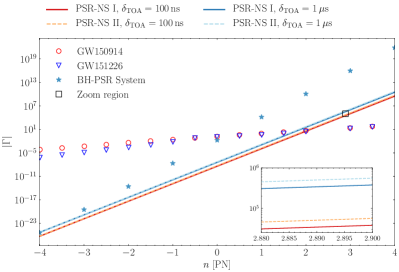
Figure 3: Upper bounds on $\Gamma$ as a function of $n$, where $n$ means that a correction term enters at $n$-PN order relative to GR. We present the predicted constraints with an 8-min PSR-NS system. We provide upper bounds from four sets of simulation: (i) PSR-NS I system with $\delta_{\rm TOA}=100\,{\rm ns}$ (red solid line), (ii) PSR-NS I system with $\delta_{\rm TOA}=1\,{\rm\mu s}$ (blue solid line), (iii) PSR-NS II system with $\delta_{\rm TOA}=100\,{\rm ns}$ (light red dashed line), and (iv) PSR-NS II system with $\delta_{\rm TOA}=1\,{\rm\mu s}$ (light blue dashed line). For comparison, we show bounds from a 3-day PSR-BH system (blue stars; Seymour & Yagi, 2018), and bounds from GW observations with GW150914 and GW151226 (red circle and blue triangle; Yunes et al., 2016). The insert plot is a zoom-in region of the black-squared region.

Following Eq. (4) in Seymour & Yagi (2018), we define a fractional error $\delta$ for the observed ${\dot{P}_{b}}/{{P}_{b}}$, and we can use $\delta$ to bound $\Gamma$ by the following equation,

$$\left|\Gamma\right|<\frac{\delta}{v^{2n}}\,.$$ (14)

In Sec. 3, we have simulated a series of fractional errors of $\dot{P}_{b}$ for different $P_{b}$’s, and these fractional errors of $\dot{P}_{b}$ correspond to the parameter $\delta$ here. Hence we can use the data to predict the constraints on $\Gamma$ for different PN orders.

We choose a PSR-NS system with an 8-min orbital period. Figure 3 presents the predicted upper bounds on $\Gamma$ as a function of PN orders. For comparison, we also present the result from a 3-day orbital period PSR-BH system (Seymour & Yagi, 2018). For a PSR-NS system with an 8-min orbital period, its relative velocity $v$ approximately equals to $5.7\times 10^{-3}$ which is 5 times larger than the velocity of a 3-day orbital period PSR-BH system, whose $v\sim 1\times 10^{-3}$. For negative PN, $\Gamma\propto v^{|2n|}$, so the larger value of $n$, a binary system with a larger $v$ is more disadvantageous for bounding $\Gamma$. For example, if $n=-4$, for an 8-min PSR-NS system, its value of $v^{|2n|}$ is $4\times 10^{5}$ times larger than that of a 3-day PSR-BH system, which greatly reduces the restriction on $\Gamma$. However, the 8-min orbital period PSR-NS system has a smaller fractional error $\delta$, that makes it possible to provide a stronger constraint on $\Gamma$. Combining those two factors, the constraint from an 8-min PSR-NS system is tighter than the constraint from a 3-day PSR-BH system at some negative PN orders, as shown in Fig. 3. At positive PN orders, a larger $v$ is more competitive, so an 8-min PSR-NS system can naturally provide a tighter constraint than a 3-day PSR-BH system. Like Seymour & Yagi (2018), we also show the limits from GW observations in Fig. 3, using GW150914 and GW151226 as examples (Yunes et al., 2016). Because GWs detected by LIGO/Virgo come from the phase of merger, which indicates a larger relative velocity, it leads to a tighter restriction on $\Gamma$ at positive PN orders. But due to the small $\delta$ of the 8-min PSR-NS system, it can give a slightly tighter restriction than GW observations at positive PN order when $n\lesssim 2$.

Overall, the results in Fig. 3 show that the 8-min PSR-NS system can provide a tight bound for the non-GR theories of negative PN orders when $n\gtrsim-4$. However, when comparing these results in a strict way, one should be aware that the prediction may depend on the details of specific theories. NSs and BHs can behave quite differently in alternative gravity theories. We leave this to a future detailed study. In any case, the system that we considered here will provide very useful and complementary constraints. We underline that here the corrections of different PN orders are relative to GR’s quadrupole radiation, not to the equations of motion.

4.2 Projected constraints

In Fig. 3, we show the constraint from an 8-min PSR-NS system on parameter $\Gamma$ as a function of PN orders. In Sec. 4.1, the generic formalism (13) offers a mapping between generic non-GR parameters in the orbital decay rate and theoretical parameters in various alternative theories of gravity (Seymour & Yagi, 2018). We can use this mapping to restrict specific theories of gravity, and then predict how do the short-orbital-period PSR-NS systems constrain these theories.

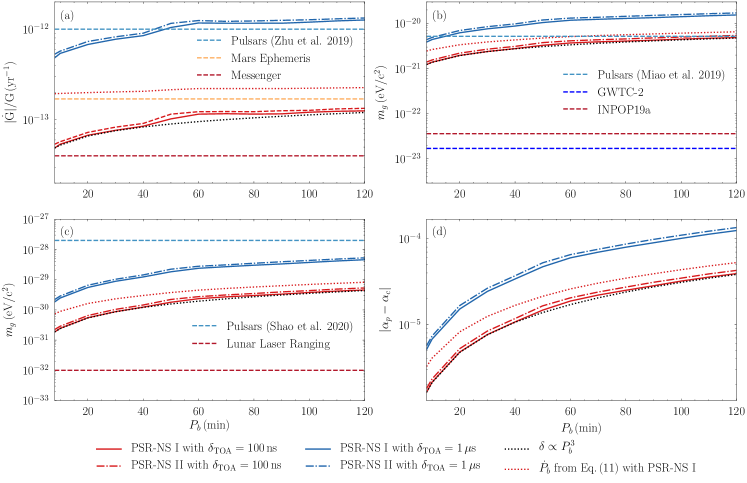
Figure 4: Projected constraints on non-GR parameters with short-orbital-period PSR-NS systems using the SKA. We provide upper bounds from four sets of simulation: (i) PSR-NS I system with $\delta_{\rm TOA}=100\,{\rm ns}$ (red solid line), (ii) PSR-NS I system with $\delta_{\rm TOA}=1\,{\rm\mu s}$ (blue solid line), (iii) PSR-NS II system with $\delta_{\rm TOA}=100\,{\rm ns}$ (red dotted-dashed line), and (iv) PSR-NS II system with $\delta_{\rm TOA}=1\,{\rm\mu s}$ (blue dotted-dashed line). The black dotted line is the trend of bound predicted from theory, i.e., $\delta\propto P_{b}^{3}$ (Damour & Taylor, 1992; Lorimer & Kramer, 2005). The red dotted line is the constraint on non-GR parameters from fractional error of $\dot{P}_{b}^{\rm intr}$ (using PSR-NS I with $\delta_{\rm TOA}=100\,{\rm ns}$ for an illustration) which has taken into account error contributions from $\dot{P}_{b}^{\rm Shk}$ and $\dot{P}_{b}^{\rm Gal}$. Panel (a) shows constraints on $|\dot{G}|/G$ as a function of $P_{b}$ in varying-$G$ theory. For comparison, we show bounds from Solar System: the bound with Mars Ephemeris (Will, 2014) in a gold dashed line, and the bound with NASA Messenger (Genova et al., 2018) in a red dashed line; we also show the constraint from binary pulsars with a blue dashed line (Zhu et al., 2019). Panel (b) shows constraints on graviton mass $m_{g}$ in a Fierz–Pauli-like massive gravity theory. For comparison, the constraint on $m_{g}$ from Solar System (marked “INPOP19a”) is shown in a red dashed line (Bernus et al., 2020); the constraint from GW detection (marked “GWTC-2”) is shown in a blue dashed line (Abbott et al., 2021); the constraint from combination of existing pulsar observations is given in a cyan dashed line (Miao et al., 2019). Panel (c) shows constraints on graviton mass $m_{g}$ in the cubic Galileon massive gravity theory. The latest bound from binary pulsars is shown with a light blue dashed line (Shao et al., 2020). The best bound is from lunar laser ranging experiment (red dashed line; Dvali et al., 2003). Panel (d) shows constraints on $\left|\alpha_{p}-\alpha_{c}\right|$ in DEF gravity theory.

4.2.1 Varying-$G$ theory

In GR, the Newtonian gravitational constant $G$ does not change with time. But in some alternative theories, the locally measured Newtonian gravitational constant $G$ may vary with time, because of the evolution of the Universe (Will, 2014). The gravitational constant which varies with time violates local position invariance, that leads a violation of strong equivalence principle (SEP). Hence proving whether the gravitational constant varies with time helps us test the SEP. If the gravitational constant is changing with time, it can cause changes in the compactness and Arnowitt-Deser-Misner (ADM) mass of a compact star, which would result in an additional contribution to the orbital period decay rate $\dot{P}_{b}$ (Nordtvedt, 1990).

The relation between $\dot{P}_{b}$ and $\dot{G}$ is given by Nordtvedt (1990),

$$\frac{\dot{P}_{b}^{\dot{G}}}{{P}_{b}}=-2\frac{\dot{G}}{G}\left[1-\frac{2m+m_{c}}{2m}s_{p}-\frac{2m+m_{p}}{2m}s_{c}\right]\,,$$ (15)

where $s_{i}$ denotes the “sensitivity” of the NS, which depends on the mass and the EOS of NS,

$$s_{i}\equiv-\frac{\partial\ln{M_{i}}}{\partial\ln{G}},\quad\quad(i=p,c)\,,$$ (16)

where $M_{i}=m_{i}M_{\odot}$ (notice that in this paper $m_{i}$ is the mass in unit of Solar mass). In GR, $s_{i}=0$. We use the value of $s_{i}$ as per Damour & Esposito-Farèse (1992),

$$s_{i}=0.16\,\left(\frac{M_{i}}{1.33M_{\odot}}\right)\,.$$ (17)

With Eqs. (14–15), we get the corresponding expression of $\Gamma$,

$$\Gamma=\frac{5}{48}\frac{\dot{G}}{c^{3}}\frac{m^{3}M_{\odot}}{m_{p}m_{c}}\left[1-\frac{2m+m_{c}}{2m}s_{p}-\frac{2m+m_{p}}{2m}s_{c}\right]\frac{1}{f(e)}\,,$$ (18)

and it is a $-$4 PN order correction relative to GR. So combining Eq. (13) and Eq. (18), we get the upper bound on $\dot{G}$ by,

$$\frac{|\dot{G}|}{G}<-\frac{\delta}{2}\left(\frac{\dot{P_{b}}}{P_{b}}\right)_{\rm GR}{\left(1-\frac{2m+m_{c}}{2m}s_{p}-\frac{2m+m_{p}}{2m}s_{c}\right)^{-1}}\,.$$ (19)

There is an associated dipole radiation of GWs for most gravitational theories that violate SEP. The dipole radiation of GWs can contribute an extra $\dot{P}_{b}^{\rm dipole}$ which is degenerate with $\dot{P}_{b}^{\dot{G}}$. The degeneracy indicates that we need to use multiple binary pulsar systems to break the degeneracy. In our work, for the sake of simplicity, we ignore the possible degeneracy and consider only one violation to GR at a time.

Figure 4 (a) shows the predicted upper limit on $\dot{G}$ from short-orbital-period PSR-NS systems with $P_{b}\in[8,\,120]\,{\rm min}$ to be detected by the SKA. The best bound is $|\dot{G}|/G<4.8\times 10^{-14}\,{\rm yr}^{-1}$ which is from the 8-min PSR-NS I system with $\sigma_{\rm TOA}=100\,{\rm ns}$.

The simulated fractional uncertainty of $\dot{P}_{b}$ varies with $P_{b}$, that is largely consistent with what is theoretically predicted (namely $\delta\propto P_{b}^{3}$; Damour & Taylor, 1992; Lorimer & Kramer, 2005). Because of the degeneracy of some delay terms, there are still slight differences between theoretic prediction and our simulation. In Fig. 4 (a), the black dotted line is the trend by theoretical prediction, $\delta\propto P_{b}^{3}$, and we use PSR-BH I system with $\sigma_{\rm TOA}=100\,{\rm ns}$ to illustrate. Because we show the constraint on $|\dot{G}|/G$, which is a cumulative effect in one year, so there is a noticeable deviation in $P_{b}\in[40,\,60]\,{\rm min}$.

We do not plot the bounds of a PSR-BH system from Seymour & Yagi (2018), and their results are similar to ours. Although the 8-min orbital period system has a very high precision for $\dot{P}_{b}$, as mentioned before, the varying $G$ theory is a $-$4 PN order correction relative to GR. A system with a large $v$ is disadvantageous to provide a tighter bound on $\dot{G}$, so the two systems (PSR-NS and PSR-BH) have similar results.

To provide a more complete analysis, we also consider the fractional error which contains error contributions from $\dot{P}_{b}^{\rm Shk}$ and $\dot{P}_{b}^{\rm Gal}$ to restrict $\dot{G}$ [see Eq. (11)]. We assume that LISA can help us determine the distance of the PSR-NS system very well. So for the fractional error of $D$, we take $0.01$. Considering the error contributions from $\dot{P}_{b}^{\rm Shk}$ and $\dot{P}_{b}^{\rm Gal}$, we show in Fig. 4 (a) the bound from PSR-NS I systems with $\delta_{\rm TOA}=100\,{\rm ns}$ on $\dot{G}$ with the red dotted line. We find that by introducing the errors of $\dot{P}_{b}^{\rm Shk}$ and $\dot{P}_{b}^{\rm Gal}$, our results become worse. Although our distance accuracy is high, the precision of other parameters that we adopt from PSR J0737$-$3039 are low, which prevent us from limiting the non-GR parameters to high precision. If we, likely with the SKA, further improve the measurement accuracy of these parameters in the future, we will constrain $\dot{G}$ better.

In order to compare, we show the current bounds from the Solar System experiments in Fig. 4 (a). We notice that the estimated bound of an 8-min PSR-NS system is slightly weaker than the Solar System result from NASA Messenger (red dashed line; Genova et al., 2018). For now, the best constraint comes from the Solar System experiment, which is from weak field. However, the sensitivity $s_{i}$ is a body-dependent quantity, so it could lead to an enhance of $\dot{G}$ for strongly self-gravitating bodies. NSs are strongly self-gravitating bodies, so it provides the constraint on $\dot{G}$ from a strong field. The constraint on $\dot{G}$ from PSR-NS systems can provide a complementary constraint compared with the constraint from the Solar System experiment. One point that needs to be emphasized is that we can improve the precision of the parameters through long-term observation. For $\dot{P}_{b}$, the expected dependence of fractional uncertainty on observing time, $T_{\rm obs}$, is proportional to $T_{\rm obs}^{-5/2}$. Therefore, according to the theoretical prediction, compared with a 4-yr observation, the measurement precision of $\dot{P}_{b}$ will increase by about 10 times for a 10-yr timing. We simulate a 10-yr timing for PSR-NS I system with $\delta_{\rm TOA}=100\,{\rm ns}$ by using the same cadence, and the result is consistent with the theoretical prediction; that is, the measurement precision is improved by an order of magnitude. Hence, a 10-yr observation could increase the projected limit to $|\dot{G}|/G<5\times 10^{-15}\,{\rm yr}^{-1}$ for an 8-min PSR-NS I system with $\delta_{\rm TOA}=100\,{\rm ns}$. Thus, an 8-min PSR-NS system has the potential to give tighter bound than the present result from the Solar System for $\dot{G}$.

We also provide the previous upper limit on $\dot{G}$ from binary pulsar systems, that combined the results from PSRs J0437$-$4715, J1738+0333, and J1713+0747 (blue dashed line; Zhu et al., 2019). Our simulated results show that the constraint on $\dot{G}$ in strong field can be improved significantly.

4.2.2 Fierz–Pauli-like massive gravity

In GR, gravitation is mediated by a massless spin-2 graviton, and graviton is massless in most theories of gravity. The existence of graviton is not experimentally confirmed yet. There are some theories of gravity where graviton has mass and they cannot be completely ruled out yet. So we can base on different theories to bound graviton mass (de Rham et al., 2017), and we show some results in Fig. 4 (b). If graviton is massive, the gravitational potential possesses an exponential Yukawa suppression. In the Solar System, which can be viewed as a static field, the Yukawa potential can cause planets to behave differently from the Newtonian potential which is $\propto 1/r$. Bernus et al. (2020) used the planetary ephemeris INPOP19a to constrain graviton mass and provided $m_{g}<3.62\times 10\,{\rm eV}/c^{2}$, shown with a red dashed line in Fig. 4 (b). The constraint on $m_{g}$ from the Solar System is a bound in weak field; we also provide two constraints from strong field. The first bound comes from GW data. If gravity is propagated by a massive field, the massive graviton can lead to a modified dispersion relation. In other words, the velocity of the graviton depends on the GW frequency. Using the modified dispersion relation, the LIGO/Virgo Collaboration bound the graviton mass to be $m_{g}<1.8\times 10^{-23}\,{\rm eV}/c^{2}$ by combining the data of 31 GW events from the catalog GWTC-2 (Abbott et al., 2021). This result is represented by a blue dashed line in Fig. 4 (b). This bound coming from the direct detection of GWs is an effect of GWs’ phase accumulation. The second bound is from binary pulsar systems, which is based on a Fierz–Pauli-like massive gravity. Finn & Sutton (2002) presented a phenomenological term in the Lagrangian for linearized gravity with a mass term $\sim m_{g}^{2}\left(h_{\mu\nu}^{2}-\frac{1}{2}h^{2}\right)$ which is similar to the Fierz–Pauli mass term $\sim m_{g}^{2}\left(h_{\mu\nu}^{2}-h^{2}\right)$ (Fierz & Pauli, 1939), but with a different coefficient for $h^{2}$. The choice of this linear mass term ensures that the theory reduces to GR when $m_{g}\rightarrow 0$ [avoiding the van Dam-Veltman–Zakharov (vDVZ) discontinuity] and the derived wave equation takes the standard form (Finn & Sutton, 2002),

$$\left(\square-m_{g}^{2}\right)\bar{h}_{\mu\nu}+16\pi T_{\mu\nu}=0\,,$$ (20)

with an $h$-independent source $T_{\mu\nu}$. We have defined $\bar{h}_{\mu\nu}\equiv h_{\mu\nu}-\frac{1}{2}\eta_{\mu\nu}h$. Finn & Sutton (2002) worked out the relation between $m_{g}$ and $\delta$,

$$m_{g}^{2}<\frac{24}{5}F(e)\left(\frac{2\pi\hbar}{c^{2}P_{b}}\right)^{2}\delta\,,$$ (21)

where $F(e)=f(e)\left(1-e^{2}\right)^{1/2}$ [see Eq. (8) for $f(e)$], and $\hbar$ is the reduced Planck constant. With Eq. (21), we can use binary pulsars to restrict $m_{g}$. Finn & Sutton (2002) provided a method to constrain graviton mass in a dynamic regime. The Fierz–Pauli-like massive gravity gives a $-$3 PN order correction relative to GR. By comparison with Eq. (14), we can obtain the form of $\Gamma$,

$$\Gamma<\frac{5}{24}m^{2}_{g}m^{2}\frac{M_{\odot}^{2}G^{2}}{c^{2}\hbar^{2}}\frac{1}{F(e)}\,.$$ (22)

Finn & Sutton (2002) used PSRs B1913+16 and B1534+12 to bound $m_{g}$. Recently, using 9 well-timed binary pulsars and the Bayesian theorem, Miao et al. (2019) provided an improved bound, $m_{g}<5.2\times 10^{-21}\,{\rm eV}/c^{2}$, which is shown with a light blue dashed line in Fig. 4 (b).

Here, we use the simulated $\delta$ of $\dot{P}_{b}$ of the short-orbital-period PSR-NS systems by the SKA, to predict the constraints on graviton mass. The results of bounds are shown in Fig. 4 (b). The results show that the PSR-NS system with an 8-min short orbital period can give a tighter limit than previous results in Miao et al. (2019) by roughly a factor of 4, $m_{g}<1.2\times 10^{-21}\,{\rm eV}/c^{2}$. Although the projected bounds from PSR-NS systems are looser than the bounds from GWs and the Solar System, they reflect a dynamical process of two compact objects and a strong field effect. The constraint from GWs is based on a modified dispersion relation which is an effect of accumulation in GW phases, so it is a kinematic effect from propagation. The constraint from the Solar System reflects an effect from a static weak field. Hence the restrictions from the binary pulsars are complementary to these constraints. For an 8-min PSR-NS I system with $\delta_{\rm TOA}=100\,{\rm ns}$, simulated results for a 10-yr observation span improve it to $m_{g}<4.0\times 10^{-22}\,{\rm eV}/c^{2}$. Because $m_{g}\propto\delta^{1/2}$, the increase in precision of $\dot{P}_{b}$ can not improve the limit on $m_{g}$ significantly in this case. We also show the trend of theoretical prediction, $\delta\propto P_{b}^{3}$, by the black dotted line in Fig. 4 (b). Our results do not significantly deviate from the theoretical trend. In addition, we give the restriction on $m_{g}$ when there is error contribution of $\dot{P}_{b}^{\rm Shk}$ and $\dot{P}_{b}^{\rm Gal}$, and it is shown with a red dotted line in Fig. 4 (b).

4.2.3 Cubic Galileon massive gravity

If graviton is massive, there may be extra scalar and vector degrees of freedom. The vector degrees of freedom can be ignored, because they usually do not couple to matters in the decoupling limit (de Rham et al., 2017). The extra scalar degree of freedom can couple to matters which leads to a fifth force, and the fifth force would make theory of massive gravity fail to recover GR when $m_{g}\rightarrow 0$ with the so-called vDVZ discontinuity. However the vDVZ discontinuity can be solved by introducing screening mechanisms, e.g. the Vainshtein mechanism (Vainshtein, 1972). The scalar degree of freedom becomes strongly-coupled and is strongly suppressed, because of Vainshtein mechanism, so the deviation from GR is suppressed. In other words, the fifth force is suppressed and the metric field propagates the gravitational force.

The simplest model used to display Vainshtein mechanism is called the cubic Galileon (Luty et al., 2003) which is a Lorentz invariant massive gravity model. The massive graviton causes extra GW radiations, and there are not only quadrupole radiation but also monopole and dipole radiations that need to be considered. de Rham et al. (2013) calculated the contributions of these three radiations, and found that the dipole radiation is orders of magnitude smaller than the other two types and the quadrupole radiation has the largest contribution in the vast majority of cases. In fact, we calculated the contribution of monopole radiation, and found that it can be ignored indeed. So we just consider quadrupole radiation in our work.

The extra contribution to $\dot{P}_{b}$ from the quadrupole radiation power in the cubic Galileon model is (de Rham et al., 2013),

$$\dot{P}_{b}^{\rm quad}=-\frac{15}{\sqrt{2}}\lambda^{2}\pi^{3/2}\frac{(GM)^{5/6}}{n_{b}^{1/6}\hbar c^{1/2}}\frac{m_{p}m_{c}\mathcal{Y}^{2}}{m^{2}}m_{g}f_{\rm cg}(e)\,,$$ (23)

where $\mathcal{Y}\equiv\big{(}m_{p}^{1/2}+m_{c}^{1/2}\big{)}{\big{/}}m^{1/2}$, the constant $\lambda=0.2125$ (Shao et al., 2020), and $f_{\rm cg}(e)=\sum_{n=0}^{\infty}\left|I_{n}^{\rm quad}(e)\right|^{2}$,

$$I_{n}^{\rm quad}(e)=\frac{\left(1-e^{2}\right)^{3/2}}{2\pi}n^{7/4}\int^{2\pi}_{0}\frac{\exp\left[i(2-n)x\right]}{\left(1+e\cos{x}\right)^{3/2}}{\rm d}x\,.$$ (24)

We choose $n=30$ in our calculation, which is enough for $e=0.1$ (Shao et al., 2020). With Eq. (13) and Eq. (23), we can provide the constraint of $m_{g}$,

$$m_{g}<\frac{8}{5\lambda^{2}}\frac{1}{f_{\rm cg}(e)}\frac{m^{1/2}M_{\rm Pl}}{M^{2}_{\rm quad}}\frac{\mathcal{P}_{\rm GR}}{n_{b}^{1/2}(n_{b}a)^{3}}\left(\hbar M_{\odot}\right)^{1/2}\delta\,,$$ (25)

where $n_{b}=2\pi/P_{b}$ is the orbital angular frequency, $a$ is the semi-major axis, $M_{\rm Pl}\equiv\left(\hbar c/8\pi G\right)^{1/2}$ is the reduced Planck mass, $\mathcal{P}_{\rm GR}$ is the radiation power of GR,

$$\mathcal{P}_{\rm GR}=\frac{32m}{5}\frac{m^{2}_{p}m^{2}_{c}}{a^{5}}\frac{G^{4}M_{\odot}^{5}}{c^{5}}f(e)\,,$$ (26)

and,

$$M_{\rm quad}\equiv\frac{m_{p}m_{c}}{m}\mathcal{Y}M_{\odot}\,.$$ (27)

The cubic Galileon massive gravity model provides a $-\frac{11}{4}$ PN order correction relative to GR, and $\Gamma$ is

$$\Gamma=\frac{25\lambda^{2}}{2^{8}}\frac{M^{2}_{\rm quad}}{M_{\rm Pl}}\frac{m^{3}m_{g}}{m_{p}^{2}m_{c}^{2}}\left(\frac{G}{\hbar c}\right)^{1/2}\frac{f_{\rm cg}(e)}{f(e)}\frac{1}{M_{\odot}}\,.$$ (28)

With Eq. (25), we show constraints from our simulated results in Fig. 4 (c). The light blue dashed line is the bound from a combination of binary pulsar systems, which gives $m_{g}<2.0\times 10^{-28}\,{\rm eV}/c^{2}$ (Shao et al., 2020). Compared with it, the short-orbital-period PSR-NS systems can greatly improve the constraint on $m_{g}$, and a projected bound from an 8-min PSR-NS system is $m_{g}<1.9\times 10^{-31}\,{\rm eV}/c^{2}$. Because $m_{g}\propto\delta$, the deviation with respect to the trend predicted by theory (black dotted line) is more significant than that of the Fierz–Pauli-like massive gravity. The red dotted line in Fig. 4 (c) is the restriction which considers the possible error contributions from $\dot{P}_{b}^{\rm Shk}$ and $\dot{P}_{b}^{\rm Gal}$. In Fig. 4 (c), the best restriction is from the red dashed line, $m_{g}<10^{-32}\,{\rm eV}/c^{2}$ (Dvali et al., 2003). It is a bound from the lunar laser ranging experiments in the weak field. For a 10-yr observation, an 8-min PSR-NS I system with $\delta_{\rm TOA}=100\,{\rm ns}$ can provide a bound $m_{g}<2.0\times 10^{-32}\,{\rm eV}/c^{2}$, which is comparable to the lunar laser ranging experiments. So if we can observe these systems for decades, we could provide a tighter constraint than the current result. So the short-orbital-period PSR-NS systems have potential to significantly improve the restriction on $m_{g}$ in the strong field.

4.2.4 Scalar-tensor theory

In GR, gravity is mediated only by a long-range, spin-2 tensor field, $g_{\mu\nu}$, but in alternative theories there can be scalar or vector fields involved in the gravitational interaction. The scalar-tensor gravity, which adds a spin-0 scalar field, $\varphi$, is the most natural alternative theory. In our work, we take Damour and Esposito-Far$\grave{\rm e}$se (DEF) theory as an example (Damour & Esposito-Farèse, 1992, 1993, 1996). In the weak field, the DEF gravity theory can be reduced to GR, which means that it can pass the Solar System tests. However, in the strong field, DEF theory can be completely different from GR, which is due to a strong field spontaneous scalarization phenomenon (Damour & Esposito-Farèse, 1993, 1996), so binary pulsar systems provide an ideal laboratory to study the DEF theory.

In DEF theory, the GW damping is different from GR. There is an additional contribution of GW radiation from the scalar field, which leads to an extra orbital decay rate $\dot{P}_{b}^{\rm scalar}$, and it contains monopole, dipole, and quadrupole contributions. We only consider the dipole contribution which is a $-$1 PN correction relative to GR, and the expression of $\dot{P}_{b}^{\rm{dipole}}$ is (Damour & Esposito-Farèse, 1993, 1996),

$$\dot{P}_{b}^{\rm{dipole}} =-2\pi T^{*}_{\odot}d(e)\left(\frac{2\pi}{P_{b}}\right)\frac{m_{p}m_{c}}{m_{p}+m_{c}}\left(\alpha_{p}-\alpha_{c}\right)^{2}\,,$$ (29)

where $\alpha_{i}$ is the coupling strength between the scalar field and matter, $d(e)\equiv\left({1+\frac{1}{2}e^{2}}\right){\left(1-e^{2}\right)^{-5/2}}$, $T^{*}_{\odot}=G^{*}M_{\odot}/c^{3}$, $G^{*}=G/\left(1+\alpha_{0}^{2}\right)$, and $\alpha_{0}$ is the linear coupling of scalar field to matter fields. For simplification, we ignore the difference between $G^{*}$ and $G$. Because the current weak-field constraint on $\alpha_{0}^{2}$ has reached $10^{-5}$ (Bertotti et al., 2003), we set $G^{*}=G$. The effective scalar couplings $\alpha_{p}$ and $\alpha_{c}$ depend on the specific EOS of NSs.

In our work, we only use the simulated fractional error to constrain $\left|\alpha_{p}-\alpha_{c}\right|$, and we do not further analyze $\alpha_{p}$ by using specific EOSs. The spontaneous scalarization of DEF theory happens in strong field, so it is conducive to test DEF theory in PSR-NS systems. With Eq. (13) and Eq. (29), we can provide the constraint of $\left|\alpha_{p}-\alpha_{c}\right|$,

$$\left(\alpha_{p}-\alpha_{c}\right)^{2}=\frac{96}{5}T_{\odot}^{2/3}\left(\frac{P_{b}}{2\pi}\right)^{-2/3}D(e)\left(m_{p}+m_{c}\right)^{2/3}\delta\,,$$ (30)

where $D(e)\equiv f(e)/d(e)$. Using Eq. (30), we provide the results in Fig. 4 (d). We notice that the best constraint on $\left|\alpha_{p}-\alpha_{c}\right|$ can reach $1.6\times 10^{-6}$. In the work of Shao & Wex (2016), they showed constraints $\sim 10^{-3}$ for several best measured PSR-WD systems where $\left|\alpha_{p}-\alpha_{c}\right|=\left|\alpha_{p}-\alpha_{0}\right|$ due to the companion being a WD. The simulated 8-min PSR-NS system seems to provide a tighter bound on $\left|\alpha_{p}-\alpha_{c}\right|$, but the companion of system is a NS, so $\alpha_{c}$ could be very close to $\alpha_{p}$ which makes $\left|\alpha_{p}-\alpha_{c}\right|$ small for most cases. Our predicted constraints on $\left|\alpha_{p}-\alpha_{c}\right|$ come from a simplified analysis, and the real situation needs to be discussed with EOS dependence included. In the figure, we also provide the trend of prediction from theory (black dotted line) and the results containing the possible error contributions from $\dot{P}_{b}^{\rm Shk}$ and $\dot{P}_{b}^{\rm Gal}$ (red dotted line).

5 Lense-Thirring precession

In Sec. 4, we have only used the PK parameter $\dot{P}_{b}$ to test gravity theories, but in our simulated results, the fractional error of $\dot{\omega}$ could reach the highest precision compared with the other 4 PK parameters. So using $\dot{\omega}$ to test gravity is also powerful. There is another advantage of using $\dot{\omega}$ to test gravity, that the observed $\dot{\omega}$ of an isolated binary pulsar system is relatively “clean”, because, in general, the non-intrinsic contribution to $\dot{\omega}$ can be ignored. So our simulated fractional error of $\dot{\omega}$ is probably more faithful. In this section we provide a possible application of the high precision $\dot{\omega}$ measurement, just for an illustrative purpose.

In relativistic gravity theories, different from Newtonian gravity, a rotating body in a binary system can have an effect on spin and orbital dynamics. For PSR-NS systems, two components all have proper rotation, and in leading order contributions we only consider the effect from the spin-orbital (SO) coupling (Wex, 2014). The relativistic SO coupling in PSR-NS systems can lead the orbital and the two spins to precess. For the precession of spin, the main effect is a secular changes in the orientation of spin and this effect is due to the space-time curvature and is spin-independent. We generally call this effect geodetic precession and it has been detected in some binary pulsar systems, such as PSR J0737$-$3039 (Breton et al., 2008). On the other hand, the precession of orbit contains two effects which needs to be considered. The first effect is due to the mass-mass interaction. The second effect is due to the Lense-Thirring effect related to the spins of two stars.

Damour & Schaefer (1988) decomposed the effect of precession of orbit in terms of observable parameters of pulsars and calculated the contribution to periastron advance $\dot{\omega}_{p}$,

$$\dot{\omega}_{p}=\dot{\omega}_{\rm PN}+\dot{\omega}_{{\rm LT}_{p}}+\dot{\omega}_{{\rm LT}_{c}}\,,$$ (31)

where $\dot{\omega}_{\rm PN}$ is caused by the mass-mass interaction which results from the two bodies of binary system, $\dot{\omega}_{{\rm LT}_{p}}$ and $\dot{\omega}_{{\rm LT}_{c}}$ are due to the Lense-Thirring effect of the pulsar and the companion respectively. For the actual observed value of $\dot{\omega}^{\rm obs}_{p}$, it should include the Kopeikin term which is caused by the proper motion of a binary system (Kopeikin, 1996), but in general, the contribution of Kopeikin term is small and can be ignored or subtracted (Bagchi, 2018; Hu et al., 2020). The expression of the first term in Eq. (31) is

$$\dot{\omega}_{\rm PN}= 3T_{\odot}^{2/3}\left(\frac{P_{b}}{2\pi}\right)^{-5/3}\frac{\left(m_{p}+m_{c}\right)^{2/3}}{1-e^{2}}\left(1+f_{\rm O}v^{2}\right)\,,$$ (32)

$$f_{\rm O}= \frac{1}{1-e^{2}}\left(\frac{3}{2}X_{p}^{2}+\frac{3}{2}X_{p}+\frac{27}{4}\right)+\left(\frac{5}{6}X_{p}^{2}-\frac{23}{6}X_{p}-\frac{1}{4}\right)\,,$$ (33)

where $X_{p}\equiv m_{p}/m$. The first term on the right side of Eq. (32) is the 1 PN term of $\dot{\omega}_{\rm PN}$ and is given by Eq. (3); the second term is the 2 PN term of $\dot{\omega}_{\rm PN}$. We calculate the fractional value of the 2 PN term for the 8-min PSR-NS system II and get $f_{O}v^{2}\approx 2\times 10^{-4}$, so the contribution from $\dot{\omega}_{\rm 2PN}$ is four orders of magnitude smaller than $\dot{\omega}_{\rm 1PN}$. Our simulated fractional error of $\dot{\omega}_{\rm 1PN}$ can reach $10^{-8}$ for an 8-min PSR-NS system with $\sigma_{\rm TOA}=1\,\mu$s, so the contribution from $\dot{\omega}_{\rm 2PN}$ should be detectable for an 8-min binary.

The expressions of the second and third terms in Eq. (31) are (Bagchi, 2018; Hu et al., 2020),

$$\dot{\omega}_{{\rm LT}_{p}}+\dot{\omega}_{{\rm LT}_{c}}=-3T_{\odot}^{2/3}\left(\frac{P_{b}}{2\pi}\right)^{-5/3}\frac{\left(m_{p}+m_{c}\right)^{2/3}}{1-e^{2}}v$$

$$\hskip 71.13188pt\times\left(g^{\rm s}_{p}\beta^{\rm s}_{p}+g^{\rm s}_{c}\beta_{c}^{\rm s}\right)\,,$$ (34)

$$\beta^{\rm s}_{p}=\frac{cI_{p}}{GM^{2}_{p}}\frac{2\pi}{P_{p}}\,,$$ (35)

$$g^{\rm s}_{p}=\frac{X_{p}\left(4X_{p}+3X_{c}\right)}{6\left(1-e^{2}\right)^{1/2}\sin^{2}{i}}\left[\left(3\sin^{2}{i}-1\right)\cos{\chi_{p}}+\cos{i}\cos{\lambda_{p}}\right]\,,$$ (36)

where $I_{p}$ is the moment of inertia of the pulsar and depends on the EOS of NSs, and $P_{p}$ is the spin period of the pulsar. $\chi_{p}$ is the angle between $\mathbf{s}_{p}$ and $\mathbf{k}$, where $\mathbf{k}$ is the unit vector along the orbital angular momentum and $\mathbf{s}_{p}$ is the unit spin vector of the pulsar; $\lambda_{p}$ is the angle between $\mathbf{s}_{p}$ and $\mathbf{h}_{p}$ where $\mathbf{h}_{p}$ is the unit vector along the line-of-sight. To get $\beta_{c}^{\rm s}$ and $g_{c}^{\rm s}$, we just need to interchange the subscript “$c$” and “$p$”. Generally, the pulsar in a PSR-NS system is a recycled pulsar and the companion is a normal pulsar, so the rotation of companion is much slower than the pulsar, and we can ignore the contribution of $\dot{\omega}_{{\rm LT}_{c}}$, see e.g. PSR J0737$-$3039 (Kramer & Wex, 2009).

To estimate the magnitude of $\dot{\omega}_{{\rm LT}_{p}}$ contributed by the Lense-Thirring effect, we simplify the calculation a little bit. If $\mathbf{s}_{p}$ is parallel to $\mathbf{k}$, namely $\chi_{p}=0$ and $\lambda_{p}=i$, Eq. (36) can be simplified to,

$$g_{p\,\parallel}^{\rm s}=\frac{\left(\frac{1}{3}X^{2}_{p}+X_{p}\right)}{\left(1-e^{2}\right)^{1/2}}\,.$$ (37)

With these equations, we can estimate the contribution from $\dot{\omega}_{{\rm LT}_{p}}$ for periastron advance $\dot{\omega}_{p}$. For the 8-min PSR-NS system II,

$$\dot{\omega}_{\rm LT_{p}}=-0.14\,{\rm deg\,yr^{-1}}\left(\frac{I_{p}}{10^{45}\,{\rm g\,cm^{2}}}\right)\left(\frac{20\,{\rm ms}}{P_{p}}\right)\,.$$ (38)

So if $I_{p}=10^{45}\,{\rm g\,cm^{2}}$ and $P_{p}=20\,{\rm ms}$, we have $\dot{\omega}_{\rm LT_{p}}=-0.14\,{\rm deg\,yr^{-1}}$. For the 8-min PSR-NS system II, $\left|\dot{\omega}_{\rm LT_{p}}/\dot{\omega}_{\rm 1PN}\right|\approx 6.1\times 10^{-5}$. Remember that the fractional error of $\dot{\omega}$ can reach $10^{-8}$ with $\sigma_{\rm TOA}=1\,{\rm\mu s}$ in our simulation. So the contribution of $\dot{\omega}_{{\rm LT}_{p}}$ can be significant compared with the error of $\dot{\omega}^{\rm obs}$, and it means that we are very likely to detect the value of $\dot{\omega}_{{\rm LT}_{p}}$ contributed from the Lense-Thirring effect. Notice that the value of $\dot{\omega}_{{\rm LT}_{p}}$ depends on the moment of inertia $I_{p}$, as shown in Eq. (35). When $m_{p}$ and spin are determined, $I_{p}$ only depends on the EOS. So if we can separate $\dot{\omega}_{{\rm LT}_{p}}$, it would help us restrict the EOS. This is another way to restrict the EOS in addition to using the maximum mass of NSs (Lattimer & Schutz, 2005; Hu et al., 2020).

6 Discussions

In our work, we assume that one can use the LISA and SKA multimessenger strategy (Kyutoku et al., 2019; Andrews et al., 2020; Lau et al., 2020) to detect short-orbital-period PSR-NS systems with $P_{b}\sim{\rm min}$ in the future. The short-orbital-period PSR-NS systems can provide extreme gravity tests which may show new information for gravity. We use the plug-in FAKE of TEMPO2 to simulate the TOAs of short-orbital-period PSR-NS systems and fit TOAs to get the fractional errors of 5 PK parameters. Although we do not consider the higher PN order contribution in our simulation, considering that $v\ll c$, the main contribution from the lowest PN order can provide reliable errors of parameters which can help us constrain gravity theories. As our results show, compared with the previous bounds from binary pulsar systems, short-orbital-period systems can significantly improve the constraints on parameters of some specific gravity theories. The constraints of parameters we predicted are looser than the bound from the Solar System, but highly relativistic PSR-NS systems give constraints from strong field which is a complementary gravity regime. Our simulation is simplified and we expect to provide a more complete simulation in the future, such as to study a more complete timing model.

For our simulation, we choose two different groups of masses (see Table 1). We found that PSR-NS I system ($m_{p}=1.3\,M_{\odot}$, $m_{p}=1.7\,M_{\odot}$) can provide a slightly tighter bound than PSR-NS II system ($m_{p}=1.35\,M_{\odot}$, $m_{p}=1.44\,M_{\odot}$) with a same $\sigma_{\rm TOA}$. It indicates that PSR-NS systems with larger mass differences are more suitable for limiting these theories of gravity that we discussed, in particular for the dipole radiation in the DEF gravity where the asymmetry of masses will play an important role (see e.g. Zhao et al., 2021, in the context of GWs).

We simulate 5 PK parameters, among them, $r$ and $s$ are parameters related to the Shapiro delay. The precisions of $r$ and $s$ depend on the orbital inclination $i$ which we have set $i=60^{\circ}$ in our simulation. If the PSR-NS system is nearly edge-on ($i\sim 90^{\circ}$), the effect of Shapiro delay can be more significant, such as in PSR J0737$-$3039 (Kramer et al., 2006), and it can make $r$ and $s$ more precise in actual measurement. The higher precisions of $r$ and $s$ can help us measure the masses of PSR-NS systems more precisely and test GR more stringently.

In the future, TianQin (Luo et al., 2016) and Taiji (Luo et al., 2020) could also join the multimessenger observation strategies. The sensitive frequency of Taiji is slightly lower than LISA, which allows the joint observation of Taiji and SKA to detect more PSR-NS systems with a bit larger ${P}_{b}$. In addition, the mission times of TianQin or Taiji might be different from LISA, so in that case we can have a longer total time to detect short-orbital-period PSR-NS systems by different combinations of joint observation strategies. This may increase the detection numbers.

In the astrophysical side, if we can detect short-orbital-period PSR-NS systems in the future, it can fill in the gap in current observations and make us better model the DNS population. Detecting such systems can help us learn the formation of DNSs better, and possibly verify new formation channels of DNSs, such as a fast-merging channel (Andrews et al., 2020).

Furthermore, if LISA and SKA can detect a PSR-NS system, as we discussed earlier, LISA can help SKA to locate and detect PSR-NS systems. Meanwhile, SKA can provide a more accurate measurement of parameters, which in turn, could help us analyse the GW waveforms of PSR-NS systems in the LISA data. We leave these studies to future publication.

References

- Abbott et al. (2017) Abbott, B. P., et al. 2017, PhRvL, 119, 161101, doi: 10.1103/PhysRevLett.119.161101
- Abbott et al. (2019) —. 2019, PhRvX, 9, 031040, doi: 10.1103/PhysRevX.9.031040
- Abbott et al. (2020) —. 2020, ApJL, 892, L3, doi: 10.3847/2041-8213/ab75f5
- Abbott et al. (2021) Abbott, R., et al. 2021, PhRvD, 103, 122002, doi: 10.1103/PhysRevD.103.122002
- Amaro-Seoane et al. (2017) Amaro-Seoane, P., et al. 2017. https://arxiv.org/abs/1702.00786
- Andersen & Ransom (2018) Andersen, B. C., & Ransom, S. M. 2018, ApJ, 863, L13, doi: 10.3847/2041-8213/aad59f
- Andrews et al. (2020) Andrews, J. J., Breivik, K., Pankow, C., D’Orazio, D. J., & Safarzadeh, M. 2020, ApJL, 892, L9, doi: 10.3847/2041-8213/ab5b9a
- Bagchi (2018) Bagchi, M. 2018, Univ, 4, 36, doi: 10.3390/universe4020036
- Bagchi et al. (2013) Bagchi, M., Lorimer, D. R., & Wolfe, S. 2013, MNRAS, 432, 1303–1314, doi: 10.1093/mnras/stt559
- Bernus et al. (2020) Bernus, L., Minazzoli, O., Fienga, A., et al. 2020, PhRvD, 102, doi: 10.1103/physrevd.102.021501
- Bertotti et al. (2003) Bertotti, B., Iess, L., & Tortora, P. 2003, Nature, 425, 374, doi: 10.1038/nature01997
- Blanchet & Schaefer (1989) Blanchet, L., & Schaefer, G. 1989, MNRAS, 239, 845, doi: 10.1093/mnras/239.3.845
- Breton et al. (2008) Breton, R. P., Kaspi, V. M., Kramer, M., et al. 2008, Sci, 321, 104, doi: 10.1126/science.1159295
- Clifton et al. (2012) Clifton, T., Ferreira, P. G., Padilla, A., & Skordis, C. 2012, PhR, 513, 1, doi: 10.1016/j.physrep.2012.01.001
- Cognard et al. (2017) Cognard, I., et al. 2017, ApJ, 844, 128, doi: 10.3847/1538-4357/aa7bee
- Coughlin & Dietrich (2019) Coughlin, M. W., & Dietrich, T. 2019, PhRvD, 100, doi: 10.1103/physrevd.100.043011
- Damour & Deruelle (1985) Damour, T., & Deruelle, N. 1985, AIHPA, 43, 107
- Damour & Deruelle (1986) Damour, T., & Deruelle, N. 1986, AIHPA, 44, 263
- Damour & Esposito-Farèse (1992) Damour, T., & Esposito-Farèse, G. 1992, CQGra, 9, 2093, doi: 10.1088/0264-9381/9/9/015
- Damour & Esposito-Farèse (1993) —. 1993, PhRvL, 70, 2220, doi: 10.1103/PhysRevLett.70.2220
- Damour & Esposito-Farèse (1996) —. 1996, PhRvD, 54, 1474, doi: 10.1103/PhysRevD.54.1474
- Damour & Schaefer (1988) Damour, T., & Schaefer, G. 1988, NCimB, 101, 127, doi: 10.1007/BF02828697
- Damour & Taylor (1991) Damour, T., & Taylor, J. H. 1991, ApJ, 366, 501, doi: 10.1086/169585
- Damour & Taylor (1992) —. 1992, PhRvD, 45, 1840, doi: 10.1103/PhysRevD.45.1840
- de Rham et al. (2017) de Rham, C., Deskins, J. T., Tolley, A. J., & Zhou, S.-Y. 2017, RvMP, 89, 025004, doi: 10.1103/RevModPhys.89.025004
- de Rham et al. (2013) de Rham, C., Tolley, A. J., & Wesley, D. H. 2013, PhRvD, 87, 044025, doi: 10.1103/PhysRevD.87.044025
- Deller et al. (2018) Deller, A. T., Weisberg, J. M., Nice, D. J., & Chatterjee, S. 2018, ApJ, 862, 139, doi: 10.3847/1538-4357/aacf95
- Dvali et al. (2003) Dvali, G., Gruzinov, A., & Zaldarriaga, M. 2003, PhRvD, 68, 024012, doi: 10.1103/PhysRevD.68.024012
- Edwards et al. (2006) Edwards, R. T., Hobbs, G. B., & Manchester, R. N. 2006, MNRAS, 372, 1549, doi: 10.1111/j.1365-2966.2006.10870.x
- Fierz & Pauli (1939) Fierz, M., & Pauli, W. 1939, RSPSA, 173, 211, doi: 10.1098/rspa.1939.0140
- Finn & Sutton (2002) Finn, L. S., & Sutton, P. J. 2002, PhRvD, 65, 044022, doi: 10.1103/PhysRevD.65.044022
- Genova et al. (2018) Genova, A., Mazarico, E., Goossens, S., et al. 2018, NatCo, 9, 289, doi: 10.1038/s41467-017-02558-1
- Guo et al. (2021) Guo, M., Zhao, J., & Shao, L. 2021. https://arxiv.org/abs/2106.01622, arXiv:2106.01622
- Hobbs (2012) Hobbs, G. 2012. https://arxiv.org/abs/1205.6273
- Hobbs et al. (2006) Hobbs, G., Edwards, R., & Manchester, R. 2006, MNRAS, 369, 655, doi: 10.1111/j.1365-2966.2006.10302.x
- Hu et al. (2020) Hu, H., Kramer, M., Wex, N., Champion, D. J., & Kehl, M. S. 2020, MNRAS, 497, 3118, doi: 10.1093/mnras/staa2107
- Hulse & Taylor (1975) Hulse, R. A., & Taylor, J. H. 1975, ApJL, 195, L51, doi: 10.1086/181708
- Jain & Khoury (2010) Jain, B., & Khoury, J. 2010, AnPhy, 325, 1479, doi: 10.1016/j.aop.2010.04.002
- Johnston & Kulkarni (1991) Johnston, H. M., & Kulkarni, S. R. 1991, ApJ, 368, 504, doi: 10.1086/169715
- Kopeikin (1996) Kopeikin, S. M. 1996, ApJL, 467, L93, doi: 10.1086/310201
- Kramer (2016) Kramer, M. 2016, IJMPD, 25, 1630029, doi: 10.1142/S0218271816300299
- Kramer & Wex (2009) Kramer, M., & Wex, N. 2009, CQGra, 26, 073001, doi: 10.1088/0264-9381/26/7/073001
- Kramer et al. (2006) Kramer, M., et al. 2006, Sci, 314, 97, doi: 10.1126/science.1132305
- Kyutoku et al. (2019) Kyutoku, K., Nishino, Y., & Seto, N. 2019, MNRAS, 483, 2615, doi: 10.1093/mnras/sty3322
- Lattimer & Prakash (2001) Lattimer, J. M., & Prakash, M. 2001, ApJ, 550, 426–442, doi: 10.1086/319702
- Lattimer & Schutz (2005) Lattimer, J. M., & Schutz, B. F. 2005, ApJ, 629, 979–984, doi: 10.1086/431543
- Lau et al. (2020) Lau, M. Y., Mandel, I., Vigna-Gómez, A., et al. 2020, MNRAS, 492, 3061, doi: 10.1093/mnras/staa002
- Lazaridis et al. (2009) Lazaridis, K., et al. 2009, MNRAS, 400, 805, doi: 10.1111/j.1365-2966.2009.15481.x
- Liu et al. (2014) Liu, K., Eatough, R., Wex, N., & Kramer, M. 2014, MNRAS, 445, 3115, doi: 10.1093/mnras/stu1913
- Liu et al. (2011) Liu, K., Verbiest, J., Kramer, M., et al. 2011, MNRAS, 417, 2916, doi: 10.1111/j.1365-2966.2011.19452.x
- Lorimer & Kramer (2005) Lorimer, D. R., & Kramer, M. 2005, Handbook of Pulsar Astronomy (Cambridge, England: Cambridge University Press)
- Luo et al. (2016) Luo, J., et al. 2016, CQGra, 33, 035010, doi: 10.1088/0264-9381/33/3/035010
- Luo et al. (2020) Luo, Z., Wang, Y., Wu, Y., Hu, W., & Jin, G. 2020, PTEP, doi: 10.1093/ptep/ptaa083
- Luty et al. (2003) Luty, M. A., Porrati, M., & Rattazzi, R. 2003, JHEP, 09, 029, doi: 10.1088/1126-6708/2003/09/029
- Lyne et al. (2010) Lyne, A., Hobbs, G., Kramer, M., Stairs, I., & Stappers, B. 2010, Sci, 329, 408, doi: 10.1126/science.1186683
- Manchester (2015) Manchester, R. N. 2015, IJMPD, 24, 1530018, doi: 10.1142/S0218271815300189
- Manchester et al. (2005) Manchester, R. N., Hobbs, G. B., Teoh, A., & Hobbs, M. 2005, AJ, 129, 1993, doi: 10.1086/428488
- Miao et al. (2019) Miao, X., Shao, L., & Ma, B.-Q. 2019, PhRvD, 99, 123015, doi: 10.1103/PhysRevD.99.123015
- Miao et al. (2020) Miao, X., Zhao, J., Shao, L., et al. 2020, ApJ, 898, 69, doi: 10.3847/1538-4357/ab9dfe
- Nordtvedt (1990) Nordtvedt, K. 1990, PhRvL, 65, 953, doi: 10.1103/PhysRevLett.65.953
- Peters (1964) Peters, P. C. 1964, PhRv, 136, B1224, doi: 10.1103/PhysRev.136.B1224
- Pol et al. (2019) Pol, N., McLaughlin, M., & Lorimer, D. R. 2019, ApJ, 870, 71, doi: 10.3847/1538-4357/aaf006
- Ridolfi et al. (2019) Ridolfi, A., Freire, P. C. C., Gupta, Y., & Ransom, S. M. 2019, MNRAS, 490, 3860, doi: 10.1093/mnras/stz2645
- Seymour & Yagi (2018) Seymour, B. C., & Yagi, K. 2018, PhRvD, 98, 124007, doi: 10.1103/PhysRevD.98.124007
- Shao (2014a) Shao, L. 2014a, PhRvL, 112, 111103, doi: 10.1103/PhysRevLett.112.111103
- Shao (2014b) —. 2014b, Phys. Rev. D, 90, 122009, doi: 10.1103/PhysRevD.90.122009
- Shao (2021) —. 2021, AN, 342, 300, doi: 10.1002/asna.202113923
- Shao et al. (2013) Shao, L., Caballero, R. N., Kramer, M., et al. 2013, CQGra, 30, 165019, doi: 10.1088/0264-9381/30/16/165019
- Shao et al. (2017) Shao, L., Sennett, N., Buonanno, A., Kramer, M., & Wex, N. 2017, PhRvX, 7, 041025, doi: 10.1103/PhysRevX.7.041025
- Shao & Wex (2012) Shao, L., & Wex, N. 2012, CQGra, 29, 215018, doi: 10.1088/0264-9381/29/21/215018
- Shao & Wex (2013) —. 2013, CQGra, 30, 165020, doi: 10.1088/0264-9381/30/16/165020
- Shao & Wex (2016) —. 2016, SCPMA, 59, 699501, doi: 10.1007/s11433-016-0087-6
- Shao et al. (2020) Shao, L., Wex, N., & Zhou, S.-Y. 2020, PhRvD, 102, 024069, doi: 10.1103/PhysRevD.102.024069
- Shklovskii (1970) Shklovskii, I. S. 1970, SvA, 13, 562
- Stovall et al. (2018) Stovall, K., et al. 2018, ApJL, 854, L22, doi: 10.3847/2041-8213/aaad06
- Tauris et al. (2017) Tauris, T. M., et al. 2017, ApJ, 846, 170, doi: 10.3847/1538-4357/aa7e89
- Taylor et al. (1979) Taylor, J. H., Fowler, L. A., & McCulloch, P. M. 1979, Natur, 277, 437, doi: 10.1038/277437a0
- Thrane et al. (2020) Thrane, E., Osłowski, S., & Lasky, P. 2020, MNRAS, 493, 5408, doi: 10.1093/mnras/staa593
- Vainshtein (1972) Vainshtein, A. I. 1972, PhLB, 39, 393, doi: 10.1016/0370-2693(72)90147-5
- Weisberg & Huang (2016) Weisberg, J. M., & Huang, Y. 2016, ApJ, 829, 55, doi: 10.3847/0004-637X/829/1/55
- Wex (2014) Wex, N. 2014, in Frontiers in Relativistic Celestial Mechanics: Applications and Experiments, ed. S. M. Kopeikin, Vol. 2 (Walter de Gruyter GmbH, Berlin/Boston), 39. https://arxiv.org/abs/1402.5594
- Will (2014) Will, C. M. 2014, LRR, 17, 4, doi: 10.12942/lrr-2014-4
- Will (2018) —. 2018, Theory and Experiment in Gravitational Physics (Cambridge University Press)
- Xu et al. (2020) Xu, R., Gao, Y., & Shao, L. 2020, PhRvD, 102, 064057, doi: 10.1103/PhysRevD.102.064057
- Xu et al. (2021) —. 2021, PhRvD, 103, 084028, doi: 10.1103/PhysRevD.103.084028
- Yunes et al. (2016) Yunes, N., Yagi, K., & Pretorius, F. 2016, PhRvD, 94, 084002, doi: 10.1103/PhysRevD.94.084002
- Zhao et al. (2019) Zhao, J., Shao, L., Cao, Z., & Ma, B.-Q. 2019, PhRvD, 100, 064034, doi: 10.1103/PhysRevD.100.064034
- Zhao et al. (2021) Zhao, J., Shao, L., Gao, Y., et al. 2021. https://arxiv.org/abs/2106.04883, arXiv:2106.04883
- Zhu et al. (2019) Zhu, W. W., et al. 2019, MNRAS, 482, 3249, doi: 10.1093/mnras/sty2905