Top quark mass corrections to single and double
Higgs boson production in gluon fusion
J. Davies1*
1 Department of Physics and Astronomy, University of Sussex, Brighton, BN1 9HQ, UK
* j.o.davies@sussex.ac.uk
![[Uncaptioned image]](/html/2110.06603/assets/RADCOR_LoopFest_2021_web.jpg) 15th International Symposium on Radiative Corrections:
15th International Symposium on Radiative Corrections:
Applications of Quantum Field Theory to Phenomenology,
FSU, Tallahasse, FL, USA, 17-21 May 2021
10.21468/SciPostPhysProc.?
Abstract
In this talk we discuss recent computations of the top quark mass dependence of QCD amplitudes describing Higgs boson production in gluon fusion. We compute terms in the expansion for a large top quark mass, which reduces the Feynman diagrams to products of massless integrals and massive tadpole integrals which contain the top mass dependence. In particular we discuss the real and virtual corrections to double Higgs production at NNLO, and the virtual corrections to single Higgs production at N3LO.
1 Introduction
One of the numerous tasks of the Large Hadron Collider (LHC) is to characterize the structure of the Standard Model’s (SM) scalar sector. The parameter governs triple and quartic Higgs boson interactions, and is determined in the SM by the mass and vacuum expectation value of the Higgs boson. A direct experimental measurement of will help determine if the SM’s scalar sector is observed in nature, although such a measurement is very challenging [1, 2].
It is therefore important to have a good theoretical understanding of processes which involve a single Higgs boson and two Higgs bosons. Such processes tend to be dominated by contributions with top quarks propagating in loops, due to the large value of the top quark’s Yukawa coupling. Multi-loop amplitudes quickly reach a complexity which cannot currently be handled in an exact manner, so we turn to approximation methods in order to study them. In particular, here, we discuss expansions which consider the top quark mass to be larger than any other scale involved in the problem. The results of such expansions, in addition to providing a good description of amplitudes below the top quark threshold, can be combined with information describing other kinematic regions, to produce approximations which describe amplitudes over a wider kinematic range, see for e.g. Refs. [3, 4, 5]. A description of the large- expansion method is given in Section 2 and of some of its applications in Section 3.
2 Large Mass Expansion (LME)
The comparatively large value of the mass of the top quark means that performing an expansion in the limit leads to a sensible approximation of scattering amplitudes, particularly for processes in which contributions due to top quarks dominate. Amplitudes involving Higgs bosons are examples of such processes; the size of the top quark Yukawa coupling means that contributions from other quark flavours are relatively unimportant. The leading term in such an expansion yields the so-called “Higgs effective field theory” (HEFT), in which the top quark is completely integrated out. Dependence on its mass appears only logarithmically in the effective couplings of Higgs bosons and gluons. The goal of the computations discussed in these proceedings is to include sub-leading terms of the LME, i.e., terms proportional to powers of .
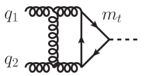
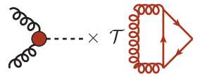
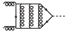
Such an asymptotic expansion can be performed by the method of “expansion by subgraph”, which is conveniently implemented in the program exp [6, 7]. The procedure is to identify all subgraphs of a given Feynman graph which contain the heavy scale (here, ) and expand them in their small quantities. The remaining propagators form the “co-subgraph” which does not depend on the heavy scale. For the problem at hand, this means that each Feynman graph is reduced to a sum of products of massless graphs and -dependent vacuum graphs, after the expansion in the limit . This procedure is depicted in Fig. 1. For the subgraph identified on the first row, the propagators are expanded as follows:
| (1) |
where the “” represent higher-order terms in the expansion. Within the square brackets, the propagators do not carry external momenta or , nor the loop momentum ; there is only a sum of one-loop vacuum integrals with tensor numerators. Such integrals can be computed by the FORM [8] package MATAD [9], up to three-loop order. For computations which require four-loop vacuum integrals we make use of FIRE [10], which we also use to perform integration-by-parts reduction for the massless co-subgraphs. A more complete description of the computational toolchain is given in the following section.
| Full graph | Subgraph | Co-subgraph Expanded subgraph |
|---|---|---|
 |
 |
 |
 |
 |
2.1 Computational Toolchain
For all computations, we begin by generating the necessary Feynman diagrams with qgraf [11]. From here, the packages q2e and exp [6, 7] are used to convert the diagrams into a compatible notation and to identify the relevant subgraphs and co-subgraphs, as described in Section 2. Code is generated for the expansion to be performed by FORM [8], which also computes the colour factors using the COLOR package [12]. Vacuum graphs up to three loops are computed with the MATAD package [9], and four-loop vacuum graphs as well as the massless integrals of the co-subgraphs are reduced to master integrals using FIRE [10]. For the computation of phase-space integrals described in Section 3.1, we use LiteRed [13, 14] and LIMIT [15].
3 Applications
In the following, we summarize some recent works which have used the LME method described above. This includes an NNLO computation of the double-real and real-virtual corrections to double–Higgs boson production in gluon fusion [16, 17, 18] in Section 3.1, and N3LO computations of the virtual corrections to single–Higgs boson production in gluon fusion [19] in Section 3.2, as well as the decay of a Higgs boson into two photons [20] in Section 3.3.
3.1 NNLO real-radiation corrections to double Higgs boson production
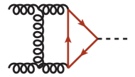
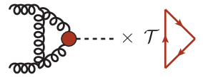
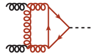
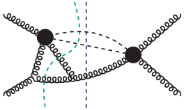
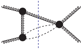
In order to compute real-real and real-virtual corrections we make use of the optical theorem, and compute forward-scattering diagrams which have cuts through the desired final state particles. The real-real corrections correspond to cuts through two Higgs bosons and two additional particles, and the real-virtual corrections to cuts through two Higgs bosons and one additional particle. Examples of such cuts are given in Fig. 2, where the three-particle cuts are shown by blue dashed lines and four-particle cuts by green dashed lines. Some diagrams, such as the first, admit both a three- and four-particle cut. To generate such diagrams an additional step is required to post-process the output of qgraf, which can not itself generate only diagrams containing specified cuts. For this purpose we use the program gen111A. Pak, Unpublished..
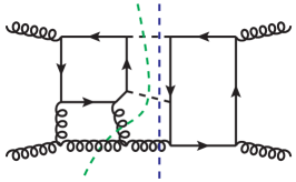
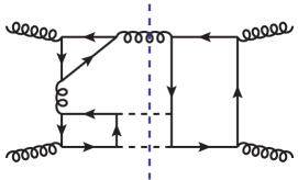
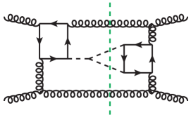
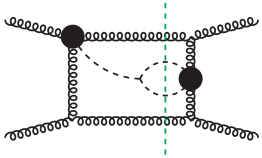
After large- expansion, the diagrams of Fig. 2 yield the phase-space integrals shown in Fig. 3. These integrals are reduced to a basis of master integrals by LiteRed after the partial fractioning of linearly-dependent propagators by LIMIT. The master integrals are computed in an expansion around , which corresponds to the production threshold of the Higgs boson pair. A deep expansion in is obtained efficiently through the use of differential equations, starting from boundary values computed for the leading term in the expansion.
The total cross section at NNLO is given by
| (2) |
where denote the contributing partonic channels, , , , , , including also all additional anti-quark and ghost channels. The collinear counterterms are computed through the convolution of the LO and NLO cross sections with quark or gluon splitting functions. See Section 2.5 of Ref. [18] for a detailed discussion. The virtual corrections have been computed in Ref. [21, 22]. After ultra-violet renormalization, the sum of contributions in Eq. (2) produces a finite result.
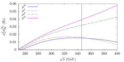
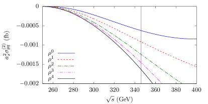
Plots for successive orders of the large- expansion are shown, for the and channels, in Fig. 4. Below the top quark threshold the large- expansion converges well, particularly so close to the production threshold. Compared to the leading expansion term (), which corresponds to the HEFT result (which has been previously computed in Ref. [23]), including the sub-leading terms typically corrects the NNLO contributions by a factor of two.
3.2 N3LO virtual corrections to single Higgs boson production
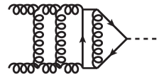
For processes, it is computationally feasible to compute virtual corrections at N3LO, corresponding to four-loop order for loop-induced processes such as single–Higgs boson production in gluon fusion, and Higgs boson decay into two photons (see Section 3.3). Here we compute diagrams such as those shown in Fig. 5. The expansion proceeds in a straightforward manner, as outlined in Section 2. We define the amplitude to be
| (3) |
where are the momenta of the incoming gluons, their colour indices, , and is the Higgs vacuum expectation value. After ultra-violet renormalization, the form factor still contains infra-red poles, however the poles of the rescaled form factor
| (4) |
are predicted to factorize and given in the literature [24]. We thus consider
| (5) |
and find that indeed is independent of and agrees with Ref. [24], and we may study the numerical impact of the N3LO corrections to . At a renormalization scale with an on-shell value of 173 GeV, we find that
| (6) |
where the , and expansion terms have been displayed individually in round brackets. We observe that the sub-leading terms in the large- expansion become increasingly important at higher perturbative orders; at N3LO the and terms correct the term by about 10% and 1%, respectively.
3.3 N3LO corrections to Higgs boson decay into photons
From a computational point of view, the decay process is very similar to discussed above in Section 3.2. The Feynman diagrams which contribute are a subset of those of , i.e., those for which the external gluons (now photons) couple to a quark line rather than internally propagating gluons. The first diagram of Fig. 5 is such an example. We can therefore apply our existing machinery and reduction to master integrals to this process. We define the partial decay width as
| (7) |
and compute in the large- expansion. Unlike the form factor of , is finite after ultra-violet renormalization.
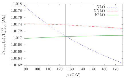
For the top quark mass in the on-shell scheme, Fig. 6 shows the dependence on the renormalization scale of the NLO, NNLO and N3LO corrections, w.r.t. the leading order. At N3LO the curve becomes slightly flatter, but it does not overlap with the NNLO curve.
The N3LO large- result can be combined with the NLO electroweak corrections [25] as well as the NNLO corrections due to bottom and charm quark loops [26],
| (8) |
We find that the N3LO top quark corrections are about the same size as each of the NNLO corrections shown in Eq. (3.3), but come with the opposite sign.
4 Conclusion
In these proceedings, we have discussed the large- expansion and its application to several scattering processes. For processes involving Higgs bosons, the size of the top quark Yukawa coupling means that amplitudes with top quarks running in the loops contribute an important part of the total cross sections. The expansion allows the effect of the top quark mass to be well described below the threshold, and including sub-leading terms typically produces large corrections w.r.t. the leading term alone, which corresponds to the commonly-used HEFT.
Such expansions can be performed in a semi-automated and systematic way, allowing us to study multi-loop amplitudes which can not be computed in an exact manner, either analytically or numerically. As discussed in Section 1, these expansions form the input for various approximation methods which combine information from various kinematic regions, in an attempt to describe multi-loop amplitudes over a wider kinematic range than any one expansion alone.
Acknowledgements
The work of JD was partly supported by the Science and Technology Facilities Council (STFC) under the Consolidated Grant ST/T00102X/1.
References
- [1] G. Aad et al., Search for the process via vector-boson fusion production using proton-proton collisions at TeV with the ATLAS detector, JHEP 07, 108 (2020), 10.1007/JHEP07(2020)108, [Erratum: JHEP 01, 145 (2021), Erratum: JHEP 05, 207 (2021)], 2001.05178.
- [2] A. M. Sirunyan et al., Search for nonresonant Higgs boson pair production in final states with two bottom quarks and two photons in proton-proton collisions at = 13 TeV, JHEP 03, 257 (2021), 10.1007/JHEP03(2021)257, 2011.12373.
- [3] R. Gröber, A. Maier and T. Rauh, Reconstruction of top-quark mass effects in Higgs pair production and other gluon-fusion processes, JHEP 03, 020 (2018), 10.1007/JHEP03(2018)020, 1709.07799.
- [4] J. Davies, R. Gröber, A. Maier, T. Rauh and M. Steinhauser, Top quark mass dependence of the Higgs boson-gluon form factor at three loops, Phys. Rev. D 100(3), 034017 (2019), 10.1103/PhysRevD.100.034017, [Erratum: Phys.Rev.D 102, 059901 (2020)], 1906.00982.
- [5] M. L. Czakon and M. Niggetiedt, Exact quark-mass dependence of the Higgs-gluon form factor at three loops in QCD, JHEP 05, 149 (2020), 10.1007/JHEP05(2020)149, 2001.03008.
- [6] R. Harlander, T. Seidensticker and M. Steinhauser, Complete corrections of Order alpha alpha-s to the decay of the Z boson into bottom quarks, Phys. Lett. B 426, 125 (1998), 10.1016/S0370-2693(98)00220-2, hep-ph/9712228.
- [7] T. Seidensticker, Automatic application of successive asymptotic expansions of Feynman diagrams, In 6th International Workshop on New Computing Techniques in Physics Research: Software Engineering, Artificial Intelligence Neural Nets, Genetic Algorithms, Symbolic Algebra, Automatic Calculation (1999), hep-ph/9905298.
- [8] B. Ruijl, T. Ueda and J. Vermaseren, FORM version 4.2 (2017), 1707.06453.
- [9] M. Steinhauser, MATAD: A Program package for the computation of MAssive TADpoles, Comput. Phys. Commun. 134, 335 (2001), 10.1016/S0010-4655(00)00204-6, hep-ph/0009029.
- [10] A. V. Smirnov and F. S. Chuharev, FIRE6: Feynman Integral REduction with Modular Arithmetic, Comput. Phys. Commun. 247, 106877 (2020), 10.1016/j.cpc.2019.106877, 1901.07808.
- [11] P. Nogueira, Automatic Feynman graph generation, J. Comput. Phys. 105, 279 (1993), 10.1006/jcph.1993.1074.
- [12] T. van Ritbergen, A. N. Schellekens and J. A. M. Vermaseren, Group theory factors for Feynman diagrams, Int. J. Mod. Phys. A 14, 41 (1999), 10.1142/S0217751X99000038, hep-ph/9802376.
- [13] R. N. Lee, Presenting LiteRed: a tool for the Loop InTEgrals REDuction (2012), 1212.2685.
- [14] R. N. Lee, LiteRed 1.4: a powerful tool for reduction of multiloop integrals, J. Phys. Conf. Ser. 523, 012059 (2014), 10.1088/1742-6596/523/1/012059, 1310.1145.
- [15] F. Herren, Precision Calculations for Higgs Boson Physics at the LHC - Four-Loop Corrections to Gluon-Fusion Processes and Higgs Boson Pair-Production at NNLO, Ph.D. thesis, KIT, Karlsruhe, 10.5445/IR/1000125521 (2020).
- [16] J. Davies, F. Herren, G. Mishima and M. Steinhauser, NNLO real corrections to in the large- limit, PoS RADCOR2019, 022 (2019), 10.22323/1.375.0022, 1912.01646.
- [17] J. Davies, F. Herren, G. Mishima and M. Steinhauser, Real-virtual corrections to Higgs boson pair production at NNLO: three closed top quark loops, JHEP 05, 157 (2019), 10.1007/JHEP05(2019)157, 1904.11998.
- [18] J. Davies, F. Herren, G. Mishima and M. Steinhauser, Real corrections to Higgs boson pair production at NNLO in the large top quark mass limit (2021), 2110.03697.
- [19] J. Davies, F. Herren and M. Steinhauser, Top Quark Mass Effects in Higgs Boson Production at Four-Loop Order: Virtual Corrections, Phys. Rev. Lett. 124(11), 112002 (2020), 10.1103/PhysRevLett.124.112002, 1911.10214.
- [20] J. Davies and F. Herren, Higgs boson decay into photons at four loops, Phys. Rev. D 104(5), 053010 (2021), 10.1103/PhysRevD.104.053010, 2104.12780.
- [21] J. Grigo, J. Hoff and M. Steinhauser, Higgs boson pair production: top quark mass effects at NLO and NNLO, Nucl. Phys. B 900, 412 (2015), 10.1016/j.nuclphysb.2015.09.012, 1508.00909.
- [22] J. Davies and M. Steinhauser, Three-loop form factors for Higgs boson pair production in the large top mass limit, JHEP 10, 166 (2019), 10.1007/JHEP10(2019)166, 1909.01361.
- [23] D. de Florian and J. Mazzitelli, Higgs Boson Pair Production at Next-to-Next-to-Leading Order in QCD, Phys. Rev. Lett. 111, 201801 (2013), 10.1103/PhysRevLett.111.201801, 1309.6594.
- [24] T. Gehrmann, E. W. N. Glover, T. Huber, N. Ikizlerli and C. Studerus, Calculation of the quark and gluon form factors to three loops in QCD, JHEP 06, 094 (2010), 10.1007/JHEP06(2010)094, 1004.3653.
- [25] S. Actis, G. Passarino, C. Sturm and S. Uccirati, NNLO Computational Techniques: The Cases H — gamma gamma and H — g g, Nucl. Phys. B 811, 182 (2009), 10.1016/j.nuclphysb.2008.11.024, 0809.3667.
- [26] M. Niggetiedt, Exact quark-mass dependence of the Higgs-photon form factor at three loops in QCD, JHEP 04, 196 (2021), 10.1007/JHEP04(2021)196, 2009.10556.