P3H-19-030 TTP19-028
Three-loop form factors for Higgs boson pair production in the large top mass limit

Abstract

We consider the virtual corrections to Higgs boson pair production at next-to-next-to-leading order, in the large top quark mass limit. We compute five expansion terms for the box-type form factors and eight expansion terms for the triangle form factor, which serve as useful input for the construction of approximations. We present analytic results for the form factors in the soft-virtual approximation.

From a technical point of view the calculation is quite challenging since huge intermediate expressions are produced. We describe our methods and optimizations to overcome these difficulties, which might be useful for other calculations.

1 Introduction

The simultaneous production of two Higgs bosons is a promising process to obtain information about the self-coupling of the Higgs boson and thus the structure of the scalar potential. Although it is experimentally very challenging it is expected that this process can be observed after the high-luminosity upgrade of the LHC.

On the theoretical side there has been quite some effort to obtain precise predictions for differential and total cross sections for Higgs boson pair production. In analogy to single Higgs production the numerically most important contribution is provided by gluon fusion, followed by vector boson fusion, associated production with top quarks and the Higgs-strahlung process (see, e.g., Ref. [1]).

Exact leading order (LO) results for $gg\to HH$ have been available for more than thirty years [2, 3]. Next-to-leading order (NLO) corrections have been computed numerically much more recently, and are available from two independent groups [4, 5, 6]. Note that the numerical evaluations are quite expensive. For this reason it is important to have approximations at hand, which are valid in certain regions of the phase space. Among them are large top quark mass expansions [7, 8, 9] which are available up to order $1/m_{t}^{12}$ [8]. Furthermore, in Ref. [10] an expansion around small transverse momentum has been performed and results in the high-energy region are available from [11, 12]. They have been combined in Ref. [13] with the exact calculation from [4, 5] to provide a precise grid for the NLO virtual corrections [14]. In Ref. [15] exact results for the real radiation contribution have been combined with the effective-theory virtual corrections. Interesting approximations for $gg\to HH$ at NLO have been constructed in Ref. [16] where expansion terms from various regions have been combined with the help of a conformal mapping and Padé approximation. The same method has been been applied in Ref. [17] (using the triangle form factor results of this paper) to the Higgs-gluon form factor, an important ingredient of single-Higgs boson production, in order to reconstruct the full quark mass dependence.

At NNLO exact results are currently out of range, which makes it even more important to obtain approximations, if possible from various kinematic regions. Within the effective theory, where the top quark mass is assumed to be infinitely heavy, NNLO corrections have been computed in Refs. [19, 20, 8]. Power-suppressed terms have been obtained in Ref. [21], where the soft-virtual approximation was constructed. Real corrections which originate from three closed top quark loops have been computed in Ref. [22]. In Ref. [23] approximate NNLO expressions are constructed on the basis of the exact NLO results [5] and further NNLO building blocks which are also available for finite top quark mass. Other NNLO contributions, such as the three-loop virtual corrections, are taken in the infinite top quark mass limit. The results of this paper provide additional $1/m_{t}^{2}$ corrections to the three-loop $gg\to HH$ amplitude which could improve the approximations of Ref. [23].

The resummation of threshold-enhanced logarithms to next-to-next-to-leading logarithmic (NNLL) accuracy has been performed in Refs. [24, 25] and differential distributions up to NNLO for various observables were computed in Ref. [26] in the heavy-top limit. More recently, finite top quark mass effects have also been included [27].

At N³LO first results are available in the limit of infinitely heavy top quarks. In Ref. [28] massless two-loop box contributions have been computed and four-loop corrections to the effective coupling of two Higgs bosons and two, three or four gluons became available from [29, 30].

In this work we consider NNLO virtual corrections to $gg\to HH$ and compute the three relevant form factors for a large top quark mass. We evaluate five expansion terms for the box-type form factors and eight expansion terms for the triangle form factor, i.e., up to order $1/m_{t}^{8}$ and $1/m_{t}^{14}$, respectively. The results for the two box-type form factors are new. The results for the triangle form factor have been obtained in Ref. [31, 32] up to order $1/m_{t}^{8}$, the higher-order expansion terms presented here are new. In a previous work [21] expansion terms up to $1/m_{t}^{4}$ were computed for the (differential) cross section, but not for the form factors. Our results constitute important input for the construction of approximations. For example, it is possible to extend the consideration of Ref. [16] to NNLO. Furthermore, as already mentioned above, it might be possible to improve the approximations of Ref. [23].

The remainder of the paper is organized as follows: in the next section we introduce our notation and define the form factors. We provide technical details in Section 3, and mention several optimizations which were crucial to be able to perform the calculations. Ultraviolet renormalization and infrared subtraction are discussed in Section 4 and both analytical and numerical results are shown in Section 5. We conclude in Section 6.

2 Setup

The amplitude for the process $g(q_{1})g(q_{2})\to H(q_{3})H(q_{4})$ is conveniently decomposed into three form factors. In the following we outline their precise definition. We start with the amplitude which is given by

$${\cal M}^{ab} = \varepsilon_{1,\mu}\varepsilon_{2,\nu}{\cal M}^{\mu\nu,ab}\,\,=\,\,\varepsilon_{1,\mu}\varepsilon_{2,\nu}\delta^{ab}\left({\cal M}_{1}A_{1}^{\mu\nu}+{\cal M}_{2}A_{2}^{\mu\nu}\right)\,,$$ (1)

where $a$ and $b$ are adjoint colour indices and the two Lorentz structures are given by

$$A_{1}^{\mu\nu} = g^{\mu\nu}-{\frac{1}{q_{12}}q_{1}^{\nu}q_{2}^{\mu}}\,,$$

$$A_{2}^{\mu\nu} = g^{\mu\nu}+\frac{1}{p_{T}^{2}q_{12}}\left(q_{33}q_{1}^{\nu}q_{2}^{\mu}-2q_{23}q_{1}^{\nu}q_{3}^{\mu}-2q_{13}q_{3}^{\nu}q_{2}^{\mu}+2q_{12}q_{3}^{\mu}q_{3}^{\nu}\right)\,,$$ (2)

with

$$q_{ij} = q_{i}\cdot q_{j}\,,\qquad p_{T}^{\>2}\>\>\>=\>\>\>\frac{2q_{13}q_{23}}{q_{12}}-q_{33}\,.$$ (3)

${\cal M}_{1}$ and ${\cal M}_{2}$ can be projected from ${\cal M}^{\mu\nu}$ using the projectors

$$P_{1,\mu\nu} = -\,q_{1,\nu}q_{2,\mu}\Bigg{(}\frac{1}{q_{12}}\frac{1-\epsilon}{2-4\epsilon}-\frac{q_{33}}{q_{12}p_{T}^{\>2}}\frac{\epsilon}{2-4\epsilon}\Bigg{)}+\,q_{1,\nu}q_{3,\mu}\Bigg{(}-\frac{2q_{23}}{q_{12}p_{T}^{2}}\frac{\epsilon}{2-4\epsilon}\Bigg{)}$$

$$+\,q_{2,\mu}q_{3,\nu}\Bigg{(}-\frac{2q_{13}}{q_{12}p_{T}^{2}}\frac{\epsilon}{2-4\epsilon}\Bigg{)}-\,q_{3,\mu}q_{3,\nu}\Bigg{(}-\frac{2}{p_{T}^{2}}\frac{\epsilon}{2-4\epsilon}\Bigg{)}+\,g_{\mu\nu}q_{12}\Bigg{(}\frac{1}{q_{12}}\frac{1}{2-4\epsilon}\Bigg{)}\,,$$

$$P_{2,\mu\nu} = q_{1,\nu}q_{2,\mu}\Bigg{(}\frac{q_{33}}{q_{12}p_{T}^{2}}\frac{1-\epsilon}{2-4\epsilon}-\frac{1}{q_{12}}\frac{\epsilon}{2-4\epsilon}\Bigg{)}-\,q_{1,\nu}q_{3,\mu}\Bigg{(}\frac{q_{23}}{q_{12}p_{T}^{2}}\frac{1-\epsilon}{1-2\epsilon}\Bigg{)}$$ (4)

$$-\,q_{2,\mu}q_{3,\nu}\Bigg{(}\frac{q_{13}}{q_{12}p_{T}^{2}}\frac{1-\epsilon}{1-2\epsilon}\Bigg{)}+\,q_{3,\mu}q_{3,\nu}\Bigg{(}\frac{1}{p_{T}^{2}}\frac{1-\epsilon}{1-2\epsilon}\Bigg{)}+\,g_{\mu\nu}q_{12}\Bigg{(}\frac{1}{q_{12}}\frac{1}{2-4\epsilon}\Bigg{)}\,,$$

where $\epsilon=(4-d)/2$ is the standard dimensional regularization parameter.

The Feynman diagrams involving the triple-Higgs boson coupling only contribute to $A_{1}^{\mu\nu}$, which is the only structure relevant for single-Higgs production, therefore it is convenient to decompose ${\cal M}_{1}$ and ${\cal M}_{2}$ into “triangle” and “box” form factors

$${\cal M}_{1} = X_{0}\,s\,\left(\frac{3m_{H}^{2}}{s-m_{H}^{2}}F_{\rm tri}+F_{\rm box1}\right)\,,$$

$${\cal M}_{2} = X_{0}\,s\,F_{\rm box2}\,,$$ (5)

with the prefactor

$$X_{0} = \frac{G_{F}}{\sqrt{2}}\frac{\alpha_{s}(\mu)}{2\pi}Tn_{h}\,,$$ (6)

where $T=1/2$ and $n_{h}=1$ have been introduced for convenience. We furthermore define the expansion of the form factors in $\alpha_{s}$ as

$$F_{X} = \sum_{i\geq 0}\left(\frac{\alpha_{s}(\mu)}{\pi}\right)^{i}F^{(i)}_{X}\,,$$ (7)

with $X\in\{\mbox{tri},\mbox{box1},\mbox{box2}\}$. Note that $F^{(i)}_{X}$ corresponds to the $(i+1)$-loop result. In our final expressions the strong coupling constant is defined with five active quark flavours, which is an appropriate choice since we consider the top quark mass to be large.

In the course of the calculation it is convenient to introduce the Mandelstam variables

$${s}=(q_{1}+q_{2})^{2}\,,\qquad{t}=(q_{1}+q_{3})^{2}\,,\qquad{u}=(q_{2}+q_{3})^{2}\,,$$ (8)

with

$$q_{1}^{2}=q_{2}^{2}=0\,,\qquad q_{3}^{2}=q_{4}^{2}=m_{H}^{2}\,,\qquad s+t+u=2m_{H}^{2}\,.$$ (9)

It is furthermore convenient to express the final result in terms of the transverse momentum of one of the Higgs bosons which is given in terms of the Mandelstam variables by (equivalent to Eq. (3))

$$p_{T}^{2} = \frac{tu-m_{H}^{4}}{s}\,.$$ (10)

3 Calculation details

We generate the Feynman amplitudes with the help of qgraf [33] and obtain 11, 197 and 5703 diagrams at one, two and three loops. Note that both one-particle irreducible (1PI) and one-particle reducible (1PR) contributions have to be considered. Sample diagrams are shown in Fig. 1 together with the corresponding colour factors expressed in terms of the Casimir invariants of SU$(N_{c})$: $C_{A}=N_{c}$ and $C_{F}=(N_{c}^{2}-1)/(2N_{c})$. Furthermore we have $T=1/2$ and use the labels $n_{l}$ and $n_{h}$ for closed massless and massive fermion loops respectively. For numerical evaluation we set $n_{l}=5$ and $n_{h}=1$. In the following subsections we provide several technical details of the calculation of the form factors.

$Tn_{h}$	$Tn_{h}$	$C_{F}Tn_{h}$	$C_{A}Tn_{h}$
$(Tn_{h})^{2}$	$C_{F}^{2}Tn_{h}$	$C_{A}C_{F}Tn_{h}$	$C_{A}^{2}Tn_{h}$
$C_{F}(Tn_{h})^{2}$ and	$C_{A}(Tn_{h})^{2}$ and	$C_{A}(Tn_{h})^{2}$	$(Tn_{h})^{3}$
$C_{F}T^{2}n_{h}n_{l}$	$C_{A}T^{2}n_{h}n_{l}$

Figure 1: Sample Feynman diagrams contributing to $gg\to HH$. For simplicity we show diagrams with a triple-Higgs boson coupling only at one-loop order. A sample colour factor is shown below each diagram. However, note that in general a diagram contributes to more than one colour structure. Solid, dashed and curly lines denote quarks, Higgs bosons and gluons respectively.

3.1 Asymptotic expansion

The programs q2e and exp [34, 35, 36] have been designed to work hand-in-hand when applying a (possibly nested) asymptotic expansion involving a large external momentum or a large internal mass to an amplitude generated by qgraf [33]. The output of exp is FORM [37] code for each sub-diagram which has to be considered according to the rules of asymptotic expansion (see, e.g., Ref. [38]).

In this case we apply the rules of asymptotic expansion for the limit

$$m_{t}\gg q_{1},q_{2},q_{3}\,,$$ (11)

where $q_{1}^{2}=q_{2}^{2}=0$ are the incoming gluon momenta and $q_{3}^{2}=m_{H}^{2}$. Equation (11) implies that the Feynman amplitudes are expanded in powers of

$$\{q_{3}\cdot q_{3},\>\>q_{1}\cdot q_{2},\>\>q_{1}\cdot q_{3},\>\>q_{2}\cdot q_{3}\}/m_{t}^{2},$$ (12)

possibly multiplied by logarithms of these ratios.

The main purpose of Eq. (11) is the reduction of the number of scales in the loop integrals. Furthermore, the three-loop integrals are factorized into products of lower-loop integrals. In the box diagrams we initially have the scales $s$, $t$, $m_{H}^{2}$ and $m_{t}^{2}$ and in the triangle diagrams $s$ and $m_{t}^{2}$. After asymptotic expansion we find the following products of integrals

Type of integrals for		scales
hard subgraph	$\times$ co-subgraph
3-loop vacuum	—	$m_{t}^{2}$
2-loop vacuum	$\times$ 1-loop massless triangle	$m_{t}^{2}\times s$
two 1-loop vacuum	$\times$ 1-loop massless box	$m_{t}^{2}\times s,t,m_{H}^{2}$
1-loop vacuum	$\times$ 2-loop massless triangle	$m_{t}^{2}\times s$

Note that integrals with more than one scale only have to be considered at one-loop order; the corresponding integral families are well-studied in the literature [39, 40, 41]. In the above table “massless” refers to the propagator masses only. Dependence on the Higgs boson mass is retained. In the one-loop massless box case, degenerate cases also occur for which one of the scales is absent.

In cases in which one has to deal with products of integrals we organize the output of exp in such a way that we perform the vacuum integrals first, since it is simpler to compute vacuum tensor integrals than tensor integrals for families with external momenta. In fact, at one and two loops vacuum tensor integrals with arbitrary rank can be treated. For three-loop vacuum integrals we implement projectors which are discussed in detail in Subsection 3.2. For the remaining massless integrations no tensor integrals have to be solved.

The vacuum integrals are performed with the FORM package MATAD [43] and for the massless integral families we use FIRE [44] to obtain integral tables which express all integrals appearing in the amplitudes in terms of master integrals (see Fig. 7 of Ref. [21] for graphical representations). Analytic expressions for the latter can be found in Refs. [39, 40, 41, 21].

Let us illustrate the procedure described above using two typical Feynman diagrams shown in Fig. 2. We show the three-loop diagrams which have to be expanded in all external momenta, and the corresponding lower-loop co-subgraphs which appear after applying the scale hierarchy of Eq. (11). The blobs represent effective vertices from the expanded hard subgraphs which we do not show explicitly.

Figure 2: Sample three-loop diagrams (left) and the corresponding co-subgraphs (right) which result from the asymptotic expansion according to Eq. (11). The blobs represent effective vertices from the hard subgraphs. They correspond to vacuum integrals.

Note that due to the rules of asymptotic expansion the hard subgraphs have to expanded in all small quantities, which in this case are the external momenta $q_{i}$ but also the loop momenta of the co-subgraphs. This results in a multi-dimensional Taylor expansion which we want to compute up to $5^{\rm th}$ order (i.e. up to order $1/(m_{t}^{2})^{4}$) for the box form factors and up to $8^{\rm th}$ order ($1/(m_{t}^{2})^{7}$) for the triangle form factor. At this point the intermediate expressions can become huge and special measures and optimizations have to be applied in order to obtain the results with the computing resources available. These methods are described in the following subsection.

3.2 Projection

A major bottleneck in the computation of [21] is the calculation of three-loop tensor vacuum integrals. After expansion in $1/m_{t}^{2}$ the intermediate expressions become rather large, which cause these routines to perform very poorly. In order to avoid this issue in this work we project the sub-diagrams which contain a three-loop vacuum integral onto a suitable ansatz, and compute individual terms of this ansatz separately. The intermediate expressions for each term become much smaller, and we no longer have to compute tensor integrals. The diagrams contributing to the triangle form factor have a simpler structure, and thus use a simplified version of the method discussed below. For this reason we are able to compute an additional three terms in the expansion, compared to the depth of the box-type form factors. We elaborate on this at the end of the subsection.

Each diagram can be written in the following way, (see also [45], here we extend the ansatz to account for the additional external momentum),

$$A=\sum_{L=0}^{L_{max}}\>\>\sum_{i+j+k+l+m+n=L}C_{i,j,k,l,m,n}\>(q_{1}^{2})^{i}\>(q_{2}^{2})^{j}\>(q_{3}^{2})^{k}\>(q_{1}\cdot q_{2})^{l}\>(q_{1}\cdot q_{3})^{m}\>(q_{2}\cdot q_{3})^{n}.$$ (13)

where $L_{max}$ depends on the depth of the $1/m_{t}^{2}$ expansion being considered. Since we consider the process $g(q_{1})g(q_{2})\rightarrow H(q_{3})H(q_{4})$ we have that $q_{1}^{2}=q_{2}^{2}=0$; we can therefore set $i=j=0$ in the ansatz here. Associated with the six possible scalar products between the momenta are six derivative operators

$$\square_{a,b}=\frac{\partial}{\partial q_{a\>\mu}}\frac{\partial}{\partial q_{b}^{\>\mu}},$$ (14)

with which one can construct projection operators $P_{i,j,k,l,m,n}$ to project particular coefficients $C_{i,j,k,l,m,n}$ of the ansatz $A$ from the amplitude, i.e.

$$P_{i,j,k,l,m,n}\>A=C_{i,j,k,l,m,n}.$$ (15)

It is understood that after taking the derivatives contained in the projector terms, all remaining external momenta of the diagram are set to zero. The first few projection operators are as follows, where we define the notation $\square_{i,j,k,l,m,n}=\square_{1,1}^{\>\>i}\square_{2,2}^{\>\>j}\square_{3,3}^{\>\>k}\square_{1,2}^{\>\>l}\square_{1,3}^{\>\>m}\square_{2,3}^{\>\>n}$ and as above, $d=4-2\epsilon$,

$$L=1:\hskip 28.45274pt$$

$$P_{0,0,0,0,0,1} =\square_{0,0,0,0,0,1}\>\frac{1}{d},\qquad P_{0,0,0,0,1,0}=\square_{0,0,0,0,1,0}\>\frac{1}{d},$$

$$P_{0,0,0,1,0,0} =\square_{0,0,0,1,0,0}\>\frac{1}{d},\qquad P_{0,0,1,0,0,0}=\square_{0,0,1,0,0,0}\>\frac{1}{2d},$$

$$L=2:\hskip 28.45274pt$$

$$P_{0,0,0,0,0,2} =\square_{0,0,0,0,0,2}\>\frac{1}{2d^{2}+2d-4}+\square_{0,1,1,0,0,0}\>\frac{-1}{2d^{3}+2d^{2}-4d},$$

$$P_{0,0,0,0,1,1} =\square_{0,0,0,0,1,1}\>\frac{1}{d^{2}+d-2}+\square_{0,0,1,1,0,0}\>\frac{-1}{d^{3}+d^{2}-2d},$$

$$\vdots$$

$$P_{0,0,1,1,0,0} =\square_{0,0,0,0,1,1}\>\frac{-1}{d^{3}+d^{2}-2d}+\square_{0,0,1,1,0,0}\>\frac{d+1}{2d^{3}+2d^{2}-4d},$$

$$P_{0,0,2,0,0,0} =\square_{0,0,2,0,0,0}\>\frac{1}{8d^{2}+16d}.$$ (16)

For the $1/m_{t}^{8}$ terms we need such projection operators at $L=6$. This is because the vertex diagrams have mass dimension two which are built from combinations of external momenta as required by gauge invariance. Note that contributions involving $\square_{1,1}$ and $\square_{2,2}$ are needed in the construction of the projection operators even though $i=j=0$ is chosen in Eq. (13).

To compute these projections efficiently, we form linear combinations of the projection operators which involve just a single derivative operator $\square_{i,j,k,l,m,n}$. For example at $L=2$, $\square_{0,0,1,1,0,0}$ is present in $P_{0,0,0,0,1,1}$ and $P_{0,0,1,1,0,0}$. Thus, one obtains contributions to the $\left(q_{1}\cdot q_{3}\right)\left(q_{2}\cdot q_{3}\right)$ and $\left(q_{3}\cdot q_{3}\right)\left(q_{1}\cdot q_{2}\right)$ terms of the expansion ansatz by applying the linear combination

$$\bigg{[}\bigg{(}-\frac{1}{72}-\frac{1}{48}\epsilon-\frac{55}{2592}\epsilon^{2}-\frac{95}{5184}\epsilon^{3}+\mathcal{O}(\epsilon^{4})\bigg{)}\left(q_{1}\cdot q_{3}\right)\left(q_{2}\cdot q_{3}\right)+$$

$$\hphantom{\bigg{[}}\bigg{(}\frac{5}{144}+\frac{11}{288}\epsilon+\frac{167}{5184}\epsilon^{2}+\frac{85}{3456}\epsilon^{3}+\mathcal{O}(\epsilon^{4})\bigg{)}\left(q_{3}\cdot q_{3}\right)\left(q_{1}\cdot q_{2}\right)\bigg{]}\>\square_{0,0,1,1,0,0}$$ (17)

to the amplitude. Here the rational polynomials in $d$ have been expanded.

We compute all necessary derivative operators applied to the diagrams after the expansion in $1/m_{t}^{2}$, before we perform the three-loop vacuum integral procedures. Each derivative operator (that is, each $\square_{i,j,k,l,m,n}$ required) is applied as a separate task and all results are combined at the end. This ensures that intermediate expressions remain a manageable size, and that no derivative operator is computed more than once.

For reasonable performance it is crucial to not repeat the $1/m_{t}^{2}$ expansion of the diagrams for each of the above tasks, since it is a very computationally expensive procedure. The expansion is performed just once; the intermediate result is then split into parts containing particular numbers of each external momentum and stored. The projection tasks can load exactly the part which will yield a non-zero result after taking the derivatives with respect to the external momenta.

The structure of the computation is summarized below. For some aspects we provide a more detailed description in Section 3.3.

1. $1/m_{t}^{2}$ expansion:

   1. Sum all diagrams with the same colour factor to make “super-diagrams”. Many terms are common to multiple diagrams, so summing them reduces the total size of the intermediate expressions. At three loops there are 5703 Feynman diagrams which form nine super-diagrams with the colour factors (considering only three-loop vacuum sub-diagrams),

      $$d_{abc}d^{abc}n_{h}^{2},\quad d_{abc}d^{abc}n_{h}n_{l},\quad C_{A}T^{2}n_{h}^{2},\quad C_{F}T^{2}n_{h}^{2},\quad$$

      $$C_{A}^{2}Tn_{h},\quad C_{A}C_{F}Tn_{h},\quad C_{F}^{2}Tn_{h},\quad C_{A}T^{2}n_{h}n_{l},\quad C_{F}T^{2}n_{h}n_{l}.$$ (18)

      The super-diagrams with colour factors proportional to $d_{abc}d^{abc}$, which arise from Feynman diagrams with two closed fermion loops with three gluon couplings each, are found to vanish after expansion in $1/m_{t}^{2}$ in Step 1. (d) (see below), which is why this colour structure is not listed in Fig. 1. Note that of the eight three-loop colour structures listed in Fig. 1 only $(Tn_{h})^{3}$ has no 1PI three-loop vacuum contribution.

   2. For each super-diagram, multiply by one of the five Lorentz structures of the amplitude projectors (c.f. Eq. (2)),

      $$q_{1,\nu}q_{2,\mu},\quad q_{1,\nu}q_{3,\mu},\quad q_{2,\mu}q_{3,\nu},\quad q_{3,\mu}q_{3,\nu},\quad g_{\mu\nu}q_{12}.$$ (19)

      This produces $5\times 9=45$ projected super-diagrams, to be expanded in $1/m_{t}^{2}$. Apply Feynman rules and perform Dirac algebra. The coefficients of these Lorentz structures (in the round brackets of Eq. (2)) will be included when everything is combined in Step 2. (b).

   3. Use graph symmetries to reduce the number of terms and size of expressions.

   4. Perform the $1/m_{t}^{2}$ expansions. These are heavy computations, for which we use computing nodes with relatively large amounts of memory and processing cores (at least 96GB memory and 12 cores). It is crucial to not duplicate any work here; we make extensive use of the FORM statements Collect (to reduce the number of terms to be processed) and ArgToExtraSymbol (to temporarily reduce the size of the expressions). After expansion, graph symmetries are again used to reduce the number of terms and size of the expressions.

      The five most difficult projected super-diagrams are those with colour factor $C_{A}^{2}Tn_{h}$. To expand to $1/m_{t}^{8}$ these each require a wall time of around 10 days. The total size of the (gzip compressed) stored expressions for the expansions of the 45 projected super-diagrams is 324GB.

2. Projection:

   1. For each of the necessary operators (see Eq. (3.2)), load the relevant part of the expanded super-diagram (for the example of Eq. (3.2), the part containing terms with one $q_{1}$, one $q_{2}$ and two $q_{3}$). All other parts would yield zero after differentiation, so do not need to be loaded.

      The differentiation must be performed inside FORM CFunction arguments to avoid an enormous blow-up of intermediate expression sizes. These tasks are much easier, computationally, than those of the expansion steps. They are run requiring only 8GB of memory and 4 processing cores. To obtain the $1/m_{t}^{\{0,2,4,6,8\}}$ terms of the expansion there are {15, 38, 88, 174, 324} derivatives to compute for each of the 45 projected super-diagrams, yielding {675, 1,710, 3,960, 7,830, 14,580} tasks to be run respectively. These tasks required a total time of approximately 1,600 days to complete; running tasks concurrently on our cluster this corresponds to a wall time of about 1 month.

   2. The results of these operators applied to the diagrams allow one to construct the result in the form of the ansatz Eq. (13). Combining all terms, along with the coefficients of the Lorentz structures of Eq. (2), yields the final result for the form factors ${\cal M}_{1}$ and ${\cal M}_{2}$.

As mentioned above, some simplifications are possible when computing the triangle form factor. It comes only with the Lorentz structures $g_{\mu\nu}$ and $q_{1,\nu}q_{2,\mu}$ (see Eq. (2)), thus in step 1. (b) fewer projected super-diagrams are produced since we can ignore the additional three structures required by the box-type form factors. The ansatz of Eq. (13) can also be simplified; only the index $l$ needs to be non-zero. Thus, fewer derivative operators need to be computed in step 2. (a): for the $1/m_{t}^{\{0,2,4,6,8,10,12,14\}}$ terms of the expansion we must apply just $\{2,2,3,3,4,4,5,5\}$ derivative operators.

3.3 Calculation optimizations

In this Section we outline a few methods by which we were able to optimize the computation, in addition to the projection procedure described above. We note that without such optimizations, computing the expansion to a depth $1/m_{t}^{8}$ (and likely $1/m_{t}^{6}$) for the box-type and $1/m_{t}^{14}$ for the triangle form factors would not have been possible with the computing resources available to us.

3.3.1 Graph Symmetries

In Step 1. (c) and 1. (d) we use graph symmetries to reduce the size of the intermediate expressions. We map the vacuum integrals to a minimal set by using rotation and reflection symmetries, implemented by re-labelling the line momenta of equivalent graphs such that they coincide. Some examples of this procedure are shown in Table 1.

After expansion in $1/m_{t}^{2}$ many integrals appear with higher-power (“dotted”) propagators. One can move the dots around the graph, using the same symmetry relations as described above, to obtain a smaller set of integrals.

Top-level Topology	Graph 1	Graph 2	Relabelling
			$\displaystyle p1\rightarrow\hphantom{-}p2$ $\displaystyle p2\rightarrow-p5$ $\displaystyle p3\rightarrow-p4$ $\displaystyle p4\rightarrow\hphantom{-}p3$ $\displaystyle p6\rightarrow-p1$
			$\displaystyle p1\rightarrow\hphantom{-}p2$ $\displaystyle p2\rightarrow-p5$ $\displaystyle p3\rightarrow-p4$ $\displaystyle p5\rightarrow\hphantom{-}p6$ $\displaystyle p6\rightarrow-p1$

Table 1: Graphs 1 and 2 are derived from the Top-level Topology, with different lines missing. This yields different, but equivalent, graphs. Line momenta are relabelled to make this equivalence manifest; we show the replacements required to map Graph 1 onto Graph 2. The arrows denote the direction of momentum flow.

3.3.2 ArgToExtraSymbol

In step 1. (d), the $1/m_{t}^{2}$ expansions are performed. At this point, the FORM representation of the terms in the expressions looks something like

+ Den(l1,mt) * Den(l1+q1,mt) * ... * Den(l2-q3,mt) * ( many terms )

where the Den functions represent the propagators to be expanded; they are of the form $1/(m_{t}^{2}-(l_{1}+q_{1})^{2})$, for example. The “many terms” inside the brackets are coefficients which do not take part in the expansion. Since there can be many thousand such coefficients, it is crucial to keep them bracketed away during the multi-module expansion routine, to keep the number of terms small and avoid expanding the same product of Den functions many times. One typically achieves this with a construction such as

Bracket Den;
.sort
CFunction f;
Collect f;

which moves the bracketed terms inside the argument of f. While this does indeed keep the number of terms small, it does not (greatly) reduce the size of the expression. If the expression is large enough to require disk-based sorting at the end of each module of the expansion routine, one still has a severe performance bottleneck. We resolve this by additionally making use of the statement ArgToExtraSymbol f; after Collect f;, which replaces the (large) arguments of the fs with unique symbols, whose definitions are stored by FORM. More memory is required to store these definitions, but the resulting reduction in size of the expression involved in disk-based sorting provides a large speed-up of the expansion routine. After expansion is complete the original coefficients may be recovered with the FromPolynomial statement.

Let us remark that the use of ArgToExtraSymbol is also essential to make possible and speed up the calculation of the subdiagrams where two-loop vacuum tensor integrals are needed.

3.3.3 Compression

In step 1. (d) it was stated that the intermediate results of the $1/m_{t}^{2}$ expansions are compressed with gzip and stored, for use in step 2. (a). Since these compressed results occupy 324GB, they cannot easily be stored uncompressed on the storage available to us. In step 2. (a) the tasks can easily retrieve the relevant compressed intermediate result from network storage and decompress it onto the local storage of the node on which they are running, by making use of FORM’s #system preprocessor command:

#system gunzip < /network/intermediate.sav.gz > /local/intermediate.sav
Load /local/intermediate.sav;
...

As well as reducing the capacity required for the storage of the intermediate results, this also provides a large performance improvement by reducing the I/O load of the network and storage hardware when hundreds of tasks are running concurrently.

4 Renormalization and infrared subtraction

4.1 Ultraviolet divergences

The renormalization of the ultraviolet (UV) divergences is straightforward:

• The top quark mass ($m_{t}$) renormalization is needed up to two loops. We first renormalize $m_{t}$ in the $\overline{\rm MS}$ scheme, and then transform $m_{t}$ to the on-shell scheme. Note that higher order $\epsilon$ terms are needed in the corresponding one-loop expression since the NLO (two-loop) amplitude develops $1/\epsilon^{2}$ poles, even after all UV counter-terms are taken into account. Since the LO (one-loop) amplitude is finite the two-loop term in the $\overline{\rm MS}$-on-shell conversion formula is only needed up to ${\cal O}(\epsilon^{0})$.

• The gluon wave function renormalization is also needed up to two loops. Note that, since we work in dimensional regularization, where scaleless integrals are set to zero, only diagrams with virtual top quarks contribute. These two-point functions have to be computed for $q^{2}=0$ which corresponds to on-shell gluons. Note that the gluon wave function renormalization agrees with the decoupling constant of the gluon field needed to relate five- and six-flavour QCD [46].

• The strong coupling constant renormalization up to two loops is performed in full six-flavour theory.

• Finally the decoupling relation for $\alpha_{s}$ is needed up to two loops in order to express $\alpha_{s}^{(6)}$ in terms of $\alpha_{s}^{(5)}$. Similar to the $\overline{\rm MS}$–on-shell mass relation also here the one-loop expression is needed up to order $\epsilon^{2}$.

The final result is expressed in terms of the top quark pole mass, and the five-flavour strong coupling, $\alpha_{s}^{(5)}$. It still contains poles up to order $1/\epsilon^{4}$ which are of infrared nature. They will be treated in the next subsection.

4.2 Subtraction of infrared divergences

For the subtraction of the infrared (IR) poles we follow Ref. [47], see also Refs. [48, 8]. For convenience we provide explicit expressions for the subtraction terms. We apply the IR subtraction at the amplitude level since we want the obtain finite expressions for the form factors.

After UV renormalization we have the following colour factors at one-, two- and three-loop order:

$$Tn_{h}\,,$$

$$Tn_{h}\{C_{F},C_{A},Tn_{h},Tn_{l}\}\,,$$

$$Tn_{h}\{C_{F}^{2},C_{A}C_{F},C_{A}^{2},C_{F}Tn_{l},C_{A}Tn_{l},C_{F}Tn_{h},C_{A}Tn_{h},T^{2}n_{l}^{2},T^{2}n_{h}n_{l},T^{2}n_{h}^{2}\}.$$ (20)

In the following discussion we omit the overall factor $Tn_{h}$ which is contained in the quantity $X_{0}$, see Eq. (6). Note that the structures $T^{2}n_{h}n_{l}$, $T^{3}n_{h}n_{l}^{2}$ and $T^{3}n_{h}^{2}n_{l}$ are not present in the two- and three-loop diagrams (cf. Fig. 1) but only arise from UV counter-terms and IR subtraction (see below).

After UV renormalization, at two-loop order the colour factors $\{C_{A},Tn_{l}\}$ come with $1/\epsilon$ poles and $C_{A}$ also has a $1/\epsilon^{2}$ pole. At three-loop order, highest-order pole appearing with each colour factor is summarized in the following table,

Leading Pole	Colour Factors
$1/\epsilon^{4}$	$C_{A}^{2}$
$1/\epsilon^{3}$	$C_{A}Tn_{l}$
$1/\epsilon^{2}$	$C_{A}C_{F}$, $C_{A}Tn_{h}$, $T^{2}n_{l}^{2}$
$1/\epsilon$	$C_{F}Tn_{l}$, $T^{2}n_{h}n_{l}$
$1$	$C_{F}^{2}$, $C_{F}Tn_{h}$, $T^{2}n_{h}^{2}$

We have checked that all these poles cancel after applying the following IR subtraction procedure: finite form factors, $F^{\rm fin}_{X}$, at NLO and NNLO are obtained via

$$F^{(1),\rm fin}_{X} = F^{(1)}_{X}-\frac{1}{2}I^{(1)}_{g}F^{(0)}_{X}\,,$$

$$F^{(2),\rm fin}_{X} = F^{(2)}_{X}-\frac{1}{2}I^{(1)}_{g}F^{(1)}_{X}-\frac{1}{4}I^{(2)}_{g}F^{(0)}_{X}\,,$$ (21)

where, as in Eq. (7), $X\in\{\mbox{tri},\mbox{box1},\mbox{box2}\}$. The quantities on the r.h.s. of Eq. (21) are UV-renormalized. $I^{(1)}_{g}$ and $I^{(2)}_{g}$ on the r.h.s. of Eq. (21) are given by [47, 48]

$$I^{(1)}_{g} = {}-\left(\frac{\mu^{2}}{-s-i\delta}\right)^{\epsilon}\frac{e^{\epsilon\gamma_{E}}}{\Gamma(1-\epsilon)}\frac{1}{\epsilon^{2}}\Big{[}C_{A}+2\epsilon\beta_{0}\Big{]}\,,$$ (22)

$$I^{(2)}_{g} = {}-\left(\frac{\mu^{2}}{-s-i\delta}\right)^{2\epsilon}\left(\frac{e^{\epsilon\gamma_{E}}}{\Gamma(1-\epsilon)}\right)^{2}\frac{1}{\epsilon^{4}}\Big{[}\frac{1}{2}(C_{A}+2\epsilon\beta_{0})^{2}\Big{]}$$ (23)

$${}+\left(\frac{\mu^{2}}{-s-i\delta}\right)^{\epsilon}\frac{e^{\epsilon\gamma_{E}}}{\Gamma(1-\epsilon)}\frac{1}{\epsilon^{3}}\Big{[}2(C_{A}+2\epsilon\beta_{0})\beta_{0}\Big{]}$$

$${}-\left(\frac{\mu^{2}}{-s-i\delta}\right)^{2\epsilon}\frac{e^{\epsilon\gamma_{E}}}{\Gamma(1-\epsilon)}\bigg{\{}\frac{1}{\epsilon^{3}}\Big{[}\frac{1}{2}(C_{A}+4\epsilon\beta_{0})\beta_{0}\Big{]}$$

$$\hskip 56.9055pt-\frac{1}{\epsilon^{2}}\Big{[}\frac{(3\pi^{2}-67)C_{A}+10n_{l}}{72}(C_{A}+4\epsilon\beta_{0})\Big{]}-\frac{1}{\epsilon}\Big{[}\frac{1}{2}H_{g}\Big{]}\bigg{\}}\,,$$

with

$$\beta_{0} = \frac{1}{4}\left(\frac{11}{3}C_{A}-\frac{4}{3}Tn_{l}\right)\,,$$

$$H_{g} = C_{A}^{2}\left(\frac{\zeta_{3}}{2}+\frac{5}{12}+\frac{11\pi^{2}}{144}\right)+C_{A}n_{l}\left(\frac{29}{27}+\frac{\pi^{2}}{72}\right)+\frac{1}{2}C_{F}n_{l}+\frac{5}{27}n_{l}^{2}\,.$$ (24)

5 Results

In the following we discuss the results for the finite form factors constructed according to the prescription of the previous section. Note that the one-loop form factors have no dependence on the renormalization scale $\mu$. At two and three loops the coefficients of the $\log(\mu)$ terms depend on the choice of the IR subtraction terms. In our case it is convenient to cast the results for the two- and three-loop form factors in the following form

$$F_{X}^{{\rm fin},(1)} = \tilde{F}_{X}^{(1)}+l_{\mu s}\beta_{0}\tilde{F}_{X}^{(0)}\,,$$

$$F_{X}^{{\rm fin},(2)} = \tilde{F}_{X}^{(2)}+l_{\mu s}\left(\beta_{1}\tilde{F}_{X}^{(0)}+2\beta_{0}\tilde{F}_{X}^{(1)}\right)+\beta_{0}^{2}l_{\mu s}^{2}\tilde{F}_{X}^{(0)}\,,$$ (25)

where $\tilde{F}^{(i)}_{X}=F^{{\rm fin},(i)}_{X}(\mu^{2}=-s)$ with $\beta_{0}$ as defined in Eq. (4.2) and

$$\beta_{1} = \frac{1}{16}\left(\frac{34}{3}C_{A}^{2}-\frac{20}{3}C_{A}Tn_{l}-4C_{F}Tn_{l}\right)\,,$$

$$l_{\mu s} = \log\left(\frac{\mu^{2}}{-s-i\delta}\right)\,.$$ (26)

The one- and two-loop results are expanded up to order $1/m_{t}^{14}$, the three-loop expressions up to $1/m_{t}^{8}$ (box) and $1/m_{t}^{14}$ (triangle).

For illustration we show the analytic result for the leading term ($m_{t}^{0}$) of the three-loop for factors. The corresponding one- and two-loop results can be found in Ref. [12] and the triangle form factor up to $1/m_{t}^{12}$ with numerical values for the colour factors can be found in Ref. [17]. Our results read

$$\tilde{F}^{(2)}_{\rm tri} = {}C_{F}^{2}\Bigg{[}\frac{9}{8}\Bigg{]}+C_{A}C_{F}\Bigg{[}\frac{11L_{m_{t}^{2}s}}{12}-\frac{25}{9}\Bigg{]}$$ (27)

$$\mbox{}+C_{A}^{2}\Bigg{[}-\frac{7L_{m_{t}^{2}s}}{12}-\frac{253\zeta(3)}{216}+\frac{\pi^{4}}{864}+\frac{19\pi^{2}}{108}+\frac{19777}{3888}\Bigg{]}$$

$$\mbox{}+C_{F}n_{l}\Bigg{[}-\frac{L_{m_{t}^{2}s}}{3}+\frac{2\zeta(3)}{3}-\frac{41}{36}\Bigg{]}+C_{A}n_{l}\Bigg{[}-\frac{49\zeta(3)}{108}-\frac{2255}{1944}-\frac{47\pi^{2}}{1296}\Bigg{]}$$

$$\mbox{}+C_{F}n_{h}\Bigg{[}-\frac{1}{18}\Bigg{]}+C_{A}n_{h}\Bigg{[}-\frac{5}{144}\Bigg{]}+n_{l}^{2}\Bigg{[}\frac{\pi^{2}}{648}\Bigg{]}\,,$$

$$\tilde{F}^{(2)}_{\rm box1} = -\tilde{F}^{(2)}_{\rm tri}+C_{A}C_{F}\Bigg{[}\frac{11}{6}\Bigg{]}+C_{A}^{2}\Bigg{[}-\frac{7}{6}\Bigg{]}+C_{F}n_{l}\Bigg{[}-\frac{2}{3}\Bigg{]}+C_{F}n_{h}\Bigg{[}-1\Bigg{]}$$ (28)

$$\mbox{}+C_{A}n_{h}\Bigg{[}-\frac{2m_{H}^{4}\mbox{Li}_{2}\left(1-\frac{m_{H}^{4}}{tu}\right)}{9s^{2}}-\frac{4m_{H}^{4}\mbox{Li}_{2}\left(\frac{m_{H}^{2}}{t}\right)}{9s^{2}}-\frac{4m_{H}^{4}\mbox{Li}_{2}\left(\frac{m_{H}^{2}}{u}\right)}{9s^{2}}$$

$$\mbox{}-\frac{1}{9}\mbox{Li}_{2}\left(1-\frac{m_{H}^{4}}{tu}\right)-\frac{2}{9}\mbox{Li}_{2}\left(\frac{m_{H}^{2}}{t}\right)-\frac{2}{9}\mbox{Li}_{2}\left(\frac{m_{H}^{2}}{u}\right)-\frac{4L_{m_{H}^{2}t}m_{H}^{4}\log\left(1-\frac{m_{H}^{2}}{t}\right)}{9s^{2}}$$

$$\mbox{}-\frac{2}{9}L_{m_{H}^{2}t}\log\left(1-\frac{m_{H}^{2}}{t}\right)-\frac{4L_{m_{H}^{2}u}m_{H}^{4}\log\left(1-\frac{m_{H}^{2}}{u}\right)}{9s^{2}}-\frac{2}{9}L_{m_{H}^{2}u}\log\left(1-\frac{m_{H}^{2}}{u}\right)$$

$$\mbox{}+\frac{11L_{st}}{54}+\frac{11L_{su}}{54}+\frac{m_{H}^{4}\log^{2}\left(\frac{t}{u}\right)}{9s^{2}}+\frac{4\pi^{2}m_{H}^{4}}{27s^{2}}+\frac{2m_{H}^{2}}{9s}+\frac{1}{18}\log^{2}\left(\frac{t}{u}\right)+\frac{2\pi^{2}}{27}$$

$$\mbox{}+\frac{193}{81}\Bigg{]}+n_{l}n_{h}\Bigg{[}-\frac{L_{st}}{27}-\frac{L_{su}}{27}-\frac{10}{81}\Bigg{]}\,,$$

where $T=1/2$ has been chosen and the overall factor $n_{h}$ is contained in Eq. (6). Furthermore, we have introduced

$$L_{st} = \log\left(-\frac{s}{t}\right)-i\pi\,,$$

$$L_{su} = \log\left(-\frac{s}{u}\right)-i\pi\,,$$

$$L_{m_{t}^{2}s} = \log\left(\frac{m_{t}^{2}}{s}\right)+i\pi\,,$$

$$L_{m_{H}^{2}t} = \log\left(-\frac{m_{H}^{2}}{t}\right)-i\pi\,,$$

$$L_{m_{H}^{2}u} = \log\left(-\frac{m_{H}^{2}}{u}\right)-i\pi\,.$$ (29)

We refrain from showing explicit results for $\tilde{F}^{(2)}_{\rm box2}$ which has a similar structure to $\tilde{F}^{(2)}_{\rm box1}$. Note that for most colour structures $\tilde{F}^{(2)}_{\rm box2}$ starts at order $1/m_{t}^{2}$ except for the three colour structures $C_{F}n_{h}$, $C_{A}n_{h}$ and $n_{l}n_{h}$ which arise from (1PR and 1PI) diagrams with two closed top quark loops. The analytic results for the one- and two-loop box and triangle form factors expanded up to $1/m_{t}^{12}$ and $1/m_{t}^{14}$ respectively, the three-loop box form factors $\tilde{F}^{(2)}_{\rm box1}$ and $\tilde{F}^{(2)}_{\rm box2}$ expanded up to $1/m_{t}^{8}$, and the three-loop triangle form factor $\tilde{F}^{(2)}_{\rm tri}$ expanded up to up to $1/m_{t}^{14}$ can be found in the supplementary file of this paper [49].

Note that at two-loop order the 1PI (colour structures $C_{A}Tn_{h}$ and $C_{F}Tn_{h}$) and 1PR ($(Tn_{h})^{2}$) contributions are separately finite. At three-loop order this is not the case and the whole contribution has to be considered in order to arrive at finite form factors, see also discussion in Refs. [30, 8].

Let us now briefly discuss the numerical impact of our calculation. For the numerical evaluation we use $m_{t}=173$ GeV and $m_{H}=125$ GeV and for the transverse momentum we introduce the parameter

$$r_{p_{T}} = \frac{p_{T}^{2}}{s}\,,$$ (30)

with $r_{p_{T}}=0.01$ as default value. Furthermore we choose for the parameters introduced for closed fermion loops $n_{l}=5$ and $n_{h}=1$.

Figure 3: Real parts of one- and two-loop form factors as a function of $\sqrt{s}$ for $r_{p_{T}}=0.01$.

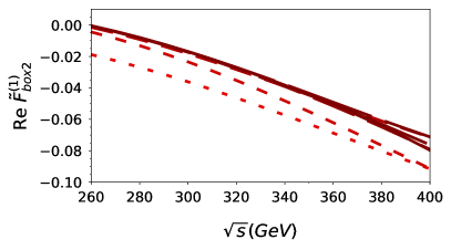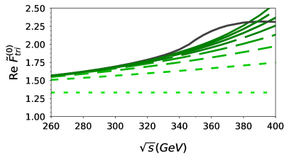
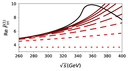
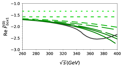
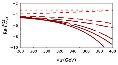
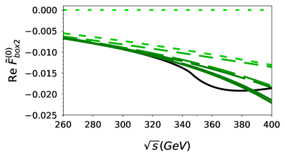
In Fig. 3 we show real parts of the one- and two-loop results for the three form factors as a function of $\sqrt{s}$. We include terms up to order $1/m_{t}^{14}$ for the triangle and order $1/m_{t}^{12}$ for the box form factors. Lines with longer dashes include more expansion terms. Below the threshold, i.e. for $\sqrt{s}\;\hbox to0.0pt{\lower 3.5pt\hbox{$\mathchar 0\relax\sim$}\hss}\raise 1.0pt\hbox{$<$}\;2m_{t}$, one observes a reasonable convergence of the expansion in $1/m_{t}^{2}$ as can be seen by the reduced distance between the dashed curves. In this respect, $F^{(0)}_{\rm box2}$ and $F^{(1)}_{\rm box2}$ are particularly well-behaved; after including the third expansion term the curves lie practically on top of each other. At one-loop order we also find good agreement with the exact results (solid black curves) for $\sqrt{s}\;\hbox to0.0pt{\lower 3.5pt\hbox{$\mathchar 0\relax\sim$}\hss}\raise 1.0pt\hbox{$<$}\;320$ GeV. For the two-loop triangle form factor we find agreement with the exact expression (see Refs. [50, 51, 52] for analytic expressions) for $\sqrt{s}\;\hbox to0.0pt{\lower 3.5pt\hbox{$\mathchar 0\relax\sim$}\hss}\raise 1.0pt\hbox{$<$}\;300$ GeV.

Note that the form factors also develop imaginary parts which originate from contributions with massless cuts, see co-subgraphs in Fig. 2. They are contained in our analytic expressions [49], but are not plotted here.

Figure 4: Real parts of three-loop form factors as a function of $\sqrt{s}$ for $r_{p_{T}}=0.1$.

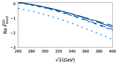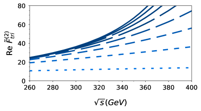
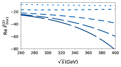
A similar behaviour to the one- and two-loop cases is observed at three-loop order as can be seen in Fig. 4. We want to stress that qualitatively the two- and three-loop corrections show a very similar behaviour. Since the two-loop terms have proven to provide useful and important input into the Padé procedure [16], which can be used to obtain approximations valid in the whole $\sqrt{s}$ region, we expect that the three-loop terms are of similar importance.

For some applications it is advantageous to rescale the higher order corrections by the exact leading order contributions using

$$\frac{\tilde{F}_{X}^{(n),\rm exp}}{\tilde{F}_{X}^{(0),\rm exp}}\tilde{F}_{X}^{(0),\rm exact}\,,$$ (31)

where $\tilde{F}_{X}^{(n),\rm exp}$ and $\tilde{F}_{X}^{(0),\rm exp}$ are expanded up to the same order in $1/m_{t}$. We refrain from showing the corresponding results but simply want to mention that the differences between the $\tilde{F}_{X}^{(n),\rm exp}$ and the rescaled expression (31) become smaller with increasing order in $1/m_{t}$. In fact the curves which correspond to the deepest expansions are very close to each other.

6 Conclusions

We compute three-loop corrections to the process $gg\to HH$ in the large-$m_{t}$ limit and provide results for five expansion terms (up to order $1/m_{t}^{8}$) for the two box-type form factors and for eight expansion terms (up to order $1/m_{t}^{14}$) for the triangle form factor. As compared to previous work [21] we have computed two more expansion terms, which required significant reorganization and optimization of the calculations since huge expressions are obtained at various intermediate stages. We discuss these modifications in Section 3. Furthermore in Ref. [21] only partonic cross sections, rather than individual form factors, are available.

The analytic results for the form factors, which are provided in a computer-readable form in supplementary material [49], are useful input for the construction of approximations for $gg\to HH$ at NNLO, both for total cross sections and differential distributions. This concerns both the construction of Padé approximants along the lines of [16] (indeed these new results for the triangle form factor have already been used in [17]) but also approximation procedures which have been employed in Ref. [23].

Appendix A README for the supplementary material

In this Appendix we provide a brief explanation of the notation used in the ancillary file to this paper [49].

Our final results for the form factors are contained in the file resFF.m where the following notation has been used:

F1tri	F2tri	F3tri	F1box1	F2box1	F3box1	F1box2	F2box2	F3box2
$\tilde{F}^{(0)}_{\rm tri}$	$\tilde{F}^{(1)}_{\rm tri}$	$\tilde{F}^{(2)}_{\rm tri}$	$\tilde{F}^{(0)}_{\rm box1}$	$\tilde{F}^{(1)}_{\rm box1}$	$\tilde{F}^{(2)}_{\rm box1}$	$\tilde{F}^{(0)}_{\rm box2}$	$\tilde{F}^{(1)}_{\rm box2}$	$\tilde{F}^{(2)}_{\rm box2}$

The expressions have the same colour factors as in Eq. (20) where $T=1/2$ has been chosen and the overall factor $n_{h}$ has been set to 1. The following variables are used ca, cf, nh, nl, mH2 $=m_{H}^{2}$ mt2$=m_{t}^{2}$, s, t. Furthermore the functions Li2[_] and Log[_] are used with obvious meaning.

References

- [1] J. Baglio, A. Djouadi, R. Gröber, M. M. Mühlleitner, J. Quevillon and M. Spira, JHEP 1304 (2013) 151 [arXiv:1212.5581 [hep-ph]].
- [2] E. W. N. Glover and J. J. van der Bij, Nucl. Phys. B 309 (1988) 282.
- [3] T. Plehn, M. Spira and P. M. Zerwas, Nucl. Phys. B 479 (1996) 46 Erratum: [Nucl. Phys. B 531 (1998) 655] [hep-ph/9603205].
- [4] S. Borowka, N. Greiner, G. Heinrich, S. P. Jones, M. Kerner, J. Schlenk, U. Schubert and T. Zirke, Phys. Rev. Lett. 117 (2016) no.1, 012001 Erratum: [Phys. Rev. Lett. 117 (2016) no.7, 079901] [arXiv:1604.06447 [hep-ph]].
- [5] S. Borowka, N. Greiner, G. Heinrich, S. P. Jones, M. Kerner, J. Schlenk and T. Zirke, JHEP 1610 (2016) 107 [arXiv:1608.04798 [hep-ph]].
- [6] J. Baglio, F. Campanario, S. Glaus, M. Mühlleitner, M. Spira and J. Streicher, Eur. Phys. J. C 79 (2019) no.6, 459 [arXiv:1811.05692 [hep-ph]].
- [7] S. Dawson, S. Dittmaier and M. Spira, Phys. Rev. D 58 (1998) 115012 [hep-ph/9805244].
- [8] J. Grigo, K. Melnikov and M. Steinhauser, Nucl. Phys. B 888 (2014) 17 [arXiv:1408.2422 [hep-ph]].
- [9] G. Degrassi, P. P. Giardino and R. Gröber, Eur. Phys. J. C 76 (2016) no.7, 411 [arXiv:1603.00385 [hep-ph]].
- [10] R. Bonciani, G. Degrassi, P. P. Giardino and R. Gröber, Phys. Rev. Lett. 121 (2018) no.16, 162003 [arXiv:1806.11564 [hep-ph]].
- [11] J. Davies, G. Mishima, M. Steinhauser and D. Wellmann, JHEP 1803 (2018) 048 [arXiv:1801.09696 [hep-ph]].
- [12] J. Davies, G. Mishima, M. Steinhauser and D. Wellmann, JHEP 1901 (2019) 176 [arXiv:1811.05489 [hep-ph]].
- [13] J. Davies, G. Heinrich, S. P. Jones, M. Kerner, G. Mishima, M. Steinhauser and D. Wellmann, arXiv:1907.06408 [hep-ph].
-
[14]
https://github.com/mppmu/hhgrid. - [15] F. Maltoni, E. Vryonidou and M. Zaro, JHEP 1411 (2014) 079 [arXiv:1408.6542 [hep-ph]].
- [16] R. Gröber, A. Maier and T. Rauh, JHEP 1803 (2018) 020 [arXiv:1709.07799 [hep-ph]].
- [17] J. Davies, R. Gröber, A. Maier, T. Rauh and M. Steinhauser, Phys. Rev. D 100 (2019) 034017 [arXiv:1906.00982 [hep-ph]].
- [18] R. V. Harlander, M. Prausa and J. Usovitsch, arXiv:1907.06957 [hep-ph].
- [19] D. de Florian and J. Mazzitelli, Phys. Lett. B 724 (2013) 306 [arXiv:1305.5206 [hep-ph]].
- [20] D. de Florian and J. Mazzitelli, Phys. Rev. Lett. 111 (2013) 201801 [arXiv:1309.6594 [hep-ph]].
- [21] J. Grigo, J. Hoff and M. Steinhauser, Nucl. Phys. B 900 (2015) 412 [arXiv:1508.00909 [hep-ph]].
- [22] J. Davies, F. Herren, G. Mishima and M. Steinhauser, JHEP 1905 (2019) 157 [arXiv:1904.11998 [hep-ph]].
- [23] M. Grazzini, G. Heinrich, S. Jones, S. Kallweit, M. Kerner, J. M. Lindert and J. Mazzitelli, JHEP 1805 (2018) 059 [arXiv:1803.02463 [hep-ph]].
- [24] D. Y. Shao, C. S. Li, H. T. Li and J. Wang, JHEP 1307 (2013) 169 [arXiv:1301.1245 [hep-ph]].
- [25] D. de Florian and J. Mazzitelli, JHEP 1509 (2015) 053 [arXiv:1505.07122 [hep-ph]].
- [26] D. de Florian, M. Grazzini, C. Hanga, S. Kallweit, J. M. Lindert, P. Maierhöfer, J. Mazzitelli and D. Rathlev, JHEP 1609 (2016) 151 [arXiv:1606.09519 [hep-ph]].
- [27] D. De Florian and J. Mazzitelli, JHEP 1808 (2018) 156 [arXiv:1807.03704 [hep-ph]].
- [28] P. Banerjee, S. Borowka, P. K. Dhani, T. Gehrmann and V. Ravindran, JHEP 1811 (2018) 130 [arXiv:1809.05388 [hep-ph]].
- [29] M. Spira, JHEP 1610 (2016) 026 [arXiv:1607.05548 [hep-ph]].
- [30] M. Gerlach, F. Herren and M. Steinhauser, JHEP 1811 (2018) 141 [arXiv:1809.06787 [hep-ph]].
- [31] R. V. Harlander and K. J. Ozeren, Phys. Lett. B 679 (2009) 467 [arXiv:0907.2997 [hep-ph]].
- [32] A. Pak, M. Rogal and M. Steinhauser, Phys. Lett. B 679 (2009) 473 [arXiv:0907.2998 [hep-ph]].
- [33] P. Nogueira, J. Comput. Phys. 105 (1993) 279.
- [34] R. Harlander, T. Seidensticker and M. Steinhauser, Phys. Lett. B 426 (1998) 125 [hep-ph/9712228].
- [35] T. Seidensticker, hep-ph/9905298.
[36]
http://sfb-tr9.ttp.kit.edu/software/html/q2eexp.html. - [37] B. Ruijl, T. Ueda and J. Vermaseren, arXiv:1707.06453 [hep-ph].
- [38] V. A. Smirnov, Springer Tracts Mod. Phys. 250 (2012) 1.
- [39] T. G. Birthwright, E. W. N. Glover and P. Marquard, JHEP 0409 (2004) 042 [hep-ph/0407343].
- [40] R. K. Ellis and G. Zanderighi, JHEP 0802 (2008) 002 [arXiv:0712.1851 [hep-ph]].
- [41] F. Chavez and C. Duhr, JHEP 1211 (2012) 114 [arXiv:1209.2722 [hep-ph]].
- [42] K. G. Chetyrkin, In *Oberammergau 1993, New computing techniques in physics research III* 559-563 [hep-ph/0212040].
- [43] M. Steinhauser, Comput. Phys. Commun. 134 (2001) 335 [hep-ph/0009029].
- [44] A. V. Smirnov, Comput. Phys. Commun. 189 (2015) 182 [arXiv:1408.2372 [hep-ph]].
- [45] J. Fleischer and O. V. Tarasov, Z. Phys. C 64 (1994) 413 [hep-ph/9403230].
- [46] K. G. Chetyrkin, B. A. Kniehl and M. Steinhauser, Nucl. Phys. B 510 (1998) 61 [hep-ph/9708255].
- [47] S. Catani, Phys. Lett. B 427 (1998) 161 [hep-ph/9802439].
- [48] D. de Florian and J. Mazzitelli, JHEP 1212 (2012) 088 [arXiv:1209.0673 [hep-ph]].
[49]
https://www.ttp.kit.edu/preprints/2019/ttp19-028/. - [50] R. Harlander and P. Kant, JHEP 0512 (2005) 015 [hep-ph/0509189].
- [51] C. Anastasiou, S. Beerli, S. Bucherer, A. Daleo and Z. Kunszt, JHEP 0701 (2007) 082 [hep-ph/0611236].
- [52] U. Aglietti, R. Bonciani, G. Degrassi and A. Vicini, JHEP 0701 (2007) 021 [hep-ph/0611266].