TTP19-042, P3H-19-048
NNLO real corrections to $gg\to HH$ in the large-$m_{t}$ limit

Abstract:

In this contribution we consider NNLO real radiation corrections to the total cross section for Higgs boson pair production in gluon fusion. Special emphasis is put on the cross check of the asymptotic expansion in the inverse top quark mass.

1 Introduction

After the discovery of the Higgs boson [1, 2] all parameters and couplings of the Standard Model (SM) are fixed. In particular, the coupling strength for the interaction of three and four Higgs bosons is given by $\lambda=m_{H}^{2}/(2v^{2})\approx 0.13$ where $m_{H}$ is the Higgs boson mass and $v$ is the vacuum expectation value. However, many beyond-the-SM theories implement a different scalar sector. It is thus desirable to obtain independent information about the Higgs boson self coupling from experimental measurements. A promising process in this context is double Higgs boson production.

In the recent years many higher order corrections to Higgs boson pair production have become available, in particular for the numerically most important channel $gg\to HH$. In this proceedings contribution we refrain from providing a detailed listing of all relevant works but refer to a recent review [3] and references cited therein.

The aim of this contribution is to summarize the work [4] and provide further technical details on the extension to the contribution with two closed top quark loops. In particular, we confront the “building-block-approach” with the naive use of asymptotic expansion.

2 Setup

In the following we briefly describe the individual steps which we follow in order to arrive at analytic results for the partonic cross section for $gg\to HH$. We are interested in computing the imaginary part of the forward-scattering amplitude $g(q_{1})g(q_{2})\to g(q_{1})g(q_{2})$ due to cuts involving two Higgs bosons and possibly further light (anti-)quarks or gluons. Note that at LO, NLO and NNLO this leads to three-, four- and five-loop diagrams; all of them have closed top quark loops both left and right of the cut. In fact, we can classify the diagrams according to the number of closed top quark loops which involve at least one coupling to a Higgs boson. The real radiation corrections at NNLO have either two or three, which we denote by $n_{h}^{2}$ and $n_{h}^{3}$ contributions, respectively. Results for the $n_{h}^{3}$ contribution have been published in Ref. [4]. At LO there are only $n_{h}^{2}$ diagrams. $n_{h}^{3}$ contributions appear for the first time at NLO as virtual corrections as can be seen in Fig. 1 (NNLO $n_{h}^{3}$ diagrams are shown in Fig. 2.) The virtual corrections at NNLO also have $n_{h}^{4}$ terms.

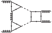
Figure 1: One LO and three NLO sample Feynman diagrams for $gg\to gg$. Solid, dashed and curly lines represent quarks, Higgs bosons and gluons, respectively. The contributions to the Higgs boson pair production cross section are obtained by considering cuts which involve at least two Higgs bosons. The third diagram represents the $n_{h}^{3}$ contribution at NLO.

We generate the amplitudes of the individual Feynman diagrams using qgraf [5]. After specifying the particle content this leads to $16.6\times 10^{6}$ diagrams. However, many of them have no relevant cuts. For example, in many cases the Higgs bosons are generated in the $t$ instead of the $s$ channel. We thus apply additional scripts to select the contributions containing the relevant cuts which significantly reduces the number of diagrams to $0.16\times 10^{6}$; $12,114$ of them contribute to the $n_{h}^{3}$ terms.

Instead of generating five-loop amplitudes (at NNLO) it is possible to interpret the subdiagrams containing the top quark as effective vertices which mediate the coupling of up to two Higgs bosons, up to four gluons and up to one quark-anti-quark pair. One can pre-compute the large-$m_{t}$ expansion of these one- and two-loop tadpole integrals using using MATAD [6] and store the results to disk. Afterwards we generate $g(q_{1})g(q_{2})\to g(q_{1})g(q_{2})$ amplitudes up to three loops using effective vertices in the qgraf input file. In the course of the calculation the effective vertices are replaced by the pre-computed results for the top quark loops. We call this approach the “building-block approach” and provide more details in Section 4.

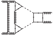
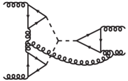
Figure 2: Sample NNLO Feynman diagrams for $ij\to ij$ with $i,j\in\{g,q\}$. Solid, dashed and curly lines represent quarks, Higgs bosons and gluons, respectively. The contributions to the Higgs boson pair production cross section are obtained by considering cuts which involve at least two Higgs bosons. All diagrams are $n_{h}^{3}$ contributions except the second and the third diagram in the first row, which are not included in our final result. They contain a closed top quark loop without a coupling to the Higgs boson.

The modified qgraf output is then processed by q2e and exp [7, 8, 9], which generate FORM [10] code for the amplitudes and map them onto the predefined integral families. We compute the colour factors of the diagrams using color [11].

Next, we must apply partial fraction decompositions to arrive at a unique set of integral families. This is necessary since we consider four-point functions but have only two independent external momenta. In fact, for our kinematic configuration we have 3, 7 and 12 independent kinematic invariants (and thus scalar functions with 3, 7 and 12 indices) at one, two and three loops, respectively. A subsequent reduction, which we perform with the help of LiteRed [12, 13], leads to master integrals which depend on

$$x = \frac{m_{H}^{2}}{s}\,.$$ (1)

In the physical region we have $0<x<1/4$. In the next section we discuss the evaluation of the master integrals for the NNLO $n_{h}^{3}$ term.

3 $n_{h}^{3}$ contribution

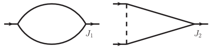
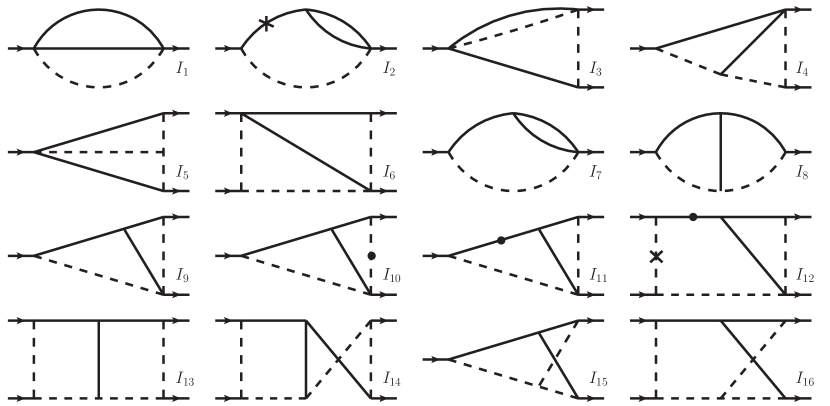
Figure 3: One- (first row) and two-loop master integrals. Solid and dashed lines represent massive and massless propagators. Dots and crosses denote squared and inverse propagators, respectively. It is understood that the momenta $q_{1}$ and $q_{2}$ enter the diagrams on the left and leave them on the right in the upper and lower lines, respectively. For the external momenta we have $q_{1}^{2}=q_{2}^{2}=0$ and $(q_{1}+q_{2})^{2}=s$.

Sample Feynman diagrams which have to be considered for the NNLO $n_{h}^{3}$ contribution are shown in Fig. 2. The virtual corrections have been computed in Refs. [14, 15]. As for the real corrections, each diagram in the second row is a representative of one of the three partonic channels, $gg$, $qg$ and $q\bar{q}$. After applying the steps described in the previous section we can express the $gg\to gg$ amplitude as a linear combination of 2 one-loop and 16 two-loop master integrals which we show in Fig. 3. They depend on $x$ and analytic results are obtained using the method of differential equations [16, 17, 18].

The master integrals shown in Fig. 3 can be transformed into the so-called $\epsilon$ form of the differential equation, which has the particularly simple form

$$\frac{{\rm d}I}{{\rm d}y} = \epsilon\sum_{i}\frac{A_{i}}{y-y_{i}}I\,,$$ (2)

where $I$ is the vector of master integrals and $A_{i}$ are square matrices with constant (i.e., independent of $y$ and $\epsilon$) matrix elements. Due to the fact that in Eq. (2) $\epsilon$ factorizes and the $y$ dependence only occurs in form of simple poles it is straightforward to construct solutions of $I$ in terms of iterated integrals (Goncharov polylogarithms [19]) provided we have boundary conditions for $I$ for some value of $y$. We have chosen the so-called soft limit which corresponds to

$$\delta\equiv\sqrt{1-4x}\to 0\,,\quad\mbox{i.e.}\quad x\to 1/4\quad\mbox{and}\quad y\to-1.$$ (3)

In this contribution we refrain from discussing details about the computation of the boundary values; they can be found in Ref. [4].

In order to arrive at Eq. (2) one has to apply ideas developed in Refs. [20, 21] which help to transform the original system of differential equations into Eq. (2). In practice, we use the program Epsilon [22] which is based on the algorithm provided in Ref. [21]. In an intermediate step we observe poles in $x$ at the positions $x=\{0,1/4,1,r_{1}=\exp(i\pi/3),r_{2}=\exp(-i\pi/3),-1/3\}$ A closer inspection of the corresponding matrices suggests the variable transformation

$$y = \frac{\sqrt{1-4x}-1}{\sqrt{1-4x}+1},~{}-1<y<0\,,$$ (4)

which leads to an $\epsilon$ form for the first 14 (out of 16) master integrals, as discussed in Ref. [4]. The explicit construction of an $\epsilon$ form for the remaining two master integrals can be avoided since at most their leading $\epsilon$ term enters the physical result.

As an alternative to the exact solution of Eq. (2) in terms of generalized logarithms one can use the differential equation together with the boundary conditions to construct many terms of an expansion in $\delta$. We managed to obtain, without much difficulty, more than 500 expansion terms; these are more than sufficient for all practical purposes.

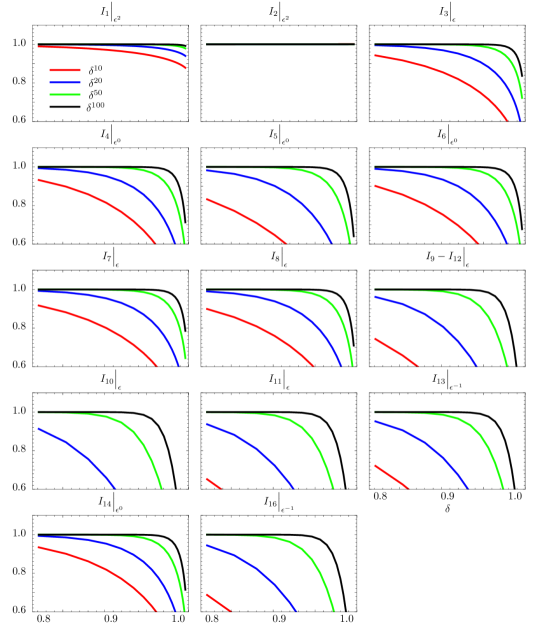
Figure 4: Two-loop master integrals of Fig. 3 as a function of $\delta$. We show the highest $\epsilon$ term which enters the finite result of the physical amplitude. The curves include expansions in $\delta$ up to order $\delta^{10}$, $\delta^{20}$, $\delta^{50}$ and $\delta^{100}$ normalized to the exact result. Note that $I_{15}$ is finite and enters the amplitude with a prefactor proportional to $\epsilon$. Note that in the case of $I_{2}$ the higher order $\delta$ terms rapidly become quite small which is the reason for the good convergence.

In Fig. 4 we show, for each master integral, the highest $\epsilon$ term needed for the physical amplitude. We normalize the different expansions to the exact result and plot the ratio as a function of $\delta$. Note that $I_{15}$ does not contribute to the amplitude. However, it is needed for the computation of $I_{16}$ since $I_{15}$ is present in one of its subsectors. In all cases, one observes good agreement between the exact result and the expansion (including terms to $\delta^{50}$) in the region $\delta\leq 0.9$. We note that $\delta=0.9$ corresponds to $\sqrt{s}\approx 800$ GeV. This has to be compared with the validity range of the large-$m_{t}$ expansion (see below) which is for $\sqrt{s}\;\hbox to0.0pt{\lower 3.5pt\hbox{$\mathchar 0\relax\sim$}\hss}\raise 1.0pt\hbox{$<$}\;2m_{t}\approx 350$ GeV.

For illustration we show in Fig. 5 the partonic cross section for the NNLO $n_{h}^{3}$ contribution $gg$ channel as a function of $\sqrt{s}$ [4], where expansion terms up to ${\cal O}(\delta^{35})$ are included. This expansion depth is sufficient since we only plot results up to $\sqrt{s}=500$ GeV. We observe a reasonable convergence below the top threshold. Above $\sqrt{s}\approx 350$ GeV the curves diverge which is expected since the assumed hierarchy $m_{t}^{2}\ll s$ does not hold in this region. Although the region of convergence is small the power corrections provide important input for the construction of an approximate NNLO result. For example, in Ref. [23] NLO virtual corrections have been considered and the inclusion of higher order $1/m_{t}$ terms significantly stabilizes the Padé results obtained by combining information from large-$m_{t}$ and threshold expansions.

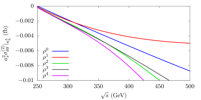
Figure 5: Partonic NNLO $n_{h}^{3}$ cross sections as a function of $\sqrt{s}$; $a_{s}=\alpha_{s}^{(5)}(m_{H})/\pi$.

4 Asymptotic expansion and building blocks

We use this section to describe an important cross check of our calculation, namely the asymptotic expansion performed with exp [7, 8, 9] as compared to the “building-block approach”.

Most of the ingredients needed for the “building-block approach” (introduced in Section 1) can be obtained in a straightforward way. For example, the four-point function involving two gluons and two Higgs bosons can be computed by generating the corresponding four-point amplitude at one and two loops. Since the building block only contains the hard contribution we can Taylor-expand in the three independent external momenta and obtain a power series in $1/m_{t}^{2}$. In the numerator we have all possible scalar products, which can be formed by the external momenta. Note that we have to compute the building blocks for off-shell gluons and Higgs bosons which makes the results quite lengthy. For the $ggHH$ building block the colour factor is given by $\delta^{ab}$ where $a$ and $b$ are the adjoint indices of the gluons. It can be computed separately since colour and Lorentz parts factorize. This statement is true for all building blocks involving up to three gluons but not for the ones involving four gluons.

In the following we consider the class of diagrams which can be described by the four-gluon-two-Higgs building block. There are 3600 such diagrams; a representative five-loop diagram is show in Fig. 6(a). The use of exp for this class of diagrams is straightforward; only one-loop tadpole integrals and a three-loop integral family which corresponds to Fig. 6(b) are needed. The computation of this small set of diagrams is relatively time consuming, requiring a wall-time of 70 hours using TFORM [10] jobs with four cores.

(a)	(b)

Figure 6: (a) Sample Feynman diagram contribution to the NNLO corrections of $gg\to HH$. (b) Feynman diagram which has to be considered in the “building-block-approach”. The pre-expanded 4-gluon-2-Higgs amplitudes have to be inserted at the positions of the blobs.

In the “building-block-approach” approach only one diagram has to be considered which is shown in Fig. 6(b). Since the Lorentz and colour parts do not factorize for the amplitudes involving four (off-shell) gluons we proceed as follows.

First, we compute the one-loop four-gluon-two-Higgs amplitude by simply expanding in the external momenta and arrive at the result

$$B_{4g2H}=\sum_{i}K^{\mu\nu\rho\sigma}_{i}\left(m_{t},\{p_{j}\}\right)C^{abcd}_{i}~{},$$ (5)

where the $K_{i}$ contain all kinematical information and the $C_{i}$ are the colour structures. Note that this quantity has four open Lorentz and four open colour indices. Next, we introduce the symbols $\delta_{i}$ with the properties

$$\delta_{i}\otimes\delta_{j}=\begin{cases}1&i=j\,,\\ 0&i\neq j\,.\end{cases}$$ (6)

This allows us to re-write $B_{4g}$ in the form

$$B_{4g2H}=\left(\sum_{i}K^{\mu\nu\rho\sigma}_{i}\left(m_{t},\{p_{j}\}\right)\delta_{i}\right)\otimes\left(\sum_{j}\delta_{j}C^{abcd}_{j}\right)\,.$$ (7)

In this way we can separate the Lorentz and colour part in the calculation of the diagrams, which involve the building block $B_{4g2H}$ (see, e.g., Fig. 6(b)). Both of them contain the quantities $\delta_{i}$ and Eq. (6) has to be used when Lorentz and colour part are multiplied. Note, that in case we have two building-block insertions with four gluons in one diagram, we introduce two different sets of $\delta_{i}$ which commute with each other.

For the diagram shown in Fig. 6(b), we obtain for the first two expansion terms in $1/m_{t}$

$$\mathrm{D_{\mbox{\tiny Fig.~{}\ref{fig::4g2h}(b)}}}\,\,\sim\,\, \left(\frac{\alpha_{s}}{\pi}\right)^{4}\left(\frac{\mu^{2}}{m_{t}^{2}}\right)^{2\epsilon}\frac{C_{A}^{2}T_{F}^{2}}{N_{A}}\frac{\left(2\epsilon+1\right)\left(2\epsilon-3\right)}{2\left(1-\epsilon\right)^{2}}$$

$$\Bigg{\{}\left[32\left(2\epsilon+1\right)\left(\epsilon-2\right)+\frac{8m_{h}^{2}}{15m_{t}^{2}}\left(\epsilon+1\right)\left(10\epsilon^{2}-31\epsilon-27\right)\right]K_{1}$$

$$+\frac{8m_{h}^{2}}{5m_{t}^{2}}\left(\epsilon+1\right)\left(10\epsilon^{2}-7\epsilon-19\right)K_{2}\Bigg{\}}\,,$$ (8)

where $C_{A}=3$, $T_{F}=1/2$ and $N_{A}=8$ are colour factors and $\mu$ is the renormalization scale. $K_{1}$ and $K_{2}$ are master integrals where $K_{1}$ corresponds to the four-particle phase-space (cf. Fig. 6(b)) and $K_{2}$ has an additional numerator of the form $(m_{h}^{2}-(p_{3}+p_{4})^{2})$, where $p_{3}$ and $p_{4}$ are the momenta of the Higgs bosons.

We use the explicit application of asymptotic expansion to five-loop Feynman diagrams to cross-check the “building-block-approach” at leading order in $1/m_{t}$. For higher order expansion terms it becomes quickly very inefficient which is the reason that we switch to building blocks.

References

- [1] G. Aad et al. [ATLAS Collaboration], Phys. Lett. B 716 (2012) 1 doi:10.1016/j.physletb.2012.08.020 [arXiv:1207.7214 [hep-ex]].
- [2] S. Chatrchyan et al. [CMS Collaboration], Phys. Lett. B 716 (2012) 30 doi:10.1016/j.physletb.2012.08.021 [arXiv:1207.7235 [hep-ex]].
- [3] B. Di Micco et al., arXiv:1910.00012 [hep-ph].
- [4] J. Davies, F. Herren, G. Mishima and M. Steinhauser, JHEP 1905 (2019) 157 [arXiv:1904.11998 [hep-ph]].
- [5] P. Nogueira, J. Comput. Phys. 105 (1993) 279.
- [6] M. Steinhauser, Comput. Phys. Commun. 134 (2001) 335 [arXiv:hep-ph/0009029].
- [7] R. Harlander, T. Seidensticker and M. Steinhauser, Phys. Lett. B 426 (1998) 125 [hep-ph/9712228].
- [8] T. Seidensticker, hep-ph/9905298.
-
[9]
http://sfb-tr9.ttp.kit.edu/software/html/q2eexp.html. - [10] B. Ruijl, T. Ueda and J. Vermaseren, arXiv:1707.06453 [hep-ph].
- [11] T. van Ritbergen, A. N. Schellekens and J. A. M. Vermaseren, Int. J. Mod. Phys. A 14 (1999) 41 [hep-ph/9802376].
- [12] R. N. Lee, arXiv:1212.2685 [hep-ph].
- [13] R. N. Lee, J. Phys. Conf. Ser. 523 (2014) 012059 [arXiv:1310.1145 [hep-ph]].
- [14] J. Grigo, J. Hoff and M. Steinhauser, Nucl. Phys. B 900 (2015) 412 [arXiv:1508.00909 [hep-ph]].
- [15] J. Davies and M. Steinhauser, JHEP 1910 (2019) 166 [arXiv:1909.01361 [hep-ph]].
- [16] A. V. Kotikov, Phys. Lett. B 254 (1991) 158.
- [17] A. V. Kotikov, Phys. Lett. B 259 (1991) 314.
- [18] A. V. Kotikov, Phys. Lett. B 267 (1991) 123 Erratum: [Phys. Lett. B 295 (1992) 409].
- [19] A. B. Goncharov, Math. Res. Lett. 5 (1998) 497 [arXiv:1105.2076 [math.AG]].
- [20] J. M. Henn, Phys. Rev. Lett. 110 (2013) 251601 [arXiv:1304.1806 [hep-th]].
- [21] R. N. Lee, JHEP 1504 (2015) 108 [arXiv:1411.0911 [hep-ph]].
- [22] M. Prausa, Comput. Phys. Commun. 219 (2017) 361 [arXiv:1701.00725 [hep-ph]].
- [23] R. Gröber, A. Maier and T. Rauh, JHEP 1803 (2018) 020 [arXiv:1709.07799 [hep-ph]].