FERMILAB-PUB-21-470-T P3H-21-068 TTP21-034 TU-1133
Real corrections to Higgs boson pair production at NNLO in the large top quark mass limit

Abstract

In this paper we consider the next-to-next-to-leading order total cross section of Higgs boson pair production in the large top quark mass limit and compute four expansion terms in $1/m_{t}^{2}$. Good convergence is observed below the top quark threshold, which makes our results a valuable input for approximation methods which aim for next-to-next-to-leading order corrections over the whole kinematic range. We present details on various steps of our calculation; in particular, we provide results for three- and four-particle phase-space master integrals and describe in detail the evaluation of the collinear counterterms.

1 Introduction

After the discovery of the Higgs boson [1, 2] one of the major tasks of the Large Hadron Collider (LHC) at CERN, and in particular the High-Luminosity LHC, is to investigate the scalar sector of the Standard Model (SM) of particle physics. In principle, within the SM all parameters are known: the scalar potential contains two parameters, the Higgs boson mass ($m_{H}$) and the vacuum expectation value ($v$). Both are available to high precision [3] and their combination determines the triple and quartic Higgs boson couplings via $\lambda=m_{H}^{2}/(2v^{2})\approx 0.13$. However it is important to verify this value of $\lambda$ (and thus the structure of the scalar sector) independently, therefore experimental measurements are crucial.

There are two promising approaches which are sensitive to the value of $\lambda$. Firstly there is double Higgs boson production, where the dominant production process is via gluon fusion. The coupling $\lambda$ already enters at leading order (LO), providing a good sensitivity. On the experimental side, however, a measurement of this cross section with a reasonable precision is very challenging (see, e.g., Refs. [4, 5]). A second process through which information about $\lambda$ can be obtained is single Higgs boson production. The LHC is anticipated to be able to measure this cross section with a precision at the percent level. In the theory predictions, however, $\lambda$ only enters via quantum corrections at next-to-leading order (NLO), reducing the sensitivity to its value in this process.

In this paper we consider double Higgs boson production at next-to-next-to-leading order (NNLO) in the large-$m_{t}$ limit. Special emphasis is put on the real-radiation corrections which to date are only known in the infinite top quark mass limit. We compute finite $1/m_{t}$ corrections up to order $1/m_{t}^{6}$. We describe technical aspects of our calculation in detail, which might be useful for other processes.

Leading order corrections to $gg\to HH$ were first considered more than 30 years ago [6, 7]. At NLO the infinite top quark mass limit is known from [8] and finite $1/m_{t}$ corrections were considered in [9, 10]. At NLO various further approximations have been constructed. Among them is an expansion in the high-energy limit [11, 12], for small transverse momentum of the Higgs bosons [13] and around the top quark threshold [14]. In the latter, the large-$m_{t}$ expansions of the form factors were combined with information from the threshold expansion using conformal mapping and Padé approximation; this produces good approximations of the virtual NLO corrections up to a di-Higgs invariant mass of about $700$ GeV.

Exact NLO corrections for the real-radiation contribution were first obtained in Ref. [15]. The complete exact NLO results are known from Refs. [16, 17, 18], where they are computed using numerical methods. In contrast to the approximations discussed above, which are in general available in analytic from, these numerical computations are quite expensive in terms of CPU time. It is therefore advantageous still to use approximations in the region of the phase space where they are valid. For example in Ref. [19] the exact results from Refs. [16, 17] were combined with the high-energy expansion of Refs. [11, 12]. The CPU-time expensive calculations were only necessary for relatively small values of the Higgs transverse momentum, say below $p_{T}\approx 200$ GeV, and the fast evaluation of the analytic high-energy expansions could be used for the remaining phase space.

The dependence on the renormalization scheme of the top quark mass has been discussed in Ref. [20]. Sizeable uncertainties were observed for large values of the di-Higgs invariant mass. To reduce this uncertainty a NNLO calculation is necessary. A full NNLO calculation is currently out of reach, so it is important to construct approximations valid in different region of the phase space. In the region where the large-$m_{t}$ expansion—the topic of this paper—is valid the scheme uncertainty is small. It is nevertheless useful to have such corrections at hand since they serve as valuable input for approximation methods such as, e.g., the one described in Ref. [14].

At NNLO, only approximations in the large-$m_{t}$ limit are available so far. In the infinite-$m_{t}$ limit the cross section has been computed in Refs. [21, 22, 23] and finite $1/m_{t}$ expansion terms for the virtual corrections are available from [24, 25]. In Ref. [26] a NNLO approximation has been constructed which incorporates, in addition to the exact NLO corrections and the infinite-$m_{t}$ results at NNLO, the exact expression for the double-real radiation contributions at NNLO.

Even N³LO corrections are available for $gg\to HH$, although only in the infinite top quark mass limit. The results presented in Refs. [27, 28] are based on ingredients computed in Refs. [29, 30, 31, 32, 33].

In the present work we consider the $1/m_{t}$ corrections at NNLO. The virtual corrections to the form factors have been computed in [25] including terms to order $1/m_{t}^{8}$. In Section 2.6 we describe our procedure to obtain the corresponding contribution to the cross section to this order. The main purpose of this paper is to complement the virtual corrections by the corresponding real-radiation contributions. We compute all contributions up to order $1/m_{t}^{6}$ and the channels which involve quarks to $1/m_{t}^{8}$.

The real-radiation contribution can be divided into one-loop $2\to 4$ processes and two-loop $2\to 3$ processes; sample Feynman diagrams are shown in Fig. 1. In the following we denote these contributions as “real-real” and “real-virtual”, respectively. We are interested in the total cross section which is conveniently obtained using the optical theorem applied to the forward-scattering amplitude (see Fig. 2). At NNLO this leads to five-loop diagrams. However, in the large-$m_{t}$ limit one observes a factorization into $n$-loop tadpole and $(5-n)$-loop so-called phase-space integrals, where in our case we have $n=2$ or $n=3$. The tadpole integrals are well studied in the literature, however the phase-space integrals are not; we discuss in detail the various integral families, their reduction to master integrals and provide analytic results.

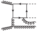
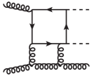
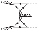
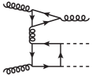
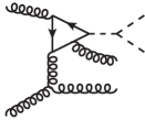
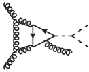
(a)	(b)	(c)	(d)	(e)	(f)

Figure 1: Sample Feynman diagrams contributing to the real radiation. Contributions such as those shown in (c) lead to $n_{h}^{3}$ contributions which have already been computed in Ref. [25]. The $n_{h}^{3}$ contributions of (d) contain a top quark loop without a Higgs coupling and have not been computed in Ref. [25]; they are considered here.

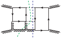
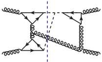
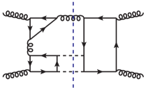
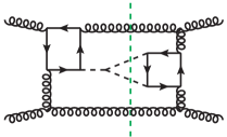
(a)	(b)	(c)	(d)

Figure 2: Sample Feynman diagrams in the forward-scattering kinematics. Three- and four-particle cuts are shown by blue and green dashed lines, respectively. The $n_{h}^{3}$ contributions as shown in (b) have already been considered in [25] but those in (c) have not; they are considered here.

We want to mention that a part of the real-radiation contribution, where the two Higgs bosons couple to different top quark loops (cf. Fig. 1(c)) have been computed in Ref. [25]. In the forward-scattering picture of Fig. 2 such contributions have three closed top quark loops and we denote them the “$n_{h}^{3}$ contribution”. Note that there are further $n_{h}^{3}$ contributions which have a closed loop with only gluon couplings (as shown in Fig. 1(c)). Such terms are not included in Ref. [25], but are computed in this paper.

The remainder of the paper is organized as follows: in the next section we discuss the individual parts of our calculation. This concerns in particular the setup used for the computation of the real-radiation corrections including the asymptotic expansion and the reduction to phase-space master integrals. Furthermore, we discuss the ultraviolet and collinear counterterms to subtract the divergences from initial-state radiation. Section 3 is dedicated to the phase-space master integrals. We provide details on the transformation of the system of differential equations to $\epsilon$ form and on the computation of the boundary conditions in the soft limit. We discuss our analytic and numerical results in Section 4 and summarize our findings in Section 5. In the appendix we provide useful additional material such as explicit formulae used for the computation of the collinear counterterms, the integrands of the phase-space master integrals, NNLO virtual corrections to the channel $q\bar{q}\to HH$ and NNLO virtual corrections involving four closed top quark loops. Furthermore, we describe in detail our approach to obtain the leading $1/m_{t}$ term for double Higgs production from the analytic expressions of the single-Higgs production cross section.

2 Computation

2.1 Partonic channels and generation of amplitudes

We write the perturbative expansion of the partonic cross sections as

$$\sigma_{ij\to HH+X}(s,\rho) = \delta_{ig}\delta_{jg}\sigma_{gg}^{(0)}+\sigma_{ij}^{(1)}+\sigma_{ij}^{(2)}\ldots\,.$$ (1)

where the superscripts (0), (1) and (2) stand for the LO, NLO and NNLO contributions, $s$ is the centre-of-mass energy and $\rho$ is defined in Eq. (4). At NLO and NNLO we further subdivide the cross sections according to the number of closed top quark loops and write

$$\sigma_{ij}^{(1)} = \sigma_{ij}^{(1),n_{h}^{2}}+\delta_{ig}\delta_{jg}\sigma_{gg}^{(1),n_{h}^{3}}\,,$$

$$\sigma_{ij}^{(2)} = \sigma_{ij}^{(2),n_{h}^{2}}+\sigma_{ij}^{(2),n_{h}^{3}}+\delta_{ig}\delta_{jg}\sigma_{gg}^{(2),n_{h}^{4}}\,.$$ (2)

Note that the superscripts $n_{h}^{k}$ counts the number of closed top quark loops which have at least one coupling to a Higgs boson. The contributions $\sigma_{gg}^{(1),n_{h}^{3}}$ and $\sigma_{ij}^{(2),n_{h}^{3}}$ have been computed in Ref. [25]. In this paper we concentrate on $\sigma_{ij}^{(2),n_{h}^{2}}$ which can be decomposed as

$$\sigma_{ij}^{(2),n_{h}^{2}} = \sigma_{ij,\rm virt}^{(2),n_{h}^{2}}+\sigma_{ij,\rm real}^{(2),n_{h}^{2}}+\sigma_{ij,\rm coll}^{(2),n_{h}^{2}}\,,$$ (3)

where the individual contributions are discussed in the remainder of this Section. Most emphasis is put on $\sigma_{ij,\rm real}^{(2),n_{h}^{2}}$ since the complicated calculation for $\sigma_{ij,\rm virt}^{(2),n_{h}^{2}}$ was performed in [25] and for $\sigma_{ij,\rm coll}^{(2),n_{h}^{2}}$ “only” convolutions of lower-order cross sections and splitting functions have to be computed. $\sigma_{gg}^{(2),n_{h}^{4}}$ is discussed in Appendix D.

We compute the cross section in the large-$m_{t}$ limit. It is thus convenient to introduce the variable

$$\rho = \frac{m_{H}^{2}}{m_{t}^{2}}\,,$$ (4)

such that after the expansion in $1/m_{t}$ the coefficients of $\rho^{n}$ depend on $x=m_{H}^{2}/s$. The analytic calculation of the phase-space integrals is performed in an expansion around the production threshold of the two Higgs bosons, for which it is convenient to define

$$\delta = 1-4x\,,$$ (5)

such that the threshold corresponds to $\delta=0$.

To compute $\sigma_{ij,\rm real}^{(2),n_{h}^{2}}$ we first generate the forward-scattering amplitudes for the relevant partonic channels, applying the optical theorem to obtain the real-radiation contributions. These amplitudes involve two external momenta $q_{1}$ and $q_{2}$, with $s=(q_{1}+q_{2})^{2}$. One has to consider the $gg$, $gq$, $q\bar{q}$, $qq$ and $qq^{\prime}$ partonic channels, where $q$ and $q^{\prime}$ denote two different light quark flavours. Note that both quark and anti-quark contributions have to be taken into account, i.e., $gq$ and $qq$ also stand for the $g\bar{q}$ and $\bar{q}\bar{q}$ contributions, respectively. Similarly in $qq^{\prime}$, all quark-quark, quark–anti-quark and anti-quark–anti-quark contributions have to be considered, where in each case the quark flavours are different. For all channels one obtains the same result after replacing a quark by an anti-quark and vice versa. We also compute channels with one or both external gluons replaced with ghosts ($c$) and anti-ghosts ($\bar{c}$), i.e., in addition to the channels listed above we have $gc$, $g\bar{c}$, $cc$, $c\bar{c}$, $\bar{c}\bar{c}$, $cq$ and $\bar{c}q$. This allows us to sum over the gluon polarizations according to

$$\sum_{\lambda}\varepsilon^{(\lambda),*}_{\mu}(q_{1})\varepsilon^{(\lambda)}_{\nu}(q_{2}) = -g_{\mu\nu}\,,$$

where $\lambda$ runs from 0 to 3.

We generate the amplitudes using qgraf [34], however this program does not allow one to filter only diagrams which admit a cut through the required final-state particles (here two Higgs bosons and one or more gluons or light fermion pairs), as depicted in Fig. 2 by the green and blue dashed lines. We thus generate all possible forward-scattering diagrams and post-process them using gen [35] which is able to filter the qgraf output based on our required cuts.

Channel	qgraf diagrams	gen-filtered diagrams	building block diagrams
$gg$	16,631,778	160,154	4,612
$gc$	1,671,006	5,426	336
$c\bar{c}$	406,662	3,879	243
$cc$	(not considered)	(not considered)	8
$gq$	1,671,006	5,426	336
$cq$	(not considered)	(not considered)	8
$q\bar{q}$	406,662	3,879	243
$qq$	(not considered)	(not considered)	8
$qq^{\prime}$	203,331	34	4

Table 1: The number of “full” diagrams generated by qgraf and after filtering with gen, compared to the number of “building block” diagrams, for each channel. For the $cc$, $cq$ and $qq$ channels we have only applied the “building block” approach.

Due to the large qgraf output (for the $gg$ channel, 16.6 million diagrams, 42 GB in total) it proved necessary to separate the diagrams into subsets containing particular numbers of top quark, light quark, cut- and un-cut Higgs lines which could be filtered by gen separately, in parallel. After filtering, the number of diagrams remaining is greatly reduced (for the $gg$ channel, to a total of 160 thousand diagrams, 416 MB in total). In Table 1 we show the numbers of diagrams for all channels which we compute.

2.2 Real radiation: asymptotic expansion and building blocks

After producing the filtered set of Feynman diagrams, we consider the large-$m_{t}$ limit and apply an asymptotic expansion for $m_{t}^{2}\gg s,m_{H}^{2}$. This expresses each diagram as a sum of products of so-called “hard subgraphs” (which have to be expanded in their small quantities: masses and momenta) and “co-subgraphs” which are obtained from the original diagrams by shrinking the subgraph lines to a point. The rules which must be applied to determine all of the relevant subgraphs of a diagram are implemented in the software exp [36, 37], which produces FORM [38] code to perform the expansion.

The subgraphs generated by the asymptotic expansion are, in this case, one- and two-loop one-scale vacuum integrals; this class of integrals is well studied, and it is possible to compute tensor integrals which contract with external momenta or line momenta of the co-subgraph. Such routines are implemented in MATAD [39]. The co-subgraphs of the expansion lead to two- and three-loop forward-scattering integrals (or “phase-space” integrals) which depend on $s$ and $m_{H}^{2}$. The two-loop phase-space integrals involve three-particle cuts whereas the three-loop phase-space integrals involve both three- and four-particle cuts and thus contribute to both the real-virtual and real-real contributions. From the diagrams in Fig. 2 one obtains the diagrams in Fig. 3 where the black circles represent the expanded subgraphs.

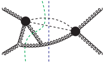
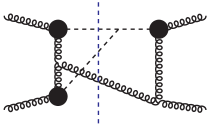
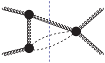
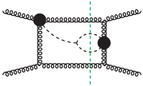
(a)	(b)	(c)	(d)

Figure 3: The forward-scattering diagrams of Fig. 2, with black circles representing the expanded hard subgraphs in the large-$m_{t}$ expansion. Three- and four-particle cuts are shown by blue and green dashed lines, respectively.

In principle, the computation can now be performed using the method and tools described above and in Section 2.1, that is,

1. generate the diagrams with qgraf and filter for valid cuts with gen,

2. use q2e/exp to identify subgraphs and generate FORM code,

3. compute the asymptotic expansion with FORM and MATAD,

yielding expressions in terms of the remaining phase-space integrals which must still be computed. In practice however, this approach is very computationally challenging due to the enormous number of five-loop forward-scattering diagrams generated and the complexity of expanding each of those diagrams due to the large number of propagators present. We use this method to compute in full only the leading contribution to the large-$m_{t}$ expansion (terms of order $1/m_{t}^{0}$) in order to cross-check an alternative approach described below. For the channels $gq$, $q\bar{q}$ and $c\bar{c}$, we additionally perform this cross-check to order $1/m_{t}^{2}$ in the large-$m_{t}$ expansion.

Many of the diagrams have identical subgraphs, which are expanded in the same small parameters. This suggests that it is beneficial to pre-compute the subgraphs, expanding them to the required order only once and storing the results. We can then generate two- and three-loop forward-scattering amplitudes with “effective vertices” in place of the subgraphs, of which there are comparatively very few (for the $gg$ channel we generate 4612 diagrams, compared to the 160 thousand diagrams discussed in Section 2.1. In Table 1 we show the numbers of diagrams for all channels). As an example, in Fig. 4 we show diagrams which involve the 4-gluon–2-Higgs effective vertex; there are 3600 “full” diagrams, one of which is shown in Fig. 4(a), and just one effective-vertex diagram shown in Fig. 4(b). This subset of diagrams has been discussed in Ref. [40]. In the course of the calculation, the effective vertices are replaced with the pre-expanded subgraphs. We call this the “building block approach”.

(a)	(b)

Figure 4: (a) An example “full” Feynman diagram, which contributes to the real-real-virtual corrections of $gg\to HH$. There are 3600 such diagrams. (b) The equivalent “building-block” diagram, of which there is only one.

In practice, we adopt something of a hybrid approach in order to avoid having to deal with two-loop building blocks which are challenging to compute. This means that we implement the following one-loop building blocks: $ggH$, $gggH$, $ggggH$, $ggHH$, $gggHH$, $ggggHH$, shown graphically in Fig. 5. We compute them to order $1/m_{t}^{8}$ with all external momenta off shell, and dependence on the open external Lorentz and colour indices retained. The resulting expressions range between 84 kB for $ggH$ and 164 MB for $ggggHH$. This means that they have to be inserted into the phase-space diagrams carefully, to obtain acceptable performance. Initially the coefficients of each term of the $1/m_{t}^{2}$ expansion are inserted only as placeholder symbols, while the rest of the diagram is computed. Once the expression is written in terms of a linear combination of phase-space integrals, the placeholder symbols are replaced by using Term environments in FORM to sort the coefficients of the phase-space integrals and $1/m_{t}$ expansion coefficients individually, so as not to blow up the intermediate size of the whole expression.

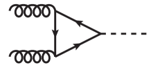
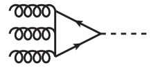
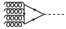
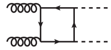
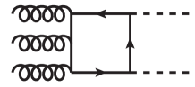
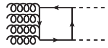
Figure 5: Sample Feynman diagrams contributing to the building blocks.

For the building blocks involving up to three gluons, the Lorentz and colour structures factorise and can thus be inserted separately into the computation of the kinematic and colour parts of the diagrams, as is required by the structure of our setup to compute the diagrams. For the four-gluon building blocks this is no longer the case, so we proceed in the following way. First, we simply compute the expansion of the building blocks to arrive at a result in the form

$$B_{ggggHH}^{\mu\nu\rho\sigma,\,abcd}=\sum_{i}K_{i}^{\mu\nu\rho\sigma}\left(m_{t},\{p_{k}\}\right)\>C_{i}^{abcd}$$ (6)

where the factors $K_{i}$ contain the kinematic dependence. $\{p_{k}\}$ is the set of external momenta of the building block. The colour structures are given by the $C_{i}$ factors. We now define the symbol $\delta_{i}$ such that

$$\delta_{i}\otimes\delta_{j}=\left\{\begin{array}[]{ll}1&i=j\\ 0&i\neq j\\ \end{array}\right.,$$ (7)

which allows us to re-write Eq. (6) as

$$B_{ggggHH}^{\mu\nu\rho\sigma,\,abcd}=\left(\sum_{i}K_{i}^{\mu\nu\rho\sigma}\left(m_{t},\{p_{k}\}\right)\delta_{i}\right)\otimes\left(\sum_{j}\delta_{j}C_{j}^{abcd}\right).$$ (8)

We can thus compute the Lorentz and colour parts of diagrams involving this building block separately, and finally multiply them according to Eq. (7). If a diagram contains two insertions of this building block (such as the diagram shown in Fig. 4) we introduce two independent sets of the $\delta$ symbols.

For diagrams for which the top quark dependence can not be completely constructed from these building blocks (i.e. diagrams which would require two-loop building blocks), we can generate diagrams with at least one (one-loop) building block vertex and treat the remaining top quark propagators explicitly with exp. This means that at most, we have to directly expand the subgraphs of four-loop forward-scattering diagrams. Two examples of such diagrams are shown in Fig. 6. For some diagrams of this type (such as the second example) exp also generates a one-loop subgraph which we discard, since this case is already included in the building block computation.

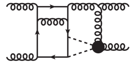
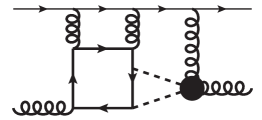
Figure 6: Examples for diagrams for which we perform a direct expansion of the two-loop tadpole subgraph, so as to avoid having to compute two-loop building blocks.

2.3 Real radiation: partial fraction decomposition and IBP reduction

After integrating out the top quark loops we end up with two- and three-loop phase-space integrals. It is useful to distinguish three different sets of integral families according to the number of loops and the cuts through two Higgs bosons and massless particles (see also Fig. 7 below):

• Two-loop families with one or two three-particle cuts. These appear in the real corrections at NLO and real-virtual corrections involving three top quark loops at NNLO.

• Three-loop families with a three-particle cut. These appear in the remaining real-virtual corrections at NNLO.

• Three-loop families with one or two four-particle cuts. These produce the real-real corrections at NNLO.

In total 16 two-loop families, 28 three-loop families with a three-particle cut and 64 four-particle cut families are required to map all diagrams.

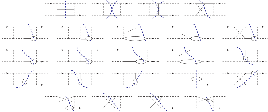
Figure 7: Minimal set of integral families, obtained by LIMIT, for the two-loop (first line), three-loop real-virtual (second line) and three-loop real-real (third to fifth lines) phase-space contributions. The arrow on external lines denotes the momentum $q_{1}$ and the blue dashed lines represent the cuts.

We generate the four-point amplitudes with three independent external momenta, $q_{1}$, $q_{2}$ and $q_{3}$. After using the forward-scattering kinematics, i.e. $q_{3}=-q_{2}$, some of the propagators become linearly dependent; a partial fraction decomposition is needed to obtain proper input for the IBP reduction. For this purpose we have developed the program LIMIT [41] which automates this step of our calculation. This program is based on ideas presented in Ref. [42].

In the following we describe the workflow of LIMIT. First, LIMIT identifies linear relations among the propagators of a given family, derives relations to perform a partial fraction decomposition, and generates FORM routines to apply these relations to the integrals. Each initial, linearly dependent, family may yield multiple linearly independent families.

Next, families with multiple cuts are split into multiple families with one cut each, since each integral with two cuts corresponds to the sum of two integrals with one cut. Splitting the families in this way is necessary because LiteRed [43, 44] can only handle families with a single cut. Now we use LiteRed to identify vanishing sectors of the families and to derive symmetry relations for the non-vanishing sectors. Based on this, LIMIT then generates FORM code to nullify vanishing integrals and apply the symmetry relations, reducing the number of terms present in each amplitude.

Finally, LIMIT identifies equivalent families based on their graph polynomials and groups them into classes. For each class, LiteRed is employed to derive relations for translating integrals of each family to integrals of a single representative family. As not all linearly independent families have the same number of propagators, LIMIT then tries to embed classes of families with fewer lines into classes of families with more lines. The rules for mapping integrals into this minimal number of representative families are translated into FORM code and applied to the amplitudes.

By applying LIMIT to the three sets of integral families mentioned above, we obtain 4, 5 and 14 integral families, respectively. Their graphical representation is shown in Fig. 7. For more details we refer to [41].

Using LiteRed we relate equivalent sectors of families in the three different classes and perform an IBP reduction to master integrals. In total $\mathcal{O}\left(500\,000\right)$ integrals need to be reduced, which takes LiteRed less than two days. The two-loop reduction leads to 16 master integrals with a three-particle cut. They have already been studied in Ref. [25] where the $n_{h}^{3}$ contributions were computed where both Higgs bosons couple to different top-quark loops. We furthermore obtain 17 three-loop three-particle cut and 57 four-particle cut master integrals. They are shown in Fig. 8, as well as Figs. 9 and 10, respectively.

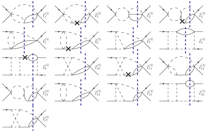
Figure 8: Three-loop three-particle cut master integrals. Solid and dashed lines denote massive and massless lines, respectively. The blue dashed line symbolizes the cut and crosses denote propagators raised to negative power.

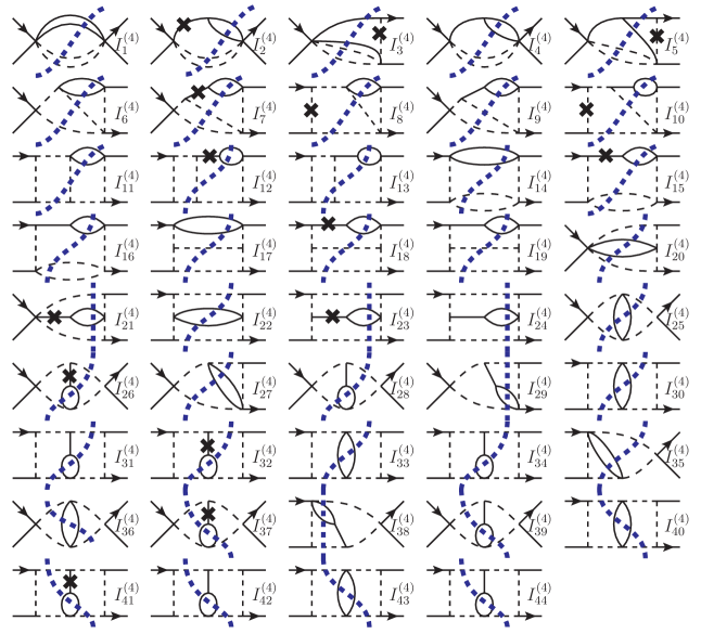
Figure 9: Three-loop four-particle cut master integrals. Solid and dashed lines denote massive and massless lines, respectively. The blue dashed line symbolizes the cut and crosses denote propagators raised to negative power.

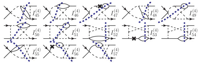
Figure 10: Continuation of Fig. 9.

Details on the computation of the master integrals are provided in Section 3. After inserting the results for the master integrals we obtain an expansion for each Feynman diagram in $1/m_{t}$ and $\epsilon$. For the real-radiation contribution we observe poles of order $1/\epsilon^{4}$.

2.4 Ultraviolet counterterms

The NNLO real-radiation amplitude receives a one-loop counterterm contribution induced by the NLO corrections, which are required to order $\epsilon$. To be more precise, we have to renormalize $\alpha_{s}$, $m_{t}$ and the (external) gluon field. The corresponding renormalization constants are given by

$$Z_{\alpha_{s}} = 1+\frac{\alpha_{s}}{4\pi\epsilon}\left(-\frac{11}{3}C_{A}+\frac{4}{3}n_{f}T_{f}\right),\,$$

$$Z_{m} = 1-\frac{3\alpha_{s}}{4\pi\epsilon}C_{F}\,,\,$$

$$Z_{3}^{\mathrm{OS}} = \frac{1}{\zeta_{3}^{0}}=1-\frac{\alpha_{s}}{3\epsilon\pi}{T_{f}}n_{h}\Bigg{[}1+\epsilon\ln\frac{\mu^{2}}{m_{t}^{2}}+\epsilon^{2}\left(\frac{\zeta_{2}}{2}+\frac{1}{2}\ln^{2}\frac{\mu^{2}}{m_{t}^{2}}\right)$$ (9)

$$\mbox{}+\epsilon^{3}\left(-\frac{\zeta_{3}}{3}+\frac{\zeta_{2}}{2}\ln\frac{\mu^{2}}{m_{t}^{2}}+\frac{1}{6}\ln^{3}\frac{\mu^{2}}{m_{t}^{2}}\right)+\mathcal{O}(\epsilon^{4})\Bigg{]},$$

where $\mu$ is the renormalization scale and $\alpha_{s}=\alpha_{s}(\mu)$. We first perform the renormalization in the full theory (i.e., we have $n_{f}=6=n_{l}+n_{h}=5+1$). Afterwards, we perform a decoupling from $\alpha_{s}^{(6)}$ to $\alpha_{s}^{(5)}$. Note that we renormalize the top quark mass first in the $\overline{\mathrm{MS}}$ scheme; the transition to the on-shell scheme in the final result is straightforward.

2.5 Collinear counterterms

The NNLO collinear counterterms are obtained from the convolution of the LO and NLO cross sections $\sigma_{gg}^{(0)}$ and $\sigma_{ij}^{(1)}$ and the gluon or quark splitting functions. In general such a convolution has the form

$$\frac{\sigma_{ij}^{\rm bare}(x)}{x} = \sum_{k,l}\frac{\sigma_{{kl}}(z)}{z}\otimes\Gamma_{ki}\otimes\Gamma_{lj}\,,$$ (10)

with

$$(f\otimes g)(z) = \int_{0}^{1}{\rm d}x\,{\rm d}y\,f(x)g(y)\delta(z-xy)\,.$$ (11)

In Eq. (10) the superscript “bare” refers to the renormalization of the parton distribution functions, i.e. the subtraction of the $1/\epsilon$ poles in connection to radiation from incoming partons. It does not refer to the renormalization of the ultraviolet divergences; here we assume that all ultraviolet counterterms are already taken into account. The kernels $\Gamma_{ij}$ in Eq. (10) are obtained from the splitting functions as follows

$$\Gamma_{ij}(x) = \delta_{ij}\delta(1-x)-\frac{\alpha_{s}^{(5)}(\mu)}{\pi}\frac{P_{ij}^{(0)}}{\epsilon}$$ (12)

$$+\left(\frac{\alpha_{s}^{(5)}(\mu)}{\pi}\right)^{\!2}\!\!\left\{\frac{1}{2\epsilon^{2}}\left[\left(P_{ik}^{(0)}\otimes P_{kj}^{(0)}\right)(x)+\beta_{0}P_{ij}^{(0)}\right]-\frac{1}{2\epsilon}P_{ij}^{(1)}\right\}+\mathcal{O}\left(\alpha_{s}^{3}\right),$$

where $P_{ij}^{(0)}$ and $P_{ij}^{(1)}$ are one- and two-loop splitting functions which can be found in Refs. [45, 46, 47, 48]. For further details we refer to Refs. [49, 50] where the computation of the collinear counterterms is discussed for NNLO and N³LO single Higgs boson production. The combinatorics for single and double Higgs production is identical and thus the formalism outlined in detail in [49] can be applied in the context of this calculation. Additionally, this reference contains explicit formulae which solve Eq. (10) for the renormalized cross section $\sigma_{ij}$ within perturbation theory. The resulting collinear counterterms are computed from convolution integrals of the following form,

$$\sigma_{gg,\rm coll}^{(2)} = -\frac{1}{\epsilon}\left(\frac{\mu^{2}}{\mu_{f}^{2}}\right)^{\epsilon}\int_{1-\delta}^{1}\mathrm{d}z\,P^{(0)}_{gg}(z)\sigma_{gg}^{(1)}(x/z)+\ldots\,,$$ (13)

where the ellipses represent further contributions to the collinear NNLO counterterm $\sigma_{gg,\rm coll}^{(2)}$. Note that in Eq. (13) we distinguish the renormalization scale $\mu$ from the factorization scale $\mu_{f}$. We compute the collinear counterterms in the $n_{l}$ flavour theory, i.e., in Eq. (12) the one-loop coefficient of the QCD beta function is given by

$$\beta_{0} = \frac{11}{12}C_{A}-\frac{1}{3}T_{f}{n_{l}}\,,$$ (14)

where $n_{l}$ is the number of massless quarks. We compute all contributions in terms of SU$(N_{c})$ colour factors $C_{A}=N_{c}$ and $C_{F}=(N_{c}^{2}-1)/(2N_{c})$ and the trace normalization $T_{f}=1/2$.

Inspection of Eq. (12) shows that at NNLO the collinear counterterm starts at $\mathcal{O}(1/\epsilon^{2})$ whereas the real and virtual corrections contain poles up to $\mathcal{O}(1/\epsilon^{4})$. In Appendix A we provide useful formulae for the analytic computation of the convolution integrals, such as the one shown in Eq. (13). These are obtained by expanding in $\delta$; we have computed all contributions up to order $\rho^{3}$ and $\delta^{30}$.

2.6 Virtual corrections

(a) LO	(b) NLO, $n_{h}^{2}$	(c) NLO, $n_{h}^{3}$	(d) NNLO, $n_{h}^{2}$
(e) NNLO, $n_{h}^{2}$	(f) NNLO, $n_{h}^{3}$	(g) NNLO, $n_{h}^{3}$	(h) NNLO, $n_{h}^{4}$

Figure 11: Sample forward-scattering Feynman diagrams for the virtual corrections at LO, NLO and NNLO.

Virtual corrections only exist for the $gg$ and $q\bar{q}$ channels. In the latter case they contribute for the first time at NNLO and are suppressed by $1/m_{t}^{2}$ at the level of the amplitude (and so by $1/m_{t}^{4}$ at the level of the cross section). We discuss them in Appendix C. In this section we concentrate on the channel $gg\to HH$. Sample Feynman diagrams for the forward-scattering kinematics are shown in Fig. 11. At NNLO we distinguish contributions which have two, three and four closed top quark loops and we denote the corresponding contributions by $n_{h}^{2}$, $n_{h}^{3}$ and $n_{h}^{4}$ respectively. Note that all $n_{h}^{3}$ virtual corrections are already contained in Ref. [25], even those with a top quark loop which has no coupling to the Higgs bosons (such as the diagram in Fig. 11(g)). The $n_{h}^{2}$ terms develop poles up to $1/\epsilon^{4}$ which cancel against those of the real-radiation corrections. The $n_{h}^{4}$ contribution appears only in the virtual corrections and is therefore finite. The corresponding analytic results are presented in Appendix D.

For the virtual corrections we do not use the optical theorem but compute the contribution to the cross section from the form factors obtained in Ref. [51] in an expansion up to order $1/m_{t}^{8}$. The triangle form factors are even available up to order $1/m_{t}^{14}$.

The starting point is the amplitude for the process $gg\to HH$ which has two independent tensor structures. Expressed in terms of the “box” and “triangle” form factors it is given by

$$\delta^{ab}{\cal M} = \delta^{ab}\>\varepsilon_{1,\mu}\varepsilon_{2,\nu}\>\frac{G_{F}}{\sqrt{2}}\frac{\alpha_{s}(\mu)}{2\pi}T_{f}n_{h}\,s\,\left[\left(\frac{3m_{H}^{2}}{s-m_{H}^{2}}F_{\rm tri}+F_{\rm box1}\right)A_{1}^{\mu\nu}+F_{\rm box2}A_{2}^{\mu\nu}\right],$$ (15)

where $G_{F}$ is the Fermi constant, $a$ and $b$ are adjoint colour indices and the two Lorentz structures are given by

$$A_{1}^{\mu\nu} = g^{\mu\nu}-{\frac{1}{q_{12}}q_{1}^{\nu}q_{2}^{\mu}}\,,$$

$$A_{2}^{\mu\nu} = g^{\mu\nu}+\frac{1}{p_{T}^{2}q_{12}}\left(q_{33}q_{1}^{\nu}q_{2}^{\mu}-2q_{23}q_{1}^{\nu}q_{3}^{\mu}-2q_{13}q_{3}^{\nu}q_{2}^{\mu}+2q_{12}q_{3}^{\mu}q_{3}^{\nu}\right)\,,$$ (16)

with

$$q_{ij} = q_{i}\cdot q_{j}\,,\qquad p_{T}^{\>2}\>\>\>=\>\>\>\frac{2q_{13}q_{23}}{q_{12}}-q_{33}\,.$$ (17)

Analytic results for the form factors $F_{\rm tri}$, $F_{\rm box1}$, $F_{\rm box2}$ are available in the ancillary files of Ref. [51].

The differential cross section is constructed in terms of the amplitude of Eq. (15) according to

$$\frac{{\rm d}\sigma}{{\rm d}{y}} = \frac{N_{A}}{2\cdot N_{A}^{2}\cdot(2-2\epsilon)^{2}}{\frac{1}{2s}}f^{\rm 2PS}(\epsilon)\left|{\cal M}^{\star}{\cal M}\right|$$ (18)

where the factors $1/2$, $1/N_{A}^{2}=1/8^{2}$ and $1/(2-2\epsilon)^{2}$ are due to the identical particles in the final state, and the gluon colour and spin averages, respectively. The factor $f^{\rm 2PS}$ comes from the $d$-dimensional two-particle phase space and is given by

$$f^{\rm 2PS}(\epsilon) = \left(\frac{e^{\gamma_{E}}}{4\pi}\right)^{\epsilon}\left(\frac{\mu^{2}}{s}\right)^{\epsilon}\frac{2^{2\epsilon-3}\>\>\pi^{\epsilon-1}\>\>\delta^{1/2-\epsilon}}{\Gamma(1-\epsilon)}\left(y(1-y)\right)^{-\epsilon}.$$ (19)

We perform the integration to obtain the cross section after expanding in $\delta$. If we were to integrate over $t$, the integration boundaries would be $\delta$ dependent. We therefore make the following change of variables:

$$t \to -\frac{s}{4}\left(1+\delta-4y\sqrt{\delta}+2\sqrt{\delta}\right)\,.$$ (20)

In terms of the new integration variable $y$ the integration boundaries become $[0,1]$ and the $\delta$ dependence is isolated to the integrand. This allows us to expand in $\delta$ at the level of the integrand, and thus integrate each term of the expansion individually. In the supplementary material to this paper we provide the results in such a way that the (divergent) virtual corrections can be extracted.

We perform the construction described above for the ultraviolet renormalized form factors as published in Ref. [51]. The renormalization of the gluon wave function, top quark mass and strong coupling in the LO expression induces $1/\epsilon$ poles at NLO and $1/\epsilon^{2}$ poles at NNLO. The insertion of the one-loop counterterms in the virtual NLO expression (which has an $\epsilon$ expansion starting at $1/\epsilon^{2}$) induces $1/\epsilon^{3}$ poles at NNLO.

3 Phase-space master integrals

3.1 Transformation to $\epsilon$ form

In this section, we discuss the computation of the 17 three-loop three-particle cut master integrals depicted in Fig. 8, as well as the 57 three-loop four-particle cut master integrals depicted in Figs. 9 and 10. We follow the method of differential equations [52, 53] and use LiteRed to take the derivative of each master integral w.r.t. $x$ and reduce the resulting integrals back to master integrals. Thus, we obtain two systems of differential equations: one for the three-particle cut integrals and one for the four-particle cut integrals. These systems have the form

$$\partial_{x}\vec{L}=M\!\left(x,\epsilon\right)\,\vec{L}~{}.$$ (21)

$\vec{L}$ is the vector of master integrals, and the matrix $M$ is block-triangular with entries rational in both $x$ and $\epsilon$. In the following we take two approaches to solve Eq. (21): in Section 3.2 we seek a canonical basis of master integrals [54] and in Section 3.3 we compute them in terms of an asymptotic series in $\delta$.

3.2 Finding a canonical basis

A canonical basis $\vec{C}$ is a particularly useful basis of integrals in which the differential equations take the form

$$\partial_{x}\vec{C}=\epsilon\sum_{i}\frac{{\hat{M}_{i}}}{x-x_{i}}\vec{C}~{},$$ (22)

where the $x_{i}$ are constants and the matrices $\hat{M}_{i}$ do not depend on $\epsilon$ or $x$. A system of the form of Eq. (22) can be integrated order-by-order in $\epsilon$ in terms of Goncharov Polylogarithms (GPLs) [55] over the letters $x_{i}$.

To find a rational transformation from $\vec{L}$ to $\vec{C}$ we use the program Libra [56] and adapt Lee’s algorithm [57] to the problem at hand. As the matrix $M(x,\epsilon)$ contains rational functions with numerator and denominator degrees as high as $20$ in our case, a direct application of Lee’s algorithm would lead to unmanageable intermediate expression swell. We thus deviate from the standard algorithm by first bringing all diagonal blocks to Fuchsian form (that is, they have only simple poles in $x$), followed by bringing the off-diagonal blocks to Fuchsian form. We then normalize the eigenvalues of all residues to be proportional to $\epsilon$ or take the form $a\epsilon\pm 1/2$, where $a$ is an integer.

Consequently, we arrive at an intermediate basis $\vec{I}$, related to $\vec{L}$ by a rational transformation, in which the differential equations are in Fuchsian form and do not contain spurious poles:

$$\partial_{x}\vec{I}=\sum_{i}\frac{\tilde{M}_{i}(\epsilon)}{x-x_{i}}\vec{I}~{}.$$ (23)

For the three-particle cut master integrals the poles $x_{i}$ are given by $0$, $1/4$ and $1$, corresponding to the kinematic limits $s\rightarrow\infty$, $s\rightarrow 4m_{H}^{2}$ and $s\rightarrow m_{H}^{2}$, respectively. In the case of the four-particle cut master integrals there are also poles at $-1/4$ and $-1$, corresponding to the kinematic limits $s\rightarrow-4m_{H}^{2}$ and $s\rightarrow-m_{H}^{2}$ respectively.

Rational transformations render the eigenvalues of all poles proportional to $\epsilon$, apart from $\pm 1/4$. Therefore to find a canonical basis, we need to rationalize the square roots $\sqrt{1-4x}$ and $\sqrt{1+4x}$. For the three-particle cut master integrals only the first square root plays a role. For this system, we perform the variable change

$$x=\frac{z}{(z+1)^{2}}$$ (24)

mapping the physical interval $x\in[1/4,0)$ to $z\in[1,0)$. In the case of the four-particle cut master integrals we need to rationalize both square roots simultaneously, requiring the more complicated variable change

$$x =\frac{k^{4}-6k^{2}+1}{4(1+k^{2})^{2}}~{}.$$ (25)

This change maps $x\in[1/4,0)$ to $k\in[0,\sqrt{2}-1)$.

With all roots rationalized, we now proceed by normalizing the corresponding eigenvalues to be proportional to integers, bringing the off-diagonal blocks into Fuchsian form once more and factoring out $\epsilon$ to arrive at a canonical basis in $z$ and $k$ for the three- and four-particle cut systems, respectively. These resulting system can be integrated in terms of GPLs and their boundary conditions can be fixed in the limit $x\rightarrow 1/4$.

Once we have the leading-order term in the $\delta$ expansion for the master integrals (see Section 3.3), the exact expressions for the master integrals can be computed in two ways. The first is to transform the leading-$\delta$ terms of all master integrals into the canonical basis. The differential system can then be integrated order-by-order in $\epsilon$ and the integration constants are fixed by comparing the resulting expressions to the boundary conditions in the limit $\delta\rightarrow 0$.

The second option is to first compute the path-ordered exponential $U$ of the canonical differential equation matrix $M$

$$U=\mathcal{P}\exp\left[\epsilon\int\mathrm{d}x\>{\sum_{i}\frac{\hat{M}_{i}}{(x-x_{i})}}\right]~{},$$ (26)

in terms of which we can write the master integrals of the canonical basis as

$$\vec{I}(x)=U\vec{I}_{0}~{},$$ (27)

where $\vec{I}_{0}$ does not depend on $x$. Libra can decompose $\vec{I}_{0}$ as

$$\vec{I}_{0}={K(\epsilon)}\>\vec{c}~{},$$ (28)

where $K$ depends only on $\epsilon$ and $\vec{c}$ is the minimal number of necessary boundary conditions. The entries of $\vec{c}$ are given by the leading-order terms in the $\delta$ expansion of a certain subset of original master integrals, determined by Libra to be sufficient to fix all boundary conditions.

The main difference between these two approaches is the apparent number of necessary boundary conditions. For example using the first approach, we need the integrals $I_{1}^{(4)}$, $I_{2}^{(4)}$ and $I_{3}^{(4)}$ to determine $I_{1}^{(4)},\ldots,I_{10}^{(4)}$, whereas Libra finds that $I_{1}^{(4)}$ is sufficient. Thus, it makes use of relations among the leading-$\delta$ terms of different integrals.

In our calculation we have used both methods for the three-loop three-particle cut master integrals. For the three-loop four-particle cut master integrals we have only used the first method since our non-trivial letters make the construction of the matrix $U$ difficult.

In the following section we describe how we compute the boundary conditions. We will compute the leading-order term in the $\delta$ expansion for all master integrals; the integrals which are not necessary to integrate the differential system serve as a cross check.

3.3 Computation of the boundary conditions

In the previous subsection we have presented the construction of the exact results for the phase-space master integrals. The purpose of this subsection is to provide boundary conditions needed to compute the exact expressions. In the next subsection we briefly describe a formalism which allows us to compute the $\delta$ expansion of all master integrals to a high enough order in $\delta$ to be sufficient for practical applications. In fact, in the combination of the real-radiation contribution with the virtual corrections and the collinear counterterm it is necessary to use the $\delta$-expanded results in order check the cancellation of the $\epsilon$ poles analytically.

We start with some definitions which are common to the three- and four-particle phase-space integrals. For the phase-space measures of the Higgs bosons we write

$$\mathcal{D}p_{j}\equiv\frac{\mathrm{d}^{d-1}p_{j}}{(2\pi)^{d-1}}\frac{1}{2E_{j}}=\frac{p_{j}^{d-2}\mathrm{d}p_{j}}{(2\pi)^{d-1}}\frac{1}{2E_{j}}\mathrm{d}\Omega_{d-1}^{(j)}\qquad\mathrm{with}\quad j=3,4\,,$$ (29)

and the phase-space measures of massless particles are given by

$$\mathcal{D}p_{j}\equiv\frac{1}{2}\frac{p_{j}^{d-3}\mathrm{d}p_{j}}{(2\pi)^{d-1}}\mathrm{d}\Omega_{d-1}^{(j)}\qquad\mathrm{with}\quad j=5,6\,.$$ (30)

When necessary, we use a parametrization for the momenta such that the scalar products take the form

$$q_{1}\cdot p_{5}=\frac{s}{4}\kappa_{5}(1-\cos\theta_{5}), \quad q_{2}\cdot p_{5}=\frac{s}{4}\kappa_{5}(1+\cos\theta_{5}),$$

$$q_{1}\cdot p_{6}=\frac{s}{4}\kappa_{6}(1-\cos\theta_{6}), \quad q_{2}\cdot p_{6}=\frac{s}{4}\kappa_{6}(1+\cos\theta_{6})\,,$$

$$q_{1}\cdot(p_{5}+p_{6})=\frac{s}{4}\kappa_{56}(1-\cos\theta_{56}), \quad q_{2}\cdot(p_{5}+p_{6})=\frac{s}{4}\kappa_{56}(1+\cos\theta_{56})\,,$$ (31)

where $q_{i}$ and $p_{j}$ are momenta of the initial and final state, respectively.

In the following, we use the symbol “$\approx$” to denote that the leading-order term in $\delta$ expansion agrees on the the left- and right-hand sides of the equation, but that the sub-leading terms may differ.

For the $(d-1)$-dimensional angular integration, we use the following property:

$$\int\mathrm{d}\Omega_{d-1}^{(j)} =\frac{2\pi^{\frac{d-3}{2}}}{\Gamma\left(\frac{d-3}{2}\right)}\int_{-1}^{1}\left(1-\cos^{2}\theta_{j}\right)^{\frac{d-4}{2}}\mathrm{~{}d}\cos\theta_{j}\int_{-1}^{1}\left(1-\cos^{2}\phi_{j}\right)^{\frac{d-5}{2}}\mathrm{~{}d}\cos\phi_{j}=\frac{2\pi^{\frac{d-1}{2}}}{\Gamma\left(\frac{d-1}{2}\right)}\,.$$ (32)

3.3.1 Three-particle phase space

All 17 three-particle cut master integrals can be written as

$$I_{i}^{(3)}=\left(\frac{e^{\gamma_{E}}\mu^{2}}{4\pi}\right)^{3\epsilon}\int\mathcal{D}p_{3}\mathcal{D}p_{4}\mathcal{D}p_{5}\>(2\pi)^{d}\>\delta^{(d)}\!\left(q_{1}+q_{2}-p_{3}-p_{4}-p_{5}\right)\mathcal{Q}_{i}^{(3)}\,,$$ (33)

where $\mathcal{Q}_{i}^{(3)}$ are one-loop integrals, which can easily be read off from Fig. 8. For convenience we provide explicit expressions in Appendix E. Note that the $\mathcal{Q}^{(3)}_{i}$ do not depend on $p_{3}$ and $p_{4}$, since the external momenta of the loop diagrams are $q_{1},q_{2},p_{5}$ and the combination $p_{3}+p_{4}$. The latter can be eliminated by using momentum conservation. By performing the integration over $p_{4}$ and taking the leading order in $\delta$, we obtain

$$I_{i}^{(3)}\approx\left(\frac{e^{\gamma_{E}}\mu^{2}}{4\pi}\right)^{3\epsilon}\int\mathcal{D}p_{3}\mathcal{D}p_{5}\frac{4\pi}{s}\>\delta\!\left(\delta-\frac{\vec{p}_{3}^{\,\,2}}{m_{H}^{2}}-\kappa_{5}\right)\mathcal{Q}_{i}^{(3)}$$ (34)

which indicates

$$|\vec{p}_{3}|\leq m_{H}\sqrt{\delta},\quad\kappa_{5}\leq\delta\,.$$ (35)

There are six one-loop integrals appearing in the 17 master integrals. Three of them ($L_{1},L_{2},L_{3}$) are massless one-loop two-point functions and are known for a general dimension $d$:

$$L_{1} =\int\frac{\mathrm{d}^{d}\ell}{i(2\pi)^{d}}\>\frac{1}{-(\ell+p_{5})^{2}}\>\frac{1}{-(\ell+q_{1}+q_{2})^{2}}\approx\frac{1}{(4\pi)^{2-\epsilon}}\frac{\Gamma(1-\epsilon)^{2}\Gamma(\epsilon)}{\Gamma(2-2\epsilon)}s^{-\epsilon}e^{i\epsilon\pi}\,,$$

$$L_{2} =\int\frac{\mathrm{d}^{d}\ell}{i(2\pi)^{d}}\>\frac{1}{-\ell^{2}}\>\frac{1}{-(\ell+q_{1}+q_{2})^{2}}=\frac{1}{(4\pi)^{2-\epsilon}}\frac{\Gamma(1-\epsilon)^{2}\Gamma(\epsilon)}{\Gamma(2-2\epsilon)}s^{-\epsilon}e^{i\epsilon\pi}\approx L_{1}\,,$$

$$L_{3} =\int\frac{\mathrm{d}^{d}\ell}{i(2\pi)^{d}}\>\frac{1}{-(\ell+p_{5})^{2}}\>\frac{1}{-(\ell+q_{1})^{2}}\approx\frac{1}{(4\pi)^{2-\epsilon}}\frac{\Gamma(1-\epsilon)^{2}\Gamma(\epsilon)}{\Gamma(2-2\epsilon)}\frac{2^{\epsilon}}{(s(1-\cos\theta_{5})\kappa_{5})^{\epsilon}}\,.$$ (36)

Note that in the soft limit there are only five independent one-loop integrals since $L_{2}\approx L_{1}$. The remaining three integrals ($L_{4},L_{5},L_{6}$) are either triangle or box diagrams, and their soft limit can be computed using expansion by regions [58, 59, 60]. In particular, we use the implementation in the Mathematica package asy2.m [60]. Applying this method is straightforward but the details of the computation are rather technical; we do not discuss them here but simply refer to Ref. [60]. Rather, in this paper, we discuss an alternative way to obtain the same results by making use of the Mellin-Barnes representation, which serves as a cross-check of the calculation based on expansion by regions. In the following, it is assumed that the integration contours of the Mellin-Barnes integrals are chosen properly, (see, e.g., Ref. [61]) and we abbreviate the product of $\Gamma$-functions as

$$\Gamma\left[x_{1},\ldots,x_{n}\right]\equiv\prod_{i=1}^{n}\Gamma\left(x_{i}\right)\,.$$ (37)

We begin by expressing the integrals in the Mellin-Barnes representation:

$$L_{4} =\int\frac{\mathrm{d}^{d}\ell}{i(2\pi)^{d}}\>\frac{1}{-(\ell+p_{5})^{2}}\>\frac{1}{-(\ell+q_{1})^{2}}\>\frac{1}{-(\ell+q_{1}+q_{2})^{2}}$$ (38)

$$=\frac{-e^{i\pi\epsilon}}{(4\pi)^{2-\epsilon}}\int\mathrm{d}z_{1}\mathrm{d}z_{2}\frac{\kappa_{5}^{z_{1}}e^{i\pi z_{1}}\Gamma[-z_{2},z_{2}+1,-\epsilon,z_{2}-z_{1},z_{1}+\epsilon+1,-z_{2}-\epsilon]}{2^{z_{2}}s^{\epsilon+1}(1-\cos\theta_{5})^{-z_{2}}\Gamma(1-2\epsilon)}\,,$$

$$L_{5} =\int\frac{\mathrm{d}^{d}\ell}{i(2\pi)^{d}}\>\frac{1}{-\ell^{2}}\>\frac{1}{-(\ell+p_{5})^{2}}\>\frac{1}{-(\ell+q_{2})^{2}}\>\frac{1}{-(\ell+q_{1}+q_{2})^{2}}$$

$$=\frac{e^{i\pi\epsilon}}{(4\pi)^{2-\epsilon}}\int\mathrm{d}z_{1}\mathrm{d}z_{2}\frac{\kappa_{5}^{z_{1}}e^{i\pi z_{1}}\Gamma[z_{1}+1,-z_{2},z_{2}+1,-\epsilon,z_{2}-z_{1},z_{1}+\epsilon+2,-z_{2}-\epsilon-1]}{2^{z_{2}+1}s^{\epsilon+2}(1+\cos\theta_{5})^{-z_{2}}\Gamma[z_{1}+2,-2\epsilon]}\,,$$

$$L_{6} =\int\frac{\mathrm{d}^{d}\ell}{i(2\pi)^{d}}\>\frac{1}{-\ell^{2}}\>\frac{1}{-(\ell+q_{1})^{2}}\>\frac{1}{-(\ell-p_{5}+q_{1})^{2}}\>\frac{1}{-(\ell-p_{5}+q_{1}+q_{2})^{2}}$$

$$=\frac{e^{i\pi\epsilon}}{(4\pi)^{2-\epsilon}}\int\mathrm{d}z_{1}\mathrm{d}z_{2}\frac{\kappa_{5}^{z_{1}}e^{i\pi z_{1}}\Gamma[-z_{2},-\epsilon,-\epsilon,z_{2}-z_{1},z_{1}+\epsilon+2,-z_{2}-\epsilon-1]}{2^{z_{1}+1}s^{\epsilon+2}(1+\cos\theta_{5})^{-z_{2}}(1-\cos\theta_{5})^{-z_{1}+z_{2}}\Gamma[-2\epsilon,-z_{2}-\epsilon]}$$

$$\qquad\times\frac{\Gamma(z_{2}-z_{1}-\epsilon-1)}{\Gamma(-z_{1}+z_{2}-\epsilon)}\,.$$

Note that the Mellin-Barnes representation of a given Feynman integral is not unique; here we show the representations used in our calculation. We choose them in such a way that the exponent of $\kappa_{5}$ is $z_{1}$. From Eq. (35), we see that the leading-order term in $\delta$ is obtained from the leading-order term in $\kappa_{5}$. We solve $z_{1}$ integrals above by closing the integration contour in the right half plane and taking the residues of the poles of $\Gamma$-functions. For example, in $L_{5}$ only the poles of $\Gamma(z_{2}-z_{1})$ contribute and their locations are $z_{1}=z_{2}-n$ where $n=0,1,2,...$. Thus the leading order in $\kappa_{5}$ corresponds to $z_{1}=z_{2}$ pole. Keeping this in mind, we first solve the $z_{2}$ integral also by closing the integration contour in its right half plane. This time, the poles from $\Gamma(-z_{2})$ and $\Gamma(-z_{2}-\epsilon-1)$ contribute. Among these, the pole at $z_{2}=-\epsilon-1$ gives the smallest value of $z_{2}$, so we consider the residue at this pole. The resulting expression is now a one-dimensional integral over $z_{1}$, and its leading-order term in $\kappa_{5}$ is obtained by taking the residue at $z_{1}(=z_{2})=-\epsilon-1$. In this way, we extract the leading-order term of $L_{5}$ in $\kappa_{5}$. The calculation of $L_{4}$ and $L_{6}$ proceeds in a similar way. For $L_{4}$, the two poles at $z_{2}=0$ and $z_{2}=-\epsilon$ contribute to the leading order and we have to take both of them into account. For $L_{6}$, the leading-order term is obtained from the pole at $z_{1}=z_{2}-\epsilon-1$ instead of $z_{1}=z_{2}$. The results are given by

$$L_{4} \approx\frac{1}{(4\pi)^{2-\epsilon}}\frac{\Gamma(1+\epsilon)\Gamma(-\epsilon)^{2}\left(2^{\epsilon}(1-\cos\theta_{5})^{-\epsilon}\kappa_{5}^{-\epsilon}-e^{i\pi\epsilon}\right)}{s^{\epsilon+1}\Gamma(1-2\epsilon)\Gamma(\epsilon+1)}\,,$$

$$L_{5} \approx\frac{-1}{(4\pi)^{2-\epsilon}}\frac{2^{\epsilon}(\cos\theta_{5}+1)^{-\epsilon-1}\kappa_{5}^{-\epsilon-1}\Gamma(-\epsilon)^{2}\Gamma(\epsilon)}{s^{\epsilon+2}\Gamma(-2\epsilon)}\,,$$

$$L_{6} \approx\frac{1}{(4\pi)^{2-\epsilon}}\frac{2^{2\epsilon+1}e^{-i\pi\epsilon}\left(1-\cos\theta_{5}^{2}\right)^{-\epsilon-1}\kappa_{5}^{-2(\epsilon+1)}\Gamma(-\epsilon)^{3}\Gamma(\epsilon+1)^{2}}{s^{\epsilon+2}\Gamma(-2\epsilon)}\,.$$ (39)

We follow Ref. [25] to perform the three-particle phase-space integration and obtain the following results for the leading-$\delta$ contribution of the master integrals:

$$I^{(3)}_{1} \approx\delta^{5/2}\left[\frac{s}{7680\pi^{5}\epsilon}-\frac{s(15\log\delta-56+20\log 2)}{38400\pi^{5}}+\mathcal{O}(\epsilon^{1})\right]\,,$$

$$I^{(3)}_{2} \approx\delta^{5/2}\left[-\frac{s^{2}}{10240\pi^{5}\epsilon}+\frac{s^{2}(15\log\delta-56+20\log 2)}{51200\pi^{5}}+\mathcal{O}(\epsilon^{1})\right]\,,$$

$$I^{(3)}_{3} \approx\delta^{5/2}\left[\frac{s}{7680\pi^{5}\epsilon}-\frac{s(15\log\delta-56+20\log 2)}{38400\pi^{5}}+\mathcal{O}(\epsilon^{1})\right]\,,$$

$$I^{(3)}_{4} \approx\delta^{5/2}\left[-\frac{s^{2}}{10240\pi^{5}\epsilon}+\frac{s^{2}(15\log\delta-56+20\log 2)}{51200\pi^{5}}+\mathcal{O}(\epsilon^{1})\right]\,,$$

$$I^{(3)}_{5} \approx\delta^{5/2}\left[\frac{s}{7680\pi^{5}\epsilon}-\frac{s(30\log\delta-107+45\log 2)}{57600\pi^{5}}+\mathcal{O}(\epsilon^{1})\right]\,,$$

$$I^{(3)}_{6} \approx\delta^{5/2}\left[-\frac{s^{2}}{10240\pi^{5}\epsilon}+\frac{s^{2}(30\log\delta-107+45\log 2)}{76800\pi^{5}}+\mathcal{O}(\epsilon^{1})\right]\,,$$

$$I^{(3)}_{7} \approx\delta^{5/2}\left[\frac{-15\log\delta+46-30\log 2}{115200\pi^{5}\epsilon}+\mathcal{O}(\epsilon^{0})\right]\,,$$

$$I^{(3)}_{8} \approx\sqrt{\delta}\left[-\frac{1}{2048\pi^{5}s^{2}\epsilon^{4}}+\frac{2\log\delta-4+3\log 2}{1024\pi^{5}s^{2}\epsilon^{3}}+\mathcal{O}(\epsilon^{-2})\right]\,,$$

$$I^{(3)}_{9} \approx\sqrt{\delta}\left[\frac{3}{8192\pi^{5}s\epsilon^{4}}-\frac{3(2\log\delta-4+3\log 2)}{4096\pi^{5}s\epsilon^{3}}+\mathcal{O}(\epsilon^{-2})\right]\,,$$

$$I^{(3)}_{10} \approx\sqrt{\delta}\left[\frac{1}{4096\pi^{5}s\epsilon^{4}}+\frac{-5\log\delta+10-8\log 2}{4096\pi^{5}s\epsilon^{3}}+\mathcal{O}(\epsilon^{-2})\right]\,,$$

$$I^{(3)}_{11} \approx\sqrt{\delta}\left[-\frac{3}{16384\pi^{5}\epsilon^{4}}+\frac{3(5\log\delta-10+8\log 2)}{16384\pi^{5}\epsilon^{3}}+\mathcal{O}(\epsilon^{-2})\right]\,,$$

$$I^{(3)}_{12} \approx\delta^{5/2}\left[-\frac{1}{5760\pi^{5}\epsilon}+\frac{15\log\delta-56+20\log 2}{28800\pi^{5}}+\mathcal{O}(\epsilon^{1})\right]\,,$$

$$I^{(3)}_{13} \approx\delta^{5/2}\left[-\frac{1}{5760\pi^{5}\epsilon}+\frac{15\log\delta-56+20\log 2}{28800\pi^{5}}+\mathcal{O}(\epsilon^{1})\right]\,,$$

$$I^{(3)}_{14} \approx\delta^{5/2}\left[-\frac{1}{5760\pi^{5}\epsilon}+\frac{30\log\delta-107+45\log 2}{43200\pi^{5}}+\mathcal{O}(\epsilon^{1})\right]\,,$$

$$I^{(3)}_{15} \approx\delta^{5/2}\left[\frac{15\log\delta-46+30\log 2}{86400\pi^{5}s\epsilon}+\mathcal{O}(\epsilon^{0})\right]\,,$$

$$I^{(3)}_{16} \approx\sqrt{\delta}\left[\frac{1}{1536\pi^{5}s^{3}\epsilon^{4}}-\frac{2\log\delta-4+3\log 2}{768\pi^{5}s^{3}\epsilon^{3}}+\mathcal{O}(\epsilon^{-2})\right]\,,$$

$$I^{(3)}_{17} \approx\sqrt{\delta}\left[-\frac{1}{3072\pi^{5}s^{2}\epsilon^{4}}+\frac{5\log\delta-10+8\log 2}{3072\pi^{5}s^{2}\epsilon^{3}}+\mathcal{O}(\epsilon^{-2})\right]\,,$$ (40)

where for brevity for some integrals we have truncated the $\epsilon$ expansion at $1/\epsilon^{2}$ and do not display the finite term, and we set $\mu^{2}=s$. Note that the $\mu$ dependence can easily be reconstructed by multiplying $(\mu^{2}/s)^{3\epsilon}$. The complete set of $\epsilon$ orders needed for our calculation and also additional terms in the $\delta$ expansion can be found in the supplementary material of this paper [62]. In order to fix the boundary conditions of the differential equations discussed in Section 3.2, only the results for $I_{1}^{(3)},\ldots,I_{6}^{(3)}$ and $I_{8}^{(3)},\ldots,I_{11}^{(3)}$ are needed. Therefore in practice, only $L_{1},L_{2},L_{3},L_{5}$ and $L_{6}$ need to be computed. All other master integrals in Eq. (40) and also the higher-order terms of the $\delta$ expansion serve as cross-check.

3.3.2 Four-particle phase space

The 57 four-particle phase-space master integrals can be parametrized as

$$I_{i}^{(4)}=\left(\frac{e^{\gamma_{E}}\mu^{2}}{4\pi}\right)^{3\epsilon}\int\mathcal{D}p_{3}\mathcal{D}p_{4}\mathcal{D}p_{5}\mathcal{D}p_{6}(2\pi)^{d}\delta^{(d)}\left(q_{1}+q_{2}-p_{3}-p_{4}-p_{5}-p_{6}\right)\mathcal{Q}_{i}^{(4)}\,,$$ (41)

where the soft limit all $Q_{i}^{(4)}$ are given in Appendix E. We group the Higgs momenta ($p_{3},p_{4}$) into $p_{HH}\equiv p_{3}+p_{4}$ and the parton momenta ($p_{5},p_{6}$) into $p_{gg}\equiv p_{5}+p_{6}$ by inserting

$$1=\int{\rm d}(m_{HH}^{2})\>{\rm d}^{d-1}p_{HH}\>\frac{1}{2\sqrt{(\vec{p}_{HH})^{2}+m_{HH}^{2}}}\delta^{(d)}(p_{HH}-p_{3}-p_{4})\,,$$ (42)

$$1=\int{\rm d}(m_{gg}^{2})\>{\rm d}^{d-1}p_{gg}\>\frac{1}{2\sqrt{(\vec{p}_{gg})^{2}+m_{gg}^{2}}}\delta^{(d)}(p_{gg}-p_{5}-p_{6})\,,$$ (43)

where $m_{HH}^{2}=p_{HH}^{2}$ and $m_{gg}^{2}=p_{gg}^{2}$. The momentum assignments of $Q_{i}^{(4)}$ are chosen such that they do not depend on $p_{3},p_{4}$ or $p_{HH}$, which is possible because of the fact that $p_{3}$ and $p_{4}$ appear only in the combination $p_{HH}$, which can be eliminated using momentum conservation. The dependence of $p_{5},p_{6}$ and $p_{gg}$ is chosen such that $Q_{i}^{(4)}$ factorizes in these variables, i.e., when a propagator contains $p_{5}+p_{6}$ we replace it with $p_{gg}$ and in the remaining cases we keep $p_{5}$ and $p_{6}$.

With the help of this parametrisation, it is straightforward to perform the phase-space integration over $p_{3},p_{4},p_{5}$ and $p_{6}$ using the well-known trick of boosting to the centre-of-mass frames of $p_{HH}$ and $p_{gg}$. The resulting integrals can be evaluated in an expansion in $\delta$. The leading-$\delta$ terms read

$$I^{(4)}_{1} \approx\delta^{9/2}\left[\frac{s^{2}}{120960\pi^{5}}-\frac{s^{2}\epsilon(315\log\delta-1126+504\log 2)}{7620480\pi^{5}}+\mathcal{O}(\epsilon^{2})\right]\,,$$

$$I^{(4)}_{2} \approx\delta^{9/2}\left[-\frac{s^{3}}{161280\pi^{5}}+\frac{s^{3}\epsilon(315\log\delta-1126+504\log 2)}{10160640\pi^{5}}+\mathcal{O}(\epsilon^{2})\right]\,,$$

$$I^{(4)}_{3} \approx\delta^{9/2}\left[\frac{s^{3}}{483840\pi^{5}}-\frac{s^{3}\epsilon(315\log\delta-1126+504\log 2)}{30481920\pi^{5}}+\mathcal{O}(\epsilon^{2})\right]\,,$$

$$I^{(4)}_{4} \approx\delta^{9/2}\left[-\frac{s}{90720\pi^{5}}+\frac{s\epsilon(315\log\delta-1126+504\log 2)}{5715360\pi^{5}}+\mathcal{O}(\epsilon^{2})\right]\,,$$

$$I^{(4)}_{5} \approx\delta^{9/2}\left[-\frac{s^{2}}{362880\pi^{5}}+\frac{s^{2}\epsilon(315\log\delta-1126+504\log 2)}{22861440\pi^{5}}+\mathcal{O}(\epsilon^{2})\right]\,,$$

$$I^{(4)}_{6} \approx\delta^{7/2}\left[-\frac{1}{26880\pi^{5}}+\frac{\epsilon(105\log\delta-394+168\log 2)}{564480\pi^{5}}+\mathcal{O}(\epsilon^{2})\right]\,,$$

$$I^{(4)}_{7} \approx\delta^{7/2}\left[\frac{s}{35840\pi^{5}}-\frac{s\epsilon(105\log\delta-394+168\log 2)}{752640\pi^{5}}+\mathcal{O}(\epsilon^{2})\right]\,,$$

$$I^{(4)}_{8} \approx\delta^{9/2}\left[-\frac{s}{120960\pi^{5}}+\frac{s\epsilon(315\log\delta-1189+504\log 2)}{7620480\pi^{5}}+\mathcal{O}(\epsilon^{2})\right]\,,$$

$$I^{(4)}_{9} \approx\delta^{7/2}\left[\frac{1}{20160\pi^{5}s}+\frac{\epsilon(-105\log\delta+394-168\log 2)}{423360\pi^{5}s}+\mathcal{O}(\epsilon^{2})\right]\,,$$

$$I^{(4)}_{10} \approx\delta^{9/2}\left[\frac{1}{90720\pi^{5}}+\frac{\epsilon(-315\log\delta+1189-504\log 2)}{5715360\pi^{5}}+\mathcal{O}(\epsilon^{2})\right]\,,$$

$$I^{(4)}_{11} \approx\sqrt{\delta}\left[\frac{1}{8192\pi^{5}s^{2}\epsilon^{4}}+\frac{-5\log\delta+10-8\log 2}{8192\pi^{5}s^{2}\epsilon^{3}}+\mathcal{O}(\epsilon^{-2})\right]\,,$$

$$I^{(4)}_{12} \approx\sqrt{\delta}\left[-\frac{3}{32768\pi^{5}s\epsilon^{4}}+\frac{3(5\log\delta-10+8\log 2)}{32768\pi^{5}s\epsilon^{3}}+\mathcal{O}(\epsilon^{-2})\right]\,,$$

$$I^{(4)}_{13} \approx\sqrt{\delta}\left[-\frac{1}{6144\pi^{5}s^{3}\epsilon^{4}}+\frac{5\log\delta-10+8\log 2}{6144\pi^{5}s^{3}\epsilon^{3}}+\mathcal{O}(\epsilon^{-2})\right]\,,$$

$$I^{(4)}_{14} \approx\delta^{5/2}\left[\frac{1}{7680\pi^{5}}+\frac{\epsilon(-15\log\delta+58-24\log 2)}{23040\pi^{5}}+\mathcal{O}(\epsilon^{2})\right]\,,$$

$$I^{(4)}_{15} \approx\delta^{5/2}\left[-\frac{s}{10240\pi^{5}}+\frac{s\epsilon(15\log\delta-58+24\log 2)}{30720\pi^{5}}+\mathcal{O}(\epsilon^{2})\right]\,,$$

$$I^{(4)}_{16} \approx\delta^{5/2}\left[-\frac{1}{5760\pi^{5}s}+\frac{\epsilon(15\log\delta-58+24\log 2)}{17280\pi^{5}s}+\mathcal{O}(\epsilon^{2})\right]\,,$$

$$I^{(4)}_{17} \approx\sqrt{\delta}\left[\frac{1}{8192\pi^{5}s^{2}\epsilon^{4}}+\frac{-5\log\delta+10-8\log 2}{8192\pi^{5}s^{2}\epsilon^{3}}+\mathcal{O}(\epsilon^{-2})\right]\,,$$

$$I^{(4)}_{18} \approx\sqrt{\delta}\left[-\frac{3}{32768\pi^{5}s\epsilon^{4}}+\frac{3(5\log\delta-10+8\log 2)}{32768\pi^{5}s\epsilon^{3}}+\mathcal{O}(\epsilon^{-2})\right]\,,$$

$$I^{(4)}_{19} \approx\sqrt{\delta}\left[-\frac{1}{6144\pi^{5}s^{3}\epsilon^{4}}+\frac{5\log\delta-10+8\log 2}{6144\pi^{5}s^{3}\epsilon^{3}}+\mathcal{O}(\epsilon^{-2})\right]\,,$$

$$I^{(4)}_{20} \approx\delta^{5/2}\left[\frac{1}{7680\pi^{5}\epsilon^{2}}+\frac{-15\log\delta+46-24\log 2}{23040\pi^{5}\epsilon}+\mathcal{O}(\epsilon^{0})\right]\,,$$

$$I^{(4)}_{21} \approx\delta^{5/2}\left[-\frac{1}{5760\pi^{5}s\epsilon^{2}}+\frac{15\log\delta-46+24\log 2}{17280\pi^{5}s\epsilon}+\mathcal{O}(\epsilon^{0})\right]\,,$$

$$I^{(4)}_{22} \approx\sqrt{\delta}\left[\frac{1}{2048\pi^{5}s^{2}\epsilon^{4}}+\frac{-5\log\delta+10-8\log 2}{2048\pi^{5}s^{2}\epsilon^{3}}+\mathcal{O}(\epsilon^{-2})\right]\,,$$

$$I^{(4)}_{23} \approx\sqrt{\delta}\left[-\frac{3}{8192\pi^{5}s\epsilon^{4}}+\frac{3(5\log\delta-10+8\log 2)}{8192\pi^{5}s\epsilon^{3}}+\mathcal{O}(\epsilon^{-2})\right]\,,$$

$$I^{(4)}_{24} \approx\sqrt{\delta}\left[-\frac{1}{1536\pi^{5}s^{3}\epsilon^{4}}+\frac{5\log\delta-10+8\log 2}{1536\pi^{5}s^{3}\epsilon^{3}}+\mathcal{O}(\epsilon^{-2})\right]\,,$$

$$I^{(4)}_{25} \approx\delta^{9/2}\left[\frac{1}{120960\pi^{5}}+\frac{\epsilon(-315\log\delta+1126-504\log 2)}{7620480\pi^{5}}+\mathcal{O}(\epsilon^{2})\right]\,,$$

$$I^{(4)}_{26} \approx\delta^{9/2}\left[-\frac{s}{161280\pi^{5}}+\frac{s\epsilon(315\log\delta-1126+504\log 2)}{10160640\pi^{5}}+\mathcal{O}(\epsilon^{2})\right]\,,$$

$$I^{(4)}_{27} \approx\delta^{7/2}\left[\frac{1}{26880\pi^{5}\epsilon}+\frac{-105\log\delta+352-168\log 2}{564480\pi^{5}}+\mathcal{O}(\epsilon^{1})\right]\,,$$

$$I^{(4)}_{28} \approx\delta^{9/2}\left[-\frac{1}{90720\pi^{5}s}+\frac{\epsilon(315\log\delta-1126+504\log 2)}{5715360\pi^{5}s}+\mathcal{O}(\epsilon^{2})\right]\,,$$

$$I^{(4)}_{29} \approx\delta^{7/2}\left[-\frac{1}{20160\pi^{5}s\epsilon}+\frac{105\log\delta-352+168\log 2}{423360\pi^{5}s}+\mathcal{O}(\epsilon^{1})\right]\,,$$

$$I^{(4)}_{30} \approx\delta^{5/2}\left[\frac{1}{7680\pi^{5}s^{2}\epsilon^{2}}+\frac{-15\log\delta+46-24\log 2}{23040\pi^{5}s^{2}\epsilon}+\mathcal{O}(\epsilon^{0})\right]\,,$$

$$I^{(4)}_{31} \approx\delta^{5/2}\left[-\frac{1}{10240\pi^{5}s\epsilon^{2}}+\frac{15\log\delta-46+24\log 2}{30720\pi^{5}s\epsilon}+\mathcal{O}(\epsilon^{0})\right]\,,$$

$$I^{(4)}_{32} \approx\delta^{5/2}\left[-\frac{1}{5760\pi^{5}s^{3}\epsilon^{2}}+\frac{15\log\delta-46+24\log 2}{17280\pi^{5}s^{3}\epsilon}+\mathcal{O}(\epsilon^{0})\right]\,,$$

$$I^{(4)}_{33} \approx\delta^{5/2}\left[\frac{1}{7680\pi^{5}s^{2}\epsilon^{2}}+\frac{-15\log\delta+46-24\log 2}{23040\pi^{5}s^{2}\epsilon}+\mathcal{O}(\epsilon^{0})\right]\,,$$

$$I^{(4)}_{34} \approx\delta^{5/2}\left[-\frac{1}{5760\pi^{5}s^{3}\epsilon^{2}}+\frac{15\log\delta-46+24\log 2}{17280\pi^{5}s^{3}\epsilon}+\mathcal{O}(\epsilon^{0})\right]\,,$$

$$I^{(4)}_{35} \approx\delta^{7/2}\left[\frac{1}{26880\pi^{5}\epsilon}+\frac{-105\log\delta+352-168\log 2}{564480\pi^{5}}+\mathcal{O}(\epsilon^{1})\right]\,,$$

$$I^{(4)}_{36} \approx\delta^{9/2}\left[\frac{1}{120960\pi^{5}}+\frac{\epsilon(-315\log\delta+1126-504\log 2)}{7620480\pi^{5}}+\mathcal{O}(\epsilon^{2})\right]\,,$$

$$I^{(4)}_{37} \approx\delta^{9/2}\left[-\frac{s}{161280\pi^{5}}+\frac{s\epsilon(315\log\delta-1126+504\log 2)}{10160640\pi^{5}}+\mathcal{O}(\epsilon^{2})\right]\,,$$

$$I^{(4)}_{38} \approx\delta^{7/2}\left[-\frac{1}{20160\pi^{5}s\epsilon}+\frac{105\log\delta-352+168\log 2}{423360\pi^{5}s}+\mathcal{O}(\epsilon^{1})\right]\,,$$

$$I^{(4)}_{39} \approx\delta^{9/2}\left[-\frac{1}{90720\pi^{5}s}+\frac{\epsilon(315\log\delta-1126+504\log 2)}{5715360\pi^{5}s}+\mathcal{O}(\epsilon^{2})\right]\,,$$

$$I^{(4)}_{40} \approx\delta^{5/2}\left[\frac{1}{7680\pi^{5}s^{2}\epsilon^{2}}+\frac{-15\log\delta+46-24\log 2}{23040\pi^{5}s^{2}\epsilon}+\mathcal{O}(\epsilon^{0})\right]\,,$$

$$I^{(4)}_{41} \approx\delta^{5/2}\left[-\frac{1}{10240\pi^{5}s\epsilon^{2}}+\frac{15\log\delta-46+24\log 2}{30720\pi^{5}s\epsilon}+\mathcal{O}(\epsilon^{0})\right]\,,$$

$$I^{(4)}_{42} \approx\delta^{5/2}\left[-\frac{1}{5760\pi^{5}s^{3}\epsilon^{2}}+\frac{15\log\delta-46+24\log 2}{17280\pi^{5}s^{3}\epsilon}+\mathcal{O}(\epsilon^{0})\right]\,,$$

$$I^{(4)}_{43} \approx\delta^{5/2}\left[\frac{1}{7680\pi^{5}s^{2}\epsilon^{2}}+\frac{-15\log\delta+46-24\log 2}{23040\pi^{5}s^{2}\epsilon}+\mathcal{O}(\epsilon^{0})\right]\,,$$

$$I^{(4)}_{44} \approx\delta^{5/2}\left[-\frac{1}{5760\pi^{5}s^{3}\epsilon^{2}}+\frac{15\log\delta-46+24\log 2}{17280\pi^{5}s^{3}\epsilon}+\mathcal{O}(\epsilon^{0})\right]\,,$$

$$I^{(4)}_{45} \approx\delta^{7/2}\left[\frac{1}{26880\pi^{5}\epsilon}+\frac{-105\log\delta+352-168\log 2}{564480\pi^{5}}+\mathcal{O}(\epsilon^{1})\right]\,,$$

$$I^{(4)}_{46} \approx\delta^{5/2}\left[-\frac{1}{15360\pi^{5}s\epsilon^{2}}+\frac{15\log\delta-46+24\log 2}{46080\pi^{5}s\epsilon}+\mathcal{O}(\epsilon^{0})\right]\,,$$

$$I^{(4)}_{47} \approx\delta^{5/2}\left[\frac{1}{20480\pi^{5}\epsilon^{2}}+\frac{-15\log\delta+46-24\log 2}{61440\pi^{5}\epsilon}+\mathcal{O}(\epsilon^{0})\right]\,,$$

$$I^{(4)}_{48} \approx\delta^{7/2}\left[-\frac{1}{20160\pi^{5}s\epsilon}+\frac{105\log\delta-352+168\log 2}{423360\pi^{5}s}+\mathcal{O}(\epsilon^{1})\right]\,,$$

$$I^{(4)}_{49} \approx\delta^{5/2}\left[\frac{1}{11520\pi^{5}s^{2}\epsilon^{2}}+\frac{-15\log\delta+46-24\log 2}{34560\pi^{5}s^{2}\epsilon}+\mathcal{O}(\epsilon^{0})\right]\,,$$

$$I^{(4)}_{50} \approx\delta^{3/2}\left[\frac{1}{6144\pi^{5}s^{2}\epsilon^{3}}+\frac{-15\log\delta+40-24\log 2}{18432\pi^{5}s^{2}\epsilon^{2}}+\mathcal{O}(\epsilon^{-1})\right]\,,$$

$$I^{(4)}_{51} \approx\delta^{3/2}\left[-\frac{1}{4608\pi^{5}s^{3}\epsilon^{3}}+\frac{15\log\delta+8(3\log 2-5)}{13824\pi^{5}s^{3}\epsilon^{2}}+\mathcal{O}(\epsilon^{-1})\right]\,,$$

$$I^{(4)}_{52} \approx\sqrt{\delta}\left[\frac{1}{8192\pi^{5}s^{2}\epsilon^{4}}+\frac{-5\log\delta+10-8\log 2}{8192\pi^{5}s^{2}\epsilon^{3}}+\mathcal{O}(\epsilon^{-2})\right]\,,$$

$$I^{(4)}_{53} \approx\sqrt{\delta}\left[-\frac{3}{32768\pi^{5}s\epsilon^{4}}+\frac{3(5\log\delta-10+8\log 2)}{32768\pi^{5}s\epsilon^{3}}+\mathcal{O}(\epsilon^{-2})\right]\,,$$

$$I^{(4)}_{54} \approx\sqrt{\delta}\left[-\frac{1}{6144\pi^{5}s^{3}\epsilon^{4}}+\frac{5\log\delta-10+8\log 2}{6144\pi^{5}s^{3}\epsilon^{3}}+\mathcal{O}(\epsilon^{-2})\right]\,,$$

$$I^{(4)}_{55} \approx\sqrt{\delta}\left[-\frac{3}{8192\pi^{5}s\epsilon^{4}}-\frac{3(-5\log\delta+10-8\log 2)}{8192\pi^{5}s\epsilon^{3}}+\mathcal{O}(\epsilon^{-2})\right]\,,$$

$$I^{(4)}_{56} \approx\sqrt{\delta}\left[\frac{9}{32768\pi^{5}\epsilon^{4}}+\frac{9(-5\log\delta+10-8\log 2)}{32768\pi^{5}\epsilon^{3}}+\mathcal{O}(\epsilon^{-2})\right]\,,$$

$$I^{(4)}_{57} \approx\sqrt{\delta}\left[\frac{1}{2048\pi^{5}s^{2}\epsilon^{4}}+\frac{-5\log\delta+10-8\log 2}{2048\pi^{5}s^{2}\epsilon^{3}}+\mathcal{O}(\epsilon^{-2})\right]\,.$$ (44)

As in Eq. (40) the $\epsilon$ expansion of some integrals has been truncated before the finite term can be displayed, and we set $\mu^{2}=s$. We provide higher order $\epsilon$ and additional terms in the $\delta$ expansion in the ancillary files [62]. Of the 57 boundary conditions given in Eq. (44) we only require the information from the following integrals, and a dedicated calculation is only necessary for one integral of each set: $\{I^{(4)}_{1},I^{(4)}_{2},I^{(4)}_{3}\}$, $\{I^{(4)}_{11},I^{(4)}_{12}\}$, $\{I^{(4)}_{17},I^{(4)}_{18}\}$, $\{I^{(4)}_{22},I^{(4)}_{23}\}$, $\{I^{(4)}_{52},I^{(4)}_{53}\}$, $\{I^{(4)}_{55},I^{(4)}_{56}\}$. The remaining integrals of the sets only differ by a trivial factor which is obtained from a numerator factor in the soft limit. The remaining 44 integrals of Eq. (44) serve as consistency and cross check.

3.4 Deep $\delta$ expansion of the master integrals

In this subsection, we briefly mention a method to obtain for the master integrals higher order terms in the $\delta$ expansion with the help of differential equations. This method is used also in Refs. [63, 11, 64, 25]. After changing from $x$ to $\delta$ the differential equations in Eq (21) can be written as

$$\partial_{\delta}\vec{L}=M\!\left(\delta,\epsilon\right)\,\vec{L}~{}.$$ (45)

We are interested in $\vec{L}$ as a series expansion in $\delta$ and $\epsilon$ which has the form

$$\vec{L}=\sum_{n_{1},n_{2},n_{3}}\vec{c}_{n_{1},n_{2},n_{3}}\delta^{n_{1}}(\log\delta)^{n_{2}}\epsilon^{n_{3}}\,,$$ (46)

where the coefficients $\vec{c}_{n_{1},n_{2},n_{3}}$ are constants containing $\zeta_{2},\zeta_{3},\zeta_{4}$ and $\log 2$. The matrix $M\!\left(\delta,\epsilon\right)$ in Eq. (45) consists of rational functions of $\delta$ and $\epsilon$ and it can be expanded in both variables and truncated at a certain order. By substituting the ansatz in Eq. (46) into Eq. (45) we obtain a set of recurrence relations for the coefficients $\vec{c}_{n_{1},n_{2},n_{3}}$ where the initial conditions are obtained by the leading terms calculated in the previous subsection. Thus, by solving the recurrence relations, it is possible to obtain the deep $\delta$ expansion of the master integrals efficiently.

3.5 Comparison of exact and $\delta$-expanded phase-space master integrals

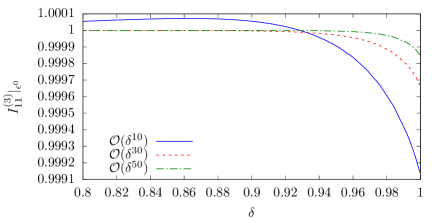
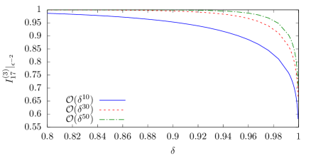
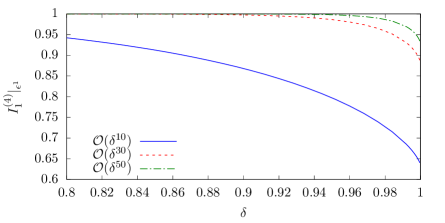
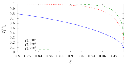
Figure 12: Comparison of exact and expanded phase-space master integrals for four typical examples, where the results are normalized to the exact expressions. The panel in the top row correspond to three-particle cut master integrals and the corresponding pictures can be found in Fig. 8. The pictures for the four-particle cut master integrals in the bottom row can found in Fig. 9. The considered $\epsilon$ order is indicated on the $y$-axis labels.

Following the approach described in the previous subsections we were able to obtain analytic results for all three- and four-particle cut master integrals, which are exact in $s$ and $m_{H}^{2}$. However, the expressions are quite large (in some cases of the order of several MB) and contain GPLs which have to be evaluated at some fixed value of their argument. We did not make any effort to obtain minimal expressions, since for our application it is sufficient to consider an expansion in the limit $\delta\to 0$. This can be obtained in a straightforward way by either expanding the exact results or by using the boundary conditions of Section 3.3 in combination with the differential equations.

In Fig. 12, for four typical examples of $\epsilon$ coefficients of master integrals, we compare the $\delta$-expanded and exact results. We normalize the curves to the exact expressions and plot the expansions as functions of $\delta$. In each panel three curves are shown, which correspond to approximations including 10, 30 and 50 terms of the $\delta$ expansion. All curves tend to 1 for $\delta\to 0$, so the plots focus on the region $0.8<\delta<1$ where the expansions start to diverge from the exact results.

The $\epsilon^{0}$ term of the three-particle cut integral $I^{(11)}$ (the first panel of Fig. 12) is an example for which as few as 10 $\delta$-expansion terms provide an excellent approximation. Even for $\delta=1$ the deviation from the exact result is at the level of 0.01%. Including additional expansion terms leads to further improvement. For the other three examples shown, we observe that the $\delta^{10}$ curves show deviations from the exact result at the percent level, even for $\delta$ values as small as 0.8. The approximations including expansion terms to order $\delta^{30}$ and $\delta^{50}$ show percent-level agreement with the exact results for $\delta$ values up to around 0.9 and 0.95, respectively.

In our final expression for the cross sections, we use the expansions up to $\delta^{30}$; from a practical point of view this is sufficient, since our large-$m_{t}$ approximation is only valid below the top threshold at $s=4m_{t}^{2}$. This corresponds to $\delta=1-4m_{H}^{2}/m_{t}^{2}\approx 0.48$, where the deviation of the expansions up to $\delta^{30}$ from the exact results is below $0.0001\%$ for all master integrals. On the other hand, the expansions up to $\delta^{10}$ show deviations of several percent.

4 Results

We are now in a position to combine the virtual, real-radiation and collinear counterterm corrections according to Eq. (3). It is interesting to check their contributions to the cancellation of the poles. In the $gg$ channel the highest-order poles, i.e. the $1/\epsilon^{4}$ and $1/\epsilon^{3}$ terms, receive contributions only from the virtual and real-radiation corrections. Starting from $1/\epsilon^{2}$ the collinear counterterm also contributes. In fact, there are two sources which can be identified from Eq. (12): either the term proportional to $1/\epsilon^{2}$ is convoluted with the LO cross section, or there are two convolutions of the one-loop splitting functions in the ${\cal O}(\alpha_{s})$ term, again with the LO cross section. The convolutions involving the two-loop splitting function and the convolutions of the one-loop splitting function with NLO partonic cross sections develop only $1/\epsilon$ poles.

For the partonic channels with quarks or anti-quarks in the initial state there are no virtual corrections. As a consequence the renormalized real-radiation contribution develops at most $1/\epsilon^{2}$ poles which cancel against those of the collinear counterterm contributions.

In the following we present analytic results for the renormalized partonic NNLO cross sections for all five channels. We restrict the expressions to the two leading terms in the $\delta$ expansion and we present only results up to order $1/m_{t}^{2}$ (or, $\rho^{1}$). To obtain compact expressions we set $\mu^{2}=m_{H}^{2}$. The top quark mass is renormalized in the on-shell scheme. In the supplementary material to this paper [62] we provide expansions for general renormalization scale $\mu$ up to $\delta^{30}$ and $1/m_{t}^{6}$ ($\rho^{3}$) (and for the quark-induced channels up to $1/m_{t}^{8}$ ($\rho^{4}$)) for both on-shell and $\overline{\rm MS}$ top quark masses. For the $gg$ channel our result is as follows:

$$\sigma_{gg}^{(2),n_{h}^{2}} =\frac{a_{s}^{4}G_{F}^{2}m_{H}^{2}}{\pi}\Bigg{\{}\delta^{3/2}\Bigg{(}\frac{19}{6912}+\frac{n_{l}}{1296}\Bigg{)}+\rho\Bigg{[}\sqrt{\delta}\Bigg{(}\frac{133}{552960}+\frac{7}{103680}n_{l}\Bigg{)}$$

$${}\vphantom{\Bigg{(}}+\delta^{3/2}\Bigg{(}\frac{613614937}{398131200}-\frac{695}{1492992}\log\rho-\frac{121217}{51840}\log 2+\frac{1964}{1215}\log^{2}(2)$$

$${}\vphantom{\Bigg{(}}-\frac{17129}{25920}\log^{3}(2)+\frac{7}{45}\log^{4}(2)-\frac{7753\pi^{2}}{103680}+\frac{18515\pi^{2}}{186624}\log 2-\frac{7\pi^{2}}{135}\log^{2}(2)$$

$${}\vphantom{\Bigg{(}}-\frac{931\pi^{4}}{829440}-\frac{171070393}{477757440}\zeta_{3}+\frac{1211}{2880}\zeta_{3}\log 2+\log\delta\Bigg{\{}-\frac{363953}{466560}+\frac{29009}{25920}\log 2$$

$${}\vphantom{\Bigg{(}}-\frac{12341}{17280}\log^{2}(2)+\frac{7}{30}\log^{3}(2)+\frac{3479\pi^{2}}{103680}-\frac{203\pi^{2}}{5760}\log 2+\frac{539}{3840}\zeta_{3}\Bigg{\}}$$

$${}\vphantom{\Bigg{(}}+\log^{2}(\delta)\Bigg{\{}\frac{29009}{155520}-\frac{1421}{5760}\log 2+\frac{91}{720}\log^{2}(2)-\frac{203\pi^{2}}{34560}\Bigg{\}}+\log^{3}(\delta)\Bigg{\{}-\frac{1421}{51840}$$

$${}\vphantom{\Bigg{(}}+\frac{7}{240}\log 2\Bigg{\}}+\frac{7}{2880}\log^{4}(\delta)+n_{l}\Bigg{\{}-\frac{1067831}{111974400}-\frac{533}{22394880}\log\rho$$

$${}\vphantom{\Bigg{(}}+\frac{50359}{3732480}\log 2-\frac{161}{19440}\log^{2}(2)+\frac{91}{38880}\log^{3}(2)+\frac{119\pi^{2}}{311040}-\frac{49\pi^{2}}{155520}\log 2$$

$${}\vphantom{\Bigg{(}}+\frac{371}{311040}\zeta_{3}+\log\delta\Bigg{[}\frac{1057}{233280}-\frac{49}{8640}\log 2+\frac{7}{2880}\log^{2}(2)-\frac{7\pi^{2}}{51840}\Bigg{]}$$

$${}\vphantom{\Bigg{(}}+\log^{2}(\delta)\Bigg{[}-\frac{49}{51840}+\frac{7}{8640}\log 2\Bigg{]}+\frac{7}{77760}\log^{3}(\delta)\Bigg{\}}\Bigg{)}\Bigg{]}+\mathcal{O}(\delta^{5/2})+\mathcal{O}(\rho^{2})\Bigg{\}}\,.$$ (47)

Note that the subset of the $n_{h}^{3}$ real-radiation terms with a closed top quark loop which has no coupling to Higgs bosons only contribute to higher-order $\delta$ terms not shown in Eq. (47). The $n_{h}^{4}$ terms (see Eq. (95) in Appendix D) are not included in this expression.

The result for the $gq$ channel is given by

$$\sigma_{gq}^{(2),n_{h}^{2}} =\frac{a_{s}^{4}G_{F}^{2}m_{H}^{2}}{\pi}\Bigg{\{}\rho\delta^{5/2}\Bigg{(}-\frac{259448903}{7873200000}+\frac{3096503}{65610000}\log 2-\frac{170443}{5832000}\log^{2}(2)$$

$$\vphantom{\Bigg{)}}+\frac{7777}{874800}\log^{3}(2)+\frac{553\pi^{2}}{432000}-\frac{1099\pi^{2}}{874800}\log 2+\frac{4151}{777600}\zeta_{3}+\log\delta\Bigg{[}\frac{8090963}{524880000}$$

$$\vphantom{\Bigg{)}}-\frac{346577}{17496000}\log 2+\frac{623}{64800}\log^{2}(2)-\frac{973\pi^{2}}{2332800}\Bigg{]}+\log^{2}(\delta)\Bigg{[}-\frac{227423}{69984000}$$

$$\vphantom{\Bigg{)}}+\frac{3871}{1166400}\log 2\Bigg{]}+\frac{2569}{6998400}\log^{3}(\delta)+n_{l}\Bigg{[}\frac{42287}{262440000}-\frac{973}{4374000}\log 2$$

$$\vphantom{\Bigg{)}}+\frac{49}{583200}\log^{2}(2){-\frac{7\pi^{2}}{6998400}}+\log\delta\Bigg{\{}-\frac{119}{2187000}+\frac{7}{194400}\log 2\Bigg{\}}$$

$$\vphantom{\Bigg{)}}+\frac{7}{2332800}\log^{2}(\delta)\Bigg{]}\Bigg{)}+\rho^{2}\Bigg{[}\delta^{3/2}\Bigg{(}-\frac{1446053}{755827200}+\frac{2829953}{1007769600}\log 2$$

$$\vphantom{\Bigg{)}}-\frac{207221}{111974400}\log^{2}(2)+\frac{54439}{83980800}\log^{3}(2)+\frac{18179\pi^{2}}{223948800}-\frac{7693\pi^{2}}{83980800}\log 2$$

$$\vphantom{\Bigg{)}}+\frac{29057}{74649600}\zeta_{3}+\log\delta\Bigg{\{}\frac{369229}{403107840}-\frac{16807}{13436928}\log 2+\frac{4361}{6220800}\log^{2}(2)$$

$$\vphantom{\Bigg{)}}-\frac{6811\pi^{2}}{223948800}\Bigg{\}}+\log^{2}(\delta)\Bigg{\{}-\frac{275233}{1343692800}+\frac{27097}{111974400}\log 2\Bigg{\}}+\frac{17983}{671846400}\log^{3}(\delta)$$

$$\vphantom{\Bigg{)}}+n_{l}\Bigg{\{}\frac{10241}{1007769600}-\frac{637}{41990400}\log 2+\frac{343}{55987200}\log^{2}(2)-\frac{49\pi^{2}}{671846400}$$

$$\vphantom{\Bigg{)}}+\log\delta\Bigg{[}-\frac{637}{167961600}+\frac{49}{18662400}{\log 2}\Bigg{]}+\frac{49}{223948800}\log^{2}(\delta)\Bigg{\}}\Bigg{)}$$

$$\vphantom{\Bigg{)}}+\delta^{5/2}\Bigg{(}-\frac{189454926667}{5290790400000}-\frac{10087}{279936000}\log\rho+\frac{8996488777}{176359680000}\log 2$$

$$\vphantom{\Bigg{)}}-\frac{1218467}{39191040}\log^{2}(2)+\frac{2780833}{293932800}\log^{3}(2)+\frac{5301953\pi^{2}}{3919104000}-\frac{392971\pi^{2}}{293932800}\log 2$$

$$\vphantom{\Bigg{)}}+\frac{1484279}{261273600}\zeta_{3}+\log\delta\Bigg{\{}\frac{5876601277}{352719360000}-\frac{2211991}{104976000}\log 2+\frac{222767}{21772800}\log^{2}(2)$$

$$\vphantom{\Bigg{)}}-\frac{347917\pi^{2}}{783820800}\Bigg{\}}+\log^{2}(\delta)\Bigg{\{}-\frac{40606843}{11757312000}+\frac{197737}{55987200}\log 2\Bigg{\}}$$

$$\vphantom{\Bigg{)}}+\frac{918601}{2351462400}\log^{3}(\delta)+n_{l}\Bigg{\{}\frac{1138687}{6298560000}-\frac{1435327}{5878656000}\log 2+\frac{2503}{27993600}\log^{2}(2)$$

$$\vphantom{\Bigg{)}}-\frac{2503\pi^{2}}{2351462400}+\log\delta\Bigg{[}-\frac{702131}{11757312000}+\frac{2503}{65318400}\log 2\Bigg{]}$$

$$\vphantom{\Bigg{)}}+\frac{2503}{783820800}\log^{2}(\delta)\Bigg{\}}\Bigg{)}\Bigg{]}+\mathcal{O}(\delta^{7/2})+\mathcal{O}(\rho^{3})\Bigg{\}}\,.$$ (48)

Here we display the $\rho\delta^{5/2}$, $\rho^{2}\delta^{3/2}$ and $\rho^{2}\delta^{5/2}$ terms. Note that the leading $\rho^{0}$ term starts at $\delta^{7/2}$ and so does not appear here. The channels $q\bar{q}$, $qq$ and $qq^{\prime}$ are further suppressed, as can be seen from their analytic expressions:

$$\sigma_{qq^{\prime}}^{(2),n_{h}^{2}} =\frac{a_{s}^{4}G_{F}^{2}m_{H}^{2}}{\pi}\Bigg{\{}\rho\delta^{7/2}\Bigg{(}\frac{565457}{1607445000}-\frac{599}{1275750}\log 2+\frac{\log^{2}(2)}{4050}-\frac{\pi^{2}}{72900}$$

$$\vphantom{\Bigg{)}}+\log\delta\Bigg{[}-\frac{599}{3827250}+\frac{\log 2}{6075}\Bigg{]}+\frac{\log^{2}(\delta)}{36450}\Bigg{)}+\rho^{2}\Bigg{[}\delta^{5/2}\Bigg{(}\frac{493577}{15746400000}$$

$$\vphantom{\Bigg{)}}-\frac{3773}{87480000}\log 2+\frac{49}{1944000}\log^{2}(2)-\frac{49\pi^{2}}{34992000}+\log\delta\Bigg{\{}-\frac{3773}{262440000}$$

$$\vphantom{\Bigg{)}}+\frac{49}{2916000}\log 2\Bigg{\}}+\frac{49}{17496000}\log^{2}(\delta)\Bigg{)}+\delta^{7/2}\Bigg{(}\frac{344611787}{840157920000}-\frac{181147}{333396000}\log 2$$

$$\vphantom{\Bigg{)}}+\frac{1783}{6350400}\log^{2}(2)-\frac{1783\pi^{2}}{114307200}+\log\delta\Bigg{[}-\frac{181147}{1000188000}+\frac{1783}{9525600}\log 2\Bigg{]}$$

$$\vphantom{\Bigg{)}}+\frac{1783}{{57153600}}\log^{2}(\delta)\Bigg{)}\Bigg{]}+\mathcal{O}(\delta^{9/2})+\mathcal{O}(\rho^{3})\Bigg{\}}\,,$$ (49)

$$\vphantom{\Bigg{)}}\Delta^{(2),n_{h}^{2}}_{qq} ={\frac{a_{s}^{4}G_{F}^{2}m_{H}^{2}}{\pi}\Bigg{\{}}-\frac{7}{104976000}\rho^{2}\delta^{7/2}+\mathcal{O}(\delta^{9/2})+\mathcal{O}(\rho^{3})\Bigg{\}}\,,$$ (50)

$$\vphantom{\Bigg{)}}\Delta^{(2),n_{h}^{2}}_{q\overline{q}} ={\frac{a_{s}^{4}G_{F}^{2}m_{H}^{2}}{\pi}\Bigg{\{}}\frac{31}{1020600}\rho^{2}\delta^{7/2}+\mathcal{O}(\delta^{9/2})+\mathcal{O}(\rho^{3})\Bigg{\}}\,,$$ (51)

where $\sigma_{xy}=\Delta_{xy}+\sigma_{qq^{\prime}}$.

In the ancillary files [62] we provide the renormalized cross sections with tags for the virtual, real-radiation and collinear counterterm contributions, which allows one to extract the individual contributions if desired. This means that these expressions contain poles in $\epsilon$, which cancel upon removing the tags.

In Fig. 13 we plot the partonic cross section for all five channels as a function of $\sqrt{s}$, with the renormalization scale $\mu^{2}=m_{H}^{2}$. We combine all corrections, including the $n_{h}^{3}$ terms from Ref. [25], the $n_{h}^{4}$ terms from Appendix D and the $q\bar{q}\to HH$ virtual corrections from Appendix C.

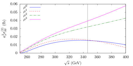
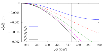
(a)	(b)
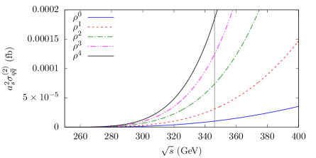
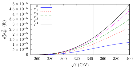
(c)	(d)
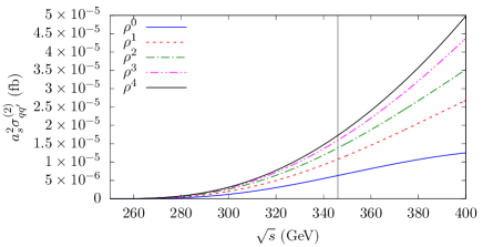
(e)

Figure 13: The five NNLO partonic contributions as a function of $\sqrt{s}$, with the renormalization scale $\mu^{2}=m_{H}^{2}$. The colours and line styles denote the inclusion of higher orders in the $\rho=m_{H}^{2}/m_{t}^{2}$ expansion. Note that the cross sections have been multiplied by two powers of $a_{s}=\alpha_{s}^{(5)}/\pi$. The vertical black line indicates the top quark threshold at $\sqrt{s}=2m_{t}$.

The overall picture is similar to the LO, NLO and NNLO $n_{h}^{3}$ contributions [9, 25]; a reasonable convergence pattern is observed for $\sqrt{s}\;\hbox to0.0pt{\lower 3.5pt\hbox{$\mathchar 0\relax\sim$}\hss}\raise 1.0pt\hbox{$<$}\;320$ GeV, which rapidly deteriorates for values of $\sqrt{s}$ above the top quark threshold. For the $qg$, $qq$ and $qq^{\prime}$ channels one observes a better convergence behaviour than for the $gg$ channel. Similar to NLO, the $q\bar{q}$ channel shows the worst behaviour. Note that there is a strong hierarchy in the numerical size of the various contributions, ranging from ${\cal O}(10^{-2})$ fb for the $gg$ channel to ${\cal O}(10^{-5})$ fb for the $qq$ and $qq^{\prime}$ channels.

By construction all curves have to approach zero in a continuous way for $\sqrt{s}\to 2m_{H}$. This is clearly visible from the plots for all channels with quarks in the initial state, however for the $gg$ channel the plot gives the impression that this is not the case for the $\rho^{2}$ and $\rho^{3}$ curves. Inspecting the analytic result reveals that there are terms containing $\rho^{2}\sqrt{\delta}\log^{4}(\delta)$ and $\rho^{3}\sqrt{\delta}\log^{4}(\delta)$ which are responsible for a rapid rise in the cross section close to the threshold.

Although the radius of convergence of the large-$m_{t}$ expansion is quite limited here, it contains useful information for the construction of approximated NNLO results. For example, in Ref. [14] NLO virtual corrections to double Higgs boson production are considered. The analytic structure of the form factors close to the top quark threshold is combined with results obtained in the large-$m_{t}$ limit. Stable approximations are only obtained after including power-suppressed $1/m_{t}$ terms. This approach has been applied in Refs. [65, 66] to the Higgs-gluon form factor and also there it was found that it is important to include higher-order $1/m_{t}$ terms to obtain a stable result in the high-energy region.

5 Conclusions

The main achievement of this paper is the computation of the NNLO real-radiation contribution to the total cross section of the process $gg\to HH$ in an expansion for large top quark mass. This improves the description beyond the infinite top quark mass limit and provides important information for NNLO approximation procedures.

We provide a detailed description of the various steps of our calculation and in particular discuss the computation of the three- and four-particle phase-space master integrals. We provide various intermediate results which might be useful for other calculations. In the ancillary files of this paper we provide separate results for the virtual corrections, real-radiation contribution and the collinear counterterm.

The inclusion of the power-suppressed terms significantly increases the cross section below the top quark threshold. For example, at NNLO, for a partonic center-of-mass energy $\sqrt{s}\approx 300$ GeV the cross section increases almost by a factor of two after including the $1/m_{t}^{4}$ and $1/m_{t}^{6}$ terms.

Appendix

Appendix A Auxiliary formulae for the collinear counterterm

In this appendix we provide some details on the analytic computation of the convolution integrals in an expansion in $\delta$.

All integrals contributing to Eq. (10) have the form

$$\int^{1}_{1-\delta}\mathrm{d}z\>Q(z)\sigma_{X}(x/z)\,,$$ (52)

where $Q(z)$ is either a single splitting function or the convolution of two splitting functions and $\sigma_{X}$ is one of the following LO or NLO cross sections,

$$\sigma_{X}\in\left\{\sigma_{gg}^{(0)},\quad\sigma_{gg}^{(1)},\quad\sigma_{gq}^{(1)},\quad\sigma_{q\bar{q}}^{(1)}\right\}\,.$$ (53)

These are renormalized finite quantities which we need up to ${\cal O}(\epsilon^{2})$ at LO and ${\cal O}(\epsilon)$ at NLO.

We introduce the variables

$$x=\frac{m_{H}^{2}}{s},\quad\delta=1-4x,\quad z=\frac{1-\delta}{1-\delta\nu}\,,$$ (54)

and obtain

$$\int^{1}_{1-\delta}\mathrm{d}z=\int^{1}_{0}\frac{\delta(1-\delta)}{(1-\delta\nu)^{2}}\mathrm{d}\nu\,,$$ (55)

and

$$\frac{x}{z}=\frac{1-\delta\nu}{4}\,.$$ (56)

This allows us to rewrite Eq. (52) as

$$\int^{1}_{1-\delta}\mathrm{d}z\>Q(z)\sigma_{X}(x/z)=\int^{1}_{0}\mathrm{d}\nu\>Q\!\left(\frac{1-\delta}{1-\delta\nu}\right)\frac{\delta(1-\delta)}{(1-\delta\nu)^{2}}\sigma_{X}\left({\frac{1-\delta\nu}{4}}\right)\,,$$ (57)

where $Q(z)$ can be rational functions of $z$, a plus distribution or a delta function. It may also contain logarithms or dilogarithms. In the latter case it is convenient to rewrite the arguments using the identities

$$\mathrm{Li}_{2}(-z) =\frac{1}{2}\mathrm{Li}_{2}(z^{2})-\mathrm{Li}_{2}(z)\,,$$

$$\mathrm{Li}_{2}(z) =-\mathrm{Li}_{2}(1-z)-\log(z)\log(1-z)+\frac{\pi^{2}}{6}\,,$$

$$\mathrm{Li}_{2}(z^{2}) =-\mathrm{Li}_{2}(1-z^{2})-2\log(z)\log(1-z)-2\log(z)\log(1+z)+\frac{\pi^{2}}{6}\,.$$ (58)

In this way, we obtain $Q(z)$ in terms of $\mathrm{Li}_{2}(1-z)$ and $\mathrm{Li}_{2}(1-z^{2})$ and the expansion around $\delta=0$, which corresponds to $z=1$, is straightforward.

A.1 $\sigma_{gg}^{(0)}$

Let us first consider the contributions involving the LO cross section which has a simple series expansion in $\delta$

$$\sigma_{gg}^{(0)}(x)\Big{|}_{x=\frac{1-\delta}{4}}=\sum_{n=0}^{\infty}\delta^{\frac{1}{2}+n-\epsilon}\sum_{u=0}^{N_{\epsilon}^{\mathrm{max}}}\epsilon^{u}c^{(n,u),(0)}_{gg}\,,$$ (59)

where for our application we have $N_{\epsilon}^{\mathrm{max}}=2$. Note the the coefficients $c^{(n,u),(0)}_{gg}$ are available from an explicit calculation of $\sigma_{gg}^{(0)}(x)$. In the following we discuss the various cases for $Q(z)$ which appear.

For the case of $Q(z)=z^{r}$, where in our case only $r\geq-1$ is needed, we have

$$\int^{1}_{1-\delta}\mathrm{d}z~{}\sigma_{gg}^{(0)}(x/z)~{}z^{r} =\sum_{n=0}^{\infty}\delta^{3/2+n}(1-\delta)^{r+1}\sum_{j=0}^{n}\sum_{u=0}^{N_{\epsilon}^{\mathrm{max}}}\frac{(n-j+r+1)!}{(r+1)!(n-j)!}\frac{\delta^{-\epsilon}}{\frac{3}{2}+n-\epsilon}c^{(j,u),(0)}_{gg}\epsilon^{u}\,,$$ (60)

and for $Q(z)=1/(1+z)$,

$$\int^{1}_{1-\delta}\mathrm{d}z~{}\frac{\sigma_{gg}^{(0)}(x/z)}{1+z}=$$

$$\qquad\sum_{n=0}^{\infty}\delta^{\frac{3}{2}+n}(1-\delta)\sum_{k=0}^{n}\sum_{j=0}^{k}\sum_{s=0}^{n-k}\sum_{u=0}^{N_{\epsilon}^{\mathrm{max}}}\frac{1}{2^{n-k+1}}\frac{(n-k)!}{s!(n-k-s)!}\frac{\delta^{-\epsilon}}{\frac{3}{2}+k+s-\epsilon}c^{(j,u),(0)}_{gg}\epsilon^{u}\,.$$ (61)

These formulae are obtained with the help of Eqs. (54) and (55) which are used to replace $z$ by $\nu$. Afterwards we insert Eq. (59), expand in $\delta$ and integrate each term individually. This approach is also used for the results which we present below. Due to the more complicated functions $Q(z)$ some of the formulae are more involved. Although the formulae we present are exact, we apply an upper limit to the $\delta$ expansion when we use them in our calculations.

Now we consider $Q(z)=\left[\frac{(\log(1-z))^{r}}{1-z}\right]_{+}$. Using the definition of the plus distribution we obtain

$$\int^{1}_{1-\delta}\mathrm{d}z\left[\frac{(\log(1-z))^{r}}{1-z}\right]_{+}\sigma_{gg}^{(0)}(x/z)=$$

$$\qquad\int^{1}_{1-\delta}\mathrm{d}z\frac{(\log(1-z))^{r}}{1-z}\left(\sigma_{gg}^{(0)}\left(\frac{x}{z}\right)-\sigma_{gg}^{(0)}(x)\right)+\frac{(\log\delta)^{r+1}}{r+1}\sigma_{gg}^{(0)}(x)\,.$$ (62)

In order to compute the finite integral on the r.h.s., we consider $Q(z)=(1-z)^{-1+\eta}$ which leads to

$$\int^{1}_{1-\delta}\mathrm{d}z~{}\sigma_{gg}^{(0)}(x/z)~{}(1-z)^{-1+\eta}=$$

$$\qquad\sum_{l=0}^{\infty}\sum_{m=0}^{\infty}\sum_{u=0}^{N_{\epsilon}^{\mathrm{max}}}\frac{\Gamma(1+\eta+l)}{\Gamma(1+\eta)l!}\delta^{\frac{1}{2}+m+l+\eta-\epsilon}(1-\delta)\epsilon^{u}c^{(m,u),(0)}_{gg}\frac{\Gamma(\eta)\Gamma(\frac{3}{2}+m+l-\epsilon)}{\Gamma(\frac{3}{2}+m+l+\eta-\epsilon)}\,.$$ (63)

Note that this formula is exact in $\eta$. Using $\sigma_{gg}^{(0)}(x)$ instead of $\sigma_{gg}^{(0)}(x/z)$ we have

$$\int^{1}_{1-\delta}\mathrm{d}z~{}\sigma_{gg}^{(0)}(x)~{}(1-z)^{-1+\eta}=$$

$$\qquad\sum_{l=0}^{\infty}\sum_{m=0}^{\infty}\sum_{u=0}^{N_{\epsilon}^{\mathrm{max}}}\frac{\Gamma(1+\eta+l)}{\Gamma(1+\eta)l!}\delta^{\frac{1}{2}+m+l+\eta-\epsilon}(1-\delta)\epsilon^{u}c^{(m,u),(0)}_{gg}\frac{\Gamma(\eta)\Gamma(1+l)}{\Gamma(1+l+\eta)}\,.$$ (64)

After combining both expressions we obtain

$$\int^{1}_{1-\delta}\mathrm{d}z~{}(1-z)^{-1+\eta}\left[\sigma_{gg}^{(0)}\left(\frac{x}{z}\right)-\sigma_{gg}^{(0)}(x)\right]=\sum_{n=0}^{\infty}\delta^{\frac{1}{2}+n-\epsilon}(1-\delta)\sum_{j=0}^{n}\sum_{u=0}^{N_{\epsilon}^{\mathrm{max}}}\epsilon^{u}c^{(j,u),(0)}_{gg}$$

$$\mbox{}\qquad\left[\Psi_{j,n}+\eta\left((\log\delta+\psi(n-j+1))\Psi_{j,n}+\frac{\Psi^{(1)}_{j,n}-\Psi^{(2)}_{j,n}}{2}\right)+\mathcal{O}(\eta^{2})\right]\,,$$ (65)

where

$$\Psi_{j,n} =\psi\left(n-j+1\right)-\psi\left(\frac{3}{2}+n-\epsilon\right)\,,$$

$$\Psi^{(1)}_{j,n} =\psi^{\prime}\left(n-j+1\right)-\psi^{\prime}\left(\frac{3}{2}+n-\epsilon\right)\,,$$

$$\Psi^{(2)}_{j,n} =\left[\psi\left(n-j+1\right)\right]^{2}-\left[\psi\left(\frac{3}{2}+n-\epsilon\right)\right]^{2}\,.$$ (66)

Here $\psi(x)$ is the polygamma function and $\psi^{\prime}(x)\equiv\psi^{(1)}$ its derivative. The results for Eq. (62) are obtained by expanding the l.h.s. of Eq. (65) in $\eta$ according to

$$(1-z)^{-1+\eta}=\frac{1}{1-z}\left[1+\eta\log(1-z)+\frac{\eta^{2}}{2}\left(\log(1-z)\right)^{2}+\cdots\right]\,.$$ (67)

Note that the r.h.s of Eq. (65) is already expanded in $\eta$. The comparison of the $\eta^{0}$ and $\eta^{1}$ terms provides results for Eq. (62) for $r=0$ and $r=1$, which we need for our calculations.

Next we treat cases such as

$$Q(z)=\frac{\log(z)\log(1-z)}{1-z},\quad Q(z)=z^{2}\log(1-z),\ldots\,,$$ (68)

i.e., $Q(z)$ contains factors of $z$ and $1-z$ with positive or negative exponents, and/or logarithms with $z$ or $1-z$ as argument. Here it is convenient first to consider

$$Q(z)=z^{r_{1}}(1-z)^{r_{2}}\,,$$ (69)

with non-integer exponents $r_{1}$ and $r_{2}$. The resulting formula can then be expanded around $r_{1},r_{2}=-1,0,\ldots$ in order to obtain the result for the desired $Q(z)$ of Eq. (68). The generic result for $Q(z)$ from Eq. (69) is given by

$$\int^{1}_{1-\delta}\mathrm{d}z~{}\sigma_{gg}^{(0)}(x/z)~{}z^{r_{1}}(1-z)^{r_{2}}=\sum_{n=0}^{\infty}\delta^{\frac{3}{2}+n-\epsilon+r_{2}}(1-\delta)^{1+r_{1}}$$

$$\qquad\sum_{j=0}^{n}\sum_{u=0}^{N_{\epsilon}^{\mathrm{max}}}\frac{\Gamma(r_{1}+r_{2}+2+n-j)\Gamma(r_{2}+1)\Gamma(\frac{3}{2}+n-\epsilon)}{\Gamma(r_{1}+r_{2}+2)\Gamma(\frac{5}{2}+n-\epsilon+r_{2})(n-j)!}\epsilon^{u}c^{(j,u),(0)}_{gg}\,.$$ (70)

To obtain the result for $Q(z)=z^{2}\log(1-z)$ we set $r_{1}=2$ and $r_{2}=\eta$. Afterwards we expand Eq. (70) in $\eta$ and take the coefficient of the linear term, on both sides. In a similar way one can treat $Q(z)=\log(z)$ by setting $r_{1}=\eta$ and $r_{2}=0$.

In case $Q(z)$ (from Eq. (68)) contains a $\log(z)$ term a non-integer value for $r_{1}$ must be chosen.

Cases such as

$$Q(z)=\frac{\log(z)\log(1+z)}{1+z},\quad z^{2}\log(1+z),\ldots$$ (71)

can be treated in a similar way. Here a convenient auxiliary function is given by

$$Q(z)=z^{r_{1}}(1+z)^{r_{2}}\,,$$ (72)

where the desired result is again obtained by a suitable choice of $r_{1}$ and $r_{2}$ supplemented by proper expansions. The generic integral is given by

$$\int^{1}_{1-\delta}\mathrm{d}z~{}\sigma_{gg}^{(0)}(x/z)~{}z^{r_{1}}(1+z)^{r_{2}}=\sum_{n=0}^{\infty}\sum_{k=0}^{n}\sum_{j=0}^{k}\sum_{s=0}^{n-k}\sum_{u=0}^{N_{\epsilon}^{\mathrm{max}}}{2^{r_{2}-n+k}}\delta^{\frac{3}{2}+n-\epsilon}(1-\delta)^{1+r_{1}}$$

$$\qquad\frac{\Gamma(-r_{2}+n-k)\Gamma(r_{1}+r_{2}+2+k-j)}{\Gamma(-r_{2})(n-k-s)!s!\Gamma(r_{1}+r_{2}+{2})(k-j)!}\epsilon^{u}c^{(j,u),(0)}_{gg}\frac{1}{\frac{3}{2}+k+s-\epsilon}\,.$$ (73)

Note that the expression on the r.h.s. is significantly more complex than Eq. (70). This is due to the fact that the factor $(1+z)^{r_{2}}$ introduces a new type of denominator whereas $(1-z)\sim\delta$ and thus no new structure is introduced.

Having dealt with logarithms, we now turn to functions $Q(z)$ which involve dilogarithms. For $Q(z)=z^{r}\mathrm{Li}_{2}(1-z)$ we have

$$\int^{1}_{1-\delta}\mathrm{d}z~{}z^{r}\mathrm{Li}_{2}(1-z)~{}\sigma_{gg}^{(0)}(x/z)=\sum_{n=1}^{\infty}\delta^{\frac{3}{2}+n-\epsilon}(1-\delta)^{1+r}$$

$$\qquad\sum_{k=0}^{n-1}\sum_{j=0}^{k}\sum_{u=0}^{N_{\epsilon}^{\mathrm{max}}}\frac{1}{(n-k)^{2}}\frac{(r+n-j+1)!}{(r+n-k+1)!(k-j)!}\frac{\Gamma(n-k+1)\Gamma(\frac{3}{2}+k-\epsilon)}{\Gamma(\frac{5}{2}+n-\epsilon)}\epsilon^{u}c^{(j,u),(0)}_{gg}\,,$$ (74)

and for $Q(z)=\mathrm{Li}_{2}(1-z)/(1-z)$ the corresponding integral has the form

$$\int^{1}_{1-\delta}\mathrm{d}z~{}\frac{\mathrm{Li}_{2}(1-z)}{1-z}~{}\sigma_{gg}^{(0)}(x/z)=$$

$$\qquad\sum_{n=1}^{\infty}\delta^{\frac{1}{2}+n-\epsilon}(1-\delta)\sum_{k=0}^{n-1}\sum_{j=0}^{k}\sum_{u=0}^{N_{\epsilon}^{\mathrm{max}}}\frac{(n-j)!\Gamma(\frac{3}{2}+k-\epsilon)}{(n-k)^{3}(k-j)!\Gamma(\frac{3}{2}+n-\epsilon)}\epsilon^{u}c^{(j,u),(0)}_{gg}\,.$$ (75)

For $Q(z)=\mathrm{Li}_{2}(1-z)/(1+z)$ we have

$$\int^{1}_{1-\delta}\mathrm{d}z~{}\frac{\mathrm{Li}_{2}(1-z)}{1+z}~{}\sigma_{gg}^{(0)}(x/z)=\sum_{n=1}^{\infty}\delta^{\frac{3}{2}+n-\epsilon}(1-\delta)\sum_{h=0}^{n-1}\sum_{k=0}^{h}\sum_{j=0}^{k}\sum_{w=0}^{h-k}\sum_{u=0}^{N_{\epsilon}^{\mathrm{max}}}\frac{\epsilon^{u}c^{(j,u),(0)}_{gg}}{2^{h-k+1}}$$

$$\qquad\frac{(h-k)!(n-h+k-j)!}{(h-k-w)!w!(k-j)!(n-h)^{2}}\frac{\Gamma(\frac{3}{2}+k+w-\epsilon)}{\Gamma(\frac{5}{2}+n-h+k+w-\epsilon)}\,,$$ (76)

and for $Q(z)=z^{r}\mathrm{Li}_{2}(1-z^{2})$ the integral is given by

$$\int^{1}_{1-\delta}\mathrm{d}z~{}z^{r}\mathrm{Li}_{2}(1-z^{2})~{}\sigma_{gg}^{(0)}(x/z)=\sum_{n=1}^{\infty}\delta^{\frac{3}{2}+n-\epsilon}(1-\delta)^{1+r}\sum_{k=0}^{n-1}\sum_{j=0}^{k}\sum_{w=0}^{[\frac{n-k}{2}]}\sum_{h=0}^{w}\sum_{u=0}^{N_{\epsilon}^{\mathrm{max}}}\epsilon^{u}c^{(j,u),(0)}_{gg}$$

$$\qquad\frac{(-1)^{w}((n-k-w)!)^{2}(r+2n-k-j-2w+1)!2^{n-k-2w}}{(n-k-w)^{2}(n-k-2w)!(w-h)!h!(r+2n-2k-2w+1)!(k-j)!}\times$$

$$\qquad\frac{\Gamma(\frac{3}{2}+k+h-\epsilon)}{\Gamma(\frac{5}{2}+n+h-w-\epsilon)}\,.$$ (77)

Finally, for $Q(z)=\mathrm{Li}_{2}(1-z^{2})/(1+z)$ we have

$$\int^{1}_{1-\delta}\mathrm{d}z~{}\frac{1}{1+z}\mathrm{Li}_{2}(1-z^{2})~{}\sigma_{gg}^{(0)}(x/z)=\sum_{n=1}^{\infty}\delta^{\frac{3}{2}+n-\epsilon}(1-\delta)\sum_{k=0}^{n-1}\sum_{j=0}^{k}\sum_{w=0}^{[\frac{n-k-1}{2}]}\sum_{h=0}^{w}\sum_{u=0}^{N_{\epsilon}^{\mathrm{max}}}\epsilon^{u}c^{(j,u),(0)}_{gg}$$

$$\qquad\frac{(-1)^{w}((n-k-w-1)!)^{2}(2n-k-j-2w)!2^{n-k-2w-1}}{(n-k-w)(n-k-2w-1)!(w-h)!h!(2n-2k-2w)!(k-j)!}\times$$

$$\qquad\frac{\Gamma(\frac{3}{2}+k+h-\epsilon)}{\Gamma(\frac{5}{2}+n+h-w-\epsilon)}\,.$$ (78)

A.2 $\sigma_{gg}^{(1)},\sigma_{gq}^{(1)},\sigma_{q\bar{q}}^{(1)}$

In this subsection we consider the NLO partonic cross sections $\sigma_{gg}^{(1)},\sigma_{gq}^{(1)}$ and $\sigma_{q\bar{q}}^{(1)}$ which have the following expansion in $\delta$

$$\sigma_{X}(x)\Big{|}_{x=\frac{1-\delta}{4}}=\sum_{n=0}^{\infty}\delta^{\frac{1}{2}+n}\sum_{u=0}^{N_{\epsilon}^{\mathrm{max}}}\sum_{v=0}^{u+2}\epsilon^{u}(\log\delta)^{v}c^{(n,u,v)}_{X}\,,$$ (79)

with known coefficients $c^{(n,u,v)}_{X}$. For our application $N_{\epsilon}^{\mathrm{max}}=1$ is sufficient. Note the explicit presence of $\log\delta$ terms which cannot be factorized as at LO in Eq. (59). With the help of Eq. (56) we also introduce

$$\sigma_{X}(x/z)\Big{|}_{x=\frac{1-\delta}{4}}=\sum_{n=0}^{\infty}(\delta\nu)^{\frac{1}{2}+n}\sum_{u=0}^{N_{\epsilon}^{\mathrm{max}}}\sum_{v=0}^{u+2}\epsilon^{u}(\log\nu)^{v}\tilde{c}^{(n,u,v)}_{X}\,,$$ (80)

where the coefficients $\tilde{c}^{(n,u,v)}_{X}$ are functions of $\log\delta$, which for the relevant values of $u$ and $v$ are given in terms of $c^{(n,u,v)}_{X}$ by:

$$\tilde{c}^{(n,0,0)}_{X} =c^{(n,0,0)}_{X}+c^{(n,0,1)}_{X}\log\delta+c^{(n,0,2)}_{X}(\log\delta)^{2}\,,$$

$$\tilde{c}^{(n,0,1)}_{X} =c^{(n,0,1)}_{X}+2c^{(n,0,2)}_{X}\log\delta\,,$$

$$\tilde{c}^{(n,0,2)}_{X} =c^{(n,0,2)}_{X}\,,$$

$$\tilde{c}^{(n,1,0)}_{X} =c^{(n,1,0)}_{X}+c^{(n,1,1)}_{X}\log\delta+c^{(n,1,2)}_{X}(\log\delta)^{2}+c^{(n,1,3)}_{X}(\log\delta)^{3}\,,$$

$$\tilde{c}^{(n,1,1)}_{X} =c^{(n,1,1)}_{X}+2c^{(n,1,2)}_{X}\log\delta+3c^{(n,1,3)}_{X}(\log\delta)^{2}\,,$$

$$\tilde{c}^{(n,1,2)}_{X} =c^{(n,1,2)}_{X}+3c^{(n,1,3)}_{X}\log\delta\,,$$

$$\tilde{c}^{(n,1,3)}_{X} =c^{(n,1,3)}_{X}\,.$$ (81)

Note that the coefficients in Eq. (81) can be used to write Eq. (79) in the form

$$\sigma_{X}(x)\Big{|}_{x=\frac{1-\delta}{4}}=\sum_{n=0}^{\infty}\delta^{\frac{1}{2}+n}\sum_{u=0}^{N_{\epsilon}^{\mathrm{max}}}\epsilon^{u}\tilde{c}^{(n,u,0)}_{X}\,.$$ (82)

We are now in the position to insert the relevant expressions for $Q(z)$ in Eq. (57) and perform an expansion in $\delta$. The NLO cross sections are only convoluted with one-loop splitting functions which leaves us with $Q(z)=z^{r}$ and $Q(z)=\left[\frac{1}{1-z}\right]_{+}$. For $Q(z)=z^{r}$ we have

$$\int^{1}_{1-\delta}\mathrm{d}z~{}\sigma_{X}(x/z)~{}z^{r}=$$

$$\qquad(1-\delta)^{r+1}\sum_{n=0}^{\infty}\delta^{\frac{3}{2}+n}\sum_{j=0}^{n}\frac{(r+n-j+1)!}{(r+1)!(n-j)!}\sum_{u=0}^{N_{\epsilon}^{\mathrm{max}}}\sum_{v=0}^{u+2}\epsilon^{u}\tilde{c}^{(j,u,v)}_{X}\frac{(-1)^{v}v!}{(3/2+n)^{v+1}}\,.$$ (83)

For $Q(z)=\left[\frac{1}{1-z}\right]_{+}$ we use Eq. (62) for $r=0$ and obtain for the integral on the r.h.s.

$$\int^{1}_{1-\delta}\mathrm{d}z\frac{1}{1-z}\left(\sigma_{X}\left(\frac{x}{z}\right)-\sigma_{X}(x)\right)=(1-\delta)\times$$

$$\qquad\sum_{n=0}^{\infty}\sum_{j=0}^{n}\delta^{\frac{1}{2}+n}\sum_{u=0}^{N_{\epsilon}^{\mathrm{max}}}\epsilon^{u}\left[\psi(n-j+1)\tilde{c}^{(j,u,0)}_{X}-\sum_{v={0}}^{u+2}\psi^{(v)}\!\left(\!\frac{3}{2}+n\!\right)\tilde{c}^{(j,u,v)}_{X}\right].$$ (84)

For $N_{\epsilon}^{\mathrm{max}}=1$, terms with up to three derivatives of the polygamma function appear on the r.h.s. of Eq. (84).

Appendix B Cross-check from $gg\to H$

In this appendix we describe how the leading terms in the $1/m_{t}$ expansion (i.e. the $m_{t}^{0}$ terms) of the Higgs pair cross section can be cross-checked using known results from single-Higgs boson production. The approach described below can be used to cross-check the divergent building blocks entering the individual channels.

At leading order in $1/m_{t}$ the Higgs-pair cross section is obtained by interpreting the Higgs boson mass in the single-Higgs cross section as the invariant mass of the Higgs boson pair, $m_{HH}$, and subsequently integrating over $m_{HH}$ (see also Ref. [28]). Our master formula reads

$$\sigma_{HH}^{[x]}=\int^{\sqrt{s}}_{2m_{H}}{\rm d}m_{HH}\frac{d\sigma^{\mathrm{[x]}}_{HH}}{dm_{HH}} =\int^{\sqrt{s}}_{2m_{H}}{\rm d}m_{HH}f^{\epsilon}_{H\to HH}\left(\frac{C_{HH}}{C_{H}}-\frac{6\lambda v^{2}}{m_{HH}^{2}-m_{H}^{2}}\right)^{2}\sigma^{\mathrm{[x]}}_{H}\Big{|}_{m_{H}\to m_{HH}}\,,$$ (85)

where the superscript “[x]” of $\sigma^{\mathrm{[x]}}_{HH}$ and $\sigma^{\mathrm{[x]}}_{H}$ represent the (divergent) individual pieces. For example, $\sigma^{\mathrm{[rr]}}_{HH}$ denotes the real-real and $\sigma^{\mathrm{[coll]}}_{HH}$ the collinear counterterm contribution. In Eq. (85) the function $f^{\epsilon}_{H\to HH}$ takes into account the $d$-dimensional two-particle phase space and is given by

$$f^{\epsilon}_{H\to HH}=e^{\epsilon\gamma_{E}}\frac{\Gamma(1-\epsilon)}{\Gamma(2-2\epsilon)}\frac{(m_{HH}^{2}-4m_{H}^{2})^{1/2-\epsilon}}{16\pi^{2}v^{2}}\left(\frac{\mu^{2}}{m_{H}^{2}}\right)^{\epsilon}\,.$$ (86)

The ratio of the matching coefficients $C_{HH}$ and $C_{H}$, including higher order terms in $\epsilon$, reads [32]

$$\frac{C_{HH}}{C_{H}}= 1+2\epsilon+\frac{\alpha_{s}^{(5)}(\mu)}{\pi}\left[\frac{3\epsilon}{2}+\left(\frac{3}{2}\log\frac{\mu^{2}}{m_{t}^{2}}-\frac{11}{3}\right)\epsilon^{2}\right]+\left(\frac{\alpha_{s}^{(5)}(\mu)}{\pi}\right)^{2}\Bigg{\{}\frac{19}{8}-\frac{11n_{h}}{12}+\frac{2n_{l}}{3}$$

$$\qquad+\epsilon\left[-\frac{95}{16}+\frac{91n_{h}}{144}-\frac{13n_{l}}{8}+\log\frac{\mu^{2}}{m_{t}^{2}}\left(\frac{71}{8}-\frac{11n_{h}}{6}+\frac{13n_{l}}{12}\right)\right]\Bigg{\}}\,,$$ (87)

where $m_{t}\equiv m_{t}(\mu)$ is the top quark mass renormalized in the $\overline{\rm MS}$ scheme.

Our aim is to compute the integral in Eq. (85) in an expansion in $\delta$. To do so it is convenient to use the following change of variable,

$$m_{HH}^{2}=\frac{4m_{H}^{2}(1-\delta\nu)}{1-\delta}\,.$$ (88)

This allows us to rewrite $f^{\epsilon}_{H\to HH}$ as

$$f^{\epsilon}_{H\to HH}=e^{\epsilon\gamma_{E}}\frac{\Gamma(1-\epsilon)}{\Gamma(2-2\epsilon)}\frac{(4\delta)^{1/2-\epsilon}\>(1-\delta)^{-1/2+\epsilon}\>(1-\nu)^{1/2-\epsilon}}{16\pi^{2}v^{2}}\left(\frac{\mu^{2}}{m_{H}^{2}}\right)^{\epsilon}$$ (89)

and the integral in Eq. (85) is then written as

$$\int^{\sqrt{s}}_{2m_{H}}{\rm d}m_{HH}f^{\epsilon}_{H\to HH}\left(\frac{C_{HH}}{C_{H}}-\frac{6\lambda v^{2}}{m_{HH}^{2}-m_{H}^{2}}\right)^{2}\sigma^{\mathrm{[x]}}_{H}\Big{|}_{m_{H}\to m_{HH}}=$$

$$\qquad\int^{1}_{0}{\rm d}\nu\frac{2m_{H}\delta}{\sqrt{1-\delta}\sqrt{1-\delta\nu}}f^{\epsilon}_{H\to HH}\left(\frac{C_{HH}}{C_{H}}-\frac{6\lambda v^{2}(\delta-1)}{m_{H}^{2}(-3-\delta+4\delta\nu)}\right)^{2}\sigma^{\mathrm{[x]}}_{H}\Big{|}_{m_{H}\to m_{HH}}\,.$$ (90)

In this form, we can expand the integrand in terms of $\delta$ before integration, considerably simplifying the computation. Note that the single Higgs boson cross sections $\sigma^{\mathrm{[x]}}_{H}$, which are expressed in terms of $x=m_{H}^{2}/s$, now depend on

$$x\to\frac{m_{HH}^{2}}{s}=1-\delta\nu\,.$$ (91)

We have used this method to check the $m_{t}^{0}$ terms of the LO, NLO and NNLO cross sections, including terms of order $\epsilon^{2}$, $\epsilon^{1}$ and $\epsilon^{0}$, respectively. The results for the partonic cross sections of single Higgs production, expanded to the proper orders in $\epsilon$, are taken from Ref. [67].

Appendix C Virtual corrections to $q\bar{q}\to HH$

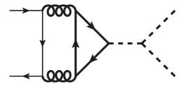
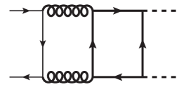
(a)	(b)

Figure 14: Sample Feynman diagrams for the process $q\bar{q}\to HH$.

In this appendix we discuss the virtual corrections to the process $q\bar{q}\to HH$. The coupling of the initial-state quark anti-quark pair to the Higgs bosons in the final state has to be mediated by top quarks. Thus at the lowest order it proceeds via two-loop diagrams such as those shown in Fig. 14. As a consequence such virtual corrections contribute for the first time at NNLO.

Diagrams involving a triple-Higgs boson coupling (cf. Fig. 14(a)) vanish for massless quarks $q$ since the (effective) coupling of the $q\bar{q}$ pair to one Higgs boson requires a helicity flip. However, diagrams such as the one in Fig. 14(b) can provide non-vanishing contributions. We have shown by an explicit calculation that such diagrams vanish in the $m_{t}\to\infty$ limit. However, non-vanishing contributions exist starting from $1/m_{t}^{2}$. In the following we describe their calculation and present the results.

In principle there are two methods to compute the total cross section. We can either compute the two-loop amplitude $q\bar{q}\to HH$ and integrate over the phase space, or we can consider five-loop forward-scattering $q\bar{q}\to q\bar{q}$ diagrams and take the imaginary part. We have used both approaches and have obtained identical results. Note that the real corrections to the $q\bar{q}$ channel discussed above are finite. Thus we expect the two-loop virtual corrections $q\bar{q}\to HH$ also to be finite.

We first describe the computation of the amplitude ${\cal M}(q\bar{q}\to HH)$. This is conveniently done using the projector

$$P_{q\bar{q}\to HH} = \frac{\delta^{ij}}{N_{c}}\frac{\not{q}_{1}\not{q}_{3}\not{q}_{2}}{2ut-2m_{H}^{4}}\,,$$ (92)

where $N_{c}=3$ and $q_{1}$ and $q_{2}$ are the incoming momenta of the quark and anti-quark, respectively, and $q_{3}$ is the incoming momentum of one of the Higgs bosons. $t=(q_{1}+q_{3})^{2}$ and $u=(q_{2}+q_{3})^{2}$ are Mandelstam variables and $i$ and $j$ are colour indices of the quark and anti-quark, respectively. Asymptotic expansion in the large-$m_{t}$ limit, which we apply with the help of exp [36, 37], leads to two-loop vacuum integrals and products of one-loop vacuum and one-loop massless form factor integrals. We perform the calculation with a general QCD gauge parameter and check that it drops out in the sum of all contributing diagrams. Next we square the amplitude obtain the differential cross section

$$\frac{{\rm d}\sigma_{q\bar{q}\to HH}}{{\rm d}{y}} = \frac{f^{\rm 2PS}(\epsilon)}{2\cdot N_{c}^{2}\cdot 2^{2}{\cdot 2s}}N_{c}(2ut-{2}m_{H}^{4})\left|{\cal M}^{\star}_{q\bar{q}\to HH}{\cal M}_{q\bar{q}\to HH}\right|\,,$$ (93)

where the denominators in the first factor are due to the two identical Higgs bosons in the final state, the colour and the spin averages, and the flux factor. The function $f^{\rm 2PS}(\epsilon)$ can be found in Eq. (19) and $y$ is defined in Eq. (20). The integrand is expanded in $\delta$, and we then perform the integration over $y$ for each expansion term separately. Our result for the total cross section up to terms of order $1/m_{t}^{6}$ ($\rho^{3}$) is given by

$$\sigma_{q\bar{q}\to HH} = \frac{a_{s}^{4}G_{F}^{2}m_{H}^{2}}{\pi}\Bigg{\{}\delta^{5/2}\rho^{2}\Bigg{(}\frac{22201}{2952450000}-\frac{1639\log 2}{73811250}+\frac{121\log^{2}2}{7381125}-\frac{1639\log\rho}{147622500}$$ (94)

$${}+\frac{121\log 2\log\rho}{7381125}+\frac{121\log^{2}\rho}{29524500}+\frac{121\pi^{2}}{29524500}\Bigg{)}+\delta^{5/2}\rho^{3}\Bigg{(}-\frac{588401}{124002900000}$$

$${}+\frac{5891\log 2}{6200145000}+\frac{22\log^{2}2}{2460375}+\frac{5891\log\rho}{12400290000}+\frac{22\log 2\log\rho}{2460375}+\frac{11\log^{2}\rho}{4920750}$$

$${}+\frac{11\pi^{2}}{4920750}\Bigg{)}+{\cal O}\left(\delta^{7/2}\right)+{\cal O}\left(\rho^{4}\right)\Bigg{\}}\,.$$

The ancillary files of this paper [62] contain the $\sigma_{q\bar{q}\to HH}$ expansion to $\rho^{4}$ and $\delta^{30}$.

An alternative approach to obtain the cross section $\sigma_{q\bar{q}\to HH}$ is based on the computation of the imaginary part of the forward scattering amplitude, which has been applied to the real corrections described in the main part of this paper. From the computational point of view this is much more demanding since we have to consider five-loop amplitudes which factorize into one- and two-loop vacuum contributions and one-loop form factor integrals. We have cross-checked Eq. (94) up to order $1/m_{t}^{6}$ ($\rho^{3}$) using this approach.

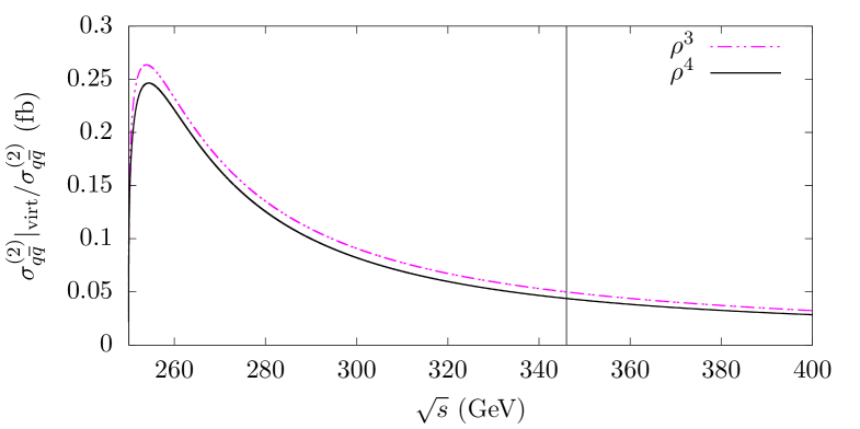
Figure 15: The ratio between the $q\bar{q}\to HH$ virtual corrections and the full $q\bar{q}$ cross section, as plotted in Fig. 13(c).

In Fig. 15 we show the size of $\sigma_{q\bar{q}\to HH}$ compared to $\sigma_{q\bar{q}}$. The virtual corrections form a significant part of the total cross section, particularly near the production threshold. Therefore they should be included for a proper NNLO description of the $q\bar{q}$ channel.

Appendix D Virtual NNLO corrections proportional to $n_{h}^{4}$

In this appendix we provide analytic results for the NNLO corrections which involve (in the forward-scattering kinematics) four closed top quark loops. Such $n_{h}^{4}$ terms are only present in the virtual corrections, see Fig. 11(h). The leading terms in the $\rho$ and $\delta$ expansion are given by

$$\sigma_{gg}^{(2),n_{h}^{4}} =\frac{a_{s}^{4}G_{F}^{2}m_{H}^{2}}{\pi}\Bigg{\{}\frac{\sqrt{\delta}}{20736}+\frac{\delta^{3/2}}{20736}+\rho\Bigg{(}-\frac{\sqrt{\delta}}{155520}-\frac{{13}\delta^{3/2}}{311040}\Bigg{)}+\mathcal{O}(\delta^{5/2})+\mathcal{O}(\rho^{2})\Bigg{\}}\,,$$ (95)

and all terms up to $\rho^{4}$ and $\delta^{30}$ can be found in the ancillary files of this paper [62].

Appendix E Explicit expressions for $\mathcal{Q}_{i}^{(3)}$ and $\mathcal{Q}_{i}^{(4)}$

In Tabs. 2 and 3 we provide explicit expressions for $Q_{i}^{(3)}$ and $Q_{i}^{(4)}$ introduced in Section 3.3, where the denominators as given by

$$D_{1} =-(-p_{5}+q_{1}+q_{2})^{2}\approx-s\,,$$

$$D_{2} =-(p_{5}-q_{1})^{2}\approx\frac{\kappa_{5}(1-\cos\theta_{5})s}{2}\,,$$

$$D_{3} =m_{H}^{2}-(p_{5}+p_{6}-q_{1}-q_{2})^{2}\approx-\frac{3s}{4}\,,$$

$$D_{4} =-(p_{4}+p_{5}+p_{6}-q_{1})^{2}\approx\frac{s}{4}\,,$$

$$D_{5} =-(p_{5}+p_{6})^{2}\approx-m_{gg}^{2}\,,$$

$$D_{6} =-(p_{6}-q_{1})^{2}\approx\frac{\kappa_{6}(1-\cos\theta_{6})s}{2}\,,$$

$$D_{7} =-(p_{5}+p_{6}-q_{1})^{2}\approx\frac{\kappa_{56}(1-\cos\theta_{56})s}{2}\,,$$

$$D_{8} =-(p_{5}-q_{2})^{2}\approx\frac{\kappa_{5}(1+\cos\theta_{5})s}{2}\,,$$

$$D_{9} =-(p_{6}-q_{2})^{2}\approx\frac{\kappa_{6}(1+\cos\theta_{6})s}{2}\,,$$

$$D_{10} =-(p_{5}+p_{6}-q_{2})^{2}\approx\frac{\kappa_{56}(1+\cos\theta_{56})s}{2}\,,$$

$$D_{11} =-(-p_{6}+q_{1}+q_{2})^{2}\approx-s\,.$$ (96)

After the symbol “$\approx$” the leading-order term in $\delta$ is given.

$i$	$Q^{(3)}_{i}$	$i$	$Q^{(3)}_{i}$	$i$	$Q^{(3)}_{i}$	$i$	$Q^{(3)}_{i}$	$i$	$Q^{(3)}_{i}$
1	$L_{1}$	2	$(D_{1}+m_{H}^{2})L_{1}$	3	$L_{2}$	4	$(D_{1}+m_{H}^{2})L_{2}$	5	$L_{3}$
6	$(D_{1}+m_{H}^{2})L_{3}$	7	$L_{4}$	8	$\frac{1}{D_{2}}L_{5}$	9	$\frac{(D_{1}+m_{H}^{2})}{D_{2}}L_{5}$	10	$L_{6}$
11	$(D_{1}+m_{H}^{2})L_{6}$	12	$\frac{1}{D_{1}+m_{H}^{2}}L_{1}$	13	$\frac{1}{D_{1}+m_{H}^{2}}L_{2}$	14	$\frac{1}{D_{1}+m_{H}^{2}}L_{3}$	15	$\frac{1}{D_{1}+m_{H}^{2}}L_{4}$
16	$\frac{1}{D_{2}(D_{1}+m_{H}^{2})}L_{5}$	17	$\frac{1}{D_{1}+m_{H}^{2}}L_{6}$

Table 2: $Q_{i}^{(3)}$ expressed in terms of the denominator factors from Eq. (96) and the integrals $L_{i}$ from Eqs. (36) and (3.3.1).

$i$	$Q^{(4)}_{i}$	$i$	$Q^{(4)}_{i}$	$i$	$Q^{(4)}_{i}$	$i$	$Q^{(4)}_{i}$	$i$	$Q^{(4)}_{i}$
1	$1$	2	$D_{3}$	3	$D_{4}$	4	$\frac{1}{D_{3}}$	5	$\frac{D_{4}}{D_{3}}$
6	$\frac{1}{D_{1}D_{7}}$	7	$\frac{D_{3}}{D_{1}D_{7}}$	8	$\frac{D_{8}}{D_{1}D_{7}}$	9	$\frac{1}{D_{1}D_{3}D_{7}}$	10	$\frac{D_{8}}{D_{1}D_{3}D_{7}}$
11	$\frac{1}{D_{1}D_{5}D_{7}D_{8}}$	12	$\frac{D_{3}}{D_{1}D_{5}D_{7}D_{8}}$	13	$\frac{1}{D_{1}D_{3}D_{5}D_{7}D_{8}}$	14	$\frac{1}{D_{10}D_{7}}$	15	$\frac{D_{3}}{D_{10}D_{7}}$
16	$\frac{1}{D_{10}D_{3}D_{7}}$	17	$\frac{1}{D_{10}D_{2}D_{7}D_{8}}$	18	$\frac{D_{3}}{D_{10}D_{2}D_{7}D_{8}}$	19	$\frac{1}{D_{10}D_{2}D_{3}D_{7}D_{8}}$	20	$\frac{1}{D_{2}D_{9}}$
21	$\frac{1}{D_{2}D_{3}D_{9}}$	22	$\frac{1}{D_{2}D_{6}D_{8}D_{9}}$	23	$\frac{D_{3}}{D_{2}D_{6}D_{8}D_{9}}$	24	$\frac{1}{D_{2}D_{3}D_{6}D_{8}D_{9}}$	25	$\frac{1}{D_{1}D_{11}}$
26	$\frac{D_{3}}{D_{1}D_{11}}$	27	$\frac{1}{D_{11}D_{8}}$	28	$\frac{1}{D_{1}D_{11}D_{3}}$	29	$\frac{1}{D_{11}D_{3}D_{8}}$	30	$\frac{1}{D_{1}D_{11}D_{8}D_{9}}$
31	$\frac{D_{3}}{D_{1}D_{11}D_{8}D_{9}}$	32	$\frac{1}{D_{1}D_{11}D_{3}D_{8}D_{9}}$	33	$\frac{1}{D_{1}D_{11}D_{6}D_{8}}$	34	$\frac{1}{D_{1}D_{11}D_{3}D_{6}D_{8}}$	35	$\frac{1}{D_{1}D_{6}}$
36	$\frac{1}{D_{1}D_{11}}$	37	$\frac{D_{3}}{D_{1}D_{11}}$	38	$\frac{1}{D_{1}D_{3}D_{6}}$	39	$\frac{1}{D_{1}D_{11}D_{3}}$	40	$\frac{1}{D_{1}D_{11}D_{2}D_{6}}$
41	$\frac{D_{3}}{D_{1}D_{11}D_{2}D_{6}}$	42	$\frac{1}{D_{1}D_{11}D_{2}D_{3}D_{6}}$	43	$\frac{1}{D_{1}D_{11}D_{6}D_{8}}$	44	$\frac{1}{D_{1}D_{11}D_{3}D_{6}D_{8}}$	45	$\frac{1}{D_{11}D_{8}}$
46	$\frac{1}{D_{10}D_{11}D_{8}}$	47	$\frac{D_{3}}{D_{10}D_{11}D_{8}}$	48	$\frac{1}{D_{11}D_{3}D_{8}}$	49	$\frac{1}{D_{10}D_{11}D_{3}D_{8}}$	50	$\frac{1}{D_{10}D_{11}D_{6}D_{8}}$
51	$\frac{1}{D_{10}D_{11}D_{3}D_{6}D_{8}}$	52	$\frac{1}{D_{10}D_{6}D_{7}D_{8}}$	53	$\frac{D_{3}}{D_{10}D_{6}D_{7}D_{8}}$	54	$\frac{1}{D_{10}D_{3}D_{6}D_{7}D_{8}}$	55	$\frac{1}{D_{5}D_{6}D_{8}}$
56	$\frac{D_{3}}{D_{5}D_{6}D_{8}}$	57	$\frac{1}{D_{3}D_{5}D_{6}D_{8}}$

Table 3: $Q_{i}^{(4)}$ expressed in terms of the denominator factors from Eq. (96).

References

- [1] G. Aad et al. [ATLAS], Phys. Lett. B 716 (2012), 1-29 [arXiv:1207.7214 [hep-ex]].
- [2] S. Chatrchyan et al. [CMS], Phys. Lett. B 716 (2012), 30-61 [arXiv:1207.7235 [hep-ex]].
- [3] P. A. Zyla et al. [Particle Data Group], PTEP 2020 (2020) no.8, 083C01.
- [4] G. Aad et al. [ATLAS], JHEP 07 (2020), 108 [erratum: JHEP 01 (2021), 145; erratum: JHEP 05 (2021), 207] [arXiv:2001.05178 [hep-ex]].
- [5] A. M. Sirunyan et al. [CMS], JHEP 03 (2021), 257 [arXiv:2011.12373 [hep-ex]].
- [6] E. W. N. Glover and J. J. van der Bij, Nucl. Phys. B 309 (1988) 282.
- [7] T. Plehn, M. Spira and P. M. Zerwas, Nucl. Phys. B 479 (1996) 46 Erratum: [Nucl. Phys. B 531 (1998) 655] [hep-ph/9603205].
- [8] S. Dawson, S. Dittmaier and M. Spira, Phys. Rev. D 58 (1998) 115012 [hep-ph/9805244].
- [9] J. Grigo, J. Hoff, K. Melnikov and M. Steinhauser, Nucl. Phys. B 875 (2013) 1 [arXiv:1305.7340 [hep-ph]].
- [10] G. Degrassi, P. P. Giardino and R. Gröber, Eur. Phys. J. C 76 (2016) no.7, 411 [arXiv:1603.00385 [hep-ph]].
- [11] J. Davies, G. Mishima, M. Steinhauser and D. Wellmann, JHEP 1803 (2018) 048 [arXiv:1801.09696 [hep-ph]].
- [12] J. Davies, G. Mishima, M. Steinhauser and D. Wellmann, JHEP 1901 (2019) 176 [arXiv:1811.05489 [hep-ph]].
- [13] R. Bonciani, G. Degrassi, P. P. Giardino and R. Gröber, Phys. Rev. Lett. 121 (2018) no.16, 162003 [arXiv:1806.11564 [hep-ph]].
- [14] R. Gröber, A. Maier and T. Rauh, JHEP 1803 (2018) 020 [arXiv:1709.07799 [hep-ph]].
- [15] F. Maltoni, E. Vryonidou and M. Zaro, JHEP 1411 (2014) 079 [arXiv:1408.6542 [hep-ph]].
- [16] S. Borowka, N. Greiner, G. Heinrich, S. P. Jones, M. Kerner, J. Schlenk, U. Schubert and T. Zirke, Phys. Rev. Lett. 117 (2016) no.1, 012001 Erratum: [Phys. Rev. Lett. 117 (2016) no.7, 079901] [arXiv:1604.06447 [hep-ph]].
- [17] S. Borowka, N. Greiner, G. Heinrich, S. P. Jones, M. Kerner, J. Schlenk and T. Zirke, JHEP 1610 (2016) 107 [arXiv:1608.04798 [hep-ph]].
- [18] J. Baglio, F. Campanario, S. Glaus, M. Mühlleitner, M. Spira and J. Streicher, Eur. Phys. J. C 79 (2019) no.6, 459 [arXiv:1811.05692 [hep-ph]].
- [19] J. Davies, G. Heinrich, S. P. Jones, M. Kerner, G. Mishima, M. Steinhauser and D. Wellmann, JHEP 11 (2019), 024 [arXiv:1907.06408 [hep-ph]].
- [20] J. Baglio, F. Campanario, S. Glaus, M. Mühlleitner, J. Ronca and M. Spira, Phys. Rev. D 103 (2021) no.5, 056002 [arXiv:2008.11626 [hep-ph]].
- [21] D. de Florian and J. Mazzitelli, Phys. Rev. Lett. 111 (2013) 201801 [arXiv:1309.6594 [hep-ph]].
- [22] D. de Florian and J. Mazzitelli, Phys. Lett. B 724 (2013) 306 [arXiv:1305.5206 [hep-ph]].
- [23] J. Grigo, K. Melnikov and M. Steinhauser, Nucl. Phys. B 888 (2014) 17 [arXiv:1408.2422 [hep-ph]].
- [24] J. Grigo, J. Hoff and M. Steinhauser, Nucl. Phys. B 900 (2015) 412 [arXiv:1508.00909 [hep-ph]].
- [25] J. Davies, F. Herren, G. Mishima and M. Steinhauser, JHEP 05 (2019), 157 [arXiv:1904.11998 [hep-ph]].
- [26] M. Grazzini, G. Heinrich, S. Jones, S. Kallweit, M. Kerner, J. M. Lindert and J. Mazzitelli, JHEP 1805 (2018) 059 [arXiv:1803.02463 [hep-ph]].
- [27] L. B. Chen, H. T. Li, H. S. Shao and J. Wang, Phys. Lett. B 803 (2020), 135292 [arXiv:1909.06808 [hep-ph]].
- [28] L. B. Chen, H. T. Li, H. S. Shao and J. Wang, JHEP 03 (2020), 072 [arXiv:1912.13001 [hep-ph]].
- [29] C. Anastasiou, C. Duhr, F. Dulat, E. Furlan, T. Gehrmann, F. Herzog, A. Lazopoulos and B. Mistlberger, JHEP 05 (2016), 058 [arXiv:1602.00695 [hep-ph]].
- [30] B. Mistlberger, JHEP 05 (2018), 028 [arXiv:1802.00833 [hep-ph]].
- [31] M. Spira, JHEP 1610 (2016) 026 [arXiv:1607.05548 [hep-ph]].
- [32] M. Gerlach, F. Herren and M. Steinhauser, JHEP 1811 (2018) 141 [arXiv:1809.06787 [hep-ph]].
- [33] P. Banerjee, S. Borowka, P. K. Dhani, T. Gehrmann and V. Ravindran, JHEP 1811 (2018) 130 [arXiv:1809.05388 [hep-ph]].
- [34] P. Nogueira, J. Comput. Phys. 105 (1993) 279.
- [35] A. Pak, unpublished.
- [36] R. Harlander, T. Seidensticker and M. Steinhauser, Phys. Lett. B 426 (1998) 125 [hep-ph/9712228].
- [37] T. Seidensticker, hep-ph/9905298.
- [38] B. Ruijl, T. Ueda and J. Vermaseren, arXiv:1707.06453 [hep-ph].
- [39] M. Steinhauser, Comput. Phys. Commun. 134 (2001) 335 [arXiv:hep-ph/0009029].
- [40] J. Davies, F. Herren, G. Mishima and M. Steinhauser, PoS RADCOR2019 (2019), 022 [arXiv:1912.01646 [hep-ph]].
- [41] F. Herren, “Precision Calculations for Higgs Boson Physics at the LHC - Four-Loop Corrections to Gluon-Fusion Processes and Higgs Boson Pair-Production at NNLO,” PhD thesis, 2020, KIT.
- [42] A. Pak, J. Phys. Conf. Ser. 368 (2012), 012049 [arXiv:1111.0868 [hep-ph]].
- [43] R. N. Lee, arXiv:1212.2685 [hep-ph].
- [44] R. N. Lee, J. Phys. Conf. Ser. 523 (2014) 012059 [arXiv:1310.1145 [hep-ph]].
- [45] G. Altarelli and G. Parisi, Nucl. Phys. B 126 (1977), 298-318
- [46] G. Curci, W. Furmanski and R. Petronzio, Nucl. Phys. B 175 (1980), 27-92
- [47] S. Moch, J. A. M. Vermaseren and A. Vogt, Nucl. Phys. B 688 (2004), 101-134 [arXiv:hep-ph/0403192 [hep-ph]].
- [48] A. Vogt, S. Moch and J. A. M. Vermaseren, Nucl. Phys. B 691 (2004), 129-181 [arXiv:hep-ph/0404111 [hep-ph]].
- [49] C. Anastasiou and K. Melnikov, Nucl. Phys. B 646 (2002), 220-256 [arXiv:hep-ph/0207004 [hep-ph]].
- [50] M. Höschele, J. Hoff, A. Pak, M. Steinhauser and T. Ueda, Comput. Phys. Commun. 185 (2014), 528-539 [arXiv:1307.6925 [hep-ph]].
- [51] J. Davies and M. Steinhauser, JHEP 10 (2019), 166 [arXiv:1909.01361 [hep-ph]].
- [52] A. V. Kotikov, Phys. Lett. B 254 (1991), 158-164
- [53] T. Gehrmann and E. Remiddi, Nucl. Phys. B 580 (2000), 485-518 [arXiv:hep-ph/9912329 [hep-ph]].
- [54] J. M. Henn, Phys. Rev. Lett. 110 (2013), 251601 [arXiv:1304.1806 [hep-th]].
- [55] A. B. Goncharov, Math. Res. Lett. 5 (1998), 497-516 [arXiv:1105.2076 [math.AG]].
- [56] R. N. Lee, [arXiv:2012.00279 [hep-ph]].
- [57] R. N. Lee, JHEP 04 (2015), 108 [arXiv:1411.0911 [hep-ph]].
- [58] M. Beneke and V. A. Smirnov, Nucl. Phys. B 522 (1998), 321-344 [arXiv:hep-ph/9711391 [hep-ph]].
- [59] A. Pak and A. Smirnov, Eur. Phys. J. C 71 (2011), 1626 [arXiv:1011.4863 [hep-ph]].
- [60] B. Jantzen, A. V. Smirnov and V. A. Smirnov, Eur. Phys. J. C 72 (2012), 2139 [arXiv:1206.0546 [hep-ph]].
- [61] V. A. Smirnov, “Feynman integral calculus,” Springer (2006)
-
[62]
https://www.ttp.kit.edu/preprints/2021/ttp21-034/. - [63] K. Melnikov, L. Tancredi and C. Wever, JHEP 11 (2016), 104 [arXiv:1610.03747 [hep-ph]].
- [64] G. Mishima, JHEP 02 (2019), 080 [arXiv:1812.04373 [hep-ph]].
- [65] J. Davies, R. Gröber, A. Maier, T. Rauh and M. Steinhauser, Phys. Rev. D 100 (2019) no.3, 034017 [erratum: Phys. Rev. D 102 (2020) no.5, 059901] [arXiv:1906.00982 [hep-ph]].
- [66] J. Davies, R. Gröber, A. Maier, T. Rauh and M. Steinhauser, PoS RADCOR2019 (2019), 079 [arXiv:1912.04097 [hep-ph]].
- [67] M. Höschele, J. Hoff, A. Pak, M. Steinhauser and T. Ueda, Comput. Phys. Commun. 185 (2014), 528-539 [arXiv:1307.6925 [hep-ph]].