All-order renormalization of electric charge
in the Standard Model and beyond
Stefan Dittmaier
Albert-Ludwigs-Universität Freiburg, Physikalisches Institut, D-79104 Freiburg, Germany
* stefan.dittmaier@physik.uni-freiburg.de
![[Uncaptioned image]](/html/2109.03528/assets/RADCOR_LoopFest_2021_web.jpg) 15th International Symposium on Radiative Corrections:
15th International Symposium on Radiative Corrections:
Applications of Quantum Field Theory to Phenomenology,
FSU, Tallahasse, FL, USA, 17-21 May 2021
10.21468/SciPostPhysProc.?
Abstract
Electric charge, as defined in the Thomson limit of the electron–photon interaction vertex, is renormalized to all orders both in the Standard Model and in any spontaneously broken gauge theory with gauge group U(1) with a group factor U(1) that mixes with electromagnetic gauge symmetry. In the framework of the background-field method the charge renormalization constant is directly obtained from the photon wave-function renormalization constant, similar to the situation in QED, which proves charge universality as a byproduct. Exploiting charge universality in arbitrary gauge by formulating the charge renormalization condition for a “fake fermion” that couples only via an infinitesimal electric charge, can be expressed in terms of renormalization constants that are obtained solely from gauge-boson self-energies.
1 Introduction
The definition of electric unit charge is carried over from classical electrodynamics to quantum electrodynamics (QED) and to more comprehensive quantum field theories such as the Standard Model (SM) upon imposing the Thomson renormalization condition which demands that the electron–photon interaction vertex for physical (on-shell) electrons does not receive any radiative corrections in the limit of low-energy photons. The charge renormalization constant , which relates the bare charge to the renormalized unit charge , can, thus, be determined from the ee vertex correction in this limit by direct calculation of this correction in a given perturbative order. Exploiting electromagnetic gauge invariance in the form of the famous Ward identity for the ee vertex, in QED it is possible to calculate from the wave-function renormalization constant of the photon, i.e. merely from a self-energy. This is not only a welcome technical simplification, but also an important field-theoretical result that is helpful in proving structural theorems such as charge universality or Thirring’s theorem for low-energy Compton scattering [1, 2]. Charge universality is the non-trivial statement that the renormalized unit charge does not depend on the fermion species (actually not even on the type of charged particle) that is used in the formulation of the Thomson renormalization condition on the vertex.
In the SM and most of its extensions, the derivation of from self-energies is very complicated (and not known beyond the one-loop level) if the derivation is directly based on gauge invariance, which manifests itself via Slavnov–Taylor identities for Green functions and Lee identities for (one-particle irreducible, 1PI) vertex functions. This is due to the fact that the unbroken electromagnetic U(1)em gauge symmetry is not a mere factor of the gauge group, but mixes with a non-abelian subgroup in a non-trivial way. Other U(1) group factors, such as the weak hypercharge group in the SM, which mix with electromagnetic gauge symmetry cannot fully play the role of U(1)em of QED, because they are spontaneously broken. Owing to this difficulty, in the early pioneering proposals for electroweak one-loop renormalization [3, 4, 5, 6, 7, 8, 9, 10] the derivation of was either based on explicit calculations of the vertex correction or on Ward identities that were verified by explicit calculations. A derivation fully based on Lee identities at one loop without any explicit loop calculation has only been given quite recently [11];111An alternative proof based on Slavnov–Taylor identities is sketched in the slides of the corresponding talk given at the conference. owing to its complexity a generalization of this approach beyond the one-loop level seems rather complicated, if not infeasible.
The first all-order result for in the SM, again expressed in terms of the photon wave-function renormalization constant, was given in the framework of the background-field method (BFM) in Ref. [12]. This result, in particular, proves charge universality in the SM to all orders. In Ref. [13] it was shown by explicit calculation that the BFM result for indeed is in line with the Thomson condition for the electron–photon vertex at the two-loop level in arbitrary gauge. Similarly, in Refs. [14, 15, 16] it was shown by explicit two-loop calculation in conventional ’t Hooft–Feynman gauge that the sum of all genuine vertex corrections and fermionic wave-function corrections to the vertex vanishes in the Thomson limit; this is exactly the part in the calculation of that is ruled by gauge invariance but not yet proven on the basis of Slavnov–Taylor or Lee identities to all orders. In fact a general result on expressed in terms of other renormalization constants that are related to gauge-boson self-energies, was suggested in Ref. [17]—although correct, this result was actually more conjectured than derived.222Detailed comments on the arguments given in Ref. [17] can be found in the appendix of Ref. [18]. This form of was subsequently used in the few existing explicit electroweak two-loop calculations, such as for the muon decay [19, 20] or Z-boson decay widths [21].
After briefly sketching the BFM derivation of within the SM to all orders, in the following we review the all-order derivation [18] of within arbitrary gauge, exploiting charge universality by imposing the Thomson renormalization condition on the electromagnetic interaction vertex of a “fake fermion” with infinitesimal electric charge but no other charges or couplings, so that fully decouples from all other particles for . We first describe the derivation within the SM, where the result confirms the earlier “conjecture” of Ref. [17], and then generalize it to a more general gauge group U(1), where is any compact Lie group and U(1) has an admixture of electromagnetic gauge symmetry. This article is just a brief summary of Ref. [18], where a much more complete treatment of the subject can be found.
2 Charge renormalization and charge universality in the background-field method
Denoting the relative charge and mass of the fermion by and , respectively, the Thomson renormalization condition reads
| (1) |
where is the background photon field and the renormalized vertex function in the BFM. Here and are Dirac spinors of the fermion with momentum fulfilling with the renormalized on-shell mass . In the notation and conventions for all field-theoretical quantities we follow Ref. [11] throughout.
The needed low-energy limit of the for on-shell fermions can be obtained from its BFM Ward identity, which follows from the background-field gauge invariance of the BFM effective action (see Refs. [12, 11] and references therein). This Ward identity for the unrenormalized vertex function reads [12]333We ignore fermion generation mixing here; for its restoration see Ref. [18].
| (2) |
where is the unrenormalized two-point vertex function of the fermions. To exploit this identity in condition (1), we have to replace unrenormalized by renormalized quantities. Indicating bare quantities consistently by subscripts 0, the relevant parts of this renormalization transformation reads
| (3) |
where refers to the right- and left-handed parts of the fermion field and is the background Z-boson field. The resulting relation between renormalized and unrenormalized vertex functions reads
| (4) | ||||
| (5) |
The introduced field-renormalization constants for the fermions and for the photon–Z-boson system are fixed by on-shell (OS) renormalization conditions, which require canonical normalization of the residues of particle propagators and eliminates mixing between different fields for on-shell momenta. Background-field gauge invariance automatically implies (see, e.g., Refs. [12, 11] for more details). Using additionally , turns the Ward identity (2) into an analogous identity for renormalized quantities,
| (6) |
which is valid for arbitrary momenta , , obeying . Taking for fixed , the terms linear in obey the relation
| (7) |
Sandwiching this relation between Dirac spinors, its l.h.s. becomes identical to the one of (7), and its r.h.s. can be simplified with the OS renormalization condition for the fermion field, which can be written as
| (8) |
Thus, combining the charge renormalization condition (1) with (7) and (8) leads to the simple equation [12]
| (9) |
in the BFM, which is formally identical to the well-known relation in QED. Note also that Eq. (9) shows that , i.e. that the product of electromagnetic coupling and background photon field is not renormalized, again in analogy to a QED relation.
3 Charge renormalization in arbitrary -gauge
We now extend the SM by adding a fermion field with vanishing weak isospin, , and weak hypercharge . Taking the limit of vanishing electric charge, , the fermion decouples from all other particles, and we recover the original theory—therefore the terminology “fake fermion”. The Lagrangian of the SM is, thus, modified by adding
| (10) |
with denoting the arbitrary mass of the fermion . We note that the mass term for is gauge invariant, that is stable, and that no anomalies are introduced owing to the non-chirality of . As in the SM, is the U(1)Y gauge coupling, the U(1)Y gauge field, and and the sine and cosine of the weak mixing angle . Employing charge universality, we can take the Thomson limit of the vertex to define the renormalized electric unit charge ,
| (11) |
The relation between and its bare counterpart follows from the field renormalization transformation and the analog of (3) for the photon–Z-boson system and reads
| (12) |
The bare vertex functions () receive lowest-order contributions and bare vertex corrections , which consist of 1PI loop diagrams and tadpole corrections,
| (13) |
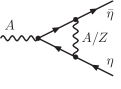
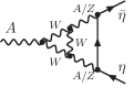
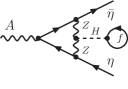
The important observation is now that all diagrammatic contributions to and involve at least two couplings of photons or Z bosons to the line that passes through the whole diagram. Some sample diagrams are shown in Fig. 1.
(a)
 (b)
(b)
 (c)
(c)
(d)
 (e)
(e)
 (f)
(f)
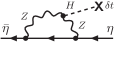
For 1PI diagrams it is obvious that at least two couplings to the line exist, for diagrams with tadpole loops or tadpole counterterms the same holds true, because the Higgs field does not couple to . Since both the photon and the Z boson couple to proportional to , this means that and . Inserting, thus, from (12) into condition (11) and keeping only terms linear in for , we get
| (14) |
This relation implies
| (15) |
which is the desired relation between and . Introducing the renormalization constant according to
| (16) |
we can determine from (15),
| (17) |
This is fully equivalent to the result quoted and used in Refs. [17, 19, 20]. Since vanishes at tree level, the renormalization constant is only required to -loop order in the -loop calculation of .
4 Generalization to non-standard gauge groups
The concept of charge universality and charge renormalization outlined above for the SM can be generalized easily to gauge groups of the type U(1), where is any compact Lie group of rank and the U(1) group factor plays the analogous role of weak hypercharge in the SM. More precisely, we mean by this that the U(1)em subgroup of electromagnetic gauge symmetry mixes transformations of U(1) and , so that the photon field is a non-trivial linear combination of the U(1) gauge field and the gauge fields () of corresponding to the diagonal group generators in the Lie algebra of . For the mechanism of electroweak symmetry breaking we only assume that electromagnetic gauge invariance is unbroken.
The original gauge fields and can be transformed into fields that correspond to mass eigenstates,
| (18) |
where () describe neutral massive gauge bosons similar to the Z boson of the SM. The matrix is a generalization of the SM rotation matrix parametrized by the weak mixing angle, but is not necessarily orthogonal or unitary. The OS renormalization of the gauge fields proceeds exactly as in the SM, with an obvious generalization of the matrix of renormalization constants of (3) to a matrix. The constants can be computed from the gauge-boson self-energies order by order.
The BFM derivation of the charge renormalization constant generalizes to the more general gauge group without any problems. Background-field gauge invariance implies for all , i.e. there is no mixing of on-shell photons with any of the Zk bosons. The Ward identities (2) and (6), thus, carry over without modification. As a result, the charge renormalization constant is given by as in (9), proving charge universality as in the SM.
To exploit charge universality in the determination of in arbitrary -gauge, we again introduce a fake fermion with the same properties as above, i.e. only carries infinitesimal U(1) charge , but no non-trivial quantum number of , so that the unit charge is given by . If the model contains singlet scalars , the scalars may couple to via Yukawa couplings. The corresponding couplings are free parameters of the model and can be taken to be infinitesimally small in analogy to , so that decoupling of is guaranteed. The Lagrangian reads
| (19) |
Following the same reasoning as for the SM above, the renormalized vertex function is given by
| (20) |
with the unrenormalized vertex functions
| (21) |
Again the vertex corrections and as well as the field renormalization constant receive only corrections that are suppressed at least by quadratic factors in the new couplings, such as or . Typical diagrams contributing to those corrections at the order (or higher in ) can be obtained from the graphs shown in Fig. 1 upon interpreting the field as any of the and taking the Higgs field as a any Higgs field of the model. Equation (3) then generalizes to the considered model in an obvious way, and we obtain the final result for the charge renormalization constant:
| (22) |
where and are renormalization constants for the matrix elements of , i.e. . Recalling that the constants vanish at tree level, we see that the constants and are only required to -loop order in the -loop calculation of .
The case of the SM is trivially recovered from the results of this section upon identifying SU(2)w, , , , and .
5 Conclusion
Employing the property of charge universality, the determination of the charge renormalization constant in arbitrary gauge can be greatly simplified upon applying the Thomson renormalization condition to a “fake fermion” that has infinitesimal electric charge but no other charges or couplings. Both in the SM and in the wider class of gauge theories with gauge group U(1), where the U(1) subgroup contains some component of electromagnetic gauge transformations, can be deduced from gauge-boson wave-function and parameter renormalization constants which can be calculated from gauge-boson self-energies only. Using Slavnov–Taylor or Lee identities to derive this result is already very cumbersome at the one-loop level, and a consistent generalization beyond one loop is not known, if not infeasible.
The assumed property of charge universality can for instance proven in the framework of the background-field method from which it is known that can be directly obtained from the photon wave-function renormalization constant.
For even more general gauge groups without a U(1) factor mixing with electromagnetic gauge symmetry, the strategy with the decoupling “fake fermion” seems not to be applicable. In this case the consistent use of the background-field method, however, still bears the possibility to calculate the charge renormalization constant in terms of gauge-boson wave-function renormalization constants in contrast to conventional -like gauges.
References
- [1] W. E. Thirring, Radiative corrections in the nonrelativistic limit, Phil. Mag. Ser. 7 41, 1193 (1950).
- [2] S. Dittmaier, Thirring’s low-energy theorem and its generalizations in the electroweak standard model, Phys. Lett. B 409, 509 (1997), 10.1016/S0370-2693(97)00888-5, hep-ph/9704368.
- [3] D. A. Ross and J. C. Taylor, Renormalization of a unified theory of weak and electromagnetic interactions, Nucl. Phys. B 51, 125 (1973), 10.1016/0550-3213(73)90505-1, [Erratum: Nucl.Phys.B 58, 643–643 (1973)].
- [4] A. Sirlin, Radiative Corrections in the SU(2)-L x U(1) Theory: A Simple Renormalization Framework, Phys. Rev. D 22, 971 (1980), 10.1103/PhysRevD.22.971.
- [5] D. Y. Bardin, P. K. Khristova and O. M. Fedorenko, On the Lowest Order Electroweak Corrections to Spin 1/2 Fermion Scattering. 1. The One Loop Diagrammar, Nucl. Phys. B 175, 435 (1980), 10.1016/0550-3213(80)90021-8.
- [6] J. Fleischer and F. Jegerlehner, Radiative Corrections to Higgs Decays in the Extended Weinberg-Salam Model, Phys. Rev. D 23, 2001 (1981), 10.1103/PhysRevD.23.2001.
- [7] K. I. Aoki, Z. Hioki, M. Konuma, R. Kawabe and T. Muta, Electroweak Theory. Framework of On-Shell Renormalization and Study of Higher Order Effects, Prog. Theor. Phys. Suppl. 73, 1 (1982), 10.1143/PTPS.73.1.
- [8] M. Böhm, H. Spiesberger and W. Hollik, On the One Loop Renormalization of the Electroweak Standard Model and Its Application to Leptonic Processes, Fortsch. Phys. 34, 687 (1986), 10.1002/prop.19860341102.
- [9] W. F. L. Hollik, Radiative Corrections in the Standard Model and their Role for Precision Tests of the Electroweak Theory, Fortsch. Phys. 38, 165 (1990), 10.1002/prop.2190380302.
- [10] A. Denner, Techniques for calculation of electroweak radiative corrections at the one loop level and results for W physics at LEP-200, Fortsch. Phys. 41, 307 (1993), 10.1002/prop.2190410402, 0709.1075.
- [11] A. Denner and S. Dittmaier, Electroweak Radiative Corrections for Collider Physics, Phys. Rept. 864, 1 (2020), 10.1016/j.physrep.2020.04.001, 1912.06823.
- [12] A. Denner, G. Weiglein and S. Dittmaier, Application of the background field method to the electroweak standard model, Nucl. Phys. B 440, 95 (1995), 10.1016/0550-3213(95)00037-S, hep-ph/9410338.
- [13] G. Degrassi and A. Vicini, Two loop renormalization of the electric charge in the standard model, Phys. Rev. D 69, 073007 (2004), 10.1103/PhysRevD.69.073007, hep-ph/0307122.
- [14] S. Actis, A. Ferroglia, M. Passera and G. Passarino, Two-Loop Renormalization in the Standard Model. Part I: Prolegomena, Nucl. Phys. B 777, 1 (2007), 10.1016/j.nuclphysb.2007.04.021, hep-ph/0612122.
- [15] S. Actis and G. Passarino, Two-Loop Renormalization in the Standard Model Part II: Renormalization Procedures and Computational Techniques, Nucl. Phys. B 777, 35 (2007), 10.1016/j.nuclphysb.2007.03.043, hep-ph/0612123.
- [16] S. Actis and G. Passarino, Two-Loop Renormalization in the Standard Model Part III: Renormalization Equations and their Solutions, Nucl. Phys. B 777, 100 (2007), 10.1016/j.nuclphysb.2007.04.027, hep-ph/0612124.
- [17] S. Bauberger, Two-loop contributions to muon decay, Phd thesis, Würzburg U. (1997).
- [18] S. Dittmaier, Electric charge renormalization to all orders, Phys. Rev. D 103(5), 053006 (2021), 10.1103/PhysRevD.103.053006, 2101.05154.
- [19] A. Freitas, W. Hollik, W. Walter and G. Weiglein, Electroweak two loop corrections to the mass correlation in the standard model, Nucl. Phys. B 632, 189 (2002), 10.1016/S0550-3213(02)00243-2, [Erratum: Nucl.Phys.B 666, 305–307 (2003)], hep-ph/0202131.
- [20] M. Awramik, M. Czakon, A. Onishchenko and O. Veretin, Bosonic corrections to Delta r at the two loop level, Phys. Rev. D 68, 053004 (2003), 10.1103/PhysRevD.68.053004, hep-ph/0209084.
- [21] I. Dubovyk, A. Freitas, J. Gluza, T. Riemann and J. Usovitsch, Complete electroweak two-loop corrections to Z boson production and decay, Phys. Lett. B 783, 86 (2018), 10.1016/j.physletb.2018.06.037, 1804.10236.