Bosonic Corrections to $\Delta r$ at the Two Loop Level

Abstract

The details of the recent calculation of the two-loop bosonic corrections to the muon lifetime in the Standard Model are presented. The matching on the Fermi theory is discussed. Renormalisation in the on-shell and in the $\overline{\text{MS}}$ scheme is studied and transition between the schemes is shown to lead to identical results. High precision numerical methods are compared with mass difference and large mass expansions.

I Introduction

The muon decay lifetime ($\tau_{\mu}$) has been used for long as an input parameter for high precision predictions of the Standard Model (SM). It allows for an indirect determination of the mass of the $W$ boson ($M_{W}$), which suffers currently from a large experimental error of 39 MeV Hagiwara:pw , one order of magnitude worse than that of the $Z$ boson mass ($M_{Z}$). A reduction of this error by LHC to 15 MeV lhctdr and by a future linear collider to 6 MeV tesla-tdr would provide a stringent test of the SM by confronting the theoretical prediction with the experimental value.

The extraction of $M_{W}$ with an accuracy matching that of next experiments, i.e. at the level of a few MeV necessitates radiative corrections beyond one loop order. Large two-loop contributions from fermionic loops have been calculated in Freitas:2000gg . The current prediction is affected by two types of uncertainties. First, apart from the still unknown Higgs boson mass, two input parameters introduce large errors. The current knowledge of the top quark mass results in an error of about 30 MeV Freitas:2002ja , which should be reduced by LHC to 10 MeV and by a linear collider even down to 1.2 MeV. The inaccuracy of the knowledge of the running of the fine structure constant up to the $M_{Z}$ scale, $\Delta\alpha(M_{Z})$, introduces a further $6.5$ MeV error. Second, several higher order corrections are unknown. In fact the last unknown correction at the ${\cal O}(\alpha^{2})$ order has been calculated only recently in my and oni . This contribution comes from diagrams with no closed fermion loops.

It is the purpose of the present work to give a detailed description of the methods used in the calculations presented in my and oni . Since one of the groups used high precision numeric methods and the other deep expansions both in mass differences and in large masses, a comparison can be given.

In the next section we discuss the question of matching of the Fermi theory onto the Standard Model at low energy scales. Then we move to the discussion of renormalisation in the on-shell scheme and continue with the $\overline{\text{MS}}$ scheme. A section on the transition between the schemes contains comparisons of the methods and the final results. The description of computational methods and conclusions close the main part of the work. In the appendices, a derivation of the electric charge counterterm through the $U(1)$ Ward identity can found, followed by the explicit analytic results of the expansions of the on-shell and the $\overline{\text{MS}}$ quantities.

II Matching

The muon lifetime $\tau_{\mu}$ can be computed from the effective Fermi theory given by the lagrangian

$${\cal L}^{\rm eff}={\cal L}_{\rm QED}+\frac{G_{F}}{\sqrt{2}}\,O_{F}+\mbox{higher dimension operators}\,,$$ (1)

where $O_{F}$ is the 4-fermion Fermi operator of dimension six

$$O_{F}=\bigl{[}\bar{\nu}_{\mu}\gamma^{\alpha}(1-\gamma_{5})\mu\bigr{]}\,\bigl{[}\bar{e}\gamma_{\alpha}(1-\gamma_{5})\nu_{e}\bigr{]},$$ (2)

and $G_{F}$ is the Fermi constant. Note that Eq. 1 is a definition of $G_{F}$. This lagrangian can be used to describe low energy processes (such that energies are $\ll M_{W}$) mediated by the weak charged current. Since the theory Eq. 1 is nonrenormalisable, an ultraviolet cut-off $\Lambda$ should be introduced.

In particular for the muon decay process we have

$$\frac{1}{\tau_{\mu}}=\frac{G_{F}^{2}m_{\mu}^{5}}{192\pi^{3}}\left(1-8\frac{m_{e}^{2}}{m_{\mu}^{2}}\right)(1+\Delta q)\,,$$ (3)

with $m_{e}$ and $m_{\mu}$ being the masses of the electron and the muon respectively. The quantity $\Delta q$ describes all QED corrections in the Fermi theory and has been calculated at the one-loop Berman:1958ti and at the two-loop vanRitbergen:1998yd order.

By its nature $G_{F}$ is the Wilson coefficient function of the operator $O_{F}$ and can be evaluated from the SM. Traditionally the matching relation between $G_{F}$ and the parameters of the SM is parametrised as follows

$$\frac{G_{F}}{\sqrt{2}}=\frac{e^{2}}{8(1-M_{W}^{2}/M_{Z}^{2})M_{W}^{2}}(1+\Delta r).$$ (4)

The quantity $\Delta r=\Delta r^{(1)}+\Delta r^{(2)}+\dots$ absorbs the effects of all loop diagrams.

It is the purpose of the following subsection to establish the framework for the calculation of $\Delta r$.

II.1 Factorisation theorem

In principle, the muon decay amplitude can be evaluated directly in the SM, but this is not feasible in practice. There are many scales involved which vary from less than 1 MeV to 100 GeV, i.e. by more than 5 orders of magnitude! On the other hand the number of Feynman diagrams grows very fast with the number of loops. A way out to keep the problem manageable is to switch on the machinery of effective lagrangians (see Eq. 1). This allows one to simplify the calculation enormously and to separate consistently the low energy (“soft”) dynamics from high energy (“hard”) static characteristics.

Suppose that we can compute the muon decay amplitude $A^{\text{SM}}$ in the SM. Then the Fermi constant $G_{F}$ defined through Eq. 1 can be predicted from $A^{\text{SM}}$. Indeed we should require that both evaluations in the SM and the Fermi theory give the same result. At the tree level the corresponding matching equation reads

$$A^{\text{SM}}=\frac{G_{F}}{\sqrt{2}}\,\langle\mu|O_{F}|e\nu_{\mu}\bar{\nu_{e}}\rangle+{\cal O}\left(\frac{m_{\mu}^{4}}{M_{W}^{4}}\right)\,.$$ (5)

This equation just states that the amplitude of the process $\mu\to e\nu\bar{\nu}$ is the same both in the full SM and in the effective Fermi theory up to operators of higher dimension.

When loop effects are taken into account, matrix elements in both sides of Eq. 5 get quantum corrections. Since $A^{\text{SM}}$ and $\langle\mu|O_{F}|e\nu_{\mu}\bar{\nu_{e}}\rangle$ are amputated matrix elements one has to renormalise also the external wave functions. Therefore the final form of the matching equation reads

$$\sqrt{Z_{2,e}^{\text{SM}}Z_{2,\mu}^{\text{SM}}Z_{2,\nu_{e}}^{\text{SM}}Z_{2,\nu_{\mu}}^{\text{SM}}}\,\,A^{\text{SM}}=\sqrt{Z_{2,e}^{\text{eff}}Z_{2,\mu}^{\text{eff}}Z_{2,\nu_{e}}^{\text{eff}}Z_{2,\nu_{\mu}}^{\text{eff}}}\,Z_{O_{F}}^{-1}\,\,\frac{G_{F}}{\sqrt{2}}\,\langle\mu|O_{F}|e\nu_{\mu}\bar{\nu_{e}}\rangle+{\cal O}\left(\frac{m_{\mu}^{4}}{M_{W}^{4}}\right)\,,$$ (6)

where $Z_{2,f}^{\text{SM}}$ and $Z_{2,f}^{\text{eff}}$ are wave function renormalisation constants of the fermions evaluated in the SM and in the effective theory respectively and $Z_{O_{F}}$ is the renormalisation constant of the Fermi operator in the effective theory.

There are two ways to compute $G_{F}$ from the SM:

1. standard matching calculation, or

2. automatic matching via factorisation theorem.

The former approach works always by simply computing all ingredients (apart from $G_{F}$) in the matching equation Eq. 6. This requires however much extra efforts to evaluate the “soft” pieces (or, at least, to separate them) in the amplitudes and the $Z$’s. Historically for this purpose the Pauli–Villars regularisation was used in Sirlin1 and then extended to two-loop order in Sirlin2 . The same approach has been applied also in Freitas:2002ja .

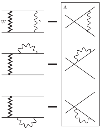
Figure 1: one-loop factorisation with Pauli-Villars regularisation.

How it works at the 1-loop level is demonstrated in Fig. 1. There are only three infrared divergent diagrams with photon. From each diagram its counterpart in the Fermi theory should be subtracted. The left diagram in each line of Fig. 1 corresponds to the result in the full model and therefore contains both the “soft” and the “hard” part. The right one contains only the “soft” part, which means that the difference is the requested “hard” correction. In addition, for the diagrams in the frame the Pauli-Villars regularisation is introduced to regularise the ultraviolet divergences. At the two-loop level we have a very similar situation. The difference is that instead of “hard” and “soft‘’ terms there are now “hard-hard”, “hard-soft”, “soft-hard” and “soft-soft” contributions. From these only the “hard-hard” piece contributes to $G_{F}$.

Accidentally, it happens that the sum of the three “soft” diagrams inside the frame in Fig. 1 is an ultraviolet finite quantity (let us call it $\Sigma_{\text{soft}}$). It is easy to prove that this holds true also to all orders. This is a consequence of the Ward–Takahashi identity for $QED$. This fact, however, is a pure coincidence rather than something fundamental. If such a cancelation had not occurred, renormalisation of the operator $O_{F}$ would be required as it is taken into account in Eq. 6.

The scheme given in Fig. 1 is consistent but the disadvantage of it is that there arises the problem of bookkeeping of “soft” and “hard” parts and already at the two-loop level the problem becomes very complicated. Indeed, at the two-loop level one has to subtract from each diagram the “hard-soft”, “soft-hard” and “soft-soft” pieces.

Therefore it would be very helpful to find some other way to obtain the “hard” part. Thus we come to the second way to compute $G_{F}$—automatic matching. This procedure is the most straightforward and the most economical (minimal in costs) way to compute. It is based on the factorisation theorem, proven e.g. in Gorishnii . It allows one to extract the “hard” part directly without any reference to “soft” pieces. As a well known example of such a procedure we can mention the evaluation of Wilson coefficient functions in deep inelastic scattering processes.

Returning to the sum of the three “soft” graphs in Fig. 1 ($\Sigma_{\text{soft}}$) we notice that in $G_{F}$ all “soft” modes are eliminated. This means, that all subgraphs in Fig. 1 should be computed at vanishing masses of the leptons. In this case the Ward–Takahashi identity not only makes $\Sigma_{\text{soft}}$ ultraviolet finite but also nullifies it. Thus all “soft” parts add up to zero. This is also true to all orders of perturbation theory. In other words, one can from the very beginning nullify all external momenta and masses and evaluate the obtained bubble diagrams. Of course new infrared divergences are generated. They cancel however in the expression for $G_{F}$. To regularise these infrared divergences we use the dimensional regularisation.

To prove rigorously that infrared singularities indeed drop out from the result one can turn to the framework for construction of effective low energy lagrangians given in Gorishnii . At the level of individual Feynman diagrams one can separate “soft” and “hard” scales with the help of the asymptotic expansion procedure asymptotic . Let $F$ denote a Feynman diagram. Then

$$F\sim\sum\limits_{H\subseteq F}S\cdot T(H)\,,$$ (7)

where the sum runs over all “hard” subgraphs $H$ of the diagram $F$; $S$ is a “soft” subgraph obtained from $F$ by shrinking $H$ to a point and $T$ stands for the Taylor expansion (before integration!) of $H$ with respect to all “soft” parameters. The exact rules for construction of hard subgraphs are discussed in details in asymptotic .

The important property of the operation Eq. 7 is that it has the combinatorial structure of the $R$-operation Roperation . This allows one to promote the operation on a single Feynman diagram to the operation on the whole Feynman amplitude (the factorisation theorem). By this procedure all infrared divergencies are absorbed either by the “soft” matrix element or by the renormalisation constant $Z_{O}$ of the operator. The detailed discussion can be found in Gorishnii .

In the case of $G_{F}$ we have further simplifications.

• The anomalous dimension of the Fermi operator ${O_{F}}$ is zero, therefore $Z_{O_{F}}$ in the matching equation Eq. 6 is equal to one.

• At zero lepton masses and external momenta all $Z_{2}^{\text{eff}}$ and the “soft” matrix element in Eq. 6 are equal to one.

Finally we get

$$\frac{G_{F}}{\sqrt{2}}=\Biggl{[}\sqrt{Z_{2,e}^{\text{SM}}Z_{2,\mu}^{\text{SM}}Z_{2,\nu_{e}}^{\text{SM}}Z_{2,\nu_{\mu}}^{\text{SM}}}\,\,A^{\text{SM}}\Biggr{]}_{\rm hard}\,,$$ (8)

where the subscript “hard” means that all “soft” scales are put to zero.

Thus the problem is reduced completely to the vacuum Feynman diagrams of one- and two-loop order and the bookkeeping problem does not arise at all. The wave function renormalisation constants are to be computed in the on-shell scheme. Again, for massless leptons, the wave function renormalisation constants are defined through vacuum diagrams only. Such diagrams can be evaluated analytically using reduction formulae of Davydychev:1992mt based on integration by parts identities Chetyrkin:qh .

II.2 Projection

An important problem in the calculation is the reduction of the amplitudes to scalar integrals. It is not only of practical importance. In fact it is connected to the correct definition of the matrix elements in the model, since dimensional regularisation is used.

The matching onto the Fermi theory with its double $V-A$ chiral structure is made possible because of the left-handedness of the charged current in the Standard Model. The “hard” components of the diagrams contain only massless fermions and therefore formally the structure of the two spinor lines can be mapped onto the operator

$$\gamma^{\mu}P_{L}\otimes\gamma_{\mu}P_{L}.$$ (9)

In four dimensions, every string of an odd number of gamma matrices and a left-handed projector can be reduced to the structure $\gamma^{\mu}P_{L}$ due to the Chisholm identity

$$\gamma_{\mu}\gamma_{\nu}\gamma_{\rho}=g_{\mu\nu}\gamma_{\rho}+g_{\nu\rho}\gamma_{\mu}-g_{\mu\rho}\gamma_{\nu}-i\epsilon_{\mu\nu\rho\sigma}\gamma^{\sigma}\gamma_{5}.$$ (10)

The reduction leads to the operator

$$T_{\mu\nu}\gamma^{\mu}P_{L}\otimes\gamma^{\nu}P_{L},$$ (11)

where $T_{\mu\nu}$ is some tensor made of the integration momenta. Since there are no non-vanishing external momenta, this tensor must be proportional to $g_{\mu\nu}$ and the result Eq. 9 follows. A suitable way to obtain directly the right value is to use a projector made of trace operators. Let the original product of strings of gamma matrices be denoted by

$$\Gamma_{1}\otimes\Gamma_{2}.$$ (12)

We wish to obtain the proportionality coefficient $A$ in the following equation

$$\int\Gamma_{1}\otimes\Gamma_{2}=A\times(\gamma^{\mu}P_{L}\otimes\gamma_{\mu}P_{L}).$$ (13)

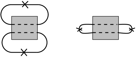
Figure 2: Two of the possible projectors for $\Delta r$. The dashed lines represent the strings of Dirac matrices, while the crosses, the projection operators.

Two possibilities of closing the spinor strings with trace operators are depicted in Fig. 2. The left one has been used in Freitas:2002ja and is given by the equation

$$A=\frac{1}{4d}\int\text{Tr}(\Gamma_{1}\gamma^{\mu}P_{R})\text{Tr}(\Gamma_{2}\gamma_{\mu}P_{R}),$$ (14)

where the dimension of space-time $d$ has been kept arbitrary and the trace of the unit matrix has been put to 4, as usual. A second possibility which we used to perform the calculations presented in this work is given by

$$A=-\frac{1}{2d(d-2)}\int\text{Tr}(\Gamma_{1}\gamma_{\mu}P_{R}\Gamma_{2}\gamma^{\mu}P_{R}),$$ (15)

and corresponds to the right picture in Fig. 2

Both projectors are obviously equivalent in four dimensions due to the Chisholm identity as explained above. The difference starts to be important for divergent integrals. In fact the problem does only occur for one-particle-irreducible four-point diagrams, where the divergence can come from two sources. First from the external wave function renormalisation, which is incomplete due to infrared divergences and second due to infrared divergences of the diagrams themselves. As noticed in Freitas:2002ja the first projector Eq. 14 needs to be corrected, as it does not fulfil several requirements, like for example the vanishing of diagrams with propagator insertion in the photon lines. Moreover, one can explicitely check that without corrections the subtracted diagrams in the Pauli–Villars approach do not cancel and the dependence on the $\Lambda$ scale remains. In the automatic factorisation approach this shows up through an incomplete cancellation of divergences. Notice, however that the result is gauge independent, thus it is only the finiteness of the result that shows that the projector is incorrect.

On the contrary the projector Eq. 15 does not require any corrections. It does fulfil all of the algebraic requirements and also yields a finite result as well as the exact cancellation of the subtraction diagrams of Fig. 1 in $d$-dimensions and in all orders of perturbation theory. This useful property follows from the fact that this projector respects the Fierz symmetry in $d$-dimensions. One can check explicitely that for example

$$\gamma_{\mu}\gamma_{\nu}\gamma_{\rho}P_{L}\otimes\gamma^{\rho}\gamma^{\nu}\gamma^{\mu}P_{L}\sim\gamma_{\mu}\gamma_{\nu}\gamma_{\rho}\gamma^{\nu}\gamma^{\mu}P_{L}\otimes\gamma^{\rho}P_{L},$$ (16)

where $\sim$ means equality after projection.

III On-shell renormalisation

Two-loop calculations within the on-shell renormalisation scheme require the knowledge of several counterterms. At the very least charge and mass counterterms are needed. In this section we first discuss the problem of gauge invariance in connection with tadpole diagrams. We then give specific expressions for the required counterterms.

III.1 Tadpoles and gauge invariance of counterterms

It has been known for a long time that the inclusion of tadpoles is necessary to obtain gauge invariant counterterms. In fact this property has been first noticed Appelquist:ms shortly after the proof of renormalisability of gauge theories. A general proof of the Quantum Action Principle, which has for consequence the gauge invariance of on-shell processes in the bare lagrangian, requires the inclusion of even those tadpoles which would be cancelled by normal ordering (one loop tadpoles) Breitenlohner:hr . There are, however, two disadvantages of using tadpoles in actual calculations. First, this requires the inclusion of diagrams, which drop in the final result. Second, one-particle-irreducible (1PI) Green functions cannot contain tadpoles. As long as we wish to obtain results at the least cost and by using automated software, it is interesting to consider alternative possibilities.

It turns out that it is possible to prepare the bare lagrangian in such a way, that the only gauge dependent quantities would be the wave function renormalisation constants and the vacuum renormalisation constant, and still all of the tadpoles would be cancelled. Let us start by considering a lagrangian in which the bare coupling and masses are defined through physical processes. The masses can be equivalently defined through the position of the poles of the physical $S$-matrix in the complex plane as recently proved Gambino:1999ai . In such a case all of the bare parameters would be gauge invariant, because they would fulfil equations that have this same property. It is important to supply a condition on the vacuum expectation value of the bare Higgs field $v_{0}$ that would resum terms of order ${\cal O}(\alpha^{0})$. A choice which is still consistent with gauge invariance is

$$\frac{1}{2}v_{0}\left(\frac{1}{2}v_{0}^{2}\lambda_{0}-\mu_{0}^{2}\right)=0,$$ (17)

where $\lambda_{0}$ and $\mu_{0}$ are defined through the Higgs lagrangian

$${\cal L}_{\text{Higgs}}=\frac{1}{2}\mu_{0}^{2}\Phi_{0}^{\dagger}\Phi_{0}-\frac{1}{4}\lambda_{0}(\Phi_{0}^{\dagger}\Phi_{0})^{2},$$ (18)

and $\Phi_{0}$ is the Higgs doublet. Eq. 17 implies the vanishing of the linear term in the lagrangian. Although this term will be subsequently altered, the tree level contribution will always vanish.

We now introduce an additional renormalisation of the bare vacuum expectation value

$$v_{0}\longrightarrow v_{0}Z_{v}^{1/2}.$$ (19)

The renormalisation constant $Z_{v}$ can be used to cancel the tadpoles recursively, which implies together with Eq. 17 that the first non-vanishing term in its perturbative expansion starts at order ${\cal O}(\alpha)$. The linear term in the Higgs field can now be written as

$$-T_{0}H^{0}=-\frac{M^{0}_{W}\sin\theta_{W}^{0}}{e_{0}}(M^{0}_{H})^{2}Z_{v}^{1/2}(Z_{v}-1)H^{0}$$ (20)

where the following relations have been used

$$v_{0} = \frac{2\sin\theta_{W}^{0}M_{W}^{0}}{e_{0}},$$ (21)

$$\mu^{2}_{0} = (M_{H}^{0})^{2},$$ (22)

$$\lambda_{0} = \left(\frac{e_{0}M_{H}^{0}}{\sin\theta_{W}^{0}M_{W}^{0}}\right)^{2}.$$ (23)

At the tree level the contribution is zero, since then $Z_{v}^{(0)}=0$, as noticed above. To one-loop order, the relation between the tadpole diagrams and the vacuum expectation value is simple

$$\delta Z_{v}^{(1)}=\frac{e}{\sin\theta_{W}M_{W}M_{H}^{2}}\Pi_{H}^{(1)},$$ (24)

where $i\Pi_{H}^{(1)}$ is the sum of 1PI one-loop tadpole diagrams of the Higgs field. The situation gets much more complicated at the two-loop level

$$\delta Z_{v}^{(2)}=\frac{e}{\sin\theta_{W}M_{W}M_{H}^{2}}\Pi_{H}^{(2)}-\frac{1}{2}\delta Z_{v}^{(1)}\left(\delta Z_{v}^{(1)}+\delta Z_{H}^{(1)}+2\frac{\delta M_{H}^{2(1)}}{M_{H}^{2}}+\frac{\delta M_{W}^{2(1)}}{M_{W}^{2}}+2\frac{\delta\sin\theta_{W}^{(1)}}{\sin\theta_{W}}-\delta Z_{e}^{(1)}\right).$$ (25)

At this level an insertion of this counterterm reproduces all of the tadpole diagrams that would be included in the usual approach. An example is depicted in Fig. 3. An insertion of $Z_{v}$ into the $W$ boson self-energy a), leads effectively through the first term in Eq. 25 to an insertion of a one-loop tadpole with with a vertex counterterm b). This counterterm also contains a correction to the Vacuum expectation value of the Higgs field, which reproduces the tadpole diagram c).

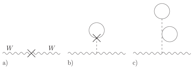
Figure 3: Vacuum expectation value counterterm insertion into the $W$ boson self-energy a), reproducing tadpole insertions b) and c).

III.2 On-shell scheme counterterms

The on-shell renormalisation scheme is defined by the requirement that the masses be identified through the poles of the physical $S$-matrix (as the real part of the pole), while the electric charge coincide with the value measured in the Thompson scattering process as for example in the quantum Hall effect. These conditions are enough to fix all of the free parameters of the SM with minimal Higgs sector (neglecting the CKM matrix and the strong coupling constant). The counterterms have been given by many authors. The peculiarity of the present work is the specific definition of the bare masses which are gauge invariant without including tadpole diagrams. This, however, implies that the formulae defining the counterterms will be slightly different.

At the one-loop level, the mass counterterms are related to the on-shell self-energies through

$$\delta M_{H}^{2(1)} = {\text{Re}}\Pi_{HH}^{(1)}(M_{H}^{2})-\frac{3}{2}M_{H}^{2}\delta Z_{v}^{(1)},$$ (26)

$$\delta M_{W}^{2(1)} = -\Pi_{WW,T}^{(1)}(M_{W}^{2})-M_{W}^{2}\delta Z_{v}^{(1)},$$ (27)

$$\delta M_{Z}^{2(1)} = -\Pi_{ZZ,T}^{(1)}(M_{Z}^{2})-M_{Z}^{2}\delta Z_{v}^{(1)},$$ (28)

where $i\Pi_{ii,T}$ denotes the transverse part of the self-energy diagrams of the boson $i$. For bosonic corrections to the Higgs boson mass counterterm the real part has to be taken due to the possible decay into a $W$ or $Z$ boson pair. To one-loop order this still yields a gauge invariant result for the renormalised amplitude. The $W$ and $Z$ bosons do not require such a treatment neither at one nor at two-loop order.

At the two-loop order, only $W$ and $Z$ boson mass counterterms are needed, and they assume the form

$$\delta M_{W}^{2(2)} = -\Pi_{WW,T}^{(2)}(M_{W}^{2})-\delta Z_{W}^{(1)}\delta M_{W}^{2(1)}-M_{W}^{2}\delta Z_{v}^{(2)}-\delta Z_{v}^{(1)}(M_{W}^{2}\delta Z_{W}^{(1)}+\delta M_{W}^{2(1)}),$$ (29)

$$\delta M_{Z}^{2(2)} = -\Pi_{ZZ,T}^{(2)}(M_{Z}^{2})-\delta Z_{Z}^{(1)}\delta M_{Z}^{2(1)}-M_{Z}^{2}\delta Z_{v}^{(2)}-\delta Z_{v}^{(1)}(M_{Z}^{2}\delta Z_{Z}^{(1)}+\delta M_{Z}^{2(1)})+\frac{1}{4}M_{Z}^{2}(\delta Z_{\gamma Z}^{(1)})^{2}.$$ (30)

The last term in the $Z$ boson mass counterterm, which does not occur in the $W$ boson mass counterterm, has its origin in the mixing between $Z$ and $\gamma$. If the self-energies have imaginary parts, then suitable additional terms have to be included as described in Freitas:2002ja . The above formulae are valid only if the subdivergencies in the two-loop self-energies are renormalised. They also require the wave function renormalisation constants of the bosons

$$\delta Z_{W}^{(1)} = \Pi^{(1)^{\prime}}_{WW,T}(M_{W}^{2}),$$ (31)

$$\delta Z_{Z}^{(1)} = \Pi^{(1)^{\prime}}_{ZZ,T}(M_{Z}^{2}),$$ (32)

and the mixing renormalisation

$$\delta Z_{\gamma Z}^{(1)}=\frac{2}{M_{Z}^{2}}\Pi_{\gamma Z,T}^{(1)}(M_{Z}^{2}).$$ (33)

The last two constants form part of the $2\times 2$ renormalisation matrix of the neutral bosons

$$\left(\begin{array}[]{c}A^{0}_{\mu}\\ Z^{0}_{\mu}\end{array}\right)=\left(\begin{array}[]{cc}Z^{1/2}_{ZZ}&\frac{1}{2}Z_{\gamma Z}\\ \frac{1}{2}Z_{Z\gamma}&Z^{1/2}_{\gamma\gamma}\end{array}\right)\left(\begin{array}[]{c}A_{\mu}\\ Z_{\mu}\end{array}\right).$$ (34)

The remaining two renormalisation constants define the photon field and can be obtained at zero momentum transfer from the following formulae

$$\delta Z^{(1)}_{Z\gamma} = -\frac{2}{M_{Z}^{2}}\Pi^{(1)}_{\gamma Z,T}(0),$$ (35)

$$\delta Z^{(1)}_{\gamma\gamma} = \Pi^{(1)^{\prime}}_{\gamma\gamma,T}(0).$$ (36)

The electric charge counterterm can be obtained in two ways. The first consists in simply calculating the scattering of fermions off real photons, i.e. at zero momentum transfer. This however introduces unnecessarily three point functions. A second possibility is to use the $U(1)$ Ward identity. The suitable relation between the wave function renormalisation constants of the photon and the $Z$ boson has been proved in bauberger:phd using the $BRS$ symmetry. A simpler proof is given in appendix A. The one and two-loop counterterms in the on-shell scheme are given by

$$\delta Z_{e}^{(1)} = -\frac{1}{2}\delta Z^{(1)}_{\gamma\gamma}-\frac{1}{2}\frac{\sin\theta_{W}}{\cos\theta_{W}}\delta Z^{(1)}_{Z\gamma},$$ (37)

$$\delta Z_{e}^{(2)} = -\frac{1}{2}\delta Z^{(2)}_{\gamma\gamma}-\frac{1}{2}\frac{\sin\theta_{W}}{\cos\theta_{W}}\delta Z^{(2)}_{Z\gamma}+(\delta Z_{e}^{(1)})^{2}+\frac{1}{8}(\delta Z^{(1)}_{\gamma\gamma})^{2}-\frac{1}{2}\frac{\delta\sin\theta_{W}}{\cos^{3}\theta_{W}}\delta Z^{(1)}_{Z\gamma}.$$ (38)

The two-loop wave function renormalisation of the photon is given by the short formula

$$\delta Z^{(2)}_{\gamma\gamma}=\Pi^{(2)^{\prime}}_{\gamma\gamma,T}(0)-\frac{1}{4}(\delta Z^{(1)}_{Z\gamma})^{2},$$ (39)

whereas in the mixing counterterm, the vacuum expectation value correction makes again its appearance

$$\delta Z^{(2)}_{Z\gamma}=-\frac{2}{M_{Z}^{2}}\Pi^{(2)}_{\gamma Z}(0)-\frac{1}{2}\delta Z^{(1)}_{ZZ}\delta Z^{(1)}_{Z\gamma}-\frac{1}{M_{Z}^{2}}\delta Z^{(1)}_{Z\gamma}\delta M_{Z}^{2(1)}-\delta Z^{(1)}_{v}\delta Z^{(1)}_{Z\gamma}.$$ (40)

In the on-shell calculation the ghost sector was also renormalised. The respective constants are as in Freitas:2002ja up to an unimportant renormalisation of the ghost wave functions, the difference being dictated by simplicity. The wave function renormalisation constants of the ghosts and Goldstone bosons have been left unspecified. For the ghosts, these constants cancel trivially within every closed loop. With the Goldstone bosons, the situation is more complicated, since the fact that the gauge fixing term should not be renormalised induces Goldstone wave function renormalisation constants in the ghost sector. These can only cancel in gauge invariant quantities. This indeed happened for all the mass and coupling counterterms and for the complete result.

IV $\overline{\text{MS}}$ renormalisation

In this section we describe in detail the renormalisation of $\Delta r$ in the $\overline{\text{MS}}$ scheme. $\Delta r$ is computed through the matching procedure described before in Section II. Here we chose the strategy of multiplicative renormalisation. After multiplication by the on-shell wave function renormalisation constants of external fermion fields, the result is expressed in terms of bare masses and bare electric charge. In order to get the $\overline{\text{MS}}$ renormalised result for $G_{F}$ one needs to substitute all bare parameters in the form

$$e_{0} = \mu^{\varepsilon}\,Z_{e}\,e(\mu),$$

$$(m_{i}^{0})^{2} = Z_{m_{i}}m^{2}_{i}(\mu),$$ (41)

where $e(\mu)$ and $m_{i}(\mu)$ are the $\overline{\text{MS}}$ charge and masses respectively and $\mu$ is the $\overline{\text{MS}}$ parameter. The $\overline{\text{MS}}$ renormalisation constants will be specified in the next two subsections.

Let us stress that in Eq. 41 we renormalise only the physical parameters and no renormalisation of the unphysical sector (ghost sector and gauge fixing parameters) is required. The renormalisation of the boson particles’ wave functions is also not needed since it cancels anyway in the final expression.

A few words should also be said about tadpole diagrams, which should be added in a proper way in order to obtain a gauge invariant result in the SM. Unlike in the approach described in the Section III.1, where the new counterterm $Z_{v}$ for the Higgs VEV has been introduced, here we include the tadpole diagrams explicitely. This makes our renormalisation constants $Z$’s from Eq. 41 gauge invariant.

Below we present the analytical expressions for charge and mass $\overline{\text{MS}}$ renormalisation constants, needed in order to obtain a finite expression for $\Delta r$ in the $\overline{\text{MS}}$ scheme.

IV.1 Coupling and masses renormalisation

The bare charge $e_{0}$ and the $\overline{\text{MS}}$ charge $e$ are related via

$$e_{0}=\mu^{\varepsilon}e\>\left(1+\frac{e^{2}(\mu)}{16\pi^{2}\varepsilon}Z_{e}^{(1,1)}+\frac{e^{4}(\mu)}{(16\pi^{2})^{2}\varepsilon}Z_{e}^{(2,1)}+\frac{e^{4}(\mu)}{(16\pi^{2})^{2}\varepsilon^{2}}Z_{e}^{(2,2)}\right)\,,$$ (42)

where the constants $Z$’s, as we shall see in the following, can depend on $\sin\theta_{W}$.

There are two ways to determine the $\overline{\text{MS}}$ renormalisation constant in this expression. One is to use the Ward–Takahashi identity given in appendix A to express it in terms of the gauge boson wave function renormalisation constants and the renormalisation constant for $\sin\theta_{W}$

$$1=Z_{e}\left\{\sqrt{Z_{\gamma\gamma}}+\frac{1}{2}\frac{\sin\theta_{W}^{0}}{\cos\theta_{W}^{0}}\delta Z_{Z\gamma}\right\}.$$ (43)

Then at the one- and two-loop order for on-shell charge renormalisation constants, introduced above, we have

$$\delta Z_{e,\rm OS}^{(1)} = -\frac{1}{2}\delta Z_{\gamma\gamma}^{(1)}-\frac{1}{2}\delta Z_{Z\gamma}^{(1)}\frac{\sin\theta_{W}}{\cos\theta_{W}},$$ (44)

$$\delta Z_{e,\rm OS}^{(2)} = -\frac{1}{2}\delta Z_{\gamma\gamma}^{(2)}-\frac{1}{2}\frac{\sin\theta_{W}^{0}}{\cos\theta_{W}^{0}}\delta Z_{Z\gamma}^{(2)}+\left(\delta Z_{e,\rm OS}^{(1)}\right)^{2}+\frac{1}{8}\left(\delta Z_{\gamma\gamma}^{(1)}\right)^{2}.$$ (45)

Here $\delta Z^{(1,2)}$ are one- and two-loop on-shell field renormalisation constants, expressed via bare quantities. We can rewrite $\delta Z^{(2)}_{\gamma\gamma}$ and $\delta Z^{(2)}_{Z\gamma}$ in terms of self-energy diagrams

$$\delta Z_{\gamma\gamma}^{(2)} = \Pi_{\gamma\gamma,T}^{(2)^{\prime}}(0)+\delta Z_{\gamma\gamma}^{(1)}\Pi_{\gamma\gamma,T}^{(1)^{\prime}}(0)+\delta Z_{Z\gamma}^{(1)}\Pi_{\gamma Z,T}^{(1)^{\prime}}(0)-\frac{1}{4}\left(\delta Z_{Z\gamma}^{(1)}\right),$$

$$\delta Z_{Z\gamma}^{(2)} = -\frac{2}{M_{Z}^{2}}\left(\Pi_{\gamma Z,T}^{(2)}(0)+\frac{1}{2}\delta Z_{Z\gamma}^{(1)}\Pi_{ZZ,T}^{(1)}(0)+\frac{1}{2}\delta Z_{\gamma\gamma}^{(1)}\Pi_{\gamma Z,T}^{(1)}(0)+\frac{1}{2}\delta Z_{ZZ}^{(1)}\Pi_{\gamma Z,T}^{(1)}(0)\right)-\frac{1}{2}\delta Z_{ZZ}^{(1)}\delta Z_{Z\gamma}^{(1)},$$ (46)

where this time all of the self energies are unrenormalised. All other one-loop field renormalisation constants were defined before in Section III.2. At the end we have an expression for the on-shell charge renormalisation constant expressed via bare charge, Weinberg angle and masses. Now, rewriting the bare quantities in terms of $\overline{\text{MS}}$ ones with yet unknown coefficients in Eq. 42 and requiring that transition between on-shell and $\overline{\text{MS}}$ charge should not contain divergencies we easily extract the $\overline{\text{MS}}$ charge renormalisation constants.

Alternatively, the renormalisation group analysis can be applied. In order to find $Z_{e}$ we differentiate Eq. (42) w.r.t. $\log\mu^{2}$ and take into account that

$$\frac{d\,e}{d\,\log\mu^{2}}=-\frac{\varepsilon}{2}e+\beta_{e}\,,$$ (47)

where

$$\beta_{e}=\frac{e^{3}}{16\pi^{2}}b_{1}+\frac{e^{5}}{(16\pi^{2})^{2}}b_{1}+\dots$$ (48)

is the $\beta$-function. Since $(d/d\log\mu^{2})\,e_{0}=0$, the l.h.s. of Eq. 42 becomes zero after the differentiation, while the r.h.s. relates the coefficients $b_{j}$ and the unknown constants in (42)

$$Z^{(1,1)}_{e} = b_{0},$$

$$Z^{(2,2)}_{e} = \frac{3}{2}\,b_{0}^{2},$$

$$Z^{(2,1)}_{e} = \frac{1}{2}\,b_{1}\,.$$ (49)

The function $\beta_{e}$ can be extracted from the existing calculation in the unbroken theory. Namely, for the $SU(2)$ and $U(1)$ charges $g$ and $g^{\prime}$ respectively, the $\beta$-functions read

$$\beta_{g^{\prime}} = \frac{1}{12}\frac{g^{\prime 3}}{16\pi^{2}}+\frac{1}{4}\frac{g^{\prime 5}}{(16\pi^{2})^{2}}+\frac{3}{4}\frac{g^{\prime 3}g^{2}}{(16\pi^{2})^{2}}\;\>,$$

$$\beta_{g} = -\frac{43}{12}\frac{g^{3}}{16\pi^{2}}-\frac{259}{12}\frac{g^{5}}{(16\pi^{2})^{2}}+\frac{1}{4}\frac{g^{3}g^{\prime 2}}{(16\pi^{2})^{2}}\;\>.$$ (50)

The one-loop result is given in RG_1loop , while the two-loop coefficients have been evaluated in RG_2loop .

From the relation

$$\frac{1}{e^{2}}=\frac{1}{g^{2}}+\frac{1}{g^{\prime 2}}\;,$$ (51)

it is easy to deduce that

$$\beta_{e}=e^{3}\left(\frac{\beta_{g}}{g^{3}}+\frac{\beta_{g^{\prime}}}{g^{\prime 3}}\right)\,.$$ (52)

Using now Eqs. 50, 51 and 52 we obtain

$$\beta_{e}=-\frac{7}{2}\frac{e^{3}}{16\pi^{2}}+\frac{e^{5}}{(16\pi^{2})^{2}}\left(-\frac{125}{6\sin^{2}\theta_{W}}+\frac{1}{2\cos^{2}\theta_{W}}\right),$$ (53)

and, finally, from Eq. 49 we have

$$Z_{e}^{(1,1)} = -\frac{7}{2},$$

$$Z_{e}^{(2,2)} = \frac{147}{8},$$

$$Z_{e}^{(2,1)} = -\frac{125}{12}\frac{1}{{\rm sin}^{2}\theta_{W}}+\frac{1}{4}\frac{1}{{\rm cos}^{2}\theta_{W}}.$$ (54)

The explicit calculation confirms the above result.

Similarly to the charge renormalisation we write for the masses of the $Z$, $W$ and the Higgs bosons

$$(m^{0}_{V})^{2}=m_{V}^{2}(\mu)\>\left(1+\frac{g^{2}(\mu)}{16\pi^{2}\varepsilon}Z_{V}^{(1,1)}+\frac{g^{4}(\mu)}{(16\pi^{2})^{2}\varepsilon}Z_{V}^{(2,1)}+\frac{g^{4}(\mu)}{(16\pi^{2})^{2}\varepsilon^{2}}Z_{V}^{(2,2)}\right).$$ (55)

For $m_{Z}$ and $m_{W}$ the renormalisation constants up to two loop are required while for the Higgs boson we need only the one loop expression. The analysis, similar to that described above for the charge, has been done in details in olegmisha . There the explicit expressions for $Z_{V}^{(1,1)}$, $Z_{V}^{(2,1)}$ and $Z_{V}^{(2,2)}$ are given.

IV.2 $\overline{\text{MS}}$ results for $\Delta r$

In Fig. 4 we plot $\Delta r^{(2)\overline{\rm MS}}_{\rm bos}$ as a function of the $\overline{\text{MS}}$ Higgs boson mass in different scales. As input parameters we used the on-shell values given in Table I.

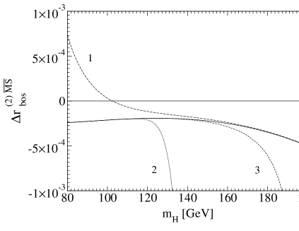
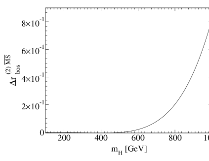
Figure 4: The exact result (solid line) for the $\Delta r^{(2)}_{\rm bos}$ in the in the $\overline{\text{MS}}$ scheme (left and right panel) vs. its 1) large Higgs boson mass expansion (long dashed line) and 2) mass difference expansion (dotted line). The short dashed line 3) represents the [3/3] Padé approximant. In the right pannel the large Higgs boson mass expansion curve coincides completely with the numerical result for this range.

The solid curve represents the exact result. Two other curves represent expansions in different regimes: as $m_{H}\to m_{Z}$ and as $m_{H}\to\infty$. They cover almost the whole region of the $m_{H}$ under consideration. In order to extend the range of the expansion around $m_{Z}$ the Padé approximant has been constructed. It sufficiently improves the situation for the intermediate Higgs boson masses. Thus the expansions cover completely the region of interest. The details of expansions are discussed more precisely in Section VI.2.

V Transition between the schemes

Once we have the result in the $\overline{\text{MS}}$ scheme it is necessary to translate it into the on-shell parameters, which are known with high precision for the electroweak sector contrary to the strong interacting sector of the Standard Model. To this end one has to consider the proper scheme independent quantity which is

$$\frac{\alpha\pi}{2M_{W}^{2}\sin^{2}\theta_{W}}(1+\Delta r)\equiv\frac{G_{F}}{\sqrt{2}}.$$ (56)

This should be contrasted with the naive approach of taking simply $\Delta r$ and substituting $\overline{\text{MS}}$ parameters.

Using the methods described in Section IV, we obtain the following series expansions connecting on-shell and $\overline{\text{MS}}$ parameters

$$\alpha_{\text{OS}} = \alpha_{\overline{\text{MS}}}\left(1+\frac{\alpha_{\overline{\text{MS}}}}{4\pi}x^{\alpha}_{1,\overline{\text{MS}}}+\left(\frac{\alpha_{\overline{\text{MS}}}}{4\pi}\right)^{2}x^{\alpha}_{2,\overline{\text{MS}}}\right),$$ (57)

$$M_{W,\text{OS}}^{2} = M_{W,\overline{\text{MS}}}^{2}\left(1+\frac{\alpha_{\overline{\text{MS}}}}{4\pi}x^{W}_{1,\overline{\text{MS}}}+\left(\frac{\alpha_{\overline{\text{MS}}}}{4\pi}\right)^{2}x^{W}_{2,\overline{\text{MS}}}\right),$$ (58)

$$M_{Z,\text{OS}}^{2} = M_{Z,\overline{\text{MS}}}^{2}\left(1+\frac{\alpha_{\overline{\text{MS}}}}{4\pi}x^{Z}_{1,\overline{\text{MS}}}+\left(\frac{\alpha_{\overline{\text{MS}}}}{4\pi}\right)^{2}x^{Z}_{2,\overline{\text{MS}}}\right),$$ (59)

$$M_{H,\text{OS}}^{2} = M_{H,\overline{\text{MS}}}^{2}\left(1+\frac{\alpha_{\overline{\text{MS}}}}{4\pi}x^{H}_{1,\overline{\text{MS}}}\right).$$ (60)

The series for the Higgs boson mass relation is only needed to first order, since the Higgs field starts to contribute to the decay only at the one-loop level.

The above relations have to be inverted to yield $\overline{\text{MS}}$ parameters in terms of the on-shell ones. For any parameter $A$ the relation will be written as follows

$$A_{\overline{\text{MS}}}=A_{\text{OS}}\left(1+\frac{\alpha_{\text{OS}}}{4\pi}X^{A}_{1,\text{OS}}+\left(\frac{\alpha_{\text{OS}}}{4\pi}\right)^{2}X^{A}_{2,\text{OS}}\right).$$ (61)

The expansion coefficients are obtained by inverting the original series up to the required order. At one-loop this leads trivially to

$$X^{A}_{1,\text{OS}}=\left[-x^{A}_{1,\overline{\text{MS}}}\;\;\right]_{M_{i,\overline{\text{MS}}}\;\rightarrow\;M_{i,\text{OS}}}.$$ (62)

The coefficients for the three bosons are depicted in Fig. 5 with parameters values as given in Table 1, in a comparison of the different evaluation methods. For Higgs boson masses greater than 200 GeV the large mass expansion with six coefficients is indiscernible from the numeric result. The mass difference expansion fails always around 120 GeV. In the visible range from 80 GeV to 200 GeV, the Padé approximation based on the mass difference expansion turns out to practically coincide with the exact result for the vector bosons. For the Higgs boson this cannot happen due to the occurrence of the two-particle production thresholds and indeed there is a region between the thresholds which cannot be reproduced with neither the mass difference nor the large mass expansion. Obviously if it was needed this region could be covered by threshold expansions.

$\alpha^{-1}$	137.03599976(50)
$M_{W}$	80.423(39) GeV
$M_{Z}$	91.1876(21) GeV

Table 1: Parameter values used in the calculation Hagiwara:pw .

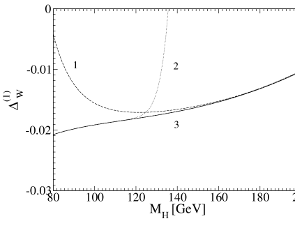
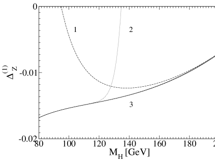
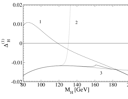
Figure 5: One-loop corrections to the relations between the on-shell and the $\overline{\text{MS}}$ masses for the $W$, $Z$ and Higgs bosons ($\Delta^{1}_{i}=\alpha/(4\pi)X^{i}_{1}$). The long dashed line 1) represents the large Higgs boson mass expansion, the dotted line 2) represents the mass difference expansion. The short dashed line 3) gives the [4/4] Padé approximant which coincides for this range with the exact result for the $W$ and $Z$ boson mass corrections.

The two-loop correction contains terms coming also from the one-loop terms and the proper expression reads

$$X^{A}_{2,\text{OS}}=\left[-x^{A}_{2,\overline{\text{MS}}}+x^{\alpha}_{1,\overline{\text{MS}}}x^{A}_{1,\overline{\text{MS}}}+\sum_{i}M^{2}_{i,\overline{\text{MS}}}\frac{\partial x^{A}_{1,\overline{\text{MS}}}}{\partial M^{2}_{i,\overline{\text{MS}}}}x^{i}_{1,\overline{\text{MS}}}\;\;\right]_{M_{i,\overline{\text{MS}}}\;\rightarrow\;M_{i,\text{OS}}}.$$ (63)

The corrections for the vector bosons are depicted similarly to the one-loop case in Fig. 6. The expansions themselves are less precise. It is however interesting to note that the Padé approximation together with the large mass expansion cover the whole range with high precision. Even the threshold region is reproduced with a relatively small error, although this is due to the fact that the peaks are not very pronounced.

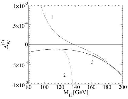
Figure 6: Two-loop corrections to the relation between the on-shell and the $\overline{\text{MS}}$ masses for the $W$ and $Z$ boson ($\Delta^{2}_{i}=(\alpha/(4\pi))^{2}X^{i}_{2}$). The long dashed line 1) represents the large Higgs boson mass expansion, the dotted line 2) represents the mass difference expansion. The short dashed line 3) gives the [4/4] Padé approximant.

We can now combine all the perturbative expansions and translate the $\overline{\text{MS}}$ result into the on-shell one. We shall not reproduce the formula since it can be easily obtained from the previous equations. It is important however to note two things. First, in the expression for the two-loop $\Delta r$ there are the following terms

$$\left(\Delta r^{(2)}\right)^{\text{OS}}=\dots+\frac{X^{W}_{2,\text{OS}}}{\sin^{2}\theta_{W}}-\frac{X^{Z}_{2,\text{OS}}}{\sin^{2}\theta_{W}}+\dots$$ (64)

If this is combined with the fact that the results in both $\overline{\text{MS}}$ and on-shell schemes behave as $1/\sin^{4}\theta_{W}$, it is obvious that one term in the $W$ and $Z$ boson mass difference expansion is lost. Second, the result in the $\overline{\text{MS}}$ scheme behaves as $M_{H}^{4}$, whereas the one in the on-shell scheme as $M_{H}^{2}$. Therefore, one term in large Higgs boson mass expansion is also lost. As a result, if the expansions of olegmisha are taken, the final result can be given with five coefficients in both expansions in the large mass case. The formulae can be found in Appendix B. The mass difference expansion requires an independent calculation of the on-shell propagator diagrams and the result can be found in Appendix C. The numeric results can be found in Fig. 7. It should be stressed, that it was checked that the exact analytic result without expansions obtained by the translation procedure described above and by an explicit renormalisation in the on-shell scheme are the same.

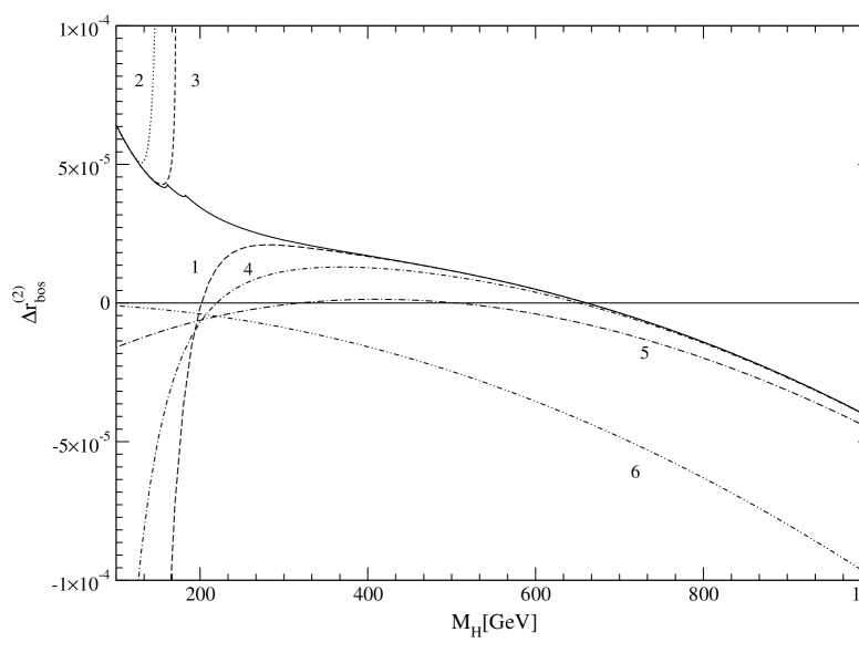
Figure 7: On-shell $\Delta r^{(2)}_{\rm bos}$. The long dashed line 1) represents the large Higgs boson mass expansion, the dotted line 2) represents mass difference expansion. The short dashed line 3) gives the [3/3] Padé approximant. The dash-dotted 4) and 5) lines correspond to lower terms in the large Higgs boson mass expansion, whereas 6) is the leading term.

It is interesting to consider the transition between the schemes performed purely numerically. In Fig. 8, the solid curve represents the one-loop correction as well as the sum of the one- and two-loop corrections. The fact that they are indiscernible in this scale is due to their relative smallness. The most reliable way of obtaining the correction (apart from the exact method) is to take the one-loop result and substitute the $\overline{\text{MS}}$ parameters only in the normalisation in Eq. 56, whereas the masses in $(\Delta r^{(1)}_{\text{bos}})^{\overline{\text{MS}}}$ should be left in the on-shell scheme. This is shown in the curve 2). If one, however, simply takes the whole invariant and substitutes all of the $\overline{\text{MS}}$ parameters, then curve 1) is obtained, which diverges strongly for Higgs boson masses larger than about 250 GeV. It turns out that the sum of the one- and two-loop corrections does not reduce substantially the scheme dependence, as shown by curve 3), where the correction up to two-loop order in the $\overline{\text{MS}}$ scheme has been given for $\overline{\text{MS}}$ parameters translated from on-shell values using Eqs. 57 to 60.

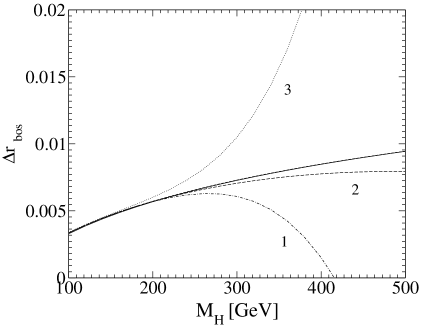
Figure 8: Numeric translation of $\Delta r$ form the $\overline{\text{MS}}$ scheme to the on-shell scheme vs. the exact result (solid line).

VI Computational methods

The calculation of the bosonic corrections to the muon life time is a relatively complex task. The number of Feynman diagrams to be calculated is around 5000 in $R_{\xi}$ gauge. This makes it necessary to use automated software.

VI.1 Software and checks

The first step of the calculation is the generation of diagrams. Several systems are presently available. Obviously each differs in its easy of use, speed and design concepts.

The on-shell calculation was based on the C++ library DiaGen diagen . It generates all diagrams together with all necessary counterterms. The main advantage of this software is the speed, since all of the diagrams were generated in a few seconds, thus making the generation phase a negligible part of the calculation.

Alternatively, for the calculation with the tadpoles the input generator DIANA DIANA has been applied. We note that according to the rules, given in Section IV, no counterterm diagrams should be generated. They are all taken into account by the multiplicative renormalisation.

The diagrams to be evaluated can be divided into two broad classes. First are these which can be reduced to vacuum bubbles. Here, partial integration identities Chetyrkin:qh supplied with analytical formulae Davydychev:1992mt can be used.

The second more complicated problem is the evaluation of the two-loop two-point functions at non-vanishing external momentum (at the values $q^{2}=M_{Z}^{2}$ and $q^{2}=M_{W}^{2}$ in our case). From the several possibilities two different algorithms have been used to deal with these diagrams.

The algorithm described in Weiglein:hd has been chosen because of its simplicity. As an end result of the tensor reduction scalar two-loop propagator integrals are obtained. A high precision numerical evaluation of these is currently possible with one dimensional integral representations Bauberger:1994hx . To this end C++ programs were used based on the library S2LSE s2lse . For large scale differences which occur when the Higgs mass is much above the masses of the $W$ and the $Z$ boson double precision turns out to be insufficient. An easy way to see it is to remark that the individual terms in the result can behave as $M_{H}^{8}$ whereas due to the screening theorem Veltman:1976rt the whole result behaves at most as $M_{H}^{2}$. For a Higgs boson mass of the order of 1 TeV, this means that cancellations of the order of $10^{6}$ will have to occur. If we combine this with the fact that in double precision some of the integrals can only be evaluated to 5 digits, the numerical instability becomes apparent. A way out of this problem on 32 bit machines is to use software emulated quadruple precision. Of course this signifies an important drop in effectiveness. In practice, the software runs about 20 times slower. Ten times are due to the use of software emulation for arithmetical operations and two to more integration points which are needed for higher precision. On present GHz processors, the evaluation of a single point of the final result requires around 20s and a conservative estimate of the error over the whole range of Higgs boson mass from 100 GeV to 1 TeV is four digits.

Alternatively to the numerical method, we used also the semianalytic method of expansions (see next subsection). In this case the huge cancellations mentioned above do not cause any problem.

The size of the programs written in C++ and in FORM Vermaseren:2000nd requires stringent checks. A helpful property of the bosonic corrections to the propagators is that the value of every single diagram can be obtained rather easily through low momentum or large mass expansions. In fact for the $Z$ boson propagators a low momentum expansion up to tenth order provided a five digit agreement with the integral representations for each diagram independently and for the whole sum. Additionally, we also made an expansion around the point $M_{H}=M_{Z}$ (see next subsection) and got excellent agreement between the numerical and the expanded results. In the case of the $W$ boson propagators not all of the diagrams are below threshold. It turns out that 345 contain a photon or a massless ghost line, which makes as much as around 160 of them to be either on threshold or infrared divergent. In this case the low momentum expansion either fails to converge or converges very slowly. A way out of this is given by large mass expansions. If the lines which are to be considered as heavy are chosen in a specific way, then the large mass expansion leads only to vacuum bubbles and one-loop propagator diagrams and the convergence is comparable to the case of the $Z$ boson propagators. An example choice of the heavy lines for two different topologies is given in Fig. 9. This procedure fails only for graphs which represent pure $QED$ corrections to a $W$ boson line. In this case however, the result is known analytically Gray:1990yh .

Figure 9: A choice of formally heavy lines in the large mass expansion of two $W$ boson propagator topologies.

Another way of testing the analytical reduction and the diagram generation software is to check the Ward–Takahashi identities for the propagators. Here the following relations have been evaluated

$$p^{2}\left(\Pi^{(2)}_{ZZ,L}+2iM_{Z}\Pi^{(2)}_{ZG_{Z}}\right)+M_{Z}^{2}\Pi^{(2)}_{G_{Z}G_{Z}}-p^{2}\left(\Pi^{(1)}_{ZG_{Z}}\right)^{2}+\Pi^{(1)}_{ZZ,L}\Pi^{(1)}_{G_{Z}G_{Z}} = 0,$$ (65)

$$p^{2}\left(\Pi^{(2)}_{WW,L}-2M_{W}\Pi^{(2)}_{WG_{W}}\right)+M_{W}^{2}\Pi^{(2)}_{G_{W}G_{W}}-p^{2}\left(\Pi^{(1)}_{WG_{W}}\right)^{2}+\Pi^{(1)}_{WW,L}\Pi^{(1)}_{G_{W}G_{W}} = 0$$ (66)

both for on-shell values of the momentum and in an expansion around zero up to third order. Here $G_{Z}$ and $G_{W}$ stand for the neutral and charged would-be Goldstone boson respectively and the subscript “$L$” denotes longitudinal parts of the vector boson self-energies and the scalar vector transitions are given by

$$\Pi_{VG_{V}}^{\mu}(p)=p^{\mu}\Pi_{VG_{V}}(p^{2}),$$ (67)

where $p$ is the ingoing momentum of the vector boson.

The combination of the two checks described above, tests the software from the diagram generation to the numerical evaluation. An additional test is of course provided by gauge invariance and indeed the calculation was performed in the general $R_{\xi}$ gauge with three independent gauge parameters. We have observed explicitely the cancellation of each of them from the final result and the counterterms.

Since the bosonic corrections to the propagators in the $\overline{\text{MS}}$ scheme have been evaluated within the large Higgs boson mass approach in olegmisha a comparison was also possible for the whole result. It turns out that the agreement is perfect for Higgs masses running as low as 200 GeV.

To complete the description of the computational methods, let us note that C++ and FORM were supplied with a collection of AWK and Bourne shell scripts managed by several Makefiles. The system prepared in this way runs completely automatically from the beginning with diagram generation up to the numerical evaluation with plots. Actually, the specificity of the problem allowed to reduce the evaluation time of the whole problem down to only one hour and a half, which is rather short for multiloop calculations.

VI.2 Expansions

Here we give more details on how the expansions are performed in two different regimes that we considered

• in the mass difference $h_{Z}=(M_{H}^{2}-M_{Z}^{2})/M_{Z}^{2}$ and

• in the mass ratio $z_{H}=M_{Z}^{2}/M_{H}^{2}$.

The expansion in the mass difference $M_{H}^{2}-M_{Z}^{2}$ is especially simple. It is just a Taylor expansion of all Higgs propagators and Higgs boson masses in the vertices around $M_{Z}$. No additional subgraphs are necessary in this case. The expansion in the heavy Higgs boson limit is somewhat more involved. It is given by the rules of asymptotic expansions asymptotic .

In addition in the presence of both $M_{Z}$ and $M_{W}$ we expand in the difference of these masses as well. Indeed

$$\frac{M_{Z}^{2}-M_{W}^{2}}{M_{Z}^{2}}=\sin^{2}\theta_{W}\approx 0.23,$$ (68)

is a rather small parameter and the convergence of this series is quite fast. This trick was used previously in olegmisha . The advantage of this approach is that in the case of on-shell Green functions all integrals have only one scale. This allows one to use the FORM package ONSHELL2 ONSHELL2 to evaluate these integrals analytically.

We should also note that to extend the range of the $h_{Z}$ expansion we apply the Padé approximation. Throughout this paper we use a [3/3] Padé approximant for $\Delta r$ and [4/4] for the scheme transition formulae. The Padé approximation for the $z_{H}$ series does not work well since this series is nonalternating.

VII Conclusions

The recent calculation of the two-loop bosonic corrections to $\Delta r$ performed by two independent groups has been described in detail, from the matching onto the Fermi theory to the renormalisation and the explicit results in the on-shell and $\overline{\text{MS}}$ schemes. The framework for the evaluation of the Fermi constant $G_{F}$ based on the low energy factorisation theorem has been constructed. It allows one to compute $G_{F}$ as a Wilson coefficient in a simple manner. This approach is general and is also applicable to other low energy quantities.

A comparison of different expansions and numerical methods has been given. It has been proven that in the wide range of Higgs boson masses expansions provide as much precision as needed and cover the whole region of interest. The only problematic region, however, is connected to the thresholds for $W$ and $Z$ boson pair production. If the Higgs boson was indeed found in this range, then a precise result could also be obtained with expansions but this time of the threshold type. The coincidence of the numerical and analytical results serves as a strong check of the calculation.

The accuracy of the numerical transformation between $\overline{\text{MS}}$ and on-schemes has been tested. It is shown that for the Higgs boson masses larger than $\sim 250$ GeV the two loop correction does not reduce the scheme dependence which can be explained by huge cancelations of large terms during the transition procedure.

VIII Acknowledgments

The authors would like to thank K. Chetyrkin for fruitful discussions. A. O and O. V. thank M. Tentyukov for his help with DIANA. M. A. would like to thank the “Marie Curie Programme” of the European Commission for a stipend. M. C. would like to thank the Alexander von Humboldt foundation for fellowship. This work was supported in part by the European Community’s Human Potential Programme under contract HPRN-CT-2000-00149 Physics at Colliders, by the KBN Grant 5P03B09320, by DFG-Forschergruppe “Quantenfeldtheorie, Computeralgebra und
Monte-Carlo-Simulation” (contract FOR 264/2-1) and by BMBF under grant No 05HT9VKB0.

Appendix A $U(1)$ Ward identity and the renormalisation of charge

In this appendix we present a derivation of the relation between the charge renormalization constant and different wave function renormalization constants valid to all orders of perturbation theory. The derivation is based on the use of the $U(1)$ Ward–Takahashi identity for the weak hypercharge gauge group. To begin with, let us take the bare $U(1)$ gauge boson field $B_{\mu}^{0}$ and rewrite it in terms of mass eigenstates

$$B_{\mu}^{0}=c_{W}^{0}A_{\mu}^{0}+s_{W}^{0}Z_{\mu}^{0}.$$ (69)

Here $c_{W}^{0}=\cos\theta_{W}^{0}$ and $s_{W}^{0}=\sin\theta_{W}^{0}$ are bare values of cosine and sine of Weinberg angle.

In the next step we express our bare gauge boson fields through the renormalized ones

$$\left(Z_{2}^{B}\right)^{1/2}\left\{c_{W}A_{\mu}+s_{W}Z_{\mu}\right\}=c_{W}^{0}\left\{\frac{1}{2}Z_{\gamma Z}Z_{\mu}+\left(Z_{\gamma\gamma}\right)^{1/2}A_{\mu}\right\}+s_{W}^{0}\left\{\left(Z_{ZZ}\right)^{1/2}Z_{\mu}+\frac{1}{2}Z_{Z\gamma}A_{\mu}\right\}.$$ (70)

Now taking the coefficient in front of $A_{\mu}$ in the equation above we have

$$\left(Z_{2}^{B}\right)^{1/2}c_{W}=c_{W}^{0}\left(Z_{\gamma\gamma}\right)^{1/2}+\frac{1}{2}s_{W}^{0}Z_{Z\gamma}.$$ (71)

To complete the derivation we need to relate the $Z_{2}^{B}$ renormalisation constant to the charge renormalization constant. The electric charge is related to the weak hypercharge via the following equation

$$e^{0}=g_{1}^{0}c_{W}^{0}=\left(Z_{2}^{B}\right)^{-1/2}g_{1}c_{W}^{0}=Z_{e}e=Z_{e}g_{1}c_{W},$$ (72)

where we have made use of $U(1)$ Ward–Takahashi identity $Z_{g_{1}}=\left(Z_{2}^{B}\right)^{-1/2}$. Now we can easily deduce, that

$$Z_{e}=\left(Z_{2}^{B}\right)^{-1/2}\frac{c_{W}^{0}}{c_{W}}.$$ (73)

Substituting this relation into Eq. 71 we have

$$1=Z_{e}\left\{\left(Z_{\gamma\gamma}\right)^{1/2}+\frac{s_{W}^{0}}{c_{W}^{0}}\frac{1}{2}Z_{Z\gamma}\right\}.$$ (74)

Using this final relation one can considerably simplify the calculation of the on-shell charge renormalization constant and avoid dealing with infrared rearrangement while computing the three-point Green function.

Appendix B Large Higgs boson mass expansion of $\Delta r^{(2)}_{\text{bos}}$ in the on-shell scheme

In this appendix, the on-shell renormalised $\Delta r^{(2)}_{\text{bos}}$ is given in a twofold expansion, in the large Higgs boson mass and in the mass difference between the $W$ and the $Z$ boson. The number of terms is consistent with the result olegmisha as explained in Section V. The leading behaviour both in the Higgs mass and in the sine of the Weinberg angle has been factorised out.

$$\left(\Delta r^{(2)}_{\text{bos}}\right)^{\text{OS}}=\left(\frac{\alpha}{4\pi\sin^{2}\theta_{W}}\right)^{2}\frac{M_{H}^{2}}{M_{Z}^{2}}\sum^{4}_{n=0}\sin^{2n}\theta_{W}R^{\text{OS}}_{n}.$$ (75)

The occurring transcendental numbers are

$$S_{1} = \frac{\pi}{\sqrt{3}},$$ (76)

$$S_{2} = \frac{4}{9}\frac{\text{Cl}_{2}(\pi/3)}{\sqrt{3}}\simeq 0.2604341376321620989557291432080308...$$

while $z_{H}=M_{Z}^{2}/M_{H}^{2}$. Note that the leading term in the Higgs boson mass can be resumed in $\sin^{2}\theta_{W}$ to give the behaviour

$$\Delta r^{(2)}_{\text{Higgs}}=\left(\frac{\alpha}{4\pi\sin^{2}\theta_{W}}\right)^{2}\frac{M_{H}^{2}}{8M_{W}^{2}}\left(9\sqrt{3}\mbox{ Cl}_{2}(\frac{\pi}{3})+\frac{49}{72}-\frac{11\pi\sqrt{3}}{4}-\frac{25\pi^{2}}{108}\right).$$ (77)

The expansion coefficients read (the first four of them expanded to the order $O(z_{H}^{3})$ were already published in oni )

$$R^{\text{OS}}_{0}= \Biggl{[}-{\textstyle{\frac{33}{32}}}\,S_{1}-{\textstyle{\frac{25}{144}}}\,\zeta_{2}+{\textstyle{\frac{49}{576}}}+{\textstyle{\frac{243}{32}}}\,S_{2}\Biggr{]}$$

$$+ z_{H}\,\Biggl{[}-{\textstyle{\frac{303659}{384}}}\,S_{1}-{\textstyle{\frac{1515}{16}}}\,\zeta_{3}-{\textstyle{\frac{125}{4}}}\,\text{ln}(z_{H})\,S_{1}+{\textstyle{\frac{41}{288}}}\,\text{ln}(z_{H})^{2}+{\textstyle{\frac{17305}{576}}}\,\zeta_{2}+{\textstyle{\frac{98125}{1728}}}\,\text{ln}(z_{H})+{\textstyle{\frac{4131}{32}}}\,S_{1}\,S_{2}$$

$$+{\textstyle{\frac{1089}{8}}}\,S_{1}^{2}+{\textstyle{\frac{7069829}{20736}}}+{\textstyle{\frac{259443}{128}}}\,S_{2}+66\,\text{ln}(3)\,\zeta_{2}\Biggr{]}$$

$$+ z_{H}^{2}\,\Biggl{[}-{\textstyle{\frac{75341}{960}}}\,S_{1}-{\textstyle{\frac{41441}{1440}}}\,\zeta_{2}-{\textstyle{\frac{83}{48}}}\,\text{ln}(z_{H})^{2}+{\textstyle{\frac{5940941}{86400}}}+{\textstyle{\frac{42481}{320}}}\,\text{ln}(z_{H})+{\textstyle{\frac{72171}{320}}}\,S_{2}-95\,\text{ln}(z_{H})\,S_{1}\Biggr{]}$$

$$+ z_{H}^{3}\,\Biggl{[}-{\textstyle{\frac{1519543}{3200}}}\,S_{1}-{\textstyle{\frac{29439}{80}}}\,\text{ln}(z_{H})\,S_{1}-{\textstyle{\frac{4031}{30}}}\,\zeta_{2}-{\textstyle{\frac{70567}{2880}}}\,\text{ln}(z_{H})^{2}+{\textstyle{\frac{6319637}{17280}}}\,\text{ln}(z_{H})+{\textstyle{\frac{599726311}{1296000}}}+{\textstyle{\frac{95067}{160}}}\,S_{2}\Biggr{]}$$

$$+ z_{H}^{4}\,\Biggl{[}-{\textstyle{\frac{34374449}{16800}}}\,S_{1}-{\textstyle{\frac{7468}{5}}}\,\text{ln}(z_{H})\,S_{1}-{\textstyle{\frac{1837867}{3360}}}\,\zeta_{2}-{\textstyle{\frac{92423}{720}}}\,\text{ln}(z_{H})^{2}+{\textstyle{\frac{11836033}{10800}}}\,\text{ln}(z_{H})+{\textstyle{\frac{3853287}{2240}}}\,S_{2}+{\textstyle{\frac{47950477091}{25401600}}}\Biggr{]}$$

$$R^{\text{OS}}_{1}= \Biggl{[}-{\textstyle{\frac{33}{32}}}\,S_{1}-{\textstyle{\frac{25}{144}}}\,\zeta_{2}+{\textstyle{\frac{49}{576}}}+{\textstyle{\frac{243}{32}}}\,S_{2}\Biggr{]}$$

$$+ z_{H}\,\Biggl{[}-{\textstyle{\frac{772245}{128}}}\,S_{2}-{\textstyle{\frac{4850423}{2304}}}-{\textstyle{\frac{8349}{16}}}\,S_{1}^{2}-{\textstyle{\frac{14733}{32}}}\,S_{1}\,S_{2}-{\textstyle{\frac{44117}{192}}}\,\zeta_{2}-{\textstyle{\frac{24641}{192}}}\,\text{ln}(z_{H})+{\textstyle{\frac{115}{288}}}\,\text{ln}(z_{H})^{2}$$

$$+{\textstyle{\frac{6541}{96}}}\,\text{ln}(z_{H})\,S_{1}+{\textstyle{\frac{5653}{16}}}\,\zeta_{3}+{\textstyle{\frac{3844355}{1152}}}\,S_{1}-264\,\text{ln}(3)\,\zeta_{2}-66\,\text{ln}(3)\,S_{1}+96\,\text{ln}(2)\,\zeta_{2}\Biggr{]}$$

$$+ z_{H}^{2}\,\Biggl{[}-{\textstyle{\frac{373487}{960}}}\,\text{ln}(z_{H})-{\textstyle{\frac{7519453}{28800}}}-{\textstyle{\frac{40167}{160}}}\,S_{2}+{\textstyle{\frac{203}{72}}}\,\text{ln}(z_{H})^{2}+{\textstyle{\frac{47807}{720}}}\,\zeta_{2}+{\textstyle{\frac{248651}{1440}}}\,S_{1}+{\textstyle{\frac{11653}{48}}}\,\text{ln}(z_{H})\,S_{1}\Biggr{]}$$

$$+ z_{H}^{3}\,\Biggl{[}-{\textstyle{\frac{5103328117}{2592000}}}-{\textstyle{\frac{108967649}{86400}}}\,\text{ln}(z_{H})-{\textstyle{\frac{22023}{80}}}\,S_{2}+{\textstyle{\frac{189529}{2880}}}\,\text{ln}(z_{H})^{2}+{\textstyle{\frac{3561}{10}}}\,\zeta_{2}+{\textstyle{\frac{168033}{160}}}\,\text{ln}(z_{H})\,S_{1}+{\textstyle{\frac{13792549}{9600}}}\,S_{1}\Biggr{]}$$

$$+ z_{H}^{4}\,\Biggl{[}-{\textstyle{\frac{11560206263}{1296000}}}-{\textstyle{\frac{1265074333}{302400}}}\,\text{ln}(z_{H})+{\textstyle{\frac{122819}{288}}}\,\text{ln}(z_{H})^{2}+{\textstyle{\frac{44091}{56}}}\,S_{2}+{\textstyle{\frac{4466227}{2520}}}\,\zeta_{2}+{\textstyle{\frac{58457}{12}}}\,\text{ln}(z_{H})\,S_{1}+{\textstyle{\frac{72817723}{10080}}}\,S_{1}\Biggr{]}$$

$$R^{\text{OS}}_{2}= \Biggl{[}-{\textstyle{\frac{33}{32}}}\,S_{1}-{\textstyle{\frac{25}{144}}}\,\zeta_{2}+{\textstyle{\frac{49}{576}}}+{\textstyle{\frac{243}{32}}}\,S_{2}\Biggr{]}$$

$$+ z_{H}\,\Biggl{[}-{\textstyle{\frac{1857047}{384}}}\,S_{1}-{\textstyle{\frac{17687}{48}}}\,\zeta_{3}-{\textstyle{\frac{635}{32}}}\,\text{ln}(z_{H})\,S_{1}+{\textstyle{\frac{115}{288}}}\,\text{ln}(z_{H})^{2}+{\textstyle{\frac{21407}{576}}}\,\text{ln}(z_{H})+{\textstyle{\frac{11109}{32}}}\,S_{1}\,S_{2}+{\textstyle{\frac{256511}{576}}}\,\zeta_{2}$$

$$+{\textstyle{\frac{4719}{8}}}\,S_{1}^{2}+{\textstyle{\frac{535053}{128}}}\,S_{2}+{\textstyle{\frac{94100843}{20736}}}-192\,\text{ln}(2)\,\zeta_{2}+242\,\text{ln}(3)\,S_{1}+288\,\text{ln}(3)\,\zeta_{2}\Biggr{]}$$

$$+ z_{H}^{2}\,\Biggl{[}-{\textstyle{\frac{172439}{960}}}\,S_{1}-{\textstyle{\frac{2539}{16}}}\,\text{ln}(z_{H})\,S_{1}-{\textstyle{\frac{33067}{720}}}\,\zeta_{2}+{\textstyle{\frac{11}{12}}}\,\text{ln}(z_{H})^{2}+{\textstyle{\frac{32847}{160}}}\,S_{2}+{\textstyle{\frac{2467333}{8640}}}\,\text{ln}(z_{H})+{\textstyle{\frac{165415279}{518400}}}\Biggr{]}$$

$$+ z_{H}^{3}\,\Biggl{[}-{\textstyle{\frac{1135551}{640}}}\,S_{1}-{\textstyle{\frac{8525}{8}}}\,\text{ln}(z_{H})\,S_{1}-{\textstyle{\frac{23417}{80}}}\,\zeta_{2}-{\textstyle{\frac{12427}{576}}}\,\text{ln}(z_{H})^{2}+{\textstyle{\frac{19761}{40}}}\,S_{2}+{\textstyle{\frac{136065731}{86400}}}\,\text{ln}(z_{H})+{\textstyle{\frac{590467441}{216000}}}\Biggr{]}$$

$$+ z_{H}^{4}\,\Biggl{[}-{\textstyle{\frac{189343717}{16800}}}\,S_{1}-{\textstyle{\frac{32914}{5}}}\,\text{ln}(z_{H})\,S_{1}-{\textstyle{\frac{5087309}{2520}}}\,\zeta_{2}-{\textstyle{\frac{116609}{360}}}\,\text{ln}(z_{H})^{2}-{\textstyle{\frac{675}{112}}}\,S_{2}+{\textstyle{\frac{90743033}{12096}}}\,\text{ln}(z_{H})+{\textstyle{\frac{139434492997}{9072000}}}\Biggr{]}$$

$$R^{\text{OS}}_{3}= \Biggl{[}-{\textstyle{\frac{33}{32}}}\,S_{1}-{\textstyle{\frac{25}{144}}}\,\zeta_{2}+{\textstyle{\frac{49}{576}}}+{\textstyle{\frac{243}{32}}}\,S_{2}\Biggr{]}$$

$$+ z_{H}\,\Biggl{[}-{\textstyle{\frac{29707045}{10368}}}-{\textstyle{\frac{77817}{64}}}\,S_{2}-{\textstyle{\frac{366221}{864}}}\,\zeta_{2}-{\textstyle{\frac{5071}{24}}}\,S_{1}^{2}-{\textstyle{\frac{589}{3}}}\,\text{ln}(3)\,S_{1}-{\textstyle{\frac{664}{9}}}\,\text{ln}(3)\,\zeta_{2}-{\textstyle{\frac{709}{16}}}\,S_{1}\,S_{2}$$

$$-{\textstyle{\frac{5257}{1728}}}\,\text{ln}(z_{H})+{\textstyle{\frac{115}{288}}}\,\text{ln}(z_{H})^{2}+{\textstyle{\frac{1739}{864}}}\,\text{ln}(z_{H})\,S_{1}+{\textstyle{\frac{10357}{72}}}\,\zeta_{3}+{\textstyle{\frac{1769833}{648}}}\,S_{1}\Biggr{]}$$

$$+ z_{H}^{2}\,\Biggl{[}-{\textstyle{\frac{46220713}{259200}}}-{\textstyle{\frac{36923}{960}}}\,\text{ln}(z_{H})+{\textstyle{\frac{11}{12}}}\,\text{ln}(z_{H})^{2}+{\textstyle{\frac{2221}{108}}}\,\text{ln}(z_{H})\,S_{1}+{\textstyle{\frac{31091}{1440}}}\,\zeta_{2}+{\textstyle{\frac{1428847}{25920}}}\,S_{1}+{\textstyle{\frac{41379}{320}}}\,S_{2}\Biggr{]}$$

$$+ z_{H}^{3}\,\Biggl{[}-{\textstyle{\frac{2086198469}{1036800}}}-{\textstyle{\frac{35333761}{43200}}}\,\text{ln}(z_{H})+{\textstyle{\frac{12311}{2880}}}\,\text{ln}(z_{H})^{2}+{\textstyle{\frac{109387}{960}}}\,\zeta_{2}+{\textstyle{\frac{121301}{640}}}\,S_{2}+{\textstyle{\frac{110077}{240}}}\,\text{ln}(z_{H})\,S_{1}+{\textstyle{\frac{45009703}{43200}}}\,S_{1}\Biggr{]}$$

$$+ z_{H}^{4}\,\Biggl{[}-{\textstyle{\frac{658300265597}{42336000}}}-{\textstyle{\frac{227753417}{33600}}}\,\text{ln}(z_{H})+{\textstyle{\frac{9103}{80}}}\,\text{ln}(z_{H})^{2}+{\textstyle{\frac{623873}{840}}}\,S_{2}+{\textstyle{\frac{99685}{84}}}\,\zeta_{2}+{\textstyle{\frac{2489969}{540}}}\,\text{ln}(z_{H})\,S_{1}+{\textstyle{\frac{4336498723}{453600}}}\,S_{1}\Biggr{]}$$

$$R^{\text{OS}}_{4}= \Biggl{[}-{\textstyle{\frac{33}{32}}}\,S_{1}-{\textstyle{\frac{25}{144}}}\,\zeta_{2}+{\textstyle{\frac{49}{576}}}+{\textstyle{\frac{243}{32}}}\,S_{2}\Biggr{]}$$

$$+ z_{H}\,\Biggl{[}-{\textstyle{\frac{52145731}{77760}}}\,S_{1}-{\textstyle{\frac{1589}{32}}}\,S_{1}\,S_{2}-{\textstyle{\frac{7069}{144}}}\,S_{1}^{2}-{\textstyle{\frac{5563}{144}}}\,\zeta_{3}-{\textstyle{\frac{8165}{2592}}}\,\text{ln}(z_{H})\,S_{1}+{\textstyle{\frac{115}{288}}}\,\text{ln}(z_{H})^{2}+{\textstyle{\frac{49141}{8640}}}\,\text{ln}(z_{H})$$

$$+{\textstyle{\frac{350}{9}}}\,\text{ln}(3)\,S_{1}+{\textstyle{\frac{404}{9}}}\,\text{ln}(3)\,\zeta_{2}+{\textstyle{\frac{689639}{1920}}}\,S_{2}+{\textstyle{\frac{1039343}{2880}}}\,\zeta_{2}+{\textstyle{\frac{6966953}{11520}}}\Biggr{]}$$

$$+ z_{H}^{2}\,\Biggl{[}-{\textstyle{\frac{4768757}{103680}}}-{\textstyle{\frac{16457}{1296}}}\,\text{ln}(z_{H})\,S_{1}-{\textstyle{\frac{32123}{4860}}}\,S_{1}+{\textstyle{\frac{11}{12}}}\,\text{ln}(z_{H})^{2}+{\textstyle{\frac{3463}{270}}}\,\zeta_{2}+{\textstyle{\frac{197509}{8640}}}\,\text{ln}(z_{H})+{\textstyle{\frac{31313}{240}}}\,S_{2}\Biggr{]}$$

$$+ z_{H}^{3}\,\Biggl{[}-{\textstyle{\frac{20245553}{64800}}}\,S_{1}-{\textstyle{\frac{141593}{1440}}}\,\text{ln}(z_{H})\,S_{1}+{\textstyle{\frac{12311}{2880}}}\,\text{ln}(z_{H})^{2}+{\textstyle{\frac{25951}{720}}}\,\zeta_{2}+{\textstyle{\frac{5251313}{28800}}}\,\text{ln}(z_{H})+{\textstyle{\frac{109751}{480}}}\,S_{2}+{\textstyle{\frac{2537501}{5400}}}\Biggr{]}$$

$$+ z_{H}^{4}\,\Biggl{[}-{\textstyle{\frac{633111511}{136080}}}\,S_{1}-{\textstyle{\frac{141862}{81}}}\,\text{ln}(z_{H})\,S_{1}-{\textstyle{\frac{355907}{5040}}}\,\zeta_{2}+{\textstyle{\frac{12071}{720}}}\,\text{ln}(z_{H})^{2}+{\textstyle{\frac{2867831}{3360}}}\,S_{2}+{\textstyle{\frac{118206539}{37800}}}\,\text{ln}(z_{H})+{\textstyle{\frac{1002609122909}{127008000}}}\Biggr{]}$$

Appendix C Mass difference expansion of $\Delta r^{(2)}_{\text{bos}}$ in the on-shell scheme

The correction $\Delta r^{(2)}_{\text{bos}}$ in the on-shell scheme for Higgs masses in the vicinity of the $Z$ boson mass is correctly described by an expansion in the mass difference between the Higgs boson and the $Z$ boson and in the mass difference between the $W$ and $Z$ bosons. The series below contains five terms in both variables

$$\left(\Delta r^{(2)}_{\text{bos}}\right)^{\text{OS}}=\left(\frac{\alpha}{4\pi\sin^{2}\theta_{W}}\right)^{2}\sum^{4}_{n=0}\sin^{2n}\theta_{W}R^{\text{OS}}_{n}.$$ (78)

The transcendental numbers are the same as in the previous section. The lack of logarithms of mass ratios follows from the fact that a Taylor series in the mass difference does not lead to any infrared problems. The variable $h_{Z}$ denotes $(M_{H}^{2}-M_{Z}^{2})/M_{Z}^{2}$. The first four of the coefficients were already published in oni

$$R^{\text{OS}}_{0}= \,\Biggl{[}+{\textstyle{\frac{20659}{48}}}+62\,\zeta_{2}\,\text{ln}(3)+{\textstyle{\frac{7151}{144}}}\,\zeta_{2}-{\textstyle{\frac{403}{6}}}\,\zeta_{3}+{\textstyle{\frac{75}{4}}}\,S_{1}\,S_{2}+6\,S_{1}\,\text{ln}(3)-{\textstyle{\frac{10375}{12}}}\,S_{1}+{\textstyle{\frac{2909}{18}}}\,S_{1}^{2}+{\textstyle{\frac{59629}{32}}}\,S_{2}\Biggr{]}$$

$$+ h_{Z}\,\Biggl{[}+{\textstyle{\frac{2783}{288}}}+{\textstyle{\frac{44}{9}}}\,\zeta_{2}\,\text{ln}(3)-{\textstyle{\frac{2489}{144}}}\,\zeta_{2}-{\textstyle{\frac{371}{18}}}\,\zeta_{3}+{\textstyle{\frac{305}{4}}}\,S_{1}\,S_{2}-{\textstyle{\frac{4}{3}}}\,S_{1}\,\text{ln}(3)-{\textstyle{\frac{959}{18}}}\,S_{1}+{\textstyle{\frac{3271}{216}}}\,S_{1}^{2}+{\textstyle{\frac{5201}{32}}}\,S_{2}\Biggr{]}$$

$$+ h_{Z}^{2}\,\Biggl{[}-{\textstyle{\frac{43603}{1728}}}-{\textstyle{\frac{4}{3}}}\,\zeta_{2}\,\text{ln}(3)-{\textstyle{\frac{4477}{864}}}\,\zeta_{2}+{\textstyle{\frac{5}{16}}}\,\zeta_{3}+{\textstyle{\frac{99}{32}}}\,S_{1}\,S_{2}+{\textstyle{\frac{5}{3}}}\,S_{1}\,\text{ln}(3)+{\textstyle{\frac{8587}{216}}}\,S_{1}-{\textstyle{\frac{823}{81}}}\,S_{1}^{2}-{\textstyle{\frac{3595}{192}}}\,S_{2}\Biggr{]}$$

$$+ h_{Z}^{3}\,\Biggl{[}+{\textstyle{\frac{194641}{15552}}}+{\textstyle{\frac{4}{9}}}\,\zeta_{2}\,\text{ln}(3)-{\textstyle{\frac{16531}{1296}}}\,\zeta_{2}-{\textstyle{\frac{35}{36}}}\,\zeta_{3}+{\textstyle{\frac{23}{8}}}\,S_{1}\,S_{2}-{\textstyle{\frac{1}{3}}}\,S_{1}\,\text{ln}(3)-{\textstyle{\frac{3491}{720}}}\,S_{1}+{\textstyle{\frac{5615}{972}}}\,S_{1}^{2}-{\textstyle{\frac{12373}{864}}}\,S_{2}\Biggr{]}$$

$$+ h_{Z}^{4}\,\Biggl{[}-{\textstyle{\frac{88369}{17280}}}+{\textstyle{\frac{151487}{23328}}}\,\zeta_{2}-{\textstyle{\frac{1}{12}}}\,\zeta_{3}+{\textstyle{\frac{3}{8}}}\,S_{1}\,S_{2}+{\textstyle{\frac{31}{162}}}\,S_{1}\,\text{ln}(3)+{\textstyle{\frac{113201}{12960}}}\,S_{1}-{\textstyle{\frac{33611}{5832}}}\,S_{1}^{2}-{\textstyle{\frac{1937}{288}}}\,S_{2}\Biggr{]}$$

$$R^{\text{OS}}_{1}= \,\Biggl{[}-{\textstyle{\frac{166967}{72}}}+96\,\zeta_{2}\,\text{ln}(2)-{\textstyle{\frac{2260}{9}}}\,\zeta_{2}\,\text{ln}(3)-{\textstyle{\frac{9565}{36}}}\,\zeta_{2}+{\textstyle{\frac{4789}{18}}}\,\zeta_{3}-{\textstyle{\frac{445}{4}}}\,S_{1}\,S_{2}-{\textstyle{\frac{238}{3}}}\,S_{1}\,\text{ln}(3)+{\textstyle{\frac{31450}{9}}}\,S_{1}-{\textstyle{\frac{62045}{108}}}\,S_{1}^{2}$$

$$-{\textstyle{\frac{45355}{8}}}\,S_{2}\Biggr{]}$$

$$+ h_{Z}\,\Biggl{[}-{\textstyle{\frac{24917}{864}}}-{\textstyle{\frac{68}{9}}}\,\zeta_{2}\,\text{ln}(3)-{\textstyle{\frac{409}{432}}}\,\zeta_{2}+{\textstyle{\frac{707}{18}}}\,\zeta_{3}-{\textstyle{\frac{605}{4}}}\,S_{1}\,S_{2}+{\textstyle{\frac{14}{3}}}\,S_{1}\,\text{ln}(3)+{\textstyle{\frac{24007}{216}}}\,S_{1}-{\textstyle{\frac{8869}{324}}}\,S_{1}^{2}-{\textstyle{\frac{17111}{96}}}\,S_{2}\Biggr{]}$$

$$+ h_{Z}^{2}\,\Biggl{[}+{\textstyle{\frac{247739}{5184}}}+{\textstyle{\frac{4}{3}}}\,\zeta_{2}\,\text{ln}(3)-{\textstyle{\frac{52787}{2592}}}\,\zeta_{2}-{\textstyle{\frac{65}{16}}}\,\zeta_{3}+{\textstyle{\frac{441}{32}}}\,S_{1}\,S_{2}-S_{1}\,\text{ln}(3)-{\textstyle{\frac{106343}{4320}}}\,S_{1}+{\textstyle{\frac{15737}{1296}}}\,S_{1}^{2}-{\textstyle{\frac{31285}{576}}}\,S_{2}\Biggr{]}$$

$$+ h_{Z}^{3}\,\Biggl{[}-{\textstyle{\frac{1085639}{155520}}}+{\textstyle{\frac{4}{9}}}\,\zeta_{2}\,\text{ln}(3)+{\textstyle{\frac{137425}{11664}}}\,\zeta_{2}-{\textstyle{\frac{37}{72}}}\,\zeta_{3}+{\textstyle{\frac{13}{16}}}\,S_{1}\,S_{2}+{\textstyle{\frac{35}{81}}}\,S_{1}\,\text{ln}(3)-{\textstyle{\frac{92377}{77760}}}\,S_{1}-{\textstyle{\frac{29293}{5832}}}\,S_{1}^{2}+{\textstyle{\frac{21419}{864}}}\,S_{2}\Biggr{]}$$

$$+ h_{Z}^{4}\,\Biggl{[}+{\textstyle{\frac{4592603}{777600}}}-{\textstyle{\frac{532225}{23328}}}\,\zeta_{2}-{\textstyle{\frac{1}{12}}}\,\zeta_{3}+{\textstyle{\frac{3}{8}}}\,S_{1}\,S_{2}+{\textstyle{\frac{7}{54}}}\,S_{1}\,\text{ln}(3)+{\textstyle{\frac{10434679}{816480}}}\,S_{1}+{\textstyle{\frac{80429}{34992}}}\,S_{1}^{2}-{\textstyle{\frac{3611}{1728}}}\,S_{2}\Biggr{]}$$

$$R^{\text{OS}}_{2}= \,\Biggl{[}+{\textstyle{\frac{5908523}{1296}}}-192\,\zeta_{2}\,\text{ln}(2)+{\textstyle{\frac{2536}{9}}}\,\zeta_{2}\,\text{ln}(3)+{\textstyle{\frac{21139}{48}}}\,\zeta_{2}-{\textstyle{\frac{2897}{9}}}\,\zeta_{3}+{\textstyle{\frac{317}{2}}}\,S_{1}\,S_{2}+245\,S_{1}\,\text{ln}(3)-{\textstyle{\frac{1559051}{324}}}\,S_{1}+{\textstyle{\frac{5426}{9}}}\,S_{1}^{2}$$

$$+{\textstyle{\frac{1132651}{288}}}\,S_{2}\Biggr{]}$$

$$+ h_{Z}\,\Biggl{[}+{\textstyle{\frac{746443}{15552}}}-{\textstyle{\frac{32}{9}}}\,\zeta_{2}\,\text{ln}(3)-{\textstyle{\frac{10121}{324}}}\,\zeta_{2}+{\textstyle{\frac{79}{9}}}\,\zeta_{3}-{\textstyle{\frac{55}{2}}}\,S_{1}\,S_{2}+{\textstyle{\frac{1}{3}}}\,S_{1}\,\text{ln}(3)-{\textstyle{\frac{6461}{1440}}}\,S_{1}+{\textstyle{\frac{19085}{1944}}}\,S_{1}^{2}-{\textstyle{\frac{20417}{432}}}\,S_{2}\Biggr{]}$$

$$+ h_{Z}^{2}\,\Biggl{[}+{\textstyle{\frac{214469}{155520}}}+{\textstyle{\frac{8}{3}}}\,\zeta_{2}\,\text{ln}(3)+{\textstyle{\frac{43439}{2592}}}\,\zeta_{2}-{\textstyle{\frac{173}{48}}}\,\zeta_{3}+{\textstyle{\frac{231}{32}}}\,S_{1}\,S_{2}-{\textstyle{\frac{41}{27}}}\,S_{1}\,\text{ln}(3)-{\textstyle{\frac{293137}{77760}}}\,S_{1}-{\textstyle{\frac{605}{162}}}\,S_{1}^{2}-{\textstyle{\frac{70549}{1728}}}\,S_{2}\Biggr{]}$$

$$+ h_{Z}^{3}\,\Biggl{[}-{\textstyle{\frac{3867907}{1166400}}}-{\textstyle{\frac{13853}{486}}}\,\zeta_{2}+{\textstyle{\frac{9}{8}}}\,\zeta_{3}-{\textstyle{\frac{81}{16}}}\,S_{1}\,S_{2}+{\textstyle{\frac{83}{81}}}\,S_{1}\,\text{ln}(3)+{\textstyle{\frac{8558191}{489888}}}\,S_{1}+{\textstyle{\frac{311}{729}}}\,S_{1}^{2}+{\textstyle{\frac{162193}{2592}}}\,S_{2}\Biggr{]}$$

$$+ h_{Z}^{4}\,\Biggl{[}+{\textstyle{\frac{7035509}{979776}}}-{\textstyle{\frac{16024969}{559872}}}\,\zeta_{2}+{\textstyle{\frac{1}{12}}}\,\zeta_{3}-{\textstyle{\frac{3}{8}}}\,S_{1}\,S_{2}+{\textstyle{\frac{1}{27}}}\,S_{1}\,\text{ln}(3)+{\textstyle{\frac{21579127}{699840}}}\,S_{1}-{\textstyle{\frac{58837}{13122}}}\,S_{1}^{2}-{\textstyle{\frac{41531}{7776}}}\,S_{2}\Biggr{]}$$

$$R^{\text{OS}}_{3}= \,\Biggl{[}-{\textstyle{\frac{5582263}{1944}}}-{\textstyle{\frac{704}{9}}}\,\zeta_{2}\,\text{ln}(3)-{\textstyle{\frac{281321}{648}}}\,\zeta_{2}+{\textstyle{\frac{5581}{36}}}\,\zeta_{3}-{\textstyle{\frac{637}{8}}}\,S_{1}\,S_{2}-{\textstyle{\frac{586}{3}}}\,S_{1}\,\text{ln}(3)+{\textstyle{\frac{109883}{40}}}\,S_{1}-{\textstyle{\frac{17078}{81}}}\,S_{1}^{2}-{\textstyle{\frac{521903}{432}}}\,S_{2}\Biggr{]}$$

$$+ h_{Z}\,\Biggl{[}+{\textstyle{\frac{437711}{25920}}}-{\textstyle{\frac{8}{9}}}\,\zeta_{2}\,\text{ln}(3)+{\textstyle{\frac{139991}{5832}}}\,\zeta_{2}+{\textstyle{\frac{343}{36}}}\,\zeta_{3}-{\textstyle{\frac{319}{8}}}\,S_{1}\,S_{2}-{\textstyle{\frac{181}{81}}}\,S_{1}\,\text{ln}(3)-{\textstyle{\frac{536677}{38880}}}\,S_{1}-{\textstyle{\frac{6535}{5832}}}\,S_{1}^{2}-{\textstyle{\frac{659}{12}}}\,S_{2}\Biggr{]}$$

$$+ h_{Z}^{2}\,\Biggl{[}-{\textstyle{\frac{15188507}{777600}}}+{\textstyle{\frac{8}{3}}}\,\zeta_{2}\,\text{ln}(3)-{\textstyle{\frac{355457}{46656}}}\,\zeta_{2}-{\textstyle{\frac{29}{24}}}\,\zeta_{3}-{\textstyle{\frac{57}{16}}}\,S_{1}\,S_{2}-{\textstyle{\frac{125}{81}}}\,S_{1}\,\text{ln}(3)+{\textstyle{\frac{27541403}{1088640}}}\,S_{1}-{\textstyle{\frac{45707}{8748}}}\,S_{1}^{2}+{\textstyle{\frac{69397}{3456}}}\,S_{2}\Biggr{]}$$

$$+ h_{Z}^{3}\,\Biggl{[}-{\textstyle{\frac{25783}{2449440}}}-{\textstyle{\frac{8}{9}}}\,\zeta_{2}\,\text{ln}(3)-{\textstyle{\frac{926609}{17496}}}\,\zeta_{2}+{\textstyle{\frac{163}{36}}}\,\zeta_{3}-{\textstyle{\frac{139}{8}}}\,S_{1}\,S_{2}+{\textstyle{\frac{299}{243}}}\,S_{1}\,\text{ln}(3)+{\textstyle{\frac{4479889}{136080}}}\,S_{1}-{\textstyle{\frac{11707}{13122}}}\,S_{1}^{2}+{\textstyle{\frac{1926995}{15552}}}\,S_{2}\Biggr{]}$$

$$+ h_{Z}^{4}\,\Biggl{[}+{\textstyle{\frac{9642347291}{342921600}}}-{\textstyle{\frac{559304957}{5038848}}}\,\zeta_{2}+{\textstyle{\frac{1}{2}}}\,\zeta_{3}-{\textstyle{\frac{9}{4}}}\,S_{1}\,S_{2}-{\textstyle{\frac{401}{2187}}}\,S_{1}\,\text{ln}(3)+{\textstyle{\frac{386672993}{4199040}}}\,S_{1}-{\textstyle{\frac{646097}{157464}}}\,S_{1}^{2}+{\textstyle{\frac{27433}{3888}}}\,S_{2}\Biggr{]}$$

$$R^{\text{OS}}_{4}= \,\Biggl{[}+{\textstyle{\frac{23299549}{38880}}}+{\textstyle{\frac{376}{9}}}\,\zeta_{2}\,\text{ln}(3)+{\textstyle{\frac{4413259}{11664}}}\,\zeta_{2}-{\textstyle{\frac{343}{18}}}\,\zeta_{3}-{\textstyle{\frac{509}{4}}}\,S_{1}\,S_{2}+{\textstyle{\frac{6223}{162}}}\,S_{1}\,\text{ln}(3)-{\textstyle{\frac{25615403}{38880}}}\,S_{1}-{\textstyle{\frac{12640}{243}}}\,S_{1}^{2}+{\textstyle{\frac{1314829}{4320}}}\,S_{2}\Biggr{]}$$

$$+ h_{Z}\,\Biggl{[}-{\textstyle{\frac{50017}{5400}}}+{\textstyle{\frac{4}{9}}}\,\zeta_{2}\,\text{ln}(3)+{\textstyle{\frac{1726547}{58320}}}\,\zeta_{2}+{\textstyle{\frac{91}{9}}}\,\zeta_{3}-47\,S_{1}\,S_{2}-{\textstyle{\frac{73}{18}}}\,S_{1}\,\text{ln}(3)-{\textstyle{\frac{2747231}{816480}}}\,S_{1}-{\textstyle{\frac{114823}{17496}}}\,S_{1}^{2}+{\textstyle{\frac{31919}{1440}}}\,S_{2}\Biggr{]}$$

$$+ h_{Z}^{2}\,\Biggl{[}-{\textstyle{\frac{637699471}{16329600}}}+{\textstyle{\frac{4}{3}}}\,\zeta_{2}\,\text{ln}(3)-{\textstyle{\frac{3912127}{174960}}}\,\zeta_{2}+{\textstyle{\frac{239}{48}}}\,\zeta_{3}-{\textstyle{\frac{861}{32}}}\,S_{1}\,S_{2}-{\textstyle{\frac{293}{162}}}\,S_{1}\,\text{ln}(3)+{\textstyle{\frac{2714011}{68040}}}\,S_{1}-{\textstyle{\frac{530147}{104976}}}\,S_{1}^{2}+{\textstyle{\frac{284597}{2592}}}\,S_{2}\Biggr{]}$$

$$+ h_{Z}^{3}\,\Biggl{[}+{\textstyle{\frac{308051815}{13716864}}}-{\textstyle{\frac{20}{9}}}\,\zeta_{2}\,\text{ln}(3)-{\textstyle{\frac{3545221483}{25194240}}}\,\zeta_{2}+{\textstyle{\frac{91}{9}}}\,\zeta_{3}-38\,S_{1}\,S_{2}+{\textstyle{\frac{3365}{4374}}}\,S_{1}\,\text{ln}(3)+{\textstyle{\frac{1296774019}{14696640}}}\,S_{1}+{\textstyle{\frac{40363}{78732}}}\,S_{1}^{2}$$

$$+{\textstyle{\frac{16604743}{77760}}}\,S_{2}\Biggr{]}$$

$$+ h_{Z}^{4}\,\Biggl{[}+{\textstyle{\frac{368208335437}{4115059200}}}-{\textstyle{\frac{8071459297}{26873856}}}\,\zeta_{2}+{\textstyle{\frac{5}{4}}}\,\zeta_{3}-{\textstyle{\frac{45}{8}}}\,S_{1}\,S_{2}-{\textstyle{\frac{2627}{4374}}}\,S_{1}\,\text{ln}(3)+{\textstyle{\frac{6605645449}{29393280}}}\,S_{1}-{\textstyle{\frac{2503867}{944784}}}\,S_{1}^{2}+{\textstyle{\frac{3650279}{116640}}}\,S_{2}\Biggr{]}$$

Appendix D Large Higgs boson mass expansion of $\Delta r^{(2)}_{\text{bos}}$ in the $\overline{\text{MS}}$ scheme

In this appendix, $\Delta r^{(2)}_{\text{bos}}$ renormalised in the $\overline{\text{MS}}$ scheme is presented as a twofold expansion in the large Higgs boson mass and in the mass difference between the $W$ and the $Z$ boson. The expansion is parametrised as follows

$$\left(\Delta r^{(2)}_{\text{bos}}\right)^{\overline{\text{MS}}}=\left(\frac{\alpha}{4\pi\sin^{2}\theta_{W}}\right)^{2}\frac{m_{H}^{4}}{m_{Z}^{4}}\sum_{n=0}^{5}\sin^{2n}\theta_{W}R^{\overline{\text{MS}}}_{n}.$$ (79)

The parameters, i.e. masses and the coupling constant are in the $\overline{\text{MS}}$ scheme. Apart from the numbers Eq. 76, it is assumed that $\text{ln}(m_{Z,H}^{2})=\text{ln}(m_{Z,H}^{2}/\mu^{2})$, $\mu$ being the $\overline{\text{MS}}$ renormalisation scale.

$$R^{\overline{\text{MS}}}_{0} = \Biggl{[}-{\textstyle{\frac{243}{32}}}\,S_{2}-{\textstyle{\frac{27}{8}}}\,\text{ln}(m_{H}^{2})+{\textstyle{\frac{1}{4}}}\,\zeta_{2}+{\textstyle{\frac{27}{32}}}\,\text{ln}(m_{H}^{2})^{2}+{\textstyle{\frac{457}{128}}}\Biggr{]}$$

$$+ z_{H}\,\Biggl{[}-{\textstyle{\frac{243}{32}}}\,S_{2}-{\textstyle{\frac{237}{32}}}-{\textstyle{\frac{45}{16}}}\,\zeta_{2}-{\textstyle{\frac{9}{4}}}\,\text{ln}(m_{H}^{2})^{2}-{\textstyle{\frac{9}{8}}}\,\text{ln}(m_{Z}^{2})\,\text{ln}(m_{H}^{2})+{\textstyle{\frac{21}{16}}}\,\text{ln}(m_{Z}^{2})+{\textstyle{\frac{123}{16}}}\,\text{ln}(m_{H}^{2})\Biggr{]}$$

$$+ z_{H}^{2}\,\Biggl{[}-{\textstyle{\frac{567}{32}}}\,S_{2}-{\textstyle{\frac{53}{3}}}\,\text{ln}(m_{H}^{2})-{\textstyle{\frac{805}{48}}}\,\text{ln}(m_{Z}^{2})+{\textstyle{\frac{195}{32}}}\,\text{ln}(m_{Z}^{2})^{2}+{\textstyle{\frac{131}{16}}}\,\text{ln}(m_{H}^{2})^{2}+{\textstyle{\frac{113}{8}}}\,\zeta_{2}+{\textstyle{\frac{34243}{1152}}}-2\,\text{ln}(m_{Z}^{2})\,\text{ln}(m_{H}^{2})\Biggr{]}$$

$$+ z_{H}^{3}\,\Biggl{[}-{\textstyle{\frac{55831}{576}}}-{\textstyle{\frac{2881}{48}}}\,\text{ln}(m_{H}^{2})-{\textstyle{\frac{649}{16}}}\,\text{ln}(m_{Z}^{2})^{2}-{\textstyle{\frac{15}{16}}}\,\text{ln}(m_{H}^{2})^{2}+{\textstyle{\frac{3}{16}}}\,\zeta_{2}+{\textstyle{\frac{37}{4}}}\,\text{ln}(m_{Z}^{2})\,\text{ln}(m_{H}^{2})+{\textstyle{\frac{4697}{24}}}\,\text{ln}(m_{Z}^{2})+{\textstyle{\frac{14499}{32}}}\,S_{2}\Biggr{]}$$

$$+ z_{H}^{4}\,\Biggl{[}-{\textstyle{\frac{7783}{96}}}\,\text{ln}(m_{H}^{2})-{\textstyle{\frac{731}{32}}}\,\text{ln}(m_{Z}^{2})^{2}-{\textstyle{\frac{307}{16}}}\,\zeta_{2}-{\textstyle{\frac{287}{32}}}\,\text{ln}(m_{H}^{2})^{2}+{\textstyle{\frac{151399}{14400}}}+{\textstyle{\frac{509}{16}}}\,\text{ln}(m_{Z}^{2})\,\text{ln}(m_{H}^{2})+{\textstyle{\frac{5215}{96}}}\,\text{ln}(m_{Z}^{2})+243\,S_{2}\Biggr{]}$$

$$+ z_{H}^{5}\,\Biggl{[}-{\textstyle{\frac{68129}{672}}}\,\text{ln}(m_{H}^{2})-{\textstyle{\frac{931}{16}}}\,\zeta_{2}-{\textstyle{\frac{779}{16}}}\,\text{ln}(m_{Z}^{2})^{2}-{\textstyle{\frac{453}{16}}}\,\text{ln}(m_{H}^{2})^{2}+{\textstyle{\frac{44394899}{1411200}}}+{\textstyle{\frac{63761}{672}}}\,\text{ln}(m_{Z}^{2})+{\textstyle{\frac{11745}{32}}}\,S_{2}$$

$$\,\,+77\,\text{ln}(m_{Z}^{2})\,\text{ln}(m_{H}^{2})\Biggr{]}$$

$$R^{\overline{\text{MS}}}_{1} = \Biggl{[}-{\textstyle{\frac{243}{16}}}\,S_{2}-{\textstyle{\frac{27}{4}}}\,\text{ln}(m_{H}^{2})+{\textstyle{\frac{1}{2}}}\,\zeta_{2}+{\textstyle{\frac{27}{16}}}\,\text{ln}(m_{H}^{2})^{2}+{\textstyle{\frac{457}{64}}}\Biggr{]}$$

$$+ z_{H}\,\Biggl{[}-{\textstyle{\frac{181}{16}}}-{\textstyle{\frac{243}{32}}}\,S_{2}-{\textstyle{\frac{63}{16}}}\,\zeta_{2}-{\textstyle{\frac{45}{16}}}\,\text{ln}(m_{H}^{2})^{2}-{\textstyle{\frac{27}{16}}}\,\text{ln}(m_{Z}^{2})\,\text{ln}(m_{H}^{2})+{\textstyle{\frac{63}{32}}}\,\text{ln}(m_{Z}^{2})+{\textstyle{\frac{177}{16}}}\,\text{ln}(m_{H}^{2})\Biggr{]}$$

$$+ z_{H}^{2}\,\Biggl{[}-{\textstyle{\frac{1269}{32}}}\,S_{2}-{\textstyle{\frac{1073}{96}}}\,\text{ln}(m_{Z}^{2})-{\textstyle{\frac{113}{48}}}\,\text{ln}(m_{H}^{2})-{\textstyle{\frac{5}{8}}}\,\text{ln}(m_{Z}^{2})\,\text{ln}(m_{H}^{2})+{\textstyle{\frac{19}{32}}}\,\text{ln}(m_{Z}^{2})^{2}+{\textstyle{\frac{43}{16}}}\,\zeta_{2}+{\textstyle{\frac{91}{32}}}\,\text{ln}(m_{H}^{2})^{2}+{\textstyle{\frac{20845}{576}}}\Biggr{]}$$

$$+ z_{H}^{3}\,\Biggl{[}-{\textstyle{\frac{4833}{8}}}\,S_{2}-{\textstyle{\frac{10445}{96}}}\,\text{ln}(m_{Z}^{2})-{\textstyle{\frac{54875}{1152}}}-{\textstyle{\frac{167}{32}}}\,\text{ln}(m_{H}^{2})^{2}+{\textstyle{\frac{1}{4}}}\,\text{ln}(m_{Z}^{2})\,\text{ln}(m_{H}^{2})+{\textstyle{\frac{847}{32}}}\,\text{ln}(m_{Z}^{2})^{2}+{\textstyle{\frac{3835}{96}}}\,\text{ln}(m_{H}^{2})-12\,\zeta_{2}\Biggr{]}$$

$$+ z_{H}^{4}\,\Biggl{[}-{\textstyle{\frac{16659}{32}}}\,S_{2}-{\textstyle{\frac{3929}{40}}}\,\text{ln}(m_{Z}^{2})-{\textstyle{\frac{6123}{160}}}+{\textstyle{\frac{297}{32}}}\,\text{ln}(m_{H}^{2})^{2}+{\textstyle{\frac{329}{16}}}\,\zeta_{2}+{\textstyle{\frac{1239}{32}}}\,\text{ln}(m_{Z}^{2})^{2}+{\textstyle{\frac{5499}{40}}}\,\text{ln}(m_{H}^{2})-48\,\text{ln}(m_{Z}^{2})\,\text{ln}(m_{H}^{2})\Biggr{]}$$

$$+ z_{H}^{5}\,\Biggl{[}-{\textstyle{\frac{9045}{8}}}\,S_{2}-{\textstyle{\frac{168283}{840}}}\,\text{ln}(m_{Z}^{2})-{\textstyle{\frac{1579}{8}}}\,\text{ln}(m_{Z}^{2})\,\text{ln}(m_{H}^{2})-{\textstyle{\frac{84807787}{705600}}}+{\textstyle{\frac{2171}{32}}}\,\text{ln}(m_{H}^{2})^{2}+{\textstyle{\frac{4145}{32}}}\,\text{ln}(m_{Z}^{2})^{2}+{\textstyle{\frac{1119}{8}}}\,\zeta_{2}$$

$$+{\textstyle{\frac{200833}{840}}}\,\text{ln}(m_{H}^{2})\Biggr{]}$$

$$R^{\overline{\text{MS}}}_{2} = \Biggl{[}-{\textstyle{\frac{729}{32}}}\,S_{2}-{\textstyle{\frac{81}{8}}}\,\text{ln}(m_{H}^{2})+{\textstyle{\frac{3}{4}}}\,\zeta_{2}+{\textstyle{\frac{81}{32}}}\,\text{ln}(m_{H}^{2})^{2}+{\textstyle{\frac{1371}{128}}}\Biggr{]}$$

$$+ z_{H}\,\Biggl{[}-{\textstyle{\frac{473}{32}}}-{\textstyle{\frac{243}{32}}}\,S_{2}-{\textstyle{\frac{81}{16}}}\,\zeta_{2}-{\textstyle{\frac{27}{8}}}\,\text{ln}(m_{H}^{2})^{2}-{\textstyle{\frac{9}{4}}}\,\text{ln}(m_{Z}^{2})\,\text{ln}(m_{H}^{2})+{\textstyle{\frac{21}{8}}}\,\text{ln}(m_{Z}^{2})+{\textstyle{\frac{225}{16}}}\,\text{ln}(m_{H}^{2})\Biggr{]}$$

$$+ z_{H}^{2}\,\Biggl{[}-{\textstyle{\frac{529}{48}}}\,\text{ln}(m_{Z}^{2})-{\textstyle{\frac{295}{96}}}\,\text{ln}(m_{H}^{2})-{\textstyle{\frac{45}{16}}}\,\text{ln}(m_{Z}^{2})\,\text{ln}(m_{H}^{2})-{\textstyle{\frac{391}{384}}}+{\textstyle{\frac{43}{32}}}\,\text{ln}(m_{Z}^{2})^{2}+{\textstyle{\frac{81}{16}}}\,\text{ln}(m_{H}^{2})^{2}+{\textstyle{\frac{127}{16}}}\,\zeta_{2}+114\,S_{2}\Biggr{]}$$

$$+ z_{H}^{3}\,\Biggl{[}-{\textstyle{\frac{1759}{96}}}\,\text{ln}(m_{Z}^{2})-{\textstyle{\frac{1213}{96}}}\,\text{ln}(m_{H}^{2})-{\textstyle{\frac{17}{4}}}\,\text{ln}(m_{H}^{2})^{2}-{\textstyle{\frac{23}{8}}}\,\text{ln}(m_{Z}^{2})^{2}+{\textstyle{\frac{59}{8}}}\,\text{ln}(m_{Z}^{2})\,\text{ln}(m_{H}^{2})+{\textstyle{\frac{38687}{1152}}}+{\textstyle{\frac{987}{16}}}\,S_{2}-7\,\zeta_{2}\Biggr{]}$$

$$+ z_{H}^{4}\,\Biggl{[}-{\textstyle{\frac{16447}{480}}}\,\text{ln}(m_{H}^{2})-{\textstyle{\frac{257}{8}}}\,\zeta_{2}-{\textstyle{\frac{63}{2}}}\,\text{ln}(m_{Z}^{2})^{2}-{\textstyle{\frac{255}{16}}}\,\text{ln}(m_{H}^{2})^{2}-{\textstyle{\frac{5033}{480}}}\,\text{ln}(m_{Z}^{2})+{\textstyle{\frac{759}{16}}}\,\text{ln}(m_{Z}^{2})\,\text{ln}(m_{H}^{2})+{\textstyle{\frac{1948279}{28800}}}+{\textstyle{\frac{11559}{32}}}\,S_{2}\Biggr{]}$$

$$+ z_{H}^{5}\,\Biggl{[}-{\textstyle{\frac{3573}{16}}}\,\zeta_{2}-{\textstyle{\frac{2775}{16}}}\,\text{ln}(m_{Z}^{2})^{2}-{\textstyle{\frac{1761}{16}}}\,\text{ln}(m_{H}^{2})^{2}-{\textstyle{\frac{142399}{3360}}}\,\text{ln}(m_{H}^{2})-{\textstyle{\frac{92381}{3360}}}\,\text{ln}(m_{Z}^{2})+{\textstyle{\frac{108755447}{470400}}}+{\textstyle{\frac{567}{2}}}\,\text{ln}(m_{Z}^{2})\,\text{ln}(m_{H}^{2})$$

$$+{\textstyle{\frac{40827}{32}}}\,S_{2}\Biggr{]}$$

$$R^{\overline{\text{MS}}}_{3} = \Biggl{[}-{\textstyle{\frac{243}{8}}}\,S_{2}-{\textstyle{\frac{27}{2}}}\,\text{ln}(m_{H}^{2})+{\textstyle{\frac{27}{8}}}\,\text{ln}(m_{H}^{2})^{2}+{\textstyle{\frac{457}{32}}}+\zeta_{2}\Biggr{]}$$

$$+ z_{H}\,\Biggl{[}-{\textstyle{\frac{2315}{128}}}-{\textstyle{\frac{243}{32}}}\,S_{2}-{\textstyle{\frac{99}{16}}}\,\zeta_{2}-{\textstyle{\frac{63}{16}}}\,\text{ln}(m_{H}^{2})^{2}-{\textstyle{\frac{45}{16}}}\,\text{ln}(m_{Z}^{2})\,\text{ln}(m_{H}^{2})+{\textstyle{\frac{105}{32}}}\,\text{ln}(m_{Z}^{2})+{\textstyle{\frac{1083}{64}}}\,\text{ln}(m_{H}^{2})\Biggr{]}$$

$$+ z_{H}^{2}\,\Biggl{[}-{\textstyle{\frac{2161}{192}}}\,\text{ln}(m_{Z}^{2})-{\textstyle{\frac{179}{48}}}\,\text{ln}(m_{H}^{2})+{\textstyle{\frac{67}{32}}}\,\text{ln}(m_{Z}^{2})^{2}+{\textstyle{\frac{233}{32}}}\,\text{ln}(m_{H}^{2})^{2}+{\textstyle{\frac{333}{32}}}\,S_{2}+{\textstyle{\frac{257}{16}}}\,\zeta_{2}+{\textstyle{\frac{25579}{1152}}}-5\,\text{ln}(m_{Z}^{2})\,\text{ln}(m_{H}^{2})\Biggr{]}$$

$$+ z_{H}^{3}\,\Biggl{[}-{\textstyle{\frac{629}{32}}}\,\text{ln}(m_{H}^{2})-{\textstyle{\frac{375}{32}}}\,S_{2}-{\textstyle{\frac{113}{16}}}\,\zeta_{2}-{\textstyle{\frac{145}{32}}}\,\text{ln}(m_{H}^{2})^{2}-{\textstyle{\frac{93}{32}}}\,\text{ln}(m_{Z}^{2})^{2}+{\textstyle{\frac{171}{32}}}\,\text{ln}(m_{Z}^{2})+{\textstyle{\frac{127}{16}}}\,\text{ln}(m_{Z}^{2})\,\text{ln}(m_{H}^{2})+{\textstyle{\frac{13183}{576}}}\Biggr{]}$$

$$+ z_{H}^{4}\,\Biggl{[}-{\textstyle{\frac{657}{16}}}\,S_{2}-{\textstyle{\frac{7789}{480}}}\,\text{ln}(m_{H}^{2})-{\textstyle{\frac{11}{4}}}\,\text{ln}(m_{Z}^{2})^{2}-{\textstyle{\frac{11}{4}}}\,\text{ln}(m_{H}^{2})^{2}+{\textstyle{\frac{11}{2}}}\,\text{ln}(m_{Z}^{2})\,\text{ln}(m_{H}^{2})+{\textstyle{\frac{3047}{240}}}\,\text{ln}(m_{Z}^{2})+{\textstyle{\frac{497737}{28800}}}-6\,\zeta_{2}\Biggr{]}$$

$$+ z_{H}^{5}\,\Biggl{[}-{\textstyle{\frac{17787}{32}}}\,S_{2}-{\textstyle{\frac{1571}{16}}}\,\text{ln}(m_{Z}^{2})\,\text{ln}(m_{H}^{2})-{\textstyle{\frac{97161}{1120}}}\,\text{ln}(m_{H}^{2})-{\textstyle{\frac{41295691}{1411200}}}+{\textstyle{\frac{609}{16}}}\,\text{ln}(m_{H}^{2})^{2}+{\textstyle{\frac{481}{8}}}\,\text{ln}(m_{Z}^{2})^{2}+{\textstyle{\frac{1219}{16}}}\,\zeta_{2}$$

$$+{\textstyle{\frac{55681}{420}}}\,\text{ln}(m_{Z}^{2})\Biggr{]}$$

$$R^{\overline{\text{MS}}}_{4} = \Biggl{[}-{\textstyle{\frac{1215}{32}}}\,S_{2}-{\textstyle{\frac{135}{8}}}\,\text{ln}(m_{H}^{2})+{\textstyle{\frac{5}{4}}}\,\zeta_{2}+{\textstyle{\frac{135}{32}}}\,\text{ln}(m_{H}^{2})^{2}+{\textstyle{\frac{2285}{128}}}\Biggr{]}$$

$$+ z_{H}\,\Biggl{[}-{\textstyle{\frac{6817}{320}}}-{\textstyle{\frac{243}{32}}}\,S_{2}-{\textstyle{\frac{117}{16}}}\,\zeta_{2}-{\textstyle{\frac{9}{2}}}\,\text{ln}(m_{H}^{2})^{2}-{\textstyle{\frac{27}{8}}}\,\text{ln}(m_{Z}^{2})\,\text{ln}(m_{H}^{2})+{\textstyle{\frac{63}{16}}}\,\text{ln}(m_{Z}^{2})+{\textstyle{\frac{3153}{160}}}\,\text{ln}(m_{H}^{2})\Biggr{]}$$

$$+ z_{H}^{2}\,\Biggl{[}-{\textstyle{\frac{1347}{32}}}\,S_{2}-{\textstyle{\frac{349}{30}}}\,\text{ln}(m_{Z}^{2})-{\textstyle{\frac{115}{16}}}\,\text{ln}(m_{Z}^{2})\,\text{ln}(m_{H}^{2})-{\textstyle{\frac{851}{192}}}\,\text{ln}(m_{H}^{2})+{\textstyle{\frac{91}{32}}}\,\text{ln}(m_{Z}^{2})^{2}+{\textstyle{\frac{19}{2}}}\,\text{ln}(m_{H}^{2})^{2}+{\textstyle{\frac{171}{8}}}\,\zeta_{2}+{\textstyle{\frac{51769}{1440}}}\Biggr{]}$$

$$+ z_{H}^{3}\,\Biggl{[}-{\textstyle{\frac{1243}{48}}}\,\text{ln}(m_{H}^{2})-{\textstyle{\frac{55}{4}}}\,S_{2}-{\textstyle{\frac{53}{8}}}\,\zeta_{2}-{\textstyle{\frac{77}{16}}}\,\text{ln}(m_{H}^{2})^{2}-{\textstyle{\frac{47}{16}}}\,\text{ln}(m_{Z}^{2})^{2}+{\textstyle{\frac{311}{40}}}+{\textstyle{\frac{17}{2}}}\,\text{ln}(m_{Z}^{2})\,\text{ln}(m_{H}^{2})+{\textstyle{\frac{883}{60}}}\,\text{ln}(m_{Z}^{2})\Biggr{]}$$

$$+ z_{H}^{4}\,\Biggl{[}-{\textstyle{\frac{2897}{192}}}\,\text{ln}(m_{H}^{2})-{\textstyle{\frac{15}{16}}}\,\zeta_{2}-{\textstyle{\frac{17}{32}}}\,S_{2}-{\textstyle{\frac{15}{32}}}\,\text{ln}(m_{Z}^{2})^{2}-{\textstyle{\frac{15}{32}}}\,\text{ln}(m_{H}^{2})^{2}+{\textstyle{\frac{15}{16}}}\,\text{ln}(m_{Z}^{2})\,\text{ln}(m_{H}^{2})+{\textstyle{\frac{38587}{14400}}}+{\textstyle{\frac{1013}{192}}}\,\text{ln}(m_{Z}^{2})\Biggr{]}$$

$$+ z_{H}^{5}\,\Biggl{[}-{\textstyle{\frac{1366523}{33600}}}-{\textstyle{\frac{179}{8}}}\,\text{ln}(m_{Z}^{2})\,\text{ln}(m_{H}^{2})-{\textstyle{\frac{3497}{160}}}\,\text{ln}(m_{H}^{2})+{\textstyle{\frac{179}{16}}}\,\text{ln}(m_{Z}^{2})^{2}+{\textstyle{\frac{179}{16}}}\,\text{ln}(m_{H}^{2})^{2}+{\textstyle{\frac{1281}{80}}}\,\text{ln}(m_{Z}^{2})+{\textstyle{\frac{183}{8}}}\,\zeta_{2}+{\textstyle{\frac{791}{16}}}\,S_{2}\Biggr{]}$$

$$R^{\overline{\text{MS}}}_{5} = \Biggl{[}-{\textstyle{\frac{729}{16}}}\,S_{2}-{\textstyle{\frac{81}{4}}}\,\text{ln}(m_{H}^{2})+{\textstyle{\frac{3}{2}}}\,\zeta_{2}+{\textstyle{\frac{81}{16}}}\,\text{ln}(m_{H}^{2})^{2}+{\textstyle{\frac{1371}{64}}}\Biggr{]}$$

$$+ z_{H}\,\Biggl{[}-{\textstyle{\frac{7829}{320}}}-{\textstyle{\frac{135}{16}}}\,\zeta_{2}-{\textstyle{\frac{243}{32}}}\,S_{2}-{\textstyle{\frac{81}{16}}}\,\text{ln}(m_{H}^{2})^{2}-{\textstyle{\frac{63}{16}}}\,\text{ln}(m_{Z}^{2})\,\text{ln}(m_{H}^{2})+{\textstyle{\frac{147}{32}}}\,\text{ln}(m_{Z}^{2})+{\textstyle{\frac{3591}{160}}}\,\text{ln}(m_{H}^{2})\Biggr{]}$$

$$+ z_{H}^{2}\,\Biggl{[}-{\textstyle{\frac{24949}{288}}}\,S_{2}-{\textstyle{\frac{1931}{160}}}\,\text{ln}(m_{Z}^{2})-{\textstyle{\frac{75}{8}}}\,\text{ln}(m_{Z}^{2})\,\text{ln}(m_{H}^{2})-{\textstyle{\frac{497}{96}}}\,\text{ln}(m_{H}^{2})+{\textstyle{\frac{115}{32}}}\,\text{ln}(m_{Z}^{2})^{2}+{\textstyle{\frac{375}{32}}}\,\text{ln}(m_{H}^{2})^{2}+{\textstyle{\frac{419}{16}}}\,\zeta_{2}+{\textstyle{\frac{12475499}{259200}}}\Biggr{]}$$

$$+ z_{H}^{3}\,\Biggl{[}-{\textstyle{\frac{641}{20}}}\,\text{ln}(m_{H}^{2})-{\textstyle{\frac{3211}{288}}}\,S_{2}-{\textstyle{\frac{99}{16}}}\,\zeta_{2}-{\textstyle{\frac{163}{32}}}\,\text{ln}(m_{H}^{2})^{2}-{\textstyle{\frac{34321}{10368}}}-{\textstyle{\frac{95}{32}}}\,\text{ln}(m_{Z}^{2})^{2}+{\textstyle{\frac{145}{16}}}\,\text{ln}(m_{Z}^{2})\,\text{ln}(m_{H}^{2})+{\textstyle{\frac{20329}{960}}}\,\text{ln}(m_{Z}^{2})\Biggr{]}$$

$$+ z_{H}^{4}\,\Biggl{[}-{\textstyle{\frac{4799}{240}}}\,\text{ln}(m_{H}^{2})-{\textstyle{\frac{29}{8}}}\,\text{ln}(m_{Z}^{2})\,\text{ln}(m_{H}^{2})+{\textstyle{\frac{113273}{259200}}}+{\textstyle{\frac{29}{16}}}\,\text{ln}(m_{Z}^{2})^{2}+{\textstyle{\frac{29}{16}}}\,\text{ln}(m_{H}^{2})^{2}+{\textstyle{\frac{343}{144}}}\,S_{2}+{\textstyle{\frac{29}{8}}}\,\zeta_{2}+{\textstyle{\frac{1363}{192}}}\,\text{ln}(m_{Z}^{2})\Biggr{]}$$

$$+ z_{H}^{5}\,\Biggl{[}-{\textstyle{\frac{57473}{960}}}\,\text{ln}(m_{H}^{2})-{\textstyle{\frac{321}{8}}}\,\text{ln}(m_{Z}^{2})\,\text{ln}(m_{H}^{2})-{\textstyle{\frac{39526351}{1814400}}}+{\textstyle{\frac{97}{36}}}\,S_{2}+{\textstyle{\frac{321}{16}}}\,\text{ln}(m_{Z}^{2})^{2}+{\textstyle{\frac{321}{16}}}\,\text{ln}(m_{H}^{2})^{2}+{\textstyle{\frac{321}{8}}}\,\zeta_{2}+{\textstyle{\frac{5627}{96}}}\,\text{ln}(m_{Z}^{2})\Biggr{]}$$

Appendix E Mass difference expansion of $\Delta r^{(2)}_{\text{bos}}$ in the $\overline{\text{MS}}$ scheme

The correction in the $\overline{\text{MS}}$ scheme is given by six coefficients in the double expansion in the mass differences between the $W$ and $Z$ bosons and between the Higgs boson and the $Z$ bosons

$$\left(\Delta r^{(2)}_{\text{bos}}\right)^{\overline{\text{MS}}}=\left(\frac{\alpha}{4\pi\sin^{2}\theta_{W}}\right)^{2}\sum_{n=0}^{5}\sin^{2n}\theta_{W}R^{\overline{\text{MS}}}_{n}.$$ (80)

All parameters are in the $\overline{\text{MS}}$ scheme and $h_{Z}=(m_{H}^{2}-m_{Z}^{2})/m_{Z}^{2}$. Note also that the logaritms contain the renormalisation scale as $\text{ln}(m_{Z}^{2})=\text{ln}(m_{Z}^{2}/\mu^{2})$.

$$R^{\overline{\text{MS}}}_{0}= \,\Biggl{[}-{\textstyle{\frac{3673}{48}}}+{\textstyle{\frac{15}{16}}}\,\zeta_{2}+{\textstyle{\frac{7749}{32}}}\,S_{2}+{\textstyle{\frac{389}{4}}}\,\text{ln}(m_{Z}^{2})-{\textstyle{\frac{45}{2}}}\,\text{ln}(m_{Z}^{2})^{2}\Biggr{]}$$

$$+ h_{Z}\,\Biggl{[}+{\textstyle{\frac{37739}{576}}}-{\textstyle{\frac{23}{4}}}\,\zeta_{2}-{\textstyle{\frac{4053}{16}}}\,S_{2}-{\textstyle{\frac{4345}{48}}}\,\text{ln}(m_{Z}^{2})+{\textstyle{\frac{489}{16}}}\,\text{ln}(m_{Z}^{2})^{2}\Biggr{]}$$

$$+ h_{Z}^{2}\,\Biggl{[}-{\textstyle{\frac{66773}{1152}}}+{\textstyle{\frac{7}{4}}}\,\zeta_{2}+{\textstyle{\frac{9083}{32}}}\,S_{2}+{\textstyle{\frac{6857}{96}}}\,\text{ln}(m_{Z}^{2})-{\textstyle{\frac{1005}{32}}}\,\text{ln}(m_{Z}^{2})^{2}\Biggr{]}$$

$$+ h_{Z}^{3}\,\Biggl{[}+{\textstyle{\frac{93671}{1728}}}-3\,\zeta_{2}-{\textstyle{\frac{14509}{48}}}\,S_{2}-{\textstyle{\frac{26611}{480}}}\,\text{ln}(m_{Z}^{2})+{\textstyle{\frac{129}{4}}}\,\text{ln}(m_{Z}^{2})^{2}\Biggr{]}$$

$$+ h_{Z}^{4}\,\Biggl{[}-{\textstyle{\frac{829957}{17280}}}+3\,\zeta_{2}+{\textstyle{\frac{7321}{24}}}\,S_{2}+{\textstyle{\frac{35641}{960}}}\,\text{ln}(m_{Z}^{2})-{\textstyle{\frac{129}{4}}}\,\text{ln}(m_{Z}^{2})^{2}\Biggr{]}$$

$$+ h_{Z}^{5}\,\Biggl{[}+{\textstyle{\frac{7597621}{181440}}}-3\,\zeta_{2}-{\textstyle{\frac{44257}{144}}}\,S_{2}-{\textstyle{\frac{29863}{1680}}}\,\text{ln}(m_{Z}^{2})+{\textstyle{\frac{129}{4}}}\,\text{ln}(m_{Z}^{2})^{2}\Biggr{]}$$

$$R^{\overline{\text{MS}}}_{1}= \,\Biggl{[}+{\textstyle{\frac{1325}{36}}}-{\textstyle{\frac{17}{4}}}\,\zeta_{2}-{\textstyle{\frac{4119}{8}}}\,S_{2}-{\textstyle{\frac{321}{4}}}\,\text{ln}(m_{Z}^{2})+{\textstyle{\frac{43}{2}}}\,\text{ln}(m_{Z}^{2})^{2}\Biggr{]}$$

$$+ h_{Z}\,\Biggl{[}-{\textstyle{\frac{1333}{96}}}+{\textstyle{\frac{9}{4}}}\,\zeta_{2}+{\textstyle{\frac{1685}{4}}}\,S_{2}+{\textstyle{\frac{915}{16}}}\,\text{ln}(m_{Z}^{2})-{\textstyle{\frac{181}{8}}}\,\text{ln}(m_{Z}^{2})^{2}\Biggr{]}$$

$$+ h_{Z}^{2}\,\Biggl{[}+{\textstyle{\frac{18011}{576}}}-2\,\zeta_{2}-{\textstyle{\frac{1929}{4}}}\,S_{2}-{\textstyle{\frac{4013}{80}}}\,\text{ln}(m_{Z}^{2})+{\textstyle{\frac{371}{16}}}\,\text{ln}(m_{Z}^{2})^{2}\Biggr{]}$$

$$+ h_{Z}^{3}\,\Biggl{[}-{\textstyle{\frac{630583}{17280}}}+2\,\zeta_{2}+{\textstyle{\frac{2713}{6}}}\,S_{2}+{\textstyle{\frac{31199}{960}}}\,\text{ln}(m_{Z}^{2})-{\textstyle{\frac{43}{2}}}\,\text{ln}(m_{Z}^{2})^{2}\Biggr{]}$$

$$+ h_{Z}^{4}\,\Biggl{[}+{\textstyle{\frac{79808347}{1814400}}}-2\,\zeta_{2}-{\textstyle{\frac{64831}{144}}}\,S_{2}-{\textstyle{\frac{56941}{3360}}}\,\text{ln}(m_{Z}^{2})+{\textstyle{\frac{43}{2}}}\,\text{ln}(m_{Z}^{2})^{2}\Biggr{]}$$

$$+ h_{Z}^{5}\,\Biggl{[}-{\textstyle{\frac{95205863}{1814400}}}+2\,\zeta_{2}+{\textstyle{\frac{16235}{36}}}\,S_{2}+{\textstyle{\frac{2561}{960}}}\,\text{ln}(m_{Z}^{2})-{\textstyle{\frac{43}{2}}}\,\text{ln}(m_{Z}^{2})^{2}\Biggr{]}$$

$$R^{\overline{\text{MS}}}_{2}= \,\Biggl{[}+{\textstyle{\frac{1519}{72}}}-{\textstyle{\frac{3}{16}}}\,\zeta_{2}+{\textstyle{\frac{1671}{32}}}\,S_{2}-{\textstyle{\frac{607}{12}}}\,\text{ln}(m_{Z}^{2})+{\textstyle{\frac{3}{4}}}\,\text{ln}(m_{Z}^{2})^{2}\Biggr{]}$$

$$+ h_{Z}\,\Biggl{[}-{\textstyle{\frac{21679}{864}}}+{\textstyle{\frac{3}{4}}}\,\zeta_{2}-{\textstyle{\frac{541}{24}}}\,S_{2}+{\textstyle{\frac{27307}{480}}}\,\text{ln}(m_{Z}^{2})-{\textstyle{\frac{13}{16}}}\,\text{ln}(m_{Z}^{2})^{2}\Biggr{]}$$

$$+ h_{Z}^{2}\,\Biggl{[}+{\textstyle{\frac{889057}{25920}}}+{\textstyle{\frac{7}{4}}}\,\zeta_{2}-{\textstyle{\frac{20549}{288}}}\,S_{2}-{\textstyle{\frac{79529}{960}}}\,\text{ln}(m_{Z}^{2})+{\textstyle{\frac{89}{32}}}\,\text{ln}(m_{Z}^{2})^{2}\Biggr{]}$$

$$+ h_{Z}^{3}\,\Biggl{[}-{\textstyle{\frac{11857673}{453600}}}-\zeta_{2}+{\textstyle{\frac{1073}{36}}}\,S_{2}+{\textstyle{\frac{313069}{3360}}}\,\text{ln}(m_{Z}^{2})-{\textstyle{\frac{1}{4}}}\,\text{ln}(m_{Z}^{2})^{2}\Biggr{]}$$

$$+ h_{Z}^{4}\,\Biggl{[}+{\textstyle{\frac{4154501}{272160}}}+\zeta_{2}-{\textstyle{\frac{5905}{432}}}\,S_{2}-{\textstyle{\frac{356431}{3360}}}\,\text{ln}(m_{Z}^{2})+{\textstyle{\frac{1}{4}}}\,\text{ln}(m_{Z}^{2})^{2}\Biggr{]}$$

$$+ h_{Z}^{5}\,\Biggl{[}-{\textstyle{\frac{1060729937}{114307200}}}-\zeta_{2}+{\textstyle{\frac{10309}{648}}}\,S_{2}+{\textstyle{\frac{270507}{2240}}}\,\text{ln}(m_{Z}^{2})-{\textstyle{\frac{1}{4}}}\,\text{ln}(m_{Z}^{2})^{2}\Biggr{]}$$

$$R^{\overline{\text{MS}}}_{3}= \,\Biggl{[}+{\textstyle{\frac{5707}{108}}}+{\textstyle{\frac{21}{4}}}\,\zeta_{2}-{\textstyle{\frac{1325}{12}}}\,S_{2}-{\textstyle{\frac{1223}{40}}}\,\text{ln}(m_{Z}^{2})+{\textstyle{\frac{3}{2}}}\,\text{ln}(m_{Z}^{2})^{2}\Biggr{]}$$

$$+ h_{Z}\,\Biggl{[}-{\textstyle{\frac{1230667}{25920}}}+{\textstyle{\frac{5}{4}}}\,\zeta_{2}+{\textstyle{\frac{265}{36}}}\,S_{2}+{\textstyle{\frac{13787}{480}}}\,\text{ln}(m_{Z}^{2})-{\textstyle{\frac{1}{2}}}\,\text{ln}(m_{Z}^{2})^{2}\Biggr{]}$$

$$+ h_{Z}^{2}\,\Biggl{[}+{\textstyle{\frac{66550571}{907200}}}+{\textstyle{\frac{7}{2}}}\,\zeta_{2}-{\textstyle{\frac{17893}{144}}}\,S_{2}-{\textstyle{\frac{86971}{1680}}}\,\text{ln}(m_{Z}^{2})+{\textstyle{\frac{31}{8}}}\,\text{ln}(m_{Z}^{2})^{2}\Biggr{]}$$

$$+ h_{Z}^{3}\,\Biggl{[}-{\textstyle{\frac{13312007}{155520}}}-2\,\zeta_{2}+{\textstyle{\frac{40147}{432}}}\,S_{2}+{\textstyle{\frac{5683}{105}}}\,\text{ln}(m_{Z}^{2})-{\textstyle{\frac{1}{2}}}\,\text{ln}(m_{Z}^{2})^{2}\Biggr{]}$$

$$+ h_{Z}^{4}\,\Biggl{[}+{\textstyle{\frac{2337399703}{28576800}}}+2\,\zeta_{2}-{\textstyle{\frac{33491}{648}}}\,S_{2}-{\textstyle{\frac{42847}{720}}}\,\text{ln}(m_{Z}^{2})+{\textstyle{\frac{1}{2}}}\,\text{ln}(m_{Z}^{2})^{2}\Biggr{]}$$

$$+ h_{Z}^{5}\,\Biggl{[}-{\textstyle{\frac{374331501521}{4115059200}}}-2\,\zeta_{2}+{\textstyle{\frac{43928}{729}}}\,S_{2}+{\textstyle{\frac{2708207}{40320}}}\,\text{ln}(m_{Z}^{2})-{\textstyle{\frac{1}{2}}}\,\text{ln}(m_{Z}^{2})^{2}\Biggr{]}$$

$$R^{\overline{\text{MS}}}_{4}= \,\Biggl{[}+{\textstyle{\frac{247637}{4320}}}+{\textstyle{\frac{63}{8}}}\,\zeta_{2}-{\textstyle{\frac{8731}{48}}}\,S_{2}-{\textstyle{\frac{2503}{80}}}\,\text{ln}(m_{Z}^{2})+{\textstyle{\frac{9}{4}}}\,\text{ln}(m_{Z}^{2})^{2}\Biggr{]}$$

$$+ h_{Z}\,\Biggl{[}-{\textstyle{\frac{3817759}{100800}}}+{\textstyle{\frac{7}{4}}}\,\zeta_{2}+{\textstyle{\frac{67}{12}}}\,S_{2}+{\textstyle{\frac{6661}{224}}}\,\text{ln}(m_{Z}^{2})-{\textstyle{\frac{3}{16}}}\,\text{ln}(m_{Z}^{2})^{2}\Biggr{]}$$

$$+ h_{Z}^{2}\,\Biggl{[}+{\textstyle{\frac{329665169}{5443200}}}+{\textstyle{\frac{21}{4}}}\,\zeta_{2}-{\textstyle{\frac{111709}{864}}}\,S_{2}-{\textstyle{\frac{66001}{1120}}}\,\text{ln}(m_{Z}^{2})+{\textstyle{\frac{159}{32}}}\,\text{ln}(m_{Z}^{2})^{2}\Biggr{]}$$

$$+ h_{Z}^{3}\,\Biggl{[}-{\textstyle{\frac{803801701}{9525600}}}-3\,\zeta_{2}+{\textstyle{\frac{28865}{216}}}\,S_{2}+{\textstyle{\frac{1256243}{20160}}}\,\text{ln}(m_{Z}^{2})-{\textstyle{\frac{3}{4}}}\,\text{ln}(m_{Z}^{2})^{2}\Biggr{]}$$

$$+ h_{Z}^{4}\,\Biggl{[}+{\textstyle{\frac{275880109013}{4115059200}}}+3\,\zeta_{2}-{\textstyle{\frac{276031}{5832}}}\,S_{2}-{\textstyle{\frac{2789701}{40320}}}\,\text{ln}(m_{Z}^{2})+{\textstyle{\frac{3}{4}}}\,\text{ln}(m_{Z}^{2})^{2}\Biggr{]}$$

$$+ h_{Z}^{5}\,\Biggl{[}-{\textstyle{\frac{199097721241}{2514758400}}}-3\,\zeta_{2}+{\textstyle{\frac{96601}{1296}}}\,S_{2}+{\textstyle{\frac{17481691}{221760}}}\,\text{ln}(m_{Z}^{2})-{\textstyle{\frac{3}{4}}}\,\text{ln}(m_{Z}^{2})^{2}\Biggr{]}$$

$$R^{\overline{\text{MS}}}_{5}= \,\Biggl{[}+{\textstyle{\frac{1180117}{18144}}}+10\,\zeta_{2}-{\textstyle{\frac{17483}{72}}}\,S_{2}-{\textstyle{\frac{58129}{1680}}}\,\text{ln}(m_{Z}^{2})+3\,\text{ln}(m_{Z}^{2})^{2}\Biggr{]}$$

$$+ h_{Z}\,\Biggl{[}-{\textstyle{\frac{49494491}{1360800}}}+{\textstyle{\frac{9}{4}}}\,\zeta_{2}+{\textstyle{\frac{1651}{216}}}\,S_{2}+{\textstyle{\frac{111187}{3360}}}\,\text{ln}(m_{Z}^{2})+{\textstyle{\frac{1}{8}}}\,\text{ln}(m_{Z}^{2})^{2}\Biggr{]}$$

$$+ h_{Z}^{2}\,\Biggl{[}+{\textstyle{\frac{973643677}{19051200}}}+7\,\zeta_{2}-{\textstyle{\frac{12185}{108}}}\,S_{2}-{\textstyle{\frac{230051}{3360}}}\,\text{ln}(m_{Z}^{2})+{\textstyle{\frac{97}{16}}}\,\text{ln}(m_{Z}^{2})^{2}\Biggr{]}$$

$$+ h_{Z}^{3}\,\Biggl{[}-{\textstyle{\frac{405345006701}{4115059200}}}-4\,\zeta_{2}+{\textstyle{\frac{1116793}{5832}}}\,S_{2}+{\textstyle{\frac{195907}{2688}}}\,\text{ln}(m_{Z}^{2})-\text{ln}(m_{Z}^{2})^{2}\Biggr{]}$$

$$+ h_{Z}^{4}\,\Biggl{[}+{\textstyle{\frac{2758671944087}{45265651200}}}+4\,\zeta_{2}-{\textstyle{\frac{78913}{2916}}}\,S_{2}-{\textstyle{\frac{6006071}{73920}}}\,\text{ln}(m_{Z}^{2})+\text{ln}(m_{Z}^{2})^{2}\Biggr{]}$$

$$+ h_{Z}^{5}\,\Biggl{[}-{\textstyle{\frac{33815515952111}{407390860800}}}-4\,\zeta_{2}+{\textstyle{\frac{1210235}{13122}}}\,S_{2}+{\textstyle{\frac{3432923}{36960}}}\,\text{ln}(m_{Z}^{2})-\text{ln}(m_{Z}^{2})^{2}\Biggr{]}$$

References

• (1) K. Hagiwara et al. [Particle Data Group Collaboration], Phys. Rev. D 66, 010001 (2002).
• (2) ATLAS Collaboration, CERN/LHCC/99-15 (1999); CMS Collaboration, CMS TDR 1–5 (1997/98); S. Haywood et al., hep-ph/0003275.
• (3) TESLA Technical Design Report, Part III, eds. R. Heuer, D. J. Miller, F. Richard and P. M. Zerwas, DESY-2001-11C, hep-ph/0106315; T. Abe et al., hep-ex/0106057.
• (4) G. Degrassi, P. Gambino and A. Vicini, Phys. Lett. B 383, 219 (1996); G. Degrassi, P. Gambino and A. Sirlin, Phys. Lett. B 394, 188 (1997); A. Freitas, W. Hollik, W. Walter and G. Weiglein, Phys. Lett. B 495, 338 (2000)
• (5) A. Freitas, W. Hollik, W. Walter and G. Weiglein, Nucl. Phys. B 632, 189 (2002).
• (6) M. Awramik and M. Czakon, arXiv:hep-ph/0208113.
• (7) A. Onishchenko and O. Veretin, arXiv:hep-ph/0209010.
• (8) S. M. Berman, Phys. Rev.  112, 267 (1958); T. Kinoshita and A. Sirlin, Phys. Rev.  113, 1652 (1959).
• (9) T. van Ritbergen and R. G. Stuart, Phys. Rev. Lett.  82, 488 (1999)
• (10) A. Sirlin, Phys. Rev. D22, 971 (1980).
• (11) A. Sirlin, Phys. Rev.D29, 89 (1984).
• (12) S. G. Gorishnii, Nucl. Phys. B319, 633 (1989).
• (13) F. V. Tkachov, Preprint INR P-0332, Moscow (1983); P-0358, Moscow 1984;
K. G. Chetyrkin, Teor. Math. Phys. 75 (1988) 26; ibid 76 (1988) 207; Preprint, MPI-PAE/PTh-13/91, Munich (1991);
V. A. Smirnov, Comm. Math. Phys.134 (1990) 109; Renormalization and asymptotic expansions (Bikrhäuser, Basel, 1991); Applied asymptotic expansions in momenta and masses, Berlin, Germany: Springer (2002), (Springer tracts in modern physics. 177).
• (14) N. N. Bogolyubov and D. V. Shirkov, Introduction to the Theory of Quantized Fields, Intersci. Monogr. Phys. Astron.  3 (1959).
• (15) A. I. Davydychev and J. B. Tausk, Nucl. Phys. B 397, 123 (1993).
• (16) F. V. Tkachov, Phys. Lett. B 100, 65 (1981); K. G. Chetyrkin and F. V. Tkachov, Nucl. Phys. B 192, 159 (1981).
• (17) T. Appelquist, J. Carazzone, T. Goldman and H. R. Quinn, Phys. Rev. D 6, 1747 (1973).
• (18) P. Breitenlohner and D. Maison, Commun. Math. Phys.  52, 11 (1977).
• (19) P. Gambino and P. A. Grassi, Phys. Rev. D 62, 076002 (2000).
• (20) S. Bauberger, Doctoral thesis (Univ. of Würzburg, 1997).
• (21) D. J. Gross and F. Wilczek, Phys. Rev. D8, 3633 (1973).
• (22) D. R. T. Jones, Nucl. Phys. B87, 127 (1975); Phys. Rev. D25, 581 (1982); M. E. Machacek and M.T. Vaughn, Nucl.Phys. B222, 83 (1983).
• (23) F. Jegerlehner, M. Y. Kalmykov and O. Veretin, Nucl. Phys. B641, 285 (2002).
• (24) M. Czakon, in preparation.
• (25) M. Tentyukov and J. Fleischer, Comput. Phys. Commun. 132, 124 (2000).
• (26) G. Weiglein, R. Scharf and M. Bohm, Nucl. Phys. B 416, 606 (1994).
• (27) S. Bauberger and M. Bohm, Nucl. Phys. B 445, 25 (1995).
• (28) S. Bauberger, ftp://ftp.physik.uni-wuerzburg.de/pub/hep/index.html.
• (29) M. J. Veltman, Acta Phys. Polon. B 8, 475 (1977).
• (30) J. A. Vermaseren, arXiv:math-ph/0010025.
• (31) N. Gray, D. J. Broadhurst, W. Grafe and K. Schilcher, Z. Phys. C 48, 673 (1990).
• (32) J. Fleischer and M. Yu. Kalmykov, Comput. Phys. Commun.  128, 531 (2000).