TUM-HEP-474/02

The Physics Potential of Future Long Baseline
Neutrino Oscillation Experiments

M. Lindner

Physik–Department, Technische Universität München,

James–Franck–Strasse, D–85748 Garching, Germany

Abstract

We discuss in detail different future long baseline neutrino oscillation setups and we show the remarkable potential for very precise measurements of mass splittings and mixing angles. Furthermore it will be possible to make precise tests of coherent forward scattering and MSW effects, which allow to determine the sign of $\Delta m^{2}$. Finally strong limits or measurements of leptonic CP violation will be possible, which is very interesting since it is most likely connected to the baryon asymmtery of the universe.

1 Introduction

Since the existing evidence for atmospheric neutrino oscillations includes some sensitivity to the characteristic $L/E$ dependence of oscillations [2], there is little doubt that the observed flavour transitions are due to neutrino oscillations. Recently it has been established reliably that solar neutrinos undergo flavour transitions [3, 4], most likely due to oscillations. This solves in any case the long standing solar neutrino problem, even though the characteristic $L/E$ dependence of oscillation is in this case not yet established. However, oscillation is under all alternatives by far the most plausible explanation and global oscillation fits to all available data clearly favour the so-called LMA solution for the mass splittings and mixings [5, 6, 7, 8]. The CHOOZ reactor experiment [9] provides moreover currently the most stringent upper bound for the sub-leading $U_{e3}$ element of the neutrino mixing matrix. The global pattern of neutrino oscillation parameters seems therefore quite well known and one may ask how precise future experiments will ultimately be able to measure mass splittings and mixings and what can be learned from such precise measurements.

The characteristic length scale $L$ of oscillations is given by ${\Delta m^{2}}L/E_{\nu}=\pi/2$ and the known atmospheric ${\Delta m^{2}_{31}}$-value leads thus to an oscillation length scale $L_{atm}$ as a function of energy. For ${\Delta m^{2}_{31}}\simeq 3\cdot 10^{-3}$ eV and for neutrino energies of $E_{\nu}\simeq 10$ GeV one finds $L_{atm}\simeq{\cal O}(2000)$ km, i.e. distances and energies which can be realized by sending neutrino beams from one point on the Earth to another. Such long baseline experiments (LBL) have the advantage that the source can in principle be controlled and understood very precisely. In contrast, natural neutrino sources like the sun or the atmosphere can not be controlled directly and they involve assumptions and indirect measurements. The precision of future solar and atmospheric oscillation experiments is thus at some level limited systematically by the source, which is in principle not the case for LBL experiments. The solar ${\Delta m^{2}_{21}}$ is for the favoured LMA solution about two orders of magnitude smaller than the atmospheric ${\Delta m^{2}_{31}}$, resulting for the same energies in oscillations at scales $L_{sol}\simeq(10-1000)\cdot L_{atm}$. The solar oscillations will thus not fully develop in such LBL experiments on Earth, but sub-leading effects play nevertheless an important role in precision experiments. Another modification comes from the fact that the neutrino beams of LBL experiments traverse the matter of the Earth. Coherent forward scattering in matter must therefore to be taken into account in precision experiments. This makes the analysis more involved, but as we will see, it offers also unique opportunities.

The existing K2K experiment [10] as well as MINOS [11] and CNGS [12], which are both under construction, are a promising first generation of LBL experiments which will lead to improved oscillation parameters. We will discuss in this article in some detail the remarkable potential of future LBL experiments and further details can be found in [13]. One important point is that the increased precision will allow to test in detail the three-flavouredness of oscillations. We will also see that it will be possible to limit or measure $\theta_{13}$ drastically better than today, that it is possible to study in detail MSW matter effects [14, 15, 16, 17] and to extract in this way $sign({\Delta m^{2}_{31}})$, i.e. the mass ordering of the neutrino states. For the now favoured LMA solution it will also be possible to measure leptonic CP violation. The precise neutrino masses, mixings and CP phases which can be obtained in this way are extremely valuable information about flavour physics, since unlike for quarks these parameters are not obscured by hadronic uncertainties. These parameters can then be evolved with the renormalization group e.g. to the GUT scale, where the rather precisely known parameters can be compared with mass models based on flavour symmetries or other models of neutrino and charged lepton masses. Leptonic CP violation is moreover related to leptogenesis [20, 21, 22], the currently most plausible mechanism for the generation of the baryon asymmetry of the universe. LBL experiments offer therefore in a unique way precise knowledge on extremely interesting and valuable physics parameters.

2 Beams and Detectors

Precise experiments in combination with an exact theoretical description are extremely valuable, since they allow precision determinations of the underlying quantities. Long baseline neutrino oscillation experiments are in principle of this type, since unlike for quarks there are no hadronic uncertainties on theoretical side. Experimentally, LBL experiments have the advantage that both the source and the detector can be kept under precise conditions. This includes amongst others for the source a precise knowledge of the mean neutrino energy $E_{\nu}$, the neutrino flux and spectrum, as well as the flavour composition and contamination of the beam. Another important aspect is whether neutrino and anti-neutrino beam data can be obtained symmetrically such that systematical uncertainties cancel at least partly in an analysis. Precise measurements require also a sufficient luminosity of the beam and a large enough detector such that sufficient statistics can be obtained. On the detector side, there are also a number of issues which have to be understood or determined very precisely, like the detection threshold function, energy calibration, resolution, particle identification capabilities (flavour, charge, event reconstruction, understanding backgrounds). Another source of uncertainty in the detection process is the knowledge of neutrino cross-sections, especially at low energies [23]. The potential source and detector combinations of a future LBL experiment are furthermore constraint by the available technology. We will restrict ourself in the following to certain types of neutrino sources and detectors for LBL experiments. However, it is important to keep potential improvements of new source and detector developments in mind. An example is given by liquid argon detectors like ICARUS [24]. They are not included in this study, but they may become extremely valuable detectors or detector components in this context.

The first type of considered sources are conventional neutrino and anti-neutrino beams. An intense proton beam is typically directed onto a massive target producing mostly pions and some K mesons, which are captured by an optical system of magnets in order to obtain a beam. The pions (and K mesons) decay in a decay pipe, yielding essentially a muon neutrino beam which can undergo oscillations as shown in fig. 1. Most interesting are the ${\nu_{\mu}\rightarrow\nu_{\mu}}$ disappearance channel and the ${\nu_{\mu}\rightarrow\nu_{e}}$ appearance channels.

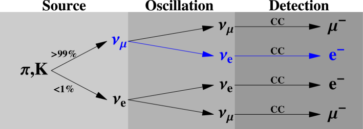
Figure 1: Schematic overview of neutrino production, oscillation and detection via charged current interactions for conventional beams and superbeams. The interesting channels are the ${\nu_{\mu}\rightarrow\nu_{\mu}}$ and ${\nu_{\mu}\rightarrow\nu_{e}}$ disappearance and appearance channels. The $\nu_{e}$ beam contamination at the level of $<1\%$ limits the ability to determine the ${\nu_{\mu}\rightarrow\nu_{e}}$ appearance oscillation, since it produces also electrons without oscillation. The $\nu_{\tau}$ oscillation channel is not shown here, but it would become very important if tau lepton detection is feasible. This requires energies sufficient for tau production and detectors with suitable tau lepton detection capabilities.

The neutrino beam is, however, contaminated by approximately $0.5\%$ electron neutrinos, which also produce electron reactions in the disappearance channel, limiting thus the precision in the extraction of ${\nu_{\mu}\rightarrow\nu_{e}}$ oscillation parameters. The energy spectrum of the muon beam can be controlled over a wide range: it depends on the incident proton energy, the optical system, and the precise direction of the beam axis compared to the direction of the detector. It is possible to produce broad band high energy beams, such as the CNGS beam [25, 26], or narrow band lower energy beams, such as in some configurations of the NuMI beam [27]. Reversing the electrical current in the lens system results in an anti-neutrino beam. The neutrino and anti-neutrino beams have significant differences such that errors do not cancel systematically in ratios or differences. The neutrino and anti-neutrino beams must therefore more or less be considered as independent sources with different systematical errors.

So-called “superbeams” are based on the same beam dump techniques for producing neutrino beams, but at much larger luminosities [25, 26, 27, 28]. Superbeams are thus a technological extrapolation of conventional beams, but use a proton beam intensity close to the mechanical stability limit of the target at a typical thermal power of $0.7\,\mathrm{MW}$ to $4\,\mathrm{MW}$. The much higher neutrino luminosity allows the use of the decay kinematics of pions to produce so–called “off–axis beams”, where the detector is located some degrees off the main beam axis. This reduces the neutrino flux and the average neutrino energy, but leads to a more mono-energetic beam and a significant suppression of the electron neutrino contamination. Several off–axis superbeams with energies of about $1\,\mathrm{GeV}$ to $2\,\mathrm{GeV}$ have been proposed in Japan [29, 30], America [31], and Europe [32, 33].

The most sensitive neutrino oscillation channel for sub-leading oscillation parameters is the ${\nu_{\mu}\rightarrow\nu_{e}}$ appearance transition. Therefore the detector should have excellent electron and muon charged current identification capabilities. In addition, an efficient rejection of neutral current events is required, because the neutral current interaction mode is flavor blind. With low statistics, the magnitude of the contamination itself limits the sensitivity to the ${\nu_{\mu}\rightarrow\nu_{e}}$ transition severely, while the insufficient knowledge of its magnitude constrains the sensitivity for high statistics. A near detector allows a substantial reduction of the background uncertainties [29, 34] and plays a crucial role in controlling other systematical errors, such as the flux normalization, the spectral shape of the beam, and the neutrino cross section at low energies. At energies of about $1\,\mathrm{GeV}$, the dominant charge current interaction mode is quasi–elastic scattering, which suggests that water Cherenkov detectors are the optimal type of detector. At these energies, a baseline of about $300\,\mathrm{km}$ would be optimal to measure at the first maximum of the oscillation. At about $2\,\mathrm{GeV}$, there is already a considerable contribution of inelastic scattering to the charged current interactions, which means that it would be useful to measure the energy of the hadronic part of the cross section. This favors low–Z hadron calorimeters, which also have a factor of ten better neutral current rejection capability compared to water Cherenkov detectors [31]. In this case, the optimum baseline is around $600\,\mathrm{km}$. The matter effects are expected to be small for these experiments for two reasons. First of all, an energy of about $1\,\mathrm{GeV}$ to $2\,\mathrm{GeV}$ is small compared to the MSW resonance energy of approximately $13\,\mathrm{GeV}$ in the upper mantle of the Earth. The second reason is that the baseline is too short to produce significant matter effects.

The second type of beam considered are so-called neutrino factories, where muons are stored in the long straight sections of a storage ring. The decaying muons produce muon and electron anti-neutrinos in equal numbers [35]. The muons are produced by pion decays, where the pions are produced by the same technique as for superbeams. After being collected, they have to be cooled and reaccelerated very quickly. This has not yet been demonstrated and it is the major technological challenge for neutrino factories [36]. The spectrum and flavor content of the beam are completely characterized by the muon decay and are therefore very precisely known [37]. The only adjustable parameter is the muon energy $E_{\mu}$, which is usually considered in the range from $20$ to $50\,\mathrm{GeV}$. In a neutrino factory it is also possible to produce and store anti-muons in order to obtain a CP conjugated beam. The symmetric operation of both beams leads to the cancellation or significant reduction of errors and systematical uncertainties. We will discuss in the following the neutrino beam, which implies always implicitly – unless otherwise stated – the CP conjugate channel.

The decay of the muons and the relevant oscillation channels are shown in fig. 2.

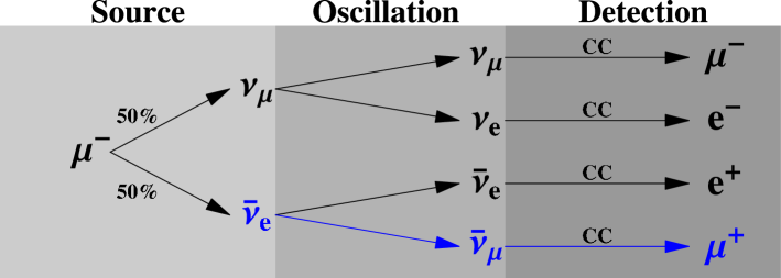
Figure 2: Neutrino production, oscillation and detection via charged current interactions for a neutrino factory for one polarity. $\overline{\nu}_{e}$ and $\nu_{\mu}$ are produced in equal numbers from $\mu$-decays and can undergo different oscillations. The ${\nu_{\mu}\rightarrow\nu_{\mu}}$ and ${\overline{\nu}_{e}\rightarrow\overline{\nu}_{\mu}}$ channels are most interesting for detectors with $\mu$ identification. Note, however, that excellent charge identification capabilities are required to separate “wrong sign muons” and “right sign muons”. The $\nu_{\tau}$ oscillation channel is not shown here, but it would become important if detectors with tau identification capabilities can be built.

Amongst all flavors and interaction types, muon charged current events are the easiest to detect. The appearance channel with the best sensitivity is thus the ${\overline{\nu}_{e}\rightarrow\overline{\nu}_{\mu}}$ transition, which produces so called “wrong sign muons”. Therefore, a detector must be able to very reliably identify the charge of a muon in order to distinguish wrong sign muons in the appearance channel from the higher rate of same sign muons in the disappearance channels. The dominant charge current interaction in the multi–GeV range is deep–inelastic scattering, making a good energy resolution for the hadronic energy deposition necessary. Magnetized iron calorimeters are thus the favored choice for neutrino factory detectors. In order to achieve the required muon charge separation, it is necessary to impose a minimum muon energy cut at approximately $4\,\mathrm{GeV}$ [38, 39]. This leads to a significant loss of neutrino events in the range of about $4\,\mathrm{GeV}$ to $20\,\mathrm{GeV}$, which means that a high muon energy of $E_{\mu}=50\,\mathrm{GeV}$ is desirable. The first oscillation maximum lies then at approximately $3\,000\,\mathrm{km}$. Matter effects are sizable at this baseline and energy and the limited knowledge of the Earth’s matter density profile becomes an additional source of errors.

Finally so-called $\beta$-beams are an interesting type of beam. The idea is to store radioactive isotopes in a storage ring similar to the muons in the neutrino factory, such that the $\beta$-decays of the radioactive elements lead to pure $\nu_{e}$ or $\overline{\nu}_{e}$ beams with $\gamma\simeq 100$ [40]. The energy spectrum of the neutrinos in the beam is determined by the neutrino energies of the decay at rest, boosted by the $\gamma$ factor, resulting typically in beam energies of a few hundred MeV at acceleration energies of about $100$ GeV per nucleon. There are technological and environmental challenges and it is unclear if $\beta$-beams can become an affordable and competitive neutrino source. We will not include $\beta$ beams in our quantitative discussion, but we will see that superbeams and neutrino factories have already an impressive potential, which could only be improved if $\beta$-beams were realized.

3 The Oscillation Framework

Most existing results on neutrino oscillations can so far be understood in an effective two neutrino framework with the well known oscillation probability for a baseline $L$ and neutrino energy $E_{\nu}$

$$P(\nu_{f_{1}}\rightarrow\nu_{f_{2}})=\left|\left\langle\nu_{f_{1}}(t)|\nu_{f_{2}}(t=0)\right\rangle\right|^{2}=\sin^{2}2\theta\cdot\sin^{2}\left(\frac{\Delta m^{2}L}{4E_{\nu}}\right)~{},$$ (1)

where $\theta$ is the mixing angle between the two flavour eigenstates $f_{1}$ and $f_{2}$ and where ${\Delta m^{2}}=m_{2}^{2}-m_{1}^{2}$ is the difference between the mass eigenvalues. Precision measurements at future LBL experiments involve a very precise knowledge of the sources, the detectors and the oscillation framework in matter. An effective two neutrino description is therefore definitively not adequate and matter effects must be included into the three neutrino oscillation framework.

The generalization of the oscillation formulae in vacuum to the case of $N$ neutrinos leads to the probabilities for flavour transitions $\nu_{f_{l}}\rightarrow\nu_{f_{m}}$ given by

$$P(\nu_{f_{l}}\rightarrow\nu_{f_{m}})=\underbrace{\delta_{lm}-4\sum_{i>j}\mathrm{Re}J_{ij}^{f_{l}f_{m}}\sin^{2}\Delta_{ij}}_{{\mathbf{\begin{picture}(20.0,7.0)\put(0.0,0.0){$P_{CP}$} \end{picture}}}}~{}\underbrace{-2\sum_{i>j}\mathrm{Im}J_{ij}^{f_{l}f_{m}}\sin 2\Delta_{ij}}_{{\mathbf{\begin{picture}(20.0,7.0)\put(5.0,-2.0){\line(2,1){14.0}} \put(0.0,0.0){$P_{CP}$} \end{picture}}}}$$ (2)

where the shorthands $J_{ij}^{f_{l}f_{m}}:=U_{li}U_{lj}^{*}U^{*}_{mi}U_{mj}$ and $\Delta_{ij}:=\frac{\Delta m^{2}_{ij}L}{4E}$ have been used. These generalized vacuum transition probabilities depend on all combinations of quadratic mass differences $\Delta m^{2}_{ij}=m_{i}^{2}-m_{j}^{2}$ as well as on different products of elements of the leptonic mixing matrix $U$.

We will assume for the rest of this article a three neutrino framework which can easily be generalized to more neutrinos if necessary. We have thus $1\leq i,j\leq 3$ and $U$ simplifies to the $3\times 3$ mixing matrix

$$U=\left(\begin{array}[]{ccc}c_{12}c_{13}&s_{12}c_{13}&s_{13}e^{-i\delta}\\ -s_{12}c_{23}-c_{12}s_{23}s_{13}e^{i\delta}&c_{12}c_{23}-s_{12}s_{23}s_{13}e^{i\delta}&s_{23}c_{13}\\ s_{12}s_{23}-c_{12}c_{23}s_{13}e^{i\delta}&-c_{12}s_{23}-s_{12}c_{23}s_{13}e^{i\delta}&c_{23}c_{13}\\ \end{array}\right)~{},$$ (3)

which contains three leptonic mixing angles and one Dirac-like leptonic CP phase $\delta$. Note that the most general mixing matrix for three Majorana neutrinos contains two further Majorana-like CP phases. However, it can easily be seen that these two extra diagonal Majorana phases do not enter in the above oscillation formulae and therefore we can omit them safely. Three neutrino oscillations depend thus in general only on the three mixing angles and one CP-phase. Disappearance probabilities, i.e. the transitions $\nu_{f_{l}}\rightarrow\nu_{f_{l}}$, do not even depend on this CP-phase, since $J_{ij}^{f_{l}f_{l}}$ is only a function of the modulus of elements of $U$. Appearance probabilities, like $\nu_{e}\rightarrow\nu_{\mu}$ are therefore the place where leptonic CP violation can be studied.

From eq. (2) the oscillation probabilities for neutrinos are $P(\nu_{f_{l}}\rightarrow\nu_{f_{m}})=\begin{picture}(20.0,7.0)\put(0.0,0.0){$P_{CP}$} \end{picture}+\begin{picture}(20.0,7.0)\put(5.0,-2.0){\line(2,1){14.0}} \put(0.0,0.0){$P_{CP}$} \end{picture}$ and for anti-neutrinos $P(\overline{\nu}_{f_{l}}\rightarrow\overline{\nu}_{f_{m}})=\begin{picture}(20.0,7.0)\put(0.0,0.0){$P_{CP}$} \end{picture}-\begin{picture}(20.0,7.0)\put(5.0,-2.0){\line(2,1){14.0}} \put(0.0,0.0){$P_{CP}$} \end{picture}$. Eq. (2) has thus a CP conserving part , and a CP violating part , and both terms depend on the CP phase $\delta$. An extraction strategy for CP-violation seems thus given by looking at the CP asymmetries [41]

$${a^{CP}:=\frac{P(\nu_{f_{l}}\rightarrow\nu_{f_{m}})-P(\overline{\nu}_{f_{l}}\rightarrow\overline{\nu}_{f_{m}})}{P(\nu_{f_{l}}\rightarrow\nu_{f_{m}})+P(\overline{\nu}_{f_{l}}\rightarrow\overline{\nu}_{f_{m}})}=\frac{{}^{\begin{picture}(20.0,7.0)\put(5.0,-2.0){\line(2,1){14.0}} \put(0.0,0.0){$P_{CP}$} \end{picture}}}{{}_{\begin{picture}(20.0,7.0)\put(0.0,0.0){$P_{CP}$} \end{picture}}}}~{}.$$ (4)

Note, however, that the beams of a LBL experiment traverse the Earth on a certain path and the presence of matter violates by itself CP, which modifies eq. (2) and which makes a measurement of leptonic CP violation more involved. The above general oscillation formulae in vacuum, eq. (2), lead to well known, but rather lengthy trigonometric expressions for the oscillation probabilities in vacuum. These expressions become even longer and do not exist in closed form when arbitrary matter corrections are taken into account. However, the problem simplifies somewhat under the assumption of a spherically symmetric Earth matter distribution [42] as shown in fig. 3 as function of the Earth radius.

Figure 3: The matter density profile of the Earth as a function of the radius $r$ [42]. Such matter density profiles are obtained by combining different data coming from geology, material science, seismology and astronomy under the assumption of spherically symmetry.

There is a one to one correspondence between the baseline $L$ and the angle under which the beam must enter the Earth at the source. Some examples are given in table 1 and obviously large $L$ corresponds to steep angles, resulting in technological and environmental challenges.

baseline $L$ in km	2800	7300	12750
angle in degrees	13	35	90

Table 1: Examples for oscillation lengths $L$ of long baseline experiments and the corresponding angle under which the beam enters and leaves the Earth near the source and near the detector.

Matter effects depend then in a first approximation only on the average matter density along the path between source and detector where fluctuations in the density profiles partially average out, but density errors must nevertheless be taken into account [43]. Matter effects in the oscillation formulae generally grow with distance $L$, while average density profile uncertainties tend to decrease with $L$, leading approximately to a constant error which we assume to be about $5\%$. Non-constant matter profiles can in principle lead to very interesting oscillation effects [44, 45, 46, 47, 48, 49]. Observing such effects would be very interesting, but they do not affect the studied experiments and they would just complicate the analysis of the oscillation parameter space. Fig. 3 shows at $r/R_{E}\simeq 0.5$ the pronounced density jump between the Earth mantle and the iron core and the average density approximation becomes much worse for beams which pass the core. Avoiding the iron core and the associated density jump corresponds to baselines of $L\leq{\cal O}(10\hskip 5.69054pt000~{}\mathrm{km})$. Matter effects lead to an MSW resonance at a characteristic energy. It is interesting to note that this resonance energy lies for the atmospheric ${\Delta m^{2}_{31}}$ and the given Earth matter density of about $3.8\mathrm{g/cm}^{3}$ in the crust at $E_{\mathrm{r}esonance}\simeq 10-15~{}$GeV.

The addition of arbitrary matter effects would make the oscillation formulae in general rather complicated, but the problem becomes much simpler for the case of three neutrinos and approximately constant average matter density. The Hamiltonian describing three neutrino oscillation in matter can be written in flavour basis as

$$H=\frac{1}{2E_{\nu}}U\left(\begin{array}[]{ccc}m_{1}^{2}&0&0\\ 0&m_{2}^{2}&0\\ 0&0&m_{3}^{2}\end{array}\right)U^{T}+\frac{1}{2E_{\nu}}\left(\begin{array}[]{ccc}A+A^{\prime}&0&0\\ ~{}0{}&~{}A^{\prime}{}&~{}0{}\\ ~{}0{}&~{}0{}&~{}A^{\prime}{}\end{array}\right)~{}.$$ (5)

The first term describes oscillations in vacuum in flavour basis. The quantities $A$ and $A^{\prime}$ in the second term are given by the charged current and neutral current contributions to coherent forward scattering in matter. The charged current contribution is given by

$$A=\pm~{}\frac{2\sqrt{2}G_{F}Y\rho E_{\nu}}{m_{n}}~{},$$ (6)

where $G_{F}$ is Fermi’s constant, $Y$ is the number of electrons per nucleon, $m_{n}$ is the nucleon mass and $\rho$ is the matter density. A is positive for neutrinos in matter and anti-neutrinos in anti-matter, while it is negative for anti-neutrinos in matter and neutrinos in anti-matter. The flavour universal neutral current contributions $A^{\prime}$ lead to an overall phase which does not enter the transition probabilities. The over-all neutrino mass scale $m_{1}^{2}$ can be written as a term proportional to the unit matrix and can similarly be removed, such that only ${\Delta m^{2}_{21}}$ and ${\Delta m^{2}_{31}}$ remain in the first term of eq. (5). Since ${\Delta m^{2}_{21}}\ll{\Delta m^{2}_{31}}$ we may further approximately set ${\Delta m^{2}_{21}}\simeq 0$ and we obtain thus the approximately equivalent Hamiltonian

$$H^{\prime}=\frac{1}{2E_{\nu}}U\left(\begin{array}[]{ccc}~{}0{}&~{}0{}&0\\ ~{}0{}&~{}0{}&0\\ ~{}0{}&~{}0{}&{\Delta m^{2}_{31}}\end{array}\right)U^{T}+\frac{1}{2E_{\nu}}\left(\begin{array}[]{ccc}A&0&0\\ 0&0&0\\ 0&0&0\end{array}\right)~{}.$$ (7)

The mixing matrix $U$ can furthermore be written as a sequence of rotations $R_{ij}$ in the two dimensional sub-spaces $ij$, namely

$$U=R_{23}\cdot R_{13}\cdot R_{12}~{},$$ (8)

where the 12 and 23 rotations are real, i.e. $R^{T}_{12}=R^{-1}_{12}$ and $R^{T}_{23}=R^{-1}_{23}$. This can be used to simplify the problem further, since $R_{12}$ commutes obviously with $diag(0,0,{\Delta m^{2}_{31}})$ and the $\theta_{12}$ dependence disappears from eq. (7). Next we observe that $diag(A,0,0)$ commutes with $R_{23}$, such that $R_{23}$ can be factored out from the complete Hamiltonian in eq. (7), which can therefore be re-written as

$$H^{\prime}=R_{23}\left[\frac{1}{2E_{\nu}}R_{13}\left(\begin{array}[]{ccc}~{}0{}&~{}0{}&0\\ ~{}0{}&~{}0{}&0\\ ~{}0{}&~{}0{}&{\Delta m^{2}_{31}}\end{array}\right)R_{13}^{T}+\frac{1}{2E_{\nu}}\left(\begin{array}[]{ccc}A&0&0\\ 0&0&0\\ 0&0&0\end{array}\right)\right]R_{23}^{T}~{}.$$ (9)

Inside the square bracket of eq. (9) the original mass matrix is rotated by $R_{13}$. The matter dependent part is then added inside the square bracket, while $R_{23}$ was factored out. $H^{\prime}$ is thus diagonalized by $R_{23}R^{\prime}_{13}$ and it becomes clear that we deal with a modification of the diagonalization of the 1-3 subspace. Matter effects lead therefore to an $A$-dependent parameter mapping in the 1-3 subspace which can be written as

$$\sin^{2}2\theta_{13,m} = \frac{\sin^{2}2\theta_{13}}{C_{\pm}^{2}}~{},$$ (10)

$${\Delta m^{2}_{31,m}} = {\Delta m^{2}_{31}}C_{\pm}~{},$$ (11)

$${\Delta m^{2}_{32,m}} = \frac{{\Delta m^{2}_{31}}~{}(C_{\pm}+1)+A}{2}~{},$$ (12)

$${\Delta m^{2}_{21,m}} = \frac{{\Delta m^{2}_{31}}~{}(C_{\pm}-1)-A}{2}~{},$$ (13)

where the index $m$ denotes effective quantities in matter and where

$$C^{2}_{\pm}=\left(\frac{A}{{\Delta m^{2}_{31}}}-\cos 2\theta\right)^{2}+\sin^{2}2\theta~{}.$$ (14)

Note that $A$ in $C_{\pm}$ can change its sign and the mappings for neutrinos and anti-neutrinos are therefore different, resulting in different effective mixings and masses. This is an important effect, which will allow detailed tests of coherent forward scattering of neutrinos in matter at future LBL experiments. Note that oscillations in matter depend unlike vacuum oscillations via $C_{\pm}$ on the sign of ${\Delta m^{2}_{31}}$. This is very interesting, since it opens the possibility to extract the $sign({\Delta m^{2}_{31}})$ via matter effects.

Another very interesting question is whether it will be possible to establish leptonic CP violation at future LBL experiments. Therefore we note that in the oscillation probabilities, eq. (2), all CP-violating effects are proportional to the following two quantities, namely

$$D = \sin\Delta_{21}\sin\Delta_{32}\sin\Delta_{31}~{},$$ (15)

$$8J_{\mathrm{CP}} = \cos\theta_{13}\sin(2\theta_{13})\sin(2\theta_{12})\sin(2\theta_{23})\sin\delta~{}.$$ (16)

We can immediately see from eq. (15) that CP violation is only possible if all three masses are different, i.e. if none of the ${\Delta m^{2}_{ij}}$ vanishes. For the considered LBL experiments we have $\Delta_{32}\simeq\Delta_{31}\simeq 1$ while $\sin\Delta_{21}\approx\Delta_{21}\ll 1$ and there is thus a suppression due to the small solar mass splitting. Furthermore we can see from eq. (16) that $J_{\mathrm{CP}}$ is suppressed by the small value of $\theta_{13}$ and for the small mixing angle solution in addition by $\theta_{12}$. The largest CP violating effects occur thus when $\theta_{12}$ is large and for the largest possible solar ${\Delta m^{2}_{21}}$, i.e. the LMA solution, which interestingly happens to be the solution which is clearly favoured by data.

Putting everything together leads still to quite lengthy expressions for the oscillation probabilities in matter, where it is not easy to oversee all effects. It is therefore instructive to simplify the problem to a point, where an analytic understanding of all effects is possible, while quantitative statements should be obtained with the help of numerical evaluations using the full expressions. The key for further simplification is to expand the oscillation probabilities in small quantities. These expansion parameters are $\alpha={\Delta m^{2}_{21}}/{\Delta m^{2}_{31}}\simeq 10^{-2}$ and $\sin^{2}2\theta_{13}\leq 0.1$. The matter effects can be parametrized by the dimensionless quantity $\hat{A}=A/{\Delta m^{2}_{31}}=2VE/{\Delta m^{2}_{31}}$, where $V=\sqrt{2}G_{F}n_{e}$. Using $\Delta\equiv\Delta_{31}$, the leading terms in this expansion are, for example, for $P(\nu_{\mu}\rightarrow\nu_{\mu})$ and $P(\nu_{e}\rightarrow\nu_{\mu})$ [50, 51, 52]

$$P(\nu_{\mu}\rightarrow\nu_{\mu})\approx$$

$$1-\cos^{2}\theta_{13}\sin^{2}2\theta_{23}\sin^{2}{\Delta}+2~{}{\alpha}~{}\cos^{2}\theta_{13}\cos^{2}\theta_{12}\sin^{2}2\theta_{23}{\Delta}\cos{\Delta},$$ (17)

$$P(\nu_{e}\rightarrow\nu_{\mu})\approx{\sin^{2}2\theta_{13}}\sin^{2}\theta_{23}~{}~{}\frac{\sin^{2}({(1\!\!-\!\hat{A})}{\Delta})}{{(1\!\!-\!\hat{A})^{2}}}$$

$$\pm~{}{\sin\delta}\cdot{\sin 2\theta_{13}}~{}{\alpha}~{}\sin 2\theta_{12}\cos\theta_{13}\sin 2\theta_{23}\sin({\Delta})\frac{\sin({\hat{A}}{\Delta})\sin({(1\!\!-\!\hat{A})}{\Delta})}{{\hat{A}(1\!\!-\!\hat{A})}}$$

$$+\cos\delta\cdot{\sin 2\theta_{13}}~{}{\alpha}~{}\sin 2\theta_{12}\cos\theta_{13}\sin 2\theta_{23}\cos({\Delta})\frac{\sin({\hat{A}}{\Delta})\sin({(1\!\!-\!\hat{A})}{\Delta})}{{\hat{A}(1\!\!-\!\hat{A})}}$$

$$+~{}{\alpha^{2}}~{}\sin^{2}2\theta_{12}\cos^{2}\theta_{23}\frac{\sin^{2}({\hat{A}}{\Delta})}{{\hat{A}^{2}}}~{},$$ (18)

where in eq. (18) “$+$” stands for neutrinos and “$-$” for anti-neutrinos. The most important feature of eq. (18) is that all interesting effects in the ${\nu_{e}\rightarrow\nu_{\mu}}$ transition depend crucially on $\theta_{13}$. The size of $\sin^{2}2\theta_{13}$ determines thus if the total transition rate, matter effects, effects due to the sign of ${\Delta m^{2}_{31}}$ and CP violating effects are measurable. One of the most important questions for future LBL experiments is therefore how far experiments can push the $\theta_{13}$ limit below the current CHOOZ bound of approximately $\sin^{2}2\theta_{13}<0.1$.

Before we discuss further important features of eqs. (17) and (18) in more detail we would like to comment once more on the underlying assumptions and the reliability of these equations. First eqs. (17) and (18) are an expansion in terms of the small quantities $\alpha$ and $\sin 2\theta_{13}$. Higher order terms are suppressed at least by another power of one of these small parameters and these corrections are thus typically at the percent level. The matter corrections in eqs. (17) and (18) are derived for constant average matter density. Numerical test have shown that this approximation works quite well as long as the matter profile is reasonably smooth. A number of very interesting effects existing in general non-constant matter distributions are therefore only small theoretical uncertainties. An example is given by asymmetric matter profiles, which lead to interesting T-violating effects [53], but this does not play a role here since the Earth is sufficiently symmetric.

Note that all results which will be shown later are based on numerical simulations of the full problem in matter. These results do therefore not depend on any approximation. Eqs. (17) and (18) will only be used to understand the problem analytically, which is extremely helpful in order to oversee the six (or more) dimensional parameter space. The full numerical analysis and eqs. (17) and (18) depend, however, on the assumption of a standard three neutrino scenario. It is thus assumed that the LSND signal [54] will not be confirmed by the MiniBooNE experiment [55]. Neutrinos could in principle decay, which would make the analysis much more involved. It is assumed in this article that neutrinos are stable, and a combined treatment of oscillation and decay [56] would be much more involved. Neutrinos might further have unusual properties and might, for example, violate CPT. In that case neutrinos and anti-neutrinos could have different properties and LBL experiments can give very interesting limits on this possibility [57], but we will assume in this study that CPT is preserved.

4 Correlations and Degeneracies

Eqs. (17) and (18) exhibit certain parameter correlations and degeneracies, which play an important role in the analysis of LBL experiments, and which would be hard to understand in a purely numerical analysis of the high dimensional parameter space. The most important properties are:

• First we observe that eqs. (17) and (18) depend only on the product $\alpha\cdot\sin 2\theta_{12}$ or equivalently ${\Delta m^{2}_{21}}\cdot\sin 2\theta_{12}$. This are the parameters related to solar oscillations which will be taken as external input. The fact that only the product enters, implies that it may be better determined than the product of the measurements of ${\Delta m^{2}_{21}}$ and $\sin 2\theta_{12}$.

• Next we observe in eq. (18) that the second and third term contain both a factor $\sin(\hat{A}\Delta)$, while the last term contains a factor $\sin^{2}(\hat{A}\Delta)$. Since $\hat{A}\Delta=2VL$, we find that these factors depend only on $L$, resulting in a “magic baseline” when $2VL_{magic}=\pi/4V$, where $\sin(\hat{A}\Delta)$ vanishes. At this magic baseline only the first term in eq. (18) survives and $P(\nu_{e}\rightarrow\nu_{\mu})$ does no longer depend on $\delta$, $\alpha$ and $\sin 2\theta_{12}$. This is in principle very important, since it implies that $\sin^{2}2\theta_{13}$ can be determined at the magic baseline from the first term of eq. (18) whatever the values and errors of $\delta$, $\alpha$ and $\sin 2\theta_{12}$ are. For the matter density of the Earth we find

  $$L_{magic}=\pi/4V\simeq 8100~{}\mathrm{\rm km}~{},$$ (19)

  which is an amazing number, since the value of $V$ could be such that $L_{magic}$ is very different from the scales under discussion.

• Next we observe that only the second and third term of eq. (18) depend on the CP phase $\delta$, and both terms contain a factor $\sin 2\theta_{13}\cdot\alpha$, while the first and fourth term of eq. (18) do not depend on the CP phase $\delta$ and contain factors of $\sin^{2}2\theta_{13}$ and $\alpha^{2}$, respectively. The extraction of CP violation is thus always suppressed by the product $\sin 2\theta_{13}\cdot\alpha$ and the CP violating terms are furthermore obscured by large CP independent terms if either $\sin^{2}2\theta_{13}\ll\alpha^{2}$ or $\sin^{2}2\theta_{13}\gg\alpha^{2}$. The determination of the CP phase $\delta$ is thus best possible if $\sin^{2}2\theta_{13}\simeq 4\theta^{2}_{13}\simeq\alpha^{2}$.

• Another observation is that the last term in eq. (18), which is proportional to $\alpha^{2}=({\Delta m^{2}_{21}})^{2}/({\Delta m^{2}_{31}})^{2}$, dominates in the limit of tiny $\sin^{2}2\theta_{13}$. The error of ${\Delta m^{2}_{21}}$ limits therefore for small $\sin^{2}2\theta_{13}$ the parameter extraction.

• Eqs. (17) and (18) have a structure which suggests that transformations exist, which leave these equations invariant. We expect therefore degeneracies, i.e. for given $L/E$ parameter sets with identical oscillation probabilities. An example of such an invariance is given by a simultaneous replacement of neutrinos by anti-neutrinos and ${\Delta m^{2}_{31}}\rightarrow-{\Delta m^{2}_{31}}$. This is equivalent to changing the sign of the second term of eq. (18) and replacing $\alpha\rightarrow-\alpha$ and $\Delta\rightarrow-\Delta$, while $\hat{A}\rightarrow\hat{A}$. It is easy to see that eqs. (17) and (18) are unchanged, but this constitutes no degeneracy, since we can distinguish neutrinos and anti-neutrinos experimentally.

• The first real degeneracy [58] can be seen in the disappearance probability eq. (17), which is invariant under the replacement $\theta_{23}\rightarrow\pi/2-\theta_{23}$. Note that the second and third term in eq. (18) are not invariant under this transformation, but this change in the sub-leading appearance probability can approximately be compensated by small parameter shifts. However, the degeneracy can in principle be lifted with precision measurements in the disappearance channels.

• The second degeneracy can be found in the appearance probability eq. (18) in the ($\delta-\theta_{13}$)-plane [59]. In terms of $\theta_{13}$ (which is small) and $\delta$ the four terms of eq. (18) have the structure

  $$P(\nu_{e}\rightarrow\nu_{\mu})\approx\theta^{2}_{13}\cdot F_{1}+\theta_{13}\cdot(\pm~{}\sin\delta F_{2}+\cos\delta F_{3})+F_{4}~{},$$ (20)

  where the quantities $F_{i}$, $i=1,..,4$ contain all the other parameters. The requirement $P(\nu_{e}\rightarrow\nu_{\mu})=const.$ leads for both neutrinos and anti-neutrinos to parameter manifolds of degenerate or correlated solutions. Having both neutrino and anti-neutrino beams, the two channels can be used independently, which is equivalent to considering simultaneously eq. (20) for $F_{2}\equiv 0$ and $F_{3}\equiv 0$. The requirement that these probabilities are now independently constant, i.e. $P(\nu_{e}\rightarrow\nu_{\mu})=const.$ for $F_{2}\equiv 0$ and $F_{3}\equiv 0$, leads to more constraint manifolds in the ($\delta-\theta_{13}$)-plane, but some degeneracies still survive.

• The third degeneracy [60] is given by the fact that a change in sign of ${\Delta m^{2}_{31}}$ can essentially be compensated by an offset in $\delta$. Therefore we note again that the transformation ${\Delta m^{2}_{31}}\rightarrow-{\Delta m^{2}_{31}}$ leads to $\alpha\rightarrow-\alpha$, $\Delta\rightarrow-\Delta$ and $\hat{A}\rightarrow-\hat{A}$. All terms of the disappearance probability, eq. (17), are invariant under this transformation. The first and fourth term in the appearance probability eq. (17), which do not depend on the CP phase $\delta$, are also invariant. The second and third term of eq. (17) depend on the CP phase and change by the transformation ${\Delta m^{2}_{31}}\rightarrow-{\Delta m^{2}_{31}}$. The fact that these changes can be compensated by an offset in the CP phase $\delta$ is the third degeneracy.

• Altogether there exists thus an eight-fold degeneracy [58], as long as only the ${\nu_{\mu}\rightarrow\nu_{\mu}}$, ${\overline{\nu}_{\mu}\rightarrow\overline{\nu}_{\mu}}$, ${\nu_{e}\rightarrow\nu_{\mu}}$ and ${\overline{\nu}_{e}\rightarrow\overline{\nu}_{\mu}}$ channels and one fixed $L/E$ are considered. However, the structure of eqs. (17) and (18) makes clear that the degeneracies can be broken by using in a suitable way information from different $L/E$ values. This can be achieved in total event rates by changing $L$ or $E$ [61, 62], but it can in principle also be done by using information in the event rate spectrum of a single baseline $L$, which requires detectors with very good energy resolution [52]. Another strategy to break the degeneracies is to include further oscillation channels in the analysis (“silver channels”) [63, 61].

The discussion of this section shows the strength of the analytic approximations, which allow to understand the complicated parameter interdependence. It also helps to optimally plan experimental setups and to find strategies to resolve the degeneracies.

5 Event Rates

The experimentally detected event rates must be compared with the theoretical expressions, which depend only indirectly on the above oscillation probabilities. Every event can be classified by the information on the flavor of the detected neutrino and the type of interaction. The particles detected in an experiment are produced by neutral current (NC), inelastic charged current (CC) or quasi–elastic charged current (QE) interactions. The contribution to each mode depends on a number of factors, like detector type, the neutrino energy and flavour. In order to calculate realistic event rates we compute first for each neutrino flavor and energy bin the number of events for each type of interaction in the fiducial mass of an ideal detector. Next the deficiencies of a real detector are included, like limited event reconstruction capabilities. The combined description leads to the differential event rate spectrum for each flavor and interaction mode as it would be seen by a detector which is able to separate all these channels. Finally different channels must be combined, since they can not be observed separately. This can be due to physics, e.g., due to the flavor–blindness of NC interactions, or it can be a consequence of detector properties, e.g., due to charge misidentification. The differential event rates can thus be written for each channel of the interaction type IT as

$$\frac{dn_{f}^{\mathrm{IT}}}{dE^{\prime}}= N\,\sum_{i}\int\int dE\,d\hat{E}\quad\underbrace{\Phi_{i}(E)}_{\mathrm{Production}}\times$$ (21)

$$\underbrace{\frac{1}{L^{2}}P_{(i\rightarrow f)}(E,L,\rho;\theta_{23},\theta_{12},\theta_{13},\Delta m^{2}_{31},\Delta m^{2}_{21},\delta)}_{\mathrm{Propagation}}~{}\times$$

$$\underbrace{\sigma^{\mathrm{IT}}_{f}(E)k_{f}^{\mathrm{IT}}(E-\hat{E})}_{\mathrm{Interaction}}~{}~{}\times~{}~{}\underbrace{T_{f}(\hat{E})V_{f}(\hat{E}-E^{\prime})}_{\mathrm{Detection}}~{},$$

where $f$ and $i$ stand for the final and initial neutrino flavor, respectively. $E$ is the incident neutrino energy, $\Phi_{i}(E)$ is the flux for the initial flavor $i$ from the source, $L$ is the baseline, $N$ is a normalization factor, and $\rho$ is the Earth matter density. The interaction term is composed of two factors, which are the total cross section $\sigma^{\mathrm{IT}}_{f}(E)$ for the flavor $f$ and the interaction type IT, and the energy distribution of the secondary particle $k_{f}^{\mathrm{IT}}(E-\hat{E})$, where $\hat{E}$ is the energy of the secondary particle. The detector threshold is parametrized by the function $T_{f}(\hat{E})$, describing limited resolution or cuts in the analysis. The energy resolution of the detector is parametrized by the function $V_{f}(\hat{E}-E^{\prime})$ for the secondary particle, where $E^{\prime}$ is the reconstructed neutrino energy.

The numerical calculation of the double integral of eq. (21) for all possible parameter combinations requires enormous computing power. We use therefore an approximation where we evaluate the integral over $\hat{E}$, where the only terms containing $\hat{E}$ are $k_{f}^{\mathrm{IT}}(E-\hat{E})$, $T_{f}(\hat{E})$, and $V_{f}(\hat{E}-E^{\prime})$. We define

$$R_{f}^{\mathrm{IT}}(E,E^{\prime})\,\epsilon_{f}^{\mathrm{IT}}(E^{\prime})\equiv\int d\hat{E}\quad T_{f}(\hat{E})\,k_{f}^{\mathrm{IT}}(E-\hat{E})\,V_{f}(\hat{E}-E^{\prime})~{},$$ (22)

and approximate $R_{f}^{\mathrm{IT}}$ by the analytical expression

$$R_{f}^{\mathrm{IT}}(E,E^{\prime})=\frac{1}{\sigma\sqrt{2\pi}}\exp{\frac{(E-E^{\prime})^{2}}{2\sigma^{2}}}~{}.$$ (23)

For QE interactions in JHF beam we will use [29] $\sigma=85$ MeV and for the neutrino factory and NuMI beams we use [64, 65] $\sigma=0.15\cdot E$. The values for the effective relative energy resolution $\delta E$ and the effective efficiency $\epsilon_{f}^{\mathrm{IT}}$ can be found in the literature, i.e. for the neutrino factory in [38, 39, 50, 66, 67] and for the superbeam setups in [29, 68, 69, 70, 71]. The threshold for muon detection is for neutrino factories an important parameter and we use essentially an interpolation between a more optimistic and a conservative attitude [39, 50]. For further details see [13].

In order to include backgrounds, the channels are grouped in an experiment specific way into pairs of signal and background. The considered backgrounds are NC–events which are misidentified as CC–events and CC–events identified with the wrong flavor or charge. For superbeams we include furthermore the background of CC–events coming from an intrinsic contamination of the beam.

Finally we combine in the analysis all available signal channels and perform a global fit to extract the physics parameters in an optimal way. The relevant channels are for a neutrino factory for each polarity of the beam the $\nu_{\mu}$–CC channel (disappearance) and $\overline{\nu}_{\mu}$–CC channel (appearance) event rate spectra. The backgrounds for these signals are NC events for all flavours and misidentified $\nu_{\mu}$–CC events. For superbeam experiments the signal is for each polarity of the beam given by the $\nu_{\mu}$–QE channel (disappearance) and ${\nu}_{e}$–CC channel (appearance). The backgrounds are here NC events for all flavors, misidentified $\nu_{\mu}$–CC events, and, for the ${\nu}_{e}$–CC channel, the $\nu_{e}$–CC beam contamination.

6 The Considered LBL Setups

The discussed sources and detectors allow different LBL experiments and it is interesting to compare their physics potential on an equal and as realistic as possible footing. Studies at the level of probabilities are not sufficient and the true potential must be evaluated at the level of event rates as described in section 5, with realistic assumptions about the beams, detectors and backgrounds. We present now the results of such an analysis which is essentially based on reference [13], where we calculate the oscillation probabilities with the exact three neutrino oscillation formulae in matter numerically, i.e. we use the approximations for the probabilities in eqs. (17) and (18) only for a qualitative understanding. All results shown below are therefore not affected by approximations which were made in the derivation of the approximate analytic oscillation formulae eqs. (17) and (18). Sensitivities etc. are defined by the ability to re-extract the physics parameters from a simulation of event rates. Therefore event rate distributions are generated for any possible parameter set. Subsequently a combined fit to these event rate distributions is performed simultaneously for the appearance and disappearance channels for both polarities. This procedure uses all the available information in an optimal way. It includes spectral distributions when present, and it reduces to a fit of total rates when the total event rates are small. Adequate statistical methods as described in [13] are used in order to deal with event distributions which have in some regions small event rates per bin. Systematical uncertainties are parametrized and external input from geophysics is used in form of the detailed matter profile and its errors, which are included in the analysis [13]. The ability to re-extract in a simulation of the full experiment the input parameters which were used to generate event rate distributions is used define sensitivities and precision.

An important aspect of such an analysis is the inclusion of external information. The discussed LBL experiments could in principle measure the solar ${\Delta m^{2}_{21}}$ and mixing angle $\theta_{12}$. However, the precision which can be obtained can not compete with the expected measurement of KamLand [72]. We include therefore as external input the assumption that KamLand measures the solar parameters in the center of the LMA region with typical errors. Otherwise all unknown parameters (like the CP phase) will not be constrained and are therefore left free, with all parameter degeneracies and error correlations taken into account. All nuisance parameters are integrated out and a projection on the parameter of interest is performed. Altogether we are dealing with six free parameters.

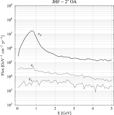
Figure 4: The flux of the $2^{o}$ off-axis JHF beam as a function of energy. The mean energy is $0.51\,\mathrm{GeV}$ and the peak intensity is $1.7\cdot 10^{7}\,\mathrm{GeV}^{-1}\,\mathrm{cm}^{-2}\,\mathrm{yr}^{-1}$ at $0.78\,\mathrm{GeV}$. The $\nu_{e}/\nu_{\mu}$-ratio is at the peak $0.2\%$.

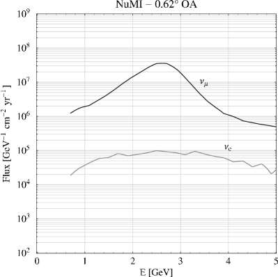
Figure 5: The flux of the proposed NuMI off-axis beam with a mean energy of $2.78\,\mathrm{GeV}$, a peak intensity of $3.6\cdot 10^{7}\,\mathrm{GeV}^{-1}\,\mathrm{cm}^{-2}\,\mathrm{yr}^{-1}$ at $2.18\,\mathrm{GeV}$. The $\nu_{e}/\nu_{\mu}$-ratio is at the peak $0.2\%$.

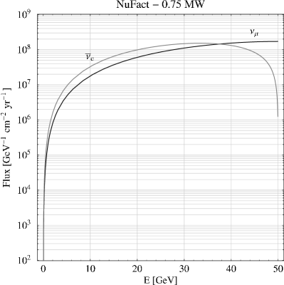
Figure 6: The flux of a neutrino factory with $E_{\mu}=50~{}\mathrm{GeV}$. The mean neutrino energy is about $30\,\mathrm{GeV}$, the peak intensity is $1.5\cdot 10^{8}\,\mathrm{GeV}^{-1}\,\mathrm{cm}^{-2}\,\mathrm{yr}^{-1}$ at $33.33\,\mathrm{GeV}$. The $\nu_{\mu}/\nu_{e}$-ratio is at the peak $83\%$.

The beam characteristics of the three considered sources are shown in figures 4 (JHF), 5 (NuMI off-axis) and 6 (neutrino factory). We also include uncertainties of these beam parameters, i.e. for the first two conventional beams uncertainties in the $\nu_{e}$–background and for all beams flux uncertainties [29, 31, 35]. As detectors we consider water Cherenkov detectors, low-Z calorimeters and magnetized iron detectors with parameters as given in table 2. For magnetized iron calorimeters it is important to include realistic threshold effects. We use a linear rise of the efficiency between $4\,\mathrm{GeV}$ and $20\,\mathrm{GeV}$ and we study the sensitivity to the threshold position. We do not include liquid Argon TPCs in our analysis, but they would certainly be an important detector if this technology will work.

	water Cherenkov	low-Z	magnetized iron
	= SK (HK)	calorimeter	calorimeter
fiducial mass	$22.5\,\mathrm{kt}$ ($1\,000\,\mathrm{kt}$)	$20\,\mathrm{kt}$	$10\,\mathrm{kt}$ ($50\,\mathrm{kt}$)
energy range	$0.4-1.2\,\mathrm{GeV}$	$1-5\,\mathrm{GeV}$	$4-50\,\mathrm{GeV}$
energy resolution	$85$ MeV	$0.15\cdot E$	$0.15\cdot E$
signal efficiency	$0.5$	$0.5$	$0.45$
NC rejection	$0.01$	$0.001$	$<10^{-5}$
CID	–	–	$<10^{-5}$
background uncertainty	$5\%$	$5\%$	$5\%$

Table 2: The considered detector types and their most important parameters.

The considered beams and detectors allow now different interesting combinations which are listed in table 3. JHF-SK is the planned combination of the existing SuperKamiokande detector and the JHF beam, while JHF-HK is the combination of an upgraded JHF beam with the proposed HyperKamiokande detector. With typical parameters, JHF-HK is altogether about $95$ times more integrated luminosity than JHF-SK, and we assume that it operates partly with the anti-neutrino beam. Water Cherenkov detectors are ideal for the JHF beam, since charged current quasi elastic scattering is dominating. NuMI is the proposed combination of the NuMI off-axis beam with a low-Z calorimeter, which is better here, since the energy is higher and there is already a considerable contribution of inelastic charged current interactions. NuFact-I is an initial neutrino factory, while NuFact-II is a fully developed machine, with $42$ times the luminosity of NuFact-I [29, 31, 38]. Deep inelastic scattering dominates for these even higher energies and magnetized iron detectors are therefore considered in combination with neutrino factories.

acronym	detector	baseline	matter density	$L/E_{\mathrm{peak}}$
JHF-SK	water Cherenkov	$295\,\mathrm{km}$	$2.8\,\mathrm{g}\,\mathrm{cm}^{-3}$	$378\,\mathrm{km}\,\mathrm{GeV}^{-1}$
NuMI	low-Z	$735\,\mathrm{km}$	$2.8\,\mathrm{g}\,\mathrm{cm}^{-3}$	$337\,\mathrm{km}\,\mathrm{GeV}^{-1}$
NuFact-I	$10$ kt magnetized iron	$3\,000\,\mathrm{km}$	$3.5\,\mathrm{g}\,\mathrm{cm}^{-3}$	$90\,\mathrm{km}\,\mathrm{GeV}^{-1}$
JHF-HK	water Cherenkov	$735\,\mathrm{km}$	$2.8\,\mathrm{g}\,\mathrm{cm}^{-3}$	$295\,\mathrm{km}\,\mathrm{GeV}^{-1}$
NuFact-II	$40$ kt magnetized iron	$3\,000\,\mathrm{km}$	$3.5\,\mathrm{g}\,\mathrm{cm}^{-3}$	$90\,\mathrm{km}\,\mathrm{GeV}^{-1}$

Table 3: The considered combinations of beams and detectors and their acronyms.

	JHF-SK	NuMI	JHF-HK	NuFact-I	NuFact-II
signal	$139.0$	$387.5$	$13\,180.0$	$1\,522.8$	$64\,932.6$
background	$23.3$	$53.3$	$2\,204.6$	$4.2$	$180.3$
S/N	$6$	$6$	$6$	$360$	$360$

Table 4: The expected signal and background event rates for the appearance channels for the considered scenarios.

7 The Qualitative Picture

A number of studies have analyzed various aspects of individual or some combined variants of the above scenarios [39, 50, 52, 58, 60, 73, 74, 75, 76, 77, 78, 79, 80, 81, 82, 83, 84, 85, 86, 87, 88, 89, 90, 13] and the results can all be understood by the same qualitative picture. The proposed setups lead in general to remarkably large event rates in the disappearance channel. This leads to many events per energy bin, and the spectral information allows very precise fits of the leading oscillation parameters ${\Delta m^{2}_{31}}$ and $\theta_{23}$. A typical example is shown for a neutrino factory in fig. 7 for both polarities [78].

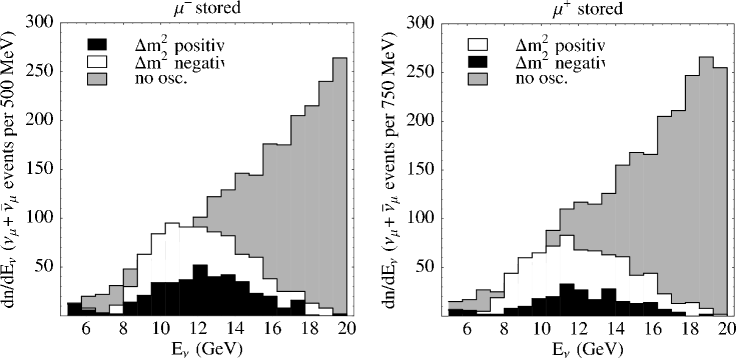
Figure 7: $\nu_{\mu}$ disappearance rates for a typical neutrino factory setup. The grey area marks the expected distribution in the absence of oscillations. The black and white histograms show the expected distributions with oscillations for both ${\Delta m^{2}_{31}}>0$ and ${\Delta m^{2}_{31}}<0$. Here a relatively large $\sin^{2}2\theta_{13}=0.01$ was chosen, where matter effects allow to extract $sign({\Delta m^{2}_{31}})$ even from the disappearance channel, which is not possible for smaller $\sin^{2}2\theta_{13}$ [78].

The situation is somewhat different in the appearance channels, where the event rates are small. The results depend thus for the appearance channels dominantly on total rates, with some spectral information. Note, however, that available spectral information is very important, since it allows to distinguish solutions which are degenerate on the basis of total event rates.

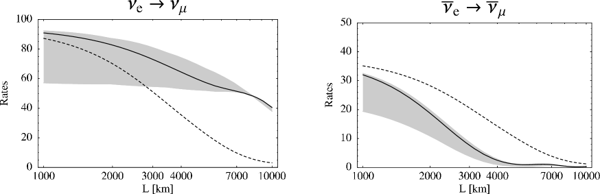
Figure 8: The total event rates for the two polarities of a neutrino factory with $E_{\mu}=50~{}$GeV and $\sin^{2}2\theta_{13}=0.01$ and the LMA solution. The solid lines are for $\delta=0$ with the matter corrections included. The dashed lines show for comparison $\delta=0$ in vacuum. The grey band shows the range where the solid line moves when the CP phase is allowed to take all possible values with matter included.

Fig. 8 shows how the total event rates depend for a neutrino factory with typical parameters on the presence of matter and on the CP phase. It can clearly be seen in fig. 8 that matter effects grow with distance and become dominating at large baselines of $L\mathrel{\vbox{\hbox{$>$}\nointerlineskip\hbox{$\sim$}}}3000~{}\mathrm{km}$. Contrary the CP phase $\delta$ affects the rates at shorter distances, while at medium distances comparable matter effects and CP violating effects are present. The simplest strategy to separate matter effects and CP violation is thus to have one short baseline for CP violating effects and another large baseline for matter effects [50, 62]. Alternatively one might use a single medium baseline, where the effects can be separated if the event rates are large enough such that spectral information can be extracted [52]. Another alternative is, as discussed before, to use one baseline and further oscillation channels [63].

It is interesting to understand the interplay of matter effects and CP violating effects from our analytic formulae. First we observe from eqs. (17) and (18) as well as fig. 8 that matter effects grow with distance and CP violating effects are thus not affected by matter effects at shortest distances. Inspecting carefully eq. (18) we found in section 4 for larger distances the existence of a magic baseline. The point was that $\hat{A}=2VE/{\Delta m^{2}_{31}}$ and $\Delta={\Delta m^{2}_{31}}L/E$, such that $\hat{A}\Delta=2VL$ depends only on the matter potential $V$ and the baseline $L$. All but the first term in eq. (18) vanish therefore for $L_{magic}$ as given in eq. (19), since they contain factors of $\sin(\hat{A}\Delta)=\sin(2VL)$. All terms which contain the CP phase $\delta$ and the mass splitting hierarchy parameter $\alpha$ vanish thus as a consequence of matter effects at $L_{magic}\simeq 8100~{}\mathrm{km}$, where a typical density in the Earth crust has been used. Matter effects and CP violating effects can thus in principle be completely separated by performing measurements at small baseline and at the magic baseline [91].

8 The Analysis

The sensitivity and the precision of the measured quantities are defined as explained in section 5 via the ability to re-extract the physics parameters from previously generated event rate distributions. In order to determine the sensitivity and the precision all input parameters are scanned while systematical, statistical and background errors are included. The best possible results are obtained by optimally using the information contained in the rates and in the energy spectrum of all available channels in a combined analysis. At the same time the parameter correlations and degeneracies mentioned above must be included in addition to systematical errors like normalization and calibration. However, precise relative information contained in the spectrum allows very precise measurements even for an included overall normalization error of $5\%$ and an energy calibration error of $5\%$. The inclusion of backgrounds limits the sensitivity. However, information in the energy spectrum helps to reduce the impact of the background, which has typically a different energy dependence.

There are many events per bin in the disappearance channels, which leads via eq. (17) to a very precise determination of the leading oscillation parameters ${\Delta m^{2}_{31}}$ and $\sin^{2}2\theta_{23}$. The combination of the available appearance channels allows to determine or restrict $\theta_{13}$, and via the matter effects $sign({\Delta m^{2}_{31}})$. This is always possible, even when $\alpha$ is tiny or negligible for the disfavoured SMA, LOW and VAC solutions of the solar neutrino problem, since the first term in eq. (18) does not depend on $\alpha$. For the LMA solution (i.e. $\alpha\simeq 10^{-2}$) it is possible to determine $\theta_{13}$, $sign({\Delta m^{2}_{31}})$, and it is in principle even possible to extract from a combined fit of the appearance and disappearance channels the solar parameters $\theta_{12}$ and ${\Delta m^{2}_{21}}$ without using external input. The precision which can be obtained for $\theta_{12}$ and ${\Delta m^{2}_{21}}$ can, however, not compete with the expected measurements of KamLand. We assume therefore in our analysis that KamLand measures the solar parameters at the current best fit of the LMA solution with typical errors and take this as external input for our analysis. This allows then for the favoured LMA solution to extract information on the CP phase $\delta$, as expected from the second and third term of eq. (18).

It should be kept in mind that eqs. (17) and (18) exhibit parameter correlations and degeneracies as discussed above, which must be taken into account in the analysis [50, 58, 59, 60, 52, 13]. The analytic formulae eqs. (17) and (18) are here extremely useful, since they allow to understand qualitatively the highly non-linear behaviour and the complex topology of the parameter manifolds. The parameter dependence in the probabilities leads, as discussed above, to three degeneracies in the following parameter planes:

• $\delta$-$\theta_{13}$

• $\delta$-$\mathrm{sign}({\Delta m^{2}_{31}})$

• $\theta_{23}$– ($\pi/2-\theta_{23}$)

These three different degeneracies can lead to equivalent solutions which can be rather close in parameter space. In this case they effectively enlarge the allowed range of the combined solutions as shown in an example for the $\delta-\theta_{13}$ plane in the left plot of fig. 9. In other cases the degenerate solutions are well separated, as it is shown, for example, in the right plot of fig. 9. In such cases it is more sensible to quote two values and their respective errors.

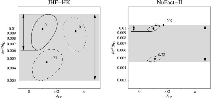
Figure 9: Examples of degenerate solutions [13]. The left plot shows a case where the degenerate solutions are very close. The combination of these adjacent solutions leads consequently to an enlarged error due to degeneracies. The right plot shows a case where two degenerate solutions are well separated. In this case two solutions and their respective errors should be quoted.

In a detailed single baseline analysis one can see, as discussed analytically in section 4, that the $\delta$-$\theta_{13}$ degeneracy becomes typically a parameter correlation as long as only a neutrino beam is used, while degenerate islands show up when both polarities are combined. Similarly one can see that with one baseline the $\delta$-$\mathrm{sign}({\Delta m^{2}_{31}})$ degeneracy can never be removed. The $\theta_{23}$–($\pi/2-\theta_{23}$) degeneracy can also not be removed as long as the analysis is dominated by the disappearance rates only. This degeneracy can be lifted for sufficiently high statistics in the appearance channel, where the degeneracy is in principle broken, as seen in the analytic discussion in section 4.

The separation of matter and CP violating effects is, as discussed in section 4, not possible at the level of total event rates for one value of $L/E$, which translates for fixed $E$ into one baseline. However, as mentioned before, there exist ways to break this degeneracy. One strategy was to use a short baseline for CP violating effects and a long baseline for matter effects. Another strategy was to use one single medium baseline and the information contained in the beam spectrum. The point is that different parameter sets were degenerate at the level of total event rates for one $L/E$, while the event rate distributions differ significantly. The degeneracy may thus be lifted for one medium baseline in combination with good resolution and sufficient statistics. This is shown in fig. 10 for the correlation of $\delta$ with $\theta_{13}$ [52].

Figure 10: The correlation or degeneracy of $\delta$ with $\theta_{13}$ as a function of the detector energy resolution for a neutrino factory with $E=50\,\mathrm{GeV}$, $L=3\thinspace 000\,\mathrm{km}$, ${\Delta m^{2}_{31}}=3.5\cdot 10^{-3}\,\mathrm{eV}^{2}$, ${\Delta m^{2}_{21}}=10^{-4}\,\mathrm{eV}^{2}$ and $\theta_{23}=\theta_{12}=\pi/4$ [52]. For poor resolution there is a correlation between $\delta$ with $\theta_{13}$ which transforms into two degenerate solutions for medium resolution, and the degeneracy is finally lifted for energy resolution better than 25%.

This example shows nicely how degeneracies and correlations can change in a real experiment at the level of event rates when the spectral information is used.

9 Results

A realistic analysis of future LBL experiments requires a number of different aspects to be taken into account. It should be clear from the discussion above that it is not sufficient to quote limits which are based on oscillation probabilities or merely on the statistics of a single channel without backgrounds or systematics. Depending on the position in the space of physics parameters the degeneracies or correlations, the backgrounds, the systematics or statistics may be the limiting factor. A reliable comparative study of the discussed LBL setups requires therefore a detailed analysis of the six dimensional parameter space, which includes all these effects on the same footing [13].

There is excellent precision for the leading oscillation parameters ${\Delta m^{2}_{31}}$ and $\sin^{2}2\theta_{23}$, which will not be further discussed here. The more interesting sensitivity to the sub-leading parameter $\sin^{2}2\theta_{13}$ is shown in fig. 11,

II$\leftarrow$I                   HK$\leftarrow$SK                                    II$\leftarrow$I               HK$\leftarrow$SK

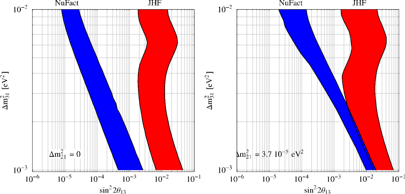
Figure 11: The sensitivity to $\sin^{2}2\theta_{13}$ for the considered JHF and NuFact setups as a function of ${\Delta m^{2}_{31}}$ for ${\Delta m^{2}_{21}}=0$ (left plot) and ${\Delta m^{2}_{21}}=3.7~{}10^{-5}~{}\mathrm{eV}^{2}$ (right plot). The right edge of the NuFact and JHF bands corresponds to the less advanced options, NuFact I and JHF-SK, while NuFact II and JHF-HK are equivalent to the left side of the bands [13].

where we can see that the $\sin^{2}2\theta_{13}$ sensitivity limit depends considerably on the value of ${\Delta m^{2}_{31}}$. From the comparison of the cases ${\Delta m^{2}_{21}}=0$ (left plot) and ${\Delta m^{2}_{21}}=3.7~{}10^{-5}~{}\mathrm{eV}^{2}$ (right plot) we find moreover a significant ${\Delta m^{2}_{21}}$ dependence of the sensitivity limits. The $\sin^{2}2\theta_{13}$ sensitivity limit can thus change considerably depending on what will be found for ${\Delta m^{2}_{31}}$ and ${\Delta m^{2}_{21}}$ and these dependencies are strongest for short baselines.

Assuming that the leading parameters are measured to be ${\Delta m^{2}_{31}}=3\cdot 10^{-3}~{}\mathrm{eV}^{2}$, $\sin^{2}2\theta_{23}=0.8$ and that KamLand measures the solar parameters at the current best fit point of the LMA region, i.e. ${\Delta m^{2}_{21}}=6\cdot 10^{-5}~{}\mathrm{eV}^{2}$ and $\sin 2\theta_{12}=0.91$, we can translate this into a comparison of the $\sin^{2}2\theta_{13}$ sensitivity limit for the different setups. The result is shown in fig. 12. The individual contributions of different sources of uncertainties are shown for every experiment and the left edge of every band in fig. 12 corresponds to the sensitivity limit which would be obtained purely on statistical grounds. This limit is successively reduced by adding the systematical uncertainties of each experiment, the correlational errors and finally the degeneracy errors. The right edge of each band constitutes the final error for the experiment under consideration.

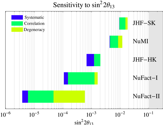
Figure 12: The $\sin^{2}2\theta_{13}$ sensitivity for all setups defined in section 6 at the 90% confidence level for ${\Delta m^{2}_{31}}=3\cdot 10^{-3}\,\mathrm{eV}^{2}$ and $\sin^{2}2\theta_{23}=0.8$. The plot shows the deterioration of the sensitivity limits as the different error sources are successively switched on. The left edge of the bars is the sensitivity statistical limit. This limit gets reduced as systematical, correlational and degeneracy errors are switched on. The right edge is the final sensitivity limit [13].

It is interesting to see how the errors of the different setups are composed. There are different sensitivity reductions due to systematical errors, correlations and degeneracies. The largest sensitivity loss due to correlations and degeneracies occurs for NuFact-II, which is mostly a consequence of the uncertainty of ${\Delta m^{2}_{21}}$, which translates into an $\alpha$ uncertainty, and which dominates the appearance probability eq. (18) for small $\sin^{2}2\theta_{13}$. Note that it is in principle possible to combine different experiments. If done correctly, this allows to eliminate part or all of the correlational and degeneracy errors [61].

It is interesting to recall the existence of the magic baseline discussed in eq. (19), where the $\alpha$ and $\delta$ dependence drops out completely due to matter effects. Correlational and degeneracy errors are then drastically reduced and a measurement of $\sin^{2}2\theta_{13}$ becomes more precise, even though the event rates are smaller at this larger baseline. This improvement in sensitivity is shown for NuFact-II in fig. 13, where a baseline of 3000 km is compared with the magic baseline of $8100~{}\mathrm{km}$.

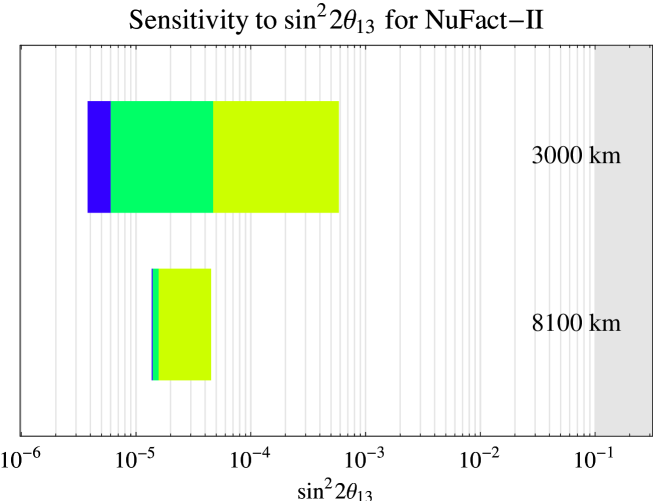
Figure 13: Comparison of the NuFact-II setup for a baseline of 3000 km and the magic baseline of 8100 km. It can be seen that the statistical sensitivity (left edge of the bars) is reduced due to smaller event rates, but the total sensitivity is increased since the correlational and degeneracy errors disappear almost completely at the magic baseline.

Another challenge of future LBL experiments is to measure $sign({\Delta m^{2}_{31}})$ via matter effects and the sensitivity which can be obtained for the setups under discussion is shown in fig. 14.

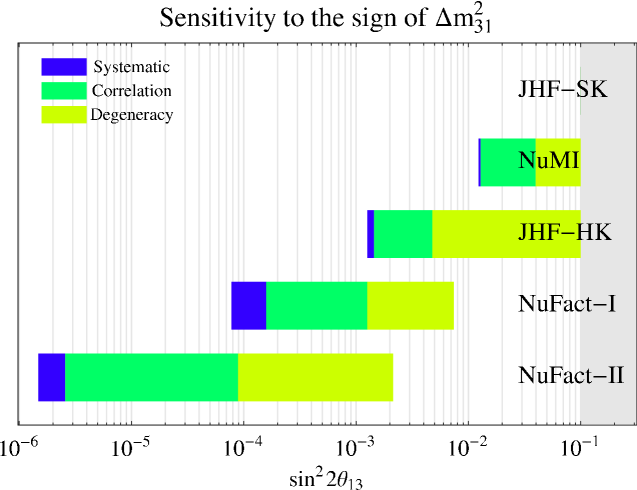
Figure 14: The $\sin^{2}2\theta_{13}$ sensitivity region to $sign({\Delta m^{2}_{31}})$ for the setups defined in section 6. The left edge of the bars are the statistical sensitivity limits which are successively reduced by systematical, correlational and degeneracy errors. The right edge of the bars is the final limit.

Taking all correlational and degeneracy errors into account we can see that it is very hard to determine $sign({\Delta m^{2}_{31}})$ with the considered superbeam setups. The main problem is the degeneracy with $\delta$, which allows always the reversed $sign({\Delta m^{2}_{31}})$ for another CP phase. Note, however, that the situation can in principle be improved if different superbeam experiments were combined such that this degeneracy error could be removed. Neutrino factories perform considerably better on $sign({\Delta m^{2}_{31}})$, particularly for larger baselines. Combination strategies would again lead to further improvements.

Coherent forward scattering of neutrinos and the corresponding MSW matter effects are so far experimentally untested. It is therefore very important to realize that matter effects will not only be useful to extract $sign({\Delta m^{2}_{31}})$, but that they allow also detailed tests of coherent forward scattering of neutrinos. This has been studied in detail in [52, 75, 78, 83].

The Holy Grail of LBL experiments is the measurement of leptonic CP violation.

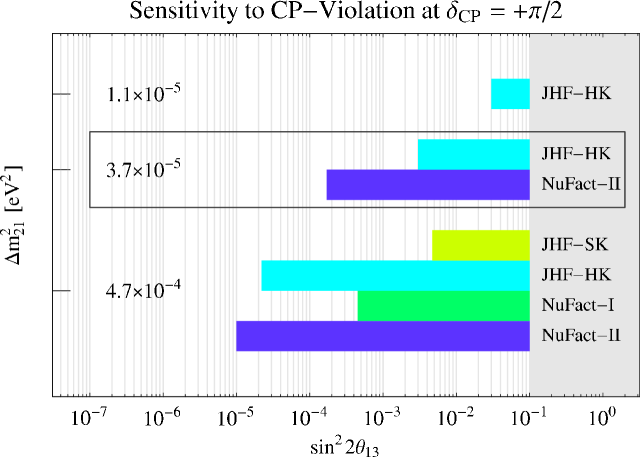
Figure 15: The $\sin^{2}2\theta_{13}$ sensitivity range for CP violation of the considered setups at 90% confidence level and for different $\Delta m_{21}^{2}$ values. The upper row corresponds to the lower bound of $\Delta m_{21}^{2}=1.1\times 10^{-5}~{}\mathrm{eV}^{2}$, the bottom row to the upper bound $\Delta m_{21}^{2}=4.7\times 10^{-4}~{}\mathrm{eV}^{2}$, and the middle row to the best LMA fit, $\Delta m_{21}^{2}=3.7\times 10^{-5}~{}\mathrm{eV}^{2}$. Cases which do not have CP sensitivity are omitted from this plot. The chosen parameters are $\delta=+\pi/2$, ${\Delta m^{2}_{31}}=3\cdot 10^{-3}~{}\mathrm{eV}^{2}$, $\sin^{2}2\theta_{23}=0.8$, and a solar mixing angle corresponding to the current best fit in the LMA regime [13].

The $\sin^{2}2\theta_{13}$ sensitivity range for measurable CP violation is shown in fig. 15 for $\delta=\pi/2$ for the different setups and for different values of ${\Delta m^{2}_{21}}$. It can be seen that measurements of CP violation are in principle feasible both with high luminosity superbeams as well as advanced neutrino factories. However, the sensitivity depends in a crucial way on ${\Delta m^{2}_{21}}$. For a low value ${\Delta m^{2}_{21}}=1.1~{}10^{-5}~{}\mathrm{eV}^{2}$, the sensitivity is almost completely lost, while the situation would be very promising for the largest considered value ${\Delta m^{2}_{21}}=4.7~{}10^{-4}~{}\mathrm{eV}^{2}$. For a measurement of leptonic CP violation it would therefore be extremely exciting and promising if KamLand would find ${\Delta m^{2}_{21}}$ on the high side of the LMA solution (the so-called HLMA case). The sensitivities shown in fig. 15 depend on the choice for $\delta$. The value which was used here was $\delta=\pi/2$ and and the sensitivities become become worse for small CP phases close to zero or $\pi$.

10 Conclusions

We have discussed the potential of certain future long baseline neutrino oscillation experiments, where it will be possible to perform precision neutrino physics. The basic fact which makes this possible is that the atmospheric mass splitting ${\Delta m^{2}_{31}}\simeq\Delta{m^{2}_{\mathrm{atm}}}$ leads for typical neutrino energies $E_{\nu}\simeq 1-100$ GeV to oscillation baselines in the range $100$ km to $10000$ km. Beam sources have moreover the advantage, that unlike the sun or the atmosphere, they can be controlled very precisely, such that unknowns of the neutrino source do not limit the precision. Equally precise detectors and an adequately precise oscillation framework (including three neutrinos and matter effects) must be used in order to exploit this precision. There exist other interesting sources for long baseline oscillation experiments, like reactors or $\beta$-beams, but we restricted the discussion here to superbeams and neutrino factories. We presented the issues which enter into realistic assessments of the potential of such experiments. The discussed experiments turned out to be very promising and they lead to very precise measurements of the leading oscillation parameters ${\Delta m^{2}_{31}}$ and $\sin^{2}2\theta_{23}$. We discussed in detail how the different setups lead to very interesting measurements or limits $\theta_{13}$ and $\delta$. It will also be possible to perform impressive tests of Earth matter effects, allowing to extract $sign({\Delta m^{2}_{31}})$. The discussed setups have an increasing potential and increasing technological challenges, but it seems possible to built them in stages. The shown results are valid for each individual setup and future results should of course be included in the analysis. This would be especially important if more LBL experiments were built and depending on previous results there exist different optimization strategies. In the short run the expected results from KamLand are extremely important and will have considerable impact. First it will become clear if ${\Delta m^{2}_{21}}$ lies in the LMA regime, which is very important since realistically, CP violation can only be measured then. Within the LMA solution it is also very important if ${\Delta m^{2}_{21}}$ lies close to the current best fit, on the high or on the low side. A value of ${\Delta m^{2}_{21}}$ on the high side (HLMA) would be ideal, since it would guarantee an extremely promising LBL program with a chance to see leptonic CP violation already with the JHF beam in the next decade.

Finally we would like to stress that the physics program of LBL experiments has a unique impact on physics. It would lead to very precise neutrino mass splittings and very precise leptonic mixings. These measurements yield directly the physics parameters of interest, which are (unlike quarks) not masked by any hadronic uncertainties. It would thus be possible to get very valuable lepton flavour information, which could be directly compared with models of masses and mixings as well as renormalization group effects. Such precise leptonic flavour information might also proof more valuable than in the quark sector, since neutrino masses receive in general contributions both from Dirac and Majorana mass terms and more might be learned in this way. Leptonic CP violation is also an extremely interesting issue, since it is related to leptogenesis, which is currently the most plausible mechanism to explain the baryon asymmetry of the universe. The experiments which were presented here allow also a number of other studies which have not been discussed here. Some examples are limits on non-standard interactions, FCNC, more than three neutrinos, CPT violation. The results presented here should, however, make clear that oscillation physics with long baseline experiments alone is already very interesting, powerful and important. The realization of the discussed setups is not easy, but it appears possible in stages, guaranteeing a very promising future of neutrino physics.

Acknowledgments: I would like to thank M. Freund, P. Huber and W. Winter for the collaboration in the studies on which this article is based upon. This work was supported by the “Sonderforschungsbereich 375 für Astro-Teilchenphysik” der Deutschen Forschungsgemeinschaft.

References

- [1]
- [2] T. Toshito (SuperKamiokande Collab.), hep-ex/0105023.
-
[3]
Q. R. Ahmad et al. (SNO Collab.),
Phys. Rev. Lett. 89, 011301 (2002),
nucl-ex/0204008. -
[4]
Q. R. Ahmad et al. (SNO Collab.),
Phys. Rev. Lett. 89, 011302 (2002),
nucl-ex/0204009. - [5] V. Barger, D. Marfatia, K. Whisnant and B. P. Wood, Phys. Lett. B537, 179 (2002), hep-ph/0204253.
- [6] A. Bandyopadhyay, S. Choubey, S. Goswami and D. P. Roy, hep-ph/0204286.
- [7] J. N. Bahcall, M. C. Gonzalez-Garcia and C. Peña-Garay, hep-ph/0204314.
- [8] P. C. de Holanda and A. Yu. Smirnov, hep-ph/0205241.
- [9] M. Apollonio et al. (Chooz Collab.), Phys. Lett. B466, 415 (1999), hep-ex/9907037.
- [10] K. Nakamura (K2K Collab.), Nucl. Phys. Proc. Suppl. 91, 203 (2001).
- [11] V. Paolone, Nucl. Phys. Proc. Suppl. 100, 197 (2001).
- [12] A. Ereditato, Nucl. Phys. Proc. Suppl. 100, 200 (2001).
- [13] P. Huber, M. Lindner and W. Winter, hep-ph/0204352.
- [14] L. Wolfenstein, Phys. Rev. D17, 2369 (1978).
- [15] L. Wolfenstein, Phys. Rev. D20, 2634 (1979).
- [16] S.P. Mikheev and A.Y. Smirnov, Sov. J. Nucl. Phys. 42, 913 (1985).
- [17] S.P. Mikheev and A.Y. Smirnov, Nuovo Cim. C9, 17 (1986).
- [18] S. Antusch, J. Kersten, M. Lindner and M. Ratz, hep-ph/0206078.
- [19] S. Antusch, J. Kersten, M. Lindner and M. Ratz, Phys. Lett. B 538, 87 (2002), hep-ph/0203233.
- [20] M. Fukugita and T. Yanagida, Phys. Lett. B 174, 45 (1986).
- [21] W. Buchmuller, hep-ph/0107153, and references therein.
- [22] See e.g. G. C. Branco, R. Gonzalez Felipe, F. R. Joaquim and M. N. Rebelo, hep-ph/0202030.
- [23] E.A. Paschos, hep-ph/0204138.
- [24] F. Arneodo et al., (ICARUS Collab.), Nucl. Instr. Meth. A471, 272 (2000).
- [25] G. Acquistapace et al. (CNGS Collab.) CERN-98-02.
- [26] R. Baldy et al. (CNGS Collab.) CERN-SL-99-034-DI.
- [27] J. Hylen et al. (NuMI Collab.) FERMILAB-TM-2018.
- [28] K. Nakamura (K2K Collab.), Nucl. Phys. A663, 795 (2000).
- [29] Y. Itow et al., hep-ex/0106019.
- [30] M. Aoki, hep-ph/0204008.
- [31] A. Para and M. Szleper, hep-ex/0110032.
-
[32]
See e.g. J.J. Gomez-Cadenas et al.,
(CERN Super Beam working group),
hep-ph/0105297. -
[33]
F. Dydak,
Tech.Rep.,
CERN
(2002),
http://home.cern.ch/dydak/oscexp.ps. - [34] M. Szleper and A. Para, hep-ex/0110001.
- [35] S. Geer, Phys. Rev. D57, 6989 (1998), hep-ph/9712290.
-
[36]
N. Holtkamp and
D. Finley,
Tech. Rep., FNAL
(2002),
http://www.fnal.gov/projects/muon_collider/nu-factory/nu-factory.html -
[37]
Particle Data Group, D.E. Groom et al.,
Eur.Phys.J. C 15,
1 (2000),
http://pdg.lbl.gov/ - [38] A. Blondel et al., Nucl. Instrum. Meth. A451, 102 (2000).
- [39] C. Albright et al., hep-ex/0008064, and references therein.
- [40] P. Zucchelli, hep-ex/0107006.
-
[41]
K. Dick,
M. Freund,
M. Lindner and
A. Romanino,
Nucl. Phys. B 562
(1999) 29, hep-ph/9903308. - [42] F.D. Stacy, Physics of the Earth, edition, John Wiley and Sons, New York, 1977.
- [43] R. J. Geller and T. Hara, hep-ph/0111342.
- [44] E. K. Akhmedov, Sov. J. Nucl. Phys. 47 (1988) 301.
- [45] S. T. Petcov, Phys. Lett. B 434 (1998) 321, hep-ph/9805262.
- [46] E.K. Akhmedov, Nucl. Phys. B 538, 25 (1999), hep-ph/9805272.
- [47] M. V. Chizhov, S. T. Petcov, Phys. Rev. Lett. 83 (1999) 1096, hep-ph/9903399.
- [48] M. V. Chizhov, S. T. Petcov, Phys. Rev. D 63 (2001) 073003, hep-ph/9903424.
- [49] E.K. Akhmedov, Phys. Atom. Nucl. 64, 787 (2001) [Yad. Fiz. 64, 851 (2001)], hep-ph/0008134.
- [50] A. Cervera et al., Nucl. Phys. B579, 17 (2000), erratum ibid., Nucl. Phys. B593, 731 (2001), hep-ph/0002108.
- [51] M. Freund, Phys. Rev. D64, 053003 (2001), hep-ph/0103300.
-
[52]
M. Freund,
P. Huber, and