hep-ph/0612124 DESY 06-225 SFB/CPP-06-56

Two-Loop Renormalization in the Standard Model
Part III: Renormalization Equations and their Solutions

Stefano Actis

Deutsches Electronen - Synchrotron, DESY, Platanenallee 6, 15738 Zeuthen, Germany

Giampiero Passarino

Dipartimento di Fisica Teorica, Università di Torino, Italy
INFN, Sezione di Torino, Italy

In part I and II of this series of papers all elements have been introduced to extend, to two loops, the set of renormalization procedures which are needed in describing the properties of a spontaneously broken gauge theory. In this paper, the final step is undertaken and finite renormalization is discussed. Two-loop renormalization equations are introduced and their solutions discussed within the context of the minimal standard model of fundamental interactions. These equations relate renormalized Lagrangian parameters (couplings and masses) to some input parameter set containing physical (pseudo-)observables. Complex poles for unstable gauge and Higgs bosons are used and a consistent setup is constructed for extending the predictivity of the theory from the Lep1 $Z$-boson scale (or the Lep2 $WW$ scale) to regions of interest for LHC and ILC physics.

Key words: Feynman diagrams, Multi-loop calculations, Vertex diagrams

PACS Classification: 11.10.-z, 11.15.Bt, 12.38.Bx, 02.90.+p, 02.60.Jh, 02.70.Wz

1 Introduction

The end of the Lep period represented a moment of transition in the development of techniques designed for producing high precision results for collider physics.

It is a well known fact that the advent of a new hadronic machine, the LHC in this case, gives a privileged role to QCD but what is the real implication of this fact?

QCD is a theory devoted to studying strong interactions by means of perturbative methods, a road which has been made possible by the discovery of asymptotic freedom. It is a theory with very few scales and therefore its perturbative aspects are technically simpler. For this reason most of the new ideas are, first of all, tested in QCD where we have an extensive literature of explicit results up to four-loop Feynman diagrams. The very recent twistor spinoff for collider physics [1] has its immediate target in the realm of QCD going beyond the traditional field-theoretic point of view.

Generally speaking we are now witnessing the development of three parallel roads: techniques (mostly Monte Carlo driven [2] or twistor inspired [3]) to deal with tree level processes with many particles in the final state; complete one-loop calculations for $2\to 4$ processes with a particular emphasis on the proper treatment of intermediate unstable particles [4] and genuine electroweak two-loop calculations of physical observables ([5] and [6]), including supersymmetric effects [7]. The first item in the list is deeply linked to the LHC physic programme and has already collected a sizable number of important results. Extension of one-loop calculations to four particles in the final state represents a bridge between LHC and LC physics while two-loop electroweak physics is, at the moment, in some early stage of development. It is worth mentioning, however, that past history has told us about the importance of a complete calculation when dealing with the final analysis of the experimental data.

Lep1 physics has ben mostly dealing with $2\to 2$ processes, where one has been able to assemble the most complete set of predictions in the whole history of radiative corrections. Most notable is the fact that the technology needed for the operation has been pushed well beyond what was expected at the beginning of the period, very much as in the case of the experimental analysis. The key ingredients have been

• the construction of a complete one-loop renormalization procedure for the standard model [8], with the inclusion of several leading and next-to-leading higher order effects;

• the development of libraries for assembling the relevant one-loop diagrams, including reduction of tensor integrals to scalar ones and analytical evaluation of the latter [9];

• inclusion of higher-order, real and virtual, QED effects [10];

• development of fitting procedures to deal with pseudo and realistic experimental observables.

At the very end of the Lep period it became evident that these procedures should be generalized if we want to have a full two-loop interpretation of the data. Furthermore, it became obvious that a step forward is necessary for treating the technological elements which are mandatory in obtaining a satisfactory solution to all the items of our wish-list. There are several aspects which deserve a specific comment: the main one can be summarized by saying that assembling a two-loop package is not, anymore, a one-man-show as it was in the past but requires instead a dedicated involvement of a well coordinated group.

There are many new aspects in the project that put an unprecedented challenge: for any multi-scale process we have to abandon the fully analytical way and new, numerical, algorithms must be developed to handle the complexity of Feynman diagram evaluation with cutting-edge calculations. Generally speaking we are referring here to the evaluation of master integrals, a minimal set of diagrams to which all other diagrams are reduced. The techniques for reduction should be general enough to handle three or more external legs in a fully massive world. On top of that one should not forget to develop a comprehensive two-loop renormalization procedure, flexible enough to be implemented in practice.

What we are describing here is a multi-step program and only one of the steps will be presented in this paper; to fully understand the results, however, it is important to mention that everything has been developed in parallel and what we are going to illustrate is already fitting in the general layout of our program. The general strategy for handling multi-loop, multi-leg Feynman diagrams was designed in [11] and the collection of results necessary for evaluating two-loop, two-point integrals can be found in ref. [12]. Next the calculation of two-loop three-point scalar integrals: infrared-convergent configurations are discussed in [13] and infrared- and collinear-divergent ones are analyzed in [14]. Finally, our method for dealing with two-loop tensor integrals can be found in [15] and results for one-loop multi-leg integrals are shown in [16].

First of all, we needed a technique for reducing diagrams to some set of master integrals. Here, we are referring to a class of two-loop calculation with few external legs, avoiding the exponential complexity that would be encountered with many legs. This step requires our ability in treating all relevant limits, when masses are negligible or when external momenta must be set to zero. We should mention that the real world is massive, with all masses different, but most of them negligibly small. To mention an important aspect we may say that any numerical treatment that does not extract collinear and Sudakov logarithms from the very beginning is doomed to failure. Furthermore, all the results must be stored in the most appropriate form, since our final numerical integration must be absolutely stable.

Next, a full two-loop renormalization had to be designed and we have to make clear the meaning of this sentence. Diagrams have to be generated with some automatic procedure; in our project, we did not want to rely on any black box, so we have constructed our own set of procedures, creating the ${\cal G}raph{\cal S}hot$ package [17].

After assembling diagrams we wanted to perform all sort of canonical tests which, essentially, amounts to check all possible unrenormalized WST identities. After checking that everything has been properly assembled we have been moving to the next logical step, removing all ultraviolet infinities. At the very end one has to admit that the removal is a simple business but we pretend having done it in the most rigorous way. To mention an example we quote the problem of overlapping divergencies; non-local residues of ultraviolet poles must cancel in the total if unitarity of the theory has to be preserved: it is highly non trivial but they indeed do cancel. After that one has to check renormalized WST identities.

Removing ultraviolet poles means trading bare parameters for renormalized ones and, after that, renormalization equations must be written and solved which is equivalent to express theoretical predictions in terms of an input parameter set. In this paper, we illustrate the role of the running e.m. coupling constant and give a full account of the calculation of the Fermi coupling constant.

Another, non trivial, aspect of our work is related to proving that what we expect to vanish is indeed zero; for instance one can prove that the standard model can be made, to some extent, QED-like: at the level of S-matrix elements we expect that vertices, with the inclusion of wave-function factors, do not contribute to the renormalization of the electric charge. To prove this property at two loops is far from trivial.

It is by now clear that one cannot produce all the results in a two-loop calculation without having a software package, ${\cal G}raph{\cal S}hot$ [17] in our case; ${\cal G}raph{\cal S}hot$ collects all the relevant algorithms. At this stage the package is far from being user friendly (for instance we even miss a user’s guide) and it is not even clear if somebody else will use it but writing the code has been an essential step without which none of the results presented in this paper would have been achieved. Once more, past experience is telling us that with the present level of complexity there will be no time, in a few years, to go back and to allow for extensions which were not foreseen from the very beginning.

To summarize, we have performed several steps towards complete two-loop renormalization in the standard model, steps that could be easily generalized, with few minor adjustments, to an arbitrary renormalizable quantum field theory. The introductory elements have been given in [18] (hereafter I) and in [19] (hereafter II).

As it is well known, finite $S$-matrix elements can be obtained without the explicit use of counterterms, a fact that has been fully described in the one-loop renormalization [10]. However, most of the people are more familiar with the language of counterterms and, for this reason, we have decided to adapt our approach. In part II we have described the strategy for making the one- and two-loop Green functions of the theory ultraviolet finite; this amounts to rewrite the Lagrangian in terms of renormalized quantities.

The next step in our procedure will be to express renormalized parameters in terms of physical observables belonging to some input parameter set (hereafter, IPS). In any one-loop calculation one tries to improve upon the accuracy of the result by including leading (and even next-to-leading) higher order effects (which are often available in analytical form) and by performing resummations which, quite often, cannot be fully justified. Here we focus on the issue of setting up a complete two-loop calculus, postponing the question of building improved two-loop resummations.

At two loops we have a new feature, as described in details by many authors: the use of on-shell mass renormalization is not allowed anymore and complex poles are the only meaningful quantities: a property of the $S\,$-matrix, as it is often stated [20]. A better argument is that complex poles are gauge parameter independent to all orders, as shown by using Nielsen identities [21].

Renormalization with complex poles should not be confused with a simple recipe for the replacement of running widths with constant widths; there are many more ingredients in the scheme. Actually, this scheme allows for the introduction of a beautiful language, the one of effective (complex) couplings. The whole organization of loop corrections is most conveniently organized in terms of running couplings, as illustrated by the development of the fermion loop approximation. Unfortunately gauge invariance – the ingredient at the basis of the successful proof of renormalization – prevents us from fully extending the use of running, resummed, couplings to the bosonic sector of the theory (as a matter of fact even the concept of a fermionic sector is meaningless abeyond one loop). Despite this caveat we will organize the presentation of our results according to the language of running couplings; in a way this language is much easier and one should only remember that final results must be expanded in perturbation theory up to second order. Partial resummations, i.e. the attempt of isolating gauge parameter independent blocks that can be moved freely from numerators to denominators is beyond the scope of this paper.

Neglecting the fine points of the procedure we may say that the transition from renormalized parameters to physical quantities depends on the choice of the latter. Quantities like $G_{{\scriptscriptstyle{F}}}$ and $\alpha$, the Fermi coupling constant and the fine structure constant, will always be included in our choice of the IPS. For most of the cases under consideration fermion masses and the Higgs boson mass are only needed at one loop; here on-mass-shell masses can be used. For gauge bosons instead, we have to extract from the data some information about the position of the corresponding complex poles. The fact that we still indulge in presenting theoretical prediction for, say $M_{{}_{W}}$, is a consequence of an established attitude that every pseudo-observable can be defined and derived from data, although its theoretical degree of purity is vanishing small. To an even larger extent the situation with the Higgs boson mass (as used in any LHC Monte Carlo program) is fully unclear.

Having adopted this strategy, we may say that the final step in renormalization can still be seen as the moment where we write a system of (essentially) three coupled equations, relating $g,s_{\theta}$ and $M$ (all renormalized quantities) to $G_{{\scriptscriptstyle{F}}},\alpha,\,\dots$.

In this paper, we shall follow the same notations as defined in our companion papers I and II. We therefore refer the reader to that papers for notations; in particular, $M$ stands for the bare (renormalized) $W$ boson mass (we do not distinguish unless strictly needed), $M_{0}=M/c_{\theta}$ where $c_{\theta}$ is the bare (renormalized) cosine of the weak-mixing angle; $M_{{}_{W}}$ is the on-shell $W$ boson mass and $M_{{}_{Z}}=M_{{}_{W}}/c_{\theta}$.

The outline of the paper is as follows: in Section 2 we summarize our procedure, and in Section 3 we present a renormalization equation based on the use of the Fermi coupling constant; aspects of the calculation connected with the proper definition of $\gamma^{5}$ are discussed in Section 4. A second renormalization equation connected with the fine structure constant is analyzed in Section 5. The running of $\alpha$ beyond one-loop fermion terms is discussed in Section 6. Complex poles are introduced in Section 7 and solutions of the renormalization equations in Section 8. Loop diagrams with dressed propagators are introduced in Section 9, unitarity, gauge parameter independence and WST identities in Section 10. A suggestion on how to improve the complex mass scheme [4] is finally introduced in Section 11.

2 Outline of the calculation

Figure 1: Renormalization - flowchart. Feynman rules define the theory, renormalizability guarantees that ultraviolet poles have polynomial residues and can be subtracted. Any input parameter set allows us to replace renormalized quantities with experimental data. A prediction follows.

The whole renormalization procedure has been summarized in the flowchart of Fig. 1 where IPS stands for Input Parameter Set. Object of this paper is to introduce renormalization equations (RE) and to solve them, therefore undertaking the task of writing any (pseudo-)observable, not in the IPS, in terms of the quantities of the IPS. The minimal standard model is essentially a three-parameter theory and therefore we seek for a system of three (coupled) REs whose unknowns are $g,M$ and $s_{\theta}$, all renormalized parameters. In Section 3 we discuss the first RE, related to the Fermi coupling constant, $G_{{\scriptscriptstyle{F}}}$. In Section 5 we present the second RE, related to fine structure constant $\alpha$. In Section 7 we introduce the third RE, based on the notion of complex pole for unstable gauge bosons. The solution of our RE is discussed in Section 8 where we present two choices for the IPS.

3 The Fermi-coupling constant

In this section we present the results for $G_{{\scriptscriptstyle{F}}}$. A critical observation is that writing a renormalization equation for the Fermi-coupling constant should not be confused with predicting the muon lifetime or the Fermi coupling constant itself (also in an effective field-theory approach, see i.e. Ref. [22]).

To proceed further, we illustrate our method for relating the $\overline{MS}$-renormalized parameters of the Standard Model to the Fermi coupling constant at two loops and we construct our first renormalization equation.

The Fermi coupling constant, $G_{{\scriptscriptstyle{F}}}$, is defined by

$$\frac{1}{\tau_{\mu}}\,=\,\frac{G_{{\scriptscriptstyle{F}}}^{2}\,m_{\mu}^{5}}{192\,\pi^{3}}\,(\,1\,+\,\Delta q\,),$$ (1)

where $\tau_{\mu}$ and $m_{\mu}$ are the observed muon lifetime and mass. The parameter $\Delta q$ summarizes both real and virtual corrections to $\tau_{\mu}$, at leading order in $G_{{\scriptscriptstyle{F}}}$ and to all orders in the fine-structure constant $\alpha$. The corrections are generated by the effective Lagrangian

$${\cal L}_{\rm{\scriptscriptstyle{QED}}\times\rm{\scriptscriptstyle{FT}}}\,=\,{\cal L}_{\rm{\scriptscriptstyle{FT}}}\,+\,{\cal L}_{\rm{\scriptscriptstyle{QED}}},\qquad{\cal L}_{{}_{\rm{\scriptscriptstyle{FT}}}}\,=\,\frac{G_{{\scriptscriptstyle{F}}}}{\sqrt{2}}\,\,\,\,\left[\,{\overline{\nu}}_{\mu}\,\gamma_{\alpha}\,\left(1+\gamma_{5}\right)\,\mu\,\right]\,\,\cdot\,\,\left[\,{\overline{e}}\,\gamma_{\alpha}\,\left(1+\gamma_{5}\right)\,\nu_{e}\,\right].$$ (2)

Here ${\cal L}_{\rm{\scriptscriptstyle{FT}}}$ describes the contact-interaction Fermi theory (FT), ${\cal L}_{\rm{\scriptscriptstyle{QED}}}$ is the usual QED Lagrangian and $\mu$, $e$, $\nu_{\mu}$ and $\nu_{e}$ are the spinor fields for the muon, the electron and their related neutrinos.

The inclusion of electromagnetic effects allows to determine the numerical value of $G_{{\scriptscriptstyle{F}}}$ in terms of the measurable quantities $\tau_{\mu}$, $\alpha$, $m_{\mu}$ and the electron mass $m_{e}$. The combination of the one-loop [23] and two-loop [24] QED$\,\times\,$FT contributions with the non-perturbative hadronic components [25] leads to estimate

$$G_{{\scriptscriptstyle{F}}}\,=\,(1.16637\,\pm\,0.00001)\,\times 10^{-5}\,\mathrm{GeV}^{-2}.$$ (3)

Unfortunately, another definition is often employed in the literature (see e.g. Ref. [26]),

$$\frac{1}{\tau_{\mu}}\,=\,\frac{G_{{\scriptscriptstyle{F}}}^{2}\,m_{\mu}^{5}}{192\,\pi^{3}}\,(\,1\,+\,\Delta q\,)\,\,F\left(\frac{m_{e}^{2}}{m_{\mu}^{2}}\right)\,\,\left(\,1\,+\,\frac{3}{5}\,\frac{m_{\mu}^{2}}{M_{{\scriptscriptstyle{W}}}^{2}}\,\right),$$ (4)

where $M_{{\scriptscriptstyle{W}}}$ is the $W$-boson mass and $F(m_{e}^{2}/m_{\mu}^{2})$ follows from the phase-space integration at lowest order in perturbation theory,

$$F(x)\,=\,1-8\,x-12\,x^{2}\,\ln x+8\,x^{3}-x^{4}.$$ (5)

However, the factor $(1+3m_{\mu}^{2})/(5M_{{\scriptscriptstyle{W}}}^{2})$ is the tree-level $W$-propagator effect and is not generated by the Fermi-contact interaction. Moreover, as pointed out by the authors of Ref. [24], the function $F$ does not factorize in the same way at higher orders. Therefore, in order to avoid unnecessary ambiguities, we will use the definition of Eq.(1).

In the context of our renormalization procedure, $G_{{\scriptscriptstyle{F}}}$ is an input data and we have to derive the appropriate renormalization equation. First we express $\tau_{\mu}$ through the SM renormalized parameters. Next, we match our result with the definition of Eq.(1) getting a relation between a measurable quantity, $G_{{\scriptscriptstyle{F}}}$, and the SM renormalized parameters,

$$\frac{G_{{\scriptscriptstyle{F}}}}{\sqrt{2}}\,=\,\frac{g^{2}}{8\,M^{2}}\,(\,1\,+\,\Delta g\,).$$ (6)

Here $g$ and $M$ are the renormalized weak-coupling constant and $W$-boson mass and the quantity $\Delta g$ is constructed order-by-order through the purely-weak corrections to the muon lifetime. Electromagnetic components are already included in Eq.(1) and they are discarded through the matching procedure.

It is worth noting that the answer for $\Delta g$ will contain renormalized parameters and counterterms. The choice of the renormalization scheme determines the explicit expressions for the counterterms and the final result for $\Delta g$. A popular strategy, followed in recent two-loop calculations of the muon-decay width [27, 28], is to employ the on-mass-shell (OMS) scheme and to define renormalized parameters by means of measurable quantities. At lowest order one has simple relations,

$$e^{2}=g^{2}s_{\theta}^{2}=4\pi\,\alpha,\qquad c_{\theta}^{2}=\frac{M^{2}_{{}_{W}}}{M^{2}_{{}_{Z}}},\qquad M=M_{{}_{W}}.$$ (7)

Here $e$ is the renormalized electric charge, $M_{{}_{W}}$ and $M_{{}_{Z}}$ are the on-shell masses of the $W$ and $Z$ bosons and $c_{\theta}$($s_{\theta}$) is the renormalized cosine (sine) of the weak-mixing angle. A replacement of the OMS renormalization prescription into Eq.(6) leads to the traditional parametrization employed to describe the interdependence between the masses of the vector bosons introduced in Ref. [29].

Rather that defining exactly what the renormalized parameters are, like in Eq.(7), we prefer to follow a minimal-subtraction scheme. Let us prescribe the values of the counterterms as an intermediate step to remove ultraviolet poles and regularization-dependent factors. Relations among renormalized parameters and physical quantities are not imposed by hand and represent the solution of the chosen set of renormalization equations. Therefore, our result for $\Delta g$ should not be confused with $\Delta r$ as reported by the authors of Ref. [27, 28].

The basic prerequisite to derive the renormalization equation for $G_{{\scriptscriptstyle{F}}}$ is the extraction of the QED$\,\times\,$FT components from the full SM calculation of the muon lifetime. In Subsection 3.1 we discuss our method and detail the result with some relevant diagrammatic examples. Note that the definition of $G_{{\scriptscriptstyle{F}}}$ relegates the infrared structure of muon decay to the soft electromagnetic effects summarized by $\Delta q$ in Eq.(1) and does not affect the hard weak remainder, $\Delta g$.

Moreover, in our approach, external legs will be provided with appropriate wave-function renormalization (WFR) factors; since most of the existing literature deals with the OMS scheme, where WFR factors are usually replaced by field counterterms, we devote Subsection 3.2 to discuss their role. Of course, the connection between field renormalization and wave-function factors is well understood, they are simply connected by a field transformation.

Finally, in Subsection 3.3 and Subsection 3.4, we give our results for $\Delta g$ at one loop (consistency check) and at two loops.

3.1 Extraction of the electromagnetic components

In this subsection we consider the Standard Model tree-level amplitude for muon-decay and fix our notations an conventions. The process is

$$\mu(p_{1})\,\to\,\nu_{\mu}(p_{2})\,+\,e(p_{3})\,+\,{\overline{\nu}}_{e}(p_{4}).$$ (8)

Neglecting the electron mass and the squared momentum carried by the intermediate $W$-boson propagator, the result in ’t Hooft-Feynman gauge reads as

$${\cal M}^{0}\,=\,-\,(2\pi)^{4}\,i\,\frac{g^{2}}{8\,M^{2}}\,\,\,\left[\,{\overline{u}}_{2}\,\gamma_{\alpha}\,\left(1+\gamma_{5}\right)\,u_{1}\,\right]\,\cdot\,\left[\,{\overline{u}}_{3}\,\gamma_{\alpha}\,\left(1+\gamma_{5}\right)\,v_{4}\right],$$ (9)

where we used the short-hand notation for spinors $u_{i}=u(p_{i})$ and $v_{i}=v(p_{i})$.

The key observation is that the QED corrections in the context of the Fermi-contact interaction can be systematically identified and removed from the full SM amplitude. The one-loop matrix element factorizes as

$${\cal M}^{1L}\,=\,{\cal M}^{0}\,\,\left(\,1\,+\,\Delta{\cal M}^{1L}_{\rm{\scriptscriptstyle{QED}}\times\rm{\scriptscriptstyle{FT}}}\,\right)\,\,\left(\,1\,+\,\Delta{\cal M}^{1L}_{\rm{\scriptscriptstyle{WEAK}}}\,\right)\,+{\cal O}\left(g^{6}\right),$$ (10)

where $\Delta{\cal M}^{1L}_{\rm{\scriptscriptstyle{QED}}\times\rm{\scriptscriptstyle{FT}}}$ is a scalar function which summarizes all the QED$\,\times\,$FT soft contributions and the purely-weak remainder is entirely relegated to the hard component $\Delta{\cal M}^{1L}_{\rm{\scriptscriptstyle{WEAK}}}$. At two loops the amplitude can be decomposed as

$${\cal M}^{2L}\,=\,{\cal M}^{0}\,\,\left(\,1\,+\,\Delta{\cal M}^{1L}_{\rm{\scriptscriptstyle{QED}}\times\rm{\scriptscriptstyle{FT}}}\,+\,\Delta{\cal M}^{2L}_{\rm{\scriptscriptstyle{QED}}\times\rm{\scriptscriptstyle{FT}}}\,\right)\,\,\left(\,1\,+\,\Delta{\cal M}^{1L}_{\rm{\scriptscriptstyle{WEAK}}}\,+\,\Delta{\cal M}^{2L}_{\rm{\scriptscriptstyle{WEAK}}}\right)\,+{\cal O}\left(g^{8}\right),$$ (11)

where $\Delta{\cal M}^{2L}_{\rm{\scriptscriptstyle{QED}}\times\rm{\scriptscriptstyle{FT}}}$ and $\Delta{\cal M}^{2L}_{\rm{\scriptscriptstyle{WEAK}}}$ denote two-loop soft and hard corrections. The class of soft effects generates the parameter $\Delta q$ of Eq.(1). We discard them and we identify the hard terms with the quantity $\Delta g$ introduced in Eq.(6),

$$\Delta g\,=\,\Delta{\cal M}^{1L}_{\rm{\scriptscriptstyle{WEAK}}}\,+\,\Delta{\cal M}^{2L}_{\rm{\scriptscriptstyle{WEAK}}}\,+{\cal O}\left(g^{6}\right).$$ (12)

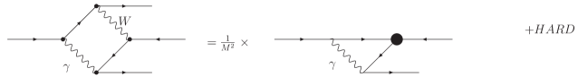
Figure 2: Diagrammatic interpretation of Eq.(13). The first graph is a box diagram in the full SM context. The one-photon vertex diagram is a QED correction in the Fermi-contact interaction, denoted by the black circle.

A simple one-loop example shows how the QED$\,\times\,$FT components factorize in the SM amplitude. We apply the procedure introduced in Ref. [30] to separate off the soft electromagnetic corrections from the hard remainder in the SM box diagram of Fig. 2. If $q$ denotes the momentum of the virtual photon and $q+p$ the momentum flowing through the $W$-boson line, we decompose the integrand in the large $W$-mass limit,

$$\frac{1}{q^{2}\,[\,(q+p)^{2}+M^{2}\,]}=\frac{1}{M^{2}}\,\,\Bigl{(}\,\frac{1}{q^{2}}-\frac{1}{q^{2}+M^{2}}\,\Bigr{)}\,\Bigl{(}\,1\,-\,\frac{2q\cdot p+p^{2}}{q^{2}+M^{2}}+\ldots\,\Bigr{)}.$$ (13)

Here the first term generates the soft QED-vertex correction to the local Fermi interaction of Fig. 2, which can be obtained replacing the $W$-boson propagator by $1/M^{2}$. We discard this component and we evaluate the hard weak remainder in the large vector-boson mass limit, where the external momenta and the lepton masses can be safely neglected,

$${{\cal M}}^{{\scriptscriptstyle{W}}\gamma}_{\rm{\scriptscriptstyle{WEAK}}}=\frac{g^{4}\,s_{\theta}^{2}}{8\,M^{2}}\,\mu^{4-n}\,\int d^{n}q\,\frac{q_{\mu}\,q_{\nu}}{(q^{2})^{2}(q^{2}+M^{2})}\,\Gamma_{\mu\nu}^{{{\scriptscriptstyle{W}}\gamma}}.$$ (14)

Here $\mu$ is the ’t Hooft unit of mass and the spinor chain reads as

$$\Gamma^{{{\scriptscriptstyle{W}}\gamma}}_{\mu\nu}\,\equiv\,\left[\,{\overline{u}}_{2}\,\gamma_{\alpha}\,\gamma_{+}\,\gamma_{\mu}\,\gamma_{\beta}\,u_{1}\,\right]\,\,\cdot\,\,\left[\,{\overline{u}}_{3}\,\gamma_{\beta}\,\gamma_{\nu}\,\gamma_{\alpha}\,\gamma_{+}\,v_{4}\,\right],$$ (15)

where $\gamma_{\pm}=1\pm\gamma^{5}$. Note that the purely-weak components can be obviously obtained starting from the full SM amplitude and subtracting the QED$\,\times\,$FT terms. Therefore, instead of extracting the hard correction from the box diagram of Fig. 2, we can use an alternative strategy:

I) We construct the difference of the box diagram and the QED$\,\times\,$FT component of Fig. 2. This can be evaluated nullifying the external momenta and the lepton masses.

II) Here the soft electromagnetic term is a massless tadpole which vanishes in dimensional regularization. With a non-zero electron mass, of course, it develops infrared and collinear singularities. Therefore, any information about the infrared structure is lost but these effects are already included in $\Delta q$ of Eq.(1) and are not relevant for $\Delta g$.

III) As a result, the hard part follows directly from the complete one-loop diagram by nullifying the lepton masses and the external momenta,

$${{\cal M}}^{{\scriptscriptstyle{W}}\gamma}_{\rm{\scriptscriptstyle{WEAK}}}=-\frac{g^{4}\,s_{\theta}^{2}}{8}\,\mu^{4-n}\,\int d^{n}q\,\frac{q_{\mu}q_{\nu}}{(q^{2})^{3}(q^{2}+M^{2})}\,\Gamma_{\mu\nu}^{{\scriptscriptstyle{W}}\gamma}.$$ (16)

Using the fact that in dimensional regularization an integral without scales is zero it is easy to see that the two representations of Eq.(14) and Eq.(16) are completely equivalent. Since QED factorization should not be proven by assumption, and one has anyway to separate off the QED$\,\times\,$FT components, the choice between the two procedures is just a matter of taste. However, the subtraction method of Eq.(16), introduced in Ref. [28], appears more appropriate in the context of an automatic approach, where all the Feynman diagrams are generated and evaluated by neglecting the soft scales from the very beginning.

The matching on the Fermi-theory spinor-chain configuration can be finally completed when we introduce the projector,

$${\cal P}\,=\,\sum_{\rm{spins}}\,\left[\,{\overline{v}}_{4}\,\gamma_{\lambda}\,\gamma_{+}\,u_{2}\,\right]\,\,\cdot\,\,\left[\,{\overline{u}}_{1}\,\gamma_{\lambda}\,\gamma_{+}\,u_{3}\,\right]$$ (17)

which will act on the matrix element for muon decay. For example, for the hard part of Eq.(14) we can write

$${\cal M}^{{\scriptscriptstyle{W}}\gamma}_{\rm{\scriptscriptstyle{WEAK}}}={\cal M}^{0}\,\,\cdot\,\,\Delta{\cal M}^{{\scriptscriptstyle{W}}\gamma}_{\rm{\scriptscriptstyle{WEAK}}},\quad\mbox{with}\quad\Delta{\cal M}^{{\scriptscriptstyle{W}}\gamma}_{\rm{\scriptscriptstyle{WEAK}}}=\frac{{\cal P}{\cal M}^{{\scriptscriptstyle{W}}\gamma}_{\rm{\scriptscriptstyle{WEAK}}}}{{\cal P}{\cal M}^{0}}.$$ (18)

Two-loop virtual corrections to the muon-decay amplitude can be classified according to Fig. 3.

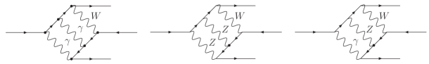
Figure 3: Two-loop box diagrams for muon decay.

Here diagram a) contains two photons and one hard scale and can be treated in complete analogy with the one-loop case. After shrinking the heavy line to a point like in Fig. 4, the two-photon graph in the local Fermi theory is discarded. The hard weak remainder is obtained by nullifying the soft scales in the full two-loop box diagram.

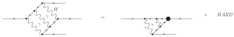
Figure 4: Two-loop soft $\otimes$ soft splitting.

Diagram b) includes just heavy components, and does not require any subtraction. We will evaluate it in the soft limit obtaining a finite answer.

Since in diagram c) soft and hard components are entangled, we discuss it in more detail. We consider the subloop with a photon and a $Z$ boson and we decompose it in the large $Z$-boson mass limit. If $q_{1}$ is the momentum flowing along the photon line and $q_{1}-q_{2}$ is the momentum of the $Z$ propagator, we can write

$$\frac{1}{q_{1}^{2}\,[\,(q_{1}-q_{2})^{2}+M_{0}^{2}\,]}=\frac{1}{q_{1}^{2}}\,\frac{1}{q_{2}^{2}+M_{0}^{2}}\,\,\,\Bigl{(}\,1\,+\,\frac{2q_{1}\cdot q_{2}-q_{1}^{2}}{q_{2}^{2}+M_{0}^{2}}+\ldots\,\Bigr{)},$$ (19)

where $M_{0}=M/c_{\theta}$. The first term gives the product of a one-loop QED$\,\times\,$FT vertex and a one-loop weak remainder, as shown in Fig. 5.

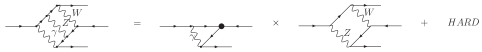
Figure 5: Two-loop soft $\otimes$ hard splitting.

The rest is a purely-weak two-loop component which will be evaluated after nullification of external momenta and lepton masses.

The soft$\,\times\,$hard term is crucial in proving the two-loop factorization property of Eq.(11), because it generates the $\Delta{\cal M}^{1L}_{\rm{\scriptscriptstyle{QED}}\times\rm{\scriptscriptstyle{FT}}}\times\Delta{\cal M}^{1L}_{\rm{\scriptscriptstyle{WEAK}}}$ part. To evaluate the hard remainder, we start again from the complete representation for the SM diagram, where we nullify the soft scales,

$${\cal M}^{{\scriptscriptstyle{W}}{\scriptscriptstyle{Z}}\gamma}_{\rm{\scriptscriptstyle{WEAK}}}\,=\,-\,\frac{1}{(2\pi)^{4}\,i}\,\frac{1}{32}\,\frac{g^{2}\,s_{\theta}^{2}}{c_{\theta}^{2}}\,\mu^{2(4-n)}\,\int d^{n}q_{1}d^{n}q_{2}\,\frac{q_{1\delta}\,q_{2\nu}\,q_{1\rho}\,q_{2\sigma}}{(q_{1}^{2})^{3}\,(q_{2}^{2})^{2}\,(q_{2}^{2}+M^{2})\,[(q_{1}-q_{2})^{2}+M_{0}^{2}]}\,\,\Gamma^{{\scriptscriptstyle{W}}{\scriptscriptstyle{Z}}\gamma}_{\delta\nu\rho\sigma}.$$ (20)

Here the spinor chain reads as

$$\Gamma^{{\scriptscriptstyle{W}}{\scriptscriptstyle{Z}}\gamma}_{\mu\nu\rho\sigma}\,=\,\left[\,{\overline{u}}_{2}\,\gamma_{\alpha}\,\gamma_{+}\,\gamma_{\nu}\,\gamma_{\beta}\,(v_{\mu}+a_{\mu}\gamma_{5})\,\gamma_{\delta}\,\gamma_{\gamma}\,u_{1}\,\right]\,\,\cdot\,\,\left[\,{\overline{u}}_{3}\,\gamma_{\gamma}\,\gamma_{\rho}\,\gamma_{\beta}\,(v_{e}+a_{e}\gamma_{5})\,\gamma_{\sigma}\,\gamma_{\alpha}\,\gamma_{+}\,v_{4}\,\right]$$ (21)

and $v_{f}=I_{f}^{(3)}-2Q_{f}^{2}s_{\theta}^{2}$ and $a_{f}=I_{f}^{(3)}$, where $I_{f}^{(3)}$ is the weak-isospin third component for the fermion $f$ and $Q_{f}$ is the related electric-charge quantum number. Finally, a correct description of muon decay involves also real radiative effects. This is essential in showing that the QED$\,\times\,$FT corrections are finite [23, 24] and allows to define the Fermi-coupling constant through Eq.(1). Nevertheless, one can easily prove that real soft-radiation diagrams can be systematically neglected from the calculation.

3.2 Wave-function renormalization factors

Wave-function renormalization factors for external legs (hereafter WFR) contain derivatives of two-point Green’s functions which are infrared divergent and deserve a special discussion. In order to derive explicit representations for the muon-decay case we consider the fermion one-particle irreducible Green’s function,

$$\Sigma(p)\,=\,(2\pi)^{4}\,i\,\,\left\{\,a_{{\scriptscriptstyle{S}}}(p^{2})\,+\,\left[\,a_{{\scriptscriptstyle{V}}}(p^{2})\,-\,a_{{\scriptscriptstyle{A}}}(p^{2})\,\gamma_{5}\,\right]\,i\,/\!\!\!p\,\right\},$$ (22)

where we introduced a scalar, a vector and an axial form factor (the SM pseudo-scalar component obviously vanishes). The fermion Dyson-resummed propagator reads as

$$S(p)\,=\,\Bigl{\{}(2\pi)^{4}\,i\,\,\Bigl{[}\Bigl{(}\,1\,-\,a_{{\scriptscriptstyle{V}}}(p^{2})\,+\,a_{{\scriptscriptstyle{A}}}(p^{2})\,\gamma_{5}\,\Bigr{)}\,i/\!\!\!p\,+\,m\,-\,a_{{\scriptscriptstyle{S}}}(p^{2})\,\Bigr{]}\,\Bigr{\}}^{-1},$$ (23)

where $m$ is the renormalized fermion mass. Let us accordingly define appropriate WFR factors using a second representation for $S(p)$ around the on-shell fermion mass, $m_{{\scriptscriptstyle{OS}}}$,

$$S(p)\,=\,\Bigl{\{}(2\pi)^{4}\,i\,\Bigl{[}\Bigl{(}\,1\,-\,W_{{\scriptscriptstyle{V}}}\,+\,W_{{\scriptscriptstyle{A}}}\,\gamma_{5}\,\Bigr{)}\,\Bigl{(}i/\!\!\!p+m_{{\scriptscriptstyle{OS}}}\,+{\cal O}\left((i/\!\!\!p+m_{{\scriptscriptstyle{OS}}})^{2}\right)\Bigr{)}\,\Bigl{(}\,1-W_{{\scriptscriptstyle{V}}}-W_{{\scriptscriptstyle{A}}}\,\gamma_{5}\,\Bigr{)}\Bigr{]}\Bigr{\}}^{-1}.$$ (24)

Here $W_{{\scriptscriptstyle{V}}}$ and $W_{{\scriptscriptstyle{A}}}$ are the vector and axial WFR factors, whose expressions can be obtained through fermion-mass renormalization followed by a straightforward matching procedure of Eq.(24) with Eq.(23).

Fermion-mass renormalization. We trade the renormalized mass for the on-shell one writing

$$\begin{split}S(p)\,D(p^{2})\,&=\,-\frac{1}{(2\pi)^{4}i}\,\,\Bigl{[}\,1\,-\,a_{{\scriptscriptstyle{V}}}(p^{2})\,+\,a_{{\scriptscriptstyle{A}}}(p^{2})\,\gamma_{5}\,\Bigr{]}\,i\,/\!\!\!p\,-\,m\,+\,a_{{\scriptscriptstyle{S}}}(p^{2}),\\ &\\ D(p^{2})\,&=\,\left[\,1\,-\,2a_{{\scriptscriptstyle{V}}}(p^{2})\,+\,a_{{\scriptscriptstyle{V}}}^{2}(p^{2})\,-\,a_{{\scriptscriptstyle{A}}}^{2}(p^{2})\,\right]\,p^{2}+\left[\,m-a_{{\scriptscriptstyle{S}}}(p^{2})\,\right]^{2}\end{split}$$ (25)

and imposing fermion-mass renormalization, $D(-m_{{\scriptscriptstyle{OS}}}^{2})=0$. We obtain a perturbative solution expanding $a_{{\scriptscriptstyle{S}}}$, $a_{{\scriptscriptstyle{V}}}$ and $a_{{\scriptscriptstyle{A}}}$ through powers of the weak-coupling constant $g$,

$$a_{{\scriptscriptstyle{I}}}(p^{2})\,=\,\sum_{j=1}^{\infty}\,g^{2j}\,a_{{\scriptscriptstyle{I}}}^{jL}(p^{2}),\qquad I=S,V,A,$$ (26)

and performing a second expansion around the mass shell,

$$a_{{\scriptscriptstyle{I}}}^{jL}(p^{2})\,=\,A_{{\scriptscriptstyle{I}}}^{jL}\,+\,2\,m_{{\scriptscriptstyle{OS}}}\,\left(\,i\,/\!\!\!p\,+\,m_{{\scriptscriptstyle{OS}}}\,\right)\,B_{{\scriptscriptstyle{I}}}^{jL}\,+\,{\cal O}\left(\left(\,i\,/\!\!\!p\,+\,m_{{\scriptscriptstyle{OS}}}\,\right)^{2}\right).$$ (27)

Here we introduced short-hand notations for the form factors evaluated on the fermion mass shell and their derivatives respect to the squared external momentum,

$$A_{{\scriptscriptstyle{I}}}^{jL}\,=\,a_{{\scriptscriptstyle{I}}}^{jL}(-m^{2}_{{\scriptscriptstyle{OS}}}),\qquad B_{{\scriptscriptstyle{I}}}^{jL}\,=\,\frac{\partial a_{{\scriptscriptstyle{I}}}^{jL}(p^{2})}{\partial p^{2}}|_{p^{2}=-m^{2}_{{\scriptscriptstyle{OS}}}}.$$ (28)

The solution for fermion-mass renormalization reads as

$$m\,=\,m_{{\scriptscriptstyle{OS}}}\,+\,g^{2}\Bigl{(}A_{{\scriptscriptstyle{S}}}^{1L}\,-\,m_{{\scriptscriptstyle{OS}}}\,A_{{\scriptscriptstyle{V}}}^{1L}\Bigr{)}\\ \,+\,g^{4}\Bigl{\{}A_{{\scriptscriptstyle{S}}}^{2L}\,-\,m_{{\scriptscriptstyle{OS}}}\Bigl{[}A_{{\scriptscriptstyle{V}}}^{2L}\,+\,\frac{1}{2}\Bigl{(}A_{{\scriptscriptstyle{A}}}^{1L}\Bigr{)}^{2}\Bigr{]}\Bigr{\}}\,+{\cal O}\left(g^{6}\right)$$ (29)

and removes from Eq.(23) the renormalized mass. Note that one-loop fermion-mass renormalization involves just the axial and scalar form factors evaluated on the fermion mass shell. At two loops, instead, we are left to consider an additional term given by the square of the one-loop axial component.

Wave-function renormalization. Expand the WFR factors introduced in Eq.(24) order-by-order in perturbation theory,

$$W_{{\scriptscriptstyle{I}}}\,=\,\sum_{j=1}^{\infty}\,g^{2j}\,W_{{\scriptscriptstyle{I}}}^{jL},\qquad I=V,A.$$ (30)

We wish to determine the explicit expressions of the WFR factors at one and two loops by matching Eq.(23) with Eq.(24),

$$W^{1L}_{{\scriptscriptstyle{V}}}\, = \,\frac{1}{2}\,A^{1L}_{{\scriptscriptstyle{V}}}\,+\,m_{{\scriptscriptstyle{OS}}}\,B^{1L}_{{\scriptscriptstyle{S}}}\,-\,m^{2}_{{\scriptscriptstyle{OS}}}\,B^{1L}_{{\scriptscriptstyle{V}}},\qquad W^{1L}_{{\scriptscriptstyle{A}}}\,=\,\frac{1}{2}\,A^{1L}_{{\scriptscriptstyle{A}}},$$

$$W^{2L}_{{\scriptscriptstyle{V}}}\, = \,\frac{1}{2}\,\Bigl{\{}\,A^{2L}_{{\scriptscriptstyle{V}}}\,+\,\frac{1}{4}\,\Bigl{[}\,\Bigl{(}\,A^{1L}_{{\scriptscriptstyle{V}}}\,\Bigr{)}^{2}\,+\,\Bigl{(}\,A^{1L}_{{\scriptscriptstyle{A}}}\,\Bigr{)}^{2}\,\Bigr{]}\,\Bigr{\}}+\,m_{{\scriptscriptstyle{OS}}}\,\Bigl{(}\,B^{2L}_{{\scriptscriptstyle{S}}}\,+\,\frac{1}{2}\,A^{1L}_{{\scriptscriptstyle{V}}}\,B^{1L}_{{\scriptscriptstyle{S}}}\,\Bigr{)}$$

$$- \,m_{{\scriptscriptstyle{OS}}}^{2}\,\Bigl{\{}\,B^{2L}_{{\scriptscriptstyle{V}}}\,+\,\frac{1}{2}\,\Bigl{[}\,A^{1L}_{{\scriptscriptstyle{V}}}\,B^{1L}_{{\scriptscriptstyle{V}}}\,-\,\Bigl{(}\,B^{1L}_{{\scriptscriptstyle{S}}}\,\Bigr{)}^{2}\,\Bigr{]}\,\Bigr{\}}-\,m_{{\scriptscriptstyle{OS}}}^{3}\,B^{1L}_{{\scriptscriptstyle{S}}}\,B^{1L}_{{\scriptscriptstyle{V}}}\,+\,\frac{1}{2}\,m_{{\scriptscriptstyle{OS}}}^{4}\,\Bigl{(}\,B^{1L}_{{\scriptscriptstyle{V}}}\,\Bigr{)}^{2},$$

$$W^{2L}_{{\scriptscriptstyle{A}}}\, = \,\frac{1}{2}\,\Bigl{(}\,A^{2L}_{{\scriptscriptstyle{A}}}\,+\,\frac{1}{2}\,A^{1L}_{{\scriptscriptstyle{V}}}\,A^{1L}_{{\scriptscriptstyle{A}}}\,\Bigl{)}\,+\,\frac{1}{2}\,m_{{\scriptscriptstyle{OS}}}\,A^{1L}_{{\scriptscriptstyle{A}}}\,B^{1L}_{{\scriptscriptstyle{S}}}\,-\,\frac{1}{2}\,m_{{\scriptscriptstyle{OS}}}^{2}\,A^{1L}_{{\scriptscriptstyle{A}}}\,B^{1L}_{{\scriptscriptstyle{V}}}.$$ (31)

Beyond the tree level we provide the external spinors with the WFR factors. The one-loop matrix element includes a component given by tree level diagrams where each external leg gets separately a WFR factor at ${\cal O}\left(g^{2}\right)$,

$$u\,\Rightarrow\,g^{2}\,\,\,\left(\,W^{1L}_{{\scriptscriptstyle{V}}}+W^{1L}_{{\scriptscriptstyle{A}}}\gamma_{5}\,\right)\,u,\qquad{\overline{u}}\,\Rightarrow\,g^{2}\,\,\,{\overline{u}}\,\left(\,W^{1L}_{{\scriptscriptstyle{V}}}-W^{1L}_{{\scriptscriptstyle{A}}}\gamma_{5}\,\right).$$ (32)

The two-loop amplitude requires a more careful treatment, and involves tree classes of diagrams containing WFR factors:

• tree level diagrams where three external legs are not corrected, and one includes a WFR factor at ${\cal O}\left(g^{4}\right)$,

  $$\begin{split}u\,\Rightarrow&\,g^{4}\,\,\left[\,W^{2L}_{{\scriptscriptstyle{V}}}+\sum_{{\scriptscriptstyle{I}}={\scriptscriptstyle{V}},{\scriptscriptstyle{A}}}\,\left(W^{1L}_{{\scriptscriptstyle{I}}}\right)^{2}+\Bigl{(}W^{2L}_{{\scriptscriptstyle{A}}}+2\,W^{1L}_{{\scriptscriptstyle{V}}}W^{1L}_{{\scriptscriptstyle{A}}}\Bigr{)}\gamma_{5}\,\right]\,u,\\ {\overline{u}}\,\Rightarrow&\,g^{4}\,\,{\overline{u}}\,\left[\,W^{2L}_{{\scriptscriptstyle{V}}}+\sum_{{\scriptscriptstyle{I}}={\scriptscriptstyle{V}},{\scriptscriptstyle{A}}}\,\left(W^{1L}_{{\scriptscriptstyle{I}}}\right)^{2}-\Bigl{(}W^{2L}_{{\scriptscriptstyle{A}}}+2\,W^{1L}_{{\scriptscriptstyle{V}}}W^{1L}_{{\scriptscriptstyle{A}}}\Bigr{)}\gamma_{5}\,\right].\end{split}$$ (33)

• Tree level diagrams where two external legs are simultaneously providedwith a WFR factor at ${\cal O}\left(g^{2}\right)$ as in Eq.(32).

• One-loop diagrams where the external legs are corrected one-by-one at ${\cal O}\left(g^{2}\right)$ through the WFR components of Eq.(32).

Concerning the muon-decay case, we are dealing with an external positron. Relations for antiparticle spinors follow trivially from Eqs. (32)-(33) replacing $u$ and ${\overline{u}}$ by $v$ and ${\overline{v}}$.

Eq.(3.2) contains derivatives of the 1PI Green’s function. These terms are suppressed by positive powers of the fermion mass, and in QED they survive with double and single infrared poles and logarithmic mass singularities. In the computation of the purely-weak component, instead, we can neglect the fermion masses in Eq.(3.2) and compute WFR factors through the scalar, vector and axial form factors evaluated at zero-momentum transfer.

3.3 Two-Loop Corrections to $\Delta g$

In this section we will extend to the two-loop amplitude; in order to evaluate $\Delta g$ we follow three steps:

• We generate the one-loop and two-loop matrix elements ${\cal M}^{1L}$ and ${\cal M}^{2L}$ for muon decay by nullifying the external momenta and the light-fermion masses. As discussed in Section 3.1, this implies an automatic subtraction of the soft QED$\,\times\,$FT corrections. Therefore, our expressions for the one-loop and two-loop amplitude only contain the weak contributions.

• We project ${\cal M}^{1L}$ and ${\cal M}^{2L}$ on the tree level amplitude through the projector defined in Eq.(17) and we extract the hard components $\Delta{\cal M}^{1L}_{\rm{\scriptscriptstyle{WEAK}}}$ and $\Delta{\cal M}^{2L}_{\rm{\scriptscriptstyle{WEAK}}}$. The sum over the spins of the external particles leads to traces over Dirac matrices which have to be evaluated in $n$ dimensions.

• At this stage, we have to compute a large set of massive tadpole diagrams. Using integration-by-part identities they are reduced to one master tadpole integral, as shown in appendix A of II.

Before showing the two-loop result, we review the one-loop corrections. The one-loop hard contributions can then be conveniently written as

$$\Delta{\cal M}^{1L}_{\rm{\scriptscriptstyle{WEAK}}}\,=\,\Delta{\cal M}^{1L}_{\rm{\scriptscriptstyle{WEAK}},{\scriptscriptstyle{W}}}+\Delta{\cal M}^{1L}_{\rm{\scriptscriptstyle{WEAK}},\rm{\scriptscriptstyle{REST}}},$$ (34)

where $\Delta{\cal M}^{1L}_{\rm{\scriptscriptstyle{WEAK}},{\scriptscriptstyle{W}}}$ denotes universal $W$-boson self-energy corrections, and $\Delta{\cal M}^{1L}_{\rm{\scriptscriptstyle{WEAK}},\rm{\scriptscriptstyle{REST}}}$ represents process-dependent vertex, box and wave-function components. The result for the latter reads as

$$\Delta{\cal M}^{1L}_{\rm{\scriptscriptstyle{WEAK}},\rm{\scriptscriptstyle{REST}}}\,=\frac{g^{2}}{16\,\pi^{2}}\,\Bigl{[}6+\frac{7-4s_{\theta}^{2}}{2s_{\theta}^{2}}\ln c_{\theta}^{2}\Bigr{]}.$$ (35)

Since we removed all ultraviolet poles and regularization-dependent factors from one-loop diagrams, the quantities $\Delta{\cal M}^{1L}_{\rm{\scriptscriptstyle{WEAK}},{\scriptscriptstyle{W}}}$ and $\Delta{\cal M}^{1L}_{\rm{\scriptscriptstyle{WEAK}},\rm{\scriptscriptstyle{REST}}}$ do not show any ultraviolet-divergent component. However, as explained in  [31], $\Delta{\cal M}^{1L}_{{}_{\rm{\scriptscriptstyle{WEAK}},\rm{\scriptscriptstyle{REST}}}}$ is ultraviolet finite also in the bare theory, owing to the introduction of the parameter $\Gamma_{1}$ (see I).

Two-loop corrections to the muon-decay amplitude can be organized through a universal component, represented by $W$-boson self-energy reducible and irreducible diagrams, and a process-dependent part containing irreducible two-loop box, vertex and WFR diagrams and reducible ones,

$$\Delta{\cal M}^{2L}_{\rm{\scriptscriptstyle{WEAK}}}\,=\,\Delta{\cal M}^{2L}_{\rm{\scriptscriptstyle{WEAK}},{\scriptscriptstyle{W}}}+\Delta{\cal M}^{2L}_{\rm{\scriptscriptstyle{WEAK}},\rm{\scriptscriptstyle{REST}}}.$$ (36)

Irreducible two-loop box diagrams give ($x_{i}=m^{2}_{i}/M^{2}$)

$$\Delta{\cal M}^{2L}_{\rm{\scriptscriptstyle{WEAK}},\rm{\scriptscriptstyle{BOX}}}|_{UV} = \frac{g^{4}}{(16\pi^{2})^{2}}\,\Bigl{\{}\frac{2}{\epsilon}\Bigl{(}\Delta_{{\scriptscriptstyle{U}}{\scriptscriptstyle{V}}}-\frac{1}{\epsilon}\Bigr{)}\,s^{4}_{\theta}+\frac{1}{\epsilon}\Bigl{[}-\frac{157}{12}+\frac{3}{4}\frac{1}{c_{\theta}^{2}}+\frac{157}{6}c_{\theta}^{2}-\frac{83}{6}c_{\theta}^{4}$$ (37)

$$- \frac{3}{2}s_{\theta}^{2}x_{t}-\frac{s^{2}_{\theta}}{x_{\scriptscriptstyle{H}}}\Bigl{(}\frac{1}{c_{\theta}^{4}}-12x_{t}^{2}+2+12x_{t}^{2}\ln x_{t}+\frac{3}{c_{\theta}^{4}}\ln c_{\theta}^{2}\Bigr{)}$$

$$+ \Bigl{(}\frac{3}{2}\ln x_{\scriptscriptstyle{H}}-\frac{7}{4}\Bigr{)}x_{\scriptscriptstyle{H}}s_{\theta}^{2}-\Bigl{(}6-\frac{5}{2}\frac{1}{c_{\theta}^{2}}-4c_{\theta}^{2}+2c_{\theta}^{4}\Bigr{)}\ln c_{\theta}^{2}$$

$$- \frac{3}{2}s_{\theta}^{2}\frac{x_{\scriptscriptstyle{H}}}{x_{\scriptscriptstyle{H}}-1}\ln x_{\scriptscriptstyle{H}}+3x_{t}s_{\theta}^{2}\ln x_{t}\Bigr{]}\Bigr{\}},$$

and the sum of the other process-dependent components is

$$\Delta{\cal M}^{2L}_{\rm{\scriptscriptstyle{WEAK}},other}\Bigr{|}_{{\scriptscriptstyle{U}}{\scriptscriptstyle{V}}} = -\,\Delta{\cal M}^{2L}_{\rm{\scriptscriptstyle{WEAK}},\rm{\scriptscriptstyle{BOX}}}\Bigr{|}_{{\scriptscriptstyle{U}}{\scriptscriptstyle{V}}},$$ (38)

where we have included one-loop diagrams with a one-loop counterterm insertion but no two-loop counterterms, since one can show that – exactly like for the one-loop case – their contribution cancels, and the sum of Eqs. (37)-(38) is an ultraviolet-finite quantity by itself. Therefore, a one-loop renormalization is enough to cancel the ultraviolet poles for $\Delta{\cal M}^{2L}_{\rm{\scriptscriptstyle{WEAK}},\rm{\scriptscriptstyle{REST}}}$ and to construct the process-dependent component of the Fermi-coupling constant by neglecting two-loop counterterms. Note that a crucial role here is played by the parameter $\Gamma_{2}$. The inpact of two-loop corrections on the finite quantity $\delta_{{\scriptscriptstyle{G}}}$ is shown in Tab. 1. The complete expressions of all the components of $\Delta g$ are too lengthy to be presented here and have been stored in http://www.to.infn.it/~giampier/REN/GF.log.

3.4 Process independent, resummed, Fermi constant

If we neglect, for the moment, issues related to gauge parameter independence it is convenient to define a $G$ constant that is totally process independent,

$$\Delta g=\delta_{{\scriptscriptstyle{G}}}+\Delta g^{{\scriptscriptstyle{S}}},\qquad G=\frac{G_{{\scriptscriptstyle{F}}}}{\sqrt{2}}\,\left(1-\frac{g^{2}}{8\,M^{2}}\,\delta_{{\scriptscriptstyle{G}}}\right),\quad\delta_{{\scriptscriptstyle{G}}}=\sum_{n=1}\,\left(\frac{g^{2}}{16\,\pi^{2}}\right)^{n}\,\delta^{(n)}_{{\scriptscriptstyle{G}}}.$$ (39)

Alternatively, but always neglecting issues related to gauge parameter independence, we could resum $\delta_{{\scriptscriptstyle{G}}}$ by defining $\sqrt{2}\,G_{{\scriptscriptstyle{R}}}=G_{{\scriptscriptstyle{F}}}/(1+\delta_{{\scriptscriptstyle{G}}})$. In one case we obtain

$$G=\frac{g^{2}}{8\,M^{2}}\,\Bigl{[}1-\frac{g^{2}}{16\,\pi^{2}\,M^{2}}\,\Sigma_{{\scriptscriptstyle{W}\scriptscriptstyle{W}}}(0)\Bigr{]}^{-1},\qquad\Sigma_{{\scriptscriptstyle{W}\scriptscriptstyle{W}}}(0)=\Sigma^{(1)}_{{\scriptscriptstyle{W}\scriptscriptstyle{W}}}(0)+\frac{g^{2}}{16\,\pi^{2}}\,\Sigma^{(2)}_{{\scriptscriptstyle{W}\scriptscriptstyle{W}}}(0),$$ (40)

where $\Sigma_{{\scriptscriptstyle{W}\scriptscriptstyle{W}}}$ is the $W$ self-energy, whereas with resummation we get

$$G_{{\scriptscriptstyle{R}}}=\frac{g^{2}}{8\,M^{2}}\,\Bigl{[}1-\frac{g^{2}}{16\,\pi^{2}\,M^{2}}\,{\overline{\Sigma}}_{{\scriptscriptstyle{W}\scriptscriptstyle{W}}}(0)\Bigr{]}^{-1},\quad{\overline{\Sigma}}_{{\scriptscriptstyle{W}\scriptscriptstyle{W}}}(0)=\Sigma^{(1)}_{{\scriptscriptstyle{W}\scriptscriptstyle{W}}}(0)+\frac{g^{2}}{16\,\pi^{2}}\,\Bigl{[}\Sigma^{(2)}_{{\scriptscriptstyle{W}\scriptscriptstyle{W}}}(0)-\Sigma^{(2)}_{{\scriptscriptstyle{W}\scriptscriptstyle{W}}}(0)\,\delta^{(1)}_{{\scriptscriptstyle{G}}}\Bigr{]}.$$ (41)

In Section 8 we will show how solutions for the renormalization equation of the SM are simpler when written in terms of $G$.

4 The $\gamma^{5}$ problem

To compute two-loop corrections to $\mu$ decay we must specify how to treat $\gamma^{5}$. The naive scheme is defined by

$$\{\gamma^{\mu}\,,\,\gamma^{5}\}=0,\qquad\mbox{Tr}\,\Bigl{(}\gamma^{5}\,\gamma^{\mu}\,\gamma^{\nu}\,\gamma^{\alpha}\,\gamma^{\beta}\Bigr{)}=4\,\epsilon^{\mu\nu\alpha\beta},$$ (42)

in $n-$dimensions. A complete set of calculational rules with algebraic consistency requires to consider $\gamma^{\mu},\gamma^{5}$ and $\epsilon_{\mu\nu\alpha\beta}$ as formal objects[32] with the following properties:

$$\{\gamma^{\mu},\gamma^{\nu}\}=2\,\delta^{\mu\nu}\,I,\qquad{\rm Tr}\,I=4,$$

$$\delta_{\mu\nu}={\hat{\delta}}_{\mu\nu}+{\bar{\delta}}_{\mu\nu},\quad{\bar{\delta}}_{\mu\alpha}\,{\hat{\delta}}_{\alpha\nu}=0,\quad{\bar{\delta}}_{\mu\mu}=n-4,\quad{\hat{\delta}}_{\mu\mu}=4,$$

$$\gamma^{5}=\frac{1}{4!}\,\epsilon^{\mu\nu\alpha\beta}\,{\rm Tr}\,\Bigl{(}\gamma_{\mu}\gamma_{\nu}\gamma_{\alpha}\gamma_{\beta}\Bigr{)}=\frac{1}{4!}\,\epsilon^{{\hat{\mu}}{\hat{\nu}}{\hat{\alpha}}{\hat{\beta}}}\,{\rm Tr}\,\Bigl{(}\gamma_{\hat{\mu}}\gamma_{\hat{\nu}}\gamma_{\hat{\alpha}}\gamma_{\hat{\beta}}\Bigr{)},$$

$$\{{\hat{\gamma}}^{\mu},\gamma^{5}\}=0,\qquad[{\bar{\gamma}}^{\mu},\gamma^{5}]=0\Rightarrow\Delta^{\mu}=\{\gamma^{\mu},\gamma^{5}\}=2\,{\bar{\gamma}}^{\mu}\gamma^{5},$$

$${\rm Tr}\,\gamma^{5}={\rm Tr}\,\Bigl{(}\gamma^{5}\,\gamma_{\mu}\gamma_{\nu}\Bigr{)}={\rm Tr}\,\Bigl{(}\gamma^{5}\,\gamma_{\mu_{1}}\dots\gamma_{\mu_{2p+1}}\Bigr{)}=0,$$

$${\rm Tr}\,\Bigl{(}\gamma^{5}\gamma^{\mu}\gamma^{\nu}\gamma^{\alpha}\gamma^{\beta}\Bigr{)}=4\,\epsilon^{\mu\nu\alpha\beta}\,\qquad(\gamma^{5})^{2}=1.$$ (43)

Eq.(4) defines the ’t Hooft - Veltman - Breitenlohner - Mason scheme (hereafter HVBM).

The HVBM scheme breaks all WST identities (so-called spurious or avoidable violations) which can be restored afterwards by introducing suitable ultraviolet finite counterterms. The procedure, however is lengthy and cumbersome.

The usual statement that we find in the literature is: consider the two diagrams of Fig. 6, they are the only place where the difference between the two schemes is relevant. If we can prove that the fermion triangles inside the diagrams of Fig. 6 in the HVBM scheme give

$$\Gamma^{\alpha\mu\nu}_{ssW}\,\Bigr{|}_{{\scriptscriptstyle{H}}{\scriptscriptstyle{V}}{\scriptscriptstyle{B}}{\scriptscriptstyle{M}}}+\,\mbox{c.t.}=\Gamma^{\alpha\mu\nu}_{ssW}\,\Bigr{|}_{{\rm ac}\,\gamma^{5}}+{\cal O}\left(n-4\right),$$ (44)

(and for both schemes the anomaly is correctly reproduced) then the difference (${\cal O}\left(n-4\right)$) is irrelevant since the remaining integration in the two-loop integrals is ultraviolet finite; the latter follows in general from renormalizability and it is confirmed by our explicit calculation which shows that all $\epsilon-$tensor terms are ultraviolet finite.

Figure 6: Example of two-loop diagrams contributing to the anomaly.

However, Feynman rules are derived from the Lagrangian and one cannot change the former but not the latter. The relevant analysis has been performed by F. Jegerlehner [33] and we simply repeat the argument; in constructing the SM Lagrangian we use chiral fields and the relation

$${\overline{\psi}}_{{\scriptscriptstyle{L}},{\scriptscriptstyle{R}}}\,\gamma^{\mu}\,\psi_{{\scriptscriptstyle{R}},{\scriptscriptstyle{L}}}=\frac{1}{2}\,{\overline{\psi}}\,\gamma^{\mu}\,\gamma_{-}\,\psi,$$ (45)

is valid only if $\{\gamma^{\mu}\,,\,\gamma^{5}\}=0$. The consequence is that we miss a chirally invariant dimensional regularization, i.e. we cannot regularize fermion-loop integrals by continuation in $n$. If we insist on the trace condition then gauge invariance must be broken in order to obtain a pseudo-regularization, i.e. we use an $n$-dimensional fermion propagator

$$S_{{\scriptscriptstyle{F}}}=\frac{-i\,/\!\!\!\hat{p}+m}{p^{2}+m^{2}-i\,\delta},\qquad p^{2}={\hat{p}}^{2}+{\bar{p}}^{2}.$$ (46)

Pseudo-regularization introduces spurious (i.e. avoidable) violations of WST identities which must be restored afterwards by introducing suitable ultraviolet finite counterterms. The procedure is lengthy because all Green functions containing a fermion loop are now anomalous and not only the fermion triangles inside the diagrams of Fig. 6. A simple example comes from the difference between one-loop naive and one-loop pseudo-regularized vector - vector, vector - scalar and scalar - scalar transitions; define finite counterterms in the pseudo-regularized formulation that make this difference zero. We will get a set of equations,

$$Z_{{\scriptscriptstyle{W}}}\,\Bigl{[}-({\hat{p}}^{2}+Z_{{\scriptscriptstyle{M}}}\,M^{2})\,\delta^{{\hat{\mu}}{\hat{\nu}}}+\left(1-\frac{1}{\xi_{{\scriptscriptstyle{W}}}^{2}\,Z_{\xi_{{\scriptscriptstyle{W}}}}^{2}}\right)\,{\hat{p}}^{{\hat{\mu}}}\,{\hat{p}}^{{\hat{\nu}}}\Bigr{]}+\sum_{f}\,N^{c}_{f}\Delta^{{\hat{\mu}}{\hat{\nu}}}_{f\,;\,{\scriptscriptstyle{W}\scriptscriptstyle{W}}}=0.$$

$$\Delta^{{\hat{\mu}}{\hat{\nu}}}_{f\,;\,{\scriptscriptstyle{W}\scriptscriptstyle{W}}}=\frac{g^{2}}{32\,\pi^{2}}\,\delta^{{\hat{\mu}}{\hat{\nu}}}\,\Bigl{[}\frac{1}{3}\,(1+2\,{\cal E}_{p})\,{\hat{p}}^{2}+(m_{uf}^{2}+m_{df}^{2})\Bigr{]},$$ (47)

etc, where $N^{c}_{f}$ is the fermion color factor and where we have introduced the evanescent operator

$${\bar{p}}^{2}=(4-n)\,{\cal E}_{p}\,{\hat{p}}^{2}.$$ (48)

If we expand finite counterterms,

$$Z_{{\scriptscriptstyle{W}}}=1+\frac{g^{2}}{16\,\pi^{2}}\,\delta Z_{{\scriptscriptstyle{W}}},$$ (49)

etc, it is easy to derive a solution,

$$\delta Z_{{\scriptscriptstyle{W}}}=\frac{2}{3}\,\left(1+2\,{\cal E}_{p}\right),\quad\delta Z_{{\scriptscriptstyle{Z}}}=\frac{2}{9}\,\left(\frac{5}{c_{\theta}^{2}}-8\,s_{\theta}^{2}-2\right)\,\left(1+2\,{\cal E}_{p}\right),$$ (50)

etc. Although a solution for self-energies can be obtained it is clear that the number of anomalous WSTI is greater than the number of Lagrangian counterterms, i.e. counterterms specifically associated to parameters and fields. Even this fact does not pose a serious problem since we are talking about finite counterterms and, in principle, we can associate an ad hoc counterterm to each avoidable anomaly. Actually there is more; if all fermion loops induce anomalies then the argument of Eq.(44) is violated and we must introduce counterterms at ${\cal O}\left(n-4\right)$.

Clearly it is not an ideal solution. After considerable wrangling one is lead to the conclusion that the only sensible solution is the one proposed by Jegerlehner [33]: $n$-dimensional $\gamma$-algebra with strictly anti-commuting $\gamma^{5}$ together with $4$-dimensional treatment of the hard anomalies.

5 The fine structure constant

To discuss the effect of radiative corrections on $\alpha$ and its interplay with renormalization we need the photon propagator, including two-loop contributions; using the results obtained in Sect. 5 of I, we write

$$D_{{\scriptscriptstyle{A}}{\scriptscriptstyle{A}}}(p^{2})=s_{\theta}^{2}\,\sum_{n=1,2}\,\left(\frac{g^{2}}{16\,\pi^{2}}\right)^{n}\,\Pi^{(n)}_{{\scriptscriptstyle{Q}\scriptscriptstyle{Q}}\,;\,{\rm ext}}(p^{2})\,p^{2},$$ (51)

where the external LQ decomposition of self-energies in the neutral sector has been introduced and discussed in Sect. 6 of I (Eqs.(123)–(125)). Using $e^{2}=g^{2}\,s_{\theta}^{2}$ we write

$$\Pi_{{\scriptscriptstyle{Q}\scriptscriptstyle{Q}}}(p^{2})=\frac{e^{2}}{16\,\pi^{2}}\,\Bigl{[}\Pi^{(1)}_{{\scriptscriptstyle{Q}\scriptscriptstyle{Q}}\,;\,{\rm ext}}(p^{2}\,,\,\{m\})+\frac{e^{4}}{16\,\pi^{2}\,s_{\theta}^{2}}\,\Pi^{(2)}_{{\scriptscriptstyle{Q}\scriptscriptstyle{Q}}\,;\,{\rm ext}}(p^{2}\,,\,\{m\}\,,\,s_{\theta}^{2})\Bigr{]},$$ (52)

where $\{m\}$ denotes the full set of masses, including bosons; note that the two-loop SM contribution to the photon self-energy is not proportional to $e^{4}$; as a consequence, charge renormalization does not decouple from the remaining REs. Finally, we construct $\Pi_{{\scriptscriptstyle{Q}\scriptscriptstyle{Q}}}(0)$, as illustrated in II; for this operation several steps are needed: although one could start from the very beginning with $p^{2}=0$ where all diagrams are vacuum bubbles that can be reduced by integration-by-part techniques [34] (but see also ref. [35]) to one master integral or products of one-loop functions, we prefer to perform the limit $p^{2}\to 0$ of the output of ${\cal G}raph{\cal S}hot$ which represents a highly non-trivial test of the procedure. It is useful to define

$${\hat{\Pi}}^{(2)}_{{\scriptscriptstyle{Q}\scriptscriptstyle{Q}}\,;\,{\rm ext}}=\frac{1}{s_{\theta}^{2}}\,\Pi^{(2)}_{{\scriptscriptstyle{Q}\scriptscriptstyle{Q}}\,;\,{\rm ext}},$$ (53)

and our renormalization equation reads as follows:

$${\hat{\Pi}}^{(2)}_{{\scriptscriptstyle{Q}\scriptscriptstyle{Q}}}(0)\,\frac{e^{4}}{256\,\pi^{2}}+\Bigl{[}\frac{\Pi^{(1)}_{{\scriptscriptstyle{Q}\scriptscriptstyle{Q}}}(0)}{16\,\pi^{2}}+\frac{1}{4\,\pi\,\alpha}\Bigr{]}\,e^{2}-1=0,$$ (54)

where $\alpha$ is the fine structure constant. Strictly speaking, our renormalization equations form a set of coupled equations; at one loop there is no residual dependence on the weak-mixing angle once we write $e^{2}=g^{2}s_{\theta}^{2}$, but the two-loop contribution modifies this simple structure. In this case, however, we should simply insert the lowest order result for $s_{\theta}^{2}$-dependent terms of ${\cal O}\left(e^{4}\right)$ in Eq.(54). What to choose depends on the IPS that we select; postponing, for a moment, this question we obtain

$$\frac{e^{2}}{4\,\pi\,\alpha}=1-\frac{\alpha}{4\,\pi}\,\Pi^{(1)}_{{\scriptscriptstyle{Q}\scriptscriptstyle{Q}}}(0)+\frac{\alpha^{2}}{16\,\pi^{2}}\,\Bigl{\{}\Bigl{[}\Pi^{(1)}_{{\scriptscriptstyle{Q}\scriptscriptstyle{Q}}}(0)\Bigr{]}^{2}-\Pi^{(2)}_{{\scriptscriptstyle{Q}\scriptscriptstyle{Q}}\,;\,{\rm ext}}(0,{\bar{s}}^{2})\Bigr{\}}.$$ (55)

The value of ${\bar{s}}^{2}$ in the argument of the two-loop corrections is fixed by the corresponding lowest order solution, for which we will need the remaining two renormalization equations.

The total contribution to vacuum polarization is split into several components:

$$\Pi_{{\scriptscriptstyle{Q}\scriptscriptstyle{Q}}}(0)=\Pi^{\rm bos}_{{\scriptscriptstyle{Q}\scriptscriptstyle{Q}}}(0)+\Pi^{\rm lep}_{{\scriptscriptstyle{Q}\scriptscriptstyle{Q}}}(0)+\Pi^{\rm per}_{{\scriptscriptstyle{Q}\scriptscriptstyle{Q}}}(0)+\Pi^{\rm had}_{{\scriptscriptstyle{Q}\scriptscriptstyle{Q}}}(0),$$ (56)

where the fermionic part contains three lepton generations, a perturbative quark contribution and a non-perturbative one. The latter, associated to diagrams where a light quark couple to a photon, is related to $\Delta\alpha^{5}_{\rm had}(M^{2}_{{}_{Z}})$ [36]. The top contribution at one loop and two loops can be computed in perturbation theory due to the large scale of the top mass; always at two loops, diagrams where quarks are coupled internally to vector bosons are also computed perturbatively. However, QED and QCD contributions to the light-quark part are always subtracted.

There are important tests on the result once the limit $p^{2}\to 0$ has been taken. QED is always included in the leptonic sector and collinear logarithms are present in the final answer. However, as it is well-known, they are of sub-leading nature, i.e. the correction factor is proportional to $g^{4}\,\ln m^{2}_{l}$ and not to $g^{4}\,\ln^{2}m^{2}_{l}$; indeed, the leading logarithms are controlled by the renormalization group equations and are related to Dyson re-summation of one-loop diagrams.

For the quark sector we introduce a perturbative contribution and a non-perturbative one associated to diagrams where a light quark couple to a photon. Consider a doublet of light quarks, we subtract the QED part from the total and give the perturbative component; this means that for each up and down quark we neglect the two loop-diagrams which are built with all possible insertions of a photon line in a loop of light quarks and we also neglect the QED component in the light quark mass renormalization. It is worth noting that the subtracted terms are gauge invariant. Since QED has been subtracted we do not expect collinear logarithms.

We also have a perturbative heavy-light contribution where the up quark is the top. In this case only the QED component of the $b$-quark is subtracted and we do not neglect the top mass. Note that logarithms of the mass of the $b$ quark are expected to disappear from the answer, as for any other light quark. In the following section we sketch how the result is constructed in QED.

5.1 The QED case

To understand renormalization at the two-loop level we consider first the case of pure QED where we have

$$\Pi_{{\scriptscriptstyle{Q}}{\scriptscriptstyle{E}}{\scriptscriptstyle{D}}}(s,m)=\frac{e^{2}}{16\,\pi^{2}}\,\Pi^{(1)}_{{\scriptscriptstyle{Q}\scriptscriptstyle{Q}}}(s,m)+\frac{e^{4}}{256\,\pi^{4}}\,\Pi^{(2)}_{{\scriptscriptstyle{Q}\scriptscriptstyle{Q}}}(s,m),$$ (57)

where $p^{2}=-s$ and where we have indicated a dependence of the result on the (bare) electron mass. Suppose that we compute the two-loop contribution ($3$ diagrams) in the limit $m=0$. The result is

$$\Pi^{(2)}_{{\scriptscriptstyle{Q}\scriptscriptstyle{Q}}}(s,0)=-\,\frac{4}{\epsilon}+{\cal O}\left(1\right),$$ (58)

where $n=4-\epsilon$. This is a well-known result which shows the cancellation of the double ultraviolet pole as well as of any non-local residue. The latter result is related to the fact that the four one-loop diagrams with one-loop counterterms cancel due to a Ward identity. Let us repeat the calculation with a non-zero electron mass; after scalarization of the result we consider the ultraviolet divergent parts of the various diagrams. Collecting all the terms we obtain

$$\Pi^{(2)}_{{\scriptscriptstyle{Q}\scriptscriptstyle{Q}}}(s,m)=-\frac{1}{\epsilon}\,\Bigl{[}4\,\left(1+24\,\frac{m^{2}}{s}\right)+192\,\frac{m^{4}}{s^{2}}\,\frac{1}{\beta(\mu^{2})}\,\ln\frac{\beta(\mu^{2})+1}{\beta(\mu^{2})-1}\Bigr{]}+{\cal O}\left(1\right).$$ (59)

Note that the $m$ dependent part is not only finite but also zero in the limit $s\to 0$; indeed, in the limit $s\to 0$ and with $\mu^{2}=m^{2}/s-i\,\delta$ we have

$$\beta=\Bigl{(}1-4\,\mu^{2}\Bigr{)}^{1/2}=2\,i\,\mu-\frac{i}{2\,\mu}+{\cal O}\left(\mu^{-2}\right),\qquad\frac{1}{\beta}\,\ln\frac{\beta+1}{\beta-1}=-\,\frac{1}{2\,\mu^{2}}+{\cal O}\left(mu^{-3}\right),$$ (60)

so that

$$\Pi^{(2)}_{{\scriptscriptstyle{Q}\scriptscriptstyle{Q}}}(0,m)=-\,\frac{4}{\epsilon}+\Pi^{(2)}_{{\scriptscriptstyle{Q}\scriptscriptstyle{Q}}\,;\,\rm fin}(0,m).$$ (61)

Eq.(61) is the main ingredient to build our renormalization equation and contains only bare parameters, respecting the true spirit of the renormalization equations that express a measurable input ($\alpha$ in this case) in terms of bare parameters ($e$ and $m$ in this case) and of ultraviolet singularities (this last aspect can be avoided by introducing counterterms).

To make a prediction, the running of $\alpha$ in this case, is a different issue and, actually, does not depend on the introduction of counterterms: the scattering of two charged particles is proportional to

$$\frac{e^{2}}{1-f(s)}=e^{2}\,\Bigl{[}1+f(s)+f^{2}(s)+\,\cdots\,\Bigr{]},\qquad f(s)=\frac{e^{2}}{16\,\pi^{2}}\,\Pi^{(1)}_{{\scriptscriptstyle{Q}\scriptscriptstyle{Q}}}(s)+\frac{e^{4}}{(16\,\pi^{2})^{2}}\,\Pi^{(2)}_{{\scriptscriptstyle{Q}\scriptscriptstyle{Q}}}(s)+{\cal O}\left(e^{6}\right).$$ (62)

Renormalization amounts to substituting

$$e^{2}=4\,\pi\,\alpha-\alpha^{2}\,\Pi^{(1)}_{{\scriptscriptstyle{Q}\scriptscriptstyle{Q}}}(0)+\frac{\alpha^{3}}{4\,\pi}\,\Bigl{\{}\Bigl{[}\Pi^{(1)}_{{\scriptscriptstyle{Q}\scriptscriptstyle{Q}}}(0)\Bigr{]}^{2}-\Pi^{(2)}_{{\scriptscriptstyle{Q}\scriptscriptstyle{Q}}}(0)\Bigr{\}}+{\cal O}\left(\alpha^{4}\right),$$ (63)

with the following result:

$$\frac{e^{2}}{1-f(s)} = 4\,\pi\,\alpha\,\Bigl{\{}1+\frac{\alpha}{4\,\pi}\,\Pi^{(1)}_{{\scriptscriptstyle{R}}}(s)+\left(\frac{\alpha}{4\,\pi}\right)^{2}\,\Bigl{[}\Pi^{(1)}_{{\scriptscriptstyle{R}}}(s)\,\Pi^{(1)}_{{\scriptscriptstyle{R}}}(s)+\Pi^{(2)}_{{\scriptscriptstyle{R}}}(s)+{\cal O}\left(\alpha^{3}\right)\Bigr{\}},$$

$$\Pi^{(n)}_{{\scriptscriptstyle{R}}}(s) = \Pi^{(n)}_{{\scriptscriptstyle{Q}\scriptscriptstyle{Q}}}(s)-\Pi^{(n)}_{{\scriptscriptstyle{Q}\scriptscriptstyle{Q}}}(0).$$ (64)

To have an ultraviolet finite result we also need that the poles in $\Pi^{(n)}_{{\scriptscriptstyle{Q}\scriptscriptstyle{Q}}}(s)$ should not depend on the scale $s$. This is obviously true for the one-loop result but what is the origin of the scale-dependent extra term in Eq.(59)? One should take into account that

$$\Pi^{(1)}_{{\scriptscriptstyle{Q}\scriptscriptstyle{Q}}}(s,m) = -\,\frac{8}{3}\,\frac{1}{\epsilon}+\frac{4}{3}\,\Bigl{[}\ln\frac{m^{2}}{M^{2}}+(1+2\,\frac{m^{2}}{s})\,\beta(\frac{m^{2}}{s})\,\ln\frac{\beta(m^{2}/s)+1}{\beta(m^{2}/s)-1}\Bigr{]}-\frac{20}{9}+\frac{4}{3}\,{\Delta}_{{\scriptscriptstyle{U}}{\scriptscriptstyle{V}}}-\frac{16}{3}\,\frac{m^{2}}{s},$$ (65)

and that $m$ is the bare electron mass. To proceed further we introduce a renormalized electron mass (not to be confused with the physical one) which is given by

$$m=m_{{\scriptscriptstyle{R}}}\,\Bigl{[}1+\frac{e^{2}}{16\,\pi^{2}}\,\left(-\,\frac{6}{\epsilon}+\mbox{finite part}\right)\Bigr{]}.$$ (66)

If we write $m^{2}=m^{2}_{{\scriptscriptstyle{R}}}\,(1+\delta)$ then

$$\beta(\frac{m^{2}}{s}) = \beta(\frac{m^{2}_{{\scriptscriptstyle{R}}}}{s})-2\,\frac{m^{2}_{{\scriptscriptstyle{R}}}}{\beta(\frac{m^{2}_{{\scriptscriptstyle{R}}}}{s})\,s}\,\delta+{\cal O}\left(\delta^{2}\right),$$

$$\ln\frac{\beta(m^{2}/s)+1}{\beta(m^{2}/s)-1} = \ln\frac{\beta(m^{2}_{{\scriptscriptstyle{R}}}/s)+1}{\beta(m^{2}_{{\scriptscriptstyle{R}}}/s)-1}-\frac{\delta}{\beta(m_{{\scriptscriptstyle{R}}})}+{\cal O}\left(\delta^{2}\right).$$ (67)

Inserting this expansion into our results we obtain

$$\Pi_{{\scriptscriptstyle{Q}}{\scriptscriptstyle{E}}{\scriptscriptstyle{D}}}(s,m_{{\scriptscriptstyle{R}}}) = \frac{e^{2}}{\pi^{2}}\,\Bigl{[}\frac{1}{12}\,\Bigl{(}{\Delta}_{{\scriptscriptstyle{U}}{\scriptscriptstyle{V}}}-\frac{2}{\epsilon}\Bigr{)}+\frac{1}{12}\,\ln\frac{m^{2}_{{\scriptscriptstyle{R}}}}{M^{2}}+\frac{1}{3}\,\left(\frac{1}{4}-\frac{1}{2}\,\frac{m^{2}_{{\scriptscriptstyle{R}}}}{s}-2\,\frac{m^{4}_{{\scriptscriptstyle{R}}}}{s^{2}}\right)\,\frac{1}{\beta(m^{2}_{{\scriptscriptstyle{R}}}/s)}\,\ln\frac{\beta(m^{2}_{{\scriptscriptstyle{R}}}/s)+1}{\beta(m^{2}_{{\scriptscriptstyle{R}}}/s)-1}-$$ (68)

$$- \frac{5}{36}-\frac{1}{3}\,\frac{m^{2}_{{\scriptscriptstyle{R}}}}{s}\Bigr{]}+\frac{e^{4}}{\pi^{4}}\,\Bigl{[}-\frac{1}{64\,\epsilon}+\frac{1}{256}\,\Pi^{(2)}_{\rm fin}(s,m_{{\scriptscriptstyle{R}}})\Bigr{]},$$

showing cancellation of the ultraviolet poles in $\Pi^{(n)}_{{\scriptscriptstyle{R}}}(s,m_{{\scriptscriptstyle{R}}})$ with $n=1,2$.

5.2 The standard model case

Quite often Eq.(55) is presented without additional theoretical support. The correct statement is that $\alpha$ is defined from Thompson scattering at zero momentum transfer. At two loops there are four classes of diagrams contributing to the process:

• Irreducible two-loop vertices and wave-function factors, product of one-loop corrected vertices with one-loop wave-function factors;

• one-loop vacuum polarization $\,\otimes\,$ one-loop vertices or one-loop wave-function factors;

• irreducible two-loop $AA,AZ,A\phi^{0}$ transitions;

• reducible two-loop $AA,AZ,A\phi^{0}$ transitions.

The various contributions are depicted in Figs. 7–10, where we have made a distinction between process-dependent and universal corrections.

Using ${\cal G}raph{\cal S}hot$ we have generated the whole set of corrections, I - IV, at $p^{2}=0$ including all special vertices (see appendices A – C of I) . By algebraic methods. i.e. full reduction of tensor structures without using the explicit expressions for the scalar integrals, we have verified that

• the non-vanishing contribution originates from III and IV only and, within these terms, only the reducible and irreducible $AA$ transition survives. For this result the role of $\Gamma$ (see Sect. 8 of II) is vital.

Figure 7: Two-loop process-dependent corrections to Rutherford scattering not involving propagator corrections.

Figure 8: Mixed corrections to two-loop fine-structure-constant renormalization equation involving propagator, vertex and wave-function corrections. Solid lines stand for a photon, a $Z$ boson or a Higgs-Kibble scalar.

Figure 9: Process-independent irreducible corrections contributing to the two-loop renormalization equation for the fine-structure constant.

Figure 10: Process-independent reducible corrections contributing to the two-loop renormalization equation for the fine-structure constant.

To present results in the full standard model we introduce auxiliary quantities,

$$x_{{\scriptscriptstyle{W}}}=\frac{M^{2}_{{}_{W}}}{s},\qquad x_{i}=\frac{m^{2}_{i}}{M^{2}_{{}_{W}}},\qquad f^{1}_{-1}(M)=\frac{1}{\epsilon}-\frac{1}{2}\,{\Delta}_{{\scriptscriptstyle{U}}{\scriptscriptstyle{V}}}(M^{2}),\qquad L_{\beta}=\ln\frac{\beta+1}{\beta-1},$$ (69)

and obtain the following results:

$-$ bosonic part

$$\Pi^{(1)}_{\rm bos} = 6\,f^{1}_{-1}(M)+8\,x_{{\scriptscriptstyle{W}}}-(3+4\,x_{{\scriptscriptstyle{W}}})\,\beta(x_{{\scriptscriptstyle{W}}})\,L_{\beta}(x_{{\scriptscriptstyle{W}}}),$$ (70)

$-$ leptonic part

$$\Pi^{(1)}_{l} = -\,\frac{8}{3}\,f^{1}_{-1}(M)-\frac{20}{9}\,z_{l}+\frac{4}{3}\,\ln x_{l}+\frac{4}{3}\,(1+2\,z_{l})\,\beta(z_{l})\,L_{\beta}(z_{l}),$$ (71)

$-$ top - bottom contribution

$$\Pi^{(1)}_{tb} = -\frac{40}{9}\,f^{1}_{-1}(M)-\frac{100}{27}+4\,\sum_{f=b,t}\,Q^{2}_{f}\,\Bigl{[}\ln x_{f}-z_{f}+(1+2\,z_{f})\,\beta(z_{f})\,L_{\beta}(z_{f})\Bigr{]},$$ (72)

with $z_{i}=m^{2}_{i}/s$. In the limit $s\to 0$ the vacuum polarization becomes

$$\Pi^{(1)}_{\rm bos}(0)=6\,f^{1}_{-1}(M),$$ (73)

$$\Pi^{(1)}_{l}(0)=-\,\frac{8}{3}\,f^{1}_{-1}(M)+\frac{4}{9}+\frac{4}{3}\,\ln x_{l},\quad\Pi^{(1)}_{tb}(0)=-\,\frac{40}{9}\,f^{1}_{-1}(M)+\frac{20}{27}+4\,\sum_{f=b,t}\,Q^{2}_{f}\,\ln x_{f}.$$ (74)

First we consider fermion mass renormalization, obtaining

$$m^{2}_{f}=m^{2}_{f\,{\scriptscriptstyle{R}}}\,\Bigl{(}1+2\,\frac{g^{2}}{16\,\pi^{2}}\,\frac{\delta Z^{f}_{m}}{\epsilon}\Bigr{)},$$ (75)

with renormalization constants given in Sect. 5 of II. Consider the fermionic part of $\Pi^{(1)}$ relative to one fermion generation ($\nu_{l},l,t$ and $b$) and perform fermion mass renormalization; we obtain

$$\Pi^{(1)}_{\rm fer}\to\Pi^{(1)}_{\rm ferm}+\frac{g^{2}}{\pi^{2}\,\epsilon}\,\Delta\Pi^{(1)}_{\rm ferm}.$$ (76)

When we add the two-loop result we obtain

$$\frac{g^{2}}{16\,\pi^{2}}\,\Pi^{(1)}_{\rm fer}+\frac{g^{4}}{(16\,\pi^{2})^{2}}\,\Pi^{(2)}=\mbox{one loop}+\frac{g^{4}}{\pi^{4}}\,\Bigl{[}R^{(2)}\,\epsilon^{-2}+R^{(1)}\,\epsilon^{-1}+\Pi_{\rm fin}\Bigr{]}.$$ (77)

The two residues are given by

$$R^{(2)}=-\,\frac{11}{256},$$ (78)

$$R^{(1)} = \frac{11}{256}\,{\Delta}_{{\scriptscriptstyle{U}}{\scriptscriptstyle{V}}}+\frac{407}{27648}+\frac{9}{64}c_{\theta}^{-4}\frac{x_{{\scriptscriptstyle{W}}}}{x_{{\scriptscriptstyle{H}}}}-\frac{9}{128}c_{\theta}^{-2}x_{{\scriptscriptstyle{W}}}-\frac{131}{6912}c_{\theta}^{-2}$$ (79)

$$+ \frac{3}{64}\,x_{{\scriptscriptstyle{W}}}\,\left(x_{{\scriptscriptstyle{L}}}-4\frac{x^{2}_{{\scriptscriptstyle{L}}}}{x_{{\scriptscriptstyle{H}}}}+3x_{{\scriptscriptstyle{B}}}-12\frac{x^{2}_{{\scriptscriptstyle{B}}}}{x_{{\scriptscriptstyle{H}}}}\right)+\frac{9}{128}x_{{\scriptscriptstyle{W}}}\,\left(2x_{{\scriptscriptstyle{T}}}-8\frac{x^{2}_{{\scriptscriptstyle{T}}}}{x_{{\scriptscriptstyle{H}}}}+4\frac{1}{x_{{\scriptscriptstyle{H}}}}+x_{{\scriptscriptstyle{H}}}\right)$$

$$+ \frac{1}{32}x_{{\scriptscriptstyle{W}}}+\frac{3}{512}x_{{\scriptscriptstyle{L}}}+\frac{7}{1536}x_{{\scriptscriptstyle{B}}}+\frac{13}{1536}x_{{\scriptscriptstyle{T}}}+\beta^{-1}(x_{{\scriptscriptstyle{W}}})L_{\beta}(x_{{\scriptscriptstyle{W}}})\,\Bigl{[}-\frac{11}{768}+\frac{3}{64}c_{\theta}^{-4}\frac{x_{{\scriptscriptstyle{W}}}}{x_{{\scriptscriptstyle{H}}}}\,(1+6\,x_{{\scriptscriptstyle{W}}})$$

$$- \frac{1}{128}\,x_{{\scriptscriptstyle{W}}}\,\left(4c_{\theta}^{-2}+18c_{\theta}^{-2}x_{{\scriptscriptstyle{W}}}-3x_{{\scriptscriptstyle{L}}}+8\frac{x^{2}_{{\scriptscriptstyle{L}}}}{x_{{\scriptscriptstyle{H}}}}-9x_{{\scriptscriptstyle{B}}}\right)-\frac{3}{128}\,x_{{\scriptscriptstyle{W}}}\,\left(8\frac{x^{2}_{{\scriptscriptstyle{B}}}}{x_{{\scriptscriptstyle{H}}}}-3x_{{\scriptscriptstyle{T}}}+8\frac{x^{2}_{{\scriptscriptstyle{T}}}}{x_{{\scriptscriptstyle{H}}}}-4\frac{1}{x_{{\scriptscriptstyle{H}}}}\right)$$

$$+ \frac{1}{384}\,x_{{\scriptscriptstyle{W}}}\,\left(9x_{{\scriptscriptstyle{H}}}-13+36x_{{\scriptscriptstyle{W}}}x_{{\scriptscriptstyle{L}}}-144x_{{\scriptscriptstyle{W}}}\frac{x^{2}_{{\scriptscriptstyle{L}}}}{x_{{\scriptscriptstyle{H}}}}\right)+\frac{9}{32}\,x^{2}_{{\scriptscriptstyle{W}}}\,\left(x_{{\scriptscriptstyle{B}}}-4\frac{x^{2}_{{\scriptscriptstyle{B}}}}{x_{{\scriptscriptstyle{H}}}}+x_{{\scriptscriptstyle{T}}}-4\frac{x^{2}_{{\scriptscriptstyle{T}}}}{x_{{\scriptscriptstyle{H}}}}\right)$$

$$+ \frac{1}{64}\,x^{2}_{{\scriptscriptstyle{W}}}\left(\frac{36}{x_{{\scriptscriptstyle{H}}}}+9x_{{\scriptscriptstyle{H}}}+4\right)\Bigr{]}.$$

Therefore mass renormalization has removed all logarithms in the residue of the simple ultraviolet pole for the fermionic part while a non-local residue remains in the bosonic part.

If we work in the ’t Hooft - Feynman gauge a simple procedure of $W$ mass renormalization is not enough to get rid of logarithmic residues in the bosonic component and the reason is that in a bosonic loop we may have three different fields, the $W$, the $\phi$ and the charged ghosts and only one mass is available, $M$.

The situation is illustrated in Fig. 11 where the cross denotes insertion of a counterterm $\delta Z_{{\scriptscriptstyle{M}}}$; the latter is fixed to remove the ultraviolet pole in the $W$ self-energy and one easily verifies that the total in the second and third line of Fig. 11 ($\phi$ and $X$ self-energies, respectively) is not ultraviolet finite.

The procedure has to be changed if we want to make the result in the bosonic sector as similar as possible to the one in the fermionic sector. Also with this goal in mind we have introduced the $R_{\xi\xi}$ gauge in sect. 3 of II.

Collecting all diagrams, renormalizing the $W$ mass and inserting the solution for the renormalization constants in the $R_{\xi\xi}$ gauge we find a convenient expression for the bosonic, one-loop, $AA$ self-energy:

$$\Pi^{(1)}_{\rm bos}\to 6\,f^{1}_{-1}(M)+6+8x_{{\scriptscriptstyle{W}}}-\beta^{-1}(x_{{\scriptscriptstyle{W}}})L_{\beta}(x_{{\scriptscriptstyle{W}}})(3-8x_{{\scriptscriptstyle{W}}}-16x^{2}_{{\scriptscriptstyle{W}}})+\frac{g^{2}}{\pi^{2}}\,\sum_{l=1,2}\,\Delta\Pi^{(1,l)}_{\rm bos}\,\epsilon^{-l},$$ (80)

with a correction given by

$$\Delta\Pi^{(1,2)}_{\rm bos}=-\frac{11}{24},$$ (81)

$$\Delta\Pi^{(1,1)}_{\rm bos} = \frac{11}{24}+\frac{11}{48}{\Delta}_{{\scriptscriptstyle{U}}{\scriptscriptstyle{V}}}-\frac{9}{4}c_{\theta}^{-4}\frac{x_{{\scriptscriptstyle{W}}}}{x_{{\scriptscriptstyle{H}}}}+\frac{9}{8}c_{\theta}^{-2}x_{{\scriptscriptstyle{W}}}$$ (82)

$$+ 3\,x_{{\scriptscriptstyle{W}}}\,\left(\frac{x^{2}_{{\scriptscriptstyle{L}}}}{x_{{\scriptscriptstyle{H}}}}+3\frac{x^{2}_{{\scriptscriptstyle{T}}}+x^{2}_{{\scriptscriptstyle{B}}}}{x_{{\scriptscriptstyle{H}}}}-\frac{3}{2}\frac{1}{x_{{\scriptscriptstyle{H}}}}-\frac{3}{8}x_{{\scriptscriptstyle{H}}}-\frac{1}{4}x_{{\scriptscriptstyle{L}}}\right)-\frac{9}{4}\,x_{{\scriptscriptstyle{W}}}\,\left(x_{{\scriptscriptstyle{T}}}+x_{{\scriptscriptstyle{B}}}+\frac{2}{9}\right)$$

$$+ \beta^{-1}(x_{{\scriptscriptstyle{W}}})L_{\beta}(x_{{\scriptscriptstyle{W}}})\,\Bigl{[}\frac{11}{48}-\frac{3}{2}\,x_{{\scriptscriptstyle{W}}}\,\left(\frac{1}{2}c_{\theta}^{-4}\frac{1}{x_{{\scriptscriptstyle{H}}}}+3c_{\theta}^{-4}\frac{x_{{\scriptscriptstyle{W}}}}{x_{{\scriptscriptstyle{H}}}}-3c_{\theta}^{-2}-\frac{3}{2}c_{\theta}^{-2}x_{{\scriptscriptstyle{W}}}\right)$$

$$+ x_{{\scriptscriptstyle{W}}}\,\left(\frac{x^{2}_{{\scriptscriptstyle{L}}}}{x_{{\scriptscriptstyle{H}}}}+3\frac{x^{2}_{{\scriptscriptstyle{T}}}+x^{2}_{{\scriptscriptstyle{B}}}}{x_{{\scriptscriptstyle{H}}}}-\frac{3}{2}\frac{1}{x_{{\scriptscriptstyle{H}}}}-\frac{3}{8}(x_{{\scriptscriptstyle{H}}}+x_{{\scriptscriptstyle{L}}})\right)$$

$$+ x_{{\scriptscriptstyle{W}}}\,\left(\frac{13}{24}-\frac{9}{8}(x_{{\scriptscriptstyle{T}}}+x_{{\scriptscriptstyle{B}}})+6\frac{x_{{\scriptscriptstyle{W}}}x^{2}_{{\scriptscriptstyle{L}}}}{x_{{\scriptscriptstyle{H}}}}+18\frac{x_{{\scriptscriptstyle{W}}}(x^{2}_{{\scriptscriptstyle{T}}}+x^{2}_{{\scriptscriptstyle{B}}})}{x_{{\scriptscriptstyle{H}}}}\right)$$

$$- 3\,x^{2}_{{\scriptscriptstyle{W}}}\,\left(\frac{3}{x_{{\scriptscriptstyle{H}}}}+\frac{3}{4}x_{{\scriptscriptstyle{H}}}+\frac{1}{2}x_{{\scriptscriptstyle{L}}}+\frac{3}{2}(x_{{\scriptscriptstyle{T}}}+x_{{\scriptscriptstyle{B}}})+3\right)\Bigr{]}$$

Including both components and taking into account the additional contribution arising from renormalization we finally get residues for the ultraviolet poles which show the expected properties:

$$R^{(2)} = -\,\frac{55}{768},$$

$$R^{(1)} = \frac{11}{192}\,{\Delta}_{{\scriptscriptstyle{U}}{\scriptscriptstyle{V}}}+\frac{1199}{27648}-\frac{131}{6912}c_{\theta}^{-2}+\frac{3}{512}x_{{\scriptscriptstyle{L}}}+\frac{13}{1536}x_{{\scriptscriptstyle{T}}}+\frac{7}{1536}x_{{\scriptscriptstyle{B}}}.$$ (83)

Eq.(83) shows complete cancellation of poles with a logarithmic residue; furthermore the two residues in Eq.(83) are scale independent and cancel in the difference $\Pi(p^{2})-\Pi(0)$.

A final comment concerns the $Z$-photon transition which is not zero, at $p^{2}=0$, in any gauge where $\xi\not=1$ even after the $\Gamma_{1}$ re-diagonalization procedure. However, in our case, the non-zero result shows up only due to a different renormalization of the two bare gauge parameters and it is, therefore, of ${\cal O}\left(g^{4}\right)$; it can be absorbed into $\Gamma_{2}$ which does not modify our result for $\Pi$ since there are no $\Gamma_{2}$-dependent terms in the $AA$ transition (only $\Gamma^{2}_{1}$ appears).

It is important to stress that in computing $\Pi$ one-loop field and charge counterterms are irrelevant and only mass and gauge parameter renormalization matters.

Eq.(66) is not yet a true renormalization equation since the latter should contain the physical electron mass $m_{e}$ and not the intermediate parameter $m_{{\scriptscriptstyle{R}}}$ but the relation between the two is ultraviolet finite. All of this is telling us that a renormalization equation has the structure

$$p_{\rm phys}=f\left(\frac{1}{\epsilon}\,,\,p_{\rm bare}\right),$$ (84)

where the residue of the ultraviolet poles must be local. A prediction,

$$O\left(\frac{1}{\epsilon}\,,\,p_{\rm bare}\right)\equiv O(p_{\rm phys}),$$ (85)

gives a finite quantity that can be computed in terms of some input parameter set.

Note that we could follow an altogether different approach, avoiding the explicit introduction of counterterms; instead of the chain bare $\,\to\,$ renormalized $\,\to\,$ physical we simply drop the second step, bare $\,\to\,$ physical.

\begin{picture}(150.0,0.0)(0.0,0.0) \put(0.0,0.0){} \put(0.0,0.0){} \put(0.0,0.0){} \end{picture}

\begin{picture}(150.0,0.0)(0.0,0.0) \put(0.0,0.0){} \put(0.0,0.0){} \put(0.0,0.0){} \end{picture}

\begin{picture}(150.0,0.0)(0.0,0.0) \put(0.0,0.0){} \put(0.0,0.0){} \put(0.0,0.0){} \end{picture}

Figure 11: $W$ mass counterterm insertion for charged transitions in the ’t Hooft - Feynman gauge. While the $WW$ one is ultraviolet finite the same is not true for $\phi\phi$ and ghost-ghost transitions.

\begin{picture}(150.0,0.0)(0.0,0.0) \put(0.0,0.0){} \put(0.0,0.0){} \put(0.0,0.0){} \end{picture}

\begin{picture}(150.0,0.0)(0.0,0.0) \put(0.0,0.0){} \put(0.0,0.0){} \put(0.0,0.0){} \end{picture}

\begin{picture}(150.0,0.0)(0.0,0.0) \put(0.0,0.0){} \put(0.0,0.0){} \put(0.0,0.0){} \end{picture}

\begin{picture}(150.0,0.0)(0.0,0.0) \put(0.0,0.0){} \put(0.0,0.0){} \put(0.0,0.0){} \end{picture}

Figure 12: The $R_{\xi\xi}$ recipe for renormalizing mass dependent ultraviolet poles in the charged sector.

6 Running of $\alpha$ beyond one-loop: issues in perspective

In the spirit of effective, running, couplings the role played by the running of $\alpha$ has been crucial in the development of precision tests of the SM. This is closely related to an hidden thought, universal corrections are the important ingredient, non-universal ones should be made as small as possible and represent a (somehow unnecessary) complication to be left for a true expert. Then, universal corrections must be linked to a set of pseudo-observables and all data should be presented in a way that resembles, as closely as possible, the language of pseudo-observables. The crucial point is that this language is intrinsically related to the procedure of resummation, but the latter comes into conflict with gauge invariance. The whole scheme received further boost from precision physics around the $Z$ mass scale where it is relatively easy to perform a discrimination between relevant and (almost) irrelevant terms (boxes, for instance, are of little use) paying a very little price to gauge invariance.

But what about a definition of the running of $\alpha$ at an arbitrary scale? What about large energies, where Sudakov logarithms [37] come into play? Many words have been spent in order to describe the problem and to derive a reasonable solution. The problem is far from trivial since large fermionic logarithms must be resummed, according to renormalization group arguments.

One idea is to import from QCD the concept of $\overline{MS}$ couplings [38]. QCD is a theory without any obvious subtraction point and one defines an $\overline{MS}$ coupling where, working in dimensional regularization, poles are thrown away and the arbitrary unit of mass is promoted to become the relevant scale of the problem. Then, in QED, we take advantage of the fact that at $p^{2}=0$ the vacuum polarization is gauge invariant, something that can be proved, to all orders, by using Nielsen identities [21]. Therefore, the idea is to express theoretical predictions by means of a resummed, $\overline{MS}$, coupling [39]. This choice, is not immune from criticism: following common wisdom, it is more physical to use an effective charge as determined from experiment to define the fundamental coupling. Nevertheless, we introduce

$$\alpha^{-1}_{\overline{MS}}(s)=\alpha^{-1}-\frac{1}{4\,\pi}\,\Pi^{\overline{MS}}_{{\scriptscriptstyle{Q}\scriptscriptstyle{Q}}}(0)\Bigr{|}_{\mu^{2}=s}.$$ (86)

The gauge parameter independence, at the basis of the $\overline{MS}$ definition, deserves an additional comment. So long as we are considering the one loop case in the $R_{\xi}$ gauge, we have

$$\Pi^{(1)}_{{\scriptscriptstyle{Q}\scriptscriptstyle{Q}}\,;\,{\rm bos}}(0)=(4-\xi^{2})\,\Bigl{[}\frac{2}{\epsilon}-{\Delta}_{{\scriptscriptstyle{U}}{\scriptscriptstyle{V}}}(M^{2})\Bigr{]}-\frac{11}{6}-\frac{1}{2}\,\xi^{2}+\Bigl{[}1+\frac{3}{\xi^{2}-1}\Bigr{]}\,\xi^{2}\,\ln\xi^{2}.$$ (87)

In any gauge where $\Sigma_{3{\scriptscriptstyle{Q}}}(0)\not=0$ (for a definition of the LQ basis see Sect. 9 of I) one has to take into account that the correct factor is

$$\Pi^{(1)}_{{\scriptscriptstyle{Q}\scriptscriptstyle{Q}}}(0)-\frac{2}{M^{2}}\,\Sigma^{(1)}_{3{\scriptscriptstyle{Q}}}(0)=-\frac{3}{2}\,\Bigl{[}\frac{2}{\epsilon}-{\Delta}_{{\scriptscriptstyle{U}}{\scriptscriptstyle{V}}}(M^{2})\Bigr{]}-\frac{1}{3},$$ (88)

gauge invariant by inspection. In our case we have

$$\Pi_{{\scriptscriptstyle{Q}\scriptscriptstyle{Q}}}(0,\{\xi\})-\frac{2}{M^{2}}\,\Sigma_{3{\scriptscriptstyle{Q}}}(0,\{\xi\})=\Pi_{{\scriptscriptstyle{Q}\scriptscriptstyle{Q}}}(0,\{\xi=1\})-\frac{2}{M^{2}}\,\Sigma_{3{\scriptscriptstyle{Q}}}(0,\{\xi=1\})=\Pi_{{\scriptscriptstyle{Q}\scriptscriptstyle{Q}}}(0,\{\xi=1\}),$$ (89)

due to our $\Gamma$ prescription.

The definition of $\Pi^{\overline{MS}}$ requires some explanation; we introduce the ultraviolet decomposition

$$\Pi_{{\scriptscriptstyle{Q}\scriptscriptstyle{Q}}}(0)=\sum_{k=-1}^{1}\,\Pi^{(1)}_{{\scriptscriptstyle{Q}\scriptscriptstyle{Q}}}\left(0\,;\,k\right)\,F^{1}_{k}(M^{2})+\sum_{k=-2}^{0}\,\Pi^{(2)}_{{\scriptscriptstyle{Q}\scriptscriptstyle{Q}}}\left(0\,;\,k\right)\,F^{2}_{k}(M^{2}),$$ (90)

with

$$F^{1}_{-1}(M^{2}) = \frac{1}{\epsilon}-\frac{1}{2}\,{\Delta}_{{\scriptscriptstyle{U}}{\scriptscriptstyle{V}}}+\frac{1}{8}\,{\Delta}_{{\scriptscriptstyle{U}}{\scriptscriptstyle{V}}}^{2}\,\epsilon,\quad F^{1}_{0}(M^{2})=1-\frac{1}{2}\,{\Delta}_{{\scriptscriptstyle{U}}{\scriptscriptstyle{V}}}\,\epsilon,\quad F^{1}_{1}(M^{2})=\epsilon,$$

$$F^{2}_{-2}(M^{2}) = \frac{1}{\epsilon^{2}}-\frac{{\Delta}_{{\scriptscriptstyle{U}}{\scriptscriptstyle{V}}}}{\epsilon}+\frac{1}{2}\,{\Delta}_{{\scriptscriptstyle{U}}{\scriptscriptstyle{V}}}^{2},\quad F^{2}_{-1}(M^{2})=\frac{1}{\epsilon}-{\Delta}_{{\scriptscriptstyle{U}}{\scriptscriptstyle{V}}},\quad F^{2}_{0}(M^{2})=1,$$ (91)

and ${\Delta}_{{\scriptscriptstyle{U}}{\scriptscriptstyle{V}}}=\gamma+\ln\pi+\ln M^{2}/\mu^{2}$. Furthermore, for $\Pi^{\rm had}_{{\scriptscriptstyle{Q}\scriptscriptstyle{Q}}}(0)$ we use

$$\Pi^{\rm had}_{{\scriptscriptstyle{Q}\scriptscriptstyle{Q}}}(0)=\Bigl{[}\Pi^{\rm lq}_{{\scriptscriptstyle{Q}\scriptscriptstyle{Q}}}(0)-{\rm{Re}}\,\Pi^{\rm lq}_{{\scriptscriptstyle{Q}\scriptscriptstyle{Q}}}(s)\Bigr{]}+{\rm{Re}}\,\Pi^{\rm lq}_{{\scriptscriptstyle{Q}\scriptscriptstyle{Q}}}(s),$$ (92)

where the quantity within brackets is related to $\Delta\alpha^{5}_{\rm had}(s)$ and the light quark component, ${\rm{Re}}\,\Pi^{\rm lq}(s)$, is computed in perturbation theory. The $\overline{MS}$ prescription amounts to project $\Pi_{{\scriptscriptstyle{Q}\scriptscriptstyle{Q}}}(0)$ according to

$${\cal P}_{\overline{MS}}\,\epsilon^{-k}=0,\quad{\cal P}_{\overline{MS}}\,\epsilon=0,\quad{\cal P}_{\overline{MS}}\,{\Delta}_{{\scriptscriptstyle{U}}{\scriptscriptstyle{V}}}=\ln\frac{M^{2}}{s_{\overline{MS}}}.$$ (93)

Conventionally we shall use $s_{\overline{MS}}=s$. Our results are shown in Tab. 2. In our results one-loop always includes the non-perturbative hadronic part; therefore the difference between one-loop and two-loop is fully perturbative. We observe mild variations in the range of energies from $M_{{}_{Z}}$ to $500\,$GeV induced by a $\pm 5\,$GeV change in $m_{t}$ an by varying $M_{{}_{H}}$ between $150\,$GeV and $300\,$GeV.

A possible solution of the puzzle of resummation could be: do the calculation in an arbitray gauge, select a gauge parameter independent part of self-energy, perform resummation while leaving the rest to ensure the same independence when combined with vertices and boxes. The obvious criticism for this procedure is that, although respecting gauge invariance, it violates the criterion of uniqueness since any gauge independent quantity can be moved back and forward from the resummed part to the non resummed one [40]. Let us accordingly define

$$\frac{\alpha}{\alpha(s)}=1+\Delta\alpha(s);$$ (94)

our result are shown in Tab. 3. The hadronic, non-perturbative, part has been computed with the help of the routine THADR5 by F. Jegerlehner [41]; the full calculation has been performed with ${\cal L}oop{\cal B}ack$ [42].

Are there ambiguities in the definition of the $\overline{MS}$ parameter? There is the question of decoupling of heavy degrees of freedom, for instance Veltman theorem is violated. One option is to introduce an $\overline{MS}$ scheme with decoupling of high degrees of freedom, for instance following the recipe of [43] according to which the $\ln m_{t}/M_{{}_{Z}}$ terms in ${\rm{Re}}\,\Pi_{\gamma{\scriptscriptstyle{Z}}}(M^{2}_{{}_{Z}})$ are subtracted for $m_{t}>M_{{}_{Z}}$. More generally, the idea is to subtract all contributions that involve particles heavier than the $Z$ boson and do not decouple. Unfortunately, this is fully equivalent to shift portions of the result between resummed and non-resummed components.

The behavior of ${\rm{Re}}\,\alpha^{-1}(s)$ for $\sqrt{s}=200(500)\,\mathrm{GeV}$ and different values of $m_{t},M_{{}_{H}}$ is given in Tab. 4. In Tabs. 5–6 we compare the running of the e.m. coupling constant between the $\overline{MS}$-scheme and our option. Sizable differences are present for a light $H$ boson mass.

To summarize we may say that $\alpha_{\overline{MS}}(s)$ is the only definition of the running of the e.m. coupling constant – beyond one loop – which is anchored to a rigorous, formal, basis; nevertheless, this definition is far from physical intuition, a pseudo-observable should always reflect the image of a (indirectly-) measured quantity.

If we disregard the possibility of importing $\overline{MS}$ quantities into the electroweak theory only two choices are left: to present the full calculation for an arbitrary process, without an attempt to introduce universal corrections (modifications of the structure of the photon propagator, like in the Uheling effect) w.r.t. process-dependent corrections, or to introduce universal corrections according to some convention. The latter choice requires agreement in the community.

Any convention should be judged by the quality of the results that can be predicted. Giving a definition of the running e.m. coupling constant has a link to the idea of introducing some improved Born approximation, a concept which is also questionable at very high energies. It is for this reason that we do not give any special emphasis to our numerical results (if not for the fact they are there, with some degree of novelty). We observe sizable corrections for a relatively low Higgs mass scenario and energies well above $M_{{}_{Z}}$; the running of $\alpha(s)$ is almost doubled for a Higgs mass below $300\,$Gev and $\sqrt{s}=200\,$Gev or higher. At the same time we have studied the behavior for large values of the Higgs boson mass and $\sqrt{s}<M_{{}_{H}}$, shown in Tab. 7.

Our definition is also affected by the presence of any threshold, e.g. the $2\,m_{t}$ normal threshold (sub-leading Landau singularity) which is enhanced at two loops by the coupling with a Higgs boson. Finally and always at two loops we observe a strong correlation between the range of variability of the top quark and the Higgs boson mass.

A final comment should be devoted to asymptotic limits: for several years important results have been obtained for leading and sub-leading results in various heavy mass limits, noticeably $M_{{}_{H}}$ or $m_{t}\to\infty$; unfortunately, infinity is not always around the corner, and leading effects are masked by – large – constant terms, as already observed by [38].

The observation that asymptopia may affect upper bounds but not central values for (pseudo-)observables, should not be confused with a criticism to important evolutions in our recent history; only additional progress will help in clarifying this issue and we consider our calculation, at non-zero momentum, as a tiny step in this direction.

7 Complex poles: the paradigm

To write additional renormalization equations we also need experimental values for gauge boson masses. For the $W$ and $Z$ bosons the IPS is defined in terms of pseudo-observables; at first, on-shell quantities are derived by fitting the experimental lineshapes with

$$\Sigma_{{\scriptscriptstyle{V}\scriptscriptstyle{V}}}(s)=\frac{N}{(s-M^{2}_{{\scriptscriptstyle{OS}}})^{2}+s^{2}\,\Gamma^{2}_{{\scriptscriptstyle{OS}}}/M^{2}_{{\scriptscriptstyle{OS}}}},\qquad V=W,Z,$$ (95)

where $N$ is an irrelevant (for our purposes) normalization constant. Secondly, we define pseudo-observables

$$M_{{\scriptscriptstyle{P}}}=M_{{\scriptscriptstyle{OS}}}\,\cos\psi,\qquad\Gamma_{{\scriptscriptstyle{P}}}=\Gamma_{{\scriptscriptstyle{OS}}}\,\sin\psi,\qquad\psi=\arctan\frac{\Gamma_{{\scriptscriptstyle{OS}}}}{M_{{\scriptscriptstyle{OS}}}},$$ (96)

which are inserted in the IPS. At one loop we can use directly the on-shell masses which are related to the zero of the real part of the inverse propagator. Beyond one loop this would show a clash with gauge invariance since only the complex poles

$$s_{{\scriptscriptstyle{V}}}=\mu^{2}_{{\scriptscriptstyle{V}}}-i\,\gamma_{{\scriptscriptstyle{V}}}\,\mu_{{\scriptscriptstyle{V}}}$$ (97)

do not depend, to all orders, on gauge parameters. As a consequence, renormalization equations change their structure. There is also a change of perspective with respect to old one-loop calculations. There one considered the on-shell masses as input parameters independent of complex poles and derived the latter in terms of the former [44].

Here the situation changes, renormalization equations are written for real, renormalized, parameters and solved in terms of (among other things) experimental complex poles. When we construct a propagator from an IPS that contains its complex pole, say $s_{{\scriptscriptstyle{V}}}$, we are left to consider a consistency relation between theoretical and experimental values of $\gamma_{{\scriptscriptstyle{V}}}$. If instead, we derive $s_{{\scriptscriptstyle{W}}}$ from an IPS that contains $s_{{\scriptscriptstyle{Z}}}$, this is a prediction for the full $W$ complex pole. Note that there is a conceptual difference with calculations that relate $\overline{MS}$ and pole masses of gauge bosons.

Two type of relations are known in the literature [45]: complex poles in terms of bare (or $\overline{MS}$) masses and their inverse, where the $\overline{MS}$-masses are expressed in terms of complex poles.

Furthermore, consistently with with an order-by-order renormalization procedure, renormalized masses in loops and in vertices will be replaced with their real solutions of the renormalized equations, truncated to the requested order. From this point of view there is no problem in our approach with cutting-equations and unitarity. This scheme can be used for computing pseudo-observables, including decay widths, but additional complications arise when we consider processes $2\to n$ with unstable particles in any annihilation channel.

Alternatively, one could use Dyson resummed (dressed) propagators,

$${\bar{\Delta}}_{{\scriptscriptstyle{V}}}=\frac{\Delta_{{\scriptscriptstyle{V}}}}{1-\Delta_{{\scriptscriptstyle{V}}}\,\Sigma_{{\scriptscriptstyle{V}\scriptscriptstyle{V}}}},$$ (98)

also in loops, say two-loop resummed propagators in tree diagrams, one loop resummed in one-loop diagrams, tree in two-loop diagrams [46]. Dressed propagators satisfy the Källen - Lehmann representation and processes with external unstable particle should not be considered. This recipe requires that only skeleton diagrams are included (no insertion of self-energy sub-loops) and, once again, cutting-equations and unitarity of the $S\,$-matrix can be proven; we postpone a full discussion to Section 10 and simply mention that

$${\bar{\Delta}}^{+}_{{\scriptscriptstyle{V}}}(p^{2})=\theta(p_{0})\,\Bigl{[}{\bar{\Delta}}_{{\scriptscriptstyle{V}}}(p^{2})\Bigr{]}^{2}\,2\,i\,{\rm{Re}}\,\Sigma_{{\scriptscriptstyle{V}\scriptscriptstyle{V}}}(p^{2}),$$ (99)

while, for a stable particle, the pole term shows up as

$${\bar{\Delta}}^{+}_{{\scriptscriptstyle{V}}}(p^{2})=\theta(p_{0})\,\Bigl{[}{\bar{\Delta}}_{{\scriptscriptstyle{V}}}(p^{2})\Bigr{]}^{2}\,2\,i\,{\rm{Re}}\,\Sigma_{{\scriptscriptstyle{V}\scriptscriptstyle{V}}}(p^{2})+2\,i\,\pi\,\delta(p^{2}+m^{2}_{{\scriptscriptstyle{V}}}).$$ (100)

8 Renormalization equations and their solutions

Renormalization with complex poles has more in it than the content of Eq.(97) and is not confined to prescribe a fixed width for unstable particles; it allows, al least in principle, for an elegant treatment of radiative corrections via effective, complex, couplings. The corresponding formulation, however, cannot be naively extended beyond the fermion loop approximation [44]; this is due, once again, to gauge parameter independence. We formulate the next renormalization equation in close resemblance with the language of effective couplings and will perform the proper expansions at the end. At the same time we formulate different choices for IPS.

To proceed further, we also need residual functions defined according to

$$\Sigma_{{\scriptscriptstyle{B}}}(s)=\Sigma_{3{\scriptscriptstyle{Q}}}(s)+F_{{\scriptscriptstyle{B}}}(s),\qquad B=W,Z,\;\;\hbox{and}\;H,$$ (101)

and discuss solutions of the renormalization equations for different IPS. One of the ingredients in our equations is given by dressed propagators; for the $W$ boson it has been defined in Eq.(95) of I, whereas propagators and transitions in the neutral sectors are given in Eqs.(106)–(108) of I.

Furthermore, in Sect. 6 of I we have defined vector boson transitions to all orders, e.g.

$$D_{{\scriptscriptstyle{A}}{\scriptscriptstyle{A}}}=s_{\theta}^{2}\,\Pi_{{\scriptscriptstyle{Q}}{\scriptscriptstyle{Q}}\,;\,{\rm ext}}\,p^{2}=s_{\theta}^{2}\,\sum_{n=1}^{\infty}\,\left(\frac{g^{2}}{16\,\pi^{2}}\right)^{n}\,\Pi^{(n)}_{{\scriptscriptstyle{Q}}{\scriptscriptstyle{Q}}\,;\,{\rm ext}}\,p^{2},$$ (102)

etc, distinguishing the $\theta$ dependence originating from external legs and the one introduced by internal legs. In this section we will drop the suffix ext.

8.1 Running parameters

As a consequence of introducing higher order corrections the coupling constant $g$ will evolve with the scale according to

$$\frac{1}{g^{2}(s)}=\frac{1}{g^{2}}-\frac{1}{16\,\pi^{2}}\,\Pi^{(1)}_{3{\scriptscriptstyle{Q}}}(s)-\frac{g^{2}}{(16\,\pi^{2})^{2}}\,\Pi^{(2)}_{3{\scriptscriptstyle{Q}}}(s).$$ (103)

The running of $e^{2}=g^{2}s_{\theta}^{2}$ is controlled by

$$e^{2}(s)\,\Bigl{[}1-\frac{\alpha}{4\,\pi}\,\Pi_{{\scriptscriptstyle{R}}}(s)\Bigr{]}=4\,\pi\,\alpha$$ (104)

while the running of the weak-mixing angle is defined according to

$$s^{2}(s)=\frac{e^{2}(s)}{g^{2}(s)}.$$ (105)

Eqs.(103)–(105) still contain renormalized parameters and in the following sections we will show how to replace renormalized quantities with pseudo-observables of some IPS.

The fact that we use the relation $M_{0}=M/c_{\theta}$, valid for bare and renormalized parameters, should not bring confusion; as shown in the following section the renormalization equation for $c_{\theta}$ depends on the IPS. In Section 8 we will introduce additional, secondary, running parameters.

Obviously our running parameters and the $\overline{MS}$ ones are different objects and only the former have a physical interpretation, while the latter are nothing more than a convenient way of expressing the bare parameters of a renormalizable theory.

8.2 General structure of self-energies

In this section we clarify the issue of gauge parameter independence, order by order, of self-energies evaluated at their complex pole. We now examine more carefully a two-point function to all orders in perturbation theory,

$$\Sigma_{{\scriptscriptstyle{V}\scriptscriptstyle{V}}}(s,\xi)=\sum_{n=2}^{\infty}\,\Sigma^{(n)}_{{\scriptscriptstyle{V}\scriptscriptstyle{V}}}(s,\xi)\,g^{2n}.$$ (106)

All one-loop self-energies corresponding to physical particles are gauge-parameter independent when put on their, bare or renormalized, mass-shell and coincide with the corresponding $\xi=1$ expression, i.e.

$$\Sigma^{(1)}_{{\scriptscriptstyle{V}\scriptscriptstyle{V}}}(s,\xi)=\Sigma^{(1)}_{{\scriptscriptstyle{V}\scriptscriptstyle{V}}\,;\,{\scriptscriptstyle{I}}}(s)+(s-M^{2}_{{\scriptscriptstyle{V}}})\,\Phi_{{\scriptscriptstyle{V}\scriptscriptstyle{V}}}(s,\xi).$$ (107)

¿From arguments based on Nielsen identities we know that

$$\frac{\partial}{\partial\xi}\,\Sigma_{{\scriptscriptstyle{V}\scriptscriptstyle{V}}}(s_{{\scriptscriptstyle{P}}},\xi)=0,\qquad s_{{\scriptscriptstyle{P}}}-M^{2}_{{\scriptscriptstyle{V}}}+\Sigma_{{\scriptscriptstyle{V}\scriptscriptstyle{V}}}(s_{{\scriptscriptstyle{P}}})=0.$$ (108)

To proceed further, we write a decomposition into independent and $\xi$-dependent parts,

$$\Sigma^{(n)}_{{\scriptscriptstyle{V}\scriptscriptstyle{V}}}(s,\xi)=\Sigma^{(n)}_{{\scriptscriptstyle{V}\scriptscriptstyle{V}}\,;\,{\scriptscriptstyle{I}}}(s)+\Sigma^{(n)}_{{\scriptscriptstyle{V}\scriptscriptstyle{V}}\,;\,\xi}(s,\xi),$$ (109)

and use the relation between bare (gauge parameter independent) mass and complex pole,

$$M^{2}_{{\scriptscriptstyle{V}}}=s_{{\scriptscriptstyle{P}}}+g^{2}\,\Sigma^{(1)}_{{\scriptscriptstyle{V}\scriptscriptstyle{V}}\,;\,{\scriptscriptstyle{I}}}(s_{{\scriptscriptstyle{P}}})+g^{4}\,\Bigl{[}\Sigma^{(1)}_{{\scriptscriptstyle{V}\scriptscriptstyle{V}}\,;\,{\scriptscriptstyle{I}}}(s_{{\scriptscriptstyle{P}}})\,\Sigma^{(1)}_{{\scriptscriptstyle{V}\scriptscriptstyle{V}}\,;\,\xi}(s_{{\scriptscriptstyle{P}}},\xi)-\Sigma^{(2)}_{{\scriptscriptstyle{V}\scriptscriptstyle{V}}\,;\,{\scriptscriptstyle{I}}}(s_{{\scriptscriptstyle{P}}})-\Sigma^{(2)}_{{\scriptscriptstyle{V}\scriptscriptstyle{V}}\,;\,\xi}(s_{{\scriptscriptstyle{P}}},\xi)\Bigr{]}+{\cal O}\left(g^{6}\right),$$ (110)

to derive, as a consequence of Eq.(108) and of the fact that $M$ is a bare quantity,

$$\Sigma^{(n)}_{{\scriptscriptstyle{V}\scriptscriptstyle{V}}\,;\,\xi}(s_{{\scriptscriptstyle{P}}},\xi)=\Sigma^{(n-1)}_{{\scriptscriptstyle{V}\scriptscriptstyle{V}}\,;\,{\scriptscriptstyle{I}}}(s_{{\scriptscriptstyle{P}}})\,\Phi_{{\scriptscriptstyle{V}\scriptscriptstyle{V}}}(s_{{\scriptscriptstyle{P}}},\xi),$$ (111)

etc. As a result we can prove that all $\xi$-dependent parts cancel,

$$\Sigma_{{\scriptscriptstyle{V}\scriptscriptstyle{V}}}(s_{{\scriptscriptstyle{P}}})=\sum_{n=2}^{\infty}\,\Sigma^{(n)}_{{\scriptscriptstyle{V}\scriptscriptstyle{V}}\,;\,{\scriptscriptstyle{I}}}(s_{{\scriptscriptstyle{P}}})\,g^{2n}.$$ (112)

However, this example shows how an all-order relation should be carefully interpreted while working at some fixed order.

8.3 Outline of the calculation

Here we introduce renormalization equations and their solutions. One of our renormalization equations will always be of the type

$$s_{{\scriptscriptstyle{V}}}=M_{{\scriptscriptstyle{V}}}^{2}-\frac{g^{2}}{16\,\pi^{2}}\,\Sigma_{{\scriptscriptstyle{V}\scriptscriptstyle{V}}}(s_{{\scriptscriptstyle{V}}},M_{{\scriptscriptstyle{V}}}^{2}).$$ (113)

We have three options in using Eq.(113) which, we repeat, is gauge parameter independent if the self-energy is considered to all orders.

I) working at ${\cal O}\left(g^{4}\right)$ we use Eq.(113) as it stands, i.e. in $\Sigma_{{\scriptscriptstyle{V}\scriptscriptstyle{V}}}$ we keep $p^{2}=-s_{{\scriptscriptstyle{V}}}$; the result of Section 8.2 guarantees absence of gauge violating terms of ${\cal O}\left(g^{4}\right)$ (violation is due to the missing $\Sigma^{(3)}_{{\scriptscriptstyle{V}\scriptscriptstyle{V}}\,;\,\xi}(s_{{\scriptscriptstyle{P}}},\xi)$ term);

II) we replace $\Sigma_{{\scriptscriptstyle{V}\scriptscriptstyle{V}}}$ with $\Sigma_{{\scriptscriptstyle{V}\scriptscriptstyle{V}}\,;\,{\scriptscriptstyle{I}}}$ which is the correct recipe but requires working in a gauge with arbitrary (renormalized) gauge parameters; however, up to ${\cal O}\left(g^{4}\right)$ we can use an explicit calculation for $\Sigma^{(1)}_{{\scriptscriptstyle{V}\scriptscriptstyle{V}}\,;\,{\scriptscriptstyle{I}}}(s)$ and for $\Phi_{{\scriptscriptstyle{V}\scriptscriptstyle{V}}}(s,\xi)$ (e.g. from Ref. [10]). Using Eq.(111) we immediately derive

$$\Sigma^{(2)}_{{\scriptscriptstyle{V}\scriptscriptstyle{V}}\,;\,{\scriptscriptstyle{I}}}(s_{{\scriptscriptstyle{V}}})=\Sigma^{(2)}_{{\scriptscriptstyle{V}\scriptscriptstyle{V}}}(s_{{\scriptscriptstyle{V}}},\xi=1)-\Sigma^{(1)}_{{\scriptscriptstyle{V}\scriptscriptstyle{V}}\,;\,{\scriptscriptstyle{I}}}(s_{{\scriptscriptstyle{V}}})\,\Phi_{{\scriptscriptstyle{V}\scriptscriptstyle{V}}}(s_{{\scriptscriptstyle{V}}},\xi=1).$$ (114)

III) we expand, as done in ref. [45]

$$s_{{\scriptscriptstyle{V}}}=M_{{\scriptscriptstyle{V}}}^{2}-\frac{g^{2}}{16\,\pi^{2}}\,\Sigma^{(1)}_{{\scriptscriptstyle{V}\scriptscriptstyle{V}}}(M_{{\scriptscriptstyle{V}}}^{2},M_{{\scriptscriptstyle{V}}}^{2})-\left(\frac{g^{2}}{16\,\pi^{2}}\right)^{2}\,\Bigl{[}\Sigma^{(2)}_{{\scriptscriptstyle{V}\scriptscriptstyle{V}}}(M_{{\scriptscriptstyle{V}}}^{2},M_{{\scriptscriptstyle{V}}}^{2})-\Sigma^{(1)}_{{\scriptscriptstyle{V}\scriptscriptstyle{V}}}(M_{{\scriptscriptstyle{V}}}^{2},M_{{\scriptscriptstyle{V}}}^{2})\,\Sigma^{(1)}_{{\scriptscriptstyle{V}\scriptscriptstyle{V}}\,;\,p}(M_{{\scriptscriptstyle{V}}}^{2},M_{{\scriptscriptstyle{V}}}^{2})\Bigr{]}$$ (115)

where the suffix $p$ denotes derivation,

$$\Sigma^{(1)}_{{\scriptscriptstyle{V}\scriptscriptstyle{V}}\,;\,p}(M_{{\scriptscriptstyle{V}}}^{2},M_{{\scriptscriptstyle{V}}}^{2})=\frac{\partial}{\partial s}\,\Sigma^{(1)}_{{\scriptscriptstyle{V}\scriptscriptstyle{V}}}(s,M_{{\scriptscriptstyle{V}}}^{2})\Bigr{|}_{s=M_{{\scriptscriptstyle{V}}}^{2}},$$ (116)

and invert, obtaining $M_{{\scriptscriptstyle{V}}}^{2}$ in terms of $\mu^{2}_{{\scriptscriptstyle{V}}}={\rm{Re}}\,s_{{\scriptscriptstyle{V}}}$. The combination within brackets in Eq.(115) is gauge invariant (as shown by explicit calculations [45]) while $\Sigma^{(2)}_{{\scriptscriptstyle{V}\scriptscriptstyle{V}}}(M_{{\scriptscriptstyle{V}}}^{2},M_{{\scriptscriptstyle{V}}}^{2})$ is not.

Whenever $M_{{\scriptscriptstyle{V}}}$ can be reconstructed from other pseudo-observables of the IPS not involving $s_{{\scriptscriptstyle{V}}}^{\rm exp}$ (but involving other experimental complex poles),

$$M_{{\scriptscriptstyle{V}}}^{2}=\mu^{2}_{{\scriptscriptstyle{V}}}+\frac{g^{2}}{16\,\pi^{2}}\,\Bigl{(}m_{1}+\frac{g^{2}}{16\,\pi^{2}}\,m_{2}\Bigr{)},$$ (117)

we derive

$$s_{{\scriptscriptstyle{V}}}^{\rm th}=\mu^{2}_{{\scriptscriptstyle{V}}}+\frac{g^{2}}{16\,\pi^{2}}\,\Bigl{[}x_{1}+\frac{g^{2}}{16\,\pi^{2}}\,x_{2}\Bigr{]}+i\,\frac{g^{2}}{16\,\pi^{2}}\,\Bigl{[}y_{1}+\frac{g^{2}}{16\,\pi^{2}}\,y_{2}\Bigr{]}$$ (118)

with coefficients

$$x_{1}={\rm{Re}}\,{\overline{\Sigma}}^{(1)}_{{\scriptscriptstyle{V}\scriptscriptstyle{V}}}(\mu^{2}_{{\scriptscriptstyle{V}}}),\qquad y_{1}={\rm{Im}}\,{\overline{\Sigma}}^{(1)}_{{\scriptscriptstyle{V}\scriptscriptstyle{V}}}(\mu^{2}_{{\scriptscriptstyle{V}}}),\qquad{\overline{\Sigma}}^{(n)}_{{\scriptscriptstyle{V}\scriptscriptstyle{V}}}(s)=m_{n}-\Sigma^{(n)}_{{\scriptscriptstyle{V}\scriptscriptstyle{V}}}(s),$$ (119)

$$x_{2}={\rm{Re}}\,\Bigl{[}{\overline{\Sigma}}^{(1)}_{{\scriptscriptstyle{V}\scriptscriptstyle{V}}}(\mu^{2}_{{\scriptscriptstyle{V}}})\,{\overline{\Sigma}}^{(1)}_{{\scriptscriptstyle{V}\scriptscriptstyle{V}}\,;\,p}(\mu^{2}_{{\scriptscriptstyle{V}}})+{\overline{\Sigma}}^{(2)}_{{\scriptscriptstyle{V}\scriptscriptstyle{V}}}(\mu^{2}_{{\scriptscriptstyle{V}}})\Bigr{]},\quad y_{2}={\rm{Im}}\,\Bigl{[}{\overline{\Sigma}}^{(1)}_{{\scriptscriptstyle{V}\scriptscriptstyle{V}}}(\mu^{2}_{{\scriptscriptstyle{V}}})\,{\overline{\Sigma}}^{(1)}_{{\scriptscriptstyle{V}\scriptscriptstyle{V}}\,;\,p}(\mu^{2}_{{\scriptscriptstyle{V}}})+{\overline{\Sigma}}^{(2)}_{{\scriptscriptstyle{V}\scriptscriptstyle{V}}}(\mu^{2}_{{\scriptscriptstyle{V}}})\Bigr{]}.$$ (120)

Note, however, that for expanding a function $f(s^{\rm exp})$ around ${\rm{Re}}\,s^{\rm exp}$ one has to assume ${\rm{Im}}\,s^{\rm exp}$ to be ${\cal O}\left(g^{2}\right)$, where $g^{2}$ is expressed in terms of pseudo-observables of the same IPS. This is, for instance, needed in deriving $M$ from an IPS containing $s_{{\scriptscriptstyle{Z}}}^{\rm exp}$.

8.4 Notations

Residual functions $F_{{\scriptscriptstyle{B}}}(s)$ for $B=W,Z$ and $H$ are defined in Eq.(101). All functions are expanded up to second order, e.g.

$$F_{{\scriptscriptstyle{W}}}=F^{(1)}_{{\scriptscriptstyle{W}}}+\frac{g^{2}}{16\,\pi^{2}}\,F^{(2)}_{{\scriptscriptstyle{W}}}.$$ (121)

Furthermore, we introduce

$$\Sigma^{(n)}_{{\scriptscriptstyle{F}}}(s)=F^{(n)}_{{\scriptscriptstyle{W}}}(0)-{\rm{Re}}\,\Sigma^{(n)}_{33}(s)+{\rm{Re}}\,\Sigma^{(n)}_{3{\scriptscriptstyle{Q}}}(s),$$ (122)

$${\overline{F}}^{(n)}_{{\scriptscriptstyle{W}}}(s)=F^{(n)}_{{\scriptscriptstyle{W}}}(s)-F^{(n)}_{{\scriptscriptstyle{W}}}(0),\qquad{\tilde{F}}^{(n)}_{{\scriptscriptstyle{W}}}(s)={\rm{Re}}\,\Sigma^{(n)}_{{\scriptscriptstyle{W}\scriptscriptstyle{W}}}(s)-F^{(n)}_{{\scriptscriptstyle{W}}}(0),$$ (123)

$$F^{(n)}_{{\scriptscriptstyle{Z}}}(s)=\Sigma^{(n)}_{33}(s)-\Sigma^{(n)}_{3{\scriptscriptstyle{Q}}}(s),$$ (124)

$${\overline{F}}^{(n)}_{{\scriptscriptstyle{H}}}(s)=F^{(n)}_{{\scriptscriptstyle{H}}}(s)-\frac{\mu^{2}_{{\scriptscriptstyle{H}}}}{\mu^{2}_{{\scriptscriptstyle{Z}}}\,{\hat{c}}^{2}}\,F^{(n)}_{{\scriptscriptstyle{W}}}(0),$$ (125)

where $s_{{\scriptscriptstyle{Z}}}=\mu^{2}_{{\scriptscriptstyle{Z}}}-i\,\gamma_{{\scriptscriptstyle{Z}}}\,\mu_{{\scriptscriptstyle{Z}}}$ and $S_{{\scriptscriptstyle{H}}}=\mu^{2}_{{\scriptscriptstyle{H}}}-i\,\gamma_{{\scriptscriptstyle{H}}}\,\mu_{{\scriptscriptstyle{H}}}$ are the (input) $Z$ and $H$ boson complex poles. The LQ decomposition has been introduced in Sect. 6 of I (Eqs.(123)–(125)) and, here, we drop the suffix ext.

8.5 Input parameter set I: $\alpha,G_{{\scriptscriptstyle{F}}}$ and $M_{{}_{W}}$

The starting point for our analysis, as for the solution of renormalization equations, is to fix an IPS. Our first choice is the $\{\alpha,G_{{\scriptscriptstyle{F}}},M_{{}_{W}}\}$ IPS; although we still call it $\{\alpha,G_{{\scriptscriptstyle{F}}},M_{{}_{W}}\}$, it is clear from the previous discussion that something slightly different is meant. We use $\alpha,G_{{\scriptscriptstyle{F}}}$ and $\mu_{{\scriptscriptstyle{W}}}$ and predict, among other things, $\gamma_{{\scriptscriptstyle{W}}}$ which, in turn, can be compared with the measured OS $\Gamma_{{\scriptscriptstyle{W}}}$. We begin with two equations

$$G\,\Bigl{[}M^{2}-\frac{g^{2}}{16\,\pi^{2}}\,F_{{\scriptscriptstyle{W}}}(0)\Bigr{]}=\frac{g^{2}}{8}$$ (126)

$$\mu^{2}_{{\scriptscriptstyle{W}}}=M^{2}-\frac{g^{2}}{16\,\pi^{2}}\,{\rm{Re}}\,\Bigl{[}\Sigma_{3{\scriptscriptstyle{Q}}}(s_{{\scriptscriptstyle{W}}})+F_{{\scriptscriptstyle{W}}}(s_{{\scriptscriptstyle{W}}})\Bigr{]}.$$ (127)

The (finite) mass counterterm of Eq.(127) is to be contrasted with the conventional mass renormalization where ${\rm{Re}}\,\Sigma_{{\scriptscriptstyle{W}\scriptscriptstyle{W}}}(M^{2}_{{}_{W}})$ is used.

We look for a solution with the following form:

$$g^{2}=8\,G\,\mu^{2}_{{\scriptscriptstyle{W}}}\,\Bigl{[}1+\sum_{n=1}\,C_{g}(n)\,\left(\frac{G}{\pi^{2}}\right)^{n}\Bigr{]},\qquad M^{2}=\mu^{2}_{{\scriptscriptstyle{W}}}\,\Bigl{[}1+\sum_{n=1}\,C_{{\scriptscriptstyle{M}}}(n)\,\left(\frac{G}{\pi^{2}}\right)^{n}\Bigr{]},$$ (128)

where $G$ is the process independent coupling constant of Eq.(40). A straightforward calculation shows that

$$C_{g}(1) = \frac{1}{2}\,{\tilde{F}}^{(1)}_{{\scriptscriptstyle{W}}}(s_{{\scriptscriptstyle{W}}})\qquad C_{g}(2)=C^{2}_{g}(1)+\frac{1}{4}\,\mu^{2}_{{\scriptscriptstyle{W}}}\,{\tilde{F}}^{(2)}_{{\scriptscriptstyle{W}}}(s_{{\scriptscriptstyle{W}}})\qquad C_{{\scriptscriptstyle{M}}}(1)=\frac{1}{2}\,{\rm{Re}}\,\Sigma^{(1)}_{{\scriptscriptstyle{W}\scriptscriptstyle{W}}}(s_{{\scriptscriptstyle{W}}}),$$

$$C_{{\scriptscriptstyle{M}}}(2) = C^{2}_{{\scriptscriptstyle{M}}}(1)+\frac{1}{4}\,{\rm{Re}}\,\Bigl{[}\mu^{2}_{{\scriptscriptstyle{W}}}\,\Sigma^{(2)}_{{\scriptscriptstyle{W}\scriptscriptstyle{W}}}(s_{{\scriptscriptstyle{W}}})-F^{(1)}_{{\scriptscriptstyle{W}}}(0)\,\Sigma^{(1)}_{{\scriptscriptstyle{W}\scriptscriptstyle{W}}}(s_{{\scriptscriptstyle{W}}})\Bigr{]}.$$ (129)

Note that there is a special combination of renormalized parameters, $M^{2}/g^{2}$, which enters into the $W$ propagator; using Eq.(129) we obtain

$$\frac{M^{2}}{g^{2}}=\frac{1}{8\,G}\,\Bigl{[}1+\frac{G}{2\,\pi^{2}}\,F^{(1)}_{{\scriptscriptstyle{W}}}(0)+\frac{G^{2}}{4\,\pi^{4}}\,\mu^{2}_{{\scriptscriptstyle{W}}}\,F^{(2)}_{{\scriptscriptstyle{W}}}(0)\Bigr{]}.$$ (130)

We start with the running of $g$,

• Renormalized running of $g$:

for this IPS the complete renormalization of the coupling constant $g$ is obtained after inserting Eq.(129) into Eq.(103),

$$\frac{1}{g^{2}(s)}=\frac{1}{8\,G\,\mu^{2}_{{\scriptscriptstyle{W}}}}-\frac{1}{16\,\pi^{2}\,\mu^{2}_{{\scriptscriptstyle{W}}}}\,\delta\,g^{(1)}-\frac{G}{32\,\pi^{4}}\,\delta\,g^{(2)},\qquad\delta\,g^{(n)}=\mu^{2}_{{\scriptscriptstyle{W}}}\,\Pi^{(n)}_{3{\scriptscriptstyle{Q}}}(s)+{\tilde{F}}^{(n)}_{{\scriptscriptstyle{W}}}(s_{{\scriptscriptstyle{W}}}).$$ (131)

To proceed further, we define the

• Renormalized running of $s_{\theta}^{2}$:

the renormalization equation for $s_{\theta}^{2}$ is

$$g^{2}\,s_{\theta}^{2}=4\,\pi\,\alpha\,\Bigl{[}1-\frac{g^{2}\,s_{\theta}^{2}}{16\,\pi^{2}}\,\Pi_{{\scriptscriptstyle{Q}\scriptscriptstyle{Q}}}(0)\Bigr{]}.$$ (132)

Using the first of Eq.(128) we obtain a solution given by

$$s_{\theta}^{2} = {\hat{s}}^{2}\,\Bigl{[}1+\sum_{n=1}\,C_{s}(n)\,\left(\frac{G}{\pi^{2}}\right)^{n}\Bigr{]},\qquad{\hat{s}}^{2}=\frac{1}{2}\,\frac{\pi\,\alpha}{G\,\mu^{2}_{{\scriptscriptstyle{W}}}},\quad\delta s^{(n)}={\tilde{F}}^{(n)}_{{\scriptscriptstyle{W}}}(s_{{\scriptscriptstyle{W}}})+2\,{\hat{s}}^{2}\,\mu^{2}_{{\scriptscriptstyle{W}}}\,\Pi^{(n)}_{{\scriptscriptstyle{Q}\scriptscriptstyle{Q}}}(0),$$

$$C_{s}(1) = -\frac{1}{2}\,\delta s^{(1)},\quad C_{s}(2)=-\frac{1}{4}\,\mu^{2}_{{\scriptscriptstyle{W}}}\,\Bigl{[}\delta s^{(2)}-2\,{\hat{s}}^{2}\,\Pi^{(n)}_{{\scriptscriptstyle{Q}\scriptscriptstyle{Q}}}(0)\,\delta s^{(1)}\Bigr{]},$$ (133)

Note that we have a residual dependence on $s_{\theta}^{2}$ in $\delta s^{(2)}$; here $s_{\theta}^{2}$ must be set to the lowest order value ${\hat{s}}^{2}$.

• Renormalized $W$ propagator:

for the $W$ propagator we factorize a $g^{2}$, insert the solution and write its inverse as

$$\Bigl{[}g^{2}\,\Delta_{{\scriptscriptstyle{W}}}(s)\Bigr{]}^{-1}=\frac{s}{g^{2}(s)}-\frac{1}{8\,G}+\frac{1}{16\,\pi^{2}}\,\Bigl{[}F^{(1)}_{{\scriptscriptstyle{W}}}(s)-F^{(1)}_{{\scriptscriptstyle{W}}}(0)\Bigr{]}+\frac{G\,\mu^{2}_{{\scriptscriptstyle{W}}}}{32\,\pi^{4}}\,\Bigl{[}F^{(2)}_{{\scriptscriptstyle{W}}}(s)-F^{(2)}_{{\scriptscriptstyle{W}}}(0)\Bigr{]}.$$ (134)

Using Eq.(131) the same expression can be rewritten as

$$\Bigl{[}g^{2}\,\Delta_{{\scriptscriptstyle{W}}}(s)\Bigr{]}^{-1}=\frac{s}{g^{2}(s)}-\frac{\mu^{2}_{{\scriptscriptstyle{W}}}}{g^{2}(s_{{\scriptscriptstyle{W}}})}+\frac{i}{16\,\pi^{2}}\,R^{(1)}_{{\scriptscriptstyle{W}}}(s_{{\scriptscriptstyle{W}}})+\frac{i\,G\,\mu^{2}_{{\scriptscriptstyle{W}}}}{32\,\pi^{4}}\,R^{(2)}_{{\scriptscriptstyle{W}}}(s_{{\scriptscriptstyle{W}}}),$$ (135)

where the remainders are:

$$R^{(n)}_{{\scriptscriptstyle{W}}}(s_{{\scriptscriptstyle{W}}})={\rm{Im}}\,\Sigma^{(n)}_{{\scriptscriptstyle{W}\scriptscriptstyle{W}}}(s_{{\scriptscriptstyle{W}}})-\mu_{{\scriptscriptstyle{W}}}\,\gamma_{{\scriptscriptstyle{W}}}\,\Pi^{(n)}_{3{\scriptscriptstyle{Q}}}(s_{{\scriptscriptstyle{W}}}).$$ (136)

The complex zero of this expression is the theoretical prediction for the complex pole of the $W$ boson. The real part will differ from $\mu^{2}_{{\scriptscriptstyle{W}}}$ only in higher orders, the difference being proportional to

$$g^{2}\,{\rm{Re}}\,\Bigl{[}\Sigma^{(1)}_{{\scriptscriptstyle{W}\scriptscriptstyle{W}}}(s_{{\scriptscriptstyle{W}}})-\Sigma^{(1)}_{{\scriptscriptstyle{W}\scriptscriptstyle{W}}}(\mu^{2}_{{\scriptscriptstyle{W}}})\Bigr{]},$$ (137)

which is ${\cal O}\left(g^{2}\,\gamma_{{\scriptscriptstyle{W}}}\right)$; the solution for the imaginary part is

$$\gamma^{\rm th}_{{\scriptscriptstyle{W}}} = \frac{G\,\mu_{{\scriptscriptstyle{W}}}}{2\,\pi^{2}}\,\left(\gamma_{1}+\frac{G}{2\,\pi^{2}}\,\gamma_{2}\right),$$ (138)

with coefficients

$$\gamma_{1} = {\rm{Im}}\,\Sigma^{(1)}_{{\scriptscriptstyle{W}\scriptscriptstyle{W}}}(\mu^{2}_{{\scriptscriptstyle{W}}}),$$

$$\gamma_{2} = {\rm{Im}}\,\Sigma^{(1)}_{{\scriptscriptstyle{W}\scriptscriptstyle{W}}}(\mu^{2}_{{\scriptscriptstyle{W}}})\,\Bigl{[}{\rm{Re}}\,F^{(1)}_{{\scriptscriptstyle{W}}}(\mu^{2}_{{\scriptscriptstyle{W}}})-F^{(1)}_{{\scriptscriptstyle{W}}}(0)\Bigr{]}+\mu^{2}_{{\scriptscriptstyle{W}}}\,\Bigl{[}{\rm{Im}}\,F^{(2)}_{{\scriptscriptstyle{W}}}(\mu^{2}_{{\scriptscriptstyle{W}}})-{\rm{Im}}\,F^{(1)}_{{\scriptscriptstyle{W}}}(\mu^{2}_{{\scriptscriptstyle{W}}})\,{\rm{Re}}\,\Sigma^{(1)}_{{\scriptscriptstyle{W}\scriptscriptstyle{W}}\,;\,p}(\mu^{2}_{{\scriptscriptstyle{W}}})\Bigr{]},$$ (139)

where the suffix $p$ denotes derivation. We have one consistency condition obtained by comparing the derived width of Eq.(139) with the experimental input $\gamma_{{\scriptscriptstyle{W}}}$. The goodness of the comparison is a precision test of the standard model.

Furthermore, the parameter controlling perturbative (non-resummed) expansion is $G_{{\scriptscriptstyle{F}}}\,\mu^{2}_{{\scriptscriptstyle{W}}}$ and we derive,

$$G=\frac{G_{{\scriptscriptstyle{F}}}}{\sqrt{2}}\,\Bigl{\{}1-\delta^{(1)}_{{\scriptscriptstyle{G}}}\,\frac{G_{{\scriptscriptstyle{F}}}\,\mu^{2}_{{\scriptscriptstyle{W}}}}{2\,\sqrt{2}\,\pi^{2}}+\Bigl{[}2\,(\delta^{(1)}_{{\scriptscriptstyle{G}}})^{2}-\frac{2}{\mu^{2}_{{\scriptscriptstyle{W}}}}\,\delta^{(1)}_{{\scriptscriptstyle{G}}}\,C_{g}(1)-\delta^{(2)}_{{\scriptscriptstyle{G}}}\Bigr{]}\,\left(\frac{G_{{\scriptscriptstyle{F}}}\,\mu^{2}_{{\scriptscriptstyle{W}}}}{2\,\sqrt{2}\,\pi^{2}}\right)^{2}\Bigr{\}}.$$ (140)

In other words, we can go from the $G$ option of Subsection 3.4 to the $G_{{\scriptscriptstyle{F}}}$ option by replacing

$$F^{(1)}_{{\scriptscriptstyle{W}}}(0)\quad \to \quad{\overline{F}}^{(1)}_{{\scriptscriptstyle{W}}}=F^{(1)}_{{\scriptscriptstyle{W}}}(0)+\mu^{2}_{{\scriptscriptstyle{W}}}\,\delta^{(1)}_{{\scriptscriptstyle{G}}},$$

$$F^{(2)}_{{\scriptscriptstyle{W}}}(0)\quad \to \quad{\overline{F}}^{(2)}_{{\scriptscriptstyle{W}}}=F^{(2)}_{{\scriptscriptstyle{W}}}(0)+\mu^{2}_{{\scriptscriptstyle{W}}}\,\delta^{(2)}_{{\scriptscriptstyle{G}}}+\delta^{(1)}_{{\scriptscriptstyle{G}}}\,\Bigl{[}\mu^{2}_{{\scriptscriptstyle{W}}}\,\delta^{(1)}_{{\scriptscriptstyle{G}}}+{\rm{Re}}\,F^{(1)}_{{\scriptscriptstyle{W}}}(s_{{\scriptscriptstyle{W}}})+{\rm{Re}}\,\Sigma^{(1)}_{3{\scriptscriptstyle{Q}}}(s_{{\scriptscriptstyle{W}}})-2\,{\overline{F}}^{(1)}_{{\scriptscriptstyle{W}}}\Bigr{]},$$ (141)

and $G\to G_{{\scriptscriptstyle{F}}}/\sqrt{2}$ in all the results of this section.

All functions appearing in the results depend also on internal masses, $M$ etc. Therefore we always use, for and arbitrary $f$

$$f^{(1)}(s\,;\,M^{2}\,,\,\dots)=f^{(1)}(s\,;\,\mu^{2}_{{\scriptscriptstyle{W}}}\,,\,\dots)+\frac{G\,\mu^{2}_{{\scriptscriptstyle{W}}}}{2\,\pi^{2}}\,{\rm{Re}}\,\Sigma^{(1)}_{{\scriptscriptstyle{W}\scriptscriptstyle{W}}}(s_{{\scriptscriptstyle{W}}}\,;\,\mu^{2}_{{\scriptscriptstyle{W}}}\,,\,\dots)\,\frac{\partial}{\partial M^{2}}\,f^{(1)}(s\,;\,M^{2}\,,\,\dots)\Bigr{|}_{M^{2}=\mu^{2}_{{\scriptscriptstyle{W}}}}.$$ (142)

A last subtlety in Eq.(134) is represented by the residual $s_{\theta}^{2}$ dependence of the $W$ self-energy and of $\delta_{{\scriptscriptstyle{G}}}$; we use

$$s_{\theta}^{2}={\bar{s}}^{2}\,\Bigl{[}1-\frac{G_{{\scriptscriptstyle{F}}}}{2\,\pi^{2}}\,\delta s^{(1)}\Bigr{]}\quad\hbox{in}\quad F^{(1)}_{{\scriptscriptstyle{W}}},\;\delta^{(1)}_{{\scriptscriptstyle{G}}}\qquad s_{\theta}^{2}={\bar{s}}^{2}\quad\hbox{in}\quad F^{(2)}_{{\scriptscriptstyle{W}}},\;\delta^{(2)}_{{\scriptscriptstyle{G}}}.$$ (143)

8.6 Input parameter set II: $\alpha,G_{{\scriptscriptstyle{F}}}$ and $M_{{}_{Z}}$

Within this IPS we use the following three renormalization equations:

$$G\,\Bigl{[}M^{2}-\frac{g^{2}}{16\,\pi^{2}}\,F_{{\scriptscriptstyle{W}}}(0)\Bigr{]}=\frac{g^{2}}{8},\qquad 4\,\pi\,\alpha\,\Bigl{[}1-\frac{g^{2}}{16\,\pi^{2}}\,\Pi_{{\scriptscriptstyle{Q}\scriptscriptstyle{Q}}}(0)\Bigr{]}=g^{2}s_{\theta}^{2}\,$$ (144)

$$\Bigl{[}1-\frac{g^{2}\,s_{\theta}^{2}}{16\,\pi^{2}}\,{\rm{Re}}\,\Pi_{{\scriptscriptstyle{Q}\scriptscriptstyle{Q}}}(s_{{\scriptscriptstyle{Z}}})\Bigr{]}\,\Bigl{[}-\mu^{2}_{{\scriptscriptstyle{Z}}}\,c_{\theta}^{2}+M^{2}-\frac{g^{2}}{16\,\pi^{2}}\,{\rm{Re}}\,\Sigma_{{\scriptscriptstyle{Z}}{\scriptscriptstyle{Z}}}(s_{{\scriptscriptstyle{Z}}})\Bigr{]}+\left(\frac{g^{2}}{16\,\pi^{2}}\right)^{2}\,{\rm{Re}}\,\frac{\Sigma^{2}_{{\scriptscriptstyle{A}}{\scriptscriptstyle{Z}}}(s_{{\scriptscriptstyle{Z}}})}{s_{{\scriptscriptstyle{Z}}}}\,=0.$$ (145)

Within this IPS we look for a formal solution of the renormalization equations which improves upon fixed order perturbative expansion. Once this solution is obtained we will discuss the necessary steps to reinstall gauge parameter independence. The improved lowest order solution for $s_{\theta}^{2}$ is defined by

$$2\,G\,\mu^{2}_{{\scriptscriptstyle{Z}}}=\frac{\pi\,\alpha_{{\scriptscriptstyle{Z}}}}{{\hat{s}}^{2}\,{\hat{c}}^{2}},\qquad 4\,\pi\,\alpha(s)=e^{2}(s),\quad\alpha_{{\scriptscriptstyle{Z}}}={\rm{Re}}\,\alpha(s_{{\scriptscriptstyle{Z}}}).$$ (146)

A solution of Eqs.(144)–(145) is written according to the following expansion:

$$g^{2}\,{\hat{s}}^{2}=4\,\pi\,\alpha_{{\scriptscriptstyle{Z}}}\,\Bigl{[}1+\sum_{n=1}\,C_{g}(n)\,\alpha^{n}(s_{{\scriptscriptstyle{Z}}})\Bigr{]},\qquad M^{2}=\mu^{2}_{{\scriptscriptstyle{Z}}}\,{\hat{c}}^{2}\,\Bigl{[}1+\sum_{n=1}\,C_{{\scriptscriptstyle{M}}}(n)\,\alpha^{n}(s_{{\scriptscriptstyle{Z}}})\Bigr{]},$$ (147)

$$s_{\theta}^{2}={\hat{s}}^{2}\,\Bigl{[}1+\sum_{n=1}\,C_{s}(n)\,\alpha^{n}(s_{{\scriptscriptstyle{Z}}})\Bigr{]}.$$ (148)

To explain once again our procedure, we may say the following: despite its intrinsic simplicity, ${\hat{s}}^{2}$ of Eq.(146) has problems with gauge parameter independence and we can a) expand $\alpha_{{\scriptscriptstyle{Z}}}$ up to ${\cal O}\left(\alpha^{2}\right)$ (improving, in any case, upon one-loop results), b) express $\alpha_{{\scriptscriptstyle{Z}}}$ in terms of $\alpha_{\overline{MS}}(0)$ and c) introduce a (non-unique) version of $\alpha_{{\scriptscriptstyle{Z}}}$ where the resummation is performed in terms of a gauge parameter independent choice of $\Pi_{{\scriptscriptstyle{R}}}$ with the rest expanded up to second oder. To study gauge boson complex poles it is important to have a resummation of large fermion logarithms and the use of $\Pi_{{\scriptscriptstyle{R}}\,;\,{\scriptscriptstyle{Q}}{\scriptscriptstyle{E}}{\scriptscriptstyle{D}}}$ suffices.

A solution to Eqs.(144)–(145) is provided in terms of the function $\Sigma^{(n)}_{{\scriptscriptstyle{F}}}$ of Eq.(122) and of

$${\hat{\Pi}}^{(1)}_{{\scriptscriptstyle{A}}{\scriptscriptstyle{Z}}}(s)=\Pi^{(n)}_{3{\scriptscriptstyle{Q}}}(s)-{\hat{s}}^{2}\,\Pi^{(n)}_{{\scriptscriptstyle{Q}\scriptscriptstyle{Q}}}(s).$$ (149)

The results are given by

$$C_{g}(1) = \frac{1}{4\,{\hat{s}}^{2}}\,{\rm{Re}}\,\Bigl{[}\frac{s_{{\scriptscriptstyle{Z}}}}{\mu^{2}_{{\scriptscriptstyle{Z}}}}\,\Pi^{(1)}_{3{\scriptscriptstyle{Q}}}(s_{{\scriptscriptstyle{Z}}})-\frac{1}{({\hat{c}}^{2}-{\hat{s}}^{2})\,\mu^{2}_{{\scriptscriptstyle{Z}}}}\,\Sigma^{(1)}_{{\scriptscriptstyle{F}}}\Bigr{]}=\Delta{\hat{g}}^{(1)},$$

$$C_{s}(1) = -\,\frac{1}{4\,{\hat{s}}^{2}}\,{\rm{Re}}\,\Bigl{\{}\frac{s_{{\scriptscriptstyle{Z}}}}{\mu^{2}_{{\scriptscriptstyle{Z}}}}\,\Bigl{[}2\,\Pi^{(1)}_{3{\scriptscriptstyle{Q}}}(s_{{\scriptscriptstyle{Z}}})+{\hat{\Pi}}^{(1)}_{{\scriptscriptstyle{A}}{\scriptscriptstyle{Z}}}(s_{{\scriptscriptstyle{Z}}})\Bigr{]}+\frac{1}{({\hat{c}}^{2}-{\hat{s}}^{2})\,\mu^{2}_{{\scriptscriptstyle{Z}}}}\,\Sigma^{(1)}_{{\scriptscriptstyle{F}}}\Bigr{\}}=\Delta{\hat{s}}^{(1)},$$

$$C_{{\scriptscriptstyle{M}}}(1) = \frac{1}{4\,{\hat{c}}^{2}}\,{\rm{Re}}\,\Bigl{\{}\frac{1}{\mu^{2}_{{\scriptscriptstyle{Z}}}}\,\Bigl{[}3\,s_{{\scriptscriptstyle{Z}}}\,\Pi^{(1)}_{3{\scriptscriptstyle{Q}}}(s_{{\scriptscriptstyle{Z}}})+\frac{1}{{\hat{s}}^{2}}\,\Sigma^{(1)}_{33}(s_{{\scriptscriptstyle{Z}}})\Bigr{]}+\frac{1}{({\hat{c}}^{2}-{\hat{s}}^{2})\,\mu^{2}_{{\scriptscriptstyle{Z}}}}\,\Sigma^{(1)}_{{\scriptscriptstyle{F}}}\Bigr{\}}=\Delta{\hat{M}}^{(1)}.$$ (150)

Furthermore, we introduce

$$\mu^{2}_{{\scriptscriptstyle{Z}}}\,\Delta{\hat{g}}^{(2)} = -{\hat{c}}^{2}\,\Sigma^{(2)}_{{\scriptscriptstyle{F}}}+(1-3\,{\hat{s}}^{2}+2\,{\hat{s}}^{4})\,{\rm{Re}}\,\Sigma^{(2)}_{3{\scriptscriptstyle{Q}}}(s_{{\scriptscriptstyle{Z}}}),$$

$$\mu^{2}_{{\scriptscriptstyle{Z}}}\,\Delta{\hat{s}}^{(2)} = {\hat{c}}^{2}\,\Sigma^{(2)}_{{\scriptscriptstyle{F}}}+{\rm{Re}}\,\{s_{{\scriptscriptstyle{Z}}}\,\Bigl{[}{\hat{s}}^{2}\,(1-3\,{\hat{s}}^{2}+2\,{\hat{s}}^{4})\,{\hat{\Pi}}^{(2)}_{{\scriptscriptstyle{A}}{\scriptscriptstyle{Z}}}(s_{{\scriptscriptstyle{Z}}})+(1-4\,{\hat{s}}^{2}+5\,{\hat{s}}^{4}-2\,{\hat{s}}^{6})\,\Pi^{(2)}_{3{\scriptscriptstyle{Q}}}(s_{{\scriptscriptstyle{Z}}})\Bigr{]}\},$$

$$\mu^{2}_{{\scriptscriptstyle{Z}}}\,\Delta{\hat{M}}^{(2)} = -{\hat{s}}^{2}\,\Sigma^{(2)}_{{\scriptscriptstyle{F}}}+({\hat{c}}^{2}-{\hat{s}}^{2})\,{\rm{Re}}\,\Bigl{[}\Sigma^{(2)}_{33}(s_{{\scriptscriptstyle{Z}}})-{\hat{s}}^{2}\,\Sigma^{(2)}_{3{\scriptscriptstyle{Q}}}(s_{{\scriptscriptstyle{Z}}})\Bigr{]},$$

$$\Delta{\hat{e}}^{(n)} = \Delta{\hat{g}}^{(n)}+\Delta{\hat{s}}^{(n)},$$ (151)

to obtain

$$C_{g}(2)=\frac{C^{\prime}_{g}(2)}{16\,\pi^{2}\,{\hat{s}}^{4}\,{\hat{c}}^{2}\,({\hat{c}}^{2}-{\hat{s}}^{2})},\quad C_{s}(2)=\frac{C^{\prime}_{s}(2)}{16\,\pi^{2}\,{\hat{s}}^{4}\,{\hat{c}}^{2}\,({\hat{c}}^{2}-{\hat{s}}^{2})},\quad C_{{\scriptscriptstyle{M}}}(2)=\frac{C^{\prime}_{{\scriptscriptstyle{M}}}(2)}{16\,\pi^{2}\,{\hat{s}}^{4}\,{\hat{c}}^{2}\,({\hat{c}}^{2}-{\hat{s}}^{2})},$$ (152)

$$C^{\prime}_{g}(2) = \Delta{\hat{g}}^{(2)}+{\hat{s}}^{2}\,{\hat{c}}^{2}\,{\rm{Re}}\,\Bigl{\{}16\,{\hat{s}}^{2}\,(1-3\,{\hat{s}}^{2})\,\Bigl{[}\Delta{\hat{g}}^{(1)}\Bigr{]}^{2}+16\,{\hat{s}}^{4}\,\left(1-\frac{\mu^{2}_{{\scriptscriptstyle{Z}}}}{s_{{\scriptscriptstyle{Z}}}}\right)\,\Bigl{[}\Delta{\hat{e}}^{(1)}\Bigr{]}^{2}$$ (153)

$$+ \Pi^{(1)}_{3{\scriptscriptstyle{Q}}}(s_{{\scriptscriptstyle{Z}}})\,\Bigl{[}8\,{\hat{s}}^{2}\,\frac{s_{{\scriptscriptstyle{Z}}}}{\mu^{2}_{{\scriptscriptstyle{Z}}}}\,\Delta{\hat{s}}^{(1)}-8\,{\hat{s}}^{2}\,\Delta{\hat{e}}^{(1)}+\frac{\Sigma^{(1)}_{3{\scriptscriptstyle{Q}}}(s_{{\scriptscriptstyle{Z}}})}{\mu^{2}_{{\scriptscriptstyle{Z}}}}\Bigr{]}\Bigr{\}}.$$

$$C^{\prime}_{s}(2) = \Delta{\hat{s}}^{(2)}+{\hat{s}}^{2}\,{\hat{c}}^{2}\,{\rm{Re}}\,\Bigl{\{}16\,\,{\hat{s}}^{4}\,\Bigl{[}\Delta{\hat{g}}^{(1)}\Bigr{]}^{2}+16\,{\hat{s}}^{4}\,\frac{\mu^{2}_{{\scriptscriptstyle{Z}}}}{s_{{\scriptscriptstyle{Z}}}}\,\Bigl{[}\Delta\,{\hat{e}}^{(1)}\Bigr{]}^{2}+16\,{\hat{s}}^{2}\,(1-3\,{\hat{s}}^{2})\,\Delta{\hat{s}}^{(1)}\,\Delta{\hat{e}}^{(1)}$$ (154)

$$+ \Pi^{(1)}_{3{\scriptscriptstyle{Q}}}(s_{{\scriptscriptstyle{Z}}})\,\Bigl{[}8\,{\hat{s}}^{2}\,\Delta{\hat{g}}^{(1)}-\frac{\Sigma^{(1)}_{3{\scriptscriptstyle{Q}}}(s_{{\scriptscriptstyle{Z}}})}{\mu^{2}_{{\scriptscriptstyle{Z}}}}\Bigr{]}\Bigr{\}}.$$

$$C^{\prime}_{{\scriptscriptstyle{M}}}(2) = \Delta{\hat{M}}^{(2)}+{\hat{s}}^{2}\,{\hat{c}}^{2}\,{\rm{Re}}\,\Bigl{\{}16\,{\hat{s}}^{4}\,\Bigl{[}\Delta{\hat{M}}^{(1)}\Bigr{]}^{2}-16\,{\hat{s}}^{4}\,\Bigl{[}\Delta{\hat{g}}^{(1)}+\Delta{\hat{M}}^{(1)}\Bigr{]}^{2}+16\,{\hat{s}}^{2}\,\Delta{\hat{g}}^{(1)}\,\Delta{\hat{M}}^{(1)}$$ (155)

$$+ 16\,{\hat{s}}^{4}\,\left(1-\frac{\mu^{2}_{{\scriptscriptstyle{Z}}}}{s_{{\scriptscriptstyle{Z}}}}\right)\,\Bigl{[}\Delta{\hat{e}}^{(1)}\Bigr{]}^{2}-\Pi^{(1)}_{3{\scriptscriptstyle{Q}}}(s_{{\scriptscriptstyle{Z}}})\,\Bigl{[}8\,{\hat{s}}^{2}\,\Delta{\hat{g}}^{(1)}-\frac{\Sigma^{(1)}_{3{\scriptscriptstyle{Q}}}(s_{{\scriptscriptstyle{Z}}})}{\mu^{2}_{{\scriptscriptstyle{Z}}}}\Bigr{]}\Bigr{\}}$$

The solution that we have obtained will be interpreted in terms of running quantities:

• Renormalized running of $g$:

The running of $g$, given in Eq.(103), is fixed in IPS II by the following equation:

$$\frac{1}{g^{2}(s)} = \frac{1}{4}\,\frac{{\hat{s}}^{2}}{\pi\,\alpha_{{\scriptscriptstyle{Z}}}}-\frac{1}{16\,\pi^{2}}\,\Bigl{[}\Pi^{(1)}_{3{\scriptscriptstyle{Q}}}(s)+\Pi^{(1)}_{3{\scriptscriptstyle{Q}}}(s_{{\scriptscriptstyle{Z}}})-\frac{1}{{\hat{c}}^{2}-{\hat{s}}^{2}}\,\frac{\Sigma^{(1)}_{{\scriptscriptstyle{F}}}}{\mu^{2}_{{\scriptscriptstyle{Z}}}}\Bigr{]}$$ (156)

$$+ \frac{\alpha_{{\scriptscriptstyle{Z}}}}{64\,\pi^{3}}\,\Bigl{\{}\frac{1}{({\hat{c}}^{2}-{\hat{s}}^{2})^{3}}\,\Bigl{[}\left(\frac{\Sigma^{(1)}_{{\scriptscriptstyle{F}}}}{\mu^{2}_{{\scriptscriptstyle{Z}}}}\right)^{2}-\frac{({\hat{c}}^{2}-{\hat{s}}^{2})^{2}}{{\hat{s}}^{2}}\,\frac{\Sigma^{(2)}_{{\scriptscriptstyle{F}}}}{\mu^{2}_{{\scriptscriptstyle{Z}}}}\Bigr{]}-\frac{1}{{\hat{s}}^{2}}\,\Pi^{(2)}_{3{\scriptscriptstyle{Q}}}(s)$$

$$- \frac{1}{{\hat{s}}^{2}}\,{\rm{Re}}\,\Pi^{(2)}_{3{\scriptscriptstyle{Q}}}(s_{{\scriptscriptstyle{Z}}})+4\,{\rm{Re}}\,\Pi^{(1)}_{3{\scriptscriptstyle{Q}}}(s_{{\scriptscriptstyle{Z}}})\,\Bigl{[}\frac{1}{{\hat{c}}^{2}-{\hat{s}}^{2}}\,\Pi^{(1)}_{3{\scriptscriptstyle{Q}}}(s_{{\scriptscriptstyle{Z}}})-\frac{1}{({\hat{c}}^{2}-{\hat{s}}^{2})^{2}}\,\frac{\Sigma^{(1)}_{{\scriptscriptstyle{F}}}}{\mu^{2}_{{\scriptscriptstyle{Z}}}}\Bigr{]}\Bigr{\}}.$$

At the same time the ratio $M^{2}/g^{2}$ becomes

$$\frac{M^{2}}{g^{2}} = \frac{{\hat{s}}^{2}\,{\hat{c}}^{2}\,\mu^{2}_{{\scriptscriptstyle{Z}}}}{4\,\pi\,\alpha_{{\scriptscriptstyle{Z}}}}+\frac{1}{16\,\pi^{2}}\,{\rm{Re}}\,\Bigl{[}F^{(1)}_{{\scriptscriptstyle{W}}}(0)+2\,{\hat{c}}^{2}\,\Sigma^{(1)}_{3{\scriptscriptstyle{Q}}}(s_{{\scriptscriptstyle{Z}}})\Bigr{]}$$ (157)

$$+ \frac{\alpha_{{\scriptscriptstyle{Z}}}}{64\,\pi^{3}}\,{\rm{Re}}\,\Bigl{\{}\frac{1}{{\hat{s}}^{2}}\,F^{(2)}_{{\scriptscriptstyle{W}}}(0)-2\,\frac{{\hat{c}}^{2}}{{\hat{s}}^{2}\,({\hat{c}}^{2}-{\hat{s}}^{2})}\,\Sigma^{(2)}_{{\scriptscriptstyle{F}}}-2\,\frac{{\hat{c}}^{2}}{{\hat{s}}^{2}}\,\Sigma^{(2)}_{3{\scriptscriptstyle{Q}}}(s_{{\scriptscriptstyle{Z}}})$$

$$+ 2\,\frac{s_{{\scriptscriptstyle{Z}}}}{\mu^{2}_{{\scriptscriptstyle{Z}}}}\,\Pi^{(1)}_{3{\scriptscriptstyle{Q}}}(s_{{\scriptscriptstyle{Z}}})\,\Bigl{[}\frac{1}{{\hat{s}}^{2}\,({\hat{c}}^{2}-{\hat{s}}^{2})}\,\Sigma^{(1)}_{3{\scriptscriptstyle{Q}}}(s_{{\scriptscriptstyle{Z}}})-\frac{1}{{\hat{s}}^{2}}\,F^{(1)}_{{\scriptscriptstyle{W}}}(0)+\left(\frac{1}{{\hat{s}}^{2}}-\frac{1}{({\hat{c}}^{2}-{\hat{s}}^{2})^{2}}\right)\,\Sigma^{(1)}_{{\scriptscriptstyle{F}}}\Bigr{]}\Bigr{\}}.$$

• Renormalized running $W$ mass:

At this point we introduce a new running parameter, $M(s)$, through the relation

$$\frac{M^{2}(s)}{g^{2}(s)}=\frac{{\hat{s}}^{2}\,{\hat{c}}^{2}\,\mu^{2}_{{\scriptscriptstyle{Z}}}}{4\,\pi\,\alpha_{{\scriptscriptstyle{Z}}}}-\frac{1}{16\,\pi^{2}}\,{\overline{F}}^{(1)}_{{\scriptscriptstyle{W}}}(s)-\frac{\alpha_{{\scriptscriptstyle{Z}}}}{64\,\pi^{3}\,{\hat{s}}^{2}}\,\,{\overline{F}}^{(2)}_{{\scriptscriptstyle{W}}}(s),$$ (158)

with ${\overline{F}}^{(n)}_{{\scriptscriptstyle{W}}}(s)$ given in Eq.(123). At $s=0$ we have $g^{2}(0)/M^{2}(0)=8\,G$ and, therefore we can describe the running of $G$ by introducing

• Renormalized running of $G$:

$$G(s)=\frac{1}{8}\,\frac{g^{2}(s)}{M^{2}(s)},\qquad G(0)=G.$$ (159)

The running parameters introduced so far allow for a simple representation of the $W$ propagator, one of the primary quantities in discussing renormalization of the standard model.

• Renormalized $W$ propagator:

Using Eqs.(156)–(157) we obtain the following expression for the inverse $W$ propagator (a factor $g^{2}$ is factorized);

$$\Bigl{[}g^{2}\,\Delta_{{\scriptscriptstyle{W}}}(s)\Bigr{]}^{-1} = \frac{s}{g^{2}(s)}-\frac{M^{2}(s)}{g^{2}(s)}+{\rm{Re}}\,R_{{\scriptscriptstyle{W}}}=\frac{s}{g^{2}(s)}-\frac{s_{{\scriptscriptstyle{W}}}}{g^{2}(s_{{\scriptscriptstyle{W}}})}-\frac{M^{2}(s)}{g^{2}(s)}+\frac{M^{2}(s_{{\scriptscriptstyle{W}}})}{g^{2}(s_{{\scriptscriptstyle{W}}})}$$ (160)

$$= \frac{s}{g^{2}(s)}-\frac{s_{{\scriptscriptstyle{W}}}}{g^{2}(s_{{\scriptscriptstyle{W}}})}-\frac{1}{8}\,\Bigl{[}G^{-1}(s)-G^{-1}(s_{{\scriptscriptstyle{W}}})\Bigr{]},$$

where the residual term is

$$R_{{\scriptscriptstyle{W}}} = -\,\frac{1}{16\,\pi}\,{\hat{c}}^{2}\,\Sigma^{(1)}_{3{\scriptscriptstyle{Q}}}(s_{{\scriptscriptstyle{Z}}})+\frac{\alpha_{{\scriptscriptstyle{Z}}}}{32\,\pi^{3}}\,\Bigl{\{}\frac{{\hat{c}}^{2}}{{\hat{s}}^{2}\,({\hat{c}}^{2}-{\hat{s}}^{2})}\,\Sigma^{(2)}_{{\scriptscriptstyle{F}}}-\frac{{\hat{c}}^{2}}{{\hat{s}}^{2}}\,\Sigma^{(2)}_{3{\scriptscriptstyle{Q}}}(s_{{\scriptscriptstyle{Z}}})$$ (161)

$$- \frac{\Sigma^{(1)}_{3{\scriptscriptstyle{Q}}}(s_{{\scriptscriptstyle{Z}}})}{\mu^{2}_{{\scriptscriptstyle{Z}}}}\,\Bigl{[}\frac{1}{{\hat{s}}^{2}}\,F^{(1)}_{{\scriptscriptstyle{W}}}(0)+\left(\frac{1}{({\hat{c}}^{2}-{\hat{s}}^{2})^{2}}-\frac{1}{{\hat{s}}^{2}}\right)\,\Sigma^{(1)}_{{\scriptscriptstyle{F}}}+\frac{{\hat{c}}^{2}}{{\hat{s}}^{2}\,({\hat{c}}^{2}-{\hat{s}}^{2})}\,\Sigma^{(1)}_{3{\scriptscriptstyle{Q}}}(s_{{\scriptscriptstyle{Z}}})\Bigr{]}\Bigr{\}}$$

Eq.(160) shows the intrinsic beauty of the language; the $W$ propagator is entirely written in terms of running couplings. Another useful combination of renormalized parameters is

$$\frac{c_{\theta}^{2}}{g^{2}} = \frac{{\hat{s}}^{2}{\hat{c}}^{2}}{4\,\pi\,\alpha_{{\scriptscriptstyle{Z}}}}+\frac{1}{16\,\pi^{2}\,\mu^{2}_{{\scriptscriptstyle{Z}}}}\,\Bigl{[}\Sigma^{(1)}_{{\scriptscriptstyle{F}}}+{\hat{s}}^{2}\,{\rm{Re}}\,{\hat{\Sigma}}^{(1)}_{{\scriptscriptstyle{A}}{\scriptscriptstyle{Z}}}(s_{{\scriptscriptstyle{Z}}})+(1-3\,{\hat{s}}^{2})\,{\rm{Re}}\,\Sigma^{(1)}_{3{\scriptscriptstyle{Q}}}(s_{{\scriptscriptstyle{Z}}})\Bigr{]}$$ (162)

$$+ \frac{\alpha_{{\scriptscriptstyle{Z}}}}{64\,\pi^{3}\,\mu^{2}_{{\scriptscriptstyle{Z}}}}\,{\rm{Re}}\,\Bigl{\{}{\hat{s}}^{2}\,{\hat{\Sigma}}^{(2)}_{{\scriptscriptstyle{A}}{\scriptscriptstyle{Z}}}(s_{{\scriptscriptstyle{Z}}})+\frac{1-{\hat{s}}^{4}}{{\hat{s}}^{2}}\,\Sigma^{(2)}_{3{\scriptscriptstyle{Q}}}(s_{{\scriptscriptstyle{Z}}})-\frac{1}{{\hat{s}}^{2}({\hat{c}}^{2}-{\hat{s}}^{2})}\,\Sigma^{(2)}_{{\scriptscriptstyle{F}}}$$

$$+ \frac{1}{\mu^{2}_{{\scriptscriptstyle{Z}}}}\,{\hat{\Sigma}}^{(1)}_{{\scriptscriptstyle{A}}{\scriptscriptstyle{Z}}}(s_{{\scriptscriptstyle{Z}}})\,\Bigl{[}4\,\Sigma^{(1)}_{3{\scriptscriptstyle{Q}}}(s_{{\scriptscriptstyle{Z}}})+\left(\frac{\mu^{2}_{{\scriptscriptstyle{Z}}}}{s_{{\scriptscriptstyle{Z}}}}-2\right)\,{\hat{\Sigma}}^{(1)}_{{\scriptscriptstyle{A}}{\scriptscriptstyle{Z}}}(s_{{\scriptscriptstyle{Z}}})+\frac{2}{{\hat{c}}^{2}-{\hat{s}}^{2}}\,\Sigma^{(1)}_{{\scriptscriptstyle{F}}}\Bigr{]}\Bigr{\}}.$$

To go from the $G$ option of Subsection 3.4 to the $G_{{\scriptscriptstyle{F}}}$ option we perform the following replacements: ${\hat{s}}^{2}$ is now the solution of

$$G_{{\scriptscriptstyle{F}}}=\frac{\pi\,\alpha_{{\scriptscriptstyle{Z}}}}{2\,\mu^{2}_{{\scriptscriptstyle{Z}}}\,{\hat{s}}^{2}{\hat{c}}^{2}},$$ (163)

and everywhere we perform the following replacements:

$$F^{(1)}_{{\scriptscriptstyle{W}}}(0)\quad \to \quad{\overline{F}}^{(1)}_{{\scriptscriptstyle{W}}}=F^{(1)}_{{\scriptscriptstyle{W}}}(0)+\mu^{2}_{{\scriptscriptstyle{Z}}}\,{\hat{c}}^{2}\,\delta^{(1)}_{{\scriptscriptstyle{G}}},$$

$$F^{(2)}_{{\scriptscriptstyle{W}}}(0)\quad \to \quad{\overline{F}}^{(2)}_{{\scriptscriptstyle{W}}}=F^{(2)}_{{\scriptscriptstyle{W}}}(0)+\mu^{2}_{{\scriptscriptstyle{Z}}}{\hat{c}}^{2}\,\delta^{(2)}_{{\scriptscriptstyle{G}}}+\delta^{(1)}_{{\scriptscriptstyle{G}}}\,\Bigl{\{}\mu^{2}_{{\scriptscriptstyle{Z}}}{\hat{c}}^{2}\,\delta^{(1)}_{{\scriptscriptstyle{G}}}$$ (164)

$$+ \frac{1}{{\hat{c}}^{2}-{\hat{s}}^{2}}\,{\rm{Re}}\,\Bigl{[}{\hat{c}}^{2}\,\Sigma^{(1)}_{33}(s_{{\scriptscriptstyle{Z}}})-2\,{\hat{s}}^{2}{\hat{c}}^{2}\,\Sigma^{(1)}_{3{\scriptscriptstyle{Q}}}(s_{{\scriptscriptstyle{Z}}})-(2\,{\hat{c}}^{2}-{\hat{s}}^{2})\,{\overline{F}}^{(1)}_{{\scriptscriptstyle{W}}}\Bigr{]}\Bigr{\}}.$$

Next, we consider the $Z$ propagator; however, it is more convenient to introduce a new parameter which is related to the custodial $SU(2)_{V}$ symmetry:

• Running $\rho$-parameter:

To write the $Z$ propagator we introduce a Veltman running parameter, $\rho(s)$, defined by

$$\frac{1}{\rho(s)} = 1+\frac{\alpha_{{\scriptscriptstyle{Z}}}}{\pi}\,\Bigl{[}\delta\rho^{(1)}(s)+\frac{\alpha_{{\scriptscriptstyle{Z}}}}{4\,\pi\,{\hat{s}}^{2}}\,\delta\rho^{(2)}(s)\Bigr{]},$$

$$2\,\mu^{2}_{{\scriptscriptstyle{Z}}}\,\delta\rho^{(n)}(s) = \frac{1}{2}\,\frac{1}{{\hat{s}}^{2}{\hat{c}}^{2}}\,\Bigl{[}F^{(n)}_{{\scriptscriptstyle{W}}}(s)-F^{(n)}_{{\scriptscriptstyle{Z}}}(s)\Bigr{]}-\frac{s}{{\hat{c}}^{2}\mu^{2}_{{\scriptscriptstyle{Z}}}}\,{\rm{Re}}\,\Sigma^{(n)}_{3{\scriptscriptstyle{Q}}}(s_{{\scriptscriptstyle{Z}}}),$$ (165)

where we have used Eq.(124). This new parameter has its own relevance insofar it allows us to simplify the $Z$ propagator:

• Renormalized $Z$ propagator:

With these ingredients it can be shown that

$$\frac{c_{\theta}^{2}}{g^{2}}\,\Delta^{-1}_{{\scriptscriptstyle{Z}}}(s)=\frac{c^{2}(s)}{g^{2}(s)}\,s-\frac{M^{(}s)}{g^{2}(s)\,\rho(s)}+R_{{\scriptscriptstyle{Z}}}(s),$$ (166)

where $c^{2}(s)=1-e^{2}(s)/g^{2}(s)$ and where the residual term is given by

$$R_{{\scriptscriptstyle{Z}}}(s_{{\scriptscriptstyle{Z}}}) = -\,\frac{c^{2}(s_{{\scriptscriptstyle{Z}}})}{g^{2}(s_{{\scriptscriptstyle{Z}}})}\,s_{{\scriptscriptstyle{Z}}}+\frac{M^{2}(s_{{\scriptscriptstyle{Z}}})}{g^{2}(s_{{\scriptscriptstyle{Z}}})\,\rho(s_{{\scriptscriptstyle{Z}}})}$$

$$R_{{\scriptscriptstyle{Z}}}(s) = -\frac{{\hat{c}}^{2}}{8\,\pi^{2}}\,{\rm{Re}}\,\Sigma^{(1)}_{3{\scriptscriptstyle{Q}}}(s_{{\scriptscriptstyle{Z}}})+\frac{\alpha_{{\scriptscriptstyle{Z}}}}{16\,\pi^{3}\,\mu^{2}_{{\scriptscriptstyle{Z}}}}\,R^{(2)}_{{\scriptscriptstyle{Z}}}(s);$$ (167)

the second order correction is

$$R^{(2)}_{{\scriptscriptstyle{Z}}}(s) = \frac{1}{2\,{\hat{c}}^{2}}\,\Bigl{[}F^{(1)}_{{\scriptscriptstyle{W}}}(s)-F^{(1)}_{{\scriptscriptstyle{W}}}(0)\Bigr{]}\,\Bigl{[}\frac{s}{\mu^{2}_{{\scriptscriptstyle{Z}}}}\,{\rm{Re}}\,\Sigma^{(1)}_{3{\scriptscriptstyle{Q}}}(s_{{\scriptscriptstyle{Z}}})-\frac{1}{2\,{\hat{s}}^{2}}\,F^{(1)}_{{\scriptscriptstyle{W}}}(s)$$ (168)

$$+ \frac{1}{2}\,\frac{s}{\mu^{2}_{{\scriptscriptstyle{Z}}}}\,{\hat{s}}^{2}\,{\rm{Re}}\,(s_{{\scriptscriptstyle{Z}}}-\mu^{2}_{{\scriptscriptstyle{Z}}})\,\Pi^{(1)}_{{\scriptscriptstyle{Q}\scriptscriptstyle{Q}}}(s_{{\scriptscriptstyle{Z}}})+\frac{1}{2\,{\hat{s}}^{2}}\,F^{(1)}_{{\scriptscriptstyle{Z}}}(s)\Bigr{]}$$

$$+ \frac{1}{2}\,\Bigl{[}\frac{1}{{\hat{c}}^{2}-{\hat{s}}^{2}}\,\left(\frac{s}{\mu^{2}_{{\scriptscriptstyle{Z}}}}-\frac{{\hat{c}}^{2}}{{\hat{s}}^{2}}\right)\,+1\Bigr{]}\,\Bigl{[}{\rm{Re}}\,\Sigma^{(1)}_{3{\scriptscriptstyle{Q}}}(s_{{\scriptscriptstyle{Z}}})\Bigr{]}^{2}$$

$$+ \frac{1}{2}\,{\rm{Re}}\,\Sigma^{(1)}_{3{\scriptscriptstyle{Q}}}(s_{{\scriptscriptstyle{Z}}})\,\Bigl{[}2\,{\hat{\Sigma}}^{(1)}_{{\scriptscriptstyle{A}}{\scriptscriptstyle{Z}}}(s)-{\rm{Re}}\,{\hat{\Sigma}}^{(1)}_{{\scriptscriptstyle{A}}{\scriptscriptstyle{Z}}}(s_{{\scriptscriptstyle{Z}}})+\frac{1}{({\hat{c}}^{2}-{\hat{s}}^{2})^{2}}\,\left(\frac{s}{\mu^{2}_{{\scriptscriptstyle{Z}}}}-1\right)\,\Sigma^{(1)}_{{\scriptscriptstyle{F}}}$$

$$- {\hat{s}}^{2}\,s\,{\rm{Re}}\,\Pi^{(1)}_{{\scriptscriptstyle{Q}\scriptscriptstyle{Q}}}(s_{{\scriptscriptstyle{Z}}})-\frac{1}{{\hat{s}}^{2}}\,{\rm{Re}}\,F^{(1)}_{{\scriptscriptstyle{Z}}}(s_{{\scriptscriptstyle{Z}}})\Bigr{]}$$

$$+ \frac{1}{2}\,{\hat{s}}^{2}\,\Bigl{[}{\rm{Re}}\,(s_{{\scriptscriptstyle{Z}}}-\mu^{2}_{{\scriptscriptstyle{Z}}})\,\Pi^{(1)}_{{\scriptscriptstyle{Q}\scriptscriptstyle{Q}}}(s_{{\scriptscriptstyle{Z}}})\Bigr{]}\,\Bigl{[}\frac{1}{{\hat{c}}^{2}-{\hat{s}}^{2}}\,\frac{s}{\mu^{2}_{{\scriptscriptstyle{Z}}}}\Sigma^{(1)}_{{\scriptscriptstyle{F}}}+{\hat{\Sigma}}^{(1)}_{{\scriptscriptstyle{A}}{\scriptscriptstyle{Z}}}(s)\Bigr{]}$$

$$- \frac{1}{4}\,{\hat{s}}^{4}\,s\,{\rm{Re}}\,(s_{{\scriptscriptstyle{Z}}}-\mu^{2}_{{\scriptscriptstyle{Z}}})\,\left(\frac{s_{{\scriptscriptstyle{Z}}}-\mu^{2}_{{\scriptscriptstyle{Z}}}}{\mu^{2}_{{\scriptscriptstyle{Z}}}}+2\right)\,\Bigl{[}\Pi^{(1)}_{{\scriptscriptstyle{Q}\scriptscriptstyle{Q}}}(s_{{\scriptscriptstyle{Z}}})\Bigr{]}^{2}\,+\frac{1}{2}\,\frac{1}{{\hat{c}}^{2}-{\hat{s}}^{2}}\,\left(\frac{{\hat{c}}^{2}}{{\hat{s}}^{2}}\,\mu^{2}_{{\scriptscriptstyle{Z}}}-s\right)\,\Sigma^{(2)}_{{\scriptscriptstyle{F}}}$$

$$+ \frac{1}{4}\,{\hat{s}}^{4}\,s\,{\rm{Re}}\,(s_{{\scriptscriptstyle{Z}}}-\mu^{2}_{{\scriptscriptstyle{Z}}})\,\Pi^{(2)}_{{\scriptscriptstyle{Q}\scriptscriptstyle{Q}}}(s_{{\scriptscriptstyle{Z}}})-\frac{1}{2}\,\frac{{\hat{c}}^{2}}{{\hat{s}}^{2}}\,\mu^{2}_{{\scriptscriptstyle{Z}}}\,{\rm{Re}}\,\Sigma^{(2)}_{3{\scriptscriptstyle{Q}}}(s_{{\scriptscriptstyle{Z}}})$$

One final comment concerns the gauge parameter independence of (finite) renormalization; Eqs.(127) and (145) are the definition of $W$ and $Z$ boson complex poles (actually their real part) and therefore $\xi$-independent. The second Eq.(144) involves $\Pi(0)$ which is gauge parameter independent. As far as Eq.(126) is concerned we have to understand it as properly expanded to the requested order since only $M^{2}\,\delta^{{\scriptscriptstyle{G}}}+\Sigma_{{\scriptscriptstyle{W}\scriptscriptstyle{W}}}(0)$ is $\xi$-independent.

8.7 Including the Higgs boson

To describe the Higgs boson lineshape we define the following quantities:

$$s_{{\scriptscriptstyle{H}}}\equiv s^{\rm th}_{{\scriptscriptstyle{H}}}=M^{2}_{{\scriptscriptstyle{H}}}-i\,M_{{\scriptscriptstyle{H}}}\,\Gamma_{{\scriptscriptstyle{H}}},\qquad S_{{\scriptscriptstyle{H}}}\equiv s^{\rm exp}_{{\scriptscriptstyle{H}}}=\mu^{2}_{{\scriptscriptstyle{H}}}-i\,\mu_{{\scriptscriptstyle{H}}}\,\gamma_{{\scriptscriptstyle{H}}}.$$ (169)

To study properties of the Higgs boson a new equation is added to Eqs.(144)–(145).

$$\mu^{2}_{{\scriptscriptstyle{H}}}=M^{2}_{{}_{H}}-\frac{g^{2}}{16\,\pi^{2}}\,{\rm{Re}}\,\Bigl{[}\Sigma_{3{\scriptscriptstyle{Q}}}(S_{{\scriptscriptstyle{H}}})+F_{{\scriptscriptstyle{H}}}(S_{{\scriptscriptstyle{H}}})\Bigr{]},$$ (170)

where $S_{{\scriptscriptstyle{H}}}$ is the experimental $H$ boson complex pole. Expanding $M^{2}_{{}_{H}}$

$$M^{2}_{{}_{H}}=\mu^{2}_{{\scriptscriptstyle{H}}}\,\Bigl{[}1+\sum_{n=1}\,C^{h}_{{\scriptscriptstyle{M}}}(n)\,\left(\frac{\alpha_{{\scriptscriptstyle{Z}}}}{\pi{\hat{s}}^{2}}\right)^{n}\Bigr{]},$$ (171)

we obtain the following solution:

$$\mu^{2}_{{\scriptscriptstyle{H}}}\,C^{h}_{{\scriptscriptstyle{M}}}(1) = \frac{1}{4}\,{\rm{Re}}\,\Sigma^{(1)}_{{\scriptscriptstyle{H}\scriptscriptstyle{H}}}(S_{{\scriptscriptstyle{H}}})$$

$$\mu^{2}_{{\scriptscriptstyle{H}}}\,C^{h}_{{\scriptscriptstyle{M}}}(2) = \frac{1}{16}\,{\rm{Re}}\,\Bigl{\{}\Sigma^{(2)}_{{\scriptscriptstyle{H}\scriptscriptstyle{H}}}(S_{{\scriptscriptstyle{H}}})+\frac{1}{\mu^{2}_{{\scriptscriptstyle{H}}}}\,\Sigma^{(1)}_{{\scriptscriptstyle{H}\scriptscriptstyle{H}}}(S_{{\scriptscriptstyle{H}}})\,\Bigl{[}\Sigma^{(1)}_{{\scriptscriptstyle{H}\scriptscriptstyle{H}}}(S_{{\scriptscriptstyle{H}}})-\frac{\mu^{2}_{{\scriptscriptstyle{H}}}}{{\hat{c}}^{2}\,\mu^{2}_{{\scriptscriptstyle{Z}}}}\,F^{(1)}_{{\scriptscriptstyle{W}}}(0)\Bigr{]}\Bigr{\}}.$$ (172)

The ratio $M^{2}_{{}_{H}}/g^{2}$ becomes

$$\frac{M^{2}_{{}_{H}}}{g^{2}} = \frac{\mu^{2}_{{\scriptscriptstyle{H}}}\,{\hat{s}}^{2}}{4\,\pi\,\alpha_{{\scriptscriptstyle{Z}}}}+\frac{1}{16\,\pi^{2}}\,\frac{\mu^{2}_{{\scriptscriptstyle{H}}}}{\mu^{2}_{{\scriptscriptstyle{Z}}}\,{\hat{c}}^{2}}\,F^{(1)}_{{\scriptscriptstyle{W}}}(0)$$ (173)

$$+ \frac{\alpha_{{\scriptscriptstyle{Z}}}}{64\,\pi^{3}\,\mu^{2}_{{\scriptscriptstyle{Z}}}\,{\hat{s}}^{2}\,{\hat{c}}^{2}}\,{\rm{Re}}\,\Bigl{\{}\mu^{2}_{{\scriptscriptstyle{H}}}\,F^{(2)}_{{\scriptscriptstyle{W}}}(0)+F^{(1)}_{{\scriptscriptstyle{W}}}(0)\,\Bigl{[}\frac{1}{{\hat{c}}^{2}-{\hat{s}}^{2}}\,\frac{\mu^{2}_{{\scriptscriptstyle{H}}}}{\mu^{2}_{{\scriptscriptstyle{Z}}}}\,\Sigma_{{\scriptscriptstyle{H}}}(s_{{\scriptscriptstyle{Z}}})-\Sigma^{(1)}_{{\scriptscriptstyle{H}\scriptscriptstyle{H}}}(S_{{\scriptscriptstyle{H}}})\Bigl{]}\Bigr{\}},$$

$$\Sigma_{{\scriptscriptstyle{H}}}(s)=\frac{1}{{\hat{s}}^{2}}\,\Sigma^{(1)}_{33}(s)-\frac{1}{{\hat{c}}^{2}}\,F^{(1)}_{{\scriptscriptstyle{W}}}(0)-2\,\Sigma^{(1)}_{3{\scriptscriptstyle{Q}}}(s).$$ (174)

• Renormalized running $H$ mass:

After introducing the running Higgs boson mass, $M_{{}_{H}}(s)$, through

$$\frac{M^{2}_{{}_{H}}(s)}{g^{2}(s)}=\frac{{\hat{s}}^{2}\,\mu^{2}_{{\scriptscriptstyle{H}}}}{4\,\pi\,\alpha_{{\scriptscriptstyle{Z}}}}-\frac{1}{16\,\pi}\,{\overline{F}}^{(1)}_{{\scriptscriptstyle{H}}}(s)-\frac{\alpha_{{\scriptscriptstyle{Z}}}}{64\,\pi^{3}\,{\hat{s}}^{2}}\,\,{\overline{F}}^{(2)}_{{\scriptscriptstyle{H}}}(s),$$ (175)

with ${\overline{F}}^{(n)}_{{\scriptscriptstyle{H}}}(s)$ defined in Eq.(125); we use Eqs.(156)–(173) to obtain the following expression for the inverse $H$ propagator (a factor $g^{2}$ is factorized),

$$\Bigl{[}g^{2}\,\Delta_{{\scriptscriptstyle{H}}}(s)\Bigr{]}^{-1}=\frac{s}{g^{2}(s)}-\frac{M^{2}_{{}_{H}}(s)}{g^{2}(s)}+{\rm{Re}}\,R_{{\scriptscriptstyle{H}}}=\frac{s}{g^{2}(s)}-\frac{S_{{\scriptscriptstyle{H}}}}{g^{2}(S_{{\scriptscriptstyle{H}}})}-\frac{M^{2}(s)}{g^{2}{s}}+\frac{M^{2}(S_{{\scriptscriptstyle{H}}})}{g^{2}(S_{{\scriptscriptstyle{H}}})},$$ (176)

with a residual term

$$R_{{\scriptscriptstyle{H}}} = \frac{\alpha_{{\scriptscriptstyle{Z}}}\,F^{(1)}_{{\scriptscriptstyle{W}}}(0)}{64\,\pi^{3}\,{\hat{c}}^{2}{\hat{s}}^{2}\mu^{2}_{{\scriptscriptstyle{Z}}}}\,\,\Bigl{\{}F^{(1)}_{{\scriptscriptstyle{H}}}(S_{{\scriptscriptstyle{H}}})-\frac{{\hat{s}}^{2}}{{\hat{c}}^{2}-{\hat{s}}^{2}}\,\frac{\mu^{2}_{{\scriptscriptstyle{H}}}}{\mu^{2}_{{\scriptscriptstyle{Z}}}}\,\Sigma_{{\scriptscriptstyle{H}}}(s_{{\scriptscriptstyle{Z}}})+\Sigma^{(1)}_{3{\scriptscriptstyle{Q}}}(S_{{\scriptscriptstyle{H}}})\Bigr{\}}.$$ (177)

Fuerthermore, if we use input parameter set I we have a mass renormalization equation expanded as

$$M^{2}_{{\scriptscriptstyle{H}}}=\mu^{2}_{{\scriptscriptstyle{H}}}\,\Bigl{[}1+\sum_{n=1,2}\,{\overline{C}}^{(n)}_{{\scriptscriptstyle{M}}}\,\left(\frac{G}{2\,\pi^{2}}\right)^{n}\Bigr{]},$$ (178)

with coefficients

$${\overline{C}}^{(1)}_{{\scriptscriptstyle{M}}}=\frac{\mu^{2}_{{\scriptscriptstyle{W}}}}{\mu^{2}_{{\scriptscriptstyle{H}}}}\,{\rm{Re}}\,\Sigma^{(1)}_{{\scriptscriptstyle{H}\scriptscriptstyle{H}}}(S_{{\scriptscriptstyle{H}}}),$$ (179)

$${\overline{C}}^{(2)}_{{\scriptscriptstyle{M}}}=\frac{\mu^{2}_{{\scriptscriptstyle{W}}}}{\mu^{2}_{{\scriptscriptstyle{H}}}}\,\Bigl{\{}\Sigma^{(1)}_{{\scriptscriptstyle{H}\scriptscriptstyle{H}}}(s_{{\scriptscriptstyle{W}}})\,\Sigma^{(1)}_{3q}(S_{{\scriptscriptstyle{H}}})+\Sigma^{(1)}_{{\scriptscriptstyle{H}\scriptscriptstyle{H}}}(S_{{\scriptscriptstyle{H}}})\,\Bigl{[}F^{(1)}_{{\scriptscriptstyle{W}}}(s_{{\scriptscriptstyle{W}}})-F^{(1)}_{{\scriptscriptstyle{W}}}(0)\Bigr{]}+\mu^{2}_{{\scriptscriptstyle{W}}}\,\Sigma^{(2)}_{{\scriptscriptstyle{H}\scriptscriptstyle{H}}}(S_{{\scriptscriptstyle{H}}})\Bigr{\}}.$$ (180)

• Renormalized $H$ propagator:

The inverse Higgs propagator becomes

$$\Bigl{[}g^{2}\,\Delta_{{\scriptscriptstyle{H}}}(s)\Bigr{]}^{-1} = \frac{s}{g^{2}(s)}+s\,\Bigl{[}\frac{1}{16\,\pi^{2}}\,\Pi^{(1)}_{3{\scriptscriptstyle{Q}}}(s)+\frac{g^{2}}{256\,\pi^{4}}\,\Pi^{(2)}_{3{\scriptscriptstyle{Q}}}(s)\Bigr{]}$$ (181)

$$- \frac{M^{2}_{{\scriptscriptstyle{H}}}}{g^{2}}+\frac{1}{16\,\pi^{2}}\,\Sigma^{(1)}_{{\scriptscriptstyle{H}\scriptscriptstyle{H}}}(s)+\frac{g^{2}}{256\,\pi^{4}}\,\Sigma^{(2)}_{{\scriptscriptstyle{H}\scriptscriptstyle{H}}}(s).$$

With two-loop accuracy the solution for $s_{{\scriptscriptstyle{H}}}$ is

$$s_{{\scriptscriptstyle{H}}}=\mu^{2}_{{\scriptscriptstyle{H}}}+\frac{G\,\mu^{2}_{{\scriptscriptstyle{W}}}}{2\,\pi^{2}}\,\Bigl{[}\Delta M^{(1)}+\frac{G\,\mu^{2}_{{\scriptscriptstyle{W}}}}{2\,\pi^{2}}\,\Delta M^{(2)}\Bigr{]}-i\,\frac{G\,\mu^{2}_{{\scriptscriptstyle{W}}}}{2\,\pi^{2}}\,\Bigl{[}\Delta\Gamma^{(1)}+\frac{G\,\mu^{2}_{{\scriptscriptstyle{W}}}}{2\,\pi^{2}}\,\Delta\Gamma^{(2)}\Bigr{]}.$$ (182)

The coefficients are

$$\Delta{{\overline{\Sigma}}}^{(n)}={\rm{Re}}\,\Bigl{[}\Sigma^{(n)}_{{\scriptscriptstyle{H}\scriptscriptstyle{H}}}(S_{{\scriptscriptstyle{H}}})-\Sigma^{(n)}_{{\scriptscriptstyle{H}\scriptscriptstyle{H}}}(\mu^{2}_{{\scriptscriptstyle{H}}})\Bigr{]},\qquad\Delta M^{(1)}=\Delta{{\overline{\Sigma}}}^{(1)},\qquad\Delta\Gamma^{(1)}={\rm{Im}}\,\Sigma^{(1)}_{{\scriptscriptstyle{H}}}(\mu^{2}_{{\scriptscriptstyle{H}}}),$$ (183)

$$\Delta M^{(2)} = \frac{1}{\mu^{2}_{{\scriptscriptstyle{W}}}}\,\Bigl{\{}\mu^{2}_{{\scriptscriptstyle{W}}}\,\Delta{{\overline{\Sigma}}}^{(2)}-\Sigma^{(1)}_{{\scriptscriptstyle{W}\scriptscriptstyle{W}}}(0)\,\Delta{{\overline{\Sigma}}}^{(1)}+{{\overline{\Sigma}}}^{(1)}\,{\rm{Re}}\,\Bigl{[}\Sigma^{(1)}_{{\scriptscriptstyle{W}\scriptscriptstyle{W}}}(s_{{\scriptscriptstyle{W}}})$$

$$- \mu^{2}_{{\scriptscriptstyle{W}}}\,\Sigma^{(1)}_{{\scriptscriptstyle{H}\scriptscriptstyle{H}}\,\rm p}(\mu^{2}_{{\scriptscriptstyle{H}}})\Bigr{]}-\mu^{2}_{{\scriptscriptstyle{W}}}\,{\rm{Im}}\,\Sigma^{(1)}_{{\scriptscriptstyle{H}\scriptscriptstyle{H}}}(\mu^{2}_{{\scriptscriptstyle{H}}})\,{\rm{Im}}\,\Sigma^{(1)}_{{\scriptscriptstyle{H}\scriptscriptstyle{H}}\,\rm p}(\mu^{2}_{{\scriptscriptstyle{H}}})\Bigr{\}}$$

$$\Delta\Gamma^{(2)} = \frac{1}{\mu^{2}_{{\scriptscriptstyle{W}}}}\,\Bigl{\{}\mu^{2}_{{\scriptscriptstyle{W}}}\,{\rm{Im}}\,\Sigma^{(2)}_{{\scriptscriptstyle{H}\scriptscriptstyle{H}}}(\mu^{2}_{{\scriptscriptstyle{H}}})+\Bigl{[}{\rm{Re}}\,\Sigma^{(1)}_{{\scriptscriptstyle{W}\scriptscriptstyle{W}}}(s_{{\scriptscriptstyle{W}}})-\Sigma^{(1)}_{{\scriptscriptstyle{W}\scriptscriptstyle{W}}}(0)\Bigr{]}\,{\rm{Im}}\,\Sigma^{(1)}_{{\scriptscriptstyle{H}\scriptscriptstyle{H}}}(\mu^{2}_{{\scriptscriptstyle{H}}})$$ (184)

$$+ \mu^{2}_{{\scriptscriptstyle{W}}}\,{{\overline{\Sigma}}}^{(1)}\,{\rm{Im}}\,\Sigma^{(1)}_{{\scriptscriptstyle{H}\scriptscriptstyle{H}}\,\rm p}(\mu^{2}_{{\scriptscriptstyle{H}}})-\mu^{2}_{{\scriptscriptstyle{W}}}\,{\rm{Im}}\,\Sigma^{(1)}_{{\scriptscriptstyle{H}\scriptscriptstyle{H}}}(\mu^{2}_{{\scriptscriptstyle{H}}})\,{\rm{Re}}\,\Sigma^{(1)}_{{\scriptscriptstyle{H}\scriptscriptstyle{H}}\,\rm p}(\mu^{2}_{{\scriptscriptstyle{H}}})\Bigr{\}}$$

In Eq.(184) we have introduced the notation $f_{\rm p}(s)=\partial f/\partial s$ and two-loop contributions include the finite renormalization arising from one-loop terms, i.e.

$$F^{(1)}\left(s\,;\,M^{2}_{{\scriptscriptstyle{W}}}\,,\,M^{2}_{{\scriptscriptstyle{H}}}\,,\,\dots\right) = F^{(1)}\left(s\,;\,\mu^{2}_{{\scriptscriptstyle{W}}}\,,\,\mu^{2}_{{\scriptscriptstyle{H}}}\,,\,\dots\right)+\frac{G}{2\,\pi^{2}}\,\frac{\partial}{\partial M^{2}_{{\scriptscriptstyle{W}}}}\,F^{(1)}\left(s\,;\,M^{2}_{{\scriptscriptstyle{W}}}\,,\,M^{2}_{{\scriptscriptstyle{H}}}\right)\Bigr{|}_{M^{2}_{{\scriptscriptstyle{W}}}=\mu^{2}_{{\scriptscriptstyle{W}}}\,\dots}\,C^{(1)}_{{\scriptscriptstyle{M}}_{{\scriptscriptstyle{W}}}}$$ (185)

$$+ \frac{G}{2\,\pi^{2}}\,\frac{\partial}{\partial M^{2}_{{\scriptscriptstyle{H}}}}\,F^{(1)}\left(s\,;\,M^{2}_{{\scriptscriptstyle{W}}}\,,\,M^{2}_{{\scriptscriptstyle{H}}}\right)\Bigr{|}_{M^{2}_{{\scriptscriptstyle{W}}}=\mu^{2}_{{\scriptscriptstyle{W}}}\,\dots}\,C^{(1)}_{{\scriptscriptstyle{M}}_{{\scriptscriptstyle{H}}}}+\,\dots,$$

with coefficients

$$C^{(1)}_{{\scriptscriptstyle{M}}_{{\scriptscriptstyle{W}}}} = {\rm{Re}}\,\Sigma^{(1)}_{{\scriptscriptstyle{W}\scriptscriptstyle{W}}}(S_{{\scriptscriptstyle{W}}}),\qquad C^{(1)}_{{\scriptscriptstyle{M}}_{{\scriptscriptstyle{H}}}}=\frac{\mu^{2}_{{\scriptscriptstyle{W}}}}{\mu^{2}_{{\scriptscriptstyle{H}}}}\,{\rm{Re}}\,\Sigma^{(1)}_{{\scriptscriptstyle{H}\scriptscriptstyle{H}}}(S_{{\scriptscriptstyle{H}}}),$$

$$C^{(1)}_{s} = -\mu^{2}_{{\scriptscriptstyle{W}}}\,{\hat{s}}^{2}\,\Pi^{(1)}_{QQ}(0)-{\rm{Re}}\,\Sigma^{(1)}_{{\scriptscriptstyle{W}\scriptscriptstyle{W}}}(s_{{\scriptscriptstyle{W}}})+\Sigma^{(1)}_{{\scriptscriptstyle{W}\scriptscriptstyle{W}}}(0),$$ (186)

etc. To give an idea of the impact of radiative corrections in Eq.(182) we present few results in Tab. 8 where it is evident that ${\rm{Re}}\,(s_{{\scriptscriptstyle{H}}}-S_{{\scriptscriptstyle{H}}})$ is a tiny effect while anomalous values for the imaginary part are impossible to accommodate within the standard model.

8.8 A simple numerical example

In this subsection we illustrate renormalization equations with a simple numerical example. First we write

$$\frac{G_{{\scriptscriptstyle{F}}}\,\mu^{2}_{{\scriptscriptstyle{W}}}}{2\,\sqrt{2}\,\pi^{2}}=x\,(1+a_{1}\,x+a_{2}\,x^{2})\qquad x=\frac{g^{2}}{16\,\pi^{2}},$$ (187)

where $g$ is the renormalized coupling constant and the coefficients are

$$a_{1}=\delta^{(1)}_{{\scriptscriptstyle{G}}}+S^{(1)} a_{2}=S^{(1)}\,\Bigl{[}\delta^{(1)}_{{\scriptscriptstyle{G}}}+S^{(1)}\,\Bigr{]}+\delta^{(2)}_{{\scriptscriptstyle{G}}}+S^{(2)},$$

$$S^{(n)} = \frac{1}{\mu^{2}_{{\scriptscriptstyle{W}}}}\,\Sigma^{(n)}_{{\scriptscriptstyle{W}}{\scriptscriptstyle{W}}}(0).$$ (188)

The perturbative solution is

$$x=\frac{g^{2}}{16\,\pi^{2}}=X+X^{2}\,(b_{1}+b_{2}\,X),\qquad X=\frac{G_{{\scriptscriptstyle{F}}}\,\mu^{2}_{{\scriptscriptstyle{W}}}}{2\,\sqrt{2}\,\pi^{2}},$$ (189)

and the numerical impact of two-loop terms is illustrated in Fig. 9 where we have shown the percentage one-loop/Born corrections ($b_{1}\,X$) and two-loop/one-loop ($b_{2}\,X/b_{1}$) for different values of the Higgs boson mass; note that the large two-loop effect around $M_{{}_{H}}=200\,$GeV is due to an accidental cancellation which occurs at one loop level and that for high values of $M_{{}_{H}}$ the ratio two-loop/one-loop clearly starts to indicate a questionable regime for the perturbative expansion.

9 Loop diagrams with dressed propagators

In this section we describe how to reorganize perturbation theory when using dressed propagators, the so-called skeleton expansion: consider a simple model [46] with an interaction Lagrangian

$$L=\frac{g}{2}\,\Phi(x)\,\phi^{2}(x).$$ (190)

The mass $M$ of the $\Phi\,$-field and $m$ of the $\phi\,$-field be such that the $\Phi\,$-field be unstable. Let $\Delta_{i}$ be the lowest order propagators and ${\overline{\Delta}}_{i}$ the one-loop dressed propagators, i.e.

$${\overline{\Delta}}_{\Phi}=\frac{\Delta_{\Phi}}{1-\Delta_{\Phi}\,\Sigma_{\Phi\Phi}},\qquad{\overline{\Delta}}_{\phi}=\frac{\Delta_{\phi}}{1-\Delta_{\phi}\,\Sigma_{\phi\phi}},$$ (191)

etc. In fixed order perturbation theory, the $\phi$ self-energy is given  [47] in Fig. 13.

Figure 13: The $\phi$ self-energy with skeleton expansion, diagrams a) and c), and insertion of a sub-loop $\Sigma_{\Phi\Phi}$, diagram b).

Note that the imaginary part of $\Sigma_{\phi\phi}$ is non-zero only for $-p^{2}>9\,m^{2}$ (the three-particle cut of diagram b) in Fig. 13), if $m\ll M$. When we use dressed propagators only diagrams a) and c) are retained in Fig. 13 (for two-loop accuracy) but in a) we use ${\overline{\Delta}}_{\Phi}$ with one-loop accuracy:

$$\Sigma^{(a)}_{\phi\phi}=\int\,\frac{d^{n}q}{\left(q^{2}+M^{2}-\frac{g^{2}}{16\,\pi^{2}}\,\Sigma_{\Phi\Phi}(q^{2})\right)\,\left(\left(q+p\right)^{2}+m^{2}\right)},\quad\Sigma_{\Phi\Phi}(q^{2})=B_{0}(q^{2}\,;\,m\,,\,m),$$ (192)

where we assume $p^{2}<0$. Since the complex $\Phi$ pole is defined by

$$M^{2}-s_{{\scriptscriptstyle{M}}}-\frac{g^{2}}{16\,\pi^{2}}\,\Sigma_{\Phi\Phi}(-s_{{\scriptscriptstyle{M}}})=0,$$ (193)

we write the inverse (dressed) propagator as

$$\Bigl{[}1-\frac{g^{2}}{16\,\pi^{2}}\,\frac{\Sigma_{\Phi\Phi}(q^{2})-\Sigma_{\Phi\Phi}(-s_{{\scriptscriptstyle{M}}})}{q^{2}+s_{{\scriptscriptstyle{M}}}}\Bigr{]}\left(q^{2}+s_{{\scriptscriptstyle{M}}}\right),$$ (194)

expand in $g$ as if we were in a gauge theory with problems of gauge parameter independence and obtain

$$\Sigma^{(a)}_{\phi\phi} = g^{2}\,\int\,\frac{d^{n}q}{\left(q^{2}+s_{{\scriptscriptstyle{M}}}\right)\,\left(\left(q+p\right)^{2}+m^{2}\right)}\,\Bigl{[}1+\frac{g^{2}}{16\,\pi^{2}}\,\frac{\Sigma_{\Phi\Phi}(q^{2})-\Sigma_{\Phi\Phi}(-s_{{\scriptscriptstyle{M}}})}{q^{2}+s_{{\scriptscriptstyle{M}}}}\Bigr{]}$$ (195)

$$= \frac{i}{2}\,g^{2}\,\pi^{2}\,B_{0}\left(1,1\,;\,p^{2}\,;\,s_{{\scriptscriptstyle{M}}}\,,\,m^{2}\right)+i\,\frac{g^{4}}{16}\,S^{{\scriptscriptstyle{E}}}\left(p^{2}\,;\,m^{2},m^{2},s_{{\scriptscriptstyle{M}}},m^{2},s_{{\scriptscriptstyle{M}}}\right)$$

$$+ i\,\frac{g^{4}}{16}\,B_{0}\left(2,1\,;\,p^{2}\,;\,s_{{\scriptscriptstyle{M}}}\,,\,m^{2}\right)\,\Bigl{[}\Delta_{{\scriptscriptstyle{U}}{\scriptscriptstyle{V}}}-\ln\frac{m^{2}}{\mu^{2}}+2-\beta\,\ln\frac{\beta+1}{\beta-1}\Bigr{]},$$

where $\beta^{2}=1-4\,m^{2}/s_{{\scriptscriptstyle{M}}}$. Note that there is an interplay between using dressed propagators for all internal lines of a diagram and combinatorial factors for diagrams with and without dressed propagators. Note also that the poles in the $q^{0}\,$ complex plane remain in the same quadrants as in the Feynman prescription and Wick rotation can be carried out, as usual. Evaluation of diagrams with complex masses does not pose a serious problem; in the analytical approach one should, however, pay the due attention to splitting of logarithms. Consider a $B_{0}$ function,

$$B_{0}(p^{2}\,;\,M_{1}\,,\,M_{2})={\Delta}_{{\scriptscriptstyle{U}}{\scriptscriptstyle{V}}}-\int_{\scriptstyle 0}^{\scriptstyle 1}\,dx\,\frac{\chi(x)}{\mu^{2}},\qquad\chi(x)=-p^{2}\,x^{2}+(p^{2}+M^{2}_{2}-M^{2}_{1})\,x+M^{2}_{1}-i\,\delta,$$ (196)

($\delta\to 0_{+}$ ) where one usually writes

$$\ln\frac{\chi(x)}{\mu^{2}}=\ln(-\frac{p^{2}}{\mu^{2}}-i\,\delta)+\ln(x-x_{-})+\ln(x-x_{+}).$$ (197)

Since ${\rm{Im}}\,\chi(x)$ does not change sign with $x\in[0,1]$ the correct recipe for $M^{2}=m^{2}-i\,m\,\gamma$ is

$$\ln\frac{\chi(x)}{\mu^{2}}=\ln|\,p^{2}\,|+\ln(x-x_{-})+\sum_{\lambda=\pm}\,\theta(\lambda\,p^{2})\,\Bigl{[}\ln\lambda\,(x_{+}-x)+\eta(-x_{-}\,,\,\lambda x_{+})\Bigr{]},$$ (198)

Where $\eta$ is the ’t Hooft - Veltman function. In the numerical treatment, instead, no splitting is performed and no special care is needed. This is specially true for higher legs one-loop functions and for two-loop functions.

A $t\,$-channel propagator deserves some additional comment: one should not confuse the position of the pole which is always at $\mu^{2}-i\,\mu\,\gamma$ with the fact that a dressed propagator function is real in the $t\,$-channel.

Figure 14: Diagram b) of Fig. 13 with one-loop dressed $\Phi$ propagators is equivalent, up to ${\cal O}\left(g^{4}\right)$, to the sum of three diagrams with lowest order propagators with the $\Phi$ mass replaced with the $\Phi$ complex pole. The $Z_{\rm pole}$ vertex is given in Eq.(199)

Therefore, using one-loop diagrams with one-loop dressed $\Phi$ propagators is equivalent, to ${\cal O}\left(g^{4}\right)$, to introduce the sum of the three diagrams of Fig. 14 where $\Phi$ propagators are at lowest order but with complex mass $s_{{\scriptscriptstyle{M}}}$ and where the vertex $Z_{\rm pole}$ is defined by

$$Z_{\rm pole}=\frac{g^{2}}{16\,\pi^{2}}\,B_{0}\left(-s_{{\scriptscriptstyle{M}}}\,;\,m\,,\,m\right).$$ (199)

In the following sections we will discuss an extension of this simple scalar theory.

10 Unitarity, gauge parameter independence and WST identities

The simple scalar model of Section 9 is not adequate for describing the complexity of a gauge theory. A critical question is how to construct a scheme for a gauge theory with unstable particles which allows to deal with the calculation of physical processes at one and two loops. This scheme must satisfy a certain number of requisites, in particular we seek for a scheme that

• respects the unitarity of the $S-$matrix;

• gives results that are gauge-parameter independent;

• satisfies the whole set of WST identities.

Resummation will be part of any scheme, a fact that introduces additional subtleties if $a)-c)$ are to be respected. Consider in more details the definition of dressed propagator: we consider a skeleton expansion of the self-energy $\Sigma$ with propagators that are resummed up to ${\cal O}\left(n\right)$ and define

$$\Delta^{(n)}(p^{2})=\Delta^{(0)}(p^{2})\,\Bigl{[}\Delta^{(0)}(p^{2})-\Sigma^{(n)}\left(p^{2}\,,\,\Delta^{(n-1)}(p^{2})\right)\Bigr{]}^{-1},$$ (200)

where the Born propagator (tensor structures are easily included) is

$$\Delta^{(0)}(p^{2})=\frac{1}{p^{2}+m^{2}}.$$ (201)

If it exists, we define a dressed propagator as the formal limit

$${\overline{\Delta}}(p^{2})=\lim_{n\to\infty}\,\Sigma^{(n)}(p^{2}),\qquad{\overline{\Delta}}(p^{2})=\Delta^{(0)}(p^{2})\,\Bigl{[}\Delta^{(0)}(p^{2})-\Sigma\left(p^{2}\,,\,{\overline{\Delta}}(p^{2})\right)\Bigr{]}^{-1},$$ (202)

which is not equivalent to a rainbow approximation and coincides with the Schwinger - Dyson solution for the propagator.

Figure 15: Schwinger - Dyson equation for the self-energy (l.h.s). In the r.h.s. the red oval is the SD vertex and the yellow box is the dressed propagator.

Figure 16: Schwinger-Dyson equation for a dressed propagator (yellow box); the red oval is the SD self-energy.

Figure 17: Schwinger-Dyson equation for a dressed vertex (l.h.s); in the r.h.s. we have SD three- and four-point vertices (red ovals) and dressed propagators (yellow boxes).

Technically speaking, one should also introduce an integral equation for the four-point functions, as they appear in Fig. 17. However, this is well beyond the scope of the present discussion and its structure shows a somewhat greater complexity. In discussing unitarity an essential tool is representend by the so-called cutting rules.

• Cutting rules

We assume that Eq.(202) has a solution that obeys Källen - Lehmann representation,

$${\rm{Re}}\,{\overline{\Delta}}(p^{2})={\rm{Im}}\,\Sigma(p^{2})\,\Bigl{[}\left(p^{2}+m^{2}-{\rm{Re}}\,\Sigma(p^{2})\right)^{2}+\left({\rm{Im}}\,\Sigma(p^{2})\right)^{2}\Bigr{]}^{-1}=\pi\,\rho(-\,p^{2}).$$ (203)

A dressed propagator, being the result of an infinite number of iterations,

$${\overline{\Delta}}(p^{2})=\int_{0}^{\infty}\,ds\,\frac{\rho(s)}{p^{2}+s-i\,\delta},$$ (204)

is a formal object which is difficult to handle for all practical purposes.

Unitarity follows if we add all possible ways in which a diagram with given topology can be cut in two. The shaded line separates $S$ from $S^{\dagger}$. For a stable particle the cut line, proportional to ${\overline{\Delta}}^{+}$, contains a pole term

$${\overline{\Delta}}^{+}=2\,i\,\pi\,\theta(p_{0})\,\delta(p^{2}+m^{2}),$$ (205)

whereas there is no such contribution for an unstable particle. We express ${\rm{Im}}\,\Sigma$ in terms of cut self-energy diagrams and repeat the procedure ad libidum and prove that cut unstable lines are left with no contribution, i.e. unstable particles contribute to the unitarity of the $S-$matrix via their stable decay products.

Figure 18: Cutting equation for dressed propagator.

The consistent use of dressed propagators gives a general scheme where unitarity is satisfied which is essentially a statement on the imaginary parts of the diagrams. Approximated, or truncated, schemes (e.g. resummation of one-loop self energies, or rainbow approximation without further resummation of the vertex functions) usually lead to gauge dependent results.

• WST identities

We assume that WST identities hold at any fixed order in perturbation theory for diagrams that contain bare propagators and vertices; they again form dressed propagators and vertices when summed. We expect that an arbitrary truncation that preferentially resums specific topologies will lead to violations of WST identities. These violations, of course, are not present in the exact calculations.

• Gauge parameter dependence

A truncated approximation, e.g. simple resummation of two-point functions, necessarily leads to gauge dependent results. A convenient tool is to analyze the gauge invariance of the effective action where one can show that on-shell gauge dependence always occurs at higher order than the order of truncation.

• Complex pole

A property of the $S-$matrix is the complex pole ${\overline{\Delta}}^{-1}(p^{2}\,=\,-s_{{\scriptscriptstyle{P}}})=0$, which is gauge parameter independent as shown by a study of Nielsen identities, see Section 8.2.

An approximate solution of the unitarity constraint is as follows:

$$2\,{\rm{Im}}\,T_{ii}=\sum_{n}\,\Bigr{|}T_{ni}\Bigr{|}^{2},\qquad\sum_{n}\,\Bigr{|}T_{ni}\Bigr{|}^{2}=\Bigr{|}D(p^{2})\Bigr{|}^{2}\,\sum_{n}\,\int\,dPS_{n}\,\Bigr{|}M_{1\,\to\,n}\Bigr{|}^{2},$$ (206)

where, $S=1+i\,T$ and where $D(p^{2})$ is the unknown form of the propagator. Making the approximation,

$$\sum_{n}\,\int\,dPS_{n}\,\Bigr{|}M^{1\,\to\,n}\Bigr{|}^{2}\equiv m\,\Gamma_{\rm tot},$$ (207)

we derive ${\rm{Im}}\,D(p^{2})=m\,\Gamma_{\rm tot}$. A simple but, once again, approximate solution is

$$D(p^{2})=\left(p^{2}+m^{2}-i\,m\Gamma_{\rm tot}\right)^{-1},$$ (208)

which is valid far from the mass shell and where the invariant mass at which the decay is evaluated is identified with $m^{2}$. We can improve upon this solution by writing instead

$$D(p^{2})=\left(p^{2}-s_{{\scriptscriptstyle{P}}}\right)^{-1},$$ (209)

which is equivalent to resum only the self-energy (up to some fixed order), and to use

$$m^{2}=s_{{\scriptscriptstyle{P}}}+\Sigma(s_{{\scriptscriptstyle{P}}}),\qquad D(p^{2})=-\,\Bigl{[}s-s_{{\scriptscriptstyle{P}}}-\Sigma(s)+\Sigma(s_{{\scriptscriptstyle{P}}})\Bigr{]}^{-1}=-\,\left(p^{2}-s_{{\scriptscriptstyle{P}}}\right)^{-1}+\mbox{h.o.},$$ (210)

where higher order terms are neglected. Another way to see that Eq.(209) is an improvement of Eq.(208) is to observe that

$$p^{2}+m^{2}+i\,\frac{\Gamma_{\rm tot}}{m}\,p^{2}=\left(1+i\,\frac{\Gamma_{\rm tot}}{m}\right)\,(p^{2}+s_{{\scriptscriptstyle{P}}})+\mbox{h.o.}\approx p^{2}+s_{{\scriptscriptstyle{P}}}.$$ (211)

A propagator with the correct analytical structure, $p^{2}-s_{{\scriptscriptstyle{P}}}$, will be represented with a thick dot. The approximation of Eq.(209) allows us to write the cutting equation of Fig. 19.

Figure 19: Cutting equation for a contribution to the $Z$ self-energy using $W$ propagators of Eq.(209).

One can see that using truncated propagators with complex poles (at the one-loop level of accuracy) is still respecting unitarity of the $S-$matrix within the approximation of Eq.(207) if the complex pole is computed from fermions only; however, this scheme violates gauge invariance since vertices are not included. There is a solution to this problem, namely replacing everywhere the (real) masses with the complex poles, couplings included; this is known in the literature as complex mass scheme [4]

• The complex mass scheme

Since WST identities are algebraic relations satisfied separately by the real and the imaginary part one starts from WST identities with real masses, satisfied at any given order, replaces everywhere $m^{2}\to s_{{\scriptscriptstyle{P}}}$ without violating the invariance. In this scheme, using for instance IPS I(II), also $s_{\theta}^{2}$ is expanded around a complex value,

$${\hat{s}}^{2}=\frac{1}{2}\,\frac{\pi\,\alpha}{G\,s_{{\scriptscriptstyle{W}}}},\quad\mbox{or}\quad 2\,G\,s_{{\scriptscriptstyle{Z}}}=\frac{\pi\,\alpha_{{\scriptscriptstyle{Z}}}}{{\hat{s}}^{2}\,{\hat{c}}^{2}}.$$ (212)

In turns, this scheme violates unitarity i.e. we cannot identify the two sides of any cut diagram with $T$ and $T^{\dagger}$ respectively.

To summarize, the analytical structure of the $S-$matrix is correctly reproduced when we use propagator factors $p^{2}+s_{{\scriptscriptstyle{P}}}$ but unitarity of $S$ requires more, a dressed propagator

$p^{2}+s_{{\scriptscriptstyle{P}}}$	$p^{2}+s_{{\scriptscriptstyle{P}}}-\Sigma(p^{2})+\Sigma(-\,s_{{\scriptscriptstyle{P}}})$
analyticity	unitarity

Another drawback of the scheme is that all propagators for unstable particles will have the same functional form both in the time-like and in the space-like region while, for a dressed propagator the presence of a pole on the second Riemann sheet does not change the real character of the function if we are in a $t-$channel.

In some sense the scheme becomes more appealing when we go beyond one loop. As a preliminary step we have verified that WST identities are satisfied with bare (i.e. non-dressed) propagators and vertices up to two loops; we may assume that they are verified order by order to all orders,

$$W^{(1)}\left(\{\Gamma\}\right)=W^{(2)}\left(\{\Gamma\}\right)=\,\cdots\,=0,$$ (213)

where $\{\Gamma\}$ is a set of (off-shell) Green function and $W=0$ is the WST identity.

Next we write the same set of WST identities but using a skeleton expansion with one-loop dressed propagators. Calling the scheme complex mass scheme is somehow misleading; to the requested order we replace everywhere $m^{2}$ with $s_{{\scriptscriptstyle{P}}}+\Sigma(s_{{\scriptscriptstyle{P}}})$ which is real by construction. If only one-loop is needed then $m^{2}\to s_{{\scriptscriptstyle{P}}}$ everywhere (therefore justifying the name complex mass) and

$$W^{(1)}\left(\{\Gamma\}\right)\Bigr{|}_{m^{2}\,=\,s_{{\scriptscriptstyle{P}}}}=0,$$ (214)

is trivially true. Also,

$$W^{(2)}\left(\{\Gamma\}\right)\Bigr{|}_{m^{2}\,=\,s_{{\scriptscriptstyle{P}}}}=0.$$ (215)

We have two-loop diagrams with no self-energy insertions where $m^{2}=s_{{\scriptscriptstyle{P}}}$ and one-loop diagrams where $m^{2}=s_{{\scriptscriptstyle{P}}}+\Sigma(s_{{\scriptscriptstyle{P}}})$ and the factor

$$\frac{\Sigma(p^{2})-\Sigma(s_{{\scriptscriptstyle{P}}})}{p^{2}+s_{{\scriptscriptstyle{P}}}},$$ (216)

expanded to first order with $\Sigma=\Sigma^{(1)}$. Furthermore, in vertices we use $m^{2}=s_{{\scriptscriptstyle{P}}}$ in two-loop diagrams and $m^{2}=s_{{\scriptscriptstyle{P}}}+\Sigma(s_{{\scriptscriptstyle{P}}})$ in one-loop diagrams. Expanding the factor of Eq.(216) generates two-loop diagrams with insertion of one-loop self-energies plus one-loop diagrams with one more propagator and a vertex proportional to $\Sigma(s_{{\scriptscriptstyle{P}}})$; furthermore one-loop diagrams with $m^{2}$ dependent vertices get multiplied by $\Sigma(s_{{\scriptscriptstyle{P}}})$; it follows that

$$W^{(1+2)}\left(\{\Gamma\}_{\rm skeleton/expanded}\right)\Bigr{|}_{m^{2}\,=\,s_{{\scriptscriptstyle{P}}}+\Sigma(s_{{\scriptscriptstyle{P}}})}=0,$$ (217)

as a consequence of Eqs.(214)–(215).

In this scheme, one replaces Eq.(127) by

$$s_{{\scriptscriptstyle{W}}}=M^{2}-\frac{g^{2}}{16\,\pi^{2}}\,\Bigl{[}\Sigma_{3{\scriptscriptstyle{Q}}}(s_{{\scriptscriptstyle{W}}})+F_{{\scriptscriptstyle{W}}}(s_{{\scriptscriptstyle{W}}})\Bigr{]}$$ (218)

and organizes the perturbative expansion according to strategy outlined in this section, namely, skeleton expansion expanded around complex poles. Note that $M$ is always a real quantity. v

11 Beyond the complex mass scheme: outlook

A possible improvement of the complex mass scheme which also respects the unitarity of the $S-$matrix can be constructed when we observe that unstable particles contribute to the unitarity of the $S-$matrix via their stable decay products, i.e. light fermions. Furthermore, at one loop, the so called fermion-loop scheme respects all WST identities.

The birth of a complex pole is full of subtleties; the origin is the instability of the corresponding quantum state, reflected by the fact that the self-energy develops an imaginary part. Several statements that are usually made in this context are questionable and should be understood with the due caution. We have a few ingredients, a bare (renormalized) mass and the corresponding complex pole; we observe that ${\rm{Re}}\,s_{{\scriptscriptstyle{V}}}$ and $M^{2}_{{\scriptscriptstyle{V}}}$ differ because of ${\rm{Im}}\,\Sigma_{{\scriptscriptstyle{V}\scriptscriptstyle{V}}}\not=0$. A criterion of naturalness (which also should be taken with the due caution) requires a small difference, fully accountable in perturbation theory.

Consider the toy model of Section 9; the usual statement that the mass $M$ of the $\Phi\,$-field and $m$ of the $\phi\,$-field be such that the $\Phi\,$-field be unstable is based on the assumption of naturalness since both masses are not input data but should be derived by using some IPS, i.e. no assumption can be made a priori on Lagrangian parameters. Indeed one could introduce the following paradox: assume that $m$ and $M$ have been derived with some IPS and that they respect the condition $m\ll M$; consider the $\phi$ self-energy given by diagram a) of Fig. 13; look for a complex solution of

$$m^{2}-s_{m}-\frac{g^{2}}{16\,\pi^{2}}\,\Sigma(-s_{m})=0,$$ (219)

where, for ${\rm{Re}}\,s_{m}$ large enough, ${\rm{Im}}\,\Sigma(s_{m})\not=0$. The paradox is that we end up with ${\rm{Re}}\,s_{m}\gg m^{2}$ and the notion of stable particle is lost. The resolution of the paradox lies in the observation that $\Phi$ is unstable and must be removed from the in/out bases of the Hilbert space; in other words we cannot derive anything by naively cutting diagram a) of Fig. 13. This diagram, with a bare $\Phi$ propagator, should not be there and only its dressed version should be considered; therefore, the imaginary part starts with the three-particle cut of diagram b) which enters whenever a virtual $\phi$ appears in a diagram. The solution of Eq.(219) is real and $\phi$ is stable.

Consider now a gauge theory: how is the complex pole affected by bosonic corrections? Assume that $M_{{}_{W}}$ and $M_{{}_{Z}}$ (both renormalized parameters) have been derived by some IPS and that, as expected, $M_{{}_{Z}}<2\,M_{{}_{W}}$. Due to gauge invariance the one-loop $Z$ self-energy cannot develop an imaginary part, for ${\rm{Re}}\,s_{{\scriptscriptstyle{Z}}}$ close to $M^{2}_{{}_{Z}}$, in diagrams with $W,\phi$ or FP ghosts so that bosonic corrections only modify ${\rm{Re}}\,s_{{\scriptscriptstyle{Z}}}$ and instability is a consequence of (light) fermion corrections. Even this statement should be slightly modified: bosonic states enter through their dressed propagators and when we cut the sequence stops only when cutting (at some higher order in perturbation theory) (light) fermion lines. Therefore, bosonic contributions change ${\rm{Im}}\,s_{{\scriptscriptstyle{Z}}}$ only at higher orders through their stable decay products. Only light fermions matter and this represents the basis for our proposal.

Consider any unstable vector boson $V$ and construct the corresponding one-loop self-energy; a rearrangement of the perturbative expansion is required. First we define the $V$ dressed propagator according to Fig. 20, where only the one-loop fermion self-energy is resummed. Any triple gauge boson vertex is also computed in the fermion-loop approximation of Fig. 21.

Figure 20: One-loop dressed propagator in the fermion loop approximation.

Figure 21: One-loop triple gauge boson vertex in the fermion loop approximation.

In constructing $\Sigma{{\scriptscriptstyle{V}\scriptscriptstyle{V}}}$ at one loop we only include $\Sigma^{\rm f}_{{\scriptscriptstyle{V}\scriptscriptstyle{V}}}$. What about the bosonic part? Consider the loop diagram in Fig. 22; cutting dressed propagators gives stable intermediate states with the result shown in the r.h.s of Fig. 22. Thus, the imaginary part of the diagram is one of the terms contributing to $V\to 4\,f$ in the fermion loop approximation. Clearly this fermion-loop improved tree diagram cannot respect gauge invariance by itself.

Figure 22: One-loop dressed propagator in the fermion loop approximation.

Consider all fermion-loop improved tree diagrams contributing to $V\to 4\,f$, as illustrated in Fig. 23; their sum is clearly gauge invariant and respects all WST identities. Using this total as the imaginary part of a self-energy we can reconstruct a self-energy which has the right properties wrt unitarity and gauge invariance.

Figure 23: Fermion-loop improved tree diagrams for $V\to 4\,f$.

The reorganization of perturbation theory replaces the simple one-loop diagram in the $VV$ self-energy with internal unstable bosons with a series of multi-loop self-energies where all internal boson lines represent dressed propagators as in Fig. 20. An example is given in Fig. 24.

The next step in the calculation of the bosonic $VV$ self-energy starts with the set of all tree diagrams contributing to $V\to 6\,f$ written with the fermion loop improvement; after identifying this set with $T(1\to 6)$ we can reconstruct another piece of the $VV$ self-energy, $T\,T^{\dagger}$, using the relation of Fig. 18 and removing the cut on the dressed propagator.

The same algorithm can be generalized to deal with $2\to 2$ (or $2\to n$) processes (no unstable particles in the initial and final state) by constructing the fermion-loop improved $T(2\to 2(n))$, by writing all the cut diagrams with the cut separating $T$ from $T^{\dagger}$, using the relation of Fig. 18 and removing the cut on the dressed propagator.

Computing loop integrals with dressed propagators is not the difficult part in this extension of the familiar scheme; they satisfy Eq.(204), so that we can compute loop integrals with masses $s_{1},...,s_{n}$ and fold the result with spectral functions, $\rho(s_{i})$. The intrinsic obstacle, for all practical purposes, is represented by the presence of multi-loops.

Figure 24: Examples of the multi-loop bosonic self-energy replacement.

12 Conclusions

In this paper, we begin with the (two-loop) renormalized Lagrangian of the Standard Model and show how to construct (pseudo-)observables up to two loops. For this we have written a set of (finite) renormalization equations (RE) and shown how to solve them. These equations are based on the choice of some input parameter set; in this case we use the Fermi coupling constant $G_{{\scriptscriptstyle{F}}}$, the fine structure constant $\alpha$ and complex poles for unstable vector bosons. The structure of our renormalization equations at two loops generalizes one-loop results that are well known in the literature [10].

At any order in perturbation theory quantities in the IPS – like $G_{{\scriptscriptstyle{F}}}$ – are experimental data points and, for the specific example, we do not make any prediction for the two-loop decay rate, no more than we do for the two-loop $Z$ complex pole. These quantities are input for the procedure and allow for the determination of other observables. Of course, if we are really interested in the muon lifetime, then another data point instead of $G_{{\scriptscriptstyle{F}}}$ should be used and the lifetime would follow consistently. It is, however, an important observation that the correction $\Delta g$ of Eq.(6), which is known to be ultraviolet and infrared finite at one loop, only needs one-loop counterterms to show the same property at two loops.

For the IPS specified by $\alpha,G_{{\scriptscriptstyle{F}}}$ and the $Z$ complex pole we have also considered a solution of the RE improved by resummation. Note that the transition from real to pseudo-observables involves certain assumptions but, within these assumptions, there is a well defined mathematical procedure.

We have discussed the change of perspectives with respect to old one-loop calculations where one considers the on-shell masses, derived from a fit to pseudo-observables (line-shapes etc.), as input parameters and derives complex poles in terms of the former. Since only complex poles are gauge parameter independent to all orders it follows that on-shell masses loose their central position in any renormalization procedure which goes beyond one loop.

We have also discussed how to generalize the concept of running couplings and presented numerical results for the value of of an effective e.m, coupling $\alpha$ at an arbitrary scale; this shows that not only the algorithmic part of our scheme is at work but also that its parallel implementation in a numerical code is complete [42].

It is an unfortunate consequence of gauge invariance that we cannot have a full extension of the running, resummed, couplings to the bosonic sector of the theory; in any case, even the concept of a fermionic sector is meaningless at two loops.

We have devoted the last three sections to discuss renormalization of a gauge theory in the presence of unstable particles, objects which should be removed from the asymptotic states of the Hilbert space (in/out bases). Although there is a way of formulating the general treatment of the theory, as shown by Veltman in the sixties in his seminal paper, one has to admit that all practical approaches have loopholes since they, necessarily, rely on truncation of the Schwinger-Dyson equations.

By a suitable modification of the form of the solution of our renormalization equations we recover the complex mass scheme of Ref. (the less inconsistent and, so far, the only available scheme) and discuss its extension to two loops as well as a possible improvement aimed to satisfy the unitarity of the $S$-matrix.

Acknowledgments

We gratefully acknowledge several discussions with Dima Bardin, Ansgar Denner, Stefan Dittmaier, Ayres Freitas and Mikhail Kalmykov as well as the unvaluable assistance of Sandro Uccirati in several steps of this project. S. A. is indebted to Chiara Arina for useful collaboration in an early stage of this paper. S. A. is indebted to Nigel Glover for hospitality at the Institute for Particle Physics Phenomenology of the University of Durham where part of the manuscript was written. G. P. is indebted to Dima Bardin for the invitation to the International School-Seminar CALC2006, Dubna, 15-25 July 2006, where parts of this work were presented.

Appendix A Tables

$M_{{}_{H}}^{{\scriptscriptstyle{O}}{\scriptscriptstyle{S}}}\,$ [GeV]	$150$	$300$	$500$
$\frac{G_{{\scriptscriptstyle{F}}}\,\mu^{2}_{{\scriptscriptstyle{W}}}}{2\,\pi^{2}}\,\frac{\delta^{(2)}_{{\scriptscriptstyle{G}}}}{\delta^{(1)}_{{\scriptscriptstyle{G}}}}$	$18.29\,\%$	$8.89\,\%$	$-24.62\%$

Table 1: The ultraviolet, infrared finite remainder for $G_{{\scriptscriptstyle{F}}}$ of Eq.(39) for different values of the on-shell Higgs mass. Here $\mu^{2}_{{\scriptscriptstyle{W}}}$ is the real part of the $W$ boson complex pole, see Eq.(113).

$m_{t}=174.3\,\mathrm{GeV}$	$M_{{}_{H}}=150\,\mathrm{GeV}$
$\sqrt{s}\,\,[\mathrm{GeV}]$	$M_{{}_{Z}}$	$120$	$160$	$200$	$500$
one-loop	$128.104$	$127.974$	$127.839$	$127.734$	$127.305$
two-loop	$128.040$	$127.967$	$127.891$	$127.831$	$127.586$
$\%$	$-0.05$	$-0.01$	$+0.04$	$+0.08$	$+0.22$
$m_{t}=179.3\,\mathrm{GeV}$	$M_{{}_{H}}=150\,\mathrm{GeV}$
one-loop	$128.113$	$127.982$	$127.847$	$127.742$	$127.313$
two-loop	$128.048$	$127.980$	$127.911$	$127.857$	$127.636$
$\%$	$-0.05$	$-$	$+0.05$	$+0.09$	$+0.25$
$m_{t}=174.3\,\mathrm{GeV}$	$M_{{}_{H}}=300\,\mathrm{GeV}$
$\sqrt{s}\,\,[\mathrm{GeV}]$	$M_{{}_{Z}}$	$120$	$160$	$200$	$500$
one-loop	$128.104$	$127.974$	$127.839$	$127.734$	$127.305$
two-loop	$128.046$	$127.921$	$127.790$	$127.689$	$127.272$
$\%$	$-0.05$	$-0.04$	$-0.04$	$-0.04$	$+0.03$

Table 2: $\alpha_{\overline{MS}}(s)$ for different values of $m_{t},M_{{}_{H}}$ and $M_{{}_{W}}=80.380\,$Gev, $M_{{}_{Z}}=91.1875\,$GeV; $\alpha_{s}(M_{{}_{Z}})=0.11$. The percentage effect of two-loop corrections is shown.

$\Delta\alpha$	value at $\sqrt{s}=200\,$GeV
$2L\;{\rm{Re}}\,$EW	$-0.00645(1)$
$2L\;{\rm{Im}}\,$EW	$+0.00075(1)$
$2L\;{\rm{Re}}\,$p-QCD	$+0.0005512(5)$
$2L\;{\rm{Im}}\,$p-QCD	$+0.0001174(5)$
fin ren	$-0.0000977-0.0000998\,i$
$1L\;{\rm{Re}}\,$EW	$-0.06953$
$1L\;{\rm{Im}}\,$EW	$+0.00334$
non-pert	$-0.03266$
Full ${\rm{Re}}\,\alpha(s)$	$0.0078934(1)$
$1L+{\rm non-pert}\;{\rm{Re}}\,\alpha^{-1}(s)$	$127.509$
Full ${\rm{Re}}\,\alpha^{-1}(s)$	$126.688(2)$

Table 3: $\Delta\alpha(s)$ of Eq.(94) at $\sqrt{s}=200\,$GeV; $M_{{}_{W}}=80.380\,$Gev, $M_{{}_{Z}}=91.1875\,$GeV, $m_{t}=174.3\,$GeV, $M_{{}_{H}}=150\,$GeV and $\alpha_{s}(M_{{}_{Z}})=0.11$. p-QCD is perturbative QCD. Only the error for the perturbative calculation is reported.

$\sqrt{s}=200\,\mathrm{GeV}$
$m_{t},M_{{}_{H}}\,$[Gev]	$1L+2L$	$2L/1L$ perturbative only
$169.3,\;150$	$126.774(3)$	$14.64\,\%$
$174.3,\;150$	$126.688(2)$	$16.27\,\%$
$179.3,\;150$	$126.598(3)$	$17.97\,\%$
$169.3,\;300$	$127.300(3)$	$4.35\,\%$
$174.3,\;300$	$127.313(2)$	$1.51\,\%$
$179.3,\;300$	$127.122(3)$	$7.73\,\%$
$\sqrt{s}=500\,\mathrm{GeV}$
$m_{t},M_{{}_{H}}\,$[Gev]	$1L+2L$	$2L/1L$ perturbative only
$169.3,\;150$	$125.430(2)$	$29.97\,\%$
$174.3,\;150$	$125.259(2)$	$33.92\,\%$
$179.3,\;150$	$125.070(2)$	$38.29\,\%$
$169.3,\;300$	$127.121(2)$	$4.19\,\%$
$174.3,\;300$	$126.960(2)$	$0.57\,\%$
$179.3,\;300$	$126.781(2)$	$3.44\,\%$

Table 4: $\alpha(s)$ at $\sqrt{s}=200(500)\,$GeV; $M_{{}_{W}}=80.380\,$Gev, $M_{{}_{Z}}=91.1875\,$GeV, $\alpha_{s}(M_{{}_{Z}})=0.11$ and different values of $m_{t},M_{{}_{H}}$. The ratio between two-loop and one-loop perturbative corrections is shown. Only the error for the perturbative calculation is reported.

$\sqrt{s}\,$[GeV]	$100(\sqrt{s_{0}})$	$200$	$300$	$500$	$1000$
${\rm{Re}}\,\alpha^{-1}(s)/{\rm{Re}}\,\alpha^{-1}(s_{0})$	$1$	$0.984$	$0.981$	$0.972$	$0.957$
$\alpha^{-1}_{\overline{MS}}(s)/\alpha^{-1}_{\overline{MS}}(M_{{}_{Z}})$	$1$	$0.999$	$0.998$	$0.997$	$0.995$
${\rm{Re}}\,\alpha^{-1}(s)/\alpha^{-1}_{\overline{MS}}(s)$	$1.006$	$0.991$	$0.989$	$0.982$	$0.967$

Table 5: Comparing the running of $alpha$ with the running of $\alpha_{\overline{MS}}$ for $m_{t}=174.3\,$GeV and $M_{{}_{H}}=150\,$GeV.

$\sqrt{s}\,$[GeV]	$100(\sqrt{s_{0}})$	$200$	$300$	$500$	$1000$
${\rm{Re}}\,\alpha^{-1}(s)/{\rm{Re}}\,\alpha^{-1}(s_{0})$	$1$	$0.987$	$0.988$	$0.985$	$0.977$
$\alpha^{-1}_{\overline{MS}}(s)/\alpha^{-1}_{\overline{MS}}(M_{{}_{Z}})$	$1$	$0.998$	$0.996$	$0.994$	$0.990$
${\rm{Re}}\,\alpha^{-1}(s)/\alpha^{-1}_{\overline{MS}}(s)$	$1.006$	$0.996$	$0.999$	$0.998$	$0.992$

Table 6: Comparing the running of $alpha$ with the running of $\alpha_{\overline{MS}}$ for $m_{t}=174.3\,$GeV and $M_{{}_{H}}=300\,$GeV.

$\sqrt{s}\,/\,M_{{}_{H}}\,$[GeV]	$150$	$300$	$400$	$450$
$100$	$128.806(2)\;(2.79\%)$	$128.831(3)\;(3.03\%)$	$128.382(8)\;(9.55\%)$	$127.893(13)\;(24.96\%)$
$200$	$126.688(2)\;(16.27\%)$	$127.213(3)\;(5.99\%)$	$127.910(4)\;(6.85\%)$	$128.285(6)\;(12.34\%)$

Table 7: $\alpha(s)$ for $m_{t}=174.3\,$GeV increasing values of $M_{{}_{H}}$. The second entry gives the ratio between the perturbative two-loop contribution and the perturbative one-loop.

$\mu_{{\scriptscriptstyle{H}}}$	$\gamma_{{\scriptscriptstyle{H}}}$	$M_{{\scriptscriptstyle{H}}}$	$\Gamma_{{\scriptscriptstyle{H}}}$
$300$	$4$	$299.96$	$8.374$
$300$	$12$	$299.87$	$8.376$
$500$	$40$	$500.17$	$63.37$
$500$	$80$	$500.42$	$63.34$

Table 8: Values for $s_{{\scriptscriptstyle{H}}}$ derived from $S_{{\scriptscriptstyle{H}}}$, Eq.(182).

$M_{{}_{H}}^{{\scriptscriptstyle{O}}{\scriptscriptstyle{S}}}\,$ [GeV]	$150$	$200$	$250$	$300$	$350$
$b_{1}\,X\,(\%)$	$+3.31$	$+0.13$	$-2.30$	$-4.84$	$-7.85$
$b_{1}$	$+12.28$	$+0.47$	$-8.51$	$-17.95$	$-29.07$
$b_{2}\,X$	$+0.25$	$-1.31$	$-1.38$	$-2.58$	$-9.26$
$\frac{b_{2}}{b_{1}}\,X\,(\%)$	$+2.06$	$-277.31$	$+16.16$	$+14.35$	$+31.85$

Table 9: Numerical solution for the renormalized $SU(2)$ coupling constant, Eq.(189) corresponding to $M_{{}_{W}}=80.380\,$Gev, $M_{{}_{Z}}=91.1875\,$GeV, $m_{t}=174.3\,$GeV.

References

- [1] L. J. Dixon, PoS HEP2005 (2006) 405 [arXiv:hep-ph/0512111].
- [2] M. L. Mangano, M. Moretti, F. Piccinini, R. Pittau and A. D. Polosa, JHEP 0307 (2003) 001 [arXiv:hep-ph/0206293].
-
[3]
F. Cachazo, P. Svrcek and E. Witten,
JHEP 0409 (2004) 006
[arXiv:hep-th/0403047];
R. Britto, F. Cachazo and B. Feng, Nucl. Phys. B 715 (2005) 499 [arXiv:hep-th/0412308];
S. D. Badger, E. W. N. Glover, V. V. Khoze and P. Svrcek, JHEP 0507 (2005) 025 [arXiv:hep-th/0504159];
S. D. Badger, E. W. N. Glover and V. V. Khoze, JHEP 0601 (2006) 066 [arXiv:hep-th/0507161]. -
[4]
A. Denner, S. Dittmaier, M. Roth and L. H. Wieders,
Nucl. Phys. B 724 (2005) 247
[arXiv:hep-ph/0505042];
A. Denner and S. Dittmaier, Nucl. Phys. Proc. Suppl. 160 (2006) 22 [arXiv:hep-ph/0605312];
A. Denner, S. Dittmaier, M. Roth and D. Wackeroth, Nucl. Phys. B 560 (1999) 33 [arXiv:hep-ph/9904472]. -
[5]
U. Aglietti, R. Bonciani, G. Degrassi and A. Vicini,
[arXiv:hep-ph/0610033];
G. Degrassi and F. Maltoni, Nucl. Phys. B 724 (2005) 183 [arXiv:hep-ph/0504137]. -
[6]
W. Hollik, U. Meier and S. Uccirati,
Phys. Lett. B 632 (2006) 680
[arXiv:hep-ph/0509302];
M. Awramik, M. Czakon and A. Freitas, [arXiv:hep-ph/0608099]. - [7] J. Haestier, D. Stockinger, G. Weiglein and S. Heinemeyer, [arXiv:hep-ph/0506259].
-
[8]
D. Y. Bardin et al.,
arXiv:hep-ph/9709229;
M. W. Grunewald et al., arXiv:hep-ph/0005309;
D. Y. Bardin, M. Grunewald and G. Passarino, arXiv:hep-ph/9902452. -
[9]
G. Montagna, O. Nicrosini, F. Piccinini and G. Passarino,
Comput. Phys. Commun. 117 (1999) 278
[arXiv:hep-ph/9804211];
G. Montagna, F. Piccinini, O. Nicrosini, G. Passarino and R. Pittau, Comput. Phys. Commun. 76 (1993) 328;
G. Montagna, F. Piccinini, O. Nicrosini, G. Passarino and R. Pittau, Nucl. Phys. B 401 (1993) 3;
A. B. Arbuzov et al., Comput. Phys. Commun. 174 (2006) 728 [arXiv:hep-ph/0507146];
D. Y. Bardin, P. Christova, M. Jack, L. Kalinovskaya, A. Olchevski, S. Riemann and T. Riemann, Comput. Phys. Commun. 133 (2001) 229 [arXiv:hep-ph/9908433]. - [10] D. Y. Bardin and G. Passarino, The standard model in the making: Precision study of the electroweak interactions, Clarendon Press, Oxford, 1999.
- [11] G. Passarino, Nucl. Phys. B 619 (2001) 257 [arXiv:hep-ph/0108252].
- [12] G. Passarino and S. Uccirati, Nucl. Phys. B 629 (2002) 97 [arXiv:hep-ph/0112004].
- [13] A. Ferroglia, M. Passera, G. Passarino and S. Uccirati, Nucl. Phys. B 680 (2004) 199 [arXiv:hep-ph/0311186].
- [14] G. Passarino and S. Uccirati, Nucl. Phys. B 747 (2006) 113 [arXiv:hep-ph/0603121].
- [15] S. Actis, A. Ferroglia, G. Passarino, M. Passera and S. Uccirati, Nucl. Phys. B 703 (2004) 3 [arXiv:hep-ph/0402132].
- [16] A. Ferroglia, M. Passera, G. Passarino and S. Uccirati, Nucl. Phys. B 650 (2003) 162 [arXiv:hep-ph/0209219].
- [17] S. Actis, A. Ferroglia, G. Passarino, M. Passera, C. Sturm and S. Uccirati, , a FORM package for automatic generation and manipulation of one- and two-loop Feynman diagrams, unpublished.
- [18] S. Actis, A. Ferroglia, M. Passera and G. Passarino, Two-Loop Renormalization of the Standard Model. Part I: Prolegomena.
- [19] S. Actis and G. Passarino, Two-Loop Renormalization in the Standard Model. Part II: Renormalization Procedures and Computational Techniques.
-
[20]
R. G. Stuart,
Phys. Lett. B 262 (1991) 113;
A. Sirlin, Phys. Rev. Lett. 67 (1991) 2127;
E. N. Argyres et al., Phys. Lett. B 358, 339 (1995) [arXiv:hep-ph/9507216];
W. Beenakker et al., Nucl. Phys. B 500, 255 (1997) [arXiv:hep-ph/9612260]. - [21] P. Gambino and P. A. Grassi, Phys. Rev. D 62, 076002 (2000) [arXiv:hep-ph/9907254].
-
[22]
M. Czakon,
eConf C030626, FRAP22 (2003)
[arXiv:hep-ph/0309315];
M. Awramik and M. Czakon, Nucl. Phys. Proc. Suppl. 116, 238 (2003) [arXiv:hep-ph/0211041]. -
[23]
T. Kinoshita and A. Sirlin,
Phys. Rev. 113 (1959) 1652;
Y. Nir, Phys. Lett. B 221 (1989) 184. - [24] T. van Ritbergen and R. G. Stuart, Phys. Rev. Lett. 82 (1999) 488, [arXiv:hep-ph/9808283]; Nucl. Phys. B 564 (2000) 343, [arXiv:hep-ph/9904240].
-
[25]
T. van Ritbergen and R. G. Stuart,
Phys. Lett. B 437 (1998) 201,
[arXiv:hep-ph/9802341];
M. Steinhauser and T. Seidensticker, Phys. Lett. B 467 (1999) 271, [arXiv:hep-ph/9909436]. - [26] W.-M. Yao et al., J. Phys. G 33, 1 (2006).
-
[27]
A. Freitas, W. Hollik, W. Walter and G. Weiglein,
Phys. Lett. B 495 (2000) 338
[Erratum-ibid. B 570 (2003) 260],
[arXiv:hep-ph/0007091];
A. Freitas, W. Hollik, W. Walter and G. Weiglein, Nucl. Phys. B 632 (2002) 189 [Erratum-ibid. B 666 (2003) 305], [arXiv:hep-ph/0202131];
M. Awramik and M. Czakon, Phys. Lett. B 568 (2003) 48, [arXiv:hep-ph/0305248]. -
[28]
M. Awramik and M. Czakon,
Phys. Rev. Lett. 89 (2002) 241801,
[arXiv:hep-ph/0208113];
A. Onishchenko and O. Veretin, Phys. Lett. B 551 (2003) 111, [arXiv:hep-ph/0209010];
M. Awramik, M. Czakon, A. Onishchenko and O. Veretin, Phys. Rev. D 68, 053004 (2003), [arXiv:hep-ph/0209084]. -
[29]
A. Sirlin,
Phys. Rev. D 22 (1980) 971;
W. J. Marciano and A. Sirlin, Phys. Rev. D 22 (1980) 2695 [Erratum-ibid. D 31 (1985) 213]. - [30] M. Green and M. J. G. Veltman, Nucl. Phys. B 169, 137 (1980) [Erratum-ibid. B 175, 547 (1980)].
- [31] G. Passarino, Nucl. Phys. B 361 (1991) 351.
-
[32]
P. Breitenlohner and D. Maison,
Commun. Math. Phys. 52 (1977) 11;
G. Bonneau, Nucl. Phys. B 177 (1981) 523. HA,B177,523; - [33] F. Jegerlehner, Eur. Phys. J. C 18 (2001) 673 [arXiv:hep-th/0005255].
-
[34]
F. V. Tkachov,
Phys. Lett. B 100 (1981) 65;
K. G. Chetyrkin and F. V. Tkachov, Nucl. Phys. B 192 (1981) 159. - [35] F. V. Tkachov, New methods for evaluation of multi-loop Feynman diagrams, PhD thesis, INR, Moscow, March 1984.
- [36] S. Eidelman and F. Jegerlehner, Z. Phys. C 67 (1995) 585 [arXiv:hep-ph/9502298].
- [37] V. V. Sudakov, Sov. Phys. JETP 3 (1956) 65 [Zh. Eksp. Teor. Fiz. 30 (1956) 87].
- [38] G. Degrassi and A. Vicini, Phys. Rev. D 69, 073007 (2004) [arXiv:hep-ph/0307122].
- [39] J. Erler, Phys. Rev. D 59 (1999) 054008 [arXiv:hep-ph/9803453].
- [40] A. Denner and S. Dittmaier, Phys. Rev. D 54, 4499 (1996) [arXiv:hep-ph/9603341].
- [41] F. Jegerlehner, Z. Phys. C 32 (1986) 425 [Erratum-ibid. C 38 (1988) 519].
- [42] G. Passarino and S. Uccirati, , a FORTRAN/95 code for numerical evaluation of one- and two-loop Feynman diagrams, unpublished.
- [43] W. J. Marciano and J. L. Rosner, Phys. Rev. Lett. 65 (1990) 2963 [Erratum-ibid. 68 (1992) 898].
-
[44]
W. Beenakker et al.,
Nucl. Phys. B 500 (1997) 255
[arXiv:hep-ph/9612260];
E. N. Argyres et al., Phys. Lett. B 358 (1995) 339 [arXiv:hep-ph/9507216];
G. Passarino, Nucl. Phys. B 574 (2000) 451 [arXiv:hep-ph/9911482];
G. Passarino, Nucl. Phys. B 578 (2000) 3 [arXiv:hep-ph/0001212]. -
[45]
F. Jegerlehner and M. Y. Kalmykov,
Nucl. Phys. B 676 (2004) 365
[arXiv:hep-ph/0308216];
F. Jegerlehner, M. Y. Kalmykov and O. Veretin, Nucl. Phys. B 658 (2003) 49 [arXiv:hep-ph/0212319];
F. Jegerlehner, M. Y. Kalmykov and O. Veretin, Nucl. Phys. B 641 (2002) 285 [arXiv:hep-ph/0105304];
J. Fleischer and F. Jegerlehner, Phys. Rev. D 23 (1981) 2001. - [46] M. J. G. Veltman, Physica 29, 186 (1963).
- [47] S. Actis, G. Passarino and S. Uccirati, Nucl. Phys. Proc. Suppl. 160 (2006) 145 [arXiv:hep-ph/0608294].