FR-PHENO-2021-001

Electric charge renormalization to all orders

Stefan Dittmaier
Albert-Ludwigs-Universität Freiburg, Physikalisches Institut,
Hermann-Herder-Straße 3, D-79104 Freiburg, Germany

Abstract:

The electric charge renormalization constant, as defined in the Thomson limit, is expressed in terms of self-energies of the photon–Z-boson system in an arbitrary $R_{\xi}$-gauge to all perturbative orders. The derivation as carried out in the Standard Model holds in all spontaneously broken gauge theories with the SU(2)${}_{\mathrm{w}}\times$U(1)_Y gauge group in the electroweak sector and is based on the application of charge universality to a fake fermion with infinitesimal weak hypercharge and vanishing weak isospin, which effectively decouples from all other particles. Charge universality, for instance, follows from the known universal form of the charge renormalization constant as derived within the background-field formalism. Finally, we have generalized the described procedure to gauge theories with gauge group U(1)${}_{Y}{\times}G$ with any Lie group $G$, only assuming that electromagnetic gauge symmetry is unbroken and mixes with U(1)_Y transformations in a non-trivial way.

January 2021

1 Introduction

The issue of electric charge renormalization is as old as quantum electrodynamics (QED) and relativistic quantum field theory. In order to give the electric unit charge $e$ the same physical meaning as in classical electrodynamics, in QED the renormalized value of $e$ is defined by the condition that the electron–photon vertex for physical (on-shell) electrons does not receive any corrections in the limit of zero-momentum transfer for the photon, also known as Thomson limit. Gauge invariance and this condition, in particular, imply that the low-energy limit of Compton scattering goes over into classical Thomson scattering without receiving radiative corrections—a statement also known as Thirring’s theorem [1]. By virtue of the famous Ward identity for the electron–photon vertex, the Thomson condition implies that the product $eA^{\mu}$ of $e$ and the (canonically normalized) photon field $A^{\mu}$ is not renormalized, i.e. $e_{0}A_{0}^{\mu}=eA^{\mu}$ if we denote bare quantities before renormalization with a subscript zero. Following the usual approach of multiplicative renormalization, the bare and renormalized quantities are related by $e_{0}=Z_{e}e$ and $A_{0}^{\mu}=Z_{AA}^{1/2}A^{\mu}$, so that the charge renormalization constant $Z_{e}$ and the photon wave-function renormalization constant $Z_{AA}$ are related by $Z_{e}=Z_{AA}^{-1/2}$. In practice, this means that $Z_{e}$ can be determined upon calculating the photon self-energy only, although it is defined via some condition demanded for an interaction vertex. All this is standard knowledge and very well described in many textbooks on QFT, such as Refs. [2, 3, 4, 5].

In the Standard Model (SM) of particle physics and its extensions, the unit charge $e$ is defined by the same condition in the Thomson limit as in QED, but owing to the more complicated gauge symmetry as compared to QED and the mixing between photons and Z bosons, the determination of $Z_{e}$ from this condition is way more complicated. In the 1980s and early 1990s the renormalization of the (electroweak part of the) SM was formulated in different variants [6, 7, 8, 9, 10, 11, 12, 13] and worked out in detail at the one-loop level (see Ref. [14] for a detailed review and further references). Using again a Ward identity for the fermion–photon vertex, it was possible to express the one-loop contribution to $Z_{e}$ in terms of self-energies of the photon–Z-boson system, but the underlying Ward identity was first justified by explicit one-loop calculations and derived from the underlying Lee identities for vertex functions in Ref. [14] only recently. Whether it is possible to derive $Z_{e}$ in all perturbative orders from self-energies only, was (to our knowledge) not clear until the mid 1990s.

The first all-order prescription to express $Z_{e}$ in terms of self-energies was formulated in Ref. [15] within the background-field method (BFM) [16, 17, 18, 19, 20, 21] (see also Refs. [3, 4, 5]), which provides an alternative to the conventional formalism for quantizing gauge theories. The special feature of the BFM is the gauge invariance of the effective action which implies QED-like Ward identities for vertex functions. Applied to the fermion–photon vertex, these identities can be used to show that in analogy to QED the combination $eA^{\mu}$ is not renormalized, so that $Z_{e}$ is determined by the photon wave-function renormalization constant of the BFM. Even Thirring’s theorem could be proven to all orders with arguments based on BFM gauge invariance [22]. Exploiting the simple connection between the charge renormalization constant $Z_{e}$ and the photon self-energy, the constant $Z_{e}$ was explicitly calculated at the two-loop level in Ref. [23]. In the same paper it was also verified that the explicit two-loop result for $Z_{e}$, as obtained in the BFM, leads to the correct Thomson limit of the renormalized fermion–photon vertex in the conventional ’t Hooft–Feynman gauge, thereby confirming the universality (in the sense of independence of gauge-fixing procedures or quantization formalisms) of $Z_{e}$, which follows from the fact that the Thomson condition is formulated at the basis of a physical S-matrix element.

Existing electroweak calculations beyond one loop are still scarce, including for instance the full ${\cal O}(\alpha^{2})$ corrections to muon decay [24, 25] and the fermion-loop contributions of ${\cal O}(\alpha^{2})$ [26] and ${\cal O}(\alpha_{\mathrm{s}}\alpha^{2})$ [27] to the Z-boson decay. Since those calculations have not been carried out in the BFM, the charge renormalization constant was calculated within the conventional quantization formalism. For the calculation of the required higher-order contributions to $Z_{e}$ the authors of Refs. [24, 25, 26, 27] refer to Ref. [28], where an all-order result for $Z_{e}$ in terms of gauge-boson self-energy contributions is given for $R_{\xi}$-gauges. Inspecting, however, the derivation of $Z_{e}$ of Ref. [28], which is based on the Slavnov–Taylor (ST) identities for the Green functions of the photon–fermion vertex and the propagators in the photon–Z-boson sector, we find severe inconsistencies, as detailed in the Appendix. At the two-loop level, however, the claimed form of $Z_{e}$ was confirmed by an explicit calculation in ’t Hooft–Feynman gauge in Refs. [29, 30, 31], where it was shown that the sum of all genuine vertex corrections and fermionic wave-function corrections to the photon–fermion vertex vanishes in the Thomson limit; this is exactly the part in the calculation of $Z_{e}$ that is ruled by gauge invariance and that is yet unproven in conventional $R_{\xi}$-gauge to all orders.

The purpose of this paper is to fill this gap and to derive an all-order form for $Z_{e}$ in arbitrary $R_{\xi}$-gauge. To anticipate our result, we confirm the previously claimed all-order form of $Z_{e}$, thus, providing an a posteriori justification to the charge renormalization as carried out in the calculations of Refs. [24, 25, 26, 27]. Our proof is based on charge universality, which is the statement that any fermion may be taken in the Thomson renormalization condition for the fermion–photon vertex without changing the result on the renormalized unit charge $e$. Charge universality, in particular, implies that the ratios between bare charges of particles, which are often fixed by symmetry relations (like the charge ratio of up and down quarks), survive the procedure of renormalization. In Ref. [10] charge universality was proven to all orders by employing Lee identities to appropriate vertex functions; alternatively charge universality follows from the derivation [15] of $Z_{e}$ in the BFM, which does not distinguish any fermion. With charge universality proven, we can make use of this property at will. We are, thus, allowed to demand the Thomson renormalization condition to fix $e$ even for a “fake fermion” that does not exist in the SM as long as it does not change any prediction for observables. This decoupling property is guaranteed by taking a non-chiral fake fermion with an infinitesimal weak hypercharge and vanishing weak isospin. As will be shown, all non-trivial irreducible vertex corrections and fermionic wave-function contributions appearing in the Thomson renormalization condition for the fake fermion drop out in the calculation of $Z_{e}$, and only the contributions from the self-energies of the photon–Z-boson system remain. Finally, we mention that decoupling “fake particles” were already used in the formulation of on-shell renormalization conditions for mixing angles in Ref. [32]. This concept appears very promising whenever it is desirable to reduce unnecessary dependences on specific particles or model parameters from renormalization procedures.

Since the described procedure only makes use of the gauge structure of the SM, the SM result for $Z_{e}$ in terms of renormalization constants for the photon–Z-boson system holds in all gauge theories with the SU(2)${}_{\mathrm{w}}\times$U(1)_Y gauge group and the same pattern of spontaneous gauge symmetry breaking as the SM in the electroweak sector. The further generalization of the charge renormalization procedure to spontaneously broken gauge theories with gauge group U(1)${}_{Y}{\times}G$ with any Lie group $G$ and an embedding of unbroken electromagnetic gauge symmetry analogous to the SM is fully straightforward and presented after our treatment of the SM.

The article is organized as follows: In Section 2 we review the on-shell renormalization of the photon–Z-boson system as far as relevant for treating external photons in scattering amplitudes, in order to introduce the renormalization constants that are relevant for charge renormalization and to keep this paper self-contained as much as possible. In this context we also consider the implications of electromagnetic gauge invariance on those renormalization constants and discuss the masslessness of the photon, both in conventional $R_{\xi}$-gauge and the BFM. Section 4 describes charge renormalization and the determination of $Z_{e}$ in the BFM in detail, following the proposal sketched in Ref. [15]; this derivation can also be seen as an independent proof of charge universality. Section 4 presents the all-order derivation of $Z_{e}$ in conventional $R_{\xi}$-gauge based on the idea of introducing a fake fermion and constitutes the major part of this work. The generalization of the charge renormalization procedure to U(1)${}_{Y}{\times}G$ gauge theories is described in Section 5. Finally, we give some conclusions in Section 6.

2 On-shell renormalization in the photon–Z-boson sector

2.1 Basic definitions and on-shell renormalization conditions

We first consider on-shell (OS) renormalization in the photon–Z-boson sector of the SM to all orders and work it out to the extent to which it is important in the formulation of charge renormalization. The procedure is widely identical in the conventional formalism and in the BFM, so that we keep the presentation generic in the first steps. Unless stated otherwise, we consistently make use of the conventions and notation of Ref. [14] for all field-theoretical quantities.

We start from the decomposition of the unrenormalized two-point functions $\Gamma^{V^{\prime}V}_{\mu\nu}$ in momentum space into transversal (T) and longitudinal (L) parts,

$$\Gamma^{V^{\prime}V}_{\mu\nu}(-k,k)={} \left(g_{\mu\nu}-\frac{k_{\mu}k_{\nu}}{k^{2}}\right)\Gamma^{V^{\prime}V}_{{\mathrm{T}}}(k^{2})+\frac{k_{\mu}k_{\nu}}{k^{2}}\Gamma^{V^{\prime}V}_{{\mathrm{L}}}(k^{2}),\qquad V,V^{\prime}=A,Z,$$ (2.1)

where $k$ is the momentum transfer. Unrenormalized means that no renormalization transformation of parameters and fields is performed yet and the vertex functions are obtained from taking functional derivatives of the effective action with respect to bare fields and expressed in terms of bare parameters. Bare parameters and fields are marked by a subscript “0” in the following.

In the renormalization procedure, mainly the transversal parts $\Gamma^{V^{\prime}V}_{{\mathrm{T}}}$ will be relevant. The unrenormalized vertex function $\Gamma^{V^{\prime}V}_{{\mathrm{T}}}$ receives lowest-order contributions and higher-order corrections from one-particle-irreducible (1PI) loop diagrams and tadpole contributions. Considering the definition of potentially non-zero vacuum expectation values as part of defining the theory in terms of bare quantities, the tadpole counterterms are also part of $\Gamma^{V^{\prime}V}_{{\mathrm{T}}}$. Splitting off the lowest-order parts from $\Gamma^{V^{\prime}V}_{{\mathrm{T}}}$ and calling the higher-order part the unrenormalized self-energy $\Sigma^{V^{\prime}V}_{{\mathrm{T}}}$, we have

$$\Gamma^{V^{\prime}V}_{{\mathrm{T}}}(k^{2})={}-\delta_{V^{\prime}V}\,(k^{2}-\delta_{VZ}\,M_{{\mathrm{Z}},0}^{2})-\Sigma^{V^{\prime}V}_{{\mathrm{T}}}(k^{2},\{c_{i,0}\}),$$ (2.2)

with $\delta_{V^{\prime}V}$ and $\delta_{VZ}$ being a Kronecker deltas and $M_{{\mathrm{Z}},0}$ denoting the bare Z-boson mass and

$$\Sigma^{V^{\prime}V}_{{\mathrm{T}}}(k^{2},\{c_{i,0}\})={}\Sigma^{V^{\prime}V}_{{\mathrm{T}},\mathrm{1PI}}(k^{2},\{c_{i,0}\})+\Sigma^{V^{\prime}V}_{{\mathrm{T}},\mathrm{tad}}(k^{2},\{c_{i,0}\}).$$ (2.3)

Here, $\Sigma^{V^{\prime}V}_{{\mathrm{T}},\mathrm{1PI}}$ comprises the 1PI loop diagrams and $\Sigma^{V^{\prime}V}_{{\mathrm{T}},\mathrm{tad}}$ all contributions containing tadpole corrections. The list $\{c_{i,0}\}$ of arguments is added in order to make clear that the self-energies are parametrized by the bare parameters $c_{i,0}$ of the theory.

In the OS renormalization scheme, the renormalization transformation for the photon and Z-boson fields is given by

$$\begin{pmatrix}Z_{0}\\ A_{0}\end{pmatrix}={}\begin{pmatrix}Z_{ZZ}^{1/2}&Z_{ZA}^{1/2}\\[4.30554pt] Z_{AZ}^{1/2}&Z_{AA}^{1/2}\end{pmatrix}\begin{pmatrix}Z\\ A\end{pmatrix},$$ (2.4)

where the bare fields on the l.h.s. are expressed in terms of the renormalized fields $Z$, $A$ on the r.h.s. and $Z_{V^{\prime}V}$ are the field renormalization constants to be determined by the OS renormalization conditions. Those conditions are demanded for the renormalized two-point functions $\Gamma^{V^{\prime}V}_{{\mathrm{R}},\mu\nu}$, which are related to the unrenormalized two-point functions according to

$$\Gamma^{V^{\prime}V}_{{\mathrm{R}},\mu\nu}(-k,k)={}\sum_{V_{1},V_{2}=A,Z}Z_{V_{1}V^{\prime}}^{1/2}Z_{V_{2}V}^{1/2}\Gamma^{V_{1}V_{2}}_{\mu\nu}(-k,k),$$ (2.5)

which directly follows from the field transformation (2.4). The renormalization transformation of the remaining fields and of the parameters of the theory does not spoil this relation, because the other field transformations merely redistribute terms between vertex and internal propagator corrections, and the parameter renormalization transformation merely reparametrizes the vertex functions. Obviously the form of relation (2.5) carries over to the transversal and longitudinal parts of $\Gamma^{V^{\prime}V}_{{\mathrm{R}},\mu\nu}$ and $\Gamma^{V^{\prime}V}_{\mu\nu}$ independently. Moreover, there is the obvious symmetry

$$\Gamma^{V^{\prime}V}_{{\mathrm{R}},\mu\nu}(-k,k)={}\Gamma^{VV^{\prime}}_{{\mathrm{R}},\mu\nu}(-k,k),\qquad\Gamma^{V^{\prime}V}_{\mu\nu}(-k,k)={}\Gamma^{VV^{\prime}}_{\mu\nu}(-k,k).$$ (2.6)

For charge renormalization we need the constants $Z_{AA}$ and $Z_{ZA}$, which are derived from the renormalization conditions for on-shell ($k^{2}=0$) photons,

$$\lim_{k^{2}\to 0}\Gamma^{ZA}_{{\mathrm{R}},\mu\nu}(-k,k)\,\varepsilon^{\nu}(k)={} 0,$$ (2.7)

$$\lim_{k^{2}\to 0}\frac{1}{k^{2}}\,\Gamma^{AA}_{{\mathrm{R}},\mu\nu}(-k,k)\,\varepsilon^{\nu}(k)={} -\varepsilon_{\mu}(k),$$ (2.8)

where $\varepsilon^{\mu}(k)$ is the polarization vector of a photon with momentum $k$. The first of those conditions ensures that on-shell photons do not fluctuate into Z-boson states, the second keeps photon states canonically normalized, i.e. normalized as in lowest order. Note that there is no extra condition to fix the pole in the photon propagator to the location at $k^{2}=0$, because there is no free parameter like a photon mass that could be renormalized to achieve this. This condition is implied by gauge invariance automatically. However, this fact is encoded in the conventional formalism and in the BFM in different ways and will be discussed in the subsequent sections.

The conditions (2.7) and (2.8) involve only the transversal parts of $\Gamma^{VA}_{{\mathrm{R}},\mu\nu}$, while the longitudinal parts drop out in these relations. To derive the implications on the transversal parts and on the desired renormalization constants, we decompose the renormalized transversal parts of the vertex functions into loop contributions and remainders that contain lowest-order and counterterm contributions,

$$\Gamma^{V^{\prime}V}_{{\mathrm{R}},{\mathrm{T}}}(k^{2})={} -\delta_{V^{\prime}V}\,(k^{2}-\delta_{VZ}\,M_{\mathrm{Z}}^{2})-\Sigma^{V^{\prime}V}_{{\mathrm{R}},{\mathrm{T}}}(k^{2},\{c_{i}\})$$

$$={} -Z^{1/2}_{AV^{\prime}}Z^{1/2}_{AV}k^{2}-Z^{1/2}_{ZV^{\prime}}Z^{1/2}_{ZV}(k^{2}-M_{\mathrm{Z}}^{2}-\delta M_{\mathrm{Z}}^{2})-\Sigma^{V^{\prime}V}_{{\mathrm{SR}},{\mathrm{T}}}(k^{2},\{c_{i}\}),$$ (2.9)

where $\{c_{i}\}$ indicates the parametrization in terms of renormalized parameters $c_{i}$. The renormalized self-energies $\Sigma^{V^{\prime}V}_{{\mathrm{R}},{\mathrm{T}}}$ comprise all higher-order corrections (loops, tadpoles, counterterms, and mixed contributions thereof) and are UV finite by construction. The terms in the second line containing the $Z$ factors directly result from the free Lagrangian after the field transformation (2.4) and from the Z-boson mass renormalization $M_{{\mathrm{Z}},0}^{2}=M_{\mathrm{Z}}^{2}+\delta M_{\mathrm{Z}}^{2}$, which will not be important in the following. The subgraph-renormalized (SR) self-energies $\Sigma^{V^{\prime}V}_{{\mathrm{SR}},{\mathrm{T}}}$ contain all loop and tadpole contributions and insertions of counterterms into loops, but no genuine counterterm contributions without loop part which are extracted by the terms with the $Z$ factors. The SR self-energies are, in general, not UV finite, but the potential UV divergences are of polynomial structure in $k^{2}$ with degree one. Using (2.1), we can express the renormalized self-energies in terms of SR self-energies and renormalization constants,

$$\Sigma^{V^{\prime}V}_{{\mathrm{R}},{\mathrm{T}}}(k^{2},\{c_{i}\})={} \Sigma^{V^{\prime}V}_{{\mathrm{SR}},{\mathrm{T}}}(k^{2},\{c_{i}\})+\left(Z^{1/2}_{AV^{\prime}}Z^{1/2}_{AV}+Z^{1/2}_{ZV^{\prime}}Z^{1/2}_{ZV}-\delta_{V^{\prime}V}\right)k^{2}$$

$${}-\left(Z^{1/2}_{ZV^{\prime}}Z^{1/2}_{ZV}-\delta_{V^{\prime}Z}\,\delta_{VZ}\right)M_{\mathrm{Z}}^{2}-Z^{1/2}_{ZV^{\prime}}Z^{1/2}_{ZV}\,\delta M_{\mathrm{Z}}^{2}.$$ (2.10)

Recalling further (2.4) and (2.5), the subgraph-renormalized self-energies are related to unrenormalized self-energies according to

$$\Sigma^{V^{\prime}V}_{{\mathrm{SR}},{\mathrm{T}}}(k^{2},\{c_{i}\})={}\sum_{V_{1},V_{2}=A,Z}Z_{V_{1}V^{\prime}}^{1/2}Z_{V_{2}V}^{1/2}\,\Sigma^{V_{1}V_{2}}_{{\mathrm{T}}}(k^{2},\{c_{i,0}\}).$$ (2.11)

Parameter renormalization in the self-energies simply means to replace the bare parameters $c_{i,0}$ appearing as arguments on the r.h.s. by the renormalized parameters $c_{i}$ and corresponding renormalization constants $\delta c_{i}$ according to

$$c_{i,0}=c_{i}+\delta c_{i}.$$ (2.12)

Although not needed in the following, but to further classify the contributing diagrams, we split the contributions to the unrenormalized self-energy $\Sigma^{V^{\prime}V}_{{\mathrm{T}}}(k^{2},\{c_{i,0}\})$ into the part $\Sigma^{V^{\prime}V}_{{\mathrm{T}}}(k^{2},\{c_{i}\})$ with the $c_{i,0}$ simply renamed into $c_{i}$ and a remainder part $\Sigma^{V^{\prime}V}_{{\mathrm{T}},\delta c}(k^{2},\{c_{i}\})$ that absorbs all effects of the renormalization constants $\delta c_{i}$,

$$\Sigma^{V^{\prime}V}_{{\mathrm{T}}}(k^{2},\{c_{i,0}\})={} \Sigma^{V^{\prime}V}_{{\mathrm{T}}}(k^{2},\{c_{i}\})+\Sigma^{V^{\prime}V}_{{\mathrm{T}},\delta c}(k^{2},\{c_{i}\})$$

$$={} \Sigma^{V^{\prime}V}_{{\mathrm{T}},\mathrm{1PI}}(k^{2},\{c_{i}\})+\Sigma^{V^{\prime}V}_{{\mathrm{T}},\mathrm{tad}}(k^{2},\{c_{i}\})+\Sigma^{V^{\prime}V}_{{\mathrm{T}},\delta c}(k^{2},\{c_{i}\}).$$ (2.13)

The last equation states that $\Sigma^{V^{\prime}V}_{{\mathrm{T}}}(k^{2},\{c_{i,0}\})$ is calculated from the 1PI and tadpole contributions to the self-energy, $\Sigma^{V^{\prime}V}_{{\mathrm{T}},\mathrm{1PI}}(k^{2},\{c_{i}\})+\Sigma^{V^{\prime}V}_{{\mathrm{T}},\mathrm{tad}}(k^{2},\{c_{i}\})$, which are parametrized by renormalized parameters $c_{i}$, and $\Sigma^{V^{\prime}V}_{{\mathrm{T}},\delta c}(k^{2},\{c_{i}\})$, resulting from all possible insertions of counterterm vertices containing the parameter renormalization constants $\delta c_{i}$. Note that in this procedure the counterterm contribution $\Sigma^{V^{\prime}V}_{{\mathrm{T}},\delta c}$ does not contain any effects from field renormalization. The effects of field renormalization are completely encoded in the $Z$ factors appearing on the r.h.s. of (2.11). These factors entirely result from the transformation of the external fields $V^{\prime}$, $V$, which are the sources of the effective action, in accordance with the well-known fact that renormalization effects of internal fields in Feynman graphs completely cancel between counterterm insertions in propagators and interaction vertices. To reduce clutter in the notation, in the following we suppress the arguments $\{c_{i,0}\}$ and $\{c_{i}\}$ in the self-energy functions with the implicit understanding that $\Sigma^{V^{\prime}V}(k^{2})\equiv\Sigma^{V^{\prime}V}(k^{2},\{c_{i,0}\})$, $\Sigma^{V^{\prime}V}_{\mathrm{SR}}(k^{2})\equiv\Sigma^{V^{\prime}V}_{\mathrm{SR}}(k^{2},\{c_{i}\})$, and $\Sigma^{V^{\prime}V}_{\mathrm{R}}(k^{2})\equiv\Sigma^{V^{\prime}V}_{\mathrm{R}}(k^{2},\{c_{i}\})$.

Inserting the renormalized vertex functions into the renormalization conditions (2.7) and (2.8) yields

$$0={} \Gamma^{ZA}_{{\mathrm{R}},{\mathrm{T}}}(0)=-\Sigma^{ZA}_{{\mathrm{R}},{\mathrm{T}}}(0)=Z^{1/2}_{ZZ}Z^{1/2}_{ZA}(M_{\mathrm{Z}}^{2}+\delta M_{\mathrm{Z}}^{2})-\Sigma^{ZA}_{{\mathrm{SR}},{\mathrm{T}}}(0),$$ (2.14)

$$0={} 1+\Gamma^{AA\,\prime}_{{\mathrm{R}},{\mathrm{T}}}(0)=-\Sigma^{AA\,\prime}_{{\mathrm{R}},{\mathrm{T}}}(0)=1-Z_{AA}-Z_{ZA}-\Sigma^{AA\,\prime}_{{\mathrm{SR}},{\mathrm{T}}}(0),$$ (2.15)

where prime means the derivative with respect to the function argument, i.e. $f^{\prime}(k^{2})=\partial f(k^{2})/\partial k^{2}$. The first of those equations is suited for an order-by-order calculation of $Z^{1/2}_{ZA}$, the second provides $Z_{AA}$,

$$Z^{1/2}_{ZA}={} \frac{\Sigma^{ZA}_{{\mathrm{SR}},{\mathrm{T}}}(0)}{Z^{1/2}_{ZZ}\,(M_{\mathrm{Z}}^{2}+\delta M_{\mathrm{Z}}^{2})},$$ (2.16)

$$Z_{AA}={} 1-Z_{ZA}-\Sigma^{AA\,\prime}_{{\mathrm{SR}},{\mathrm{T}}}(0).$$ (2.17)

Recalling the leading behaviour of the renormalization constants in terms of the electromagnetic coupling $\alpha=e^{2}/(4\pi)$,

$$Z_{AA}=1+{\cal O}(\alpha),\quad Z_{ZZ}=1+{\cal O}(\alpha),\quad Z^{1/2}_{ZA}={\cal O}(\alpha),\quad Z^{1/2}_{AZ}={\cal O}(\alpha),\quad\delta M_{\mathrm{Z}}^{2}={\cal O}(\alpha),$$ (2.18)

we see that Eqs. (2.16) and (2.17) can be used to calculate the $n$-loop contributions to $Z^{1/2}_{ZA}$ and $Z_{AA}$ from the evaluation of the subgraph-renormalized $ZA$ and $AA$ self-energies to $n$ loops and from the $(n-1)$-loop contributions to the renormalization constants $Z_{ZZ}$ and $\delta M_{\mathrm{Z}}^{2}$ from the Z-boson sector. Note also that the $(n-1)$-loop contributions to all parameter renormalization constants $\delta c_{i}$ in general enter the evaluation of $\Sigma^{VA}_{{\mathrm{T}},\delta c}$ to $n$ loops.

The above OS renormalization procedure for photons works for any condition employed to fix the renormalization constants $Z_{ZZ}$, $Z_{AZ}^{1/2}$, and $\delta M_{\mathrm{Z}}^{2}$ of the Z-boson sector, which enter one loop level lower than intended for $Z^{1/2}_{ZA}$ and $Z_{AA}$. We leave the renormalization in the Z-boson sector open, which bears additional issues owing to the instability of Z bosons (see, e.g., Ref. [14] and references therein).

Finally, we come back to the stability of the masslessness of the photon with respect to radiative corrections. To this end, we determine the location of the particle pole in the photon propagator $G^{AA}_{\mu\nu}$. Recall that the propagators $G^{b^{\prime}b}$ for the neutral boson fields $b$, $b^{\prime}$ (comprising the neutral gauge bosons $A$, $Z$, the neutral Goldstone boson $\chi$, and the Higgs field $H$ in the SM) result from the matrix inverse of all two-point vertex functions $-{\mathrm{i}}\Gamma^{b^{\prime}b}$. The transverse parts $G^{V^{\prime}V}_{{\mathrm{T}}}$ of the neutral-gauge-boson propagators $G^{V^{\prime}V}_{\mu\nu}$, which are relevant for the renormalization of the gauge-boson masses and fields, can be obtained from the matrix inverse of the vertex functions $-{\mathrm{i}}\Gamma^{V^{\prime}V}_{\mathrm{T}}$ only. For the $AZ$ system this inversion is simple and leads to the following result for the transversal part of the unrenormalized photon propagator,

$$G^{AA}_{\mathrm{T}}(k^{2})={} -{\mathrm{i}}\left[k^{2}+\Sigma^{AA}_{{\mathrm{T}}}(k^{2})-\frac{\left[\Sigma^{AZ}_{{\mathrm{T}}}(k^{2})\right]^{2}}{k^{2}-M_{{\mathrm{Z}},0}^{2}+\Sigma^{ZZ}_{{\mathrm{T}}}(k^{2})}\right]^{-1}.$$ (2.19)

The photon, thus, stays massless after switching on the interactions of the theory if the unrenormalized self-energies obey the relation

$$0={} \Sigma^{AA}_{{\mathrm{T}}}(0)\left[M_{{\mathrm{Z}},0}^{2}-\Sigma^{ZZ}_{{\mathrm{T}}}(0)\right]+\left[\Sigma^{AZ}_{{\mathrm{T}}}(0)\right]^{2}.$$ (2.20)

We will check this relation in arbitrary $R_{\xi}$-gauge and in the BFM below.

Since the propagators are vacuum expectation values of time-ordered products of field operators, i.e. $G^{V^{\prime}V}_{\mu\nu}(x,y)=\langle 0|\,T\,V^{\prime}_{0,\mu}(x)\,V_{0,\nu}(y)\,|0\rangle$, the transversal parts $G^{V^{\prime}V}_{{\mathrm{R}},{\mathrm{T}}}$ of the renormalized propagators are related to their unrenormalized counterparts according to

$$G^{V^{\prime}V}_{{\mathrm{T}}}(k^{2})={}\sum_{V_{1},V_{2}=A,Z}Z_{V^{\prime}V_{1}}^{1/2}Z_{VV_{2}}^{1/2}G^{V_{1}V_{2}}_{{\mathrm{R}},{\mathrm{T}}}(k^{2}).$$ (2.21)

Owing to this linear, invertible relation between renormalized and unrenormalized propagators, no new poles appear in the set of all $G^{V_{1}V_{2}}_{{\mathrm{R}},{\mathrm{T}}}$. In particular, this and identity (2.20) imply that that the location of the pole of $G^{AA}_{{\mathrm{R}},{\mathrm{T}}}$ is at $k^{2}=0$, like its unrenormalized counterpart $G^{AA}_{{\mathrm{T}}}$. That $G^{AZ}_{{\mathrm{R}},{\mathrm{T}}}$ does not develop a pole at $k^{2}=0$ is achieved by the renormalization condition (2.7) with solution (2.16). Finally, condition (2.15) ensures that the residue of $G^{AA}_{{\mathrm{R}},{\mathrm{T}}}$ for the pole at $k^{2}=0$ is equal to one.

2.2 Implications from gauge invariance in arbitrary $R_{\xi}$-gauge

In $R_{\xi}$-gauge, Green functions, defined by vacuum expectation values of time-ordered products of field operators, obey ST identities as a consequence of the Becchi–Rouet–Stora (BRS) symmetry of the Lagrangian after quantization (see, e.g., Refs. [2, 3, 4, 5]). These ST identities can be transferred to identities of vertex functions, known as Lee identities. In general all those identities are very complicated owing to the occurrence of Green or vertex functions involving Faddeev–Popov fields or BRS variations of fields. Fortunately, in order to prove (2.20), we just need a consequence of the Lee identities for gauge-boson two-point functions of the two-dimensional $AZ$ system, which can be stated as [10, 4]

$$\det\left(\tilde{\Gamma}^{V^{\prime}V}_{\mathrm{L}}(k^{2})\right)=0,$$ (2.22)

where $\tilde{\Gamma}^{V^{\prime}V}_{\mathrm{L}}$ is the longitudinal part of the $V^{\prime}V$ two-point function from which the tree-level parts of the gauge-fixing terms are subtracted. Since the full two-point function $\tilde{\Gamma}^{V^{\prime}V}_{\mu\nu}$, which is decomposed as in (2.1), cannot develop a pole for $k^{2}\to 0$, the $1/k^{2}$ terms in the decomposition (2.1) have to cancel for $k^{2}\to 0$, i.e. $\tilde{\Gamma}^{V^{\prime}V}_{\mathrm{T}}(0)=\tilde{\Gamma}^{V^{\prime}V}_{\mathrm{L}}(0)$ for all $V^{\prime},V=A,Z$. Realizing further that $\Gamma^{V^{\prime}V}_{\mathrm{T}}(k^{2})=\tilde{\Gamma}^{V^{\prime}V}_{\mathrm{T}}(k^{2})$, because the tree-level gauge-fixing terms do not contribute to the transversal parts, Eq. (2.22) implies

$$\det\left(\Gamma^{V^{\prime}V}_{\mathrm{T}}(0)\right)=0.$$ (2.23)

Inserting the decomposition (2.2) of $\Gamma^{V^{\prime}V}_{\mathrm{T}}$ into lowest-order parts and self-energies, directly leads to the identity (2.20), which was to show.

2.3 Implications from gauge invariance and renormalization constants in the background-field method

In the BFM, any field $\Psi$ is split into a background part $\hat{\Psi}$ and a quantum part $\Psi$, where the quantum fields are the integration variables in the functional integral used for quantization and the background fields act as sources in the resulting effective action $\hat{\Gamma}[\hat{\Psi}]$. The great benefit of the BFM is the invariance of the effective action $\hat{\Gamma}[\hat{\Psi}]$ under background gauge transformations of its sources $\hat{\Psi}$. This leads to QED-like Ward identities for the vertex functions that are derived from $\hat{\Gamma}[\hat{\Psi}]$ upon taking functional derivatives with respect to the fields $\hat{\Psi}$. These Ward identities imply relations between renormalization constants similar to the relations known from QED, including the charge renormalization constant [15].

In the following, we spell out the procedure of charge renormalization in the BFM, as suggested in Ref. [15], based on the Thomson limit for the $A\bar{f}f$ vertex for a charged fermion $f$ with a photon of momentum $k\to 0$. As a result, the charge renormalization constant can be derived from the photon wave function renormalization constant, i.e. the specific fermion $f$ is not distinguished over any other charged fermion of the theory. The fact that the Thomson limit of the photon coupling to any charged fermion (and actually to any charged particle) can be taken to define the electric unit charge $e$ in a fully equivalent way proves charge universality. In the next section we will exploit charge universality, however, in a different way.

We begin our derivation by recalling the Ward identities for the relevant unrenormalized two-point vertex functions for the photon–Z-boson system [15],

$$k^{\mu}\hat{\Gamma}^{\hat{A}\hat{V}}_{\mu\nu}(k,-k)={}0,\qquad V=A,Z.$$ (2.24)

All definitions and relations for the two-point functions $\hat{\Gamma}^{\hat{V}\hat{V}^{\prime}}_{\mu\nu}$, etc., given in Section 2.1 carry over to $\hat{\Gamma}^{\hat{V}\hat{V}^{\prime}}_{\mu\nu}$, etc., used in that section just by putting hats over $\Gamma$ and the fields $V,V^{\prime}=A,Z$. Inserting the decomposition (2.1) of the two-point functions into Lorentz covariants into the identities (2.24), we see that the longitudinal parts $\hat{\Gamma}^{\hat{A}\hat{V}}_{{\mathrm{L}}}$ identically vanish for any $k^{2}$,

$$\hat{\Gamma}^{\hat{A}\hat{V}}_{{\mathrm{L}}}(k^{2})=0,\qquad V=A,Z.$$ (2.25)

In this context, it should be mentioned that no gauge-fixing terms for the background fields are included yet in the Lagrangian; those terms provide lowest-order contributions (without any corrections) to $\hat{\Gamma}^{\hat{A}\hat{A}}_{{\mathrm{L}}}$ but not to $\hat{\Gamma}^{\hat{A}\hat{A}}_{{\mathrm{T}}}$ and are, thus, not entering the renormalization described in Section 2.1. Taking into account that two-point functions $\hat{\Gamma}^{\hat{V}^{\prime}\hat{V}}_{\mu\nu}$ cannot develop poles in $k^{2}$, this implies that the transversal parts $\hat{\Gamma}^{\hat{A}\hat{V}}_{{\mathrm{T}}}$, have to vanish for $k^{2}=0$,

$$\hat{\Gamma}^{\hat{A}\hat{V}}_{{\mathrm{T}}}(0)=0,\qquad V=A,Z.$$ (2.26)

For the unrenormalized self-energies at $k^{2}=0$, $\Sigma^{\hat{A}\hat{V}}_{{\mathrm{T}}}(0)$, defined in analogy to (2.2), the identity (2.26), thus, implies

$$\Sigma^{\hat{A}\hat{V}}_{{\mathrm{T}}}(0)=0,\qquad V=A,Z.$$ (2.27)

Using the analog of (2.11), this relation carries over to the subgraph-renormalized $\hat{A}\hat{Z}$ self-energy,

$$\Sigma^{\hat{A}\hat{Z}}_{{\mathrm{SR}},{\mathrm{T}}}(0)={} Z_{\hat{Z}\hat{A}}^{1/2}Z_{\hat{Z}\hat{Z}}^{1/2}\,\Sigma^{\hat{Z}\hat{Z}}_{{\mathrm{T}}}(0).$$ (2.28)

Equipped with this identity, the renormalization condition for the $\hat{A}\hat{Z}$ vertex function for on-shell photons, given in (2.14), reads

$$0={} \Gamma^{\hat{Z}\hat{A}}_{{\mathrm{T}}}(0)=-\Sigma^{\hat{Z}\hat{A}}_{{\mathrm{R}},{\mathrm{T}}}(0)=Z^{1/2}_{\hat{Z}\hat{Z}}Z^{1/2}_{\hat{Z}\hat{A}}\left[M_{\mathrm{Z}}^{2}+\delta M_{\mathrm{Z}}^{2}-\Sigma^{\hat{Z}\hat{Z}}_{{\mathrm{T}}}(0)\right].$$ (2.29)

Since $Z_{\hat{Z}\hat{Z}}=1+{\cal O}(\alpha)\neq 0$ Eq. (2.29) implies

$$Z_{\hat{Z}\hat{A}}=0.$$ (2.30)

Using this identity, the result (2.17) for $Z_{\hat{A}\hat{A}}$ simplifies to

$$Z_{\hat{A}\hat{A}}={} 1-\Sigma^{\hat{A}\hat{A}\,\prime}_{{\mathrm{SR}},{\mathrm{T}}}(0).$$ (2.31)

Finally, we observe that condition (2.20), which implies that the pole at $k^{2}=0$ in the photon propagator is not shifted by interactions, is trivially fulfilled owing to (2.26) in the BFM.

3 Charge renormalization and charge universality in the background-field method

The electric unit charged $e$ is renormalized in such a way that the fermion–photon interaction for physical (on-shell) fermions does not receive any correction in the Thomson limit, in which the photon momentum vanishes. Denoting the relative charge and mass of the fermion $f$ by $Q_{f}$ and $m_{f}$, respectively, this condition reads

$$\left.\bar{u}(p)\,\hat{\Gamma}^{A\bar{f}f}_{{\mathrm{R}},\mu}(0,-p,p)\,u(p)\right|_{p^{2}=m_{f}^{2}}=-Q_{f}e\,\bar{u}(p)\gamma_{\mu}u(p),$$ (3.1)

where $\hat{\Gamma}^{A\bar{f}f}_{{\mathrm{R}},\mu}$ is the renormalized $\hat{A}\bar{f}f$ vertex function in the BFM and $e$ the renormalized unit charge. Here $\bar{u}(p)$ and $u(p)$ are Dirac spinors of the fermion $f$ with momentum $p$ fulfilling $p^{2}=m_{f}^{2}$ with the renormalized on-shell mass $m_{f}$.

In the following, we restore a generation index $i$ for the considered fermion to allow for the possibility of generation mixing. Since only fermions of the same electric charge can mix, we can keep the notation $Q_{f}$ for the common relative charge of the set $\{f_{i}\}$ of mixing fermions. The BFM Ward identity for the unrenormalized $\hat{A}\bar{f}_{i}f_{j}$ vertex function reads [15] (trivially restoring generation indices)

$$k^{\mu}\hat{\Gamma}^{\hat{A}\bar{f}_{i}f_{j}}_{\mu}(k,\bar{p},p)={}-e_{0}Q_{f}\left[\hat{\Gamma}^{\bar{f}_{i}f_{j}}(\bar{p},-\bar{p})-\hat{\Gamma}^{\bar{f}_{i}f_{j}}(-p,p)\right],$$ (3.2)

where $e_{0}$ is the bare unit charge and $\hat{\Gamma}^{\bar{f}_{i}f_{j}}$ are the unrenormalized two-point vertex functions of the fermions. To exploit this identity in the charge renormalization condition (3.1), we have to formulate the relations between renormalized and unrenormalized quantities. To account for the chiral character of the fermions, there are independent sets of fermionic field renormalization constants $Z^{f,\sigma}_{ij}$ with $\sigma={\mathrm{R}},{\mathrm{L}}$ indicating chirality and $i,j$ being matrix indices. The bare and renormalized fermion fields $f_{0,i}^{\sigma}$ and $f_{j}^{\sigma}$, respectively, are related by

$$f_{0,i}^{\sigma}=\sum_{j}\left(Z^{f,\sigma}_{ij}\right)^{1/2}\,f_{j}^{\sigma},\qquad\bar{f}_{0,i}^{\sigma}=\sum_{j}\left(Z^{f,\sigma\,*}_{ij}\right)^{1/2}\,\bar{f}_{j}^{\sigma},\qquad\sigma={\mathrm{R}},{\mathrm{L}}.$$ (3.3)

Together with the field renormalization transformation (2.4) of the $\hat{A}$ and $\hat{Z}$ fields, this implies

$$\hat{\Gamma}^{\bar{f}_{i}f_{j}}_{{\mathrm{R}},\mu}(-p,p)={} \sum_{l,n}\left({Z^{f,\sigma}_{li}}^{*}\right)^{1/2}\,\left(Z^{f,\sigma}_{nj}\right)^{1/2}\,\hat{\Gamma}^{\bar{f}_{l}f_{n}}_{\mu}(-p,p),$$ (3.4)

$$\hat{\Gamma}^{\hat{A}\bar{f}_{i}f_{j}}_{{\mathrm{R}},\mu}(k,\bar{p},p)={} \sum_{\hat{V}=\hat{A},\hat{Z}}\sum_{l,n}Z_{\hat{V}\hat{A}}^{1/2}\,\left({Z^{f,\sigma}_{li}}^{*}\right)^{1/2}\,\left(Z^{f,\sigma}_{nj}\right)^{1/2}\,\hat{\Gamma}^{\hat{V}\bar{f}_{l}f_{n}}_{\mu}(k,\bar{p},p).$$ (3.5)

Making use of $Z_{\hat{Z}\hat{A}}=0$ from (2.30) and introducing the charge renormalization constant $Z_{e}$ as ratio between bare charge $e_{0}$ and renormalized charge $e$,

$$e_{0}=Z_{e}e$$ (3.6)

delivers the analog of Ward identity (3.2) for renormalized quantities,

$$k^{\mu}\hat{\Gamma}^{\hat{A}\bar{f}_{i}f_{j}}_{{\mathrm{R}},\mu}(k,\bar{p},p)={}-eQ_{f}\,Z_{e}\,Z_{\hat{A}\hat{A}}^{1/2}\,\left[\hat{\Gamma}^{\bar{f}_{i}f_{j}}_{\mathrm{R}}(\bar{p},-\bar{p})-\hat{\Gamma}^{\bar{f}_{i}f_{j}}_{\mathrm{R}}(-p,p)\right].$$ (3.7)

This identity is valid for arbitrary momenta $k$, $\bar{p}$, $p$ obeying momentum conservation $k+\bar{p}+p=0$. Expanding it for $k\to 0$ and keeping $p$ fixed, the terms linear in $k$ obey the relation

$$\hat{\Gamma}^{\hat{A}\bar{f}_{i}f_{j}}_{{\mathrm{R}},\mu}(0,-p,p)={} -eQ_{f}\,Z_{e}\,Z_{\hat{A}\hat{A}}^{1/2}\,\frac{\partial\hat{\Gamma}^{\bar{f}_{i}f_{j}}_{\mathrm{R}}(-p,p)}{\partial p^{\mu}}.$$ (3.8)

At this point, we are almost done; we just have to apply Dirac spinors to $\hat{\Gamma}^{\hat{A}\bar{f}_{i}f_{j}}_{{\mathrm{R}},\mu}(0,-p,p)$ from the left and right in (3.8) and to simplify the term containing $\partial\hat{\Gamma}^{\bar{f}_{i}f_{j}}_{\mathrm{R}}/\partial p^{\mu}$ on the r.h.s.. Note also that we only need the case $f=f_{i}=f_{j}$ in this last step. Decomposing the renormalized fermionic two-point function into Lorentz covariants according to

$$\hat{\Gamma}^{\bar{f}f}_{\mathrm{R}}(-p,p)={}\sum_{\sigma}\mathchoice{\hbox to0.0pt{\hss$\displaystyle/$\hss\kern-5.03125pt}\hbox{$\displaystyle p$}}{\hbox to0.0pt{\hss$\textstyle/$\hss\kern-5.03125pt}\hbox{$\textstyle p$}}{\hbox to0.0pt{\hss$\scriptstyle/$\hss\kern-3.52188pt}\hbox{$\scriptstyle p$}}{\hbox to0.0pt{\hss$\scriptscriptstyle/$\hss\kern-2.51563pt}\hbox{$\scriptscriptstyle p$}}\omega_{\sigma}\hat{\Gamma}_{\mathrm{R}}^{\bar{f}f,{\mathrm{V}},\sigma}(p^{2})+\sum_{\sigma}\omega_{\sigma}\hat{\Gamma}_{\mathrm{R}}^{\bar{f}f,{\mathrm{S}},\sigma}(p^{2})$$ (3.9)

with the chirality projectors $\omega_{\pm}=(1\pm\gamma_{5})/2$, it is straightforward to evaluate $\bar{u}(p)\,[\partial\hat{\Gamma}^{\bar{f}f}_{\mathrm{R}}/\partial p^{\mu}]\,u(p)$ for an on-shell fermion $f$. Using some Dirac algebra (Dirac equation, Gordon identity, $\bar{u}(p)\gamma_{5}u(p)=0$), we obtain

$$\bar{u}(p)\,\frac{\partial\hat{\Gamma}^{\bar{f}f}_{\mathrm{R}}(-p,p)}{\partial p^{\mu}}\,u(p)={} \sum_{\sigma}\bar{u}(p)\,\gamma_{\mu}\omega_{\sigma}\,u(p)\,\hat{\Gamma}_{\mathrm{R}}^{\bar{f}f,{\mathrm{V}},\sigma}(m_{f}^{2})$$ (3.10)

$${}+\sum_{\sigma}2p_{\mu}\,\bar{u}(p)\,\omega_{\sigma}\,u(p)\,\left[m_{f}\hat{\Gamma}_{\mathrm{R}}^{\bar{f}f,{\mathrm{V}},\sigma\,\prime}(m_{f}^{2})+\hat{\Gamma}_{\mathrm{R}}^{\bar{f}f,{\mathrm{S}},\sigma\,\prime}(m_{f}^{2})\right]$$

$$={} \bar{u}(p)\,\gamma_{\mu}\,u(p)\,\sum_{\sigma}\left[\textstyle\frac{1}{2}\hat{\Gamma}_{\mathrm{R}}^{\bar{f}f,{\mathrm{V}},\sigma}(m_{f}^{2})+m_{f}^{2}\hat{\Gamma}_{\mathrm{R}}^{\bar{f}f,{\mathrm{V}},\sigma\,\prime}(m_{f}^{2})+m_{f}\hat{\Gamma}_{\mathrm{R}}^{\bar{f}f,{\mathrm{S}},\sigma\,\prime}(m_{f}^{2})\right].$$

The factor $\sum_{\sigma}[\dots]$ in the last line is easily recognized as the usual fermionic wave function renormalization factor which is renormalized to unity by the OS renormalization condition (see, e.g., Ref. [14])

$$\lim_{p^{2}\to m_{f}^{2}}\frac{\mathchoice{\hbox to0.0pt{\hss$\displaystyle/$\hss\kern-5.03125pt}\hbox{$\displaystyle p$}}{\hbox to0.0pt{\hss$\textstyle/$\hss\kern-5.03125pt}\hbox{$\textstyle p$}}{\hbox to0.0pt{\hss$\scriptstyle/$\hss\kern-3.52188pt}\hbox{$\scriptstyle p$}}{\hbox to0.0pt{\hss$\scriptscriptstyle/$\hss\kern-2.51563pt}\hbox{$\scriptscriptstyle p$}}+m_{f}}{p^{2}-m_{f}^{2}}\left[\hat{\Gamma}^{\bar{f}f}_{{\mathrm{R}}}(-p,p)\right]u(p)={} u(p)$$ (3.11)

for the fermion field $f$. Thus, we finally have

$$\bar{u}(p)\,\frac{\partial\hat{\Gamma}^{\bar{f}f}_{\mathrm{R}}(-p,p)}{\partial p^{\mu}}\,u(p)={} \bar{u}(p)\,\gamma_{\mu}\,u(p).$$ (3.12)

In summary, combining the charge renormalization condition (3.1) with (3.8) and (3.12) leads to the simple equation [15]

$$Z_{e}=Z_{\hat{A}\hat{A}}^{-1/2}$$ (3.13)

in the BFM, which is formally identical to the well-known relation in QED. The fact that all dependences from the fermion $f$, which was used to formulate the charge renormalization condition in the Thomson limit, has disappeared in this result for $Z_{e}$ proves charge universality. Moreover, Eq. (3.13) shows that

$$e_{0}\hat{A}_{0,\mu}(x)=e\hat{A}_{\mu}(x),$$ (3.14)

i.e. that the product of electromagnetic coupling and background photon field is not renormalized, again in analogy to a QED relation.

4 Charge renormalization in arbitrary $R_{\xi}$-gauge

We extend the considered model, which is the SM or any gauge theory with the gauge group SU(2)${}_{\mathrm{w}}\times$U(1)_Y and the same symmetry-breaking pattern as the SM in the electroweak sector, by a fermion field $\eta$ with vanishing weak isopsin, $I_{{\mathrm{w}},\eta}^{a}=0$, and weak hypercharge $Y_{{\mathrm{w}},\eta}$, i.e. with electric charge $Q_{\eta}=Y_{{\mathrm{w}},\eta}/2$, which is taken as free parameter. Taking eventually the limit $Q_{\eta}\to 0$, the fermion $\eta$ decouples from all other particles, and we recover the original theory. After introducing the field $\eta$, the Lagrangian ${\cal L}$ of the model is modified to ${\cal L}+{\cal L}_{\eta}$ with

$${\cal L}_{\eta}=\bar{\eta}\Bigl{(}{\mathrm{i}}\mathchoice{\hbox to0.0pt{\hss$\displaystyle/$\hss\kern-6.97566pt}\hbox{$\displaystyle\partial$}}{\hbox to0.0pt{\hss$\textstyle/$\hss\kern-6.97566pt}\hbox{$\textstyle\partial$}}{\hbox to0.0pt{\hss$\scriptstyle/$\hss\kern-5.38295pt}\hbox{$\scriptstyle\partial$}}{\hbox to0.0pt{\hss$\scriptscriptstyle/$\hss\kern-4.32114pt}\hbox{$\scriptscriptstyle\partial$}}-{\textstyle\frac{1}{2}}g_{1}Y_{{\mathrm{w}},\eta}\mathchoice{\hbox to0.0pt{\hss$\displaystyle/$\hss\kern-8.0868pt}\hbox{$\displaystyle B$}}{\hbox to0.0pt{\hss$\textstyle/$\hss\kern-8.0868pt}\hbox{$\textstyle B$}}{\hbox to0.0pt{\hss$\scriptstyle/$\hss\kern-5.66075pt}\hbox{$\scriptstyle B$}}{\hbox to0.0pt{\hss$\scriptscriptstyle/$\hss\kern-4.0434pt}\hbox{$\scriptscriptstyle B$}}-m_{\eta}\Bigr{)}\eta=\overline{\eta}\left[{\mathrm{i}}\mathchoice{\hbox to0.0pt{\hss$\displaystyle/$\hss\kern-6.97566pt}\hbox{$\displaystyle\partial$}}{\hbox to0.0pt{\hss$\textstyle/$\hss\kern-6.97566pt}\hbox{$\textstyle\partial$}}{\hbox to0.0pt{\hss$\scriptstyle/$\hss\kern-5.38295pt}\hbox{$\scriptstyle\partial$}}{\hbox to0.0pt{\hss$\scriptscriptstyle/$\hss\kern-4.32114pt}\hbox{$\scriptscriptstyle\partial$}}-Q_{\eta}e\left(\mathchoice{\hbox to0.0pt{\hss$\displaystyle/$\hss\kern-7.50002pt}\hbox{$\displaystyle A$}}{\hbox to0.0pt{\hss$\textstyle/$\hss\kern-7.50002pt}\hbox{$\textstyle A$}}{\hbox to0.0pt{\hss$\scriptstyle/$\hss\kern-5.25pt}\hbox{$\scriptstyle A$}}{\hbox to0.0pt{\hss$\scriptscriptstyle/$\hss\kern-3.75pt}\hbox{$\scriptscriptstyle A$}}+\frac{s_{\scriptscriptstyle{\mathrm{W}}}}{c_{\scriptscriptstyle{\mathrm{W}}}}\mathchoice{\hbox to0.0pt{\hss$\displaystyle/$\hss\kern-7.54167pt}\hbox{$\displaystyle Z$}}{\hbox to0.0pt{\hss$\textstyle/$\hss\kern-7.54167pt}\hbox{$\textstyle Z$}}{\hbox to0.0pt{\hss$\scriptstyle/$\hss\kern-5.27916pt}\hbox{$\scriptstyle Z$}}{\hbox to0.0pt{\hss$\scriptscriptstyle/$\hss\kern-3.77083pt}\hbox{$\scriptscriptstyle Z$}}\right)-m_{\eta}\right]\eta,$$ (4.1)

with $m_{\eta}$ denoting the mass of the fermion $\eta$. Since the field $\eta$ is assumed to be non-chiral, its mass term is gauge invariant and need not be introduced via the Higgs mechanism. The non-chirality of $\eta$ also protects us from introducing anomalies in the model extension. As in the SM, $g_{1}$ is the U(1)_Y gauge coupling, $B^{\mu}$ the U(1)_Y gauge field, and $s_{\scriptscriptstyle{\mathrm{W}}}=\sin\theta_{\mathrm{w}}$ and $c_{\scriptscriptstyle{\mathrm{W}}}=\cos\theta_{\mathrm{w}}$ the sine and cosine of the weak mixing angle $\theta_{\mathrm{w}}$. The extra phase symmetry of ${\cal L}_{\eta}$ with respect to $\eta\to{\mathrm{e}}^{{\mathrm{i}}\zeta}\eta$ ($\zeta$ real, but arbitrary) implies that the fermion $\eta$ is stable. Note that for generic values of $Q_{\eta}$ the Lagrangian ${\cal L}_{\eta}$ is the only renormalizable SM extension of ${\cal L}$ containing the field $\eta$, but no other new field. The renormalization of the model starts by considering all parameters and fields in the Lagrangian ${\cal L}+{\cal L}_{\eta}$, with ${\cal L}_{\eta}$ as given in (4.1), as bare (i.e. by adding suffixes “0” everywhere). Owing to charge universality, as proven in the previous section, we can now take the Thomson limit of the $A\bar{\eta}\eta$ vertex to define the renormalized electric unit charge $e$. To this end, we demand

$$\left.\bar{u}(p)\,\Gamma^{A\bar{\eta}\eta}_{{\mathrm{R}},\mu}(0,-p,p)\,u(p)\right|_{p^{2}=m_{\eta}^{2}}=-Q_{\eta}e\,\bar{u}(p)\gamma_{\mu}u(p)$$ (4.2)

for the renormalized $A\bar{\eta}\eta$ vertex function $\Gamma^{A\bar{\eta}\eta}_{{\mathrm{R}},\mu}$ sandwiched between Dirac spinors $\bar{u}(p)$, $u(p)$ of fermions $\eta$ with momentum $p$ and zero-momentum transfer of the photon. Here, $m_{\eta}$ is the renormalized on-shell mass of $\eta$. The relation between $\Gamma^{A\bar{\eta}\eta}_{{\mathrm{R}},\mu}$ and its bare counterpart $\Gamma^{A\bar{\eta}\eta}_{\mu}$ follows from the field renormalization transformation for $\eta$,

$$\eta_{0}=Z^{1/2}_{\eta}\,\eta,$$ (4.3)

and (2.4) for the photon–Z-boson system and reads

$$\Gamma^{A\bar{\eta}\eta}_{{\mathrm{R}},\mu}(k,\bar{p},p)=Z_{\eta}Z_{AA}^{1/2}\,\Gamma^{A\bar{\eta}\eta}_{\mu}(k,\bar{p},p)+Z_{\eta}Z_{ZA}^{1/2}\,\Gamma^{Z\bar{\eta}\eta}_{\mu}(k,\bar{p},p).$$ (4.4)

The bare vertex functions $\Gamma^{V\bar{\eta}\eta}_{\mu}$ ($V=A,Z$) receive lowest-order contributions and bare vertex corrections $\Lambda^{V\bar{\eta}\eta}_{\mu}$, which consist of 1PI loop diagrams and tadpole corrections,

$$\Gamma^{A\bar{\eta}\eta}_{\mu}(k,\bar{p},p)={} -Q_{\eta}e_{0}\gamma_{\mu}+e_{0}\Lambda^{A\bar{\eta}\eta}_{\mu}(k,\bar{p},p),$$ (4.5)

$$\Gamma^{Z\bar{\eta}\eta}_{\mu}(k,\bar{p},p)={} -Q_{\eta}e_{0}\frac{s_{{\mathrm{w}},0}}{c_{{\mathrm{w}},0}}\gamma_{\mu}+e_{0}\Lambda^{Z\bar{\eta}\eta}_{\mu}(k,\bar{p},p),$$ (4.6)

with $s_{{\mathrm{w}},0}$ and $c_{{\mathrm{w}},0}$ denoting the sine and cosine of the bare weak mixing angle. The important observation is now that all diagrammatic contributions to $\Lambda^{V\bar{\eta}\eta}_{\mu}$ involve at least two couplings of photons or Z bosons to the $\eta$ line that passes through the whole diagram. Some sample diagrams are shown in Fig. 1.

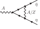
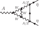
(a)   (b)   (c)

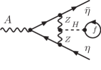
(d)   (e)   (f)

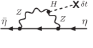
Figure 1: Some higher-order diagrams contributing to the unrenormalized vertex functions $\Gamma^{V\bar{\eta}\eta}_{\mu}$ (graphs a–c) and $\Gamma^{\bar{\eta}\eta}$ (graphs d–f), which receive contributions from 1PI diagrams (graphs a, b, d, e), from explicit tadpole diagrams (graph c), and from diagrams involving tadpole counterterms $\delta t$ (graph f).

For 1PI diagrams it is obvious that at least two couplings to the $\eta$ line exist, for diagrams with tadpole loops or tadpole counterterms the same holds true, because the Higgs field $H$ does not couple to $\eta$. Since both the photon and the Z boson couple to $\eta$ proportional to $Q_{\eta}$, this means that $\Lambda^{V\bar{\eta}\eta}_{\mu}={\cal O}(Q_{\eta}^{2})$. Similarly, all diagrams contributing to the $\eta$ field renormalization constant $Z_{\eta}$ involve at least two couplings of photons or Z bosons to the $\eta$ line, so that $Z_{\eta}=1+{\cal O}(Q_{\eta}^{2})$. Inserting, thus, $\Gamma^{A\bar{\eta}\eta}_{{\mathrm{R}},\mu}$ from (4.4) into condition (4.2) and keeping only terms linear in $Q_{\eta}$ for $Q_{\eta}\to 0$, we get

$$-Q_{\eta}e\,\bar{u}(p)\gamma_{\mu}u(p)={} \left.\bar{u}(p)\,Z_{\eta}\left[Z_{AA}^{1/2}\,\Gamma^{A\bar{\eta}\eta}_{\mu}(0,-p,p)+Z_{ZA}^{1/2}\,\Gamma^{Z\bar{\eta}\eta}_{\mu}(0,-p,p)\right]u(p)\right|_{p^{2}=m_{\eta}^{2}}$$

$$={} -Q_{\eta}e_{0}\left[Z_{AA}^{1/2}+Z_{ZA}^{1/2}\frac{s_{{\mathrm{w}},0}}{c_{{\mathrm{w}},0}}\right]\bar{u}(p)\gamma_{\mu}u(p)\,+\,{\cal O}(Q_{\eta}^{2}).$$ (4.7)

This relation immediately implies

$$e=e_{0}\left[Z_{AA}^{1/2}+Z_{ZA}^{1/2}\frac{s_{{\mathrm{w}},0}}{c_{{\mathrm{w}},0}}\right],$$ (4.8)

which is the desired relation between $e$ and $e_{0}$. Defining the renormalization constant $Z_{e}$ as in (3.6) and $\delta c_{\scriptscriptstyle{\mathrm{W}}}^{2}$ according to

$$c_{{\mathrm{w}},0}^{2}=1-s_{{\mathrm{w}},0}^{2}=c_{\scriptscriptstyle{\mathrm{W}}}^{2}+\delta c_{\scriptscriptstyle{\mathrm{W}}}^{2}=1-s_{\scriptscriptstyle{\mathrm{W}}}^{2}+\delta c_{\scriptscriptstyle{\mathrm{W}}}^{2},$$ (4.9)

we can determine $Z_{e}$ from (4.8),

$$Z_{e}=\left[Z_{AA}^{1/2}+Z_{ZA}^{1/2}\sqrt{\frac{s_{\scriptscriptstyle{\mathrm{W}}}^{2}-\delta c_{\scriptscriptstyle{\mathrm{W}}}^{2}}{c_{\scriptscriptstyle{\mathrm{W}}}^{2}+\delta c_{\scriptscriptstyle{\mathrm{W}}}^{2}}}\right]^{-1}.$$ (4.10)

This is fully equivalent to the result quoted and used in Refs. [28, 24, 25].

5 Generalization to non-standard gauge groups

The concepts of OS renormalization of the photon field, of charge universality, and of charge renormalization as described in the previous sections can be generalized easily to electroweak gauge groups of the type U(1)${}_{Y}{\times}G$, where $G$ is any Lie group of rank $r$ (not necessarily simple or semisimple) and the U(1)_Y group factor plays the analogous role of weak hypercharge in the SM. More precisely, we mean by this that the U(1)_em subgroup of electromagnetic gauge transformations mixes transformations of U(1)_Y and $G$, so that the photon field $A^{\mu}$ is a non-trivial linear combination of the U(1)_Y gauge field $B^{\mu}$ and the gauge fields $C_{k}^{\mu}$ ($k=1,\dots,r$) of $G$ corresponding to the diagonal group generators in the Lie algebra of $G$. The mechanism of electroweak symmetry breaking in the considered gauge theory is widely general, we only assume that electromagnetic gauge invariance is unbroken. Specific types of such models are, for instance, described in Ref. [33] and Ref. [34] with gauge groups U(1)$\times$SU(2)$\times$U(1) and U(1)$\times$SU(3), respectively. If $G$ involves explicit U(1) group factors, the kinetic Lagrangian for the gauge fields in general includes mixing terms $\propto B_{\mu\nu}C_{k}^{\mu\nu}$ with $B^{\mu\nu}$ and $C_{k}^{\mu\nu}$ representing the corresponding (gauge-invariant) U(1) field-strength tensors.

Since the generalization of the previous sections to the considered class of models is straightforward, we can restrict our presentation to the salient steps. We first have to quantify the transformation of the original gauge fields $B^{\mu}$ and $\{C_{k}^{\mu}\}$ to (canonically normalized) fields that correspond to mass eigenstates:

$$\begin{pmatrix}B^{\mu}\\ C_{1}^{\mu}\\ \vdots\\ C_{r}^{\mu}\end{pmatrix}=R\begin{pmatrix}A^{\mu}\\ Z_{1}^{\mu}\\ \vdots\\ Z_{r}^{\mu}\end{pmatrix},\qquad R=\begin{pmatrix}R_{BA}&R_{BZ_{1}}&\cdots&R_{BZ_{r}}\\ R_{C_{1}A}&R_{C_{1}Z_{1}}&\cdots&R_{C_{1}Z_{r}}\\ \vdots&\vdots&\ddots&\vdots\\ R_{C_{r}A}&R_{C_{r}Z_{1}}&\cdots&R_{C_{r}Z_{r}}\end{pmatrix}.$$ (5.1)

Here, the fields $Z_{k}^{\mu}$ ($k=1,\dots,r$) describe neutral massive gauge bosons similar to the Z boson of the SM, and the matrix $R$ is a generalization of the SM rotation matrix parametrized by the weak mixing angle. Note that $R$ is not necessarily orthogonal or unitary, in particular in the presence of kinetic mixing among the original gauge fields.

On-shell renormalization in the photon–Z-boson sector

Marking bare fields and parameters again with suffixes “0”, we parametrize the field renormalization transformation as follows,

$$\begin{pmatrix}A_{0}^{\mu}\\ Z_{0,1}^{\mu}\\ \vdots\\ Z_{0,r}^{\mu}\end{pmatrix}=\begin{pmatrix}Z^{1/2}_{AA}&Z^{1/2}_{AZ_{1}}&\cdots&Z^{1/2}_{AZ_{r}}\\ Z^{1/2}_{Z_{1}A}&Z^{1/2}_{Z_{1}Z_{1}}&\cdots&Z^{1/2}_{Z_{1}Z_{r}}\\ \vdots&\vdots&\ddots&\vdots\\ Z^{1/2}_{Z_{r}A}&Z^{1/2}_{Z_{r}Z_{1}}&\cdots&Z^{1/2}_{Z_{r}Z_{r}}\end{pmatrix}\begin{pmatrix}A^{\mu}\\ Z_{1}^{\mu}\\ \vdots\\ Z_{r}^{\mu}\end{pmatrix},$$ (5.2)

similar to (2.4) in the SM. Making use of the same definitions for vertex functions and self-energies as in Section 2.1, the renormalized transversal parts of the two-point functions of neutral gauge bosons are given by

$$\Gamma^{V^{\prime}V}_{{\mathrm{R}},{\mathrm{T}}}(k^{2})={} -\delta_{V^{\prime}V}\,(k^{2}-\delta_{VZ_{k}}\,M_{{\mathrm{Z}}_{k}}^{2})-\Sigma^{V^{\prime}V}_{{\mathrm{R}},{\mathrm{T}}}(k^{2})$$

$$={} -Z^{1/2}_{AV^{\prime}}Z^{1/2}_{AV}k^{2}-\sum_{k}Z^{1/2}_{Z_{k}V^{\prime}}Z^{1/2}_{Z_{k}V}(k^{2}-M_{{\mathrm{Z}}_{k}}^{2}-\delta M_{{\mathrm{Z}}_{k}}^{2})-\Sigma^{V^{\prime}V}_{{\mathrm{SR}},{\mathrm{T}}}(k^{2}),$$ (5.3)

with $V,V^{\prime}=A,Z_{1},\dots,Z_{r}$. The OS renormalization conditions (2.14) and (2.15) for external photons analogously hold for the $AA$ and all $Z_{k}A$ vertex functions and imply

$$0={} \Gamma^{Z_{k}A}_{{\mathrm{R}},{\mathrm{T}}}(0)=-\Sigma^{Z_{k}A}_{{\mathrm{R}},{\mathrm{T}}}(0)=\sum_{l}Z^{1/2}_{Z_{l}Z_{k}}Z^{1/2}_{Z_{l}A}(M_{{\mathrm{Z}}_{l}}^{2}+\delta M_{{\mathrm{Z}}_{l}}^{2})-\Sigma^{Z_{k}A}_{{\mathrm{SR}},{\mathrm{T}}}(0),$$ (5.4)

$$0={} 1+\Gamma^{AA\,\prime}_{{\mathrm{R}},{\mathrm{T}}}(0)=-\Sigma^{AA\,\prime}_{{\mathrm{R}},{\mathrm{T}}}(0)=1-Z_{AA}-\sum_{k}Z_{Z_{k}A}-\Sigma^{AA\,\prime}_{{\mathrm{SR}},{\mathrm{T}}}(0).$$ (5.5)

Similar to (2.16) and (2.17) in the SM, these conditions can be used to calculate the renormalization constants $Z_{Z_{k}A}$ and $Z_{AA}$ recursively order by order from the relations

$$Z^{1/2}_{Z_{k}A}={} \frac{\Sigma^{Z_{k}A}_{{\mathrm{SR}},{\mathrm{T}}}(0)-\sum_{l\,(l\neq k)}Z^{1/2}_{Z_{l}Z_{k}}Z^{1/2}_{Z_{l}A}(M_{{\mathrm{Z}}_{l}}^{2}+\delta M_{{\mathrm{Z}}_{l}}^{2})}{Z^{1/2}_{Z_{k}Z_{k}}\,(M_{{\mathrm{Z}}_{k}}^{2}+\delta M_{{\mathrm{Z}}_{k}}^{2})},$$ (5.6)

$$Z_{AA}={} 1-\sum_{k}Z_{Z_{k}A}-\Sigma^{AA\,\prime}_{{\mathrm{SR}},{\mathrm{T}}}(0),$$ (5.7)

since the leading behaviour of the occurring renormalization constants is given by

$$Z_{AA}=1+{\cal O}(\alpha),\quad Z^{1/2}_{Z_{k}Z_{l}}=\delta_{kl}+{\cal O}(\alpha),\quad Z^{1/2}_{Z_{k}A}={\cal O}(\alpha),\quad Z^{1/2}_{AZ_{k}}={\cal O}(\alpha),\quad\delta M_{{\mathrm{Z}}_{k}}^{2}={\cal O}(\alpha).$$ (5.8)

For calculating $Z_{Z_{k}A}$ and $Z_{AA}$ at the $n$-loop level, the field renormalization constants $Z^{1/2}_{Z_{k}Z_{l}}$ and the mass renormalization constants $\delta M_{{\mathrm{Z}}_{k}}^{2}$ for the Z_k boson are only required to the $(n-1)$-loop level.

Photon-field renormalization, charge renormalization, and charge universality in the BFM

The invariance of the BFM effective action w.r.t. electromagnetic (background) gauge transformation implies the validity of the Eqs. (2.24)–(2.27) for all $\hat{V}=\hat{A},\hat{Z}_{1},\dots,\hat{Z}_{r}$. Although (2.28) and (2.29) now involve sums of all fields $Z_{k}$, induction in the loop order $n$ can be applied to show

$$Z_{\hat{Z}_{k}\hat{A}}=0,\qquad k=1,\dots,r,$$ (5.9)

and, thus, also

$$Z_{\hat{A}\hat{A}}=1-\Sigma^{\hat{A}\hat{A}\,\prime}_{{\mathrm{SR}},{\mathrm{T}}}(0).$$ (5.10)

With these results, the whole derivation of $Z_{e}$ described in Section 3 for the BFM goes through with the only modification of extending some sums over $\hat{V}=\hat{A},\hat{Z}$ to sums over $\hat{V}=\hat{A},\hat{Z}_{1},\dots,\hat{Z}_{r}$. As a result, the charge renormalization constant $Z_{e}$ is given by $Z_{e}=Z_{\hat{A}\hat{A}}^{-1/2}$ as in (3.13). This again proves charge universality in the model, independent of the use of the BFM in the proof.

Charge universality in $R_{\xi}$-gauge

To exploit charge universality in the determination of $Z_{e}$ in arbitrary $R_{\xi}$-gauge, we again introduce a fake fermion $\eta$ with the same properties as described in Section 4, i.e. $\eta$ only carries infinitesimal hypercharge $Y_{{\mathrm{w}},\eta}$, but no non-trivial quantum number of $G$. If the model contains singlet scalars $S_{i}$, the scalars $S_{i}$ may couple to $\eta$ via Yukawa couplings. The corresponding couplings $y_{i}$ are free parameters of the model and can be taken to be infinitesimally small in analogy to $Q_{\eta}\to 0$, so that decoupling of $\eta$ is guaranteed. The Lagrangian ${\cal L}_{\eta}$, thus, reads

$${\cal L}_{\eta}={} \bar{\eta}\Bigl{(}{\mathrm{i}}\mathchoice{\hbox to0.0pt{\hss$\displaystyle/$\hss\kern-6.97566pt}\hbox{$\displaystyle\partial$}}{\hbox to0.0pt{\hss$\textstyle/$\hss\kern-6.97566pt}\hbox{$\textstyle\partial$}}{\hbox to0.0pt{\hss$\scriptstyle/$\hss\kern-5.38295pt}\hbox{$\scriptstyle\partial$}}{\hbox to0.0pt{\hss$\scriptscriptstyle/$\hss\kern-4.32114pt}\hbox{$\scriptscriptstyle\partial$}}-{\textstyle\frac{1}{2}}g_{1}Y_{{\mathrm{w}},\eta}\mathchoice{\hbox to0.0pt{\hss$\displaystyle/$\hss\kern-8.0868pt}\hbox{$\displaystyle B$}}{\hbox to0.0pt{\hss$\textstyle/$\hss\kern-8.0868pt}\hbox{$\textstyle B$}}{\hbox to0.0pt{\hss$\scriptstyle/$\hss\kern-5.66075pt}\hbox{$\scriptstyle B$}}{\hbox to0.0pt{\hss$\scriptscriptstyle/$\hss\kern-4.0434pt}\hbox{$\scriptscriptstyle B$}}-m_{\eta}-\sum_{i}y_{i}S_{i}\Bigr{)}\eta$$

$$={} \overline{\eta}\bigg{[}{\mathrm{i}}\mathchoice{\hbox to0.0pt{\hss$\displaystyle/$\hss\kern-6.97566pt}\hbox{$\displaystyle\partial$}}{\hbox to0.0pt{\hss$\textstyle/$\hss\kern-6.97566pt}\hbox{$\textstyle\partial$}}{\hbox to0.0pt{\hss$\scriptstyle/$\hss\kern-5.38295pt}\hbox{$\scriptstyle\partial$}}{\hbox to0.0pt{\hss$\scriptscriptstyle/$\hss\kern-4.32114pt}\hbox{$\scriptscriptstyle\partial$}}-Q_{\eta}e\bigg{(}\mathchoice{\hbox to0.0pt{\hss$\displaystyle/$\hss\kern-7.50002pt}\hbox{$\displaystyle A$}}{\hbox to0.0pt{\hss$\textstyle/$\hss\kern-7.50002pt}\hbox{$\textstyle A$}}{\hbox to0.0pt{\hss$\scriptstyle/$\hss\kern-5.25pt}\hbox{$\scriptstyle A$}}{\hbox to0.0pt{\hss$\scriptscriptstyle/$\hss\kern-3.75pt}\hbox{$\scriptscriptstyle A$}}+\sum_{k}\frac{R_{BZ_{k}}}{R_{BA}}\mathchoice{\hbox to0.0pt{\hss$\displaystyle/$\hss\kern-7.54167pt}\hbox{$\displaystyle Z$}}{\hbox to0.0pt{\hss$\textstyle/$\hss\kern-7.54167pt}\hbox{$\textstyle Z$}}{\hbox to0.0pt{\hss$\scriptstyle/$\hss\kern-5.27916pt}\hbox{$\scriptstyle Z$}}{\hbox to0.0pt{\hss$\scriptscriptstyle/$\hss\kern-3.77083pt}\hbox{$\scriptscriptstyle Z$}}_{k}\bigg{)}-m_{\eta}-\sum_{i}y_{i}S_{i}\bigg{]}\eta,$$ (5.11)

where we have identified

$$\textstyle\frac{1}{2}Y_{{\mathrm{w}},\eta}=Q_{\eta},\qquad g_{1}R_{BA}=e.$$ (5.12)

Following the same reasoning as in Section 4, the renormalized $A\bar{\eta}\eta$ vertex function is given by

$$\Gamma^{A\bar{\eta}\eta}_{{\mathrm{R}},\mu}(k,\bar{p},p)=Z_{\eta}Z_{AA}^{1/2}\,\Gamma^{A\bar{\eta}\eta}_{\mu}(k,\bar{p},p)+\sum_{k}Z_{\eta}Z_{Z_{k}A}^{1/2}\,\Gamma^{Z_{k}\bar{\eta}\eta}_{\mu}(k,\bar{p},p),$$ (5.13)

with the unrenormalized $V\bar{\eta}\eta$ vertex functions

$$\Gamma^{A\bar{\eta}\eta}_{\mu}(k,\bar{p},p)={} -Q_{\eta}e_{0}\gamma_{\mu}+e_{0}\Lambda^{A\bar{\eta}\eta}_{\mu}(k,\bar{p},p),$$ (5.14)

$$\Gamma^{Z_{k}\bar{\eta}\eta}_{\mu}(k,\bar{p},p)={} -Q_{\eta}e_{0}\,\frac{R_{0,BZ_{k}}}{R_{0,BA}}\,\gamma_{\mu}+e_{0}\Lambda^{Z_{k}\bar{\eta}\eta}_{\mu}(k,\bar{p},p).$$ (5.15)

Again the vertex corrections $\Lambda^{A\bar{\eta}\eta}_{\mu}$ and $\Lambda^{Z_{k}\bar{\eta}\eta}_{\mu}$ as well as the field renormalization constant $\delta Z_{\eta}=Z_{\eta}-1$ receive only corrections that are suppressed at least by quadratic factors in the new couplings, such as $Q_{\eta}^{2}$ or $Q_{\eta}y_{i}$. Typical diagrams contributing to those corrections at the order ${\cal O}(Q_{\eta}^{2})$ (or higher in $Q_{\eta}$) can be obtained from the graphs shown in Fig. 1 upon interpreting the field $Z$ as any of the $Z_{k}$ and taking the Higgs field $H$ as a any Higgs field of the model. Equation (4) then generalizes to the considered model in an obvious way, and we obtain the final result for the charge renormalization constant:

$$Z_{e}=\left[Z_{AA}^{1/2}+\sum_{k}Z_{Z_{k}A}^{1/2}\,\frac{R_{BZ_{k}}+\delta R_{BZ_{k}}}{R_{BA}+\delta R_{BA}}\right]^{-1}.$$ (5.16)

Here we have formally introduced renormalization constants $\delta R_{BA}$ and $\delta R_{BZ_{k}}$ for the matrix elements of $R$ according to $R_{0}=R+\delta R$, but we have to keep in mind that not all those constants are independent, because not all elements of $R$ are independent free parameters of the theory. Finally, we specialize (5.16) to the one-loop level, which is sufficient for most applications. To this end, we expand the charge and field renormalization constants according to

$$Z_{e}=1+\delta Z_{e}+{\cal O}(\alpha^{2}),\qquad Z_{AA}^{1/2}=1+\textstyle\frac{1}{2}\delta Z_{AA}+{\cal O}(\alpha^{2}),\qquad Z_{Z_{k}A}^{1/2}=\textstyle\frac{1}{2}\delta Z_{Z_{k}A}+{\cal O}(\alpha^{2})$$ (5.17)

and find

$$\delta Z_{e}=-\frac{1}{2}\delta Z_{AA}-\frac{1}{2}\sum_{k}\frac{R_{BZ_{k}}}{R_{BA}}\,\delta Z_{Z_{k}A}.$$ (5.18)

At one loop, $Z_{e}$ is, thus, independent of the renormalization conditions chosen for the mixing matrix $R$ and for the Z-boson masses $M_{{\mathrm{Z}}_{k}}$.

The case of the SM is trivially recovered from the results of this section upon identifying $G={}$SU(2)_w, $r=1$, $Z_{1}^{\mu}=Z^{\mu}$, $R_{BZ_{1}}=s_{\scriptscriptstyle{\mathrm{W}}}$, and $R_{BA}=c_{\scriptscriptstyle{\mathrm{W}}}$.

6 Conclusions

In this article we have derived an all-order form for the renormalization constant $Z_{e}$ of electric charge, as defined in the Thomson limit, in an arbitrary $R_{\xi}$-gauge which expresses $Z_{e}$ in terms of self-energies of the photon–Z-boson system only. We confirm the result that has been given in the literature before, but the derivations of which are either tied to specific gauges, restricted to the two-loop level, or even contain inconsistencies. Our derivation, thus, provides an a posteriori justification for the few calculations of two-loop electroweak corrections based on the assumed form for $Z_{e}$.

Our derivation exploits charge universality, i.e. the fact that the electric unit charge can be defined from the Thomson (low-energy/momentum) limit of the photonic interaction with any charged fermion. Charge universality, for instance, follows from the known universal form of the charge renormalization constant within the background-field formalism, which we have rederived in this paper as well. Exploiting charge universality, we formulate the charge renormalization condition for the photonic interaction of a fake fermion with infinitesimal weak hypercharge and vanishing weak isospin, which effectively decouples from all other particles. Without spelling out the details in this paper, we have repeated the derivation with a fake boson of spin 0 which produces the same universal result for $Z_{e}$ as for the fake fermion. Charge universality, thus, holds for spin-0 bosons too, as expected.

Moreover, we have discussed the derivation of $Z_{e}$ both in the conventional quantization formalism for gauge theories and in the background-field method. Since the determination of $Z_{e}$ in the Thomson limit of the fermion–photon vertex with on-shell fermions and an on-shell photon is based on the property of an S-matrix element, the result on $Z_{e}$ has to be independent of the chosen gauge or quantization procedure. Comparing the explicit results for $Z_{e}$ obtained via different gauges or quantization procedures order by order, therefore provides useful checks on higher-order calculations.

The presented derivation of charge renormalization only makes use of the gauge structure of the model, but does not depend on the matter particle content, the Higgs sector, or other properties. Thus, the result for $Z_{e}$ as obtained for the SM literally holds in all spontaneously broken gauge theories with the SU(2)${}_{\mathrm{w}}\times$U(1)_Y gauge group and SM-like gauge symmetry breaking in the electroweak sector. Finally, we have determined the charge renormalization constant to all perturbative orders in the more general class of spontaneously broken gauge theories with gauge group U(1)${}_{Y}{\times}G$ with any Lie group $G$, only assuming that electromagnetic gauge symmetry is unbroken and mixes with U(1)_Y transformations in a non-trivial way.

Appendix

Problems in previous all-order determinations of $Z_{e}$

In Ref. [28], the derivation of the charge renormalization constant $Z_{e}$ starts from the ST identity obtained from the vanishing BRS variation of the Green function $\langle 0|T\,\bar{u}^{A}(x)\,\psi_{f}(y)\,\bar{\psi}_{f}(z)\,|0\rangle$. Translating the corresponding relations in Sects. 4.2 and 4.3 of Ref. [28] to the conventions of Ref. [14], this schematically implies

$$0={} k^{\mu}G_{\mu}^{Af\bar{f}}(k,p_{1},p_{2})+a_{Z}k^{\mu}G_{\mu}^{Zf\bar{f}}(k,p_{1},p_{2})+a_{\chi}G^{\chi f\bar{f}}(k,p_{1},p_{2})$$

$${}+\sum_{V=A,Z}a^{Y}_{fV}\int\frac{{\mathrm{d}}^{D}q}{(2\pi)^{D}}\left[G^{u^{V}\bar{u}^{A}f^{\prime}\bar{f}}(q,k,p_{1}-q,p_{2})-G^{u^{V^{\dagger}}\bar{u}^{A}f\bar{f}^{\prime}}(q,k,p_{1},p_{2}-q)\right]$$

$${}+\sum_{V=Z,W^{\pm}}a^{\mathrm{w}}_{fV}\int\frac{{\mathrm{d}}^{D}q}{(2\pi)^{D}}\left[\omega_{-}G^{u^{V}\bar{u}^{A}f^{\prime}\bar{f}}(q,k,p_{1}-q,p_{2})-G^{u^{V^{\dagger}}\bar{u}^{A}f\bar{f}^{\prime}}(q,k,p_{1},p_{2}-q)\omega_{+}\right],$$ (A.1)

where the constants $a_{Z}$, $a_{\chi}$ are determined by the gauge-fixing term of the photon field. The constants $a^{Y}_{fV}$ and $a^{\mathrm{w}}_{fV}$ express the transformation properties of the fermion $f$ w.r.t. U(1)_Y and SU(2)_w gauge transformations, respectively. In case $V$ is a charged gauge boson, the field $f^{\prime}$ is the field of its weak isospin partner, otherwise $f^{\prime}=f$. Figure 2 illustrates some Feynman diagrams and diagram types contributing to the Green functions $G^{u^{V}\bar{u}^{A}f^{\prime}\bar{f}}$; graphs contributing to $G^{u^{V^{\dagger}}\bar{u}^{A}f\bar{f}^{\prime}}$ look similar, with the ghost and fermion lines meeting in the field point at $z$.

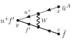
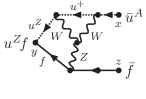
(a)   (b)   (c)

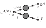
Figure 2: Various graphs contributing to the $\int{\mathrm{d}}^{D}q\,G^{u^{V}\bar{u}^{A}f^{\prime}\bar{f}}(q,k,p_{1}-q,p_{2})$ in momentum space, which correspond to the Green functions $G^{u^{V}\bar{u}^{A}f^{\prime}\bar{f}}(y,x,y,z)$ in position space: (a,b) two connected graphs and (c) the generic graph for disconnected parts, with the grey blob representing 1PI or tadpole contributions.

Identity (A.1) is correct and certainly bears the desired information on the Thomson limit of the $Af\bar{f}$ vertex, however, the reasoning explained in Ref. [28] does not hold:

• In order to get rid of the contribution of SU(2)_w gauge bosons in the last line of (A.1), the identity is formulated for right-handed fields, and the mixing between right- and left-handed fields is ignored during the amputation of the external propagators and the projection to on-shell states. This simplification, though, could be dropped by a projection of (A.1) to right-handed chirality from the left and from the right with a subsequent amputation of the full fermion propagators. We have carried out this more laborious procedure at one loop. The oversimplification seems to be no show stopper.

• A serious problem, however, concerns the simultaneous on-shell limit $k\to 0$, $p_{1}^{2}\to m_{f}^{2}$, and $p_{2}^{2}\to m_{f}^{2}$ after amputation, which is presented in Ref. [28] in a sketchy way. The claim that all connected parts of $G^{u^{V}\bar{u}^{A}f^{\prime}\bar{f}}$ and $G^{u^{V^{\dagger}}\bar{u}^{A}f\bar{f}^{\prime}}$ vanish in this limit, unfortunately does not hold, because this multiple limit is more subtle.

  If we first go on shell with the fermion momenta $p_{1}$, $p_{2}$ after amputation, leaving $k$ open, in fact the unpleasant connected parts of $G^{u^{V}\bar{u}^{A}f^{\prime}\bar{f}}$ and $G^{u^{V^{\dagger}}\bar{u}^{A}f\bar{f}^{\prime}}$ vanish due to a missing pole in one of the external fermion legs. The projection of (A.1) to on-shell fermion states leads to a relation between the axial-vector and scalar formfactors of the $Af\bar{f}$ vertex and self-energies for arbitrary $k^{2}$. At one loop we have checked this identity by explicit calculation. For $k^{2}=0$, this identity was, e.g., given as Eq. (3.33) in Ref. [12], as Eq. (3.30) in Ref. [13], or as the second relation in Eq. (C.31) of Ref. [14].

  However, in order to obtain the required relation for the vector formfactor of the $Af\bar{f}$ vertex, which is, e.g., given as Eq. (3.27) in Ref. [12], as Eq. (3.29) in Ref. [13], or as the first relation in Eq. (C.31) of Ref. [14] at one loop, the on-shell limit has to be carried out differently: Only one of the fermion momenta, called $p$ in the following, can be set on shell at the beginning, followed by an derivative w.r.t. the photon momentum $k$, with subsequently taking $k\to 0$. With the last step, the second fermion line goes on shell automatically. Note that taking the derivative w.r.t. $k$ while keeping $p$ fixed increases the order of the pole in the propagator of the off-shell fermion, which has momentum $p+k$. For $k\to 0$, there are, thus, poles of order two at $p^{2}=m_{f}^{2}$ which prevents the connected parts of $G^{u^{V}\bar{u}^{A}f^{\prime}\bar{f}}$ and $G^{u^{V^{\dagger}}\bar{u}^{A}f\bar{f}^{\prime}}$ from vanishing in the on-shell projection of the two external fermion lines in general.

  At one loop, however, the mentioned terms still vanish if the fermion line is projected to right-handed chirality on both fermion legs, because then no one-loop Feynman diagram exists that links the photonic ghost line to the fermion lines. Beyond one loop, connected graphs contributing $G^{u^{V}\bar{u}^{A}f^{\prime}\bar{f}}$ and $G^{u^{V^{\dagger}}\bar{u}^{A}f\bar{f}^{\prime}}$ exist (see Fig. 2b), and there is no reason for them to vanish.

• Finally, the evaluation of the ghost propagators and their renormalization in the disconnected contributions to $G^{u^{V}\bar{u}^{A}f^{\prime}\bar{f}}$ and $G^{u^{V^{\dagger}}\bar{u}^{A}f\bar{f}^{\prime}}$ in Ref. [28] is not correct. Equations (4.38) and (4.39) of Ref. [28] express the required residues of the $G^{u^{A}\bar{u}^{A}}$ and $G^{u^{Z}\bar{u}^{A}}$ propagators at $k^{2}=0$ in terms of the field renormalization constants $Z_{AA}$ and $Z_{ZA}$, respectively. However, since $Z_{AA}$ already involves non-vanishing contributions from closed fermion loops, but $G^{u^{A}\bar{u}^{A}}$ does not, Eq. (4.38) of Ref. [28] is obviously invalid.

  The correct evaluation of the ghost propagators can, e.g., be based on the BRS invariance of the (unrenormalized) Green function $\langle|T\,\bar{u}^{A}(x)\,B^{\mu}(y)\,|0\rangle$. The resulting ST identity for the ghost propagators expresses $G^{u^{B}\bar{u}^{A}}$ in terms of the longitudinal part of the $AZ$ self-energy.

With the help of the mentioned corrections,we have successfully derived the known form of $Z_{e}$ at the one-loop level, starting from the ST identity (A.1), which provides an alternative to the derivation described in App. C of Ref. [14] based on Lee identities. We do, however, not see a way how to carry out a corresponding all-order proof by simple amendments.

Completely independent of the proof based on (A.1), it was suggested in Ref. [28] and in App. A of Ref. [25] to deduce $Z_{e}$ from the fact that the product $g_{1}B^{\mu}$ need not be renormalized. This fact is justified in those papers upon referring to Sect. 3.4.3 of Ref. [10] where it was deduced from Lee identities in the course of proving charge universality. Since this derivation in Ref. [10] is carried out in the Landau gauge, it is actually not clear without further justification that no modifications are necessary in general $R_{\xi}$-gauge. At the two-loop level, this missing justification was provided in Refs. [29, 30, 31] where the non-renormalizability of $g_{1}B^{\mu}$ was first assumed for charge renormalization and in a second step checked by explicit calculation that all $Af\bar{f}$ vertex corrections vanish in the Thomson limit. A corresponding all-order proof that the non-renormalizability hypothesis of $g_{1}B^{\mu}$ is equivalent to charge renormalization in the Thomson limit in arbitrary $R_{\xi}$-gauge to all orders, to our knowledge, does not exist in the literature.

References

- [1] W. E. Thirring, Radiative corrections in the nonrelativistic limit, Phil. Mag. Ser. 7 41 (1950) 1193–1194.
- [2] M. E. Peskin and D. V. Schroeder, An introduction to quantum field theory. Addison-Wesley, Reading, USA, 1995.
- [3] S. Weinberg, The quantum theory of fields. Vol. 2: Modern applications. Cambridge University Press, Cambridge, UK, 2013.
- [4] M. Böhm, A. Denner, and H. Joos, Gauge theories of the strong and electroweak interaction. Teubner, Stuttgart, Germany, 2001.
- [5] M. D. Schwartz, Quantum Field Theory and the Standard Model. Cambridge University Press, Cambridge, UK, 2014.
- [6] D. A. Ross and J. C. Taylor, Renormalization of a unified theory of weak and electromagnetic interactions, Nucl. Phys. B51 (1973) 125–144. [Erratum: Nucl. Phys. B58 (1973) 643].
- [7] A. Sirlin, Radiative Corrections in the Theory: A Simple Renormalization Framework, Phys. Rev. D22 (1980) 971–981.
- [8] D. Yu. Bardin, P. K. Khristova, and O. M. Fedorenko, On the lowest order electroweak corrections to spin 1/2 fermion scattering. (I). The one-loop diagrammar, Nucl. Phys. B175 (1980) 435–461.
- [9] J. Fleischer and F. Jegerlehner, Radiative corrections to Higgs-boson decays in the Weinberg-Salam Model, Phys. Rev. D23 (1981) 2001–2026.
- [10] K.-i. Aoki, Z. Hioki, M. Konuma, R. Kawabe, and T. Muta, Electroweak Theory: Framework of On-Shell Renormalization and Study of Higher Order Effects, Prog. Theor. Phys. Suppl. 73 (1982) 1–225.
- [11] M. Böhm, H. Spiesberger, and W. Hollik, On the 1-Loop Renormalization of the Electroweak Standard Model and its Application to Leptonic Processes, Fortsch. Phys. 34 (1986) 687–751.
- [12] W. F. L. Hollik, Radiative Corrections in the Standard Model and their Role for Precision Tests of the Electroweak Theory, Fortsch. Phys. 38 (1990) 165–260.
- [13] A. Denner, Techniques for the Calculation of Electroweak Radiative Corrections at the One-Loop Level and Results for W-physics at LEP200, Fortsch. Phys. 41 (1993) 307–420, [arXiv:0709.1075].
- [14] A. Denner and S. Dittmaier, Electroweak Radiative Corrections for Collider Physics, Phys. Rept. 864 (2020) 1–163, [arXiv:1912.0682].
- [15] A. Denner, G. Weiglein, and S. Dittmaier, Application of the Background Field Method to the electroweak Standard Model, Nucl. Phys. B440 (1995) 95–128, [hep-ph/9410338].
- [16] B. S. DeWitt, Quantum Theory of Gravity. 2. The Manifestly Covariant Theory, Phys. Rev. 162 (1967) 1195–1239.
- [17] G. ’t Hooft, The Background Field Method in Gauge Field Theories, in Functional and Probabilistic Methods in Quantum Field Theory. Proceedings, 12th Winter School of Theoretical Physics, Karpacz, Feb 17-March 2, 1975, pp. 345–369, 1975.
- [18] B. S. DeWitt, A gauge invariant effective action, in Oxford Conference on Quantum Gravity Oxford, England, April 15-19, 1980, pp. 449–487, 1980.
- [19] D. G. Boulware, Gauge Dependence of the Effective Action, Phys. Rev. D23 (1981) 389.
- [20] L. F. Abbott, The Background Field Method Beyond One Loop, Nucl. Phys. B185 (1981) 189–203.
- [21] L. F. Abbott, Introduction to the Background Field Method, Acta Phys. Polon. B13 (1982) 33.
- [22] S. Dittmaier, Thirring’s low-energy theorem and its generalizations in the electroweak Standard Model, Phys. Lett. B409 (1997) 509–516, [hep-ph/9704368].
- [23] G. Degrassi and A. Vicini, Two loop renormalization of the electric charge in the standard model, Phys. Rev. D 69 (2004) 073007, [hep-ph/0307122].
- [24] A. Freitas, W. Hollik, W. Walter, and G. Weiglein, Electroweak two-loop corrections to the – mass correlation in the Standard Model, Nucl. Phys. B632 (2002) 189–218, [hep-ph/0202131]. [Erratum: Nucl. Phys. B666 (2003) 305].
- [25] M. Awramik, M. Czakon, A. Onishchenko, and O. Veretin, Bosonic corrections to at the two-loop level, Phys. Rev. D68 (2003) 053004, [hep-ph/0209084].
- [26] A. Freitas, Two-loop fermionic electroweak corrections to the Z-boson width and production rate, Phys. Lett. B 730 (2014) 50–52, [arXiv:1310.2256].
- [27] L. Chen and A. Freitas, Mixed EW-QCD leading fermionic three-loop corrections at to electroweak precision observables, arXiv:2012.0860.
- [28] S. Bauberger, Two-loop contributions to muon decay. PhD thesis, Würzburg U., 1997.
- [29] S. Actis, A. Ferroglia, M. Passera, and G. Passarino, Two-Loop Renormalization in the Standard Model. Part I: Prolegomena, Nucl. Phys. B777 (2007) 1–34, [hep-ph/0612122].
- [30] S. Actis and G. Passarino, Two-Loop Renormalization in the Standard Model Part II: Renormalization Procedures and Computational Techniques, Nucl. Phys. B777 (2007) 35–99, [hep-ph/0612123].
- [31] S. Actis and G. Passarino, Two-Loop Renormalization in the Standard Model Part III: Renormalization Equations and their Solutions, Nucl. Phys. B777 (2007) 100–156, [hep-ph/0612124].
- [32] A. Denner, S. Dittmaier, and J.-N. Lang, Renormalization of mixing angles, JHEP 11 (2018) 104, [arXiv:1808.0346].
- [33] K. Babu, C. F. Kolda, and J. March-Russell, Implications of generalized Z - Z-prime mixing, Phys. Rev. D 57 (1998) 6788–6792, [hep-ph/9710441].
- [34] F. Pisano and V. Pleitez, An SU(3) x U(1) model for electroweak interactions, Phys. Rev. D 46 (1992) 410–417, [hep-ph/9206242].