Two-loop renormalization of the electric charge
in the Standard Model

Abstract

We discuss the renormalization of the electric charge at the two-loop level in the Standard Model of the electroweak interactions. We explicitly calculate the expression of the complete on-shell two-loop counterterm using the Background Field Method and discuss the advantages of this computational approach. We consider the related quantity $\mbox{$\hat{e}^{2}$}(\mu)$, defined in the $\overline{MS}$ renormalization scheme and present numerical results for different values of the scale $\mu$. We find that the full 2-loop electroweak corrections contribute more than 10 parts in units $10^{-5}$ to the $\Delta\mbox{$\hat{\alpha}$}(m_{\scriptscriptstyle Z}^{2})$ parameter, obtaining $\mbox{$\hat{\alpha}$}^{-1}(m_{\scriptscriptstyle Z})=128.12\pm 0.05$ for $\Delta\alpha^{(5)}_{\rm had}(m_{\scriptscriptstyle Z}^{2})=0.027572\pm 0.000359$.

1 Introduction

The very high experimental precision reached at LEP and prospected at TESLA with the GigaZ option, requires a corresponding theoretical effort to provide accurate predictions. Inclusion of higher order effects and a very precise knowledge of the input parameters of the electroweak Standard Model (SM) are necessary ingredients of precision physics. Among the three basic input parameters usually employed, namely $\alpha,\,G_{\mu}$ and $m_{\scriptscriptstyle Z}$, the fine structure constant defined at zero momentum transfer, $\alpha(0)$, is the most precise one with a relative error of 3.7 parts per billion. However, for physics at high momentum transfer, like physics at the $Z$-resonance, the use of an effective coupling defined at the relevant scale is more appropriate, e.g. for the $Z$-resonance $\alpha(m_{\scriptscriptstyle Z})$ is more adequate than $\alpha(0)$.

In pure QED the natural definition of an effective QED coupling at the scale $\sqrt{s}$

$$\alpha(s) = \frac{\alpha}{1-\Delta\alpha(s)}$$ (1)

$$\Delta\alpha(s) = 4\pi\alpha\,{\rm Re}\,\left[\Pi_{\gamma\gamma}(s)-\Pi_{\gamma\gamma}(0)\right]~{},$$ (2)

is given in terms of the photon vacuum polarization function evaluated at different scales.

In the full SM, the bosonic contribution to the photon vacuum polarization at high momentum transfer is, in general, not gauge-invariant. Thus it cannot be included in a sensible way in Eq.(1). Eq.(1) with only the fermionic contribution included is a good effective coupling at the $m_{\scriptscriptstyle Z}$ scale. However, for energy scales much higher than $m_{\scriptscriptstyle Z}$, that will be tested by the future accelerators, an effective QED coupling that takes into account also the bosonic contributions can be considered.

A different definition of a QED effective coupling can be obtained by considering the $\overline{MS}$ QED coupling constant at the scale $\mu$ defined by

$$\mbox{$\hat{\alpha}$}(\mu)=\frac{\alpha}{1+(2\hat{\delta e}/e)}~{}.$$ (3)

Eq.(3) is expressed in terms of the finite part of the on-shell electric charge counterterm (i.e. with the dimensional regularization pole subtracted), which is gauge-invariant quantity that includes both fermionic and bosonic contributions. In the Background Field Method (BFM), as it will be discussed in detail in section 3, the counterterm is given only by the photon vacuum polarization diagrams, evaluated at $q^{2}=0$. At the one-loop level the electric charge renormalization has been discussed in [1, 2].

In this paper we present explicit results for the electric charge counterterm including all second order ${\cal O}(\alpha^{2})$ electroweak corrections. Our calculation is performed employing the BFM framework. The issue of the two-loop renormalization of the electric charge in the SM was already addressed in the usual $R_{\xi}$ gauge quantization scheme by several papers discussing the two-loop contributions to the $m_{\scriptscriptstyle W}$-$m_{\scriptscriptstyle Z}$ interdependence [3]. Our calculation provides the necessary ingredients to define and evaluate numerically the effective parameter $\mbox{$\hat{e}^{2}$}(\mu)$, which is a fundamental quantity in all precision tests of the SM.

The paper is structured in the following way. In Section 2 we outline the calculation of the Thomson scattering amplitude, which allows to define the electric charge counterterm, and present the 1-loop result in the SM. In Section 3 we discuss the main differences between the usual $R_{\xi}$ gauge quantization scheme and the approach offered by the BFM, that makes manifest the possibility of a Dyson summation also for the bosonic contribution. In Section 4 we present the results of our calculation of the Thomson scattering amplitude at the 2-loop level and comment on the checks that we made. In Section 5 we discuss in detail the $\overline{MS}$ parameter $\mbox{$\hat{e}^{2}$}(\mu)$, present numerical results for this parameter for different values of the scale $\mu$, and discuss the relevance at $\mu=m_{\scriptscriptstyle Z}$ of the contributions we have computed. Finally, we comment on the variation of the 95 % upper limit on the Higgs boson mass induced by our new result on $\mbox{$\hat{\alpha}$}(m_{\scriptscriptstyle Z})$.

2 Structure of the calculation

The electric charge is defined in terms of Thomson scattering, namely of the scattering of a fermion off a photon of vanishingly small energy. The diagrams that describe this process in the SM can be depicted symbolically as in fig. 1.

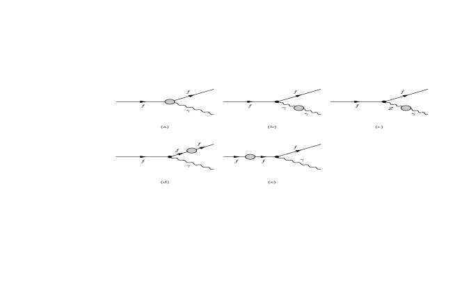
Figure 1: The diagrams of the Thomson scattering

As it is well known in pure QED the $\gamma$–$Z$ mixing diagram (1c) is absent while the Ward–Takahashi identity ensures the cancellation of the vertex contribution (1a) against the wave function renormalization of the fermion (1d, 1e) such that the relation between the bare charge $e_{0}$ and the conventional renormalized charge $e$ can be written, via Dyson summation, as:

$$e^{2}={e^{2}_{0}\over 1-e^{2}_{0}\,\mbox{$\Pi^{\mbox{\scriptsize{(f)}}}_{\gamma\gamma}$}(0)}$$ (4)

where $\mbox{$\Pi^{\mbox{\scriptsize{(f)}}}_{\gamma\gamma}$}(0)$ is the fermionic QED vacuum-polarization function evaluated at $q^{2}=0$.

We write in general a vector boson (V) self-energy as

$$\Pi^{\mu\nu}_{VV}(q^{2})=A_{VV}(q^{2})g^{\mu\nu}+B_{VV}(q^{2})q^{\mu}q^{\nu},$$ (5)

employing the convention that the photon vacuum polarization function is related to the transverse part of its self-energy by

$$A_{\gamma\gamma}(q^{2})=q^{2}\,e^{2}_{0}\,\Pi_{\gamma\gamma}(q^{2})~{}.$$ (6)

The discussion of the Thomson scattering in the full SM when the theory is quantized employing the conventional linear $R_{\xi}$ gauge-fixing procedure [4] differs from the QED case. We recall that in the $R_{\xi}$ gauges the classical Lagrangian is supplemented by a gauge fixing function of the form

$${\cal L}^{g.f.}_{R_{\xi}} = -\frac{1}{2\xi}\left(F_{\gamma}^{2}+F_{Z}^{2}+2F_{+}F_{-}\right)$$ (7)

$$F_{\pm} = \partial^{\mu}W^{\pm}_{\mu}\mp i\,\xi\,m_{\scriptscriptstyle W}\phi^{\pm}$$

$$F_{Z} = \partial^{\mu}Z_{\mu}-\xi\,m_{\scriptscriptstyle Z}\chi$$

$$F_{\gamma} = \partial^{\mu}A_{\mu}$$

that cancels, at the tree-level, the mixing between the vector and scalar fields. In Eq.(7) $\phi$ and $\chi$ are the unphysical counterparts associated to the $W$ and $Z$ bosons.

In the SM the radiating fermion couples both to the photon and the $Z$ currents ($J_{\gamma}^{\mu},J_{Z}^{\mu}$), the latter via the $\gamma$–$Z$ mixing diagram, fig.(1c). Furthermore, the theory does not satisfy a QED-like Ward identity, namely the sum of diagrams (1a, 1d, 1e) does not add anymore to zero. Instead they come out proportional to the third current of the weak isospin $J_{3}^{\mu}\equiv 2(J_{Z}^{\mu}+s^{2}J_{\gamma}^{\mu})$ with $s^{2}\equiv\sin^{2}\theta_{W}$, so that the part of $J_{3}^{\mu}$ proportional to the $Z$ current cancels the contribution coming from the $\gamma$–$Z$ mixing in order to obtain a result only proportional to the photonic current. The final result is constituted by the total photon self-energy contribution (fermionic plus bosonic) plus the vertex part from diagrams (1a, 1d, 1e) proportional to $J_{\gamma}^{\mu}$. At the one loop level we have [1]

$$e^{2}=e^{2}_{0}\left\{1+e^{2}_{0}\,\mbox{$\Pi^{\mbox{\scriptsize{(f)}}}_{\gamma\gamma}$}(0)-\frac{7e^{2}_{0}}{8\pi^{2}}\left[\frac{1}{n-4}+\ln\frac{m_{\scriptscriptstyle W}}{\mu}-\frac{1}{21}\right]\right\}\\ \equiv e_{0}^{2}\left(1+\frac{2\delta e^{(1)}}{e}\right),$$ (8)

where $\delta e^{(1)}$ is the on-shell one-loop electric charge counterterm. In Eq.(8) the last term in the curly bracket represents ${\cal O}\!\left(e^{2}_{0}\right)$ bosonic contributions to the charge renormalization and in the $\xi=1$ Feynman gauge 3 out of the 7 parts come from the bosonic contribution to the photon self-energy while the remaining 4 are from the vertex diagrams. In Eq.(8) $n$ is the dimension of the space-time and and $\mu$ is a rescaled ‘t Hooft mass according to

$$\mu\rightarrow{\mu\,e^{\gamma/2}\over(4\pi)^{1/2}}.$$ (9)

The factor $e^{\gamma/2}(4\pi)^{-1/2}$ is appended to the usual ‘t Hooft mass in order to cancel some numerical constants that are an artifact of dimensional regularization [5]. We notice that, because of the presence of non-vanishing vertex contribution, the possibility of a Dyson summation like Eq.(4) in the SM with linear gauge fixing is not manifestly evident.

In general the renormalization of the electric charge in the SM with linear gauge-fixing requires the evaluation of the full set of diagrams of fig. 1 and beyond one-loop level it can become quite complicated although the analysis could be somewhat simplified with an appropriate use of the relevant Ward identity (see section 4). However, the problem cannot be reduced to the calculation of just the photon vacuum polarization as in pure QED because of the lack of a QED-like Ward identity.

3 Background-field method analysis

As it is well known, in a gauge theory the choice of a gauge in order to quantize the theory can spoil in the intermediate steps the original gauge symmetry of the lagrangian that is actually restored at the end when physical processes are considered. This is what actually happens when the SM is quantized with the linear gauge-fixing function of Eq.(7). The BFM [6, 7] is a technique for quantizing gauge theories that avoids the complete explicit breaking of the gauge symmetry. One of the salient features of this approach is that all fields are splitted in two components: a classical background field $\hat{V}$ and a quantum field $V$ that appears only in the loops. The gauge-fixing procedure is achieved through a non linear term in the fields that breaks the gauge invariance only of the quantum part of the lagrangian, preserving the gauge symmetry of the effective action with respect to the background fields. As a result the background field Green functions satisfy simple QED-like Ward identities.

The application of the BFM to the SM was discussed in Ref.[8]. A suitable generalization of the gauge-fixing term of Eq.(7) to the BFM that retains the gauge invariance of the action under background field transformation can be written as [9]:

$${\cal L}^{g.f.}_{BFM} = -\frac{1}{2\xi_{Q}}\left(G_{\gamma}^{2}+G_{Z}^{2}+2G_{+}G_{-}\right)$$ (10)

$$G_{\pm} = \partial^{\mu}W_{\mu}^{\pm}\mp i\,\xi_{Q}\,m_{\scriptscriptstyle W}\phi^{\pm}\pm i\left(e{\hat{A}}_{\mu}-g\,c{\hat{Z}}_{\mu}\right)W_{\mu}^{\pm}\pm i\left(eA_{\mu}-g\,cZ_{\mu}\right){\hat{W}}_{\mu}^{\pm}\mp$$

$$~{}\mp\frac{i}{2}g\xi_{Q}\left[({\hat{H}}\mp i{\hat{\chi}})\phi^{\pm}-(H\mp i\chi){\hat{\phi}}^{\pm}\right]$$

$$G_{Z} = \partial^{\mu}Z_{\mu}-\xi_{Q}\,m_{\scriptscriptstyle Z}\chi+i\,g\,c\left({\hat{W}}_{\mu}^{+}W^{-\mu}-W_{\mu}^{+}{\hat{W}}^{-\mu}\right)+ig\xi_{Q}\frac{c^{2}-s^{2}}{2c\,s}\left({\hat{\phi}}^{+}\phi^{-}-\phi^{+}{\hat{\phi}}^{-}\right)~{}+$$

$$~{}+~{}~{}g\xi_{Q}\frac{1}{2c}\left({\hat{\chi}}H-{\hat{H}}\chi-v\chi\right)$$

$$G_{\gamma} = \partial^{\mu}A_{\mu}+ie\left({\hat{W}}_{\mu}^{+}W^{-\mu}-W_{\mu}^{+}{\hat{W}}^{-\mu}\right)+ie\xi_{Q}\left({\hat{\phi}}^{+}\phi^{-}-\phi^{+}{\hat{\phi}}^{-}\right)$$

where $g$ is the $SU(2)$ coupling, $c\equiv\cos\theta_{W}$, $\xi_{Q}$ the quantum gauge parameter and $H$ the physical Higgs field.

The invariance of the effective action under the relevant background gauge transformation of the background fields allows to write identities that have a simpler structure of the conventional Slavnov-Taylor identities and in general do not involve ghost fields. In particular, for the two and three point functions involving the photon the following identities hold to all orders in perturbation theory.

$$q^{\mu}\Gamma^{\gamma{\bar{f}}f}_{\mu}(q,{\bar{p}},p) = -eQ_{f}\left[\Sigma_{f}({\bar{p}})-\Sigma_{f}(-p)\right]$$ (11)

$$B_{\gamma\gamma}(0) = 0$$ (12)

$$B_{\gamma Z}(0) = 0$$ (13)

where $\Gamma^{\gamma{\bar{f}}f}_{\mu}$ is the three-point function photon-fermion-antifermion, $\Sigma_{f}$ is the fermion two-point function, $q={\bar{p}}+p$ the photon momentum and $Q_{f}$ is the charge of the fermion $f$ in units $e$. Eq.(11) is the usual QED Ward identity. Eqs.(11) and (13) are not true in the conventional $R_{\xi}$ gauges, whilst Eq.(12) is valid at 1-loop but is spoiled by higher order corrections. From Eq.(12) and Eq.(13) and from the analyticity properties of the two-point functions, it follows that, to all orders,

$$A_{\gamma\gamma}(0) = 0$$ (14)

$$A_{\gamma Z}(0) = 0~{}.$$ (15)

In the $R_{\xi}$ gauges Eq.(14) is valid at 1-loop, while Eq.(15) does not hold. An important consequence of Eqs.(11-15) is that in the SM, when the BFM is employed, the renormalization of the electric charge receives contributions only from the photon vacuum polarization, analogously to QED. It follows that the relation between bare charge and the renormalized one can be written as in Eq.(4) and the Dyson summation is justified not only for the QED part but for the complete SM contribution. Therefore in the SM the relation between $e_{0}$ and $e$ is obtained from Eq.(4) with $\mbox{$\Pi^{\mbox{\scriptsize{(f)}}}_{\gamma\gamma}$}(0)$ replaced by the complete (bosonic plus fermionic) $\Pi_{\gamma\gamma}(0)$ evaluated with the BFM Feynman rules for the SM. We would like to stress that, differently from the conventional analysis in the standard $R_{\xi}$ gauge, the BFM approach makes manifest the possibility of the Dyson summation also for the bosonic part of the vacuum polarization function, a fact already discussed in Refs[8, 10].

4 Results

Before presenting the result for the two-loop contribution to the vacuum polarization function we briefly discuss some interesting aspects of a two-loop BFM calculation.

The presence of two different kinds of fields, the background and the quantum ones, requires the introduction of two different sets of Feynman rules, one for the quantum fields that are actually identical to conventional ones, and one for vertices where at least one background field is present. Since the gauge-fixing term of Eq.(10) differs from the conventional one, Eq.(7), by terms that involve both classical and quantum fields, the corresponding mixed vertices are modified. In particular, because Eq.(10) is quadratic in the quantum fields, only vertices in which two quantum fields are present can differ from the conventional ones, like for example the ${\hat{\gamma}}W^{+}W^{-}$ vertex that acquires a $\xi_{Q}$ dependence. Furthermore, the non linearity of the gauge-fixing function induces a modified ghost sector with respect to the linear $R_{\xi}$ gauges. In a two-loop calculation both sets of Feynman rules are needed. In fact, in the case of the electric charge, the external photon is a background field and couples to the bosonic particles running into the loop differently from an internal photon, which instead should be regarded as a quantum field. A complete set of BFM Feynman rules can be found in Ref. [8].

The QED-like BFM identities simplify considerably the renormalization procedure. Indeed, it is convenient to choose a renormalization prescription that automatically respects Eqs.(11-15) and for our two-loop calculation this should be enforced at the one-loop level. Possible subtleties of this implementation are only related to the bosonic sector. We recall that in the one-loop diagrams, besides the fermions for which we employ the usual on-shell mass renormalization, the particles that contribute to the bosonic part of the vacuum polarization, $\mbox{$\Pi^{\mbox{\scriptsize{(b)}}}_{\gamma\gamma}$}(0)$, are the $W$ boson, its unphysical counterpart, and the charged ghosts, whose masses squared are $m_{\scriptscriptstyle W}^{2}$ and $\xi_{Q}m_{\scriptscriptstyle W}^{2}$ respectively. It is then clear that if we renormalize the masses of all these particles in the same way, namely employing the same $W$ mass counterterm, $\delta m_{\scriptscriptstyle W}^{2}$, for all, Eqs.(11-15), that are satisfied at one-loop, will be automatically preserved under renormalization. This choice corresponds to employing a gauge fixing function written in terms of bare parameters and fields. The tadpole contribution needs a detailed comment. We perform the standard tadpole subtraction, namely we choose the tadpole counterterm to cancel the complete one-loop tadpole contribution. This induces an additional term in the mass counterterm of the unphysical scalar proportional to one-loop tadpoles. This contribution is needed to restore a topology of two-loop diagrams canceled by our choice of the tadpole counterterm and does not invalidate the preservation of the QED-like Ward identity under our renormalization prescription.

Several other prescriptions for the renormalization of the gauge fixing part and associated ghost sector are conceivable. In particular, one can add the gauge-fixing term to the renormalized Lagrangian, so that Eq.(10) is expressed in terms of renormalized quantities. In this case, while the mass of unphysical scalar is not renormalized, a part from the tadpole contribution, the counterterm of the charged ghost mass becomes 1/2 that of $W$ boson. However, besides a counterterm for the $W$–$\phi$ transition, several new contributions involving coupling and mass counterterms are induced due to the mismatch between the bare quantities appearing in the classical lagrangian and the renormalized quantities in the gauge-fixing term. We have explicitly verified that the two procedures give the same result. Furthermore we have also explicitly verified the two identities, Eq.(11) and Eq.(15), at the two-loop level in the BFM Feynman gauge, $\xi_{Q}=1$.

The BFM allows to write the relation between the bare and renormalized electric charge as:

$$e^{2} = {e^{2}_{0}\over 1-e^{2}_{0}\,\Pi_{\gamma\gamma}(0)}~{},$$ (16)

$$\Pi_{\gamma\gamma}(0) = \mbox{$\Pi^{\mbox{\scriptsize{(f)}}}_{\gamma\gamma}$}(0)+\mbox{$\Pi^{\mbox{\scriptsize{(b)}}}_{\gamma\gamma}$}(0)~{},$$ (17)

$$\mbox{$\Pi^{\mbox{\scriptsize{(f)}}}_{\gamma\gamma}$}(0) = \mbox{$\Pi^{\mbox{\scriptsize{(l)}}}_{\gamma\gamma}$}(0)+\mbox{$\Pi^{\mbox{\scriptsize{(p)}}}_{\gamma\gamma}$}(0)+\mbox{$\Pi^{\mbox{\scriptsize{(5)}}}_{\gamma\gamma}$}(0)$$ (18)

$$= \mbox{$\Pi^{\mbox{\scriptsize{(l)}}}_{\gamma\gamma}$}(0)+\mbox{$\Pi^{\mbox{\scriptsize{(p)}}}_{\gamma\gamma}$}(0)+\left(\mbox{$\Pi^{\mbox{\scriptsize{(5)}}}_{\gamma\gamma}$}(0)-{\rm Re}\,\mbox{$\Pi^{\mbox{\scriptsize{(5)}}}_{\gamma\gamma}$}(m_{\scriptscriptstyle Z}^{2})\right)+{\rm Re}\,\mbox{$\Pi^{\mbox{\scriptsize{(5)}}}_{\gamma\gamma}$}(m_{\scriptscriptstyle Z}^{2})~{},$$

where the fermionic contribution has been separated into a leptonic part, $\Pi^{\mbox{\scriptsize{(l)}}}_{\gamma\gamma}$, a perturbative quark contribution, $\Pi^{\mbox{\scriptsize{(p)}}}_{\gamma\gamma}$, and a non-perturbative one, $\mbox{$\Pi^{\mbox{\scriptsize{(5)}}}_{\gamma\gamma}$}(0)$. The latter, associated to diagrams in which a light quark couples to a photon, can be related to $\Delta\alpha^{(5)}_{\rm had}(m_{\scriptscriptstyle Z}^{2})\equiv 4\pi\alpha\left({\rm Re}\,\mbox{$\Pi^{\mbox{\scriptsize{(5)}}}_{\gamma\gamma}$}(m_{\scriptscriptstyle Z}^{2})-\mbox{$\Pi^{\mbox{\scriptsize{(5)}}}_{\gamma\gamma}$}(0)\right)$ that can be evaluated from the experimental data on the cross section $e^{+}e^{-}\rightarrow hadrons$ by using a dispersion relation while the other term, ${\rm Re}\,\mbox{$\Pi^{\mbox{\scriptsize{(5)}}}_{\gamma\gamma}$}(m_{\scriptscriptstyle Z}^{2})$, can be analysed perturbatively. The top contribution to the vacuum polarization can be reliably calculated in perturbation theory because of the large value of the top mass. Similarly, two-loop diagrams in which a light quark couples internally to the $W$ and $Z$ bosons allow a perturbative evaluation. These contributions together with the top ones are collected in $\mbox{$\Pi^{\mbox{\scriptsize{(p)}}}_{\gamma\gamma}$}(0)$.

We report here the one and two–loop irreducible perturbative contribution to the BFM photon vacuum polarization function evaluated at zero momentum transfer, with the one-loop result expressed in terms of the physical masses of the fermions and of the $W$ boson. We express all the results in units $1/(16\,\pi^{2})$. The leptonic part is given by

$$\mbox{$\Pi^{\mbox{\scriptsize{(l)}}}_{\gamma\gamma}$}(0) = \frac{I_{l}}{(n-4)}+\sum_{l}\left\{\frac{4}{3}\log({m_{l}^{2}\over\mu^{2}})\left(1+\frac{3\alpha}{4\pi}\right)-\frac{15\,\alpha}{4\pi}\right.$$ (19)

$$- \left.\frac{\alpha}{4\pi s^{2}}\left[{151\over 36}-{13\over 3}\log({m_{\scriptscriptstyle W}^{2}\over\mu^{2}})+\frac{1}{c^{2}}\left(\frac{1}{4}-s^{2}+2s^{4}\right)\left(\frac{3}{2}-2\log({m_{\scriptscriptstyle Z}^{2}\over\mu^{2}}\right)\right]\right\}$$

where $m_{l}$ are the lepton masses.
The perturbative quark contributions, including QCD corrections, is given by ($z_{t}\equiv m_{\scriptscriptstyle Z}^{2}/m_{t}^{2},\>h_{t}\equiv m_{h}^{2}/m_{t}^{2},\>t_{\scriptscriptstyle W}\equiv m_{t}^{2}/m_{\scriptscriptstyle W}^{2}$)

$$\mbox{$\Pi^{\mbox{\scriptsize{(p)}}}_{\gamma\gamma}$}(0) = \frac{I_{p}}{(n-4)}+\frac{16}{9}\log({m_{t}^{2}\over\mu^{2}})\left(1+\frac{\,\alpha_{s}}{\pi}+\frac{\alpha}{3\,\pi}\right)-\frac{20\,\alpha_{s}}{3\,\pi}-\frac{20\,\alpha}{9\,\pi}$$ (20)

$$- N_{c}\frac{\alpha}{4\pi s^{2}}\left[\frac{4\,\left(-17+40\,c^{2}-32\,c^{4}\right)\,{z_{t}}^{2}}{243\,c^{2}\,\left(-4+z_{t}\right)}\right.$$

$$+\frac{108+\left(-443-800\,c^{2}+640\,c^{4}\right)\,z_{t}+\left(573-840\,c^{2}+672\,c^{4}\right)\,{z_{t}}^{2}}{486\,c^{2}\,\left(-4+z_{t}\right)\,z_{t}}$$

$$+\frac{4\,\left(7+17\,z_{t}-40\,c^{2}\,\left(2+z_{t}\right)+32\,c^{4}\,\left(2+z_{t}\right)\right)\,\,B0(m_{t}^{2},m_{t}^{2},m_{\scriptscriptstyle Z}^{2})}{243\,c^{2}}$$

$$+\frac{2\,\left(27+\left(-37-40\,c^{2}+32\,c^{4}\right)\,z_{t}+\left(34-80\,c^{2}+64\,c^{4}\right)\,{z_{t}}^{2}\right)\,\log({m_{t}^{2}\over\mu^{2}})}{243\,c^{2}\,z_{t}}$$

$$+\frac{2\,\log(z_{t})}{243\,c^{2}{\left(-4+z_{t}\right)}^{2}}\left(126+637\,z_{t}-275\,{z_{t}}^{2}+34\,{z_{t}}^{3}\right.$$

$$~{}~{}~{}~{}~{}~{}~{}~{}~{}~{}~{}~{}~{}~{}~{}~{}~{}~{}~{}~{}~{}~{}~{}~{}-40\,c^{2}\,\left(36+20\,z_{t}-13\,{z_{t}}^{2}+2\,{z_{t}}^{3}\right)$$

$$~{}~{}~{}~{}~{}~{}~{}~{}~{}~{}~{}~{}~{}~{}~{}~{}~{}~{}~{}~{}~{}~{}~{}~{}\left.+32\,c^{4}\,\left(36+20\,z_{t}-13\,{z_{t}}^{2}+2\,{z_{t}}^{3}\right)\right)$$

$$-\frac{4\,\left(-7-40\,c^{2}\,\left(-2+z_{t}\right)+32\,c^{4}\,\left(-2+z_{t}\right)+8\,z_{t}\ \right)\,\phi(\frac{z_{t}}{4})}{27\,c^{2}\,{\left(-4+z_{t}\right)}^{2}\,z_{t}}$$

$$+\frac{4\,\left(-4+h_{t}\right)\,\,\,B0(m_{h}^{2},m_{t}^{2},m_{t}^{2})}{27\,{c}^{2}\,z_{t}}+\frac{2\,\left(-6-11\,h_{t}+2\,{h_{t}}^{2}\right)\,\,\log(h_{t})}{27\,\left(-4+h_{t}\right)\,z_{t}\,c^{2}}$$

$$+\frac{(25-8\,h_{t})}{54\,z_{t}\,c^{2}}-\frac{(10-4\,h_{t})}{27\,z_{t}\,c^{2}}\log({m_{t}^{2}\over\mu^{2}})+\frac{4\,\left(-1+h_{t}\right)\,\phi(\frac{h_{t}}{4})}{9\,\left(-4+h_{t}\right)\,h_{t}\,z_{t}\,c^{2}}$$

$$-\frac{29}{36}-\frac{8}{27\,t_{\scriptscriptstyle W}}+\frac{379}{216}\,t_{\scriptscriptstyle W}+\frac{7}{6}\,t_{\scriptscriptstyle W}^{2}$$

$$-\left(t_{\scriptscriptstyle W}-1\right)\left(2+t_{\scriptscriptstyle W}\right)\left(\frac{7}{6}\,B0(m_{\scriptscriptstyle W}^{2},0,m_{t}^{2})+\frac{4}{27\,t_{\scriptscriptstyle W}}\,B0(m_{t}^{2},0,m_{\scriptscriptstyle W}^{2})\right)$$

$$+\frac{t_{\scriptscriptstyle W}\left(26+7\,t_{\scriptscriptstyle W}-63\,t_{\scriptscriptstyle W}^{2}\right)}{54(t_{\scriptscriptstyle W}-1)}\log(t_{\scriptscriptstyle W})+\frac{16-92\,t_{\scriptscriptstyle W}-56\,t_{\scriptscriptstyle W}^{2}-63\,t_{\scriptscriptstyle W}^{3}}{54\,t_{\scriptscriptstyle W}}\log({m_{\scriptscriptstyle W}^{2}\over\mu^{2}})$$

$$+\left.\frac{1}{c^{2}}\left(\frac{11}{72}-\frac{19}{54}s^{2}+\frac{35}{81}s^{4}\right)\left(3-4\,\log({m_{\scriptscriptstyle Z}^{2}\over\mu^{2}})\right)+\frac{139}{18}-\frac{70}{9}\log({m_{\scriptscriptstyle W}^{2}\over\mu^{2}})\right]$$

where in the last line the perturbative contributions of the first 5 light quarks is collected.

The light quark contribution Re$\,\mbox{$\Pi^{\mbox{\scriptsize{(5)}}}_{\gamma\gamma}$}(m_{\scriptscriptstyle Z}^{2})$ has been discussed in detail in [12, 13]. For completeness we report the result:

$${\rm Re}\,\mbox{$\Pi^{\mbox{\scriptsize{(5)}}}_{\gamma\gamma}$}(m_{\scriptscriptstyle Z}^{2}) = \frac{I_{5}}{(n-4)}$$

$$+ 4\sum_{q\neq t}Q_{q}^{2}\left[\log({m_{\scriptscriptstyle Z}^{2}\over\mu^{2}})\left(1+\frac{\alpha_{s}}{\pi}+\frac{3\alpha}{4\pi}Q^{2}_{q}\right)-\frac{5}{3}+\left(\frac{\alpha_{s}}{\pi}+\frac{3\alpha}{4\pi}Q_{q}^{2}\right)\left(4\zeta(3)-\frac{55}{12}\right)\right]~{}.$$

(21)

Finally, the terms of purely bosonic origin are ($h_{\scriptscriptstyle W}\equiv m_{h}^{2}/m_{\scriptscriptstyle W}^{2}$):

$$\mbox{$\Pi^{\mbox{\scriptsize{(b)}}}_{\gamma\gamma}$}(0) = \frac{I_{b}}{(n-4)}-7\log(\frac{m_{\scriptscriptstyle W}^{2}}{\mu^{2}})+\frac{2}{3}$$

$$- \frac{\alpha}{4\pi\,s^{2}}\Bigg{\{}{-7\,h_{\scriptscriptstyle W}^{2}\,c^{4}+28\,h_{\scriptscriptstyle W}\,c^{4}+109-668\,s^{2}+888\,s^{4}-336\,s^{6}\over 12\,{c}^{4}}\log(\frac{m_{\scriptscriptstyle W}^{2}}{\mu^{2}})\,+$$

$$\frac{\left(-7\,h_{\scriptscriptstyle W}^{4}+77\,h_{\scriptscriptstyle W}^{3}-322\,h_{\scriptscriptstyle W}^{2}+468\,h_{\scriptscriptstyle W}+72\right)}{12\,{\left(h_{\scriptscriptstyle W}-4\right)}^{2}}\,\log(h_{\scriptscriptstyle W})+$$

$$\frac{\left(108-1047\,{s}^{2}+2086\,{s}^{4}-1356\,{s}^{6}+216\,{s}^{8}\right)}{12\,{c}^{4}\,\left(1-4\,{c}^{2}\right)}\,\log(c^{2})-$$

$$\frac{7\,\left(h_{\scriptscriptstyle W}^{2}-4\,h_{\scriptscriptstyle W}+12\right)\,}{12}\,{B0}(m_{\scriptscriptstyle W}^{2},m_{h}^{2},m_{\scriptscriptstyle W}^{2})+\frac{3\left(3\,h_{\scriptscriptstyle W}-12+{4\over h_{\scriptscriptstyle W}}\right)}{2\,{\left(h_{\scriptscriptstyle W}-4\right)}^{2}}\,\phi(\frac{h_{\scriptscriptstyle W}}{4})-$$

$$\frac{7\,\left(-99+264\,{s}^{2}-212\,{s}^{4}+48\,{s}^{6}\right)}{12\,{c}^{4}}\,\,{B0}(m_{\scriptscriptstyle W}^{2},m_{\scriptscriptstyle W}^{2},m_{\scriptscriptstyle Z}^{2})-\frac{9\,{c}^{2}\,\left(3-4\,{s}^{2}+4\,{s}^{4}\right)}{2\left(1-4\,{c}^{2}\right)}\,\phi(\frac{1}{4c^{2}})+$$

$$\frac{1}{36\,c^{4}\,\left(h_{\scriptscriptstyle W}-4\right)}\Big{[}21\,{c}^{4}\,h_{\scriptscriptstyle W}^{3}-153\,{c}^{4}\,h_{\scriptscriptstyle W}^{2}+$$

$$h_{\scriptscriptstyle W}\,\left(-379+3464\,{s}^{2}-5404\,{s}^{4}+2340\,{s}^{6}\right)+4\,\left(664-4034\,{s}^{2}+5689\,{s}^{4}-2340\,{s}^{6}\right)\Big{]}\Bigg{\}}$$

(22)

The divergent parts of $\Pi^{\mbox{\scriptsize{(i)}}}_{\gamma\gamma}$ denoted by $I_{i}~{}(i=l,p,5,b)$ are, in units $1/(16\pi^{2})$:

$$I_{l} = \sum_{l}\left[\frac{8}{3}+\frac{\alpha}{4\pi s^{2}}\left(4\,s^{2}+\frac{13}{3}+\frac{1}{2\,c^{2}}(1-4s^{2}+8s^{4})\right)\right]$$ (23)

$$I_{p} = N_{c}\left[\frac{32}{27}\left(1+\frac{\alpha_{s}}{2\,\pi}+\frac{\alpha}{6\,\pi}\right)+\frac{\alpha}{4\pi s^{2}}\left(-\frac{13}{18}\frac{m_{t}^{2}}{m_{\scriptscriptstyle W}^{2}}+\frac{255-318s^{2}+136s^{4}}{54\,c^{2}}\right)\right]$$ (24)

$$I_{5} = \frac{44}{9}\left(2+\frac{\alpha_{s}}{\pi}\right)+\frac{35\,\alpha}{27\,\pi}$$ (25)

$$I_{b} = -14-\frac{\alpha}{4\pi s^{2}}\frac{125-128s^{2}}{6c^{2}}$$ (26)

In Eqs.(19-22) $B0(s,m_{1},m_{2})$ is the real part of the scalar 1-loop self-energy integral defined as:

$$B0(s,m_{1},m_{2})=-\int dx\log\frac{x^{2}s-x(s+m_{1}-m_{2})+m_{1}}{\mu^{2}}$$ (27)

whose explicit expression can be found, e.g, in [14] and

$$\phi(z)=\left\{\begin{array}[]{ll}4\sqrt{{z\over 1-z}}~{}Cl_{2}(2\arcsin\sqrt{z})&0<z\leq 1\\ {1\over\lambda}\left[-4{\rm Li_{2}}({1-\lambda\over 2})+2\log^{2}({1-\lambda\over 2})-\log^{2}(4z)+\pi^{2}/3\right]&z>1\,,\end{array}\right.$$ (28)

where $Cl_{2}(x)={\rm Im}\,{\rm Li_{2}}(e^{ix})$ is the Clausen function and $\lambda=\sqrt{1-1/z}$.

The on-shell two-loop electric charge counterterm, $2\delta e^{(2)}/e$, is given by the two-loop contribution to the BFM photon vacuum polarization function, namely the terms explicitly proportional to $\alpha$ (or $\alpha_{s}$) in Eqs.(19-26). We stress that $2\delta e^{(2)}/e$ is a gauge invariant quantity that does not depend on the gauge fixing procedure employed to compute it.

To check our results we have computed the two-loop amplitude to the Thomson scattering in two different ways. First, employing the BFM gauge-fixing procedure assuming $\xi_{Q}=1$. In this case the amplitude is directly proportional to $J_{\gamma}$ through:

$${\cal M}^{(2)}_{BFM}=\frac{1}{2\,q^{2}}A_{\gamma\gamma}^{(2)}(0)~{}+~{}\frac{3}{8\,q^{4}}A_{\gamma\gamma}^{(1)}(0)A_{\gamma\gamma}^{(1)}(0)$$ (29)

where the factors $3/8$ and $1/2$ take into account the wave function renormalization of the external photon and the superscript (1,2) indicates the loop order.

In the second case we have used the conventional $R_{\xi}$ gauge-fixing procedure with $\xi=1$. In this case the vertex corrections are different from zero and give rise to two contributions, proportional to $J_{\gamma}$ and to $J_{Z}$ respectively. Accordingly, the total amplitude is composed by two parts, one proportional to the photonic current, ${\cal M}^{(2)}_{R_{\xi},J_{\gamma}}$, while the other proportional to the $Z$ current, ${\cal M}^{(2)}_{R_{\xi},J_{Z}}$. Calling $V_{\gamma,~{}J_{\gamma}}^{(i)}\>(V_{\gamma,~{}J_{Z}}^{(i)})$, ($i=1,2$) the part of the photon vertex proportional to $J_{\gamma}$ ($J_{Z}$) and analogously for the $Z$ vertex we have:

$${\cal M}^{(2)}_{R_{\xi},J_{\gamma}} = \frac{1}{2\,q^{2}}A_{\gamma\gamma}^{(2)}(0)+\frac{-1}{2\,q^{2}\,m_{\scriptscriptstyle Z}^{2}}A_{\scriptscriptstyle\gamma Z}^{(1)}(0)A_{\scriptscriptstyle Z\gamma}^{(1)}(0)+\frac{3}{8\,q^{4}}A_{\gamma\gamma}^{(1)}(0)~{}A_{\gamma\gamma}^{(1)}(0)+$$ (30)

$$V_{\gamma,~{}J_{\gamma}}^{(2)}+\frac{1}{2\,q^{2}}V_{\gamma,~{}J_{\gamma}}^{(1)}~{}A_{\gamma\gamma}^{(1)}(0)+\frac{-1}{m_{\scriptscriptstyle Z}^{2}}V_{Z,~{}J_{\gamma}}^{(1)}~{}A_{\scriptscriptstyle Z\gamma}^{(1)}(0)~{},$$

$${\cal M}^{(2)}_{R_{\xi},J_{Z}} = \frac{-1}{m_{\scriptscriptstyle Z}^{2}}A_{\scriptscriptstyle Z\gamma}^{(2)}(0)+\frac{-1}{2\,m_{\scriptscriptstyle Z}^{2}\,q^{2}}A_{\scriptscriptstyle Z\gamma}^{(1)}(0)~{}A_{\gamma\gamma}^{(1)}(0)+\frac{1}{(m_{\scriptscriptstyle Z}^{2})^{2}}A_{\scriptscriptstyle ZZ}^{(1)}(0)~{}A_{\scriptscriptstyle Z\gamma}^{(1)}(0)+$$ (31)

$$V_{\gamma,~{}J_{Z}}^{(2)}+\frac{1}{2\,q^{2}}V_{\gamma,~{}J_{Z}}^{(1)}~{}A_{\gamma\gamma}^{(1)}(0)+\frac{-1}{m_{\scriptscriptstyle Z}^{2}}V_{Z,~{}J_{Z}}^{(1)}~{}A_{\scriptscriptstyle Z\gamma}^{(1)}(0)~{}.$$

We have verified that ${\cal M}^{(2)}_{BFM}={\cal M}^{(2)}_{R_{\xi},J_{\gamma}}$. To achieve this the two-loop vertex corrections $V_{\gamma,~{}J_{\gamma}}^{(2)}$ are needed. To shortcut the calculation one notices that $V_{\gamma,~{}J_{\gamma}}^{(2)}=1/s^{2}\,V_{\gamma,~{}J_{Z}}^{(2)}$ because the photon vertex should be proportional to $J_{3}$. The part of the photon vertex proportional to $J_{Z}$ can be obtained from Eq.(31) since the conservation of the electric charge requires ${\cal M}^{(2)}_{R_{\xi},J_{Z}}=0$. We recall that at the 2-loop level, in the ’t Hooft Feynman gauge, Eqs.(14) and (15) are not valid. In fact the two terms in

$$\frac{1}{2\,q^{2}}A_{\gamma\gamma}^{(2)}(0)+\frac{-1}{2\,m_{\scriptscriptstyle Z}^{2}\,q^{2}}A_{\scriptscriptstyle\gamma Z}^{(1)}(0)A_{\scriptscriptstyle Z\gamma}^{(1)}(0)$$

show individually a $1/q^{2}$ pole when $q^{2}\rightarrow 0$. However, they cancel each other so that the total amplitude is regular at $q^{2}=0$.

5 The Parameter $\mbox{$\hat{e}^{2}$}(m_{\scriptscriptstyle Z})$

The relation given by Eq.(16) allows to determine one of the fundamental parameter of the $\overline{MS}$ renormalization scheme, $\mbox{$\hat{e}^{2}$}(m_{\scriptscriptstyle Z})$, i.e. the $\overline{MS}$ electric charge defined at scale $m_{\scriptscriptstyle Z}$. The $\overline{MS}$ renormalization procedure is defined as the subtraction of pole terms of the form $(n-4)^{-m}$, where $m$ is an integer $\geq 1$, and the identification of the ’t Hooft parameter $\mu$ (actually the rescaled one of Eq.(9)) with the relevant mass scale, in this case $m_{\scriptscriptstyle Z}$. One can slightly modify this basic procedure by implementing the decoupling of heavy particles [15, 16], namely by absorbing the contribution of particles with mass greater than $m_{\scriptscriptstyle Z}$ in the definition of $\mbox{$\hat{e}^{2}$}(m_{\scriptscriptstyle Z})$, in particular the contribution of $m_{t}$. At the two-loop level $\mbox{$\hat{e}^{2}$}(m_{\scriptscriptstyle Z})$ contains also a dependence on $m_{h}$, whose 95% C.L. direct search lower limit, $m_{h}>114.4$ GeV, is greater than $m_{\scriptscriptstyle Z}$. However, because both the top and the Higgs are partners of isodoublets, their ${\cal O}(\alpha^{2})$ decoupling requires a specific matching procedure between the two theories above and below their mass values. In the present paper we do not implement the decoupling of heavy particles.

	1loop	2loop QCD	2loop QED	2loop EW full
leptons	3529.2		7.66	10.18
bosons	-140.7			-1.79
top	-133.7	8.66	0.19	0.08
$\mbox{$\Pi^{\mbox{\scriptsize{(5)}}}_{\gamma\gamma}$}(0)\Big{|}_{EW}$				4.56
${\rm Re}\,\mbox{$\Pi^{\mbox{\scriptsize{(5)}}}_{\gamma\gamma}$}(m_{\scriptscriptstyle Z}^{2})$	473.4	-2.39	-0.04
$\Delta\alpha^{(5)}_{\rm had}(m_{\scriptscriptstyle Z}^{2})$	2757.2
total	6485.4	6.27	7.81	13.03

Table 1: Numerical results for $\Delta\mbox{$\hat{\alpha}$}(m_{\scriptscriptstyle Z}^{2})$, expressed in units $10^{-5}$. The input parameters are specified in the text. Different perturbative contributions are presented.

In order to obtain the relation between $\hat{e}^{2}$ and $e^{2}$, one writes $e_{0}^{2}=\mbox{$\hat{e}^{2}$}/\hat{Z}_{e}$ in Eq. (16), and uses the counterterms present in $\hat{Z}_{e}$ to cancel the $(n-4)^{-1}$ terms in the regularized but unrenormalized vacuum polarization function $\Pi_{\gamma\gamma}(0)$ setting $\mu=m_{Z}$ in the explicit expressions (see Eqs.(19–22)). Without implementing any decoupling we have

$$\hat{Z}_{e}=1+{\mbox{$\hat{\alpha}$}\over 4\,\pi}\left(I_{l}+I_{t}+I_{5}+I_{b}\right){1\over n-4}$$ (32)

so that

$$e^{2}={\mbox{$\hat{e}^{2}$}(m_{\scriptscriptstyle Z})\over 1+(\mbox{$\hat{\alpha}$}/\alpha)\Delta\mbox{$\hat{\alpha}$}(m_{\scriptscriptstyle Z}^{2})},$$ (33)

with

$$\Delta\mbox{$\hat{\alpha}$}(m_{\scriptscriptstyle Z}^{2}) = -4\,\pi\alpha\left[\mbox{$\hat{\Pi}^{\mbox{\scriptsize{(l)}}}_{\gamma\gamma}$}(0)+\mbox{$\hat{\Pi}^{\mbox{\scriptsize{(p)}}}_{\gamma\gamma}$}(0)+\mbox{$\hat{\Pi}^{\mbox{\scriptsize{(b)}}}_{\gamma\gamma}$}(0)\right]$$ (34)

$$+\frac{\alpha}{\pi}\left[\frac{55}{27}+\left(\frac{11\mbox{$\hat{\alpha}$}_{s}(m_{\scriptscriptstyle Z}^{2})}{9\pi}+\frac{35\mbox{$\hat{\alpha}$}(m_{\scriptscriptstyle Z}^{2})}{108\pi}\right)\left(\frac{55}{12}-4\zeta(3)\right)\right]+\Delta\alpha^{(5)}_{\rm had}(m_{\scriptscriptstyle Z}^{2})$$

where $\hat{\Pi}^{\mbox{\scriptsize{(i)}}}_{\gamma\gamma}$ is the self-energy expression subtracted of its divergent $\frac{I_{i}}{n-4}$ term with $\mu$ set equal to $m_{\scriptscriptstyle Z}$.

Eq.(34) can be easily solved for $\hat{e}^{2}$, obtaining

$$\mbox{$\hat{e}^{2}$}(m_{\scriptscriptstyle Z})={e^{2}\over 1-\Delta\mbox{$\hat{\alpha}$}(m_{\scriptscriptstyle Z}^{2})}.$$ (35)

The determination of $\mbox{$\hat{e}^{2}$}(m_{\scriptscriptstyle Z})$ requires the specification of the hadronic contribution $\Delta\alpha^{(5)}_{\rm had}(m_{\scriptscriptstyle Z}^{2})$. Several evaluations of this important parameter have been presented over the last fifteen years [17]. In our numerical analysis we use the recent determination by Jegerlehener[18]

$$\Delta\alpha^{(5)}_{\rm had}(m_{\scriptscriptstyle Z}^{2})=0.027572\pm 0.000359$$ (36)

that together with the following values (in GeV) for the fermion masses $m_{e}=0.000511,m_{\mu}=0.105658,m_{\tau}=1.777,m_{t}=174.3$ and for the gauge bosons $m_{\scriptscriptstyle Z}=91.187,\>m_{\scriptscriptstyle W}^{2}=80.43$ yield, for $m_{h}=150$, $\Delta\mbox{$\hat{\alpha}$}(m_{\scriptscriptstyle Z}^{2})=0.06505\pm 0.00036$ corresponding to $\mbox{$\hat{\alpha}$}^{-1}=128.122\pm 0.054$.

In table 1 we present separately the various contributions to $\Delta\mbox{$\hat{\alpha}$}(m_{\scriptscriptstyle Z}^{2})$. The perturbative contribution of the first 5 light quarks has been indicated by $\mbox{$\Pi^{\mbox{\scriptsize{(5)}}}_{\gamma\gamma}$}(0)\Big{|}_{EW}$. The different contributions are shown at the 1- and at the 2-loop level. In the latter case, the QED and QCD contributions were already discussed in [16]. We have checked, in the lepton and in the top case, that the appropriate subset of diagrams from our result reproduces the numbers presented in [16]. Concerning the 2-loop EW diagrams involving a top quark, approximate results including all terms of order ${\cal O}(\alpha^{2}m_{t}^{2}/m_{\scriptscriptstyle W}^{2})$ were already available [19] and could also be reproduced.
The largest contributions are due to light fermions (leptons and quarks) exchanging massive vector bosons and have both positive sign. In contrast the 2-loop purely bosonic diagrams have negative sign and are smaller in size. Their contribution grows, in absolute value, with $m_{h}$ but remains always small: for $m_{h}=400$ GeV it reaches -2.57 in units $10^{-5}$. The top quark contributions deserve a detailed comment. The inclusion of the full 2-loop EW corrections makes the result tiny, canceling to a large extent the ${\cal O}(\alpha^{2}m_{t}^{2}/m_{\scriptscriptstyle W}^{2})$ part. In fact, the expansion of the 2-loop EW corrections in powers of $m_{t}^{2}$ is sensible asymptotically [20], for very large values of $m_{\scriptstyle t}$; only in this regime, when the top Yukawa coupling is much larger than the gauge couplings, the terms ${\cal O}(\alpha^{2}m_{t}^{2}/m_{\scriptscriptstyle W}^{2})$ are a good approximation of the full results. In contrast, for realistic values of $m_{\scriptstyle t}$, the “subleading” terms are as large as the leading ones and can not be neglected. The fact that a large cancellation occurs should be considered fortuitous.
The size of the full 2-loop EW results is more than 10 parts in units $10^{-5}$ and almost half of it is due to purely electroweak effects. These results are comparable to the error given in the so called “theory-driven” analyses of $\Delta\alpha^{(5)}_{\rm had}(m_{\scriptscriptstyle Z}^{2})$ which yield, for instance $\Delta\alpha^{(5)}_{\rm had}(m_{\scriptscriptstyle Z}^{2})=0.02763\pm 0.00016$ [21].

$\mu$ [GeV]	1loop +NP	2loop QCD	2loop EW full	total	$\hat{\alpha}^{-1}(\mu)$
91.187	6485.42	6.27	13.03	6504.72	128.122 $\pm$ 0.054
300	6991.91	40.90	21.45	7054.26	127.369 $\pm$ 0.054
500	7209.15	55.75	25.05	7289.96	127.046 $\pm$ 0.054
800	7409.01	69.42	28.37	7506.81	126.748 $\pm$ 0.054
1000	7503.90	75.91	29.94	7609.76	126.607 $\pm$ 0.054

Table 2: Numerical results, in units $10^{-5}$ for $\Delta\mbox{$\hat{\alpha}$}(m_{\scriptscriptstyle Z}^{2})$ for different values of $\mu$. In the first column the non-perturbative hadronic contributions is added to the 1-loop results.

The gauge invariant inclusion of the bosonic contributions in the definition of the effective running coupling is relevant when we consider high-energy processes, like the ones that will be studied at the LHC or at TESLA. In the table 2 we present the value of $\mbox{$\hat{e}^{2}$}(\mu)$ for $\mu=300,\,500,\,800,\,1000$ GeV. We employ the same value for the hadronic contributions, i.e. Eq.(36), and include the full one- and two-loop results for the perturbative part.

6 Conclusions

We presented the results of the calculation of the complete 2-loop electroweak corrections to the Thomson scattering amplitude, which allowed us to fix the electric charge counterterm in the on-shell scheme.

We emphasized the advantages offered by the BFM for the quantization of the theory, both from the theoretical and from the computational point of view. In particular, the BFM makes manifest the possibility of Dyson summation for the complete photon vacuum polarization function.

We studied the effective $\overline{MS}$ coupling $\mbox{$\hat{e}^{2}$}(\mu)$ and evaluated it numerically for different values of the scale $\mu$. In particular, for $\mbox{$\hat{e}^{2}$}(m_{\scriptscriptstyle Z})$, the effect of the 2-loop EW corrections is twofold: $i)$ they shift the central value and $ii)$ reduce the theoretical perturbative uncertainty on its determination, which is now pushed at the 3-loop level. Concerning the first point, the indirect Higgs boson mass determination from a global fit to all electroweak precision observables is very sensitive to the precise input value for $\mbox{$\hat{e}^{2}$}(m_{\scriptscriptstyle Z})$. In fact, a variation of the central value of $\mbox{$\hat{e}^{2}$}(m_{\scriptscriptstyle Z})$ by $5\cdot 10^{-5}$, that can be taken as the difference between the value of $\mbox{$\hat{e}^{2}$}(m_{\scriptscriptstyle Z})$ determined including the complete two-loop electroweak corrections and that obtained including only the two-loop QED part, gives a reduction in the 95 % upper limit for the Higgs mass ${\cal O}(6$-$8)$ GeV.

References

[1]
A. Sirlin,
Phys. Rev. D 22 (1980) 971.
[2]
W. J. Marciano and A. Sirlin,
Phys. Rev. D 22 (1980) 2695
[Erratum-ibid. D 31 (1985) 213].
[3]
A. Freitas, W. Hollik, W. Walter and G. Weiglein,
Phys. Lett. B 495 (2000) 338
[Erratum-ibid. B 570 (2003) 260]
[arXiv:hep-ph/0007091];
A. Freitas, W. Hollik, W. Walter and G. Weiglein,
Nucl. Phys. B 632 (2002) 189
[Erratum-ibid. B 666 (2003) 305]
[arXiv:hep-ph/0202131];
M. Awramik and M. Czakon,
Phys. Rev. Lett. 89, 241801 (2002)
[arXiv:hep-ph/0208113];
A. Onishchenko and O. Veretin,
Phys. Lett. B 551 (2003) 111
[arXiv:hep-ph/0209010];
M. Awramik, M. Czakon, A. Onishchenko and O. Veretin,
Phys. Rev. D 68 (2003) 053004
[arXiv:hep-ph/0209084].
[4]
K. Fujikawa, B.W. Lee and A.I. Sanda,
Phys. Rev. D 6 (1972) 2923.
[5]
W. A. Bardeen, A. J. Buras, D. W. Duke, and T. Muta,
Phys. Rev. D18, 3998 (1978);
A. J. Buras,
Rev. Mod. Phys. 52, 199 (1980).
[6]
B. S. Dewitt,
Phys. Rev. 162, 1195 (1967);
J. Honerkamp,
Nucl. Phys. B 48, 269 (1972);
H. Kluberg-Stern and J. B. Zuber,
Phys. Rev. D 12, 482 (1975);
[7]
L. F. Abbott,
Nucl. Phys. B 185 (1981) 189.
[8]
A. Denner, G. Weiglein and S. Dittmaier,
Nucl. Phys. B 440 (1995) 95
[arXiv:hep-ph/9410338].
[9]
G. M. Shore,
Annals Phys. 137, 262 (1981);
M. B. Einhorn and J. Wudka,
Phys. Rev. D 39, 2758 (1989).
[10]
A. Denner and S. Dittmaier,
Phys. Rev. D 54 (1996) 4499
[arXiv:hep-ph/9603341].
[11]
J. Erler,
Phys. Rev. D 59 (1999) 054008
[arXiv:hep-ph/9803453].
[12]
A. Djouadi and C. Verzegnassi,
Phys. Lett. B 195 (1987) 265.
A. Djouadi,
Nuovo Cim. A 100 (1988) 357.
[13]
A. Djouadi and P. Gambino,
Phys. Rev. D 49 (1994) 3499
[Erratum-ibid. D 53 (1996) 4111]
[arXiv:hep-ph/9309298];
B.A. Kniehl, Nucl. Phys. B347 (1990) 86.
[14]
G. Degrassi and A. Sirlin,
Phys. Rev. D 46 (1992) 3104.
[15]
W. J. Marciano and J. L. Rosner,
Phys. Rev. Lett. 65 (1990) 2963
[Erratum-ibid. 68 (1992) 898].
[16]
S. Fanchiotti, B. A. Kniehl and A. Sirlin,
Phys. Rev. D 48 (1993) 307
[arXiv:hep-ph/9212285].
[17]
S. Eidelman and F. Jegerlehner,
Z. Phys. C 67, 585 (1995)
[arXiv:hep-ph/9502298];
H. Burkhardt and B. Pietrzyk,
Phys. Lett. B 356, 398 (1995),
Phys. Lett. B 513, 46 (2001);
S. Groote, J. G. Korner, K. Schilcher and N. F. Nasrallah,
Phys. Lett. B 440, 375 (1998)
[arXiv:hep-ph/9802374];
M. Davier and A. Hocker,
Phys. Lett. B 419, 419 (1998)
[arXiv:hep-ph/9711308];
J. H. Kuhn and M. Steinhauser,
Phys. Lett. B 437, 425 (1998)
[arXiv:hep-ph/9802241];
A. D. Martin and D. Zeppenfeld,
Phys. Lett. B 345, 558 (1995)
[arXiv:hep-ph/9411377];
A. D. Martin, J. Outhwaite and M. G. Ryskin,
Phys. Lett. B 492, 69 (2000)
[arXiv:hep-ph/0008078].
[18]
F. Jegerlehner,
J. Phys. G 29 (2003) 101
[arXiv:hep-ph/0104304].
[19]
G. Degrassi and P. Gambino,
Nucl. Phys. B 567 (2000) 3
[arXiv:hep-ph/9905472].
[20]
G. Degrassi, S. Fanchiotti and P. Gambino,
Int. J. Mod. Phys. A 10, 1377 (1995)
[arXiv:hep-ph/9403250];
G. Degrassi, S. Fanchiotti, F. Feruglio, B. P. Gambino and A. Vicini,
Phys. Lett. B 350, 75 (1995)
[arXiv:hep-ph/9412380];
G. Degrassi, P. Gambino and A. Vicini,
Phys. Lett. B 383 (1996) 219
[arXiv:hep-ph/9603374].
[21]
M. Davier and A. Hocker,
Phys. Lett. B 435 (1998) 427
[arXiv:hep-ph/9805470].