Probing Primordial Stochastic Gravitational Wave Background with Multi-band Astrophysical Foreground Cleaning

Abstract

The primordial stochastic gravitational wave background (SGWB) carries first-hand messages of early-universe physics, possibly including effects from inflation, preheating, cosmic strings, electroweak symmetry breaking, and etc. However, the astrophysical foreground from compact binaries may mask the SGWB, introducing difficulties in detecting the signal and measuring it accurately. In this paper, we propose a foreground cleaning method taking advantage of gravitational wave observations in other frequency bands. We apply this method to probing the SGWB with space-borne gravitational wave detectors, such as the Laser Interferometer Space Antenna (LISA). We find that the spectral density of the LISA-band astrophysical foreground from compact binaries (black holes and neutron stars) can be predicted with percent-level accuracy assuming $10$-years’ observations of third-generation GW detectors, e.g., Cosmic Explorer. While this multi-band method does not apply to binary white dwarfs (BWDs) which usually merger before entering the frequency band of ground-based detectors, we limit our foreground cleaning to frequency higher than $\sim 5$ mHz, where all galactic BWDs can be individually resolved by LISA and the shape of the spectral density of the foreground from extragalactic BWDs can be reconstructed and/or modeled with certain uncertainties. After the foreground cleaning, LISA’s sensitivity to the primordial SGWB will be substantially improved for either two LISA constellations where SGWB can be measured by cross correlating their outputs or only one constellation with three spacecrafts where SGWB can be measured by constrasting the responses of a signal channel and a null channel.

1 Introduction

Primordial stochastic gravitational wave background (SGWB) has been conjectured to arise from various fundamental physical processes from the early universe [1, 2], including the inflationary origin [3, 4, 5, 6, 7, 8, 9, 10], cosmic strings [11, 12, 13, 14, 15, 16, 17, 18, 19, 20, 21, 22] and first-order phase transition due to electroweak symmetry breaking [23, 24, 25, 26, 27, 28, 29, 30]. Therefore measuring primordial SGWB at different frequencies will provide important information to understand our universe before recombination [31, 32, 33, 34, 35, 36, 37]. However, the total SGWB also contains contribution from astrophysical foreground of gravitational waves (GWs) from unresolved compact binaries [38, 39, 40, 41, 42, 43, 36, 44, 45], including binary white dwarfs (BWDs), binary black holes (BBHs), binary neutron stars (BNSs) and possibly black hole-neutron star binaries (BHNSs). Removing the influence by the astrophysical foreground would be an essential step towards the measurements of primordial SGWB.

Inspired by recent discussions about the benefits of multi-band GW observations [46, 47, 48, 49, 50, 51, 52, 53], we propose a multi-band foreground cleaning method and apply it to measuring the primordial SGWB in the LISA band [54]. The third-generation GW detectors, e.g. Cosmic Explorer (CE) [55] and Einstein Telescope (ET) [56], are expected to detect almost all BBH and BNS mergers in our universe [57, 58]. With data from these ground-based detectors, we can reconstruct the underlying distribution of the BBH/BNS population and derive their contribution to the astrophysical foreground in the LISA band. In particular, we find that the astrophysical foreground from compact binaries can be predicted with percent-level accuracy with the CE running for $10$ years. After removing this predicted astrophysical foreground from the LISA data, it can be shown that LISA’s sensitivity to the primordial SGWB will be substantially enhanced.

In this work, we use BBHs as the proxy of compact binaries, while the astrophysical foreground sourced by BNSs and BHNSs can be cleaned in the same way. This multi-band foreground cleaning method does not apply for the galactic BWDs, because BWDs merge at a much lower frequency and never enter the band of ground-based detectors. Therefore we conservatively confine our analysis to a higher frequency band ($f\gtrsim 5$ mHz) where the galactic BWDs can be completely resolved by LISA [59] (see [60, 61] for details of galactic BWDs subtraction). In this paper we do not consider another frequent astrophysical GW source in the universe, supernovae. As shown in Ref. [62], most GW emission from type II supernovae is at frequencies higher than 1 Hz and the contribution to astrophysical foreground at LISA band is very small (e.g., comparing to the BBHs contribution), even considering rather optimistic model with very anisotropic Emission. The GW emission from type Ia supernovae of BWD mergers also turns out to be much weaker than in the chirp phase [63, 64].

This paper is organized as follows. In Section 2, we outline the basic formulas for calculating the spectral density of stochastic GWs from BBHs. In Section 3, we explain how to reconstruct the distribution of BBHs from merger events detected by ground based detectors and quantify the uncertainty in estimating the BBH foreground. In Section 4 and 5, we show the LISA sensitivity to the extraglatic BWD foreground and to the primordial SGWB will be substantially improved with the multi-band cleaning of BBH foreground assuming two constellations in orbit. The influence of possible eccentric BBHs is briefly discussed in Section 6. In A, we discuss an alternative approach of BBH foreground cleaning, the reconstruction of extragalactic BWD foreground and the foreground cleaning with a single space-borne constellation. We use the geometrical units $G=c=1$ and assume a flat $\Lambda$CDM cosmology with $H_{0}=70$ km/s/Mpc, $\Omega_{\Lambda}=0.7$ and $\Omega_{\rm m}=0.3$.

2 Stochastic GWs from BBHs

Assuming the SGWB is isotropic, unpolarized and stationary, we can define its spectral density $H(f)$ as (our definition is different from that of Ref. [65] by a factor $8\pi$),

$$\braket{h^{*}_{A}(f,\hat{\Omega})h_{B}(f^{\prime},\hat{\Omega}^{\prime})}=\frac{1}{2}\frac{\delta_{\hat{\Omega},\hat{\Omega}^{\prime}}}{4\pi}\delta_{AB}\delta(f-f^{\prime})H(f)\ ,$$ (1)

with $h_{A,B}(f,\hat{\Omega})$ being the waveform of gravitational waves coming from direction $\hat{\Omega}$ with polarization state $A,B\in\{+,\times\}$ written in the Fourier domain. The spectral density $H(f)$ is related to the energy density of the SGWB by

$$\rho_{\rm GW}=\frac{\pi}{2}\int_{0}^{\infty}f^{2}H(f)df\ ,$$ (2)

which in turn relates to the energy fraction of GWs in a logarithmic frequency bin $\Omega_{\rm GW}(f)$ by

$$\Omega_{\rm GW}(f):=\frac{1}{\rho_{\rm crit}}\frac{d\rho_{\rm GW}}{d\ln f}=\frac{4\pi^{2}}{3H_{0}^{2}}|f|^{3}H(|f|)\ ,$$ (3)

where $\rho_{\rm crit}:=3H_{0}^{2}/8\pi$ is critical energy density to close the universe.

The energy density of GWs averaged over all inspiral binaries in different directions $\hat{\Omega}$ and a period of time $[-T/2,T/2]$ is [66]

$$\hat{\rho}_{\rm GW} =\frac{1}{T}\sum_{i}\int_{-T/2}^{T/2}S_{i}(t)dt$$ (4)

$$=\frac{1}{T}\sum_{i}\int_{-T/2}^{T/2}\frac{1}{16\pi}(\dot{h}_{+}^{2}+\dot{h}_{\times}^{2})_{i}dt$$

$$=\frac{\pi}{2}\frac{1}{T}\sum_{i}\int_{f_{-}^{i}}^{f_{+}^{i}}f^{2}\left(|h_{+}(f)|^{2}+|h_{\times}(f)|^{2}\right)_{i}df,$$

with index $i$ running over all BBHs in the universe, $S_{i}(t)$ being the energy flux of GWs emitted by the $i$-th BBH, dots denoting time derivative and $f^{i}_{\pm}=f^{i}|_{t=\pm\frac{T}{2}}$ being the GW frequency of $i$-th BBH at $t=\pm T/2$. According to Eqs.(2) and (4), we find the spectral density of the BBH foreground averaged over time period $[-T/2,T/2]$ is

$$\hat{H}_{\rm A}(f)=\frac{1}{T}\sum_{i}\left(|h_{+}(f)|^{2}+|h_{\times}(f)|^{2}\right)_{i}\Theta_{T}^{i}(f)\ ,$$ (5)

where $\Theta_{T}^{i}(f)=1$ if $f\in[f^{i}_{-},f^{i}_{+}]$ and $\Theta_{T}^{i}(f)=0$ otherwise.

To obtain the mean value of $\hat{H}_{\rm A}(f)$, we first consider a sample of BBHs with same redshift $z_{s}$, same chirp mass $M_{s}$ and merger rate $\dot{N}_{s}$. For this sample, all BBHs evolve along the same frequency-time curve $f(t-t^{i}_{\rm merger})$, i.e., $\frac{1}{T}\braket{\sum_{s}\Theta_{T}^{s}(f)}$ is independent of frequency $f$ (as long as $f$ is lower than the merger frequency) and is equal to $\dot{N}_{s}$. Therefore, we have

$$\braket{\hat{H}_{\rm A}(f)}_{s}=\braket{\left(}{h_{+}(f)}{{}^{2}+|h_{\times}(f)|^{2}}\times\dot{N}_{s}\ .$$ (6)

Now consider BBHs in the real universe, with a merger rate density $R(z)$ (number of mergers per comoving volume per unit of cosmic time local to the event) and the chirp mass distribution $p(M_{c})$, we have the merger rate $\dot{N}_{s}(z,M_{c})dzdM_{c}=\frac{R(z)}{1+z}dV_{c}(z)p(M_{c})dM_{c}$ and the mean value of $\hat{H}_{\rm A}(f)$ [66]

$$\braket{\hat{H}_{\rm A}(f)}=\int_{0}^{\infty}\int_{M_{\rm c,min}}^{M_{\rm c,max}}\braket{\left(}{h_{+}(f)}{{}^{2}+|h_{\times}(f)|^{2}}\dot{N}_{s}dzdM_{c}\ ,$$ (7)

where $dV_{\rm c}(z)=4\pi r^{2}(z)/H(z)dz$ is the comoving volume element, with $r(z)=\int_{0}^{z}dz/H(z)$ being the comoving radial distance and $H(z)$ being the Hubble expansion rate at redshift $z$. In the quasi-circular approximation, the waveform in the LISA band is [67]

$$h_{+}(f) =\frac{1+\cos^{2}\imath}{2}\sqrt{\frac{5}{24}}\frac{(G\mathcal{M}_{z})^{5/6}f^{-7/6}}{\pi^{2/3}D_{\rm L}}e^{-i\Psi(f)}\ ,$$ (8)

$$h_{\times}(f) =i\cos\imath\sqrt{\frac{5}{24}}\frac{(G\mathcal{M}_{z})^{5/6}f^{-7/6}}{\pi^{2/3}D_{\rm L}}e^{-i\Psi(f)}\ ,$$

where $\imath$ is the inclination angle of the binary orbital direction with respect to the line of sight to observers on the earth, $\mathcal{M}_{z}=(1+z)M_{c}$ is the redshifted chirp mass, $D_{\rm L}$ is the luminosity distance and $\Psi(f)$ is the wave phase. Plugging Eq. (8) into Eq. (7), we find

$$\braket{\hat{H}_{\rm A}(f)}=\dot{N}_{\rm O}\frac{f^{-7/3}}{6\pi^{4/3}}\int_{0}^{\infty}P(\zeta)\zeta^{2}d\zeta\ ,$$ (9)

where

$$\dot{N}_{\rm O}=\int_{0}^{\infty}\int_{M_{\rm c,min}}^{M_{\rm c,max}}\dot{N}_{s}(z,M_{c})dzdM_{c}\ ,$$

is the merger rate seen in the observer’s frame, $\zeta=(G\mathcal{M}_{z})^{5/6}/D_{\rm L}$ is the amplitude and $P(\zeta)$ is the corresponding probability distribution.

Physically Eqs. (5) and (9) display two different perspectives in understanding the astrophysical foreground. The former describes an event-based approach: the foreground consists of GWs from all unresolved (by the LISA) inspiral binaries, each of which will enter the ground detector band at a later time; therefore the foreground may be estimated by summing up contribution from events later identified by CE or ET. Eq. (9) states that the (ensemble average of) foreground can be obtained from the statistical distribution of the BBHs, which may also be measured precisely by ground-based detectors. While both approaches are equivalent given infinite detector running time and accuracy, we will show later that the distribution-based approach is much more efficient than the event-to-event subtraction given a finite detector running time, say $10$ years. In the following sections, we will adopt the distribution-based approach and briefly discuss the application of Eq. (5) in an event-to-event subtraction in the A.

To describe the underlying distribution of the BBH mergers, we need to specify the local merger rate density $R(z)$ (number of mergers per comoving volume per unit of cosmic time) and the mass distribution $p(m_{1},m_{2})$. As a fiducial model, we assume $R(z)=R_{0}e^{-(z/10)^{2}}$ with $R_{0}=65\ {\rm Gpc}^{-3}{\rm yr}^{-1}$ [68], and

$$p(m_{1},m_{2})\propto\frac{1}{m_{1}(m_{1}-m_{\rm min})}\ ,$$ (10)

for $m_{\rm min}\leq m_{2}\leq m_{1}\leq m_{\rm max}$, with $m_{\rm min}=5M_{\odot}$ and $m_{\rm max}=42M_{\odot}$. Combining the mass distribution $p(m_{1},m_{2})$ with the merge rate density $R(z)$, it is straightforward to infer the merger rate $\dot{N}_{\rm O}$ in the observer’s frame and the underlying distribution function $P(\zeta)$ (see Fig. 1). Given $R(z)$ and $p(m_{1},m_{2})$, we generate many samples of BBH mergers, then reconstruct the distribution function $P(\zeta)$ assuming a number of merger events are recorded by ground-based detectors.

3 Distribution Reconstruction

We model the Fourier-domain waveform $h_{A}(f)$ of BBH mergers with the PhenomB waveform [69] which depends on $7$ parameters: redshifted chirp mass $\mathcal{M}_{z}$, redshifted total mass $M_{z}$, luminosity distance $D_{\rm L}$, effective spin $\chi$, merger time $t_{0}$, merger phase $\varphi_{0}$ and inclination angle $\imath$. The measured strain $h(f)$ is related to $h_{A}(f)$ by

$$h(f)=h_{+}(f)F^{+}(f;\theta,\phi,\psi)+h_{\times}(f)F^{\times}(f;\theta,\phi,\psi)\ ,$$ (11)

where $F^{+,\times}(f;\theta,\phi,\psi)$ are the detector response functions which depend on the sky location $\theta,\phi$ and the polarization angle $\psi$. As an example, we consider a network with three detectors (assuming CE sensitivity [55]) located in Australia, China and US respectively [70], with their locations and arm orientations specified in Table 1, where the orientation is the angle between the bisector of two detector arms and the local west-to-east direction.

Table 1: Location and orientation of the three ground-based detectors considered in this work.

	latitude	longitude	orientation
Detector 1	$32^{\circ}$ S	$115^{\circ}$ E	$135^{\circ}$
Detector 2	$38^{\circ}$ N	$104^{\circ}$ E	$90^{\circ}$
Detector 3	$31^{\circ}$ N	$90^{\circ}$ W	$27^{\circ}$

For each event, we estimate the parameter uncertainties using the Fisher matrix [67],

$$F_{\alpha\beta}=\sum_{d=1}^{3}F^{d}_{\alpha\beta}=\sum_{d=1}^{3}4\int_{0}^{\infty}\frac{\Re[h_{d,\alpha}(f)h_{d,\beta}^{*}(f)]}{P_{\rm n,CE}(f)}df\ ,$$ (12)

where $\Re$ denotes the real part, $h_{d}(f)$ is the strain in detector $d$, $h_{d,\alpha}$ is the derivative with respect to parameter $\alpha$, and $P_{\rm n,CE}(f)$ is the noise spectral density of detectors (Fig. 1 in Ref. [55]). The 1-$\sigma$ uncertainty of parameter $\alpha$ is given by $\sigma_{\alpha}=\sqrt{(F^{-1})_{\alpha\alpha}}$. During an observational period $T_{\rm D}$, we observe $N_{\rm O}$ mergers together with their best-estimated parameters $\{\zeta_{i}\}$ ($i=1,...,N_{\rm O}$), where $\zeta_{i}$ is sampled from a Gaussian distribution with mean value $\zeta_{i}^{(\rm true)}$ and standard deviation $\sqrt{\zeta_{,\alpha}(F^{-1})_{\alpha\beta}\zeta_{,\beta}}$ with $\zeta_{,\alpha}$ being the derivative of $\zeta$ over model parameter $\alpha$.

With a sample of $\{\zeta_{i}\}$, we can estimate the underlying distribution $P(\zeta)$ using the kernel density estimator (KDE). We make use of the FFTKDE module from Python package KDEpy and determine the estimator bandwidth using Silverman’s rule of thumb . In Figure 1, we show the KDE reconstructed distribution function $P(\zeta)$ from a sample of $4.5\times 10^{5}$ data points. The underlying distribution is reconstructed to a good precision except in the range of small $\zeta$ .

To quantify the performance of the KDE reconstruction, we generate $100$ realizations of $N_{\rm O}$ BBH mergers, “observe” each merger with the detector network and reconstruct $P(\zeta)$ in each realization. With the reconstructed $P(\zeta)$, we then calculate the spectral density $H_{\rm kde}(f)$ using Eq. (9). In Fig. 1, we show the fractional deviation $\sigma_{\rm kde}/H_{\rm A}:=\sqrt{\braket{(H_{\rm kde}-H_{\rm A})^{2}}}/H_{\rm A}$ as a function of the total number of mergers $N_{\rm O}$. We find that the fractional bias scales as $\propto N_{\rm O}^{-0.58}$, being $\sim 1.3\%$ for $N_{\rm O}=4.5\times 10^{5}$ which is roughly the number of BBH merger events in $10$ years.

Of course the KDE reconstruction uncertainty depends on not only the number of mergers $N_{\rm O}$ but also the detector sensitivity. The KDE is essentially an inverse-variance weighting, a method of aggregating many random variables to minimize the variance of the weighted average. Given a sample of observations $\{x_{i}\pm\sigma_{i}\}(i=1,...,N_{\rm O})$, their inverse-variance weighted average and the corresponding standard deviation are $\hat{x}=\frac{\sum_{i}x_{i}/\sigma_{i}^{2}}{\sum_{i}1/\sigma_{i}^{2}}$ and $\quad\sqrt{\frac{1}{\sum_{i}1/\sigma_{i}^{2}}}:=\frac{\bar{\sigma}}{\sqrt{N_{\rm O}}}$, respectively. In the context of detecting GW events, $\bar{\sigma}\propto\sigma_{i}\propto(\rm SNR_{i})^{-1}$ is proportional to the detector strain sensitivity $P_{\rm n,CE}^{1/2}$ and the square root of number of detectors $N_{\rm d}^{1/2}$. Therefore the KDE reconstruction uncertainty can be estimated via the scaling $\sigma_{\rm kde}/H_{\rm A}\propto N_{\rm d}^{1/2}P_{\rm n,CE}^{1/2}$ for different detector configurations and different detector numbers assumed.

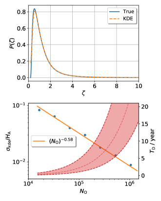
Figure 1: Upper panel:the solid line is the underlying distribution of amplitude $\zeta$ defined following Eq. (9), and the dashed line is the KDE reconstruction from $4.5\times 10^{5}$ merger events detected by the detector network, where $\zeta$ is shown in units of $M_{\odot}^{5/6}{\rm Gpc}^{-1}$. Lower panel:the dots denote the fractional deviation of KDE reconstructed SGWB spectral density and the solid line is a power-law fit $\sigma_{\rm kde}/H_{\rm A}\propto N_{\rm O}^{-0.58}$. The shadowed area denotes the uncertainty in the amount of mergers we expect the ground-based detectors to record in a given running time $T_{\rm D}$, where the thin/dashed line in the center is the fiducial model we use in this work and the two thick/dashed lines correspond to merger rate density $R_{0}=65^{+75}_{-34}\ {\rm Gpc}^{-3}{\rm yr}^{-1}$ [68].

4 Estimating the Extragalactic BWD Foreground

Starting from the mHz range the galactic BWDs will be resolved by LISA, so that the main sources of SGWs are extragalactic BWDs [38] and compact binaries (BBHs, BNSs, and BHNSs) . As the compact binary foreground can be estimated with ground-based GW detections and cleaned accordingly, let us examine the detection of SGWs from extragalactic BWDs in the absence of primordial waves.

For simplicity, let us consider two concentric LISA detectors with output $s_{d}(t)=h_{d}(t)+n_{d}(t)$ ($d=1,2$), with $h_{d}$ and $n_{d}$ denoting the gravitational strain and the intrinsic noise in detector $d$, respectively. The case with a single detector is discussed in the C. The SGWs signal can be measured by cross-correlating outputs from two detector because the detector noises $n_{1}$ and $n_{2}$ are not correlated, while the GW signals $h_{1}$ and $h_{2}$ are correlated. In the Fourier domain, the cross-correlation estimator is written as [65]

$$\hat{X}=\int_{-\infty}^{\infty}df\int_{-\infty}^{\infty}df^{\prime}\delta_{T}(f-f^{\prime})s^{*}_{1}(f)s_{2}(f^{\prime})Q(f)\ ,$$ (13)

where $\delta_{T}(f):=\sin(\pi fT)/(\pi f)$ is a finite-time approximation to the $\delta$-function, $T$ is the running time of the two detectors and $Q(f)$ is a filter function. For later convenience, we define

$$\braket{H_{x}(f)}_{a}^{b} :=\int_{a}^{b}H_{x}(f)\mathcal{R}_{12}(f)Q(f)df\ ,$$ (14)

$$\braket{H_{x}(f)}_{[a,b]}^{[b,c]} :=\braket{H_{x}(f)}_{a}^{b}-\braket{H_{x}(f)}_{b}^{c}\ ,$$

where

$$\mathcal{R}_{12}(f)=\int\frac{d\hat{\Omega}}{4\pi}e^{i2\pi f(\vec{x}_{1}-\vec{x}_{2})\cdot\hat{\Omega}}\sum_{A}F_{1}^{A*}(\hat{\Omega},f)F_{2}^{A}(\hat{\Omega},f)\ ,$$

is the overlap reduction function of the detectors, with $\vec{x}_{1,2}$ being the detector locations. Here we assume two concentric LISA detectors which form a hexagonal pattern [72]. The mean value and variance of estimator $\hat{X}$ turn out to be [65]

$$\braket{\hat{X}} =T\braket{H(f)}_{0}^{\infty}\ ,$$ (15)

$$\sigma_{X}^{2} \approx\frac{T}{2}\int_{0}^{\infty}P_{\rm n}^{2}(f)|Q(f)|^{2}df\ ,$$

where $P_{\rm n}(f)$ is the detector noise spectral density [73]. In the ideal case of zero foreground, we can extract the primordial signal directly using the estimator (15). With the optimal filter $Q(f)=H(f)\mathcal{R}_{12}^{*}(f)/P_{\rm n}^{2}(f)$, we obtain the maximized signal-to-noise ratio (SNR)

$${\rm SNR}_{\rm ideal}=\sqrt{2T\int_{0}^{\infty}\frac{H^{2}(f)}{P_{\rm n}^{2}(f)}|\mathcal{R}_{12}(f)|^{2}df\ .}$$ (16)

The presence of astrophysical foreground of BBHs and galactic BWDs makes the problem more complicated. In the LISA band, the foreground is dominated by the GW emission from galactic BWDs, of which high-frequency binaries can be completely resolved and subtracted in the LISA mission time [59]. And we need to design an estimator with the BBHs foreground subtracted using the KDE reconstruction. The spectral density $H_{\rm A}(f)$ of the BBH foreground is known as a power law, while the spectral density of galactic BWD foreground depends on their orbital distributions. In the following discussion, we will confine our analysis to the frequency range $f\geq f_{\min}=5$ mHz, where galactic BWD foreground can be cleaned up and $H(f)\simeq H_{\rm BWD}^{\rm ext}(f)+H_{\rm A}(f)$ to a good approximation.

The spectral density of the astrophysical foreground from compact binaries $H_{\rm A}(f)$ can be estimated with $H_{\rm kde}(f)$ elaborated in the previous section. From Eq. (15), we define an estimator of the extragalactic BWD foreground as

$$\hat{Y}=\hat{X}-T\braket{H_{\rm kde}(f)}_{f_{\rm min}}^{f_{\rm max}}\ ,$$ (17)

with expectation value and variance

$$\braket{\hat{Y}} =Y_{\rm BWD}^{\rm ext}+T\braket{H_{\rm A}(f)-H_{\rm kde}(f)}_{f_{\rm min}}^{f_{\rm max}}\ ,$$ (18)

$$\sigma_{Y}^{2} =\frac{T}{2}\int_{f_{\rm min}}^{f_{\rm max}}P_{\rm n}^{2}(f)|Q(f)|^{2}df\ ,$$

where $Y_{\rm BWD}^{\rm ext}=T\braket{H_{\rm BWD}^{\rm ext}(f)}_{f_{\rm min}}^{f_{\rm max}}$ and $f_{\rm max}=1$ Hz. Therefore we have $Y_{\rm BWD}^{\rm ext}=\hat{Y}\pm\sigma_{Y}(\rm stat.)\pm\sigma_{\rm A}(\rm syst.)$, where $\sigma_{Y}\propto\sqrt{T}$ is the statistical uncertainty due to detector noise and $\sigma_{\rm A}=T\braket{\sigma_{\rm kde}H_{\rm A}(f)}_{f_{\rm min}}^{f_{\rm max}}$ is the systematic bias due to the limited accuracy of the foreground measurement. Consequently, the SNR of estimator $\hat{Y}$, ${\rm SNR}_{\hat{Y}}=Y_{\rm BWD}^{\rm ext}/\sqrt{\sigma_{Y}^{2}+\sigma_{\rm A}^{2}}$, scales as $\sqrt{T}$ for small $T$, and saturates at $Y_{\rm BWD}^{\rm ext}/\sigma_{\rm A}$ in the large $T$ limit.

Without the multi-band cleaning, the influence of BBH foreground may be removed by using its frequency dependence. For later convenience, we first define a binned estimator

$$\hat{X}_{\mathcal{C}}:=\int_{f\in\mathcal{C}}df\int_{f^{\prime}\in\mathcal{C}}df^{\prime}\delta_{T}(f-f^{\prime})s^{*}_{1}(f)s_{2}(f^{\prime})Q(f)\ ,$$ (19)

and also define an estimator $\hat{Z}$:

$$\hat{Z}=\hat{X}_{\mathcal{C}_{1}}-\hat{X}_{\mathcal{C}_{2}}\ ,$$ (20)

where $\mathcal{C}_{1}=[f_{\rm min},f_{*}],\mathcal{C}_{2}=[f_{*},f_{\rm max}]$, and $f_{*}$ is determined by the constraint that the influence of astrophysical foreground is removed $\braket{H_{\rm A}(f)}_{\mathcal{C}_{1}}^{\mathcal{C}_{2}}=0$. The mean value and the variance of $\hat{Z}$ are

$$\braket{\hat{Z}} =T\braket{H_{\rm BWD}^{\rm ext}(f)}_{\mathcal{C}_{1}}^{\mathcal{C}_{2}}\ ,$$ (21)

$$\sigma_{Z}^{2} =\frac{T}{2}\int_{f_{\rm min}}^{f_{\rm max}}P_{\rm n}^{2}(f)|Q(f)|^{2}df\ .$$

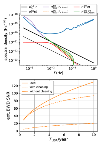
Figure 2: Measuring the SGWs from extragalactic BWDs $H_{\rm BWD}^{\rm ext}(f)$. Upper panel: the spectral densities of effective LISA detector noise $S_{\rm n}(f)$ (blue), BBH foreground $H_{\rm A}(f)$ (thick black) and residual foreground $\sigma_{\rm A}(f)$ after cleaning (thin black), unresolved low-frequency/high-frequency BWD foreground $H_{\rm BWD}(f)$ (purple/orange) [38, 74, 59], and reconstructed high-frequency BWD foreground $H_{\rm BWD}^{\rm ext}(f)$ (green shadow), and a primordial SGWB $H_{\rm P}(f)$ from [75] (red). Lower panel: SNRs of different estimators for the high-frequency extragalactic BWD foreground, where the BBH foreground cleaning increases the detection sensitivity by a factor $4\sim 7$. We also examined less optimistic scenarios of foreground cleaning with $2$ CE-like detectors, and we find the SNR (dashed line) decreases by maximally $\sim 15\%$.

In the upper panel Fig. 2, we present the spectral densities of LISA detector noise, stochastic GW foreground from various sources, and the residual foreground ($\sigma_{\rm kde}/H_{\rm A}=1.3\%$) of compact binaries. In the lower panel, we show the SNRs of extragalactic BWD SGWs with spectral density $H_{\rm BWD}^{\rm ext}(f)$ [38, 59]. Notice that without the compact binary foreground cleaning, the BWD background can still be computed by utilizing the spectral shape of the foreground [Eq. (20)], albeit with much worse sensitivity. Such comparison is shown by the two dashed lines in the figure, where the foreground cleaning [Eq. (17)] increases the detection sensitivity by a factor of $4\sim 7$. In the same figure, the solid line depicts the SNR of an ideal case assuming there was no foreground contamination from compact binaries.

With the presence of primordial SGWB, which is well motivated from various early universe processes, the above analysis can be interpreted as a measurement of a combined signal of the extragalactic BWD foreground and the primordial SGWB.

5 Estimating the Primordial SGWB

The discussion in the previous section provides a way to constrain $H_{\rm P}(f)+H_{\rm BWD}^{\rm ext}(f)$. In order to measure the primordial component $H_{\rm P}(f)$ to probe the early universe, the shape of $H_{\rm BWD}^{\rm ext}(f)$ must be known with certain precision. Unlike BBHs, BWDs of various masses and types may merge in the LISA band so that the mass distribution may have explicit frequency dependence. The resulting stochastic background deviates from simple power laws at high frequencies (see Fig. 2). A detailed theoretical study can be found in Ref. [38], which shows that there is a large uncertainty in the amplitude of the extragalactic BWD foreground, while the shape is insensitive to the astrophysical uncertainties. In this work, we propose to remove the extragalactic BWD foreground via its frequency dependence, i.e., spectral shape,  which can be either modeled as in Ref. [38] or reconstructed from the individually resolved galactic BWDs shown in Fig. 3 and in B. We find the shape uncertainties calculated from the above two methods are comparable and display similar frequency dependence. It is promising to test the (in)consistency of the two in the LISA era.

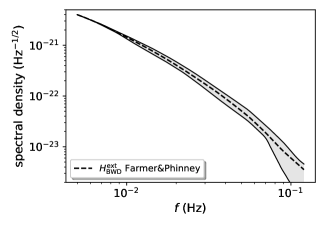
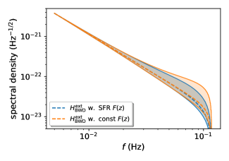
Figure 3: The shape of spectral density $H_{\rm BWD}^{\rm ext}(f)$ can be modeled (left panel) or reconstructed from resolvable galactic BWDs (right panel), where we have normalized the amplitude of $H_{\rm BWD}^{\rm ext}(f)$ at $f=5$ mHz. In the left panel, we have used the variation from the optimistic foreground to the pessimistic foreground calculated in Ref. [38] to quantify the shape uncertainty. As shown in the right panel, the reconstructed $H_{\rm BWD}^{\rm ext}(f)$ is insensitive to the formation rate $\mathcal{F}(z)$ of high-frequency BWDs. The blue line is the result of setting $\mathcal{F}(z)$ equal to the observed star formation rate [76], and the orange line is the result of constant $\mathcal{F}(z)$ (see B for calculation details). The blue and orange shadows are the corresponding statistic uncertainties of reconstruction due to limited number of resolvable galactic BWDs.

With the shape information of $H_{\rm BWD}^{\rm ext}(f)$, we can remove the extragalactic BWD foreground using its frequency dependence. Similar to estimator $\hat{Y}$, we can define estimator

$$\hat{U} =\hat{X}_{\mathcal{C}_{1}}-\hat{X}_{\mathcal{C}_{2}}-T\braket{H_{\rm kde}}_{\mathcal{C}_{1}}^{\mathcal{C}_{2}}\ ,$$ (22)

where $\mathcal{C}_{1}=[f_{\rm min},f_{*}],\mathcal{C}_{2}=[f_{*},f_{\rm max}]$, $f_{*}$ is determined by the constraint that the influence of extragalactic BWD foreground is removed $\braket{H_{\rm BWD,recon.}^{\rm ext}}_{\mathcal{C}_{1}}^{\mathcal{C}_{2}}=0$. The mean value and the variance of $\hat{U}$ are

$$\braket{\hat{U}} =T\braket{H_{\rm P}+H_{\rm BWD}^{\rm ext}+H_{\rm A}-H_{\rm kde}}_{\mathcal{C}_{1}}^{\mathcal{C}_{2}}\ ,$$ (23)

$$\sigma_{U}^{2} =\frac{T}{2}\int_{f_{\rm min}}^{f_{\rm max}}P_{\rm n}^{2}(f)|Q(f)|^{2}df\ ,$$

Similar to estimator $\hat{Y}$, we have $U_{\rm P}:=T\braket{H_{\rm P}}_{\mathcal{C}_{1}}^{\mathcal{C}_{2}}=\hat{U}\pm\sigma_{U}(\rm stat.)\pm\sigma_{\rm BWD}(\rm syst.)\pm\sigma_{\rm A}(\rm syst.)$, where $\sigma_{U}\propto\sqrt{T}$ is the statistical uncertainty due to detector noise, and two systematic terms $\sigma_{\rm BWD}$ and $\sigma_{\rm A}$ are the uncertainty of $T\braket{H_{\rm BWD,recon.}^{\rm ext}}_{\mathcal{C}_{1}}^{\mathcal{C}_{2}}$ (Fig. 3) and $T\braket{\sigma_{\rm kde}H_{\rm A}}_{\mathcal{C}_{1}}^{\mathcal{C}_{2}}$ (Fig. 1), respectively.

Similar to estimator $\hat{Z}$, both the influence of the extragalactic BWD foreground and the BBH foreground can be removed via their frequency dependence without multi-band foreground cleaning. We can define estimator

$$\hat{V}=\left(\hat{X}_{\mathcal{C}_{1}}-\hat{X}_{\mathcal{C}_{2}}\right)-\left(\hat{X}_{\mathcal{C}_{3}}-\hat{X}_{\mathcal{C}_{4}}\right)\ ,$$ (24)

where $\mathcal{C}_{1,..,4}$ are 4 non-overlapped frequency bins and are determined by the constraint that both the extragalactic BWD foreground and the BBH foreground are removed. The mean value and the variance of $\hat{V}$ are

$$\braket{\hat{V}} =T\braket{H_{\rm P}+H_{\rm BWD}^{\rm ext}}_{\mathcal{C}_{1}}^{\mathcal{C}_{2}}-T\braket{H_{\rm P}+H_{\rm BWD}^{\rm ext}}_{\mathcal{C}_{3}}^{\mathcal{C}_{4}}\ ,$$ (25)

$$\sigma_{V}^{2} =\frac{T}{2}\int_{f_{\rm min}}^{f_{\rm max}}P_{\rm n}^{2}(f)|Q(f)|^{2}df\ ,$$

We have $V_{\rm P}:=T\braket{H_{\rm P}}_{\mathcal{C}_{1}}^{\mathcal{C}_{2}}-T\braket{H_{\rm P}}_{\mathcal{C}_{3}}^{\mathcal{C}_{4}}=\hat{V}\pm\sigma_{V}(\rm stat.)\pm\sigma_{\rm BWD}(syst.)$, where $\sigma_{V}$ is the uncertainty due to detector noise and $\sigma_{\rm BWD}$ is the uncertainty of $T\braket{H_{\rm BWD}^{\rm ext}}_{\mathcal{C}_{1}}^{\mathcal{C}_{2}}-T\braket{H_{\rm BWD}^{\rm ext}}_{\mathcal{C}_{3}}^{\mathcal{C}_{4}}$.

For illustration purpose, we consider an example with SGWB generated by bubble collisions during a first order phase transition [75]:

$$H_{\rm P}(f)=\frac{10^{-42}}{1+(f/0.01{\rm Hz})^{4}}\ {\rm Hz}^{-1}\quad{\rm i.e.,}\quad\Omega_{\rm GW}(f)=2.6\times 10^{-12}\frac{(f/0.01{\rm Hz})^{3}}{1+(f/0.01{\rm Hz})^{4}}.$$ (26)

In the left panel of Fig. 4, we show the SNR $U_{\rm P}/\sqrt{\sigma_{U}^{2}+\sigma_{\rm BWD}^{2}+\sigma_{\rm A}^{2}}$ of estimator $\hat{U}$ (solid lines), and the SNR $V_{\rm P}/\sqrt{\sigma_{V}^{2}+\sigma_{\rm BWD}^{2}}$ of estimator $\hat{V}$ (dashed lines), as functions of LISA running time, where $\sigma_{\rm BWD}$ is calculated from the reconstructed shape uncertainty (blue contour in Fig. 3). Without the foreground cleaning (estimator $\hat{V}$), even if we roughly know the spectral shapes of $H_{\rm A}(f)$ and $H_{\rm BWD}^{\rm ext}(f)$, the sensitivity on primordial waves is negligible because of their degeneracy with the SGWB. However, after removing the compact binary foreground (estimator $\hat{U}$), we find that the sensitivity to the primordial waves is greatly enhanced beyond one order of magnitude. The measurement of compact binary foreground and associated multiband cleaning becomes the critical factor that enables the detection of primordial waves. The reconstruction uncertainty of the extragalactic BWD foreground $H_{\rm BWD}^{\rm ext}(f)$ mildly degrades the LISA sensitivity by $5\%\sim 50\%$ depending on the LISA running time. In the right panel, we show the minimum energy $\Omega_{\rm GW}(f)$ of SGWB with the same shape of the example SGWB [Eq. (26)] that can be detected by LISA with $\geq 5\sigma$ confidence level assuming observation time of $5$ years.

The example primordial SGWB above in high-frequency range

$$\Omega_{\rm GW}(f)\simeq 1.0\times 10^{-15}\left(\frac{25\ {\rm Hz}}{f}\right)\ ,$$ (27)

might also be constrained directly by ground based detectors. The current best constraint on SGWB from LIGO is $\Omega_{\rm GW}(f=25\ {\rm Hz})\lesssim 10^{-7}$ (8 orders of magnitude louder than the example signal) at $95\%$ confidence level [77]. Third-generation detectors are expected to be sensitive to primordial SGWB at the level of $\Omega_{\rm GW}(f=25\ {\rm Hz})\simeq 10^{-13}$ (2 orders of magnitude louder) assuming 5 years of observation [57]. As shown in Fig. 4, the example signal is expected to be detected by LISA in combination with the multi-band foreground cleaning with SNR=$4\sim 6$ assuming 5 years of LISA observation, whereas the LISA sensitivity degrades by about two orders of magnitude without the multi-band foreground cleaning and LISA could be sensitive to the example signal if it was $>20$ times louder.

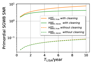
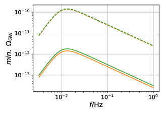
Figure 4: Left panel shows SNRs of different estimators for the fiducial primordial SGWB (Eq.[26]), assuming $H_{\rm BWD}^{\rm ext}(f)$ is either known (orange, $\sigma_{\rm BWD}=0$) or to be reconstructed (green, $\sigma_{\rm BWD}\neq 0$). Right panels shows the minimum energy $\Omega_{\rm GW}(f)$ of SGWB that can be detected by LISA with $\geq 5\sigma$ confidence level assuming observation time of 5 years.

6 Discussion

In the main text, we have assumed that all the galactic BWDs with $f>5$ mHz can be completely substracted from the foreground [60]. In fact, there are more complexities in BWD systems that makes the GW emission hard to be accurately modeled, including accretion when the binary separation is small enough and BWDs in three-body systems. In a BWD system, a WD star is expected to fill the Roche lobe if the binary separation is less than $0.1R_{\odot}$ [38], when the GW frequency $f_{\rm GW}\gtrsim 0.1$ Hz. Therefore accretion between close BWDs might not important considering the small number of BWDs (at most a few [59]) and the large uncertainty of the BWD foreground in this frequency range (Fig. 3). Despite of many N-body simulations of compact objects in dynamical formation channels in the last a couple years, the fraction of BWDs in three-body systems is unknown and there is no accurate model for their GW emission. If a large fraction of BWDs are confirmed in three-body systems by LISA, more accurate models are necessary for the purpose of foreground cleaning.

For all the estimators, we have assumed an BBH foreground with a simple power-law spectral density $H_{\rm A}(f)\propto f^{-7/3}$, which is true only if binaries have zero eccentricity. In the case of mildly eccentric binaries, the spectral density has a more complicated frequency dependence, which deviates from the simple power-law by $\lesssim 50\%$ for BBHs with eccentricity $e\lesssim 0.2$ [78, 79]. In addition, highly eccentric binaries formed through direct captures [80], as sources for ground-based detectors, are born at frequencies higher than those spanned by the LISA band. Therefore it is important to understand the eccentricity distribution of the BBHs for correctly determining the foreground spectral density in the LISA band.

Currently it is believed that there are two main formation channels: field binary evolution and dynamical formation in a dense stellar environment. While BBHs from the former channel are expected to have negligible eccentricities, dynamical formation has the potential to produce BBHs with high eccentricities. As implied by simulations done in Refs. [80, 81], a non-negligible fraction ($\sim 28\%\times 20\%=5.6\%$) of dynamically formed BBHs in dense globular clusters have large eccentricities ($e_{0.01\ {\rm Hz}}\gtrsim 0.1$ or $e_{10\ {\rm Hz}}\gtrsim 10^{-4}$) in the LISA band, and a even larger fraction ($\sim 12\%$) of BBHs are born with larger eccentricities ($e_{10\ {\rm Hz}}\gtrsim 10^{-3}$ ) and never enter the LISA band. The latter ones can be readily measured by CE/ET which can distinguish mergers with eccentricities $e_{10\ {\rm Hz}}\geq 1.7\times 10^{-4}$ [82], so that they will not affect the foreground estimation. As a result, we expect $H_{\rm A}(f)$ to have $\sim 0.5\times 5.6\%\times F_{\rm dy}$ deviation from the circular approximation, where $F_{\rm dy}$ is the fraction of BBHs born in the dynamical channel. If dynamical formation is a sub-dominant channel (say, $F_{\rm dy}<0.4$), the deviation is likely at sub-percent level and can be safely ignored for our purpose. On the other hand, the loud BBH events detected by LISA may also provide us information about eccentricity distribution in the LISA band [83, 84, 85, 79]. Last but not least, another space-borne detector Tianqin is designed to be more sensitive to GWs at higher frequencies (than that of LISA)[86] where the astrophysical foreground is weaker, therefore we expect Tianqin to open another window to probing the primordial SGWB.

In summary, foreground cleaning is a complicated problem and will be a critical factor for detecting the primordial SGWB, one of the most rewarding scientific goals of space missions. A glimpse in this paper does not clean up all the complexities and more effort should be devoted into it. Previous research about detecting various primordial GW signals without considering astrophysical foregrounds or with idealized foreground cleaning should be reexamined.

Appendix A BBH Foreground cleaning by event-based subtraction

In the main text, we reconstructed the underlying distribution of BBH mergers from all the mergers recorded by the CE following the statistical approach. Now we explore the foreground measurement of event-to-event approach . Assume the LISA runs from $-T/2$ to $T/2$, and the CE runs from $-T/2$ to $-T/2+T_{\rm CE}$. For each BBH in the LISA band, we expect to detect its merger after some time $t$ in the CE band, where $t$ is determined by the GW frequency evolution equation [67]

$$\frac{dt}{df}=\frac{5}{96\pi^{8/3}}\frac{f^{-11/3}}{[GM_{c}(1+z)]^{5/3}}\ ,$$ (28)

and we can add up the constribution to the LISA band foreground from BBHs which merger during the CE running phase,

$$\hat{H}_{\rm A}(f)|_{\rm CE}=\frac{1}{T}\sum_{i}\left(|h_{+}(f)|^{2}+|h_{\times}(f)|^{2}\right)_{i}\Theta_{T}^{i}(f)\ ,$$

where $i$ runs over all mergers detected by the CE. If the CE runs for a infinitely long time $T_{\rm CE}\rightarrow\infty$, $\hat{H}_{\rm A}(f)|_{\rm CE}\rightarrow\hat{H}_{\rm A}(f)$. For a finite CE running time, only a fraction of BBHs in the LISA band will evolve into merger phase and the expectation value turns out to be

$$\braket{\hat{H}_{\rm A}(f)}{{}_{\rm CE}} =\int_{z=z_{\rm min}(f,M_{c})}^{z=\infty}\int_{M_{\rm c,min}}^{M_{\rm c,max}}\sum_{A}|h_{A}(f)|^{2}$$ (29)

$$\times\frac{R(z)}{1+z}dV_{c}(z)p(M_{c})dM_{c}\ ,$$

where $z_{\rm min}(f,M_{c})$ is determined by Eq. (28)

$$T_{\rm CE}=\frac{15}{768\pi^{8/3}}\frac{f^{-8/3}}{[GM_{c}(1+z_{\rm min})]^{5/3}}\ ,$$ (30)

where we have used the fact that the BBH merger frequency is well above the LISA band frequency $f$.

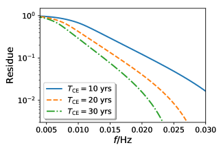
Figure 5: Performance of foreground cleaning with event-based subtraction.

In Fig. 5, we show the residue fraction after the event-to-event cleaning $1-\braket{\hat{H}_{\rm A}(f)}{{}_{\rm CE}}/\braket{\hat{H}_{\rm A}(f)}$ given a finite running CE time ($T_{\rm CE}=10,20,30$ years). It takes longer time for binaries of lower frequency to merge, therefore lower-frequency foreground cleaning is slower. With the CE running for $10$ years, the astrophysical foreground can be cleaned to percent level for $f\gtrsim 0.03$ Hz. Therefore the foreground cleaning of distribution-based approach is more efficient than that of event-based approach.

Appendix B Stochastic GWs from Binary White Dwarfs

Similar to BBHs, the spectral density of the Binary White Dwarf (BWD) foreground averaged over time period $[-T/2,T/2]$ is also

$$\hat{H}_{\rm BWD}(f)=\frac{1}{T}\sum_{i}\left(|h_{+}(f)|^{2}+|h_{\times}(f)|^{2}\right)_{i}\Theta_{T}^{i}(f)\ ,$$ (31)

where $f$ is a frequency in the LISA band. Unlike BBHs, BWDs merge in the LISA band, and this results in some frequency dependence of the expectation value $\braket{\frac{1}{T}\sum_{i}\Theta_{T}^{i}(f)}$. This extra frequency dependence drives $H_{\rm BWD}(f)$ off the power law $f^{-\frac{7}{3}}$ and it is hard to calculate from first principle.

According to simulations performed in Ref. [59], all the high-frequency (say $f>5$ mHz) galactic BWDs are expected to be resolved in the LISA mission time. From these BWDs, we can construct a normalized spectral density,

$$H_{D}(f)\propto\frac{1}{T}\sum_{i}\left(\sum_{A}|h_{A}(f)|^{2}D_{\rm L,eff}^{2}\right)_{i}\Theta_{T}^{i}(f)\ ,$$ (32)

where all the effective distance information has been removed, $D_{\rm L,eff}=D_{\rm L}/\sqrt{\cos^{2}\imath+(\frac{1+\cos^{2}\imath}{2})^{2}}$. The normalized spectral density $H_{D}(f)$ is actually a statistical property of the galactic BWDs and can be used to reconstruct the extragalactic BWD foreground if the population of galactic BWDs does not deviate significantly from average extraglatic BWDs. The spectral density of extragalactic BWD foreground is then calculated as

$$H_{\rm BWD}^{\rm ext}(f)\propto\int_{0}^{V_{c}(z_{*})}\frac{H_{D}(f(1+z))}{D_{\rm L}^{2}(z)}\frac{\mathcal{F}(z)}{1+z}dV_{c}(z)\ ,$$ (33)

where $\mathcal{F}(z)$ is the formation rate of high-frequency BWDs. Though the accurate form of $\mathcal{F}(z)$ is unknown, as shown in Fig. 3, it has little influence on the shape of $H_{\rm BWD}^{\rm ext}(f)$.

There are two major sources of the uncertainty of $H_{\rm BWD}^{\rm ext}(f)$ reconstruction from resolvable galactic BWDs, one is statistic uncertainty due to limited number of galactic BWDs and the other is the uncertainty in the formation rate $\mathcal{F}(z)$. Following [59], we assume the total number of resolvable high-frequency galactic BWDs is $10^{4}$, and these BWDs roughly satisfy a power-law distribution $dN/df\propto f^{-4.8}$ in the frequency range $[5,120]$ mHz. For the chirp mass, we assume a Gaussian distribution with mean value $0.4M_{\odot}$ and standard deviation $0.1M_{\odot}$. To examine how much uncertainty in $H_{\rm BWD}^{\rm ext}(f)$ is introduced by the uncertainty of $\mathcal{F}(z)$, we consider two $\mathcal{F}(z)$ functions: one is the star formation rate [76], and the other is a constant. For each $F(z)$, we simulate 100 realizations of resolved galactic BWDs, for each of which we fit $\log H_{D}-\log f$ with a 2nd-degree polynomial and calculate $H_{\rm BWD}^{\rm ext}(f)$ from Eq. (33). The true spectral density $H_{\rm BWD}^{\rm ext}(f)$ along with the reconstruction uncertainties are shown in Fig. 3, which clearly shows the shape of $H_{\rm BWD}^{\rm ext}(f)$ is insensitive to $\mathcal{F}(z)$ and the reconstruction uncertainty is dominated by the statistic uncertainty.

The reconstruction uncertainty is small ($\sim 1\%$) at low frequencies where a large number of BWDs reside, and is much larger ($\sim 200\%$) at high frequencies. However, this method relies on the assumption that the population of galactic BWDs does not deviate significantly from average extragalactic BWDs. This assumption may be tested with population synthesis studies and further examined by comparing the observationally reconstructed background with the prediction in Ref. [38].

Appendix C One detector, two channels

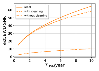
Figure 6: Measuring the extragalactic BWD foreground using two channels of a single LISA detector.

In the main text, we have outlined the foreground cleaning with KDE reconstruction assuming two LISA detectors for convenience, where the stochastic GWs can be separated from detector noise by cross-correlating the two detector outputs. For the proposed LISA mission, there will be a single detector and we may detect the SGWB by utilizing the “null” channel which is blind to GW signals for detector noise calibration, in combination with the normal Michelson (m) channel [87]. In reality, a good approximation to the ideal null channel is the symmetrized Sagnac (ss) channel whose response function $\mathcal{R}_{\rm ss}(f)$ is much smaller than that of the Michelson channel $\mathcal{R}_{\rm m}(f)$ especially in the lower frequency range [88, 89, 90, 91]. In combination with the outputs of the two channels, it is natural to write the SGWB estimator as

$$\hat{X} =\int_{-\infty}^{\infty}df\int_{-\infty}^{\infty}df^{\prime}\delta_{T}(f-f^{\prime})$$ (34)

$$\times\left[s^{*}_{\rm m}(f)s_{\rm m}(f^{\prime})-W(f)s^{*}_{\rm ss}(f)s_{\rm ss}(f^{\prime})\right]Q(f)\ ,$$

where $W(f)=P_{{\rm m}}(f)/P_{{\rm ss}}(f)$, with $P_{{\rm ss}}(f)$ and $P_{{\rm m}}(f)$ being the detector noise spectral density of two channels [73]. The mean value and variance are

$$\braket{\hat{X}} =T\int_{0}^{\infty}H(f)\left[\mathcal{R}_{\rm m}(f)-W(f)\mathcal{R}_{\rm ss}(f)\right]Q(f)df,$$

$$\sigma_{X}^{2} \approx 2T\int_{0}^{\infty}\left[P^{2}_{{\rm m}}(f)-W(f)|P_{{\rm m},{\rm ss}}(f)|^{2}\right]|Q(f)|^{2}df\ .$$

where $P_{{\rm m},{\rm ss}}(f)$ is cross power of noises in the two channels. In the similar way, we can write the estimators $\hat{Y}$ and $\hat{Z}$ as in the case of two LISA detectors. We show the SNRs of different estimators for the extragalactic BWD foreground in Fig. 6. As in the two-detectors case, the BBH foreground cleaning increases the LISA sensitivity by a factor $4\sim 7$. Compared with the case of two detectors, the SNRs of different estimators here turn out to be smaller by a factor $\sim 2$.

References

References

- [1] Caprini C and Figueroa D G 2018 Classical and Quantum Gravity 35 163001 (Preprint 1801.04268)
- [2] Christensen N 2019 Reports on Progress in Physics 82 016903 (Preprint 1811.08797)
- [3] Guth A H 1981 Phys. Rev. D 23(2) 347–356 URL https://link.aps.org/doi/10.1103/PhysRevD.23.347
- [4] Linde A D 1982 Physics Letters B 108 389–393
- [5] Starobinskiǐ A A 1979 Soviet Journal of Experimental and Theoretical Physics Letters 30 682
- [6] Turner M S 1997 Phys. Rev. D 55(2) R435–R439 URL https://link.aps.org/doi/10.1103/PhysRevD.55.R435
- [7] Easther R and Lim E A 2006 JCAP 4 010 (Preprint astro-ph/0601617)
- [8] Easther R, Giblin J T and Lim E A 2007 Phys. Rev. Lett. 99(22) 221301 URL https://link.aps.org/doi/10.1103/PhysRevLett.99.221301
- [9] Barnaby N, Pajer E and Peloso M 2012 Phys. Rev. D 85(2) 023525 URL https://link.aps.org/doi/10.1103/PhysRevD.85.023525
- [10] Cook J L and Sorbo L 2012 Phys. Rev. D 85(2) 023534 URL https://link.aps.org/doi/10.1103/PhysRevD.85.023534
- [11] Kibble T W B 1976 Journal of Physics A Mathematical General 9 1387–1398
- [12] Vilenkin A 1981 Physics Letters B 107 47–50
- [13] Hogan C J and Rees M J 1984 Nature 311 109–114
- [14] Caldwell R R and Allen B 1992 Phys. Rev. D 45 3447–3468
- [15] Vilenkin A and Shellard E P S 1994 Cosmic strings and other topological defects
- [16] Damour T and Vilenkin A 2000 Phys. Rev. Lett 85 3761–3764 (Preprint gr-qc/0004075)
- [17] Damour T and Vilenkin A 2001 Phys. Rev. D 64 064008 (Preprint gr-qc/0104026)
- [18] Jeannerot R, Rocher J and Sakellariadou M 2003 Phys. Rev. D 68(10) 103514 URL https://link.aps.org/doi/10.1103/PhysRevD.68.103514
- [19] Damour T and Vilenkin A 2005 Phys. Rev. D 71(6) 063510 URL https://link.aps.org/doi/10.1103/PhysRevD.71.063510
- [20] Sakellariadou M 2006 Annalen der Physik 15 264–276 ISSN 1521-3889 URL http://dx.doi.org/10.1002/andp.200510186
- [21] Sakellariadou M 2007 Cosmic Strings Lecture Notes in Physics, Berlin Springer Verlag vol 718 ed Unruh W G and Schützhold R p 247 (Preprint hep-th/0602276)
- [22] Siemens X, Mandic V and Creighton J 2007 Phys. Rev. Lett. 98(11) 111101 URL https://link.aps.org/doi/10.1103/PhysRevLett.98.111101
- [23] Turner M S and Wilczek F 1990 Phys. Rev. Lett 65 3080–3083
- [24] Turner M S, Weinberg E J and Widrow L M 1992 Phys. Rev. D 46 2384–2403
- [25] Kosowsky A, Turner M S and Watkins R 1992 Phys. Rev. D 45(12) 4514–4535 URL https://link.aps.org/doi/10.1103/PhysRevD.45.4514
- [26] Kosowsky A, Turner M S and Watkins R 1992 Phys. Rev. Lett. 69(14) 2026–2029 URL https://link.aps.org/doi/10.1103/PhysRevLett.69.2026
- [27] Kamionkowski M, Kosowsky A and Turner M S 1994 Phys. Rev. D 49(6) 2837–2851 URL https://link.aps.org/doi/10.1103/PhysRevD.49.2837
- [28] Caprini C, Durrer R and Servant G 2008 Phys. Rev. D 77(12) 124015 URL https://link.aps.org/doi/10.1103/PhysRevD.77.124015
- [29] Iso S, Serpico P D and Shimada K 2017 Phys. Rev. Lett. 119(14) 141301 URL https://link.aps.org/doi/10.1103/PhysRevLett.119.141301
- [30] Cutting D, Hindmarsh M and Weir D J 2018 Phys. Rev. D 97 123513 (Preprint 1802.05712)
- [31] Kamionkowski M, Kosowsky A and Stebbins A 1997 Phys. Rev. Lett. 78(11) 2058–2061 URL https://link.aps.org/doi/10.1103/PhysRevLett.78.2058
- [32] Seljak U and Zaldarriaga M 1997 Phys. Rev. Lett. 78(11) 2054–2057 URL https://link.aps.org/doi/10.1103/PhysRevLett.78.2054
- [33] Hobbs G, Archibald A, Arzoumanian Z, Backer D, Bailes M, Bhat N D R, Burgay M, Burke-Spolaor S, Champion D, Cognard I, Coles W, Cordes J, Demorest P, Desvignes G, Ferdman R D, Finn L, Freire P, Gonzalez M, Hessels J, Hotan A, Janssen G, Jenet F, Jessner A, Jordan C, Kaspi V, Kramer M, Kondratiev V, Lazio J, Lazaridis K, Lee K J, Levin Y, Lommen A, Lorimer D, Lynch R, Lyne A, Manchester R, McLaughlin M, Nice D, Oslowski S, Pilia M, Possenti A, Purver M, Ransom S, Reynolds J, Sanidas S, Sarkissian J, Sesana A, Shannon R, Siemens X, Stairs I, Stappers B, Stinebring D, Theureau G, van Haasteren R, van Straten W, Verbiest J P W, Yardley D R B and You X P 2010 Classical and Quantum Gravity 27 084013 (Preprint 0911.5206)
- [34] Bender P L, Brillet A, Ciufolini I, Cruise A M, Cutler C J, Danzmann K, Fidecaro F, Folkner W M, Hough J H, Mcnamara P A, Peterseim M, Robertson D I, e Rodrigues M R, Ruediger A, Sandford M, Schilling R, Schutz B, Speake C C, Stebbins R T, Sumner T J, Touboul P, Vinet J Y, Vitale S, Ward H and Winkler W 1998 LISA Pre-Phase A Report
- [35] Sato S, Kawamura S, Ando M, Nakamura T, Tsubono K, Araya A, Funaki I, Ioka K, Kanda N, Moriwaki S, Musha M, Nakazawa K, Numata K, Sakai S i, Seto N, Takashima T, Tanaka T, Agatsuma K, Aoyanagi K s, Arai K, Asada H, Aso Y, Chiba T, Ebisuzaki T, Ejiri Y, Enoki M, Eriguchi Y, Fujimoto M K, Fujita R, Fukushima M, Futamase T, Ganzu K, Harada T, Hashimoto T, Hayama K, Hikida W, Himemoto Y, Hirabayashi H, Hiramatsu T, Hong F L, Horisawa H, Hosokawa M, Ichiki K, Ikegami T, Inoue K T, Ishidoshiro K, Ishihara H, Ishikawa T, Ishizaki H, Ito H, Itoh Y, Kawashima N, Kawazoe F, Kishimoto N, Kiuchi K, Kobayashi S, Kohri K, Koizumi H, Kojima Y, Kokeyama K, Kokuyama W, Kotake K, Kozai Y, Kudoh H, Kunimori H, Kuninaka H, Kuroda K, Maeda K i, Matsuhara H, Mino Y, Miyakawa O, Miyoki S, Morimoto M Y, Morioka T, Morisawa T, Mukohyama S, Nagano S, Naito I, Nakamura K, Nakano H, Nakao K, Nakasuka S, Nakayama Y, Nishida E, Nishiyama K, Nishizawa A, Niwa Y, Noumi T, Obuchi Y, Ohashi M, Ohishi N, Ohkawa M, Okada N, Onozato K, Oohara K, Sago N, Saijo M, Sakagami M, Sakata S, Sasaki M, Sato T, Shibata M, Shinkai H, Somiya K, Sotani H, Sugiyama N, Suwa Y, Suzuki R, Tagoshi H, Takahashi F, Takahashi K, Takahashi K, Takahashi R, Takahashi R, Takahashi T, Takahashi H, Akiteru T, Takano T, Taniguchi K, Taruya A, Tashiro H, Torii Y, Toyoshima M, Tsujikawa S, Tsunesada Y, Ueda A, Ueda K i, Utashima M, Wakabayashi Y, Yamakawa H, Yamamoto K, Yamazaki T, Yokoyama J, Yoo C M, Yoshida S and Yoshino T 2017 The status of DECIGO Journal of Physics Conference Series (Journal of Physics Conference Series vol 840) p 012010
- [36] The LIGO/Virgo Scientific Collaboration 2017 Phys. Rev. Lett. 118 121101 ISSN 10797114
- [37] Lasky P D, Mingarelli C M F, Smith T L, Giblin J T, Thrane E, Reardon D J, Caldwell R, Bailes M, Bhat N D R, Burke-Spolaor S, Dai S, Dempsey J, Hobbs G, Kerr M, Levin Y, Manchester R N, Osłowski S, Ravi V, Rosado P A, Shannon R M, Spiewak R, van Straten W, Toomey L, Wang J, Wen L, You X and Zhu X 2016 Phys. Rev. X 6(1) 011035 URL https://link.aps.org/doi/10.1103/PhysRevX.6.011035
- [38] Farmer A J and Phinney E S 2003 MNRAS 346 1197–1214 (Preprint astro-ph/0304393)
- [39] Marassi S, Schneider R, Corvino G, Ferrari V and Zwart S P 2011 Phys. Rev. D 84(12) 124037 URL https://link.aps.org/doi/10.1103/PhysRevD.84.124037
- [40] Rosado P A 2011 Phys. Rev. D 84(8) 084004 URL https://link.aps.org/doi/10.1103/PhysRevD.84.084004
- [41] Zhu X J, Howell E, Regimbau T, Blair D and Zhu Z H 2011 Astro. Phys. J 739 86 (Preprint 1104.3565)
- [42] Wu C, Mandic V and Regimbau T 2012 Phys. Rev. D 85(10) 104024 URL https://link.aps.org/doi/10.1103/PhysRevD.85.104024
- [43] Zhu X J, Howell E J, Blair D G and Zhu Z H 2013 MNRAS 431 882–899 (Preprint 1209.0595)
- [44] The LIGO/Virgo Scientific Collaboration (LIGO Scientific Collaboration and Virgo Collaboration) 2018 Phys. Rev. Lett. 120(9) 091101 URL https://link.aps.org/doi/10.1103/PhysRevLett.120.091101
- [45] Pieroni M and Barausse E 2020 arXiv e-prints arXiv:2004.01135 (Preprint 2004.01135)
- [46] Sesana A 2016 Phys. Rev. Lett. 116 231102 ISSN 10797114
- [47] Barausse E, Yunes N and Chamberlain K 2016 Physical Review Letters 116 241104 (Preprint 1603.04075)
- [48] Vitale S 2016 Physical Review Letters 117 051102 (Preprint 1605.01037)
- [49] Tinto M and de Araujo J C N 2016 Phys. Rev. D 94 081101 (Preprint 1608.04790)
- [50] Sesana A 2017 Multi-band gravitational wave astronomy: science with joint space- and ground-based observations of black hole binaries Journal of Physics Conference Series (Journal of Physics Conference Series vol 840) p 012018 (Preprint 1702.04356)
- [51] Wong K W, Kovetz E D, Cutler C and Berti E 2018 Phys. Rev. Lett. 121 251102 ISSN 10797114 URL https://doi.org/10.1103/PhysRevLett.121.251102
- [52] Isoyama S, Nakano H and Nakamura T 2018 Progress of Theoretical and Experimental Physics 2018 073E01 (Preprint 1802.06977)
- [53] Carson Z and Yagi K 2019 arXiv e-prints (Preprint 1905.13155)
- [54] Bartolo N, Caprini C, Domcke V, Figueroa D G, Garcia-Bellido J, Chiara Guzzetti M, Liguori M, Matarrese S, Peloso M, Petiteau A, Ricciardone A, Sakellariadou M, Sorbo L and Tasinato G 2016 JCAP 2016 026 (Preprint 1610.06481)
- [55] Abbott B P, Abbott R, Abbott T D, Abernathy M R, Ackley K, Adams C, Addesso P, Adhikari R X, Adya V B, Affeldt C and et al 2017 Classical and Quantum Gravity 34 044001 (Preprint 1607.08697)
- [56] Punturo M et al. 2010 Class. Quant. Grav. 27 194002
- [57] Regimbau T, Evans M, Christensen N, Katsavounidis E, Sathyaprakash B and Vitale S 2017 Phys. Rev. Lett. 118 151105 ISSN 10797114
- [58] Reitze D, LIGO Laboratory: California Institute of Technology, LIGO Laboratory: Massachusetts Institute of Technology, LIGO Hanford Observatory and LIGO Livingston Observatory 2019 BAAS 51 141 (Preprint 1903.04615)
- [59] Lamberts A, Blunt S, Littenberg T B, Garrison-Kimmel S, Kupfer T and Sanderson R E 2019 MNRAS 490 5888–5903 (Preprint 1907.00014)
- [60] Cutler C and Harms J 2006 Phys. Rev. D 73(4) 042001 URL https://link.aps.org/doi/10.1103/PhysRevD.73.042001
- [61] Adams M R and Cornish N J 2014 Phys. Rev. D 89 1–10 ISSN 15507998
- [62] Buonanno A, Sigl G, Raffelt G G, Janka H T and Müller E 2005 Phys. Rev. D 72(8) 084001 URL https://link.aps.org/doi/10.1103/PhysRevD.72.084001
- [63] Lorén-Aguilar P, Isern J and García-Berro E 2009 Astronomy and Astrophysics 500 1193–1205
- [64] Dan M, Rosswog S, Guillochon J and Ramirez-Ruiz E 2011 Astro. Phys. J 737 89 (Preprint 1101.5132)
- [65] Allen B and Romano J D 1999 Phys. Rev. D 59 102001 ISSN 15502368 (Preprint 9710117) URL http://arxiv.org/abs/gr-qc/9710117%0Ahttp://dx.doi.org/10.1103/PhysRevD.59.102001
- [66] Phinney E S 2001 A practical theorem on gravitational wave backgrounds (Preprint astro-ph/0108028)
- [67] Cutler C and Flanagan É E 1994 Phys. Rev. D 49 2658–2697 ISSN 0556-2821 URL https://link.aps.org/doi/10.1103/PhysRevD.49.2658
- [68] The LIGO/Virgo Scientific Collaboration 2018 (Preprint 1811.12940) URL http://arxiv.org/abs/1811.12940
- [69] Ajith P, Hannam M, Husa S, Chen Y, Brügmann B, Dorband N, Müller D, Ohme F, Pollney D, Reisswig C, Santamaría L and Seiler J 2011 Phys. Rev. Lett. 106 241101 ISSN 00319007
- [70] Zhao W and Wen L 2018 Phys. Rev. D 97 64031 ISSN 24700029 URL https://doi.org/10.1103/PhysRevD.97.064031
- [71] Yang H and Martynov D 2018 Phys. Rev. Lett. 121 071102 (Preprint 1803.02429)
- [72] Cornish N J and Larson S L 2001 Class. Quantum Gravity 18 3473–3495 ISSN 02649381 URL http://stacks.iop.org/0264-9381/18/i=17/a=308?key=crossref.8ecd4223d4356daa7a7ff7cf0d3b8aa0
- [73] Robson T, Cornish N and Liug C 2018 Class. Quantum Gravity 36 105011 ISSN 0264-9381 (Preprint 1803.01944) URL https://iopscience.iop.org/article/10.1088/1361-6382/ab1101http://arxiv.org/abs/1803.01944
- [74] Cornish N and Robson T 2017 Galactic binary science with the new LISA design Journal of Physics Conference Series (Journal of Physics Conference Series vol 840) p 012024 (Preprint 1703.09858)
- [75] Caprini C, Durrer R, Konstandin T and Servant G 2009 Phys. Rev. D 79(8) 083519 URL https://link.aps.org/doi/10.1103/PhysRevD.79.083519
- [76] Cole S, Norberg P, Baugh C M, Frenk C S, Bland-Hawthorn J, Bridges T, Cannon R, Colless M, Collins C, Couch W, Cross N, Dalton G, De Propris R, Driver S P, Efstathiou G, Ellis R S, Glazebrook K, Jackson C, Lahav O, Lewis I, Lumsden S, Maddox S, Madgwick D, Peacock J A, Peterson B A, Sutherland W and Taylor K 2001 MNRAS 326 255–273 (Preprint astro-ph/0012429)
- [77] LIGO Scientific and Virgo Collaboration 2019 Phys. Rev. D 100 061101 (Preprint 1903.02886)
- [78] Huerta E A, McWilliams S T, Gair J R and Taylor S R 2015 Phys. Rev. D 92 063010 ISSN 15502368 (Preprint 0108028)
- [79] Randall L and Xianyu Z Z 2019 (Preprint 1907.02283) URL http://arxiv.org/abs/1907.02283
- [80] Rodriguez C L, Amaro-Seoane P, Chatterjee S, Kremer K, Rasio F A, Samsing J, Ye C S and Zevin M 2018 Phys. Rev. D 98 123005 ISSN 24700029 URL https://doi.org/10.1103/PhysRevD.98.123005
- [81] Kremer K, Rodriguez C L, Amaro-Seoane P, Breivik K, Chatterjee S, Katz M L, Larson S L, Rasio F A, Samsing J, Ye C S and Zevin M 2019 Phys. Rev. D 99 63003 ISSN 24700029 URL https://doi.org/10.1103/PhysRevD.99.063003
- [82] Lower M E, Thrane E, Lasky P D and Smith R 2018 Phys. Rev. D 98 083028 ISSN 24700029 URL https://doi.org/10.1103/PhysRevD.98.083028
- [83] Breivik K, Rodriguez C L, Larson S L, Kalogera V and Rasio F A 2016 Astrophys. J. 830 L18 ISSN 2041-8213 URL http://stacks.iop.org/2041-8205/830/i=1/a=L18?key=crossref.eb509bf6b49f24c2aa632eaddbbb9086
- [84] Nishizawa A, Berti E, Klein A and Sesana A 2016 Phys. Rev. D 94(6) 064020 URL https://link.aps.org/doi/10.1103/PhysRevD.94.064020
- [85] Nishizawa A, Sesana A, Berti E and Klein A 2017 Mon. Not. R. Astron. Soc. 465 4375–4380 ISSN 13652966 (Preprint 1606.09295) URL http://arxiv.org/abs/1606.09295http://dx.doi.org/10.1093/mnras/stw2993
- [86] Lu X Y, Tan Y J and Shao C G 2019 Phys. Rev. D 100(4) 044042 URL https://link.aps.org/doi/10.1103/PhysRevD.100.044042
- [87] Romano J D and Cornish N J 2017 Living Reviews in Relativity 20 ISSN 1433-8351 URL http://dx.doi.org/10.1007/s41114-017-0004-1
- [88] Armstrong J W, Estabrook F B and Tinto M 1999 Astro. Phys. J 527 814–826
- [89] Tinto M, Armstrong J W and Estabrook F B 2000 Phys. Rev. D 63 021101 ISSN 15502368
- [90] Cornish N J 2001 Phys. Rev. D 65 022004 ISSN 15502368
- [91] Hogan C J and Bender P L 2001 Phys. Rev. D 64 062002 (Preprint astro-ph/0104266)