Foreground cleaning and template-free stochastic background extraction for LISA

Abstract

Based on the rate of resolved stellar origin black hole and neutron star mergers measured by LIGO and Virgo, it is expected that these detectors will also observe an unresolved Stochastic Gravitational Wave Background (SGWB) by the time they reach design sensitivity. A background from the same class of sources also exists in the LISA band, which will be observable by LISA with signal-to-noise ratio (SNR) $\sim 53$. Unlike the stochastic signal from Galactic white dwarf binaries, for which a partial subtraction is expected to be possible by exploiting its yearly modulation (induced by the motion of the LISA constellation), the background from unresolved stellar origin black hole and neutron star binaries acts as a foreground for other stochastic signals of cosmological or astrophysical origin, which may also be present in the LISA band. Here, we employ a principal component analysis to model and extract an additional hypothetical SGWB in the LISA band, without making any a priori assumptions on its spectral shape. At the same time, we account for the presence of the foreground from stellar origin black holes and neutron stars, as well as for possible uncertainties in the LISA noise calibration. We find that our technique leads to a linear problem and is therefore suitable for fast and reliable extraction of SGWBs with SNR up to ten times weaker than the foreground from black holes and neutron stars, quite independently of the SGWB spectral shape.

1 Introduction

The Laser Interferometer Space Antenna (LISA) Audley:2017drz is a space-based Gravitational Wave (GW) detector scheduled to be launched by ESA, with junior partnership from NASA, around 2034. LISA is currently in Phase A (assessment of feasibility), and among the items that are being investigated is the scientific return as function of the mission design. The LISA observatory will be comprised by three spacecraft trailing the Earth around the Sun (by 10–15 degrees), on an equilateral configuration with arms of about 2.5 million km. Along these arms, laser beams will be exchanged to monitor changes in the proper distance between the free-falling test masses carried by the spacecraft, in order to detect GW signals with frequencies in the mHz band.

The GW sky at such low frequencies is expected to be much more crowded than in the band $\gtrsim 10$–$100$ Hz accessible from the ground TheLIGOScientific:2014jea ; Advanced-Virgo ; Hild:2010id . Indeed, LISA sources are intrinsically long-lived, i.e. they are expected to be active for the whole duration of the mission (which is nominally of 4 yr), and they are foreseen to number in the tens of thousands Audley:2017drz (including resolved sources alone). In more detail, the strongest sources, with Signal to Noise Ratios (SNRs) up to thousands, are expected to be the mergers of massive black hole binaries (with masses $\sim 10^{4}$–$10^{7}M_{\odot}$), which could be between a few and hundreds depending on the (currently unknown) astrophysical formation scenario Sesana2004 ; Sesana2005 ; Barausse2012 ; Klein2016 ; 2019MNRAS.486.4044B . Extreme mass ratio inspirals comprised of a massive black hole (with mass again $\sim 10^{4}$–$10^{7}M_{\odot}$) and a smaller satellite stellar-origin black hole (with mass $\sim 10$–$50M_{\odot}$) or neutron star may also be present, with very uncertain rates ranging from a few up to hundreds per year Babak2017 .

LISA is also guaranteed to be able to observe a handful of white dwarf binaries that have already been observed in the electromagnetic band. These are referred to as “verification binaries” verification , and are just the tip of the iceberg of a much broader population of Galactic and extragalactic white dwarf binaries that are potentially observable with LISA. Indeed, models of this population in the Milky Way predict that LISA should detect the signal of tens of thousands of resolved Galactic white dwarf binaries at low frequencies WD1 ; WD2 ; WD3 ; WD4 ; WD5 . Moreover, even more such sources will not have sufficient SNR to be detectable individually, but will nevertheless constitute a formidable stochastic background signal, which will be potentially strong enough to degrade the mission’s sensitivity at low frequencies, i.e. to act as a foreground for other sources cornish1 ; Adams:2013qma .

After the first LIGO detection of GW150914 Abbott:2016blz , it was realized that binaries of stellar-origin black holes, which merge in the band of existing or future ground based interferometers, will also be detectable in LISA much earlier (by a time ranging from weeks to years) than their merger Sesana:2017vsj (see also Wong:2018uwb ; Gerosa:2019dbe ). While the presence of these sources is a blessing, since their long low frequency inspiral allows for measuring their parameters to high accuracy, thus permitting precise tests of their formation scenario Nishizawa1 ; Nishizawa2 ; Tamanini:2019usx , of General Relativity dipole ; Carson:2019rda ; Gnocchi:2019jzp , and possibly identify their electromagnetic counterparts (if any) caputo_sberna , many of them may not be detectable individually. The unresolved signal from stellar-origin black hole binaries is indeed foreseen to be present in the LIGO/Virgo band too, and should be detected when those detectors reach design sensitivity. Based on the current estimates of this background LIGOScientific:2019vic , its SNR in the LISA band is expected to be around 53 While this is not enough to degrade the detector’s sensitivity to resolved sources (unlike the case of Galactic white dwarf binaries), this unresolved signal is expected to be certainly detectable once all resolved sources have been subtracted, by looking at the auto-correlation of the data residuals.

Unlike the stochastic background from Galactic binaries, however, the background from stellar-origin black holes is expected to be overwhelmingly extra-galactic in origin. As a result, while the unresolved signal from Galactic binaries can for the most part be subtracted by exploiting its yearly modulation (induced by the constellation’s motion around the Sun) and its anisotropy Adams:2013qma , the background from stellar-origin black holes will be (to a very good approximation) isotropic and stationary. This makes its subtraction difficult, and may hamper the detection of other, weaker SGWBs that may be present in the data.

Indeed, one of the most important goals of the LISA mission is the possible detection of SGWBs of exotic origin. While some of these, if present, may be very strong (e.g. stochastic signals from the superradiance driven spin down of the astrophysical black hole population, which may occur in models of fuzzy dark matter Brito1 ; Brito2 or in the presence of exotic physics near the event horizon Barausse:2018vdb ), most signals of cosmological origin are expected to be rather weak. Indeed, it is possible to construct scenarios in which phase transitions in the early Universe Caprini:2019egz , networks of topological defects (e.g. cosmic strings) Auclair:2019wcv and even inflationary constructions Bartolo:2016ami may induce a sufficiently large SGWB to reach the sensitivity of LISA (for a review of these models see for example Caprini:2018mtu and reference therein). However, for these relatively weak signals, the background from stellar-origin black holes will act as a foreground and may jeopardize their detection, unless it is successfully subtracted.

Here, we introduce a template free approach for the detection and reconstruction of the LISA SGWB. Our method is based on a Principal Component Analysis (PCA; or singular value decomposition), and we show that it allows for the simultaneous detection and characterization of the foreground from stellar-origin black holes and a signal of unknown origin and spectral shape. While similar in spirit to Karnesis:2019mph ; Caprini:2019pxz , where template free approaches were also put forward, our technique has the advantage of being very fast, because the determination of the posteriors becomes equivalent to solving a linear problem, and allows for detecting signals up to ten times weaker than the one from stellar-origin black holes.

This paper is organized as follows: in section 2 we describe the procedure to generate our data and the technique on which our analysis hinges. In section 3 we show the results obtained by applying these techniques to a set of mock signals. Finally, in section 4 we draw our conclusions. This work contains two appendices: in appendix A we describe the noise model used in our analyses and in appendix B we discuss the procedure to downsample our data.

2 A principal component analysis for the stochastic background

We start by making the standard simplifying assumption that once all resolved sources have been subtracted, the LISA data (i.e. the residuals) in a given channel are described by a stationary Gaussian process . If we deconvolve the LISA data with the response function of the detector, as described in appendix A, the resulting data $d(t)$ will satisfy

$$\langle d(f)d^{*}(f^{\prime})\rangle=S(f)\delta(f-f^{\prime})\,,$$ (1)

where

$$d(f)=\int_{-\infty}^{\infty}d(t)\exp(-2\pi ift)dt$$ (2)

is the (complex) Fourier transform of the time domain data $d(t)$, $\langle\ldots\rangle$ denotes an ensemble average (i.e. an average over many data realizations), and $S(f)$ is referred to as the (double sided) spectral density of the data $d$ Maggiore:1900zz .

Since LISA samples the data for a finite observation time $T$, the Fourier transform is defined only at discrete frequencies $f_{i}$ (with $i$ the frequency index ranging e.g. from $1$ to $n$) spaced by $\Delta f=1/T$, and eq. 1 becomes

$$\langle d_{i}d^{*}_{j}\rangle=\frac{1}{\Delta f}S(f_{i})\delta_{ij}\,,$$ (3)

where $d_{i}\equiv d(f_{i})$. Since the residuals are Gaussian, the real and imaginary parts of the $d_{i}$ obey a Gaussian distribution with variance set by eq. 3, i.e.

$$p({\rm Re}\,d_{i},{\rm Im}\,d_{i})=\frac{1}{\pi S_{i}}e^{-[({\rm Re}\,d_{i})^{2}+({\rm Im}\,d_{i})^{2}]/S_{i}}\,.$$ (4)

By changing variables to the absolute value ($|d_{i}|$) and phase of the data, one obtains that the phase is uniformly distributed, while $|d_{i}|$ is described by $p(|d_{i}|)=2|d_{i}|e^{-|d_{i}|^{2}/S_{i}}/S_{i}$.

Since different frequencies are uncorrelated, as per eq. 1, the likelihood can be obtained by multiplying the probability distributions of the various sampled frequencies $f_{i}$. In particular, by working not with $|d_{i}|$ but with $D_{i}\equiv|d_{i}|^{2}$, one obtains

$$p(D_{i=1,...,n}|S)=\prod_{i}^{n}\frac{1}{S_{i}}e^{-D_{i}/S_{i}}\,,$$ (5)

for the data in each channel. At a fixed frequency $f_{i}$, the mean value of $D_{i}$ is $\mu_{i}=S_{i}$ and its variance $\sigma^{2}_{i}=\mu_{i}^{2}=S_{i}^{2}$.

We now consider $\bar{D}_{i}$, which we define as the average of $D_{i}$ (with $i$ fixed) over $N\gg 1$ chunks in which we divide the time series. By the central limit theorem, we can approximate the probability distribution function for $\bar{D}_{i}$ with a Gaussian centered in $\mu_{i}=S_{i}$ and with variance $\sigma^{2}_{i}/N=\mu_{i}^{2}/N=S_{i}^{2}/N$. The likelihood for the averaged data $\bar{D}_{i}$ then becomes

$$p(\bar{D}_{i=1,...,n}|S)\approx\frac{N^{n/2}}{(2\pi)^{n/2}}\prod_{i=1}^{n}\frac{1}{S_{i}}e^{-\frac{N(\bar{D}_{i}-S_{i})^{2}}{2S_{i}^{2}}}\,.$$ (6)

We can simplify the likelihood (which eventually will allow us to make the problem linear) by further noting that $\bar{D}_{i}\approx S_{i}$ near the peak of the likelihood, which allows for writing

$$p(\bar{D}_{i=1,...,n}|S)\approx\frac{N^{n/2}}{(2\pi)^{n/2}}\prod_{i=1}^{n}\frac{1}{\bar{D}_{i}}e^{-\frac{N(\bar{D}_{i}-S_{i})^{2}}{2\bar{D}_{i}^{2}}}\,.$$ (7)

Let us assume that the power spectral density $S$ is the sum of three contributions, from the signal, instrumental noise and astrophysical foregrounds, i.e.

$$S(f)=S_{\rm signal}(f)+S_{\rm noise}(f)+S_{\rm foreground}(f)\,.$$ (8)

For the signal, let us now assume the form

$$S_{\rm signal}(f)=\sum_{j=1}^{m}a_{j}\delta_{w}(f-f^{a}_{j})\,,$$ (9)

where the $a_{j}$, $j=1,...,m$ are parameters to be determined, $f^{a}_{j}$ are pivot frequencies associated with the $a_{j}$, and the functions $\delta_{w}(F)$ are defined by

$$\delta_{w}(F)=\frac{1}{\sqrt{2\pi}w}e^{-\frac{1}{2}F^{2}/w^{2}}\,.$$ (10)

Clearly, by evaluating eq. 9 at the sampled frequencies $f_{i}$, one obtains

$$S^{\rm signal}_{i}=S_{\rm signal}(f_{i})=\sum_{j=1}^{m}a_{j}\delta_{w}(f_{i}-f^{a}_{j})\,.$$ (11)

Note that in the limit $w\rightarrow 0$, one has $\delta_{w}(F)\rightarrow\delta(F)$. Therefore, by choosing $w\rightarrow 0$, $f^{a}_{j}=f_{i}$ and $m=n$, the parameters $a_{j}$ would simply be the reconstructed values of the signal at the sampled frequencies. Nevertheless, a non-zero $w$ allows for encoding the fact that the signal is expected to be a smooth function of $f$. Moreover, allowing for $f^{a}_{j}\neq f_{i}$ and $m$ potentially lower than $n$ allows for extra flexibility in the technique and will prove useful in practice, as we show in Sec. 3. Indeed, we will show that in some situations it is useful to work with a “reduced” basis, i.e. set $m\ll n$, as this turns out to enhance stability of the results and also decreases the dimensionality of the problem. Indeed, one may even consider the number of coefficients to be used as a free parameter of the model, and estimate its optimal value within a Bayesian framework (i.e. by analyzing its posterior distribution or by using other criteria, as we discuss in the following). While we leave this possibility for future work, in Sec. 3 we briefly investigate how our results change when the dimension of the working basis is reduced.

In practice, instead of working with the parameters $a_{j}$, we utilize the rescaled parameters $\alpha_{j}=a_{j}/K_{j}$, $j=1,...,m$, where the arbitrary normalizations $K_{j}$ are chosen to make the parameters $\alpha_{j}$ dimensionless and (as much as possible) of order unity. We find that this improves the numerical stability of the technique. Clearly, this is obviously equivalent to multiplying ${\delta_{w}(f-f_{j})}$ by $K_{j}$. We then assume uniform priors for the parameters $\alpha_{j}$.

For the instrumental noise, let us assume that we know the functional form of the acceleration and optical metrology system contributions Caprini:2019pxz , save for two normalization coefficients $A$ and $O$ , for which we assume Gaussian priors of about 20% width LISA_docs :

$$S_{\rm noise}(f)=A\,S_{\rm acc}(f)+O\,S_{\rm OMS}(f)\,,$$ (12)

$$p(A,O)\propto e^{-\frac{1}{2}[(A-1)^{2}/\sigma_{A}^{2}+(O-1)^{2}/\sigma_{O}^{2}]}\,,$$ (13)

with $\sigma_{A}=\sigma_{O}=0.2$, while the functional forms $S_{\rm acc}(f)$ and $S_{\rm OMS}(f)$ are given in appendix A.

For the astrophysical foreground, we assume that the spectral shape of the signal from binaries of stellar origin black holes and neutron stars is known (see appendix A for details) up to a normalization coefficient $L$. We can thus write

$$S_{\rm foreground}(f)=L\,S_{\rm LV}(f)\,,$$ (14)

$$p(L)\propto e^{-\frac{1}{2}[(L-1)^{2}/\sigma_{L}^{2}]}\,,$$ (15)

where we assume $\sigma_{L}=0.5$. Present ligostoch ; Martynov:2016fzi and upcoming Punturo:2010zz ; Sathyaprakash:2012jk ; Maggiore:2019uih ground based detectors are actually expected to measure this foreground, providing more stringent constraints on $L$. However, in order to test the robustness of our method, we use a relatively large value for $\sigma_{L}$. Furthermore, as an additional test for robustness, we checked that less stringent choices for the prior leave the results shown in section 3 unaffected.

As mentioned previously, we neglect here the contribution of the foreground from Galactic binaries, since its time dependence (caused by the motion of the detector) and it anisotropy allow for measuring its power spectral density to high precision (and thus for removing it) Adams:2013qma . In any case, a residual contribution of the population of Galactic binaries could be accounted for simply by adding a suitable term to eq. (14), and does not significantly affect the results.

With these assumptions, the posterior probability distribution for the parameters $\bm{\theta}~{}=~{}(\{\alpha_{j}\}_{j=1,\ldots,n},A,O,L)$ is given by Bayes’ theorem and reads

$$\ln p(\alpha_{j=1,...,n_{\rm max}},A,O,L|\bar{D}_{i=1,...,n})=-\frac{\chi^{2}}{2}+{\rm const}\,,$$ (16)

$$\chi^{2}=\sum_{i=1}^{n}{N\frac{(\bar{D}_{i}-S_{i})^{2}}{\bar{D}_{i}^{2}}}+\frac{(A-1)^{2}}{\sigma_{A}^{2}}+\frac{(O-1)^{2}}{\sigma_{O}^{2}}+\frac{(L-1)^{2}}{\sigma_{L}^{2}}\,,$$ (17)

$$S_{i}=\sum_{j=1}^{n}\alpha_{j}K_{j}\delta_{w}(f_{i}-f^{a}_{j})+AS_{\rm acc}(f_{i})+OS_{\rm OMS}(f_{i})+LS_{\rm LV}(f_{i})$$ (18)

Since $S_{i}$ depends linearly on the parameters, finding the maximum of the posterior distribution (or equivalently the minimum $\chi^{2}$) is a linear problem, i.e. one has to solve the linear system $\partial\chi^{2}/\partial\theta_{j}=0$ with $j=1,...,m+3$. Note that for $m+3>n$, the problem becomes degenerate, since there are more parameters than data. However, even for $m+3\leq n$ the problem may still be degenerate in practice, especially for large $m$, since we do not expect to be able to extract all the parameters reliably due to the errors affecting the data. This issue can be bypassed by performing a PCA of the Fisher matrix $F_{ij}$, as we will outline in the following.

The Fisher matrix is defined by

$$F_{ij}=\frac{1}{2}\frac{\partial^{2}\chi^{2}}{\partial\theta_{i}\partial\theta_{j}}\,,$$ (19)

with $i,j=1,\ldots,m+3$. This matrix, which is independent of the parameters since the problem is linear, encodes their errors and correlations. Solving for the eigenvalues and eigenvectors of the Fisher matrix then allows for identifying linear combinations of the parameters that are uncorrelated with one another, as well as computing their errors. In more detail, one can define the functions $\{\eta_{(i)}(f)\}_{i=1,...,m+3}$ with

$$\eta_{(i)}(f) =\eta^{\rm signal}_{(i)}(f)+\eta^{\rm noise}_{(i)}(f)+\eta^{\rm LV}_{(i)}(f)\,$$ (20)

$$\eta^{\rm signal}_{(i)}(f) =\sum_{j=1}^{m}e^{(i)}_{j}K_{j}\delta_{w}(f-f_{j}^{a})\,$$ (21)

$$\eta^{\rm noise}_{(i)}(f) =e^{(i)}_{m+1}S_{\rm acc}(f)+e^{(i)}_{m+2}S_{\rm OMS}(f)\,$$ (22)

$$\eta^{\rm LV}_{(i)}(f) =e^{(i)}_{m+3}S_{\rm LV}(f)$$ (23)

where the vectors $\{\vec{e}_{(i)}\}_{i=1,...,m+3}$ are $n$ orthonormal eigenvectors of the Fisher matrix. Note that if $m+3>n$, at least $m-n+3$ of these eigenvectors will correspond to vanishing eigenvalues, since the problem is degenerate. However, even if $m+3\leq n$ many eigenvalues may be very small. This is central for the PCA/singular value decomposition technique, as will become clear below.

The total power spectral density given by eq. (8) can then be re-written as a sum on the functions $\{\eta_{(i)}(f)\}_{i=1,...,m+3}$, i.e.

$$S_{i} =S(f_{i})=\sum_{k=1}^{m+3}b_{k}\eta_{(k)}(f_{i})\,,$$ (24)

$$b_{k} =\sum_{j=1}^{m}\alpha_{j}e^{(k)}_{j}+Ae^{(k)}_{m+1}+Oe^{(k)}_{m+2}+Le^{(k)}_{m+3}\,.$$ (25)

The coefficients $b_{k}$ are now uncorrelated Gaussian variables, and their errors are given by $\lambda_{(k)}^{-1/2}$, where $\lambda_{(k)}$ is the eigenvalue corresponding to the eigenvector $\vec{e}_{(k)}$. In particular, by using eq. (20) we can write the reconstructed signal, noise spectral density and astrophysical foregrounds as

$$S^{\rm signal}_{i} =\sum_{k=1}^{m+3}b_{k}\eta^{\rm signal}_{(k)}(f_{i})\,,$$ (26)

$$S^{\rm noise}_{i} =\sum_{k=1}^{m+3}b_{k}\eta^{\rm noise}_{(k)}(f_{i})\,,$$ (27)

$$S^{\rm LV}_{i} =\sum_{k=1}^{m+3}b_{k}\eta^{\rm LV}_{(k)}(f_{i})\,.$$ (28)

As already mentioned, we can then perform a PCA to “de-noise” the reconstructed quantities, i.e. one can rewrite eqs. (26)–(28) by including only the coefficients $b_{k}$ which are “well determined” (e.g. one possibility is to only include coefficients whose values are not compatible with zero at one $\sigma$, namely $|b_{k}|>\lambda_{(k)}^{-1/2}$). This yields

$$S^{\rm signal}_{i} =\sum_{|b_{k}|>\lambda_{(k)}^{-1/2}}b_{k}\eta^{\rm signal}_{(k)}(f_{i})\,,$$ (29)

$$S^{\rm noise}_{i} =\sum_{|b_{k}|>\lambda_{(k)}^{-1/2}}b_{k}\eta^{\rm noise}_{(k)}(f_{i})\,,$$ (30)

$$\ S^{\rm LV}_{i} =\sum_{|b_{k}|>\lambda_{(k)}^{-1/2}}b_{k}\eta^{\rm LV}_{(k)}(f_{i})\,.$$ (31)

Since the $b_{k}$ are uncorrelated Gaussian variables, the (Gaussian) errors on $S^{\rm signal}_{i}$, $S^{\rm noise}_{i}$ and $S^{\rm LV}_{i}$ can then be obtained by summing in quadrature the errors of the $b_{k}$ (i.e. $\lambda_{(k)}^{-1/2}$), with coefficients given by these equations. These are the errors for the reconstructed signal shown in Figs. 1–4 below.

Finding explicitly the eigenvalues and eigenvectors of the Fisher matrix can be challenging, since the matrix is singular or almost singular, and the dimensionality of the parameter space is huge. Indeed, $m$ can be as large as the number of sampled frequencies $n$, which for LISA could be of the order of $10^{6}$, because the data sampling rate $\Delta t$ will be of the order of a few seconds. The first problem can be addressed in practice by replacing $F_{ij}\to F_{ij}+\epsilon\delta_{ij}$. This make the Fisher matrix formally non-singular, with eigenvalues $\gtrsim\epsilon$. As long as $\epsilon$ is much smaller than the minimum $b_{k}$ contributing to the sum in eqs. (29)–(31), the reconstructed “cleaned” model is unaffected. As for the high dimensionality of the problem, the computational cost may be reduced by noting that the Fisher matrix becomes sparse in a suitable basis. In more detail, one can write

$$F_{ij}= \sum_{k=1}^{m}\frac{N}{\bar{D}_{k}^{2}}\frac{\partial S_{k}}{\partial\theta_{i}}\frac{\partial S_{k}}{\partial\theta_{j}}+\frac{1}{\sigma_{A}^{2}}\delta_{i}^{m+1}\delta_{j}^{m+1}+\frac{1}{\sigma_{O}^{2}}\delta_{i}^{m+2}\delta_{j}^{m+2}+\frac{1}{\sigma_{L}^{2}}\delta_{i}^{m+3}\delta_{j}^{m+3}\,,$$ (32)

where

$$\frac{\partial S_{k}}{\partial\theta_{i}} =\sum_{l=1}^{m}K_{l}\delta_{w}(f_{k}-f_{l}^{a})\delta^{l}_{i}+S_{\rm acc}(f_{k})\delta^{m+1}_{i}+S_{\rm pos}(f_{k})\delta^{m+2}_{i}+S_{\rm LV}(f_{k})\delta^{m+3}_{i}\,.$$ (33)

From this expression, it is clear that unless $w\Delta t\gg 1$, the Fisher matrix becomes sparse – with non-zero elements only near the diagonal or in the last four rows/columns – which might allow for decreasing the burden of the computation when real data are available.

Nevertheless, for the purpose of this work, where we are just concerned with applying our technique to mock simulated data, we downsample the latter in the following manner. We start by bundling the $n$ data $\bar{D}_{i}$ in groups of $M$ data adjacent in frequency. Since the variance of $\bar{D}_{i}$ is $S_{i}^{2}/N$ [c.f. eq. (6)], it seems natural to replace each group by the weighted average $\bar{\bar{D}}_{k}=(\sum_{i=1+kM}^{(k+1)M}\bar{D}_{i}/S_{i}^{2})/(\sum_{i=1+kM}^{(k+1)M}1/S_{i}^{2})$, and to assign this value to the frequency $\bar{f}_{k}\equiv(\sum_{i=1+kM}^{(k+1)M}f_{i}/S_{i}^{2})/(\sum_{i=1+kM}^{(k+1)M}1/S_{i}^{2})$. Indeed, in appendix B we show that the best estimate of the (total) power spectral density $\bar{S}_{k}=S(\bar{f}_{k})$ at the frequency $\bar{f}_{k}$ is indeed given by the “downsampled” data $\bar{\bar{D}}_{k}$, with a (Gaussian) variance approximately given by $\bar{S}_{k}^{2}/M\approx\bar{\bar{D}}_{k}/M$. Therefore, eqs. (6)–(7) remain valid for the “‘downsampled” data, modulo the replacement $N\to NM$, as one would intuitively expect. The rest of the analysis proceeds unchanged, again with $N\to NM$. Note that to compute the weighted averages needed to define the $\bar{\bar{D}}_{k}$ and the $\bar{f}_{k}$, one can replace $S_{i}\approx\bar{D}_{i}$, as we did when going from eq. (6) to eq. (7).

For all the analyses presented in the next section, we consider frequencies in the range $f\in[10^{-4},2\times 10^{-2}]\text{Hz}$, which in logarithmic scale corresponds to a region which is roughly symmetric around to the peak of the LISA sensitivity (which is around $2\times 10^{-3}$Hz). We start with by generating $N=94$ Gaussian realizations of $d(f)$ obeying eq. 3 with an initial spacing of $10^{-6}$Hz, and we then set $M=10$ to downsample our data.

3 Results

We can now proceed to demonstrate the robustness and effectiveness of the procedure described in the previous section. To this purpose, we apply our technique to a set of mock signals with various SNRs. Note that depending on the particular shape of the input signal, a different “correlation length” $w$, as defined in eq. 10, will be required for capturing the features of the signal. For the analysis shown in this section, we choose $w$ by “trial and error”, i.e. by choosing the value best suited for recovering the injected signal. In reality, when the injected signal is unknown, different correlation lengths should be tested in order to determine the one best describing the shape of the unknown SGWB. This corresponds to finding the $w$ giving the largest posterior probability (i.e. the smallest $\chi^{2}$), which can be found simply by varying $w$ on a uniform grid “by brute force”. A similar procedure can be applied to ascertain the optimal dimensionality $m$ of the basis, as defined in the previous section. That would entail varying $w$ and $m$ on a grid, and then applying our technique to each point, in order to find which one gives the lowest $\chi^{2}$ (c.f. sec. 4.2.1 of DAbook for a problem solved by a similar technique). Alternatively, Markov Chain Monte Carlo techniques can be used to sample the posterior distribution. Another possibility for model comparison, which can also keep track of the number of the degrees of freedom employed in the analysis, is the Akaike Information Criterion (AIC) Akaike . These analyses are however beyond the scope of this work, in which we instead choose $w$ and $m$ by trial and error.

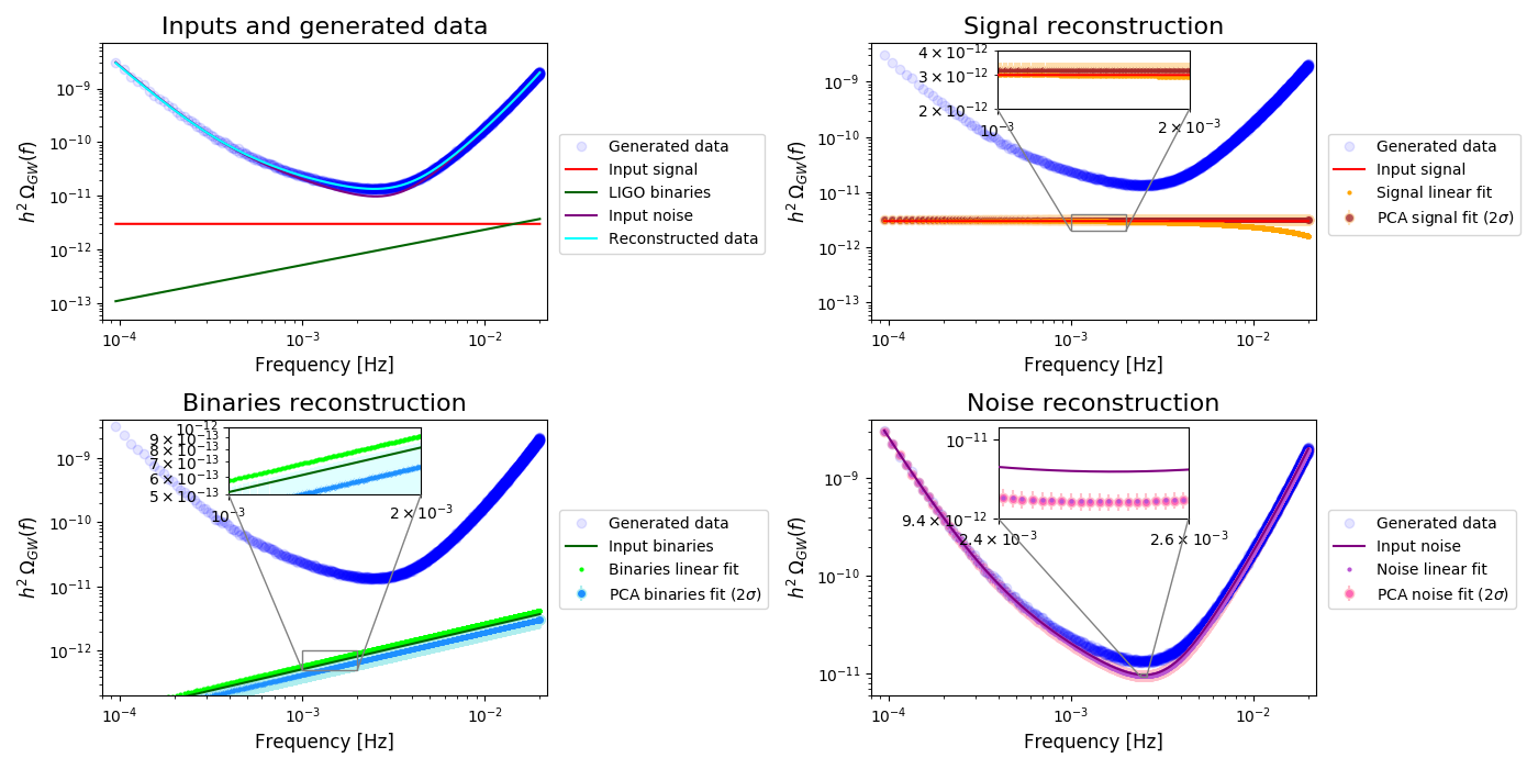
Figure 1: PCA analysis for a flat input signal with amplitude $h^{2}\Omega_{*}=3\times 10^{-12}$ and SNR $\simeq 156$. For this analysis we have fixed $m=10$ and $w=1$Hz (see main text for details). Top left: a plot of all inputs, the simulated data and the reconstructed data. Top right: input signal, linear fit and PCA reconstructions with $2\sigma$ error bands. Bottom left: input LIGO/Virgo foreground (see main text for details), linear fit and PCA reconstructions with $2\sigma$ error bands. Bottom right: input LISA noise (see main text for details), linear fit and PCA reconstructions with $2\sigma$ error bands.

As a first example, we consider in fig. 1 a flat background with amplitude $h^{2}\Omega_{*}=3\times 10^{-12}$, corresponding to SNR $\simeq 156$. Note that in this case the injected signal is larger than the foreground from LIGO/Virgo binaries in most of the frequency range. Moreover, since this signal is constant in the LISA band, it is appropriate to choose a large correlation length $w$, but that causes a large degeneracy between $S_{LV}$ and $S_{\rm signal}$. This makes it numerically difficult to disentangle the two components. An efficient way to resolve this issue is to reduce the dimensionality $m$ of the signal basis In the analysis presented in fig. 1, we choose a basis of $m=10$ Gaussians (with a uniform logarithmic spacing for the pivot frequencies $f^{a}_{i}$) and $w=1$Hz. As can be seen from fig. 1, which shows the PCA reconstructed signal, foreground and noise, this choice very efficiently disentangles the different components hidden in the data. The reconstructed value for the LIGO/Virgo foreground parameter is $L\simeq 1.044\pm 0.114$. As for the LISA noise parameters, we obtain $A\simeq 0.980\pm 0.005$ and $O\simeq 0.976\pm 0.001$. Concerning the reconstruction of the signal, we can see from the top right panel that the linear fit (defined as the model minimizing the $\chi^{2}$ in eq. 17, or equivalently by the sum given in eqs. (26)–(28), where all coefficient are included, irrespectively of their value) correctly reconstructs the signal in most of the frequency range. However, at large frequencies, where the foreground is larger than the signal, it fails. On the other hand the PCA reconstruction, by dropping low information components, produces a fairly accurate reconstruction of the signal even in this range.

In fig. 2, we consider the opposite situation, i.e. we consider an injected signal smaller than the LIGO/Virgo foreground in most of the frequency range. In more detail, we choose a flat signal with amplitude $h^{2}\Omega_{*}=6\times 10^{-13}$, corresponding to an SNR $\simeq 31$. Consistently with the analysis of fig. 1, we have used $w=1$Hz and $m=10$ (with the same uniform logarithmic spacing for the pivot frequencies). We can see that while in this case the reconstruction the LISA noise parameters is basically unaffected ($A\simeq 0.978\pm 0.005$ and $O\simeq 0.975\pm 0.001$), the determination of LIGO/Virgo foreground parameter is slightly more accurate ($L\simeq 0.896\pm 0.106$). As for the signal reconstruction, the top right panel of fig. 2 clearly shows that, despite the signal being much smaller than the LIGO/Virgo foreground, our procedure still captures it in most of the frequency range. Once again the PCA reconstruction works better than a simple linear fit in the region where the signal is much weaker than the foreground.

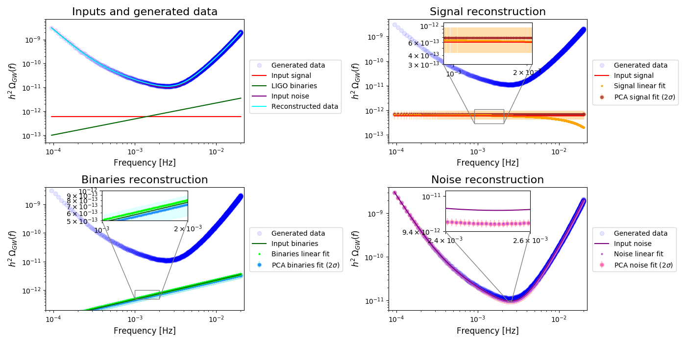
Figure 2: PCA analysis for a flat input signal with amplitude $h^{2}\Omega_{*}=6\times 10^{-13}$ and SNR $\simeq 31$. This analysis was performed with $m=10$ and $w=1$Hz. Plot structure as in fig. 1.

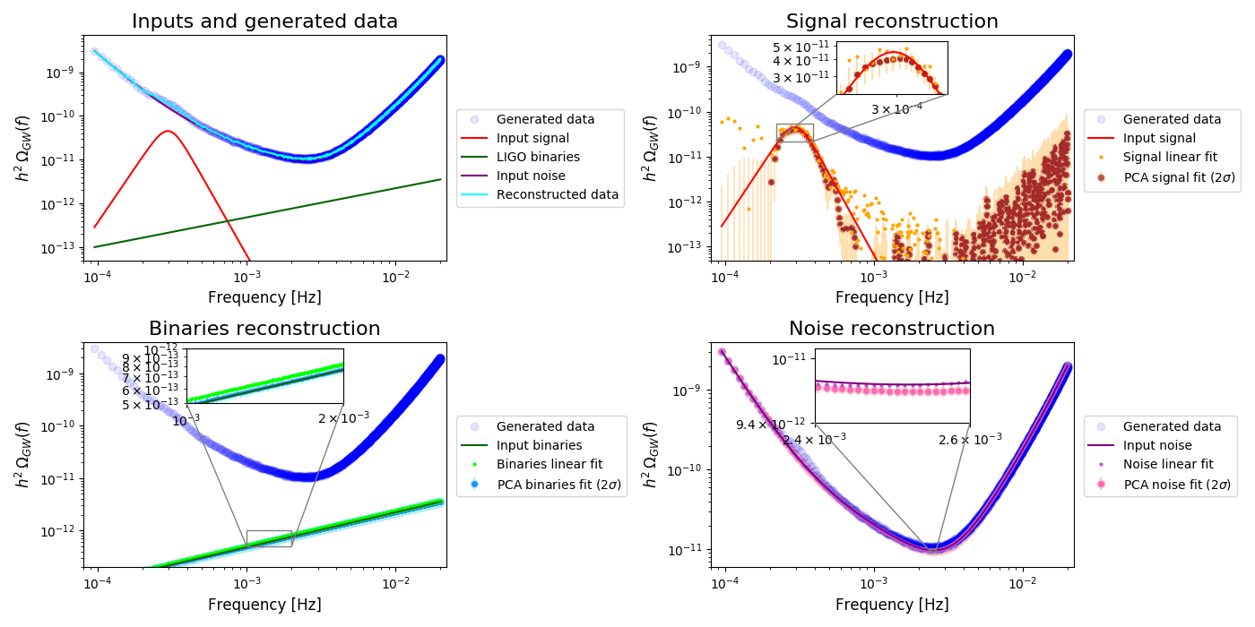
Figure 3: PCA analysis for an input broken power law signal (see footnote 9) with amplitude $h^{2}\Omega_{*}=9\times 10^{-11}$, $n_{s1}=5$, $n_{s2}=-6$ and $f_{*}=3\times 10^{-4}$Hz. The SNR of this signal is $\simeq 34$. This analysis was performed with $m=n$, $w=2\times 10^{-5}$Hz. Plot structure as in fig. 1.

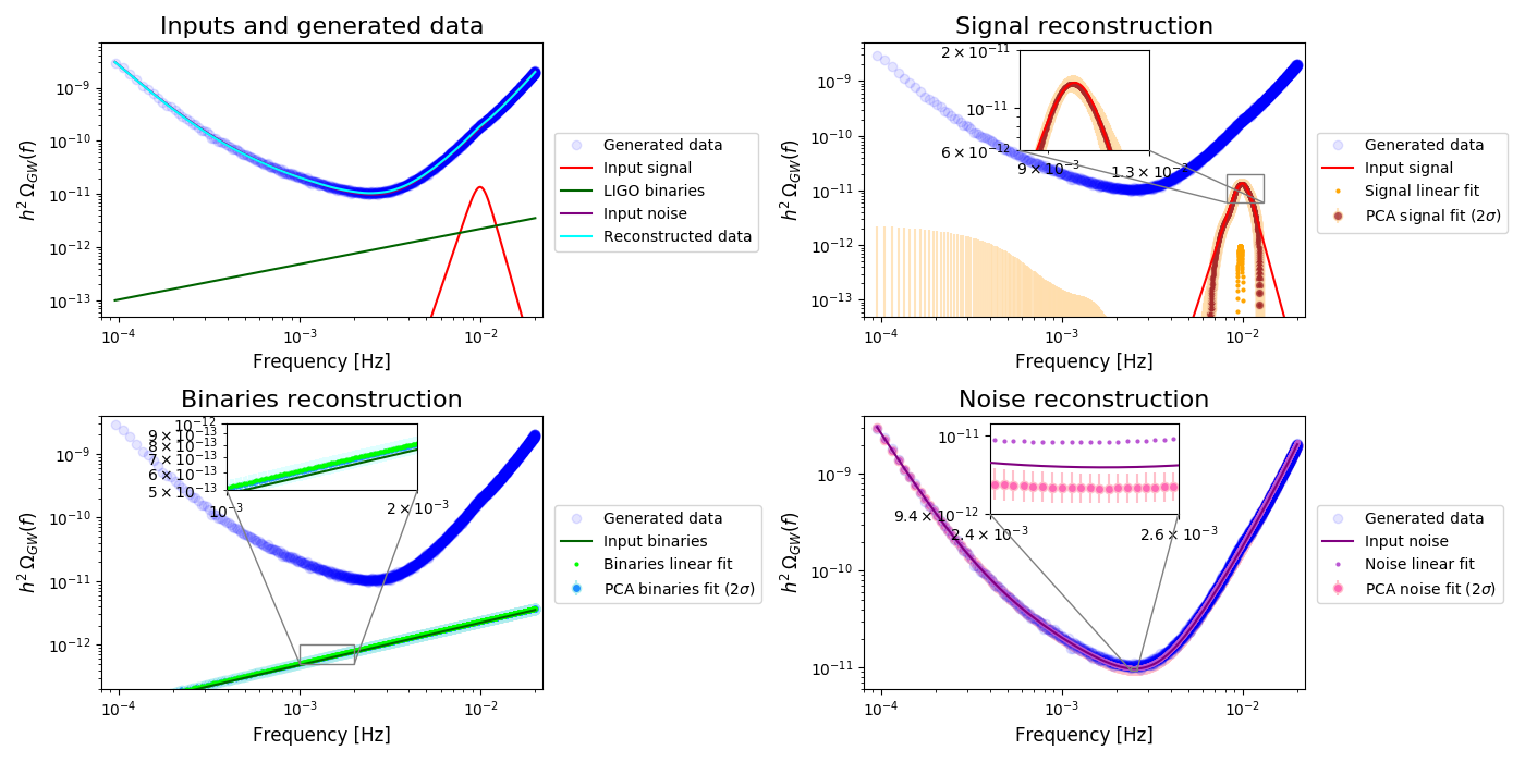
Figure 4: PCA analysis for an input broken power law signal (see footnote 9) with amplitude $h^{2}\Omega_{*}=9\times 2.7\times 10^{-11}$, $n_{s1}=10$, $n_{s2}=-12$ and $f_{*}=10^{-2}$Hz. The SNR of this signal is $\simeq 34$. This analysis was performed with $m=100$ with uniform log spacing and $w=5\times 10^{-4}$Hz. Plot structure as in fig. 1.

We conclude this section by showing two cases where the input signal is chosen to be less degenerate with the foreground. In fig. 3 we show the results obtained by applying our procedure ($m=n$, $w=2\times 10^{-5}$Hz) to a broken power law signal  placed at small frequencies and with SNR $\simeq 34$. In fig. 4 we show instead the results obtained with $m=100$ with uniform log spacing and $w=5\times 10^{-4}$Hz on an injected signal given by a broken power law placed at high frequencies and with SNR $\simeq 34$. In both cases, the reconstruction of the LIGO/Virgo foreground is accurate ($L\simeq 0.948\pm 0.034$ and $L\simeq 0.989\pm 0.045$ respectively), as is the case for the LISA noise parameters ($A\simeq 1.000\pm 0.004$, $A\simeq 0.983\pm 0.009$ and $O\simeq 0.981\pm 0.001$, $O\simeq 0.984\pm 0.002$ respectively).

4 Discussion

In this work we have proposed a template-free PCA technique for the reconstruction of SGWBs with LISA. We have shown that our procedure is very efficient at disentangling an unknown input signal from the instrumental noise even in the presence of a foreground. Remarkably, the component separation obtained with the techniques presented in this work is effective even for signals with fairly small SNR $\simeq 30$, compared to a power-law foreground from LIGO/Virgo binaries with SNR$\simeq 53$.

Our approach essentially consists of expanding the signal onto a basis of Gaussians with fixed width $w$ and centered on a set of pivot frequencies within the LISA frequency band. Generically, an unknown signal can thus be expressed as a linear combination of these functions through some unknown parameters to be determined. We model uncertainties in the LISA noise budget and in the amplitude of the LIGO/Virgo foreground with global normalization parameters also to be determined. The best fit for all these parameters can be then be found by maximizing the posterior distribution given by Bayes’ theorem. By dividing the time series of the data in chunks and using the central limit theorem, we manage to reduce this maximization procedure to a linear problem, which only requires the inversion of the Fisher matrix of the parameters. This inversion can be challenging because of the large dimensionality of the problem, which makes the matrix singular or almost singular (i.e. most combinations of the parameters are essentially unconstrained by the data).

The PCA technique provides in fact a robust technique to tackle this issue, by essentially dropping all the linear combinations of the parameters on which the data provide no information, and retaining only the “components” that are informed by the data. This procedure leads to a “de-noised” agnostic reconstruction of the underlying signal, as well as of the LISA instrumental noise and astrophysical LIGO/Virgo foreground.

In conclusion, the method described in this work is efficient at disentangling the different components of the SGWB that LISA will measure. Our results are of major relevance since they clearly show that foreground subtraction can be successfully performed. This would allow for the identification (and eventually for the characterization) of the possible cosmological signals that might be hidden behind the foreground. Moreover, since our technique is based on a template-free approach, it provides a robust tool applicable to any background signal. Indeed, while in this work we have restricted our analysis to LISA, our techniques can be easily extended to different detectors.

Appendix A The noise and foreground default models

In each of the time-delay interferometry (TDI) channels $X$, $Y$ and $Z$, the LISA experiment will provide data $x(f)$ whose auto-correlation

$$\langle x(f)x^{*}(f^{\prime})\rangle=\frac{1}{2}\delta(f-f^{\prime})\left[\mathcal{R}(f)S_{\rm sign+fg}(f)+P_{\rm noise}(f)\right]$$ (34)

where $\mathcal{R}(f)$ is the detector polarization- and sky-averaged response function, $S_{\rm sign+fg}(f)$ is the strain power spectral density of the signals and foregrounds, while $P_{\rm noise}(f)=P_{\rm acc}(f)+P_{\rm OMS}(f)$ is expected to be comprised of two contributions, one from the single mass acceleration noise and one from the optical metrology system noise. In more detail, these two noise contributions are expected to be given by LISA_docs

$$P_{\rm acc}(f) =16\sin^{2}\left(\frac{2\pi fL}{c}\right)\left[3+\cos^{2}\left(\frac{4\pi fL}{c}\right)\right]\left(3\frac{{\rm fm}}{{\rm s}^{2}\,\sqrt{\rm Hz}}\right)^{2}\times$$ (35)

$$\qquad\times\left[1+\left(\frac{0.4\,\textrm{mHz}}{f}\right)^{2}\right]\left[1+\left(\frac{f}{8\,\textrm{mHz}}\right)^{4}\right]\left(\frac{1}{2\pi f}\right)^{4}\left(\frac{2\pi f}{c}\right)^{2}\;,$$

$$P_{\rm OMS}(f) =16\sin^{2}\left(\frac{2\pi fL}{c}\right)\left(15\frac{{\rm pm}}{\sqrt{\rm Hz}}\right)^{2}\left[1+\left(\frac{2\,\textrm{mHz}}{f}\right)^{4}\right]\left(\frac{2\pi f}{c}\right)^{2}\;,$$

while the response function can be well approximated by Caprini:2019pxz ; LISA_docs

$$\mathcal{R}(f)\simeq 16\sin^{2}\left(\frac{2\pi fL}{c}\right)\frac{3}{10}\frac{1}{1+0.6(2\pi fL/c)^{2}}\left(\frac{2\pi fL}{c}\right)^{2}\,$$ (36)

where $L=2.5$ Gm is the arm length. Note that this simplified noise budget relies on the assumption that the constellation’s arm lengths are equal and constant, and that noise contributions of the same kind present the same power spectral density. As explained in the main text, we account for this uncertainties by introducing two parameters $A$ and $O$ rescaling the amplitudes of the acceleration and optical metrology power spectral densities, with Gaussian priors of about 20% width.

In this paper, rather than working directly with the data $x(f)$, we work with $d(f)\equiv\sqrt{2}x(f)/\sqrt{\mathcal{R}(f)}$, in terms of which eq. 34 becomes

$$\langle d(f)d^{*}(f^{\prime})\rangle=\delta(f-f^{\prime})[S_{\rm sign+fg}(f)+S_{\rm acc}(f)+S_{\rm OMS}(f)]\,,$$ (37)

where we have defined

$$S_{\rm acc}(f)=\frac{P_{\rm acc}(f)}{\mathcal{R}(f)}\,,\qquad\qquad S_{\rm OMS}(f)=\frac{P_{\rm OMS}(f)}{\mathcal{R}(f)}\,.$$ (38)

As in the main text, we can then decompose $S_{\rm sign+fg}(f)$ into signal(s) and foreground(s). For the latter, the contribution from Galactic binaries presents a yearly modulation that is expected to allow for its subtraction, and thus focus only on the background from LIGO/Virgo binaries. At low frequencies, their signal is very well approximated by Regimbau:2011rp ; Maggiore:1900zz ; LIGOScientific:2019vic

$$S_{\rm LV}(f) =\frac{3H_{0}^{2}}{4\pi^{2}f^{3}}\Omega_{\rm GW}(f)\,,$$ (39)

$$\Omega_{\rm GW}(f) =\Omega_{*}\left(\frac{f}{f_{*}}\right)^{2/3}\,,$$ (40)

where $H_{0}=h\,100{\rm km/(sMpc)}$, $h=0.679$ Aghanim:2018eyx , and $\Omega_{*}$ – i.e. the amplitude at the pivot frequency $f_{*}=25$ Hz – will be measured by LIGO/Virgo at design sensitivity ligostoch ; Martynov:2016fzi . As our default value, we assume here $\Omega_{*}=8.9\times 10^{-10}$, which is the current best estimate based on the measured rate of coalescence of resolved neutron star and stellar origin black hole binaries in LIGO/Virgo LIGOScientific:2019vic . As mentioned in the main text, to show the robustness of our methods we use a conservative estimate of $\sigma_{L}=0.5$ for the width of our prior in eq. 15.

Finally, we recall that the SNR of a SGWB can be computed as

$${\rm SNR}\equiv\sqrt{T\int_{f_{\text{min}}}^{f_{\text{max}}}df\,\left(\frac{S_{h}(f)}{S_{n}(f)}\right)^{2}}\,,$$ (41)

where $f_{\text{min}}$, $f_{\text{max}}$ are respectively the minimum and maximum frequencies to which the detector is sensitive, $T$ is the observation time (which we set in this paper to 4 yr with $75\%$ efficiency), and $S_{h}$ and $S_{n}$ are respectively the SGWB and detector noise power spectral densities.

Appendix B Downsampling the data

In this Appendix, we provide additional details on our downsampling procedure. As mentioned in the main text, let us start by bundling the data in groups of $M$ points adjacent in frequency. If the frequency range spanned by these $M$ data is sufficiently small, we can locally approximate the power spectral density within this range by performing a linear fit. To this purpose, it is convenient to introduce the reference frequency $\bar{f}\equiv(\sum_{i}f_{i}/S_{i}^{2})/(\sum_{i}1/S_{i}^{2})$ (where the index $i$ spans the $M$ points under consideration), express the data in terms of the distance from this reference frequency, i.e. $\delta f=f-\bar{f}$, and fit the data with $S=a\delta f+b$.

By assuming uniform priors on $a$ and $b$, and using the fact that the data are independent Gaussian variables if eq. (6) is valid, Bayes’ theorem returns the same answer as the standard $\chi^{2}$ fit procedure, i.e. the best estimates for $a$ and $b$ are DAbook

$$a=\frac{\beta p-\gamma q}{\alpha\beta-\gamma^{2}}\,,\quad b=\frac{\alpha q-\gamma p}{\alpha\beta-\gamma^{2}}$$ (42)

$$\alpha=\sum_{i}\omega_{i}\delta f_{i}^{2}\,,\quad\beta=\sum_{i}\omega_{i}\,,\quad\gamma=\sum_{i}\omega_{i}\delta f_{i}\,\quad p=\sum_{i}\omega_{i}\delta f_{i}\bar{D}_{i}\,,\quad q=\sum_{i}\omega_{i}\bar{D}_{i}\,,$$ (43)

where the weights $\omega_{i}=2/\sigma_{i}^{2}$ depend on the errors of the data, $\sigma_{i}=S_{i}/\sqrt{N}$. Note that from the definition of the $\delta f_{i}$ as distances from the reference frequency $\bar{f}$, it follows that $\gamma=0$. The best estimate for $b=S(f=\bar{f})\equiv\bar{S}$ is therefore $b={q}/{\beta}$, which coincides with the weighted average of the data, $\bar{\bar{D}}$, defined in the main text.

Moreover, the posterior distribution for the parameters $a$ and $b$ is a Gaussian with covariance matrix DAbook

$$\sigma^{2}_{aa} =\frac{2\beta}{\alpha\beta-\gamma^{2}}\,,$$ (44)

$$\sigma^{2}_{bb} =\frac{2\alpha}{\alpha\beta-\gamma^{2}}\,,$$ (45)

$$\sigma^{2}_{ab} =\sigma^{2}_{ba}=-\frac{2\gamma}{\alpha\beta-\gamma^{2}}\,.$$ (46)

Since $\gamma=0$ in our case, $b$ is uncorrelated from $a$ and its posterior distribution is Gaussian with variance $\sigma^{2}_{bb}=2/\beta$. This means that the (Gaussian) variance to be ascribed to $\bar{\bar{D}}$ is $(\sum_{i}1/\sigma^{2}_{i})^{-1}=N^{-1}(\sum_{i}1/S^{2}_{i})^{-1}$, which we can approximate by $\bar{S}^{2}/(NM)$ if the $S_{i}$ do not vary strongly.

References

- (1) LISA collaboration, Laser Interferometer Space Antenna, 1702.00786.
- (2) LIGO Scientific collaboration, Advanced LIGO, Class. Quant. Grav. 32 (2015) 074001 [1411.4547].
- (3) F. A. et al, Advanced Virgo: a second-generation interferometric gravitational wave detector, Class. Quant. Grav. 32 (2015) 024001.
- (4) S. Hild et al., Sensitivity Studies for Third-Generation Gravitational Wave Observatories, Class. Quant. Grav. 28 (2011) 094013 [1012.0908].
- (5) A. Sesana, F. Haardt, P. Madau and M. Volonteri, Low-Frequency Gravitational Radiation from Coalescing Massive Black Hole Binaries in Hierarchical Cosmologies, Astrophys. J. 611 (2004) 623 [astro-ph/0401543].
- (6) A. Sesana, F. Haardt, P. Madau and M. Volonteri, The Gravitational Wave Signal from Massive Black Hole Binaries and Its Contribution to the LISA Data Stream, Astrophys. J. 623 (2005) 23 [astro-ph/0409255].
- (7) E. Barausse, The evolution of massive black holes and their spins in their galactic hosts, Mon. Not. R. Astron. Soc. 423 (2012) 2533 [1201.5888].
- (8) A. Klein et al., Science with the space-based interferometer eLISA: Supermassive black hole binaries, Phys. Rev. D 93 (2016) 024003 [1511.05581].
- (9) M. Bonetti, A. Sesana, F. Haardt, E. Barausse and M. Colpi, Post-Newtonian evolution of massive black hole triplets in galactic nuclei - IV. Implications for LISA, Mon. Not. R. Astron. Soc. 486 (2019) 4044 [1812.01011].
- (10) S. Babak, J. Gair, A. Sesana, E. Barausse, C. F. Sopuerta, C. P. L. Berry et al., Science with the space-based interferometer LISA. V. Extreme mass-ratio inspirals, Phys. Rev. D 95 (2017) 103012 [1703.09722].
- (11) T. Kupfer, V. Korol, S. Shah, G. Nelemans, T. Marsh, G. Ramsay et al., LISA verification binaries with updated distances from Gaia Data Release 2, Mon. Not. Roy. Astron. Soc. 480 (2018) 302 [1805.00482].
- (12) G. Nelemans, L. R. Yungelson and S. F. Portegies Zwart, Short-period AM CVn systems as optical, X-ray and gravitational-wave sources, Mon. Not. R. Astron. Soc. 349 (2004) 181 [astro-ph/0312193].
- (13) A. J. Ruiter, K. Belczynski, M. Benacquista, S. L. Larson and G. Williams, The LISA Gravitational Wave Foreground: A Study of Double White Dwarfs, Astrophys. J. 717 (2010) 1006 [0705.3272].
- (14) T. R. Marsh, Double white dwarfs and LISA, Classical and Quantum Gravity 28 (2011) 094019.
- (15) V. Korol, E. M. Rossi, P. J. Groot, G. Nelemans, S. Toonen and A. G. Brown, Prospects for detection of detached double white dwarf binaries with Gaia, LSST and LISA, Mon. Not. Roy. Astron. Soc. 470 (2017) 1894 [1703.02555].
- (16) V. Korol, E. M. Rossi and E. Barausse, A multimessenger study of the Milky Way’s stellar disc and bulge with LISA, Gaia, and LSST, Mon. Not. Roy. Astron. Soc. 483 (2019) 5518 [1806.03306].
- (17) S. E. Timpano, L. J. Rubbo and N. J. Cornish, Characterizing the galactic gravitational wave background with LISA, Phys. Rev. D 73 (2006) 122001 [gr-qc/0504071].
- (18) M. R. Adams and N. J. Cornish, Detecting a Stochastic Gravitational Wave Background in the presence of a Galactic Foreground and Instrument Noise, Phys. Rev. D89 (2014) 022001 [1307.4116].
- (19) Virgo, LIGO Scientific collaboration, Observation of Gravitational Waves from a Binary Black Hole Merger, Phys. Rev. Lett. 116 (2016) 061102 [1602.03837].
- (20) A. Sesana, Multi-band gravitational wave astronomy: science with joint space- and ground-based observations of black hole binaries, J. Phys. Conf. Ser. 840 (2017) 012018 [1702.04356].
- (21) K. W. Wong, E. D. Kovetz, C. Cutler and E. Berti, Expanding the LISA Horizon from the Ground, Phys. Rev. Lett. 121 (2018) 251102 [1808.08247].
- (22) D. Gerosa, S. Ma, K. W. Wong, E. Berti, R. O’Shaughnessy, Y. Chen et al., Multiband gravitational-wave event rates and stellar physics, Phys. Rev. D 99 (2019) 103004 [1902.00021].
- (23) A. Nishizawa, A. Sesana, E. Berti and A. Klein, Constraining stellar binary black hole formation scenarios with eLISA eccentricity measurements, Mon. Not. Roy. Astron. Soc. 465 (2017) 4375 [1606.09295].
- (24) A. Nishizawa, E. Berti, A. Klein and A. Sesana, eLISA eccentricity measurements as tracers of binary black hole formation, Phys. Rev. D 94 (2016) 064020 [1605.01341].
- (25) N. Tamanini, A. Klein, C. Bonvin, E. Barausse and C. Caprini, The peculiar acceleration of stellar-origin black hole binaries: measurement and biases with LISA, 1907.02018.
- (26) E. Barausse, N. Yunes and K. Chamberlain, Theory-Agnostic Constraints on Black-Hole Dipole Radiation with Multiband Gravitational-Wave Astrophysics, Phys. Rev. Lett. 116 (2016) 241104 [1603.04075].
- (27) Z. Carson and K. Yagi, Multi-band gravitational wave tests of general relativity, Class. Quant. Grav. 37 (2020) 02LT01 [1905.13155].
- (28) G. Gnocchi, A. Maselli, T. Abdelsalhin, N. Giacobbo and M. Mapelli, Bounding Alternative Theories of Gravity with Multi-Band GW Observations, 1905.13460.
- (29) A. Caputo, L. Sberna, A. Toubiana, S. Babak, E. Barausse, S. Marsat et al., Gravitational-wave detection and parameter estimation for accreting black-hole binaries and their electromagnetic counterpart, 2001.03620.
- (30) LIGO Scientific, Virgo collaboration, Search for the isotropic stochastic background using data from Advanced LIGO’s second observing run, Phys. Rev. D100 (2019) 061101 [1903.02886].
- (31) R. Brito, S. Ghosh, E. Barausse, E. Berti, V. Cardoso, I. Dvorkin et al., Stochastic and resolvable gravitational waves from ultralight bosons, Phys. Rev. Lett. 119 (2017) 131101 [1706.05097].
- (32) R. Brito, S. Ghosh, E. Barausse, E. Berti, V. Cardoso, I. Dvorkin et al., Gravitational wave searches for ultralight bosons with LIGO and LISA, Phys. Rev. D 96 (2017) 064050 [1706.06311].
- (33) E. Barausse, R. Brito, V. Cardoso, I. Dvorkin and P. Pani, The stochastic gravitational-wave background in the absence of horizons, Class. Quant. Grav. 35 (2018) 20LT01 [1805.08229].
- (34) C. Caprini et al., Detecting gravitational waves from cosmological phase transitions with LISA: an update, JCAP 03 (2020) 024 [1910.13125].
- (35) P. Auclair et al., Probing the gravitational wave background from cosmic strings with LISA, 1909.00819.
- (36) N. Bartolo et al., Science with the space-based interferometer LISA. IV: Probing inflation with gravitational waves, JCAP 12 (2016) 026 [1610.06481].
- (37) C. Caprini and D. G. Figueroa, Cosmological Backgrounds of Gravitational Waves, Class. Quant. Grav. 35 (2018) 163001 [1801.04268].
- (38) N. Karnesis, A. Petiteau and M. Lilley, A template-free approach for detecting a gravitational wave stochastic background with LISA, 1906.09027.
- (39) C. Caprini, D. G. Figueroa, R. Flauger, G. Nardini, M. Peloso, M. Pieroni et al., Reconstructing the spectral shape of a stochastic gravitational wave background with LISA, JCAP 1911 (2019) 017 [1906.09244].
- (40) Y. B. Ginat, V. Desjacques, R. Reischke and H. B. Perets, The Probability Distribution of Astrophysical Gravitational-Wave Background Fluctuations, 1910.04587.
- (41) M. Maggiore, Gravitational Waves. Vol. 1: Theory and Experiments, Oxford Master Series in Physics. Oxford University Press, 2007.
- (42) https://www.cosmos.esa.int/web/lisa/lisa-documents.
- (43) LIGO Scientific, Virgo collaboration, GW150914: Implications for the stochastic gravitational wave background from binary black holes, Phys. Rev. Lett. 116 (2016) 131102 [1602.03847].
- (44) B. P. Abbott et al., Sensitivity of the Advanced LIGO detectors at the beginning of gravitational wave astronomy, Phys. Rev. D 93 (2016) 112004 [1604.00439].
- (45) M. Punturo et al., The Einstein Telescope: A third-generation gravitational wave observatory, Class. Quant. Grav. 27 (2010) 194002.
- (46) B. Sathyaprakash et al., Scientific Objectives of Einstein Telescope, Class. Quant. Grav. 29 (2012) 124013 [1206.0331].
- (47) M. Maggiore et al., Science Case for the Einstein Telescope, 1912.02622.
- (48) D. Sivia and J. Skilling, Data Analysis: A Bayesian Tutorial. Oxford University Press, 2006.
- (49) H. Akaike, A new look at the statistical model identification, IEEE Transactions on Automatic Control 19 (6) (1974) 716.
- (50) T. Regimbau, The astrophysical gravitational wave stochastic background, Res. Astron. Astrophys. 11 (2011) 369 [1101.2762].
- (51) Planck collaboration, Planck 2018 results. VI. Cosmological parameters, 1807.06209.