Dynamical Network Models of the Turbulent Cascade

Abstract

Cascade models based on dynamical complex networks are proposed as models of turbulent energy cascade. Taking a simple shell model as the initial regular lattice with only nearest neighbor interactions, small world network models are constructed by adding or replacing some of the existing local interactions by nonlocal ones. The models are then evolved over time, both by solving for the shell variable for velocity using an arbitrary network generalization of the shell model evolution and by rewiring the network each time from the original lattice in regular time intervals. This results in a more intermittent time evolution with larger variations of the wave-number spectrum. It also results in an actual increase in intermittency as computed from the fitted exponents of structure functions as computed from these models. It appears that the intermittency increases as the ratio of random nonlocal connections to local nearest neighbor connections increases.

I Introduction

Turbulence is a duality of chaotic disorder and hierarchical organization across a large range of scales in the evolution of a fluid. This aspect of turbulence is shared with many other self-organizing complex systems, that are commonly described using networks, such as the internet(Albert, Jeong, and Barabási, 1999), the brain(Bullmore and Sporns, 2009), the public transport infrastructure(Seaton and Hackett, 2004), and the economy(Kirman, 1997) - to give a few examples.

The three dimensional incompressible fluid, described by the Navier-Stokes equation, mixed at large scales by an external forcing and dissipated at small scales due to molecular viscosity, provide the canonical example of the turbulent cascade. The idealized process of self-similar energy transfer from large scales where the energy is injected to small scales, where it is dissipated can be described using various simplified models including shell models(Biferale, 2003), differential approximations(Leith, 1967) or closures(Lesieur, 1997). While the study of turbulence has a long history(Frisch, 1995), and networks are ubiquitous in modern nonlinear science(Barabasi, 2011), the connection between the two is an emerging field with many open questions(Taira, Nair, and Brunton, 2016; Gürcan, Li, and Morel, 2020).

Network theory is as much about spreading or flow of various constituents such as information, ideas or pathogens within a given (or evolving) network structure, as it is about the topology of the network itself. Flow of packages through the internet, people through the public transport system(Lee et al., 2008), or the spreading of financial crises through the global economy(KALI and REYES, 2010) or a deadly virus across a network of human contacts(Keeling and Eames, 2005) are all examples of such phenomena that fall under the umbrella term of percolation in complex networks(Dorogovtsev, Goltsev, and Mendes, 2008; Watts, 2002). The turbulent cascade of energy in a complex network representing the wavenumber domain, fits right in with the rest of these examples. However there is a key difference in the turbulent problem: the interactions are between three nodes instead of two, since they are produced by triadic interactions. In this sense the turbulent cascade takes place one a network with “three body” interactions(Neuhäuser, Mellor, and Lambiotte, 2020).

In this spirit, we propose a concrete working example in the form of a model of the turbulent cascade using dynamical complex networks by generalizing the GOY model(Ohkitani and Yamada, 1989) to a percolation model on a complex, small world network with long range interactions. This allows the exploration of different strategies of random rewiring of a regular lattice in order to form nontrivial small-world networks(Newman, 2003) on which the turbulence is then allowed to develop. Two different rewiring strategies based on Watts-Strogatz and Newman-Watts are discussed and dynamical network models are considered where the network is regularly rewired. Energy cascade is described on top of this evolving small world network using a simple shell model-like evolution of the observables $u_{n}\left(t\right)\equiv\sqrt{2\int_{k_{n}}^{k_{n+1}}E\left(k\right)dk}$. While this would probably appear quite unphysical to a specialist in turbulence, since the turbulence can be described nicely on a constant regular grid with deterministic equations, its power comes from the additional degree of freedom -i.e. that of the network topology- that it provides, which allows us to represent part of what has been lost in the reduction leading up to the shell model at a very modest cost -the solution of the network model is not slower than the GOY model-.

Shell models are closely linked to the concept of spectral reduction(Bowman, Shadwick, and Morrison, 1999), which basically amounts to reducing the regular spectral domain to a smaller set of regions. When the full spectral domain is thus reduced, detailed phase relations between regions are lost. The shell model does have a complex phase that evolves, but this has almost nothing to do with the actual phase of the full system. The direction of energy transfer at a given instant, or its efficiency depends on these phase relations. If the phases are aligned between two regions, the energy can be transferred efficiently, while if they are out of phase, there may be no energy transfer. While the evolution of phases is deterministic in the full system, its chaotic and usually irregular. Therefore its effect on a shell model like reduction can be represented plausibly by connections being turned on and off randomly. Note that on top of the connection being turned on the phase relations of the shell model itself still has to be satisfied for the energy transfer to take place. For a real physical problem, phase relations may be random or regular, for instance as in the case of weak wave turbulence(Newell and Rumpf, 2011). In such a case, the network topology may be constructed respecting the dispersion relation of the underlying waves, and the network may be used to represent those ’enhanced’ connections between disparate scales due to resonant interactions. If the statistics of those phenomena are well represented by the evolution of the network, its time evolution may correspond better to the time evolution of the unreduced system.

The rest of the paper is organized as follows. In section II we introduce the basic small world network paradigm for turbulence using a generalization of the GOY model. In sections II.1 and II.2 we lay out the strategies for constructing Watts-Strogatz and Newman-Watts models respectively, while in II.3 we discuss the bipartite network perspective using two sets of nodes corresponding to wavenumbers and triads. In section III we provide the numerical results of all these different models compared to the basic GOY model. Section IV is conclusion.

II Small World Network Shell Models

Consider a shell model of turbulence (Biferale, 2003) with arbitrary range interactions for three dimensional turbulence. Using a set of wave-vectors $k_{n}=k_{0}g^{n}$, where $g$ is the logarithmic scaling factor (usually $g=2$), the model can be written as follows:

$$\partial_{t}u_{n}=i\alpha_{m}\bigg{[} a_{n}^{m}u_{n+m}^{*}u_{n+m+1}^{*}+b_{n}^{m}u_{n+1}^{*}u_{n-m}^{*}$$

$$+c_{n}^{m}u_{n-1}^{*}u_{n-1-m}^{*}\bigg{]}$$ (1)

where the interaction coefficients can be written as $a_{n}^{m}=M_{n,n+m,n+m+1}$, $b_{n}^{m}=M_{n,n-m,n+1}$ and $c_{n}^{m}=M_{n,n-1-m,n-1}$ with:

$$M_{n,\ell,\ell^{\prime}}=\begin{cases}k_{\ell}+k_{\ell^{\prime}}&\text{if }n<\ell\\ -\left(\left(-1\right)^{n-\ell}k_{\ell}+k_{\ell^{\prime}}\right)&\text{if }\text{$\ell<n$}\end{cases}$$ (2)

Here $m$ is the range of interaction (i.e. $m=1$ gives us the usual GOY model), and $\alpha_{m}$ is the average contribution from the geometric factor, which we take as $\alpha_{m}=g^{-m}$ (see for example (Plunian and Stepanov, 2007)). Note that $\ell<\ell^{\prime}$ is assumed in (2). This allows conservation of energy

$$E=\sum_{n}u_{n}^{2}$$

and helicity

$$H=\sum_{n}\left(-1\right)^{n}k_{n}^{-1}u_{n}\;\text{,}$$

since

$$M_{n,n+m,n+m+1}+M_{n+m,n,n+m+1}+M_{n+m+1,n,n+m}=0$$

and

$$k_{n}M_{n,n+m,n+m+1}+\left(-1\right)^{m}k_{n+m}M_{n+m,n,n+m+1}$$

$$+\left(-1\right)^{m+1}k_{n+m+1}M_{n+m+1,n,n+m} =0\;\text{.}$$

Figure 1: The regular lattice of the GOY model. Apart from the end nodes, all the nodes are connected to three triads and each triad is connected to the three closest nodes. The lattice is shown in a circular representation in order to save space and connect to earlier works.

The three terms in (1) come from the three triadic interactions that have the same form but shifted with respect to one another. The first term proportional to $a_{n}^{m}$ describes the interaction between the shells $n$, $n+m$ and $n+m+1$. The last two terms proportional to $b_{n}^{m}$ and $c_{n}^{m}$ are the same interaction but shifted by $-m$ and $-m-1$ respectively. This allows us to consider different terms in the equation in terms of undirected triadic interactions. For example a single triadic connection $\left(n,n+m,n+m+1\right)=\left(1,4,5\right)$ introduces one term in the equation for $u_{1}$ with the coefficient $a_{1}^{3}=M_{145}$, one term in the equation for $u_{4}$ with the coefficient $b_{4}^{3}=M_{415}$ and finally one term in the equation for $u_{5}$ with the coefficient $c_{5}^{3}=M_{514}$.

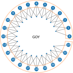
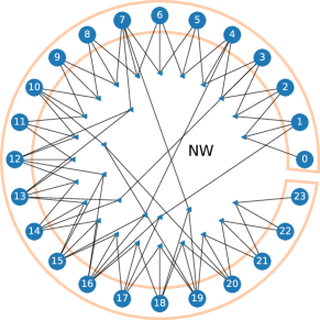
The standard GOY model corresponds to $m=1$, which represents “nearest neighbor” interactions shown in figure 1. If we choose $g=2$, and absorb a prefactor $6$ into the arbitrary constant $\alpha$, (2) gives $a_{n}=k_{n}$, $b_{n}=-k_{n-1}/2$ and $c_{n}=-k_{n-2}/2$ of Ref. Ohkitani and Yamada, 1989.

Figure 2: Wave number spectrum for the WS network, generated with $p=0.4$, $p_{f}=0.5$, compared with the GOY model shown with thick orange (if in color) line. Nodes $5$, $9$, $10$, $12$ and $13$ are missing connections which results in formation of peaks or wells. The fact that energy can go to dissipative range through non-local connections makes the spectrum fall off rapidly at around $10^{4}$. Here $N=24$, $k_{0}=2^{-4}$, $\nu=10^{-8}$ and $f_{n}=\left(\delta_{n1}\xi_{1}+\delta_{n2}\xi_{2}\right)10^{-2}$, where $\xi_{i}$ are random variables with a correlation time of $10^{-2}$. The spectra are integrated up to $t=5\times 10^{3}$ and average over $t=\left[3-5\right]\times 10^{3}$ are shown.

II.1 Watts-Strogatz model

There is a total of $N-2$ triads in the regular lattice of the GOY model with $N$ nodes. In order to create a partially randomized network with non-local interactions, we go over this list of triads and replace the local triad $\left(n,n+1,n+2\right)$ with a nonlocal one, with either a forward, [i.e. $\left(n,n+m,n+m+1\right)$] or a backward [i.e. $\left(n,n-m,n-1\right)$] coupling with a probability $p$, where $m$ itself is a random number between $2$ and $N-n-2$ for the forward or between $3$ and $n-2$ for the backward coupling. We can choose the interaction to be forward with a probability $p_{f}$. This basic algorithm is very similar to the one described by Watts and Strogatz in order to build small world networks(Watts and Strogatz, 1998) (so we call it the Watts-Strogatz model or WS for short), except that the topology of the initial lattice is not really a ring, and the connections are not lines, but triadic interactions.

Having the list of triads thus revised, we can recompute the list of interactions $\mathbf{i}_{n}=\left\{\ell^{\prime},\ell^{\prime\prime}\right\}$ and the interaction coefficients (i.e. weights) $M_{n,\ell,\ell^{\prime}}$ for each node using the triads that connect to it. The idea is to go over the list of triads, and for example when treating the triad $\left(n,n+m,n+m+1\right)$, add the three interactions $\mathbf{i}_{n}=\left\{n+m,n+m+1\right\}$, $\mathbf{i}_{n+m}=\left\{n,n+m+1\right\}$ and $\mathbf{i}_{n+m+1}=\left\{n,n+m\right\}$ to the list of interactions, with the corresponding interaction coefficients $M_{n,n+m,n+m+1}$, $M_{n+m,n,n+m+1}$ and $M_{n+m+1,n,n+m}$ respectively. In the end, one may have nodes with more or less connections than three (the original number of connections of each node in the GOY model), and these connections may be local or nonlocal, but since the contributions from each triad to all its three nodes are always considered, the conservation laws are automatically respected. The model goes from the regular shell model with local interactions for $p=0$ to a cascade model with random scale interactions for $p=1$. In contrast, $p_{f}$ does not play an important role on network topology, so one could pick all the connections to be forward without loss of generality.

Figure 3: The small world network of the WS model, generated with $p=0.4$,$p_{f}=0.5$ also shown in Figure 2 with less than three connections at nodes $5$, $9$, $10$, $12$ and $13$.

Once the network is constructed, time evolution of the node variables $u_{n}$ can be written as:

$$\left(\partial_{t}+\nu k_{n}^{2}\right)u_{n} =\sum_{\ell^{\prime},\ell^{\prime\prime}=\mathbf{i}_{n}}M_{n,\ell,\ell^{\prime}}u_{\ell}^{*}u_{\ell^{\prime}}^{*}\;+f_{n}\text{,}$$ (3)

where $\mathbf{i}_{n}$ is the list of interaction pairs for the $n$th node, and $M_{n,\ell,\ell^{\prime}}$ are the interaction coefficients, $\nu$ is kinematic viscosity and $f_{n}$ is (localized and random) forcing.

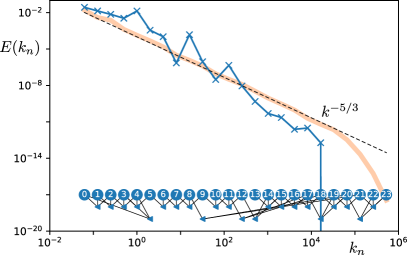
A static network that is integrated for a certain number of time steps is not a particularly interesting exercise. In particular since the result relies on initialization and how the network is wired. The resulting spectrum is a considerably rugged version of the shell model one, as seen in fig. 2, with barriers around nodes that are missing connections. Furthermore each time the network is rewired, the details of how it deviates from the regular shell model would change. Figure 3 shows the particular wiring in more detail that leads to the spectrum shown in figure 2. Notice that some nodes are missing connections, and the energy has difficulty going through those.

A more realistic approach is to rewire the network in regular time intervals (i.e. $\Delta t$) as the system evolves. If we run such a model for a long enough time $t\gg\Delta t$ we can obtain good statistics. Various interesting problems related to shell models, such as intermittency etc. can also be studied in this formulation. Note that in order to not completely randomize the network in a few time steps, we apply the WS strategy on the original network and not the modified one at $t$ in order to obtain the network structure at $t+\Delta t$. The results for this dynamical network formulation using the WS strategy can be seen in section III along with results for the other strategies.

II.2 Newman-Watts model

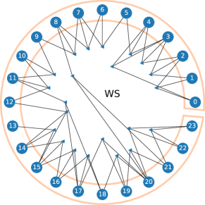
Newman and Watts proposed an alternative algorithm for constructing a similar partially randomized network from a regular initial lattice(Newman and Watts, 1999). It translates to shell models as adding a non-local triad instead of replacing the local one as in WS, with, $m$, $p$ and $p_{f}$ having the same roles as before. We call this, the Newman-Watts strategy or NW for short. The steady-state wave-number spectrum on a network obtained by this algorithm is shown in figure 4, where the network itself is shown in figure 5. Note that since the algorithm simply adds connections and the interaction coefficients for those nonlocal connections go down as $g^{-m}$, the result is very similar to GOY.

Figure 4: Wave number spectrum for the NW network, generated with $p=0.4$, $p_{f}=1.0$ compared with the GOY model. All the nodes have at least $3$ connections therefore no barriers appear. Also the additional connections dissipative range make the spectrum fall off a bit faster. Parameters and run times are the same as in figure 2.

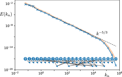
The primary advantage of the NW is that it keeps the basic structure of the underlying regular local lattice. This allows the basic local transfers to always be present, giving a smoother steady state spectrum. In any case, the more relevant formulation of the model is not a single network instance but a dynamically rewired one, whose results are shown below in section III.

Figure 5: The small world network of the NW model, generated with $p=0.4$, $p_{f}=1.0$, which is the same network as the one in Figure 4.

II.3 Bipartite Networks of Wave-numbers and Triads for Describing Turbulence

The discussion of dynamical complex network models above is based on interactions between nodes and pairs, where each interaction is represented by a triad, and we talk about nodes that are connected to triads. The graphs of networks in figures 1,3 and 5 show these triads explicitly. This is actually a hint at the underlying nature of networks that appear in spectral description of turbulence. These networks with three body interactions can also be represented as bipartite networks(Vasques Filho and O’Neale, 2018) that exclusively connect two separate kinds of nodes “wave-number nodes” representing wave-number domains and “triad nodes” representing triadic interactions, with the additional constraint that each triad has three connections. This perspective allows us to transform networks where nodes are connected to pairs, into the simpler and well known class of bipartite networks, and to ask common questions in network topology such as average distance, clustering coefficients or degree distributions. In particular, using the bipartite network but focusing on the wave-number nodes, we can construct a projected simple (or multi or weighted) graph network as discussed in Ref. Vasques Filho and O’Neale, 2018, where the nodes in the projected network are connected only if they are both connected to the same triad.

Figure 6: The resulting steady state spectra from the dynamical complex network models WS and NW compared with that of the GOY model, showing that all three models basically capture the $k^{-5/3}$ spectrum that we expect, while NW is very slightly lower in amplitude as opposed to the other two probably as a result of its extra connections, and therefore higher transfer efficiency. The parameters for these runs are discussed in the text.

III Numerical Results

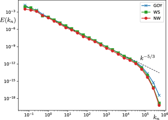
Here we focus on the results from the dynamical network models discussed above, which are rewired according to either WS or NW in regular intervals of $\Delta t$. Unlike the static cases, there is no big difference between the two in terms of their steady state spectra as shown in figure 6, since an evolving network moves its barriers around, and as a result, allows energy transfer, more easily. The results shown in this section uses the parameters $N=24$, $k_{0}=2^{-4}$, $\nu=10^{-8}$ and $f_{n}=\left(\delta_{n1}\xi_{1}+\delta_{n2}\xi_{2}\right)10^{-2}$, where $\xi_{i}$ are random variables with a correlation time of $10^{-2}$. The spectra are integrated up to $t=5\times 10^{3}$ using an adaptive fourth order Runge Kutta solver(Gürcan, 2020), and when steady state results are shown they are usually averaged over $t=\left[3-5\right]\times 10^{3}$.

2.

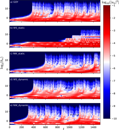
The initial phase of the time evolution for different models can be seen in Figure 7. Here, the nodes with less than three connections act as barriers in the static WS case. This results in a slower buildup and a very noisy final spectrum as shown in figure 2. In contrast, in the static NW case, non-local connections weaken the initial broadening of the energy spectrum around the production region by coupling directly to small scales that are strongly dissipative. This results in a slower buildup as well. However since there are no barriers in NW, the final state is roughly the same with that of GOY. In contrast, since the network evolution time scale $\Delta t=10^{-2}$ is much faster compared to the time it requires to reach steady state, evolving network acts as a halo connecting all the nodes to one another, speeding up the redistribution of energy. Changing $\Delta t$ has a nontrivial impact on the dynamics of WS, but not so for NW. Since WS has barriers, how long those stay in one place affects the dynamics. We don’t show a $\Delta t$ scan here explicitly, but this can be seen from the difference between the static (i.e. $\Delta t\rightarrow\infty$) vs. dynamic network versions of the WS shown in figure 7.

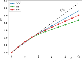
Another interesting tool in understanding the dynamics of the turbulent cascade is the structure function, which gives information about the scale by scale distribution of statistical features of the flow field. The shell model equivalent of the $\ell$th order structure function can be written as $S_{\ell}^{n}=\left\langle\left|u_{n}\right|^{\ell}\right\rangle$ where the average is to be computed over time. Assuming that it has a power law form: $S_{\ell}^{n}\propto k_{n}^{-\xi_{\ell}}$, one can obtain $\xi_{\ell}$ by considering $y_{\ell}=\log_{10}\left(S_{\ell}^{n}\right)$, and $x=\log_{10}\left(k_{n}\right)$ and making a linear regression to obtain $y_{\ell}=a_{\ell}+b_{\ell}x$, so that $\xi_{\ell}\approx-b_{\ell}$. When we plot this as a function of $\ell$ as in figure 8, its deviation from the theoretical estimate, $\xi_{\ell}=\frac{\ell}{3}$ gives us an indication of the intermittency. Somewhat expectedly, the intermittency increases when the ratio of nonlocal to local connections increase.

Figure 7: Time evolution of the wave number spectrum, up to $t=1500$ for a) GOY model, b) static WS network (figure 2), c) static NW network (figure 4), d) dynamic WS network, e) dynamic NW network. Here the $x$ axis is the time, and the y axis is the $\log_{2}\left(k_{n}\right)=n-2$. Barriers that we see in b) are due to nodes with missing connections. It is interesting that while both (b) and (c) are slower to settle to the steady state than (a), both (d) and (e) are faster or same. It also seems that (c), (d) and (e) all have slightly different dynamics from (a) in that they seem to spend more time with energy localized mainly at large scales, which appear as blue gaps around $\log_{2}\left(k_{n}\right)\approx 10$. We see these gaps for instance between $t=1000$ and $t=1200$ in (e) and $t=900$ and $t=1050$ in (d). The equivalent gap we see in (a) around $t=650$ is much narrower in comparison.

The GOY model is rather successful in capturing the key features of intermittency(Benzi, Biferale, and Parisi, 1993; Pisarenko et al., 1993), thought to be due to instanton dynamics(Mailybaev, 2012). Therefore including non-local interactions that rewire randomly increasing its intermittency is not really very useful. However other models(Gürcan, 2017, 2018; Gürcan, Xu, and Morel, 2019), more complex than GOY, which can address various aspects of turbulence, including anisotropy, lack intermittency corrections. It would be interesting to devise similar modifications for these models.

Note finally that in contrast to the case of stochastically perturbed shell models(Biferale et al., 1997) the intermittency increase with random perturbations of the lattice structure (via the introduction of long range interactions) without any perturbation on the equations themselves, the increase of intermittency is rather significant.

Figure 8: Intermittency in dynamical complex network models. It seems that intermittency increase as the ratio of random non-local connections to local nearest neighbor connections increase. NW increase this ratio by adding non-local interactions, whereas WS increase it further since it also removes local connections as it adds non-local ones.

IV Conclusion

We have introduced complex network models as a generalization of the GOY model to arbitrary networks, where the shells represent nodes and the network consist of connections between them. Its structure can be identified as a bipartite network between wave-number nodes and triad nodes, where each triad is connected to three different wave-number nodes. The approach allows to decouple the setting up or the evolution of the network topology from the evolution of the node variables $u_{n}\left(t\right)$ on the network.

We have discussed two basic strategies of network wiring based on replacing existing local interactions by nonlocal ones (WS), or adding nonlocal interactions (NW) on top of the existing connections. While static results show an oversized effect of the network topology on the cascade, dynamically evolving network models show a more statistical effect.

In fact, when the network is dynamically rewired from an original regular lattice with a time step $\Delta t$, we find that for $\Delta t\sim\delta t$, where $\delta t$ is the correlation time of the forcing, we get almost exactly the same $k$-spectrum but slightly higher intermittency observable both in terms of temporal dynamics (i.e. appearance of larger gaps in time evolution), and when it is computed properly using deviation of the scaling of higher order structure functions from Kolmogorov theory. We find that in particular for the WS case, how fast the network evolves plays an important role in both the dynamics and in the final steady state result. Since WS can have wave-number nodes with a degree less than $3$, it can produce barriers for the energy cascade, and how long those barriers remain in one place is detrimental to the evolution of the spectrum.

Various obvious ideas, such as the use of preferential attachment strategies that lead to scale-free networks have been left to future studies. We believe that focusing on the formulation and considering a few simple strategies allows us to perform a more detailed study and present a more coherent picture of the connection between turbulence and networks.

Since it is argued in the introduction that the network topology represents interaction efficiency of the full turbulent system when represented as a reduced model, such as GOY, mainly due to phase relations, one may try to “extract” the network structure by computing instantaneous shell to shell energy transfer in a fully resolved direct numerical simulation. However, this is an serious undertaking and is therefore left to future studies.