Cosmic Strings

Cosmic strings, a hot subject in the 1980’s and early 1990’s, lost its appeal when it was found that it leads to inconsistencies in the power spectrum of the measured cosmic microwave background temperature anisotropies. However, topological defects in general, and cosmic strings in particular, are deeply rooted in the framework of grand unified theories. Indeed, it was shown that cosmic strings are expected to be generically formed within supersymmetric grand unified theories. This theoretical support gave a new boost to the field of cosmic strings, a boost which has been recently enhanced when it was shown that cosmic superstrings (fundamental or one-dimensional Dirichlet branes) can play the rôle of cosmic strings, in the framework of braneworld cosmologies.

To build a cosmological scenario we employ high energy physics; inflation and cosmic strings then naturally appear. Confronting the predictions of the cosmological scenario against current astrophysical/cosmological data we impose constraints on its free parameters, obtaining information about the high energy physics we employed.

This is a beautiful example of the rich and fruitful interplay between cosmology and high energy physics.

1 Introduction

The basic ingredient in cosmology is general relativity and the choice of a metric. The Friedmann-Lemaître-Robertson-Walker (FLRW) model, known as the hot big bang model is a homogeneous and isotropic solution of Einstein’s equations; the hyper-surfaces of constant time are homogeneous and isotropic, i.e., spaces of constant curvature. The hot big bang model is based on the FLRW metric

$$ds^{2}=dt^{2}-a^{2}(t)\gamma_{ij}dx^{i}dx^{j}=a^{2}(\tau)[d\tau^{2}-\gamma_{ij}dx^{i}dx^{j}]~{};$$ (1.1)

$a(t)$ or $a(\tau)$ is the cosmic scale factor in terms of the cosmological time $t$ or the conformal time $\tau$ (with $dt=ad\tau$) respectively, and $\gamma_{ij}$ is the metric of a space with constant curvature $\kappa$. The metric $\gamma_{ij}$ can be expressed as

$$\gamma_{ij}dx^{i}dx^{j} = dr^{2}+\chi^{2}(r)\left(d\vartheta^{2}+sin^{2}\vartheta d\varphi^{2}\right)~{},$$ (1.2)

$$\mbox{with}~{}~{}\chi(r) = \left\{\begin{array}[]{lcl}r&\ \ \mbox{for}&\kappa=0\\ \sin r&\ \ \mbox{for}&\kappa=1\\ \sinh r&\ \ \mbox{for}&\kappa=-1~{};\end{array}\right.$$ (1.6)

the scale factor $a(\tau)$ has been rescaled so that the curvature is $\kappa=\pm 1$ or $0$.

The cornerstone of the hot big bang model is the high degree of symmetry of the FLRW metric: there is only one dynamical variable, the cosmic scale factor. The FLRW model is so successful that became the standard cosmological model. The high degree of symmetry of the metric, originally a theorist’s simplification, is now an evidence thanks to the remarkable uniformity of temperature of the Cosmic Microwave Background (CMB) measured first by the COBE-DMR satellite cobe .

The four pillars upon which the success of standard hot big bang model lie are: (i) the expansion of the Universe, (ii) the origin of the cosmic background radiation, (iii) the synthesis of light elements, and (iv) the formation of large-scale structures. However, there are questions, which mainly concern the initial conditions, to which the hot big bang model is unable to provide an answer. These shortcomings of the FLRW model are: (i) the horizon problem, (ii) the flatness problem, (iii) the exotic relics, (iv) the origin of density fluctuations, (v) the cosmological constant, and (vi) the singularity problem. To address these issues, inflation was proposed infl1 ; infl2 . Inflation essentially consists of a phase of accelerated expansion, corresponding to repulsive gravity and an equation of state $3p<-\rho$, which took place at a very high energy scale. Even though inflation is at present the most appealing scenario to describe the early stages of the Universe, the issue of how generic is the onset of inflation is still under discussion ecms ; gt ; us , at least within a large class of inflationary potentials, in the context of classical general relativity and loop quantum cosmology.

From the observational point of view, the remarkable uniformity of the CMB indicates that at the epoch of last scattering, approximately $2\times 10^{5}{\rm yr}$ after the big bang, when the Universe was at a temperature of approximately $0.26{\rm eV}\simeq 3\times 10^{3}{\rm K}$, the Universe was to a high degree or precision ($10^{-5}$) isotropic and homogeneous. At very large scales, much bigger than $110{\rm Mpc}\approx 10^{21}{\rm km}$, the Universe is smooth, while at small scales the Universe is very lumpy. The fractional overdensity at the time of decoupling between baryons and photons was

$$\biggl{(}\frac{\delta\rho}{\rho}\biggr{)}_{\rm dec}={\cal C}\times\biggl{(}\frac{\delta T}{T}\biggr{)}\leq{\cal O}(10^{-2}-10^{-3})~{};$$ (1.7)

the constant ${\cal C}$ depends on the nature of density perturbations and it is ${\cal C}={\cal O}(10-100)$. Then one asks the following question: how does a very smooth Universe at the time of decoupling became very lumpy today?

In the 1980’s and 1990’s, cosmologists had the following picture in mind: small, primeval density inhomogeneities grew via gravitational instability into the large inhomogeneities we observe today. To address the question of the origin of the initial density inhomogeneities, one needs to add more ingredients (namely scalar fields) to the cosmological model. This is where high energy physics enter the picture. Clearly, to build a detailed scenario of structure formation one should know the initial conditions, i.e., the total amount of nonrelativistic matter, the composition of the Universe, the spectrum and type of primeval density perturbations.

For almost two decades, two families of models have been considered challengers for describing, within the framework of gravitational instability, the formation of large-scale structure in the Universe. Initial density perturbations can either be due to freezing in of quantum fluctuations of a scalar field during an inflationary period, or they may be seeded by a class of topological defects td1 , which could have formed naturally during a symmetry breaking phase transition in the early Universe. On the one hand, quantum fluctuations amplified during inflation produce adiabatic, or curvature fluctuations with a scale-invariant spectrum. It means that there are fluctuations in the local value of the spatial curvature, and that the fractional overdensity in Fourier space behaves as $|\delta_{k}|^{2}\propto k^{-3}$. If the quantum fluctuations of the inflaton field are in the vacuum state, then the statistics of the CMB is Gaussian jam ; gms . On the other hand, topological defects trigger isocurvature, or isothermal fluctuations, meaning that there are fluctuations in the form of the local equation of state, with nongaussian statistics and a scale-invariant spectrum. The CMB anisotropies provide a link between theoretical predictions and observational data, which may allow us to distinguish between inflationary models and topological defects scenarios, by purely linear analysis. The characteristics of the CMB anisotropy multipole moments (position, amplitude of acoustic peaks), and the statistical properties of the CMB are used to discriminate among models, and to constrain the parameters space.

Many particle physics models of matter admit solutions which correspond to a class of topological defects, that are either stable or long-lived. Provided our understanding about unification of forces and the big bang cosmology are correct, it is natural to expect that such topological defects could have formed naturally during phase transitions followed by spontaneously broken symmetries, in the early stages of the evolution of the Universe. Certain types of topological defects (local monopoles and local domain walls) lead to disastrous consequences for cosmology and thus, they are undesired, while others may play a useful rôle. We consider gauge theories, thus we are only interested in comic strings, since on the one hand strings are not cosmologically dangerous (monopoles and domain walls are), and on the other hand they can be useful in cosmology (textures decay too fast).

Cosmic strings are linear topological defects, analogous to flux tubes in type-II superconductors, or to vortex filaments in superfluid helium. In the framework of Grand Unifies Theories (GUTs), cosmic strings might have been formed at a grand unification transition, or much later, at the electroweak transition, or even at an intermediate one. These objects carry a lot of energy and they could play a rôle in cosmology and/or astrophysics. In the simplest case, the linear mass density of a cosmic string, denoted by $\mu$, is equal to the string tension. Thus, the characteristic speed of waves on the string is the speed of light. For strings produced at a phase transition characterised by temperature $T_{\rm c}$, one expects roughly $\mu\sim T_{\rm c}^{2}$. The strength of the gravitational interaction of cosmic strings is given in terms of the dimensionless quantity $G\mu\sim(T_{\rm c}/M_{\rm Pl})^{2}$, where $G$ and $M_{\rm Pl}$ denote the Newton’s constant and the Planck mass, respectively. For grand unification strings, the energy per unit length is $\mu\sim 10^{22}{\rm kg}/{\rm m}$, or equivalently, $G\mu\sim{\cal O}(10^{-6}-10^{-7})$.

Topological defects (global or local) in general, and cosmic strings in particular, are ruled out as the unique source of the measured CMB temperature anisotropies. Clearly, one should then address the following question: which are the implications for the high energy physics models upon which the cosmological scenario is based? This leads to the following list of questions: (i) how generic is cosmic string formation? (ii) which is the rôle of cosmic strings, if any? and (iii) which is a natural inflationary scenario (inflation is still a paradigm in search of a model)? These questions will be addressed in what follows. We will see that cosmic strings are generically formed at the end of an inflationary era, within the framework of Supersymmetric Grand Unified Theories (SUSY GUTs). This implies that cosmic strings have to be included as a sub-dominant partner of inflation. We will thus consider mixed models, where both the inflaton field and cosmic strings contribute to the measured CMB temperature anisotropies. Comparing theoretical predictions against CMB data we will find the maximum allowed contribution of cosmic strings to the CMB measurements. We will then ask whether the free parameters of supersymmetric inflationary models can be adjusted so that the contribution of strings to the CMB is within the allowed window.

Finally, the recent proposal that cosmic superstrings can be considered as cosmic string candidates opens new perspectives on the theoretical point of view. More precisely, in the framework of large extra dimensions, long superstrings may be stable and appear at the same energy scale as GUT scale cosmic strings.

In what follows we first discuss, in Section 2, topological defects in GUTs. We classify topological defects and we give the criterion for their formation. We then briefly discuss two simple models leading to the formation of global strings (vortices) and local (gauge) strings, namely the Goldstone and the abelian-Higgs model, respectively. Next, we present the Kibble and Zurek mechanisms of topological defect formation. We concentrate on local gauge strings (cosmic strings) and give the equations of motion for strings in the limit of zero thickness, moving in a curved spacetime. We subsequently discuss the evolution of a cosmic string network; the results are based on heavy numerical simulations. We then briefly present string statistical mechanics and the Hagedorn phase transition. We end this Section by addressing the question of whether cosmic strings are expected to be generically formed after an inflationary era, in the context of supersymmetric GUTs. In Section 3 we discuss the most powerful tool to test cosmological predictions of theoretical models, namely the spectrum of CMB temperature anisotropies. We then analyse the predictions of models where the initial fluctuations leading to structure formation and the induced CMB anisotropies were triggered by topological defects. In Section 4, we study inflationary models in the framework of supersymmetry and supergravity. In Section 5 we address the issue of cosmic superstrings as cosmic strings candidates, in the context of braneworld cosmologies. We round up with our conclusions in Section 6.

2 Topological Defects

2.1 Topological Defects in GUTs

The Universe has steadily cooled down since the Planck time, leading to a series of Spontaneously Symmetry Breaking (SSB), which may lead to the creation of topological defects td1 , false vacuum remnants, such as domain walls, cosmic strings, monopoles, or textures, via the Kibble mechanism kibble .

The formation or not of topological defects during phase transitions, followed by SSB, and the determination of the type of the defects, depend on the topology of the vacuum manifold ${\cal M}_{n}$. The properties of ${\cal M}_{n}$ are usually described by the $k^{\rm th}$ homotopy group $\pi_{k}({\cal M}_{n})$, which classifies distinct mappings from the $k$-dimensional sphere $S^{k}$ into the manifold ${\cal M}_{n}$. To illustrate that, let us consider the symmetry breaking of a group G down to a subgroup H of G . If ${\cal M}_{n}={\rm G}/{\rm H}$ has disconnected components, or equivalently if the order $k$ of the nontrivial homotopy group is $k=0$, then two-dimensional defects, called domain walls, form. The spacetime dimension $d$ of the defects is given in terms of the order of the nontrivial homotopy group by $d=4-1-k$. If ${\cal M}_{n}$ is not simply connected, in other words if ${\cal M}_{n}$ contains loops which cannot be continuously shrunk into a point, then cosmic strings form. A necessary, but not sufficient, condition for the existence of stable strings is that the first homotopy group (the fundamental group) $\pi_{1}({\cal M}_{n})$ of ${\cal M}_{n}$, is nontrivial, or multiply connected. Cosmic strings are line-like defects, $d=2$. If ${\cal M}_{n}$ contains unshrinkable surfaces, then monopoles form, for which $k=1,~{}d=1$. If ${\cal M}_{n}$ contains noncontractible three-spheres, then event-like defects, textures, form for which $k=3,~{}d=0$.

Depending on whether the symmetry is local (gauged) or global (rigid), topological defects are called local or global. The energy of local defects is strongly confined, while the gradient energy of global defects is spread out over the causal horizon at defect formation. Patterns of symmetry breaking which lead to the formation of local monopoles or local domain walls are ruled out, since they should soon dominate the energy density of the Universe and close it, unless an inflationary era took place after their formation. Local textures are insignificant in cosmology since their relative contribution to the energy density of the Universe decreases rapidly with time textures .

Even if the nontrivial topology required for the existence of a defect is absent in a field theory, it may still be possible to have defect-like solutions. Defects may be embedded in such topologically trivial field theories embedded . While stability of topological defects is guaranteed by topology, embedded defects are in general unstable under small perturbations.

2.2 Spontaneous Symmetry Breaking

The concept of Spontaneous Symmetry Breaking has its origin in condensed matter physics. In field theory, the rôle of the order parameter is played by scalar fields, the Higgs fields. The symmetry is said to be spontaneously broken if the ground state is characterised by a nonzero expectation value of the Higgs field and does not exhibit the full symmetry of the Hamiltonian.

The Goldstone Model

To illustrate the idea of SSB we consider the simple Goldstone model. Let $\phi$ be a complex scalar field with classical Lagrangian density

$${\cal L}=(\partial_{\mu}\bar{\phi})(\partial^{\mu}\phi)-V(\phi)~{},$$ (2.8)

and potential $V(\phi)$:

$$V(\phi)=\frac{1}{4}\lambda[\bar{\phi}\phi-\eta^{2}]^{2}~{},$$ (2.9)

with positive constants $\lambda,\eta$. This potential, Eq. (2.9), has the symmetry breaking Mexican hat shape. The Goldstone model is invariant under the U(1) group of global phase transformations,

$$\phi(x)\rightarrow e^{i\alpha}\phi(x)~{},$$ (2.10)

where $\alpha$ is a constant, i.e., independent of spacetime. The minima of the potential, Eq. (2.9), lie on a circle with fixed radius $|\phi|=\eta$; the ground state of the theory is characterised by a nonzero expectation value, given by

$$\langle 0|\phi|0\rangle=\eta e^{i\theta}~{},$$ (2.11)

where $\theta$ is an arbitrary phase. The phase transformation, Eq. (2.10), leads to the change $\theta\rightarrow\theta+\alpha$, which implies that the vacuum state $|0\rangle$ is not invariant under the phase transformation, Eq. (2.10); the symmetry is spontaneously broken. The state of unbroken symmetry with $\langle 0|\phi|0\rangle=0$ is a local maximum of the Mexican hat potential, Eq. (2.9). All broken symmetry vacua, each with a different value of the phase $\theta$ are equivalent. Therefore, if we select the vacuum with $\theta=0$, the complex scalar field $\phi$ can be written in terms of two real scalar fields, $\phi_{1},\phi_{2}$, with zero vacuum expectation values, as

$$\phi=\eta+\frac{1}{\sqrt{2}}(\phi_{1}+i\phi_{2})~{}.$$ (2.12)

As a consequence, the Lagrangian density, Eq. (2.8), can be written as

$${\cal L}=\frac{1}{2}(\partial_{\mu}\phi_{1})^{2}+\frac{1}{2}(\partial_{\mu}\phi_{2})^{2}-\frac{1}{2}\lambda\eta^{2}\phi_{1}^{2}+{\cal L}_{\rm int}~{}.$$ (2.13)

The last term, ${\cal L}_{\rm int}$, is an interaction term which includes cubic and higher-order terms in the real scalar fields $\phi_{1},\phi_{2}$. Clearly, $\phi_{1}$ corresponds to a massive particle, with mass $\sqrt{\lambda}\eta>0$, while $\phi_{2}$ corresponds to a massless scalar particle, the Goldstone boson. The appearance of Goldstone bosons is a generic feature of models with spontaneously broken global symmetries.

Going around a closed path $L$ in physical space, the phase $\theta$ of the Higgs field $\phi$ develops a nontrivial winding, i.e., $\Delta\theta=2\pi$. This closed path can be shrunk continuously to a point, only if the field $\phi$ is lifted to the top of its potential where it takes the value $\phi=0$. Within a closed path for which the total change of the phase of the Higgs field $\phi$ is $2\pi$, a string is trapped. A string must be either a closed loop or an infinitely long (no ends) string, since otherwise one could deform the closed path $L$ and avoid to cross a string.

We should note that we considered above a purely classical potential, Eq. (2.9), to determine the expectation value of the Higgs field $\phi$. In a more realistic case however, the Higgs field $\phi$ is a quantum field which interacts with itself, as well as with other quantum fields. As a result the classical potential $V(\phi)$ should be modified by radiative corrections, leading to an effective potential $V_{\rm eff}(\phi)$. There are models for which the radiative corrections can be neglected, while there are others for which they play an important rôle.

The Goldtone model is an example of a second-order phase transition leading to the formation of global strings, vortices.

The Abelian-Higgs Model

We are interested in local (gauge) strings (cosmic strings), so let us consider the simplest gauge theory with a spontaneously broken symmetry. This is the abelian-Higgs model with Lagrangian density

$${\cal L}=\bar{{\cal}D}_{\mu}\phi{\cal D}^{\mu}\phi-\frac{1}{4}F_{\mu\nu}F^{\mu\nu}-V(\phi)~{},$$ (2.14)

where $\phi$ is a complex scalar field with potential $V(\phi)$, given by Eq. (2.9), and $F_{\mu\nu}=\partial_{\mu}A_{\nu}-\partial_{\nu}A_{\mu}$ is the field strength tensor. The covariant derivative ${\cal D}_{\mu}$ is defined by ${\cal D}_{\mu}=\partial_{\mu}-ieA_{\mu}$, with $e$ the gauge coupling constant and $A_{\mu}$ the gauge field. The abelian-Higgs model is invariant under the group U(1) of local gauge transformations

$$\phi(x)\rightarrow e^{i\alpha(x)}\phi(x)~{}~{};~{}~{}A_{\mu}(x)\rightarrow A_{\mu}(x)+\frac{1}{e}\partial_{\mu}\alpha(x)~{},$$ (2.15)

where $\alpha(x)$ is a real single-valued function.

The minima of the Mexican hat potential, Eq. (2.9), lie on a circle of fixed radius $|\phi|=\eta$, implying that the symmetry is spontaneously broken and the complex scalar field $\phi$ acquires a nonzero vacuum expectation value. Following the same approach as in the Goldstone model, we chose to represent $\phi$ as

$$\phi=\eta+\frac{\phi_{1}}{\sqrt{2}}~{},$$ (2.16)

leading to the Lagrangian density

$${\cal L}=\frac{1}{2}(\partial_{\mu}\phi_{1})^{2}-\frac{1}{2}\mu^{2}\phi_{1}^{2}-\frac{1}{4}F_{\mu\nu}F^{\mu\nu}+\frac{1}{2}M^{2}A_{\mu}A^{\mu}+{\cal L}_{\rm int}~{},$$ (2.17)

where the particle spectrum contains a scalar particle (Higgs boson) with mass $m_{\rm s}=\sqrt{\lambda}\eta$ and a vector field (gauge boson) with mass $m_{\rm v}=\sqrt{2}e\eta$. The breaking of a gauge symmetry does not imply a massless Goldstone boson. The abelian-Higgs model is the simplest model which admits string solutions, the Nielsen-Olesen vortex lines. The width of the string is determined by the Compton wavelength of the Higgs and gauge bosons, which is $\sim m_{\rm s}^{-1}$ and $\sim m_{\rm v}^{-1}$, respectively.

In the Lorentz gauge, $\partial_{\mu}A^{\mu}=0$, the Higgs field $\phi$ has the same form as in the case of a global string at large distances from the string core, i.e.,

$$\phi\approx\eta e^{in\theta}~{},$$ (2.18)

where the integer $n$ denotes the string winding number. The gauge field asymptotically approaches

$$A_{\mu}\approx\frac{1}{ie}\partial_{\mu}\ln\phi~{}.$$ (2.19)

The asymptotic forms for the Higgs and gauge fields, Eqs. (2.18) and (2.19) respectively, imply that far from the string core, we have

$${\cal D}_{\mu}\phi\approx 0~{}~{},~{}~{}F_{\mu\nu}\approx 0~{}.$$ (2.20)

As a consequence, far from the string core, the energy density vanishes exponentially, while the total energy per unit length is finite. The string linear mass density $\mu$ is

$$\mu\sim\eta^{2}~{}.$$ (2.21)

In the case of a global U(1) string there is no gauge field to compensate the variation of the phase at large distances from the string core, resulting to a linear mass density which diverges at long distances from the string. For a global U(1) string with winding number $n=1$ one obtains

$$\mu\sim\eta^{2}+\int_{\delta}^{R}\biggl{[}\frac{1}{r}\frac{\partial\phi}{\partial\theta}\biggr{]}^{2}2\pi rdr\approx 2\pi\eta^{2}\ln\biggl{(}\frac{R}{\delta}\biggr{)}~{},$$ (2.22)

where $\delta$ stands for the width of the string core and $R$ is a cut-off radius at some large distance from the string, e.g.  the curvature radius of the string, or the distance to the nearest string segment in the case of a string network. The logarithmic term in the expression for the string energy mass density per unit length leads to long-range interactions between global U(1) string segments, with a force $\sim\eta^{2}/R$.

The field equations arising from the Lagrangian density, Eq. (2.14), read

$$(\partial_{\mu}-ieA_{\mu})(\partial^{\mu}-ieA^{\mu})\phi+\frac{\lambda}{2}\phi(\phi\bar{\phi}-\eta^{2}) = 0$$ (2.23)

$$\partial_{\nu}F^{\mu\nu}-2e{\rm Im}\left[{\bar{\phi}}(\partial^{\nu}-ieA^{\nu})\phi\right] = 0~{}.$$ (2.24)

The equations of motion can be easily solved for the case of straight, static strings.

The internal structure of the string is meaningless when we deal with scales much larger than the string width. Thus, for a straight string lying along the $z$-axis, the effective energy-momentum tensor is

$${\tilde{T}}^{\mu}_{\ \nu}=\mu\delta(x)\delta(y){\rm diag}(1,0,0,1)~{}.$$ (2.25)

2.3 Thermal Phase Transitions and Defect Formation

In analogy to condensed matter systems, a symmetry which is spontaneoulsy broken at low temperatures can be restored at higher temperatures. In field theories, the expectation value of the Higgs field $\phi$ can be considered as a Bose condensate of Higgs particles. If the temperature $T$ is nonzero, one should consider a thermal distribution of particles/antiparticles, in addition to the condensate. The equilibrium value of the Higgs field $\phi$ is obtained by minimising the free energy $F=E-TS$. Only at high enough temperatures the free energy is effectively temperature-dependent, while at low temperatures the free energy is minimised by the ordered state of the minimum energy.

Let us consider for example the Goldstone model, for which the high-temperature effective potential is

$$V_{\rm eff}(\phi,T)=m^{2}(T)|\phi|^{2}=\frac{\lambda}{4}|\phi|^{4}~{}~{}\mbox{where}~{}~{}m^{2}(T)=\frac{\lambda}{12}(T^{2}-6\eta^{2})~{}.$$ (2.26)

The effective mass-squared term $m^{2}(T)$ for the Higgs field $\phi$ in the symmetric state $\langle\phi\rangle=0$, vanishes at the critical temperature $T_{\rm c}=\sqrt{6}\eta$. The effective potential is calculated using perturbation theory and the leading contribution comes from one-loop Feynman diagrams. For a scalar theory, the main effect is a temperature-dependent quadratic contribution to the potential. Above the critical temperature, $m^{2}(T)$ is positive, implying that the effective potential gets minimised at $\phi=0$, resulting to a symmetry restoration. Below the critical temperature, $m^{2}(T)$ is negative, implying that the Higgs field has a nonvanishing expectation value.

Even if there is symmetry restoration and the mean value $\langle\phi\rangle$ of the Higgs field vanishes, the actual value of the field $\phi$ fluctuates around the mean value, meaning that $\phi$ at any given point is nonzero. The thermal fluctuations have, to a leading approximation, a Gaussian distribution, thus they can be characterised by a two-point correlation function, which typically decays exponentially, with a decay rate characterised by the correlation length $\xi$. The consequence of this is that fluctuations at two points separated by a distance greater than the correlation length $\xi$ are independent.

Kibble kibble was first to estimate the initial density of topological defects formed after a phase transition followed by SSB in the context of cosmology. His criterion was based on the causality argument and the Ginzburg temperature, $T_{\rm G}$, defined as the temperature below which thermal fluctuations do not contain enough energy for regions of the field on the scale of the correlation length to overcome the potential energy barrier and restore the symmetry,

$$\xi^{3}(T_{\rm G})\Delta F(T_{\rm G})\sim T_{\rm G}~{};$$ (2.27)

$\Delta F$ is the difference in free energy density between the false and true vacua.

According to the Kibble mechanism, the initial defect network is obtained by the equilibrium correlation length of the Higgs field at the Ginzburg temperature. Consequently, laboratory tests confirmed defect formation at the end of a symmetry breaking phase transition, but they disagree with defect density estimated by Kibble. More precisely, Zurek zurek1 ; zurek2 argued that the the relaxation time ${\bar{\tau}}(T)$, which is the time it takes correlations to establish on the length scale $\xi(T)$, has an important rôle in determining the initial defect density.

Let us describe the freeze-out proposal suggested by Zurek to estimate the initial defect density. Above the critical temperature $T_{\rm c}$, the field starts off in thermal equilibrium with a heat bath. Near the phase transition, the equilibrium correlation length diverges

$$\xi(T)=\xi_{0}\biggl{(}\frac{T-T_{\rm c}}{T_{\rm c}}\biggl{)}^{-\nu}~{},$$ (2.28)

where $\nu$ denotes the critical component. At the same time, the dynamics of the system becomes slower, and this can be expressed in terms of the equilibrium relaxation timescale of the field, which also diverges, but with a different exponent $\mu$:

$${\bar{\tau}}(T)={\bar{\tau}}_{0}\biggl{(}\frac{T-T_{\rm c}}{T_{\rm c}}\biggl{)}^{-\mu}~{}.$$ (2.29)

The values of the critical components $\mu,\nu$ depend on the theory under consideration. Assuming, for simplicity, that the temperature is decreasing linearly,

$$T(t)=\biggl{(}1-\frac{t}{{\bar{\tau}}_{\rm Q}}\biggr{)}T_{\rm c}~{},$$ (2.30)

where the quench timescale ${\bar{\tau}}_{\rm Q}$ characterises the cooling rate.

As the temperature decreases towards its critical temperature $T_{\rm c}$, the correlation length $\xi$ grows as

$$\xi(t)\sim\biggl{(}\frac{|t|}{{\bar{\tau}}_{\rm Q}}\biggl{)}^{-\nu}~{},$$ (2.31)

but at the same time the dynamics of the system becomes slower,

$${\bar{\tau}}(t)\sim\biggl{(}\frac{|t|}{{\bar{\tau}}_{\rm Q}}\biggl{)}^{-\mu}~{}.$$ (2.32)

As the system approaches from above the critical temperature, there comes a time $|\hat{t}|$ during the quench when the equilibrium relaxation timescale equals the time that is left before the transition at the critical temperature, namely

$${\bar{\tau}}(\hat{t})=|\hat{t}|~{}.$$ (2.33)

After this time, the system can no longer adjust fast enough to the change of the temperature of the thermal bath, and falls out of equilibrium. At time $\hat{t}$, the dynamics of the correlation length freezes. The correlation length cannot grow significantly after this time, and one can safely state that it freezes to its value at time $\hat{t}$. Thus, according to Zurek’s proposal the initial defect density is determined by the freeze-out scale zurek1 ; zurek2

$$\hat{\xi}\equiv\xi(\hat{t})\sim{\bar{\tau}}_{\rm Q}^{\nu/(1+\mu)}~{}.$$ (2.34)

We note that the above discussion is in the framework of second-order phase transitions.

The above prediction, Eq. (2.34), has been tested experimentally in a variety of systems, as for example, in superfluid ⁴He hel4a ; hel4b and ³He hel3a ; hel3b , and in liquid crystals lca ; lcb ; lcc . Apart the experimental support, the Kibble-Zurek picture is supported by numerical simulations lz ; yz ; zbz and calculations using the methods of nonequilibrium quantum field theory schr .

2.4 Cosmic String Dynamics

The world history of a string can be expressed by a two-dimensional surface in the four-dimensional spacetime, which is called the string worldsheet:

$$x^{\mu}=x^{\mu}(\zeta^{a})~{}~{},~{}~{}a=0,1~{};$$ (2.35)

the worldsheet coordinates $\zeta^{0},\zeta^{1}$ are arbitrary parameters chosen so that $\zeta^{0}$ is timelike and $\zeta^{1}$ spacelike ($\equiv\sigma$).

The string equations of motion, in the limit of a zero thickness string, are derived from the Goto-Nambu effective action which, up to an overall factor, corresponds to the surface area swept out by the string in spacetime:

$$S_{0}[x^{\mu}]=-\mu\int\sqrt{-\gamma}d^{2}\zeta~{},$$ (2.36)

where $\gamma$ is the determinant of the two-dimensional worldsheet metric $\gamma_{ab}$,

$$\gamma={\rm det}(\gamma_{ab})=\frac{1}{2}\epsilon^{ac}\epsilon^{bd}\gamma_{ab}\gamma_{cd}~{}~{},~{}~{}\gamma_{ab}=g_{\mu\nu}x^{\mu}_{,a}x^{\nu}_{,b}~{}.$$ (2.37)

If the string curvature is small but not negligible, one may consider an expansion in powers of the curvature, leading to the following form for the string action up to second order

$$S=-\int d^{2}\zeta\sqrt{-\gamma}(\mu-\beta_{1}K^{A}K^{A}+\beta_{2}R)~{},$$ (2.38)

where $\beta_{1},\beta_{2}$ are dimensionless numbers. The Ricci curvature scalar $R$ is a function of the extrinsic curvature tensor $K^{A}_{ab}$ (with $A=1,2$),

$$R=K^{abA}K^{A}_{ab}-K^{A}K^{A}~{};$$ (2.39)

$K^{A}=\gamma^{ab}K^{A}_{ab}$. Finite corrections and their effects to the effective action have been studied by a number of authors fincor1 -fincor4 .

By varying the action, Eq. (2.36), with respect to $x^{\mu}(\zeta^{a})$, and using the relation $d\gamma=\gamma\gamma^{ab}d\gamma_{ab}$, where $\gamma_{ab}$ is given by Eq. (2.37b), one gets the string equations o motion:

$$x^{\mu\ ;a}_{,a}+\Gamma^{\mu}_{\nu\sigma}\gamma^{ab}x^{\nu}_{,a}x^{\sigma}_{,b}=0~{},$$ (2.40)

where $\Gamma^{\mu}_{\nu\sigma}$ is the four-dimensional Christoffel symbol,

$$\Gamma^{\mu}_{\nu\sigma}=\frac{1}{2}g^{\mu\tau}(g_{\tau\nu,\sigma}+g_{\tau\sigma,\nu}-g_{\nu\sigma,\tau})~{},$$ (2.41)

and the covariant Laplacian is

$$x^{\mu\ ;a}_{,a}=\frac{1}{\sqrt{-\gamma}}\partial_{a}(\sqrt{-\gamma}\gamma^{ab}x^{\mu}_{,b})~{}.$$ (2.42)

One can derive the same string equations of motion by using Polyakov’s form of the action pol

$$S[x^{\mu},h_{ab}]=-\frac{\mu}{2}\int\sqrt{-h}h^{ab}\gamma_{ab}d^{2}\zeta~{},$$ (2.43)

where $h_{ab}$ is the internal metric with determinant $h$.

Including a force of friction $F^{\mu\nu}$ due to the scattering of thermal particles off the string, the equation of motion reads friction

$$\mu\bigl{[}x^{\mu\ ;a}_{,a}+\Gamma^{\mu}_{\nu\sigma}\gamma^{ab}x^{\nu}_{,a}x^{\sigma}_{,b}\bigr{]}=F^{\mu}(u^{\lambda}_{\perp},T,\sigma)~{}.$$ (2.44)

The force of friction depends on the temperature of the surrounding matter $T$, the velocity of the fluid transverse to the world sheet $u^{\nu}_{\perp}\equiv u^{\nu}-x^{\nu}_{,a}x^{\sigma,\alpha}u_{\sigma}$, and the type of interaction between the particles and the string, which we represent by $\sigma$. Cosmic strings of mass per unit length $\mu$ would have formed at cosmological time

$$t_{0}\sim(G\mu)^{-1}t_{\rm Pl}~{},$$ (2.45)

where $t_{\rm Pl}$ is the Planck time. Immediately after the phase transition the string dynamics would be dominated by friction friction , until a time of order

$$t_{\star}\sim(G\mu)^{-2}t_{\rm Pl}~{}.$$ (2.46)

For cosmic strings formed at the grand unification scale, their mass per unit length is of order $G\mu\sim 10^{-6}$ and friction is important only for a very short period of time. However, if strings have formed at a later phase transition, for example closer to the electroweak scale, their dynamics would be dominated by friction through most of the thermal history of the Universe. The evolution of cosmic strings taking into account the frictional force due to the surrounding radiation has been studied in Ref. jaume-mairi .

The string energy-momentum tensor can be obtained by varying the action, Eq. (2.36), with respect to the metric $g_{\mu\nu}$,

$$T^{\mu\nu}\sqrt{-g}=-2\frac{\delta S}{\delta g_{\mu\nu}}=\mu\int d^{2}\zeta\sqrt{-\gamma}\gamma^{ab}x^{\mu}_{,a}x^{\nu}_{,b}\delta^{(4)}(x^{\sigma}-x^{\sigma}(\zeta^{a}))~{}.$$ (2.47)

For a straight cosmic string in a flat spacetime lying along the $z$-axis and choosing $\zeta^{0}=t$, $\zeta^{1}=z$, the above expression reduces to the one for the effective energy-momentum tensor, Eq. (2.25).

Cosmic Strings in Curved Spacetime

The equations of motion for strings are most conveniently written in comoving coordinates, where the FLRW metric takes the form

$$ds^{2}=a^{2}(\tau)[d\tau^{2}-d{\bf r}^{2}]~{}.$$ (2.48)

The comoving spatial coordinates of the string, ${\bf x}(\tau,\sigma)$, are written as a function of conformal time $\tau$ and the length parameter $\sigma$. We have thus chosen the gauge condition $\zeta^{0}=\tau$. For a cosmic string moving in a FLRW Universe, the equations of motion, Eq. (2.40), can be simplified by also choosing the gauge in which the unphysical parallel components of the velocity vanish,

$$\dot{\bf x}\cdot{\bf x}^{\prime}=0~{},$$ (2.49)

where overdots denote derivatives with respect to conformal time $\tau$ and primes denote spatial derivatives with respect to $\sigma$.

In these coordinates, the Goto-Nambu action yields the following equations of motion for a string moving in a FLRW matric:

$$\ddot{\bf x}+2\biggl{(}\frac{\dot{a}}{a}\biggr{)}\dot{\bf x}(1-\dot{\bf x}^{2})=\biggl{(}\frac{1}{\epsilon}\biggr{)}\biggl{(}\frac{{\bf x}^{\prime}}{\epsilon}\biggr{)}^{\prime}~{}.$$ (2.50)

The string energy per unit $\sigma$, in comoving units, is $\epsilon\equiv\sqrt{{\bf x}^{{}^{\prime}2}/(1-\dot{\bf x}^{2})}$, implying that the string energy is $\mu a\int\epsilon d\sigma$. Equation (2.50) leads to

$$\frac{\dot{\epsilon}}{\epsilon}=-2\frac{\dot{a}}{a}\dot{\bf x}^{2}~{}.$$ (2.51)

One usually fixes entirely the gauge by choosing $\sigma$ so that $\epsilon=1$ initially.

Cosmic Strings in Flat Spacetime

In flat spacetime spacetime, the string equations of motion take the form

$$\partial_{a}(\sqrt{-\gamma}\gamma^{ab}x^{\mu}_{,b})=0~{}.$$ (2.52)

We impose the conformal gauge

$$\dot{x}\cdot x^{\prime}=0~{}~{},~{}~{}\dot{x}^{2}+x^{\prime 2}=0~{},$$ (2.53)

where overdots denote derivatives with respect to $\zeta^{0}$ and primes denote derivatives with respect to $\zeta^{1}$. In this gauge the string equations of motion is just a two-dimensional wave equation,

$$\ddot{\bf x}-{\bf x}^{\prime\prime}=0~{}.$$ (2.54)

To fix entirely the gauge, we also impose

$$t\equiv x^{0}=\zeta^{0}~{},$$ (2.55)

which allows us to write the string trajectory as the three dimensional vector ${\bf x}(\sigma,t)$, where $\zeta^{1}\equiv\sigma$, the spacelike parameter along the string. This implies that the constraint equations, Eq. (2.53), and the string equations of motion, Eq. (2.54), become

$$\dot{\bf x}\cdot{\bf x}^{\prime} = 0$$ (2.56)

$$\dot{{\bf x}}^{2}+{\bf x}^{\prime 2} = 1$$ (2.57)

$$\ddot{\bf x}-{\bf x}^{\prime\prime} = 0~{}.$$ (2.58)

The above equations imply that the string moves perpendicularly to itself with velocity $\dot{\bf x}$, that $\sigma$ is proportional to the string energy, and that the string acceleration in the string rest frame is inversely proportional to the local string curvature radius. A curved string segment tends to straighten itself, resulting to string oscillations.

The general solution to the string equation of motion in flat spacetime, Eq. (2.58c), is

$${\bf x}=\frac{1}{2}\biggl{[}{\bf a}(\sigma-t)+{\bf b}(\sigma+t)\biggr{]}~{},$$ (2.59)

where ${\bf a}(\sigma-t)$ and ${\bf b}(\sigma+t)$ are two continuous arbitrary functions which satisfy

$${\bf a}^{\prime 2}={\bf b}^{\prime 2}=1~{}.$$ (2.60)

Thus, $\sigma$ is the length parameter along the three-dimensional curves ${\bf a}(\sigma),{\bf b}(\sigma)$.

Cosmic String Intercommutations

The Goto-Nambu action describes to a good approximation cosmic string segments which are separated. However, it leaves unanswered the issue of what happens when strings cross. Numerical simulations have shown that the ends of strings exchange partners, intercommute, with probability equal to 1. These results have been confirmed for global nsig , local nsil , and superconducting nsis strings.

Figure 1: Illustration of string intersections: (a) string-string intersection in one point, leading to the formation of two new long strings via exchange of partners; (b) string-string intersections in two points, leading to the formation of two new long strings via exchange of partners, and one closed loop; and (c) self-string intersections leading to the formation of one long string and a closed string loop msjcap .

String-string and self-string intersections leading to the formation of new long strings and loops are drawn in Fig. 1. Clearly string intercommutations produce discontinuities in $\dot{\bf x}$ and ${\bf x}^{\prime}$ on the new string segments at the intersection point. These discontinuities, kinks, are composed of right- and left-moving pieces travelling along the string at the speed of light.

2.5 Cosmic String Evolution

Early analytic work one-scale identified the key property of scaling, where at least the basic properties of the string network can be characterised by a single length scale, roughly the persistence length or the interstring distance $\xi$, which grows with the horizon. This result was supported by subsequent numerical work numcs . However, further investigation revealed dynamical processes, including loop production, at scales much smaller than $\xi$ proc ; mink .

The cosmic string network can be divided into long (infinite) strings and small loops. The energy density of long strings in the scaling regime is given by (in the radiation era)

$$\rho_{\rm L}={\tilde{\kappa}}\mu t^{-2}~{},$$ (2.61)

where ${\tilde{\kappa}}$ is a numerical coefficient (${\tilde{\kappa}}=20\pm 10$). The small loops, their size distribution, and the mechanism of their formation remained for years the least understood parts of the string evolution.

Assuming that the long strings are characterised by a single length scale $\xi(t)$, one gets

$$\xi(t)=\biggl{(}\frac{\rho_{\rm L}}{\mu}\biggr{)}^{-1/2}={\tilde{\kappa}}^{-1/2}t~{}.$$ (2.62)

Thus, the typical distance between the nearest string segments and the typical curvature radius of the strings are both of the order of $\xi$. Early numerical simulations have shown that indeed the typical curvature radius of long strings and the characteristic distance between the strings are both comparable to the evolution time $t$. Clearly, these results agree with the picture of the scale-invariant evolution of the string network and with the one-scale hypothesis.

However, the numerical simulations have also shown mink ; exp1 that small-scale processes (such as the production of small closed loops) play an essential rôle in the energy balance of long strings. The existence of an important small scale in the problem was also indicated mink by an analysis of the string shapes. In response to these findings, a three-scale model was developed 3-scale , which describes the network in therms of three scales, namely the usual energy density scale $\xi$, a correlation length ${\bar{\xi}}$ along the string, and a scale $\zeta$ relating to local structure on the string. The small-scale structure (wiggliness), which offers an explanation for the formation of the small sized loops, is basically developed through intersections of long string segments. It seemed likely from the three-scale model that $\xi$ and ${\bar{\xi}}$ would scale, with $\zeta$ growing slowly, if at all, until gravitational radiation effects became important when $\zeta/\xi\approx 10^{-4}$ gr1 ; gr2 . Thus, according to the three-scale model, the small length scale may reach scaling only if one considers the gravitational back reaction effect. Aspects of the three-scale model have been checked gmm evolving a cosmic string network is Minkowski spacetime. However, it was found that loops are produced with tiny sizes, which led the authors to suggest gmm that the dominant mode of energy loss of a cosmic string network is particle production and not gravitational radiation as the loops collapse almost immediately. One can find in the literature studies which support mark this finding, and others which they do not aswa ,msm .

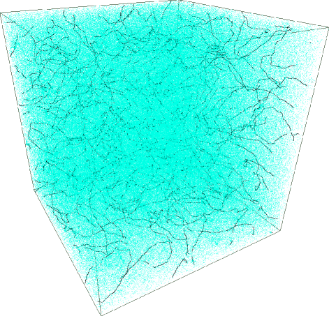
Figure 2: Snapshot of a network of long strings and closed loops in the matter era cmf .

Very recently, numerical simulations of cosmic string evolution in a FLRW Universe (see, Fig. 2), found evidence cmf of a scaling regime for the cosmic string loops in the radiation and matter dominated eras down to the hundredth of the horizon time. It is important to note that the scaling was found without considering any gravitational back reaction effect; it was just the result of string intercmmuting mechanism. As it was reported in Ref. cmf , the scaling regime of string loops appears after a transient relaxation era, driven by a transient overproduction of string loops with length close to the initial correlation length of the string network. Calculating the amount of energy momentum tensor lost from the string network, it was found cmf that a few percents of the total string energy density disappear in the very brief process of formation of numerically unresolved string loops during the very first timesteps of the string evolution. Subsequently, two other studies support these findings vov ,martinsshellard .

2.6 String Thermodynamics

It is one of the basic facts about string theory that the degeneracy of string states increases exponentially with energy,

$$d(E)\sim e^{\beta_{\rm H}E}~{}.$$ (2.63)

A consequence of this is that there is a maximum temperature $T_{\rm max}=1/\beta_{\rm H}$, the Hagedorn temperature hagedorn ; ed1 ; ed2 . In the microcanonical ensemble the description of this situation is as follows: Consider a system of closed string loops in a three-dimensional box. Intersecting strings intercommute, but otherwise they do not interact and are described by the Goto-Nambu equations of motion. The statistical properties of a system of strings in equilibrium are characterised by only one parameter, the energy density of strings, $\rho$,

$$\rho=\frac{E}{L^{3}}~{},$$ (2.64)

where $L$ denotes the size of the cubical box. The behaviour of the system depends on whether it is at low or high energy densities, and it undergoes a phase transition at a critical energy density, the Hagedorn energy density $\rho_{\rm H}$. Quantisation implies a lower cutoff for the size of the string loops, determined by the string tension $\mu$. The lower cutoff on the loop size is roughly $\mu^{-1/2}$, implying that the mass of the smallest string loops is $m_{0}\sim\mu^{1/2}$.

For a system of strings at the low energy density regime ($\rho\ll\rho_{\rm H}$), all strings are chopped down to the loops of the smallest size, while larger loops are exponentially suppressed. Thus, for small enough energy densities, the string equilibrium configuration is dominated by the massless modes in the quantum description. The energy distribution of loops, given by the number $dn$ of loops with energies between $E$ and $E+dE$ per unit volume, is ed1 ; ed2 ; ed3

$$dn\propto e^{-\alpha E}E^{-5/2}dE~{}~{}(\rho\ll\rho_{\rm H})~{},$$ (2.65)

where $\alpha=(5/2m_{0})\ln(\rho_{\rm H}/\rho)$.

However, as we increase the energy density, more and more oscillatory modes of strings get excited. In particular, if we reach a critical energy density, $\rho_{\rm H}$, then long oscillatory string states begin to appear in the equilibrium state. The density at which this happens corresponds to the Hagedorn temperature. The Hagedorn energy density $\rho_{\rm H}$, achieved when the separation between the smallest string loops is of the order of their sizes, is $\rho_{\rm c}\sim m_{0}^{4}$. At the Hagedorn energy density the system undergoes a phase transition characterised by the appearance of infinitely long strings.

At the high energy density regime ($\rho\gg\rho_{\rm c}$), the energy distribution of string loops is ed1 ; ed2 ; ed3

$$dn=Am_{0}^{9/2}E^{-5/2}dE~{}~{}(\rho\gg\rho_{\rm H})~{},$$ (2.66)

where $A$ is a numerical coefficient independent of $m_{0}$ and of $\rho$. Equation (2.66) implies that the mean-square radius $R$ of the closed string loops is

$$R\sim m_{0}^{-3/2}E^{1/2}~{},$$ (2.67)

meaning that large string loops are random walks of step $\sim m_{0}^{-1}$. Equations (2.66) and (2.67) imply

$$dn=A^{\prime}R^{-4}dR~{}~{}(\rho\gg\rho_{\rm H})~{},$$ (2.68)

where $A^{\prime}$ is a numerical constant. From Eq. (2.68) one concludes that the distribution of closed string loops is scale invariant, since it does not depend on the cutoff parameter $m_{0}$.

The total energy density in finite string loops is independent of $\rho$. Increasing the energy density $\rho$ of the system of strings, the extra energy $E-E_{\rm H}$, where $E_{\rm H}=\rho_{\rm H}L^{3}$, goes into the formation of infinitely long strings, implying

$$\rho-\rho_{\rm inf}={\rm const}~{}~{}(\rho\gg\rho_{\rm H})~{},$$ (2.69)

where $\rho_{\rm inf}$ denotes the energy density in infinitely long strings.

Clearly, the above analysis describes the behaviour of a system of strings of low or high energy densities, while there is no analytic description of the phase transition and of the intermediate densities around the critical one, $\rho\sim\rho_{\rm H}$. An experimental approach to the problem has been proposed in Ref. smma1 and later extended in Ref. smed .

The equilibrium properties of a system of cosmic strings have been studied numerically in Ref. smma1 . The strings are moving in a three-dimensional flat space and the initial string states are chosen to be a loop gas consisting of the smallest two-point loops with randomly assigned positions and velocities. This choice is made just because it offers an easily adjustable string energy density. Clearly, the equilibrium state is independent of the initial state. The simulations revealed a distinct change of behaviour at a critical energy density $\rho_{\rm H}=0.0172\pm 0.002$. For $\rho<\rho_{\rm H}$, there are no infinitely long strings, thus their energy density, $\rho_{\rm inf}$, is just zero. For $\rho>\rho_{\rm H}$, the energy density in finite strings is constant, equal to $\rho_{\rm H}$, while the extra energy goes to the infinitely long strings with energy density $\rho_{\rm inf}=\rho-\rho_{\rm H}$. Thus, Eqs. (2.66) and (2.69) are valid for all $\rho>\rho_{\rm H}$, although they were derived only in the limit $\rho\gg\rho_{\rm H}$. At the critical energy density, $\rho=\rho_{\rm H}$, the system of strings is scale-invariant. At bigger energy densities, $\rho>\rho_{\rm H}$, the energy distribution of closed string loops at different values of $\rho$ were found  smma1 to be identical within statistical errors, and well defined by a line $dn/dE\propto E^{-5/2}$. Thus, for $\rho>\rho_{\rm H}$, the distribution of finite strings is still scale-invariant, but in addition the system includes the infinitely long strings, which do not exhibit a scale-invariant distribution. The number distribution for infinitely long strings goes as $dn/dE\propto 1/E$, which means that the total number of infinitely long strings is roughly $\log(E-E_{\rm H})$. So, typically the number of long strings grows very slowly with energy; for $\rho>\rho_{\rm H}$ there are just a few infinitely long strings, which take up most of the energy of the system.

The above numerical experiment has been extended smed for strings moving in a higher dimensional box. The Hagedorn energy density was found for strings moving in boxes of dimensionality $d_{\rm B}=3,4,5$ smed :

$$\rho_{\rm H} = \left\{\begin{array}[]{lcl}0.172\pm 0.002\ \ \mbox{for}&d_{\rm B}=3\\ 0.062\pm 0.001\ \ \mbox{for}&d_{\rm B}=4\\ 0.031\pm 0.001\ \ \mbox{for}&d_{\rm B}=5\end{array}\right.$$ (2.73)

Moreover, the size distribution of closed finite string loops at the high energy density regime was found to be independent of the particular value of $\rho$ for a given dimensionality of the box $d_{\rm B}$. The size distribution of finite closed string loops was foundsmed to be well defined by a line

$$\frac{dn}{dE}\sim E^{-(1+d_{\rm B}/2)}~{},$$ (2.74)

where the space dimensionality $d_{\rm B}$ was taken equal to 3, 4, or 5 . The statistical errors indicated a slope equal to $-(1+d_{\rm B}/2)\pm 0.2$. Above the Hagedorn energy density the system is again characterised by a scale-invariant distribution of finite closed string loops and a number of infinitely long strings with a distribution which is not scale invariant.

2.7 Genericity of Cosmic Strings Formation within SUSY GUTs

The Standard Model (SM), even though it has been tested to a very high precision, is incapable of explaining neutrino masses SK ; SNO ; kamland . An extension of the SM gauge group can be realised within Supersymmetry (SUSY). SUSY offers a solution to the gauge hierarchy problem, while in the supersymmetric extension of the standard model the gauge coupling constants of the strong, weak and electromagnetic interactions meet at a single point, $M_{\rm GUT}\simeq(2-3)\times 10^{16}$ GeV. In addition, SUSY GUTs provide the scalar field which could drive inflation, explain the matter-antimatter asymmetry of the Universe, and propose a candidate, the lightest superparticle, for cold dark matter. We will address the question of whether cosmic string formation is generic, in the context of SUSY GUTs.

Within SUSY GUTs there is a large number of SSB patterns leading from a large gauge group G to the SM gauge group G${}_{\rm SM}\equiv$ SU(3)${}_{\rm C}\times$ SU(2)${}_{\rm L}\times$ U(1)_Y. The study of the homotopy group of the false vacuum for each SSB scheme determines whether there is defect formation and identifies the type of the formed defect. Clearly, if there is formation of domain walls or monopoles, one will have to place an era of supersymmetric hybrid inflation to dilute them. To consider a SSB scheme as a successful one, it should be able to explain the matter/anti-matter asymmetry of the Universe and to account for the proton lifetime measurements SK .

In what follows, we consider a mechanism of baryogenesis via leptogenesis, which can be thermal or nonthermal one. In the case of nonthermal leptogenesis, U(1)_B-L (B and L, are the baryon and lepton numbers, respectively) is a sub-group of the GUT gauge group, G_GUT, and B-L is broken at the end or after inflation. If one considers a mechanism of thermal leptogenesis, B-L is broken independently of inflation. If leptogenesis is thermal and B-L is broken before the inflationary era, then one should check whether the temperature at which B-L is broken — this temperature defines the mass of the right-handed neutrinos — is smaller than the reheating temperature. To have a successful inflationary cosmology, the reheating temperature should be lower than the limit imposed by the gravitino. To ensure the stability of proton, the discrete symmetry Z₂, which is contained in U(1)_B-L, must be kept unbroken down to low energies. Thus, the successful SSB schemes should end at G${}_{\rm SM}\times$ Z₂. Taking all these considerations into account we will examine within all acceptable SSB patterns, how often cosmic strings form at the end of the inflationary era.

To proceed, one has to first choose the large gauge group G_GUT. In Ref. jrs this study has been done in detail for a large number of simple Lie groups. Considering GUTs based on simple gauge groups, the type of supersymmetric hybrid inflation will be of the F-type. The minimum rank of G_GUT has to be at least equal to 4, to contain the G_SM as a subgroup. Then one has to study the possible embeddings of G_SM in G_GUT so that there is an agreement with the SM phenomenology and especially with the hypercharges of the known particles. Moreover, the large gauge group G_GUT must include a complex representation, needed to describe the SM fermions, and it must be anomaly free. In principle, ${\rm SU}(n)$ may not be anomaly free. We thus assume that all ${\rm SU}(n)$ groups we consider have indeed a fermionic representation which certifies that the model is anomaly free. We set as the upper bound on the rank $r$ of the group, $r\leq 8$. Clearly, the choice of the maximum rank is in principle arbitrary. This choice could, in a sense, be motivated by the Horava-Witten hw model, based on ${\rm E}_{8}\times{\rm E}_{8}$. Concluding, the large gauge group G_GUT could be one of the following: SO(10), E₆, SO(14), SU(8), SU(9); flipped SU(5) and [SU(3)]³ are included within this list as subgroups of SO(10) and E₆, respectively.

A detailed study of all SSB schemes which bring us from G_GUT down to the SM gauge group G_SM, by one or more intermediate steps, shows that cosmic strings are generically formed at the end of hybrid inflation. If the large gauge group G_GUT is SO(10) then cosmic strings formation is unavoidable jrs .

The genericity of cosmic string formation for ${\rm E}_{6}$ depends whether one considers thermal or nonthermal leptogenesis. More precisely, under the assumption of nonthermal leptogenesis, cosmic string formation is unavoidable. Considering thermal leptogenesis, cosmic strings formation at the end of hybrid inflation arises in $98\%$ of the acceptable SSB schemes adp . Finally, if the requirement of having Z₂ unbroken down to low energies is relaxed and thermal leptogenesis is considered as the mechanism for baryogenesis, cosmic string formation accompanies hybrid inflation in $80\%$ of the SSB schemes.

The SSB schemes of SU(6) and SU(7) down to the G_SM which could accommodate an inflationary era with no defect (of any kind) at later times are inconsistent with proton lifetime measurements. Minimal SU(6) and SU(7) do not predict neutrino masses jrs , implying that these models are incompatible with high energy physics phenomenology.

Higher rank groups, namely SO(14), SU(8) and SU(9), should in general lead to cosmic string formation at the end of hybrid inflation. In all these schemes, cosmic string formation is sometimes accompanied by the formation of embedded strings. The strings which form at the end of hybrid inflation have a mass which is proportional to the inflationary scale.

3 Cosmic Microwave Background Temperature Anisotropies

The CMB temperature anisotropies offer a powerful test for theoretical models aiming at describing the early Universe. The characteristics of the CMB multipole moments can be used to discriminate among theoretical models and to constrain the parameters space.

The spherical harmonic expansion of the CMB temperature anisotropies, as a function of angular position, is given by

$$\frac{\delta T}{T}({\bf n})=\sum_{\ell m}a_{\ell m}{\cal W}_{\ell}Y_{\ell m}({\bf n})~{}\,\ \ \ \mbox{with}\ \ \ a_{\ell m}=\int{\rm d}\Omega_{{\bf n}}\frac{\delta T}{T}({\bf n})Y_{\ell m}^{*}({\bf n})~{};$$ (3.75)

${\cal W}_{\ell}$ stands for the $\ell$-dependent window function of the particular experiment. The angular power spectrum of CMB temperature anisotropies is expressed in terms of the dimensionless coefficients $C_{\ell}$, which appear in the expansion of the angular correlation function in terms of the Legendre polynomials $P_{\ell}$:

$$\biggl{\langle}0\biggl{|}\frac{\delta T}{T}({\bf n})\frac{\delta T}{T}({\bf n}^{\prime})\biggr{|}0\biggr{\rangle}\left|{}_{{~{}}_{\!\!({\bf n\cdot n}^{\prime}=\cos\vartheta)}}\right.=\frac{1}{4\pi}\sum_{\ell}(2\ell+1)C_{\ell}P_{\ell}(\cos\vartheta){\cal W}_{\ell}^{2}~{},$$ (3.76)

where we have used the addition theorem of spherical harmonics, i.e.,

$$\sum_{m=-\ell}^{\ell}Y_{\ell m}({\bf n})Y_{\ell m}^{\star}({\bf n}^{\prime})=\frac{2\ell+1}{4\pi}P_{\ell}({\bf n}\cdot{\bf n}^{\prime})~{}.$$ (3.77)

It compares points in the sky separated by an angle $\vartheta$. Here, the brackets denote spatial average, or expectation values if perturbations are quantised. Equation (3.76) holds only if the initial state for cosmological perturbations of quantum-mechanical origin is the vacuum jam ; gms . The value of $C_{\ell}$ is determined by fluctuations on angular scales of the order of $\pi/\ell$. The angular power spectrum of anisotropies observed today is usually given by the power per logarithmic interval in $\ell$, plotting $\ell(\ell+1)C_{\ell}$ versus $\ell$.

To find the power spectrum induced by topological defects, one has to solve, in Fourier space for each given wave vector ${\bf k}$ a system of linear perturbation equations with random sources:

$${\cal D}X={\cal S}~{},$$ (3.78)

where ${\cal D}$ denotes a time dependent linear differential operator, $X$ is a vector which contains the various matter perturbation variables, and ${\cal S}$ is the random source term, consisting of linear combinations of the energy momentum tensor of the defect. For given initial conditions, Eq. (3.78) can be solved by means of a Green’s function, ${\cal G}(\tau,\tau^{\prime})$, in the form

$$X_{j}(\tau_{0},{\bf k})=\int_{\tau_{in}}^{\tau_{0}}\!d\tau{\cal G}_{jm}(\tau_{0},\tau,{\bf k}){\cal S}_{m}(\tau,{\bf k})~{}.$$ (3.79)

To compute power spectra or, more generally, quadratic expectation values of the form $\langle X_{j}(\tau_{0},{\bf k})X_{m}^{*}(\tau_{0},{\bf k^{\prime}})\rangle$, one has to calculate

$$\langle X_{j}(\tau_{0},{\bf k})X_{l}^{\star}(\tau_{0},{\bf k}^{\prime})\rangle=$$ (3.80)

$$\ \ \ \ \ \ \ \ \int_{\tau_{in}}^{\tau_{0}}\!d\tau{\cal G}_{jm}(\tau,{\bf k})\int_{\tau_{in}}^{\tau_{0}}\!d\tau^{\prime}{\cal G}^{\star}_{ln}(\tau^{\prime},{\bf k}^{\prime})\times\langle{\cal S}_{m}(\tau,{\bf k}){\cal S}_{n}^{\star}(\tau^{\prime},{\bf k}^{\prime})\rangle~{}.$$ (3.81)

Thus, to compute power spectra, one should know the unequal time two-point correlators $\langle{\cal S}_{m}(\tau,{\bf k}){\cal S}_{n}^{\star}(\tau^{\prime},{\bf k}^{\prime})\rangle$ in Fourier space Hindarsh . This object is calculated by means of heavy numerical simulations.

The CMB temperature anisotropies provide a powerful tool to discriminate among inflation and topological defects. On large angular scales ($\ell\lesssim 50$), both families of models lead to approximately scale-invariant spectra, with however a different prediction regarding the statistics of the induced perturbations. Provided the quantum fields are initially placed in the vacuum, inflation predicts generically Gaussian fluctuations, whereas in the case of topological defect models, the induced perturbations are clearly nongaussian, at least at sufficiently high angular resolution. This is an interesting fingerprint, even though difficult to test through the data. In the context of inflation, nongaussianity can however also be present, as for example in the case of stochastic inflation stochastic , or in a class of inflationary models involving two scalar fields leading to nongaussian isothermal fluctuations with a blue spectrum linde1 . In addition, allowing nonvacuum initial states for the cosmological perturbations of quantum-mechanical origin, one generically obtains a non-Gaussian spectrum jam ; gms , in the context of single-field inflation.

On intermediate and small angular scales however, the predictions of inflation are quite different than those of topological defect models, due to the different nature of the induced perturbations. On the one hand, the inflationary fluctuations are coherent, in the sense that the perturbations are initially at the same phase and subsequently evolve linearly and independently of each other. The subsequent progressive phase shift between different modes produces the acoustic peak structure. On the other hand, in topological defect models, fluctuations are constantly induced by the sources (defects). Since topological defects evolve in a nonlinear manner, and since the random initial conditions of the source term in the perturbation equations of a given scale leaks into other scales, perfect coherence is destroyed. The predictions of the defects models regarding the characteristics of the CMB spectrum are:

• Global ${\cal O}(4)$ textures lead to a position of the first acoustic peak at $\ell\simeq 350$ with an amplitude $\sim 1.5$ times higher than the Sachs-Wolfe plateau rm .

• Global ${\cal O}(N)$ textures in the large $N$ limit lead to a quite flat spectrum, with a slow decay after $\ell\sim 100$ dkm . Similar are the predictions of other global ${\cal O}(N)$ defects clstrings ; num .

• Local cosmic strings simulations csmark found a broad peak at $\ell\approx 150-400$, being produced from both vector and scalar modes, which peaks at $\ell\approx 180$ and $\ell\approx 400$ respcetively.

The position and amplitude of the acoustic peaks, as found by the CMB measurements maxi ; boom ; dasi ; wmap , are in disagreement with the predictions of topological defect models. As a consequence, CMB measurements rule out pure topological defect models as the origin of initial density perturbations leading to the observed structure formation.

3.1 Mixed Models

Since cosmic strings are expected to be generically formed in the context of SUSY GUTs, one should consider mixed perturbation models where the dominant rôle is played by the inflaton field but cosmic strings have also a contribution, small but not negligible. Restricting ourselves to the angular power spectrum, we can remain in the linear regime. In this case,

$$C_{\ell}=\alpha C^{\scriptscriptstyle{\rm I}}_{\ell}+(1-\alpha)C^{\scriptscriptstyle{\rm S}}_{\ell}~{},$$ (3.82)

where $C^{\scriptscriptstyle{\rm I}}_{\ell}$ and $C^{\scriptscriptstyle{\rm S}}_{\ell}$ denote the (COBE normalized) Legendre coefficients due to adiabatic inflaton fluctuations and those stemming from the cosmic string network, respectively. The coefficient $\alpha$ in Eq. (3.82) is a free parameter giving the relative amplitude for the two contributions. Comparing the $C_{\ell}$, calculated using Eq. (3.82) — where $C^{\scriptscriptstyle{\rm I}}_{\ell}$ is taken from a generic inflationary model and $C^{\scriptscriptstyle{\rm S}}_{\ell}$ from numerical simulations of cosmic string networks — with data obtained from the most recent CMB measurements, one gets that a cosmic string contribution to the primordial fluctuations higher than $14\%$ is excluded up to $95\%$ confidence level bprs ; pogosian ; wyman (see, Fig. 3).

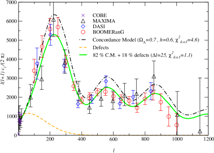
Figure 3: $\ell(\ell+1)C_{\ell}$ versus $\ell$ for three different models. The string contribution turns out to be $\sim 18\%$ of the total bprs .

In what follows, we follow a conservative approach and do not allow cosmic strings to contribute more than $10\%$ to the CMB temperature anisotropies.

3.2 Supersymmetric Hybrid Inflation

Inflation offers simple answers to the shortcomings of the standard hot big bang model. In addition, simple inflationary models offer successful candidates for the initial density fluctuations leading to the observed structure formation.

One crucial question though is to answer how generic is the onset of inflation ecms ; gt ; us and to find consistent and natural models of inflation from the point of view of particle physics. Even though one can argue that the initial conditions which favor inflationary models are the likely outcome of the quantum era before inflation ecms , one should then show that inflation will last long enough to solve the shortcomings of the standard hot big bang model gt ; us . In addition, to find natural ways to guarantee the flatness of the inflaton potential remains a difficult task. Inflation is, unfortunately, still a paradigm in search of a model. It is thus crucial to identify successful but natural inflationary models motivated from high energy physics.

In what follows we discuss two well-studied inflationary models in the framework of supersymmetry, namely F/D-term inflation. Our aim is to check the compatibility of these models — here cosmic string inflation is generic — with the CMB and gravitino constraints.

F-term Inflation

F-term inflation can be naturally accommodated in the framework of GUTs, when a GUT gauge group G_GUT is broken down to the G_SM at an energy $M_{\rm GUT}$, according to the scheme

$${\rm G}_{\rm GUT}\stackrel{{\scriptstyle M_{\rm GUT}}}{{\hbox to22.76228pt{\rightarrowfill}}}{\rm H}_{1}\,\lower 9.0pt\hbox{$\stackrel{{\scriptstyle\stackrel{{\scriptstyle\displaystyle M_{\rm infl}}}{{\hbox to28.45274pt{\rightarrowfill}}}}}{{\Phi_{+}\Phi_{-}}}$}\,{\rm H}_{2}{\longrightarrow}{\rm G}_{\rm SM}~{};$$ (3.83)

$\Phi_{+},\Phi_{-}$ is a pair of GUT Higgs superfields in nontrivial complex conjugate representations, which lower the rank of the group by one unit when acquiring nonzero vacuum expectation value. The inflationary phase takes place at the beginning of the symmetry breaking ${\rm H}_{1}\stackrel{{\scriptstyle M_{\rm infl}}}{{\longrightarrow}}{\rm H}_{2}$.

F-term inflation is based on the globally supersymmetric renormalisable superpotential

$$W_{\rm infl}^{\rm F}=\kappa S(\Phi_{+}\Phi_{-}-M^{2})~{},$$ (3.84)

where $S$ is a GUT gauge singlet left handed superfield, $\Phi_{+}$ and $\Phi_{-}$ are defined above; $\kappa$ and $M$ are two constants ($M$ has dimensions of mass) which can be taken positive with field redefinition. The chiral superfields $S,\Phi_{+},\Phi_{-}$ are taken to have canonical kinetic terms. This superpotential is the most general one consistent with an R-symmetry under which $W\rightarrow e^{i\beta}W~{},\Phi_{-}\rightarrow e^{-i\beta}\Phi_{-}~{},\Phi_{+}\rightarrow e^{i\beta}\Phi_{+}$, and $S\rightarrow e^{i\beta}S$. An R-symmetry can ensure that the rest of the renormalisable terms are either absent or irrelevant.

The scalar potential reads

$$V(\phi_{+},\phi_{-},S)=|F_{\Phi_{+}}|^{2}+|F_{\Phi_{-}}|^{2}+|F_{S}|^{2}+\frac{1}{2}\sum_{a}g_{a}^{2}D_{a}^{2}~{}.$$ (3.85)

The F-term is such that $F_{\Phi_{i}}\equiv|\partial W/\partial\Phi_{i}|_{\theta=0}$, where we take the scalar component of the superfields once we differentiate with respect to $\Phi_{i}=\Phi_{+},\Phi_{-},S$. The D-terms are

$$D_{a}=\bar{\phi}_{i}\,{(T_{a})^{i}}_{j}\,\phi^{j}+\xi_{a}~{},$$ (3.86)

with $a$ the label of the gauge group generators $T_{a}$, $g_{a}$ the gauge coupling, and $\xi_{a}$ the Fayet-Iliopoulos term. By definition, in the F-term inflation the real constant $\xi_{a}$ is zero; it can only be nonzero if $T_{a}$ generates an extra U(1) group. In the context of F-term hybrid inflation, the F-terms give rise to the inflationary potential energy density, while the D-terms are flat along the inflationary trajectory, thus one may neglect them during inflation.

The potential has one valley of local minima, $V=\kappa^{2}M^{4}$, for $S>M$ with $\phi_{+}=\phi_{-}=0$, and one global supersymmetric minimum, $V=0$, at $S=0$ and $\phi_{+}=\phi_{-}=M$. Imposing initially $S\gg M$, the fields quickly settle down the valley of local minima. Since in the slow roll inflationary valley, the ground state of the scalar potential is nonzero, SUSY is broken. In the tree level, along the inflationary valley the potential is constant, therefore perfectly flat. A slope along the potential can be generated by including the one-loop radiative corrections. Thus, the scalar potential gets a little tilt which helps the inflaton field $S$ to slowly roll down the valley of minima. The one-loop radiative corrections to the scalar potential along the inflationary valley, lead to an effective potential DvaShaScha ; Lazarides ; SenoSha ; rs1

$$V_{\rm eff}^{\rm F}(|S|) =\kappa^{2}M^{4}\biggl{\{}1+\frac{\kappa^{2}\cal{N}}{32\pi^{2}}\biggl{[}2\ln\frac{|S|^{2}\kappa^{2}}{\Lambda^{2}}$$ (3.88)

$$+\biggl{(}\frac{|S|^{2}}{M^{2}}+1\biggr{)}^{2}\ln\big{(}1+\frac{M^{2}}{|S|^{2}})+\biggl{(}\frac{|S|^{2}}{M^{2}}-1\biggr{)}^{2}\ln\biggl{(}1-\frac{M^{2}}{|S|^{2}}\biggr{)}\biggr{]}\biggr{\}}$$

where $\Lambda$ is a renormalisation scale and $\cal{N}$ stands for the dimensionality of the representation to which the complex scalar components $\phi_{+},\phi_{-}$ of the chiral superfields $\Phi_{+},\Phi_{-}$ belong. For example, ${\cal N}={\bf 27,126,351}$, correspond to realistic SSB schemes in SO(10), or E₆ models.

Considering only large angular scales, i.e., taking only the Sachs-Wolfe contribution, one can get the contributions to the CMB temperature anisotropies analytically. The quadrupole anisotropy has one contribution coming from the inflaton field, splitted into scalar and tensor modes, and one contribution coming from the cosmic string network, given by numerical simulations ls . The inflaton field contribution is

$$\biggl{(}\frac{\delta T}{T}\biggr{)}_{\rm Q-infl}=\biggl{[}\biggl{(}\frac{\delta T}{T}\biggr{)}^{2}_{\rm Q-scal}+\biggl{(}\frac{\delta T}{T}\biggr{)}^{2}_{\rm Q-tens}\biggr{]}^{1/2}~{},$$ (3.89)

where the quadrupole anisotropy due to the scalar and tensor Sachs-Wolfe effect is

$$\biggl{(}\frac{\delta T}{T}\biggr{)}_{\rm Q-scal} = \frac{1}{4\sqrt{45}\pi}\frac{V^{3/2}(\varphi_{\rm Q})}{M^{3}_{\rm Pl}V^{\prime}(\varphi_{\rm Q})}$$ (3.90)

$$\biggl{(}\frac{\delta T}{T}\biggr{)}_{\rm Q-tens} \sim \frac{0.77}{8\pi}\frac{V^{1/2}(\varphi_{\rm Q})}{M^{2}_{\rm Pl}}~{},$$ (3.91)

respectively, with $V^{\prime}\equiv dV(\varphi)/d\varphi$, $M_{\rm Pl}$ the reduced Planck mass, $M_{\rm Pl}=(8\pi G)^{-1/2}\simeq 2.43\times 10^{18}{\rm GeV}$, and $\varphi_{\rm Q}$ the value of the inflaton field when the comoving scale corresponds to the quadrupole anisotropy became bigger than the Hubble radius. It can be calculated using Eqs. (3.88),(3.89),(3.91).

Fixing the number of e-foldings to 60, the inflaton and cosmic string contribution to the CMB, for a given gauge group G_GUT, depend on the superpotential coupling $\kappa$, or equivalently on the symmetry breaking scale $M$ associated with the inflaton mass scale, which coincides with the string mass scale. The relation between $\kappa$ and $M$ is

$$\frac{M}{M_{\rm Pl}}=\frac{\sqrt{N_{\rm Q}\cal N}\,\kappa}{2\,\pi\,y_{\rm Q}}~{},$$ (3.92)

where

$$y_{\rm Q}^{2}=\int_{1}^{\frac{|S_{\rm Q}|^{2}}{M^{2}}}dz\biggl{[}z\big{\{}(z+1)\ln(1+z^{-1})+(z-1)\ln(1-z^{-1})\bigl{\}}\big{]}~{}.$$ (3.93)

The total quadrupole anisotropy has to be normalised to the COBE data.

A detailed study has been performed in Ref. rs1 . It was shown that the cosmic string contribution is consistent with the CMB measurements, provided rs1

$$M\hbox{ \raise 1.50696pt\hbox to0.0pt{$<$\hss}\lower 2.58334pt\hbox{$\sim$}\ }2\times 10^{15}{\rm GeV}~{}~{}\Leftrightarrow~{}~{}\kappa\hbox{ \raise 1.50696pt\hbox to0.0pt{$<$\hss}\lower 2.58334pt\hbox{$\sim$}\ }7\times 10^{-7}~{}.$$ (3.94)

In Fig.4, one can see the contribution of cosmic strings to the quadrupole anisotropy as a function of the superpotential coupling $\kappa$ rs1 . The three curves correspond to $\mathcal{N}=\mathbf{27}$ (curve with broken line), $\mathcal{N}=\mathbf{126}$ (full line) and $\mathcal{N}=\mathbf{351}$ (curve with lines and dots).

Figure 4: Contribution of cosmic strings to the quadrupole anisotropy as a function of the superpotential coupling $\kappa$. The three curves correspond to $\mathcal{N}=\mathbf{27}$ (curve with broken line), $\mathcal{N}=\mathbf{126}$ (full line) and $\mathcal{N}=\mathbf{351}$ (curve with lines and dots) rs1 .

The constraint on $\kappa$ given in Eq. (3.94) is in agreement with the one found in Ref. lk . Strictly speaking the above condition was found in the context of SO(10) gauge group, but the conditions imposed in the context of other gauge groups are of the same order of magnitude since $M$ is a slowly varying function of the dimensionality ${\cal N}$ of the representations to which the scalar components of the chiral Higgs superfields belong.

The superpotential coupling $\kappa$ is also subject to the gravitino constraint which imposes an upper limit to the reheating temperature, to avoid gravitino overproduction. The reheating temperature $T_{\rm RH}$ characterises the reheating process via which the Universe enters the high entropy radiation dominated phase at the end of the inflationary era. Within the minimal supersymmetric standard model and assuming a see-saw mechanism to give rise to massive neutrinos, the reheating temperature is rs1

$$T_{\rm RH}\approx\frac{(8\pi)^{1/4}}{7}(\Gamma M_{\rm Pl})^{1/2}~{},$$ (3.95)

where $\Gamma$ is the decay width of the oscillating inflaton and Higgs fields into right-handed neutrinos

$$\Gamma=\frac{1}{8\pi}\biggl{(}\frac{M_{i}}{M}\biggr{)}^{2}m_{\rm infl}~{};$$ (3.96)

with $m_{\rm infl}=\sqrt{2}\kappa M$ the inflaton mass and $M_{i}$ the right-handed neutrino mass eigenvalue with $M_{i}<m_{\rm infl}/2$. Equations (3.92), (3.95), (3.96) lead to

$$T_{\rm RH}\sim\frac{1}{12}\left(\frac{60}{N_{\rm Q}}\right)^{1/4}\left(\frac{1}{{\cal N}}\right)^{1/4}y_{\rm Q}^{1/2}M_{i}~{}.$$ (3.97)

In order to have successful reheating, it is important not to create too many gravitinos, which imply the following constraint on the reheating temperature gr $T_{\rm RH}\leq 10^{9}{\rm GeV}$. Since the two heaviest neutrinos are expected to have masses of the order of $M_{3}\simeq 10^{15}$ GeV and $M_{2}\simeq 2.5\times 10^{12}$ GeV respectively pati , $M_{i}$ is identified with $M_{1}\sim 6\times 10^{9}$ GeV pati . The gravitino constraint on $\kappa$ reads rs1 $\kappa\hbox{ \raise 1.50696pt\hbox to0.0pt{$<$\hss}\lower 2.58334pt\hbox{$\sim$}\ }8\times 10^{-3}$, which is clearly a weaker constraint than the one imposed from the CMB data.

Concluding, F-term inflation leads generically to cosmic string formation at the end of the inflationary era. The cosmic strings formed are of the GUT scale. This class of models can be compatible with CMB measurements, provided the superpotential coupling is smaller than $10^{-6}$ . This tuning of the free parameter $\kappa$ can be softened if one allows for the curvaton mechanism.

According to the curvaton mechanism lw2002 ; mt2001 , another scalar field, called the curvaton, could generate the initial density perturbations whereas the inflaton field is only responsible for the dynamics of the Universe. The curvaton is a scalar field, that is sub-dominant during the inflationary era as well as at the beginning of the radiation dominated era which follows the inflationary phase. There is no correlation between the primordial fluctuations of the inflaton and curvaton fields. Clearly, within supersymmetric theories such scalar fields are expected to exist. In addition, embedded strings, if they accompany the formation of cosmic strings, they may offer a natural curvaton candidate, provided the decay product of embedded strings gives rise to a scalar field before the onset of inflation. Considering the curvaton scenario, the coupling $\kappa$ is only constrained by the gravitino limit. More precisely, assuming the existence of a curvaton field, there is an additional contribution to the temperature anisotropies. The WMAP CMB measurements impose rs1 the following limit on the initial value of the curvaton field

$${\cal\psi}_{\rm init}\hbox{ \raise 1.50696pt\hbox to0.0pt{$<$\hss}\lower 2.58334pt\hbox{$\sim$}\ }5\times 10^{13}\,\left(\frac{\kappa}{10^{-2}}\right){\rm GeV}~{},$$ (3.98)

provided the parameter $\kappa$ is in the range $[10^{-6},~{}1]$ (see, Fig. 5).

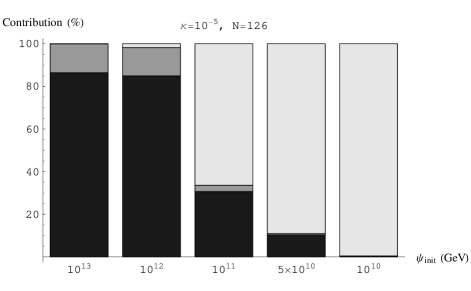
Figure 5: The cosmic strings (dark gray), curvaton (light gray) and inflaton (gray) contributions to the CMB temperature anisotropies as a function of the the initial value of the curvaton field ${\cal\psi}_{\rm init}$, and the superpotential coupling $\kappa$, for ${\cal N}=\mathbf{126}$ rs1 .

The above results hold also if one includes supergravity corrections. This is expected since the value of the inflaton field is several orders of magnitude below the Planck scale.

D-term Inflation

The early history of the Universe at energies below the Planck scale is described by an effective N=1 supergravity (SUGRA) theory. Inflation should have taken place at an energy scale $V^{1/4}\lesssim 4\times 10^{16}$ GeV, implying that inflationary models should be constructed in the framework of SUGRA.

However, it is difficult to implement slow-roll inflation within SUGRA. The positive false vacuum of the inflaton field breaks spontaneously global supersymmetry, which gets restored after the end of inflation. In supergravity theories, the supersymmetry breaking is transmitted to all fields by gravity, and thus any scalar field, including the inflaton, gets an effective mass of the order of the the expansion rate $H$ during inflation.

This problem, known as the problem of Hubble-induced mass, originates from F-term interactions — note that it is absent in the model we have described in the previous subsection — and thus it is resolved if one considers the vacuum energy as being dominated by non-zero D-terms of some superfields dterm1 ; dterm2 . This result led to a dramatic interest in D-term inflation, since in addition, it can be easily implemented within string theory.

D-term inflation is derived from the superpotential

$$W^{\rm D}_{\rm infl}=\lambda S\Phi_{+}\Phi_{-}~{};$$ (3.99)

$S,\Phi_{-},\Phi_{+}$ are three chiral superfields and $\lambda$ is the superpotential coupling. D-term inflation requires the existence of a nonzero Fayet-Iliopoulos term $\xi$, which can be added to the Lagrangian only in the presence of an extra U(1) gauge symmetry, under which, the three chiral superfields have charges $Q_{S}=0$, $Q_{\Phi_{+}}=+1$, and $Q_{\Phi_{-}}=-1$. This extra U(1) gauge symmetry can be of a different origin; hereafter we consider a nonanomalous U(1) gauge symmetry. Thus, D-term inflation requires a scheme, like

$${\rm G}_{\rm GUT}\times{\rm U}(1)\stackrel{{\scriptstyle M_{\rm GUT}}}{{\hbox to22.76228pt{\rightarrowfill}}}{\rm H}\times{\rm U}(1)\,\lower 9.0pt\hbox{$\stackrel{{\scriptstyle\stackrel{{\scriptstyle\displaystyle M_{\rm nfl}}}{{\hbox to28.45274pt{\rightarrowfill}}}}}{{\Phi_{+}\Phi_{-}}}$}\,{\rm H}\rightarrow{\rm G}_{\rm SM}~{}.$$ (3.100)

The symmetry breaking at the end of the inflationary phase implies that cosmic strings are always formed at the end of D-term hybrid inflation. To avoid cosmic strings, several mechanisms have been proposed which either consider more complicated models or require additional ingredients. For example, one can add a nonrenormalisable term in the potential shifted , or add an additional discrete symmetry smooth , or consider GUT models based on nonsimple groups mcg , or introduce a new pair of charged superfields jaa so that cosmic string formation is avoided at the end of D-term inflation. In what follows, we show that standard D-term inflation followed unavoidably by cosmic string production is compatible with CMB data, because the cosmic string contribution to the CMB data is not constant nor dominant. Thus, one does not have to invoke some new physics.

In the global supersymmetric limit, Eqs. (3.85), (3.99) lead to the following expression for the scalar potential

$$V^{\rm D}(\phi_{+},\phi_{-},S)=\lambda^{2}\left[\,|S|^{2}(|\phi_{+}|^{2}+|\phi_{-}|^{2})+|\phi_{+}\phi_{-}|^{2}\right]+\frac{g^{2}}{2}(|\phi_{+}|^{2}-|\phi_{-}|^{2}+\xi)^{2}~{},$$ (3.101)

where $g$ is the gauge coupling of the U(1) symmetry and $\xi$ is a Fayet-Iliopoulos term, chosen to be positive.

In D-term inflation, as opposed to F-term inflation, the inflaton mass acquires values of the order of Planck mass, and therefore, the correct analysis must be done in the framework of SUGRA. The SSB of SUSY in the inflationary valley introduces a splitting in the masses of the components of the chiral superfields $\Phi_{\pm}$. As a result, we obtain rs2 two scalars with squared masses $m^{2}_{\pm}=\lambda^{2}|S|^{2}\exp\left(|S|^{2}/M^{2}_{\rm Pl}\right)\pm g^{2}\xi$ and a Dirac fermion with squared mass $m_{\rm f}^{2}=\lambda^{2}|S|^{2}\exp\left(|S|^{2}/M^{2}_{\rm Pl}\right)$. Calculating the radiative corrections, the effective scalar potential for minimal supergravity reads rs1 ; rs2

$$V_{\rm eff}=\frac{g^{2}\xi^{2}}{2}\biggl{\{}1+\frac{g^{2}}{16\pi^{2}} \times\biggl{[}2\ln\frac{|S|^{2}\lambda^{2}}{\Lambda^{2}}e^{\frac{|S|^{2}}{M^{2}_{\rm Pl}}}$$ (3.102)

$$+ \biggl{(}\frac{\lambda^{2}|S|^{2}}{g^{2}\xi}e^{\frac{|S|^{2}}{M_{\rm Pl}^{2}}}+1\biggr{)}^{2}\ln\biggl{(}1+\frac{g^{2}\xi}{\lambda^{2}|S|^{2}}e^{-\frac{|S|^{2}}{M_{\rm Pl}^{2}}}\biggr{)}$$ (3.103)

$$+ \biggl{(}\frac{\lambda^{2}|S|^{2}}{g^{2}\xi}e^{\frac{|S|^{2}}{M_{\rm Pl}^{2}}}-1\biggr{)}^{2}\ln\biggl{(}1-\frac{g^{2}\xi}{\lambda^{2}|S|^{2}}e^{-\frac{|S|^{2}}{M_{\rm Pl}^{2}}}\biggr{)}\biggr{]}\biggr{\}}$$ (3.104)

As it was explicitely shown in Refs. rs1 ; rs2 , D-term inflation can be compatible with current CMB measurements; the cosmic strings contribution to the CMB is model-dependent. The results obtained in Refs. rs1 ; rs2 can be summarised as follows: (i) $g\hbox{ \raise 1.50696pt\hbox to0.0pt{$>$\hss}\lower 2.58334pt\hbox{$\sim$}\ }2\times 10^{-2}$ is incompatible with the allowed cosmic string contribution to the WMAP measurements; (ii) for $g\hbox{ \raise 1.50696pt\hbox to0.0pt{$<$\hss}\lower 2.58334pt\hbox{$\sim$}\ }2\times 10^{-2}$ the constraint on the superpotential coupling $\lambda$ reads $\lambda\hbox{ \raise 1.50696pt\hbox to0.0pt{$<$\hss}\lower 2.58334pt\hbox{$\sim$}\ }3\times 10^{-5}$; (iii) SUGRA corrections impose in addition a lower limit to $\lambda$; (iv) the constraints induced on the couplings by the CMB measurements can be expressed as a single constraint on the Fayet-Iliopoulos term $\xi$, namely $\sqrt{\xi}\hbox{ \raise 1.50696pt\hbox to0.0pt{$<$\hss}\lower 2.58334pt\hbox{$\sim$}\ }2\times 10^{15}~{}{\rm GeV}$. They are shown in Fig. [6].

Figure 6: Cosmic string contribution to the CMB temperature anisotropies as a function of the superpotential coupling $\lambda$ for different values of the gauge coupling $g$. The maximal contribution allowed by WMAP is represented by a dotted line rs1 ; rs2 .

Assuming the existence of a curvaton field, the fine tuning on the couplings can be avoided provided rs1 ; rs2

$$\psi_{\rm init}\hbox{ \raise 1.50696pt\hbox to0.0pt{$<$\hss}\lower 2.58334pt\hbox{$\sim$}\ }3\times 10^{14}\left(\frac{g}{10^{-2}}\right)~{}{\rm GeV}~{}~{}~{}{\rm for}~{}~{}\lambda\in[10^{-1},10^{-4}]~{}.$$ (3.105)

Clearly, for smaller values of $\lambda$, the curvaton mechanism is not necessary. We show in Fig. 7 the three contributions as a function of $\psi_{\rm init}$, for $\lambda=10^{-1}$ and $g=10^{-1}$. There are values of $\psi_{\rm init}$ which allow bigger values of the superpotential coupling $\lambda$ and of the gauge coupling $g$, than the upper bounds obtained in the absence of a curvaton field.

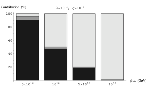
Figure 7: The cosmic strings (dark gray), curvaton (light gray) and inflaton (gray) contributions to the CMB temperature anisotropies as a function of the the initial value of the curvaton field ${\cal\psi}_{\rm init}$, for $\lambda=10^{-1}$ and $g=10^{-1}$ rs2 .

Concluding, standard D-term inflation always leads to cosmic string formation at the end of the inflationary era; these cosmic strings are of the grand unification scale. This class of models is still compatible with CMB measurements, provided the couplings are small enough. As in the case of F-term inflation the fine tuning of the couplings can be softened provided one considers the curvaton mechanism. In this case, the imposed CMB constraint on the initial value of the curvaton field reads rs1 ; rs2

$$\psi_{\rm init}\hbox{ \raise 1.50696pt\hbox to0.0pt{$<$\hss}\lower 2.58334pt\hbox{$\sim$}\ }3\times 10^{14}\left(\frac{g}{10^{-2}}\right)~{}{\rm GeV}~{},~{}~{}\mbox{for}~{}~{}\lambda\in[10^{-1},10^{-4}]~{}.$$ (3.106)

The above conclusions are still valid in the revised version of D-term inflation, in the framework of SUGRA with constant Fayet-Iliopoulos terms. In the context of N=1, 3+1 SUGRA, the presence of constant Fayet-Iliopoulos terms shows up in covariant derivatives of all fermions. In addition, since the relevant local U(1) symmetry is a gauged R-symmetry toine2 , the constant Fayet-Iliopoulos terms also show up in the supersymmetry transformation laws. In Ref. toine1 there were presented all corrections of order $g\xi/M_{\rm Pl}^{2}$ to the classical SUGRA action required by local supersymmetry. Under U(1) gauge transformations in the directions in which there are constant Fayet-Iliopoulos terms $\xi$, the superpotential must transform as toine2

$$\delta W=-i\frac{g\xi}{M_{\rm Pl}^{2}}W~{},$$ (3.107)

otherwise the constant Fayet-Iliopoulos term $\xi$ vanishes. This requirement is consistent with the fact that in the gauge theory at $M_{\rm Pl}\rightarrow\infty$ the potential is U(1) invariant. To promote the simple SUSY D-term inflation model, Eq. (3.99), to SUGRA with constant Fayet-Iliopoulos terms, one has to change the charge assignments for the chiral superfields, so that the superpotential transforms under local R-symmetry toine1 . In SUSY, the D-term potential is neutral under U(1) symmetry, while in SUGRA the total charge of $\Phi_{\pm}$ fields does not vanish but is equal to $-\xi/M_{\rm Pl}^{2}$. More precisely, the D-term contribution to the scalar potential $V$ [see Eq. (3.101)], should be replaced by $(g^{2}/2)(q_{+}|\phi_{+}|^{2}+q_{-}|\phi_{-}|^{2}+\xi)^{2}$ where

$$q_{\pm}=\pm 1-\rho_{\pm}\frac{\xi}{M_{\rm Pl}^{2}}\ \ \ \ \mbox{with}\ \ \ \ \rho_{+}+\rho_{-}=1~{}.$$ (3.108)

In addition, the squared masses of the scalar components $\phi_{\pm}$ become

$$m^{2}_{\pm}=\lambda^{2}|S|^{2}\exp\left(|S|^{2}/M^{2}_{\rm Pl}\right)\pm g^{2}\xi q_{\pm}~{};$$ (3.109)

the Dirac fermion mass remains unchanged.

For the limits we imposed on the Fayet-Iliopoulos term $\xi$, the correction $\xi/M_{\rm Pl}^{2}$ is $\sim 10^{-6}$, implying that the constraints we obtained on $g$ and $\lambda$, or equivalently on $\sqrt{\xi}$, as well as the constraint on $\psi_{\rm init}$ still hold in the revised version of D-term inflation within SUGRA adp .

It is important to generalise the above study in the case of nonminimal SUGRA inprep , in order to know whether qualitatively the above picture remains valid. A recent study inprep has shown that non-minimal Kähler potential do not avoid the fine tuning, since the cosmic string contribution remains dominant unless the couplings and mass scales are small. For example, taking into account higher order corrections in the Kähler potential, or considering supergravity with shift symmetry, we have obtained inprep that the $9\%$ constraint in the allowed contribution of cosmic strings in the CMB spectrum implies

$$\sqrt{\xi}\leq 2\times 10^{15}{\rm GeV}\ \Leftrightarrow\ G\mu\leq 8\times 10^{-7}~{}.$$ (3.110)

The cosmic string problem can be definitely cured if one considers more complicated models, for example where strings become topologically unstable, namely semi-local strings.

4 Cosmic Superstrings

At first, and for many years, cosmic strings and superstrings were considered as two well separated issues. The main reason for this clear distinction may be considered the Planckian tension of superstrings. If the string mass scale is of the order of the Planck mass, then the four-dimensional F- and D-string self gravity is $G_{4}\mu_{\rm F}\sim{\cal O}(g_{\rm s}^{2})$ and $G_{4}\mu_{{\rm D}1}\sim{\cal O}(g_{\rm s})$ ($g_{\rm s}$ stands for the string coupling), respectively, while current CMB measurements impose an upper limit on the self gravity of strings of $G\mu<10^{-6}$. Moreover, heavy superstrings could have only been produced before inflation, and therefore diluted. In addition, Witten showed witten that, in the context of the heterotic theory, long fundamental BPS strings are unstable, thus they would not survive on cosmic time scales; non-BPS strings were also believed to be unstable.

At present, the picture has been dramatically changed (for a review, see e.g., Ref. maj ). In the framework of braneworld cosmology, our Universe represents a three-dimensional Dirichlet brane (D3-brane) on which open fundamental strings (F-strings) end Polch . Such a D3-brane is embedded in a higher dimensional space, the bulk. Brane interactions can unwind and evaporate higher dimensional branes, leaving behind D3-branes embedded in a higher dimensional bulk; one of these D3-branes could play the rôle of our Universe dks . Large extra dimensions can be employed to address the hierarchy problem Ark , a result which lead to an increasing interest in braneworld scenarios. As it has been argued jst ; st D-brane-antibrane inflation leads to the production of lower-dimensional D-branes, that are one-dimensional (D-strings) in the noncompact directions. The production of zero- and two-dimensional defects (monopoles and domain walls, respectively) is suppressed. The large compact dimensions and the large warp factors can allow for superstrings of much lower tensions, in the range between $10^{-11}<G\mu<10^{-6}$. Depending on the model of string theory inflation, one can identify cmp D-strings, F-strings, bound states of $p$ fundamental strings and $q$ D-strings for relatively prime $(p,q)$, or no strings at all.

The probability that two colliding superstrings reconnect can be much less than one. Thus, a reconnection probability ${\cal P}<1$ is one of the distinguishing features of superstrings. D-strings can miss each other in the compact dimension, leading to a smaller ${\cal P}$, while for F-strings the scattering has to be calculated quantum mechanically, since these are quantum mechanical objects.

The collisions between all possible pairs of superstrings have been studied in string perturbation theory jjp . For F-strings, the reconnection probability is of the order of $g_{\rm s}^{2}$. For F-F string collisions, it was found jjp that the reconnection probability $\cal P$ is $10^{-3}\hbox{ \raise 1.50696pt\hbox to0.0pt{$<$\hss}\lower 2.58334pt\hbox{$\sim$}\ }{\cal P}\hbox{ \raise 1.50696pt\hbox to0.0pt{$<$\hss}\lower 2.58334pt\hbox{$\sim$}\ }1$. For D-D string collisions, $10^{-1}\hbox{ \raise 1.50696pt\hbox to0.0pt{$<$\hss}\lower 2.58334pt\hbox{$\sim$}\ }{\cal P}\hbox{ \raise 1.50696pt\hbox to0.0pt{$<$\hss}\lower 2.58334pt\hbox{$\sim$}\ }1$. Finally, for F-D string collisions, the reconnection probability can take any value between 0 and 1. These results have been confirmed hh1 by a quantum calculation of the reconnection probability for colliding D-strings. Similarly, the string self-intersection probability is reduced. When D- and F-strings meet they can form a three-string junction, with a composite DF-string. In IIB string theory, they may be found bound $(p,q)$ states of $p$ F-strings and $q$ D-strings, where $p$ and $q$ are coprime. This leads to the question of whether there are frozen networks dominating the matter content of the Universe, or whether scaling solutions can be achieved.

The evolution of cosmic superstring networks has been addressed numerically csn1 ; csn2 ; csn3 ; csn4 ; csn5 ; csn6 and analytically csanalyt .

The first numerical approach csn1 , studies independent stochastic networks of D- and F-strings, evolving in a flat spacetime. One can either evolve strings in a higher dimensional space keeping the reconnection probability equal to 1, or evolve them in a three-dimensional space with ${\cal P}\ll 1$. These two approaches lead to results which are equivalent qualitatively, as it has been shown in Ref. csn1 . These numerical simulations have shown that the characteristic length scale $\xi$, giving the typical distance between the nearest string segments and the typical curvature of strings, grows linearly with time

$$\xi(t)\propto\zeta t~{};$$ (4.111)

the slope $\zeta$ depends on the reconnection probability ${\cal P}$, and on the energy of the smallest allowed loops (i.e., the energy cutoff). For reconnection (or intercommuting) probability in the range $10^{-3}\hbox{ \raise 1.50696pt\hbox to0.0pt{$<$\hss}\lower 2.58334pt\hbox{$\sim$}\ }{\cal P}\hbox{ \raise 1.50696pt\hbox to0.0pt{$<$\hss}\lower 2.58334pt\hbox{$\sim$}\ }0.3$, it was found csn1

$$\zeta\propto\sqrt{\cal P}\Rightarrow\xi(t)\propto\sqrt{\cal P}t~{},$$ (4.112)

in agreement with older results mink .

One can find in the literature statements claiming that $\xi(t)$ should be proportional to ${\cal P}t$ instead. If this were correct, then the energy density of cosmic superstrings of a given tension could be considerably higher than that of their field theory analogues (cosmic strings). In Ref. jst1 it is claimed that the energy density of longs strings $\rho_{\rm l}$ evolves as $\dot{\rho}_{\rm l}=2(\dot{a}/a)\rho_{\rm l}-{\cal P}(\rho_{\rm l}/\xi)$, where $H=\dot{a}/a$ is the Hubble constant. Substituting the ansatz $\xi(t)=\gamma(t)t$, the authors of Ref. jst1 obtain $\dot{\gamma}=-[1/(2t)](\gamma-{\cal P})$, during the radiation-dominated era. This equation has a stable fixed point at $\gamma(t)={\cal P}$, implying that jst1 $\xi\simeq{\cal P}t$. However, Ref. jst1 misses out the fact that intersections between two long strings is not the most efficient mechanism for energy loss of the string network. The possible string intersections can be divided into three possible cases (see, Fig. 1): (i) two long strings collide in one point and exchange partners with intercommuting probability ${\cal P}_{1}$; (ii) two strings collide in two points and exchange partners chopping off a small loop with intercommuting probability ${\cal P}_{1}^{2}$; and (iii) one long string self-intersects in one point and chops off a loop with intercommuting probability ${\cal P}_{2}$, which in general is different than ${\cal P}_{1}$. Only cases (ii) and (iii) lead to a closed loop formation and therefore remove energy from the long string network. Between cases (ii) and (iii), only case (iii) is an efficient way of forming loops and therefore dissipating energy: case (iii) is more frequent than case (ii), and case (ii) has in general a smaller probability, since ${\cal P}_{1}\sim{\cal P}_{2}$ csn1 . However, the heuristic argument employed in Ref.jst1 does not refer to self-string intersections (i.e, case (iii)); it only applies to intersections between two long strings, which depend on the string velocity. However self-string intersections should not depend on how fast the string moves, a string can intersect itself even if it does not move but it just oscillates locally.

The findings of Ref. csn1 cleared the misconception about the behaviour of the scale $\xi$, and shown that the cosmic superstring energy density may be higher than the field theory case, but at most only by one order of magnitude.

An important question to be addressed is whether cosmic superstrings can survive for a long time and eventually dominate the energy density of the Universe. This could lead to an overdense Universe with catastrophic cosmological consequences. If the reconnection probability is too low, or equivalently, the strings move in a higher dimensional space and therefore miss each other even if ${\cal P}$ is high, then one may fear that the string network does not reach a scaling regime. The string energy density redshifts as $1/a^{2}$, where $a$ stands for the scale factor. Since for a string network with correlation length $\xi$, there is about 1 long string per horizon volume, the string energy density is $\sim\mu/a^{2}$. String interactions leading to loop formation guarantee a scaling regime, in the sense that strings remain a constant fraction of the energy density of the Universe. Loops do not feel the expansion of the Universe, so they are not conformally stretched and they redshift as $1/a^{3}$. As the loops oscillate, they lose their energy and they eventually collapse. Clearly, scaling is not a trivial issue for cosmic superstrings.

In the first numerical approach csn1 , where they have been only considered independent stochastic networks of either F- or D-strings, it was shown that each such network reaches a scaling regime. This has been shown by either evolving strings in a higher dimensional space with intercommuting probability equal to 1, or evolving strings in a three-dimensional space with intercommuting probability much smaller than 1.

In a realistic case however, $(p,q)$ strings come in very large number of different types, while a $(p,q)$ string can decay to a loop only if it self-intersects of collide with another $(p,q)$ or $(-p,-q)$ string. A collision between $(p,q)$ and $(p^{\prime},q^{\prime})$ strings will lead to a new string $(p\pm p^{\prime},q\pm q^{\prime})$, provided the end points of the initial two strings are not attached to other three-string vertices, thus they are not a part of a web. If the collision between two strings can lead to the formation of one new string, on a timescale much shorter than the typical collision timescale, then the creation of a web may be avoided, and the resulting network is composed by strings which are on the average nonintersecting. Then one can imagine the following configuration: A string network, composed by different types of $(p,q)$ strings undergoes collisions and self-intersections. Energy considerations imply the production of lighter daughter strings, leading eventually to one of the following strings: $(\pm 1,0),(0,\pm 1),\pm(1,1),\pm(1,-1)$. These ones may then self-intersect, form loops and scale individually. Provided the relative contribution of each of these strings to the energy density of the Universe is small enough, the Universe will not be overclosed.

This result has been confirmed by studying numerically the behavior of a network of interacting Dirichlet-fundamental strings $(p,q)$ in Ref. csn3 . To model $(p,q)$ strings arising from compactifications of type IIB string theory, the authors studied csn3 the evolution of nonabelian string networks. The positive element of such nonabelian networks is that they contain multiple vertices where many different types of string join together. Such networks have the potential of leading to a string dominated Universe due to tangled networks of interacting $(p,q)$ strings that freeze. It was shown csn3 that such freezing does not take place and the network reaches a scaling limit. In this field theory approach however strings are not allowed to have different tensions, which is a characteristic property of cosmic superstrings. This issue has been addressed later in the context of modelling $(p,q)$ cosmic superstrings csn4 . It was found that such networks rapidly approach a stable scaling solution, where once scaling is reached, only a small number of the lowest tension states is populated substantially. An interesting question is to find out whether the field theory approach of Ref. csn3 mimics the results of the modelling approach of Ref. csn4 . Finally, performing full classical field theory simulations for a model of a string network with junctions, where the junctions can be thought of as global monopoles connected by global strings, it was shown csn6 that the evolution is consistent with a late-time scaling regime. Thus, the presence of junctions is not itself inconsistent with scaling.

The cosmic superstring network is characterised csn1 by two components: there are a few long strings with a scale-invariant evolution; the characteristic curvature radius of long strings, as well as the typical separation between two long strings are both comparable to the horizon size, $\xi(t)\simeq{\sqrt{\cal P}}t$, and there is a large number of small closed loops having sizes $\ll t$. Assuming there are string interactions, the network of long strings will reach an asymptotic energy density, where the energy density in long strings is

$$\rho_{\rm l}=\frac{\mu}{{\cal P}t^{2}}~{}.$$ (4.113)

Thus, the fraction of the total density in the form of strings in the radiation-dominated era reads

$$\frac{\rho_{\rm str}}{\rho_{\rm total}}=\frac{32\pi}{3}\frac{G\mu}{{\cal P}}~{}.$$ (4.114)

Recent numerical investigations csn5 of strings evolving in a matter- or radiation-dominated FLRW background claim a weaker power law for the dependence of the scaling string energy density. More precisely, in Ref. csn5 it was found that for ${\cal P}\hbox{ \raise 1.50696pt\hbox to0.0pt{$>$\hss}\lower 2.58334pt\hbox{$\sim$}\ }0.1$, the function $\rho(1/{\cal P})$ is approximately flat, while for ${\cal P}\hbox{ \raise 1.50696pt\hbox to0.0pt{$<$\hss}\lower 2.58334pt\hbox{$\sim$}\ }0.1$, the function $\rho(1/{\cal P})$ is well-fitted by a power-law with exponent $0.6^{+0.15}_{-0.12}$. The behaviour of the string energy density as a function of ${\cal P}$ has an important impact for the observational consequences of cosmic superstring networks.

Oscillating string loops loose energy by emitting graviton, dilaton and Ramond-Ramond (RR) fields. Accelerated cosmic strings are sources of gravitational radiation, in particular from the vicinity of the cusps where the string velocity approaches the speed of light. Similarly, cosmic superstrings emit gravity waves but since the intercommutation probability is less than unity, their network is denser with more cusps, resulting in an enhancement of the emitted gravitational radiation. As it was pointed out dv , the gravitational wave bursts emitted from cusps of oscillating string or superstring loops could be detectable with the gravitational-wave interferometers LIGO/VIRGO and LISA.

One can place constraints on the energy scale of cosmic strings from the observational bounds on dilaton decays tdv . Considering that the dilaton lifetime is in the range $10^{7}{\rm s}\hbox{ \raise 1.50696pt\hbox to0.0pt{$<$\hss}\lower 2.58334pt\hbox{$\sim$}\ }\tau\hbox{ \raise 1.50696pt\hbox to0.0pt{$<$\hss}\lower 2.58334pt\hbox{$\sim$}\ }t_{\rm dec}$, one can obtain an upper bound $\eta\hbox{ \raise 1.50696pt\hbox to0.0pt{$<$\hss}\lower 2.58334pt\hbox{$\sim$}\ }{\cal P}^{-1/3}\hbox{ \raise 1.50696pt\hbox to0.0pt{$<$\hss}\lower 2.58334pt\hbox{$\sim$}\ }10^{11}{\rm GeV}$ csn1 for the energy scale of cosmic superstrings, which determines the critical temperature for the transition leading to string formation. A lower reconnection probability allows a higher energy scale of strings, at most by one order of magnitude.

5 Conclusions

A realistic cosmological scenario necessitates the input of high energy physics, implying that models describing the early stages of the evolution of the Universe have their foundations in both general relativity as well as high energy physics. Comparing the predictions of such models against current astrophysical and cosmological data one concludes to either their acceptance or their rejection, while in the first case one can also fix the free parameters of the models. One of the most beautiful examples in this interplay between cosmology and high energy phyics is the case of cosmic strings.

Cosmic strings are expected to be generically formed during the evolution of the Universe, provided the general theoretical picture we have in mind is correct. However, many independent studies concluded in the robust statement that cosmic strings have a limited rôle in the measured CMB temperature anisotropies. Knowing the upper bounds on the contribution of strings to the CMB, one has to examine whether the theoretical models can be adjusted so that there is an agreement between predictions and data. This issue has been addressed in length here. In this respect, cosmology uses high energy physics to build a natural and successful cosmological model, while it offers back some means for testing high energy physics itself.

Cosmic strings are a robust prediction of GUTs, or even M-theory. Even though their rôle in explaining the origin of the observed large-scale structure is sub-dominant, their astrophysical and cosmological implications remain important. Cosmic strings are a small but by no means negligible contribution to any successful cosmological model.

References

- (1) G. F. Smoot, et al. Astrophys. J. 396, L1 (1992).
- (2) A. H. Guth, Phys. Rev. D 23, 347 (1981).
- (3) A. D. Linde, Phys. lett. B 108, 389 (1982).
- (4) E. Calzetta and M. Sakellariadou, Phys. Rev. D 45, 2802 (1992); E. Calzetta and M. Sakellariadou, Phys. Rev. D 47, 3184 (1993).
- (5) G. W. Gibbons and N. Turok, The Measure Problem in Cosmology, [arXiv:hep-th/06090].
- (6) C. Germani, W. Nelson and M. Sakellariadou, On the Onset of Inflation in Loop Quantum Cosmology, [gr-qc/0701172].
- (7) A. Vilenkin and E. P. S. Shellard, Cosmic Strings and Other Topological Defects (Cambridge University Press, Cambridge, England, 2000).
- (8) J. Martin, A. Riazuelo and M. Sakellariadou, Phys. Rev. D 61, 083518 (2000).
- (9) A. Gangui, J. Martin and M. Sakellariadou, Phys. Rev. D 66, 083502 (2002).
- (10) T. W. B. Kibble, J. Phys. A 9, 387 (1976).
- (11) N. Turok, Phys. Rev. Lett. 63, 2625 (1989).
- (12) T. Vachaspati and M. Barriola, Phys. Rev. Lett. 69, 1867 (1992).
- (13) W. H. Zurek, Nature 317, 505 (1985).
- (14) W. H. Zurek, Phys. Rep. 276, 178 (1996).
- (15) P. C.Hendry, Nature 368, 315 (1994).
- (16) M. E. Dodd et al., Phys. Rev. Lett. 81, 3703 (1998).
- (17) V. M. Ruutu, et al., Nature 382, 334 (1996).
- (18) C. Bäuerle, et al., Nature 382, 332 (1996).
- (19) I. Chuang, R. Durrer, N. Turok and B. Yurke, Science 251, 1336 (1991).
- (20) M. J. Bowick, L. Chandar, E. A. Schiff and A. M. Srivastava, Science 263, 943 (1994).
- (21) S. Digal, R. Ray and A. M. Srivastava, Phys. Rev. Lett. 83, 5030 (1999).
- (22) P. Laguna and W. H. Zurek, Phys. Rev. Lett. 78, 2519 (1997).
- (23) A. Yates and W. H. Zurek, Phys. Rev. Lett. 80, 5477 (1998).
- (24) N. D. Antunes, L. M. A. Bettencourt and W. H. Zurek, Phys. Rev. Lett. 82, 282 (1999).
- (25) G. J. Stephens, E. A. Calzetta, B. L. Hu and S. A. Ramsey, Phys. Rev. D 59, 045009 (1999).
- (26) S. K. Blau, E. I. Guendelman and A. H. Guth, Phys. Rev. D 35, 1747 (1987).
- (27) R. Gregory, Phys. Rev. D 43, 520 (1991); R. Gregory, D. Haws and D. Garfinkle, ibid. 42, 343 (1990).
- (28) P. S. Letelier, Phys. Rev. D 41, 1333 (1990).
- (29) B. Barrabès, B. Boisseau and M. Sakellariadou, Phys. Rev. D 49, 2734 (1994).
- (30) A. M. Polyakov, Phys. Lett. B 103 (1981)207.
- (31) A. Vilenkin, Phys. Rev. D 43 (1991) 1061.
- (32) J. Garriga and M. Sakellariadou, Phys. Rev. D 48 (1993) 2502.
- (33) E. P. S. Shellard, Nucl. Phys. B 283, 264 (1988).
- (34) K. Moriarty, E. Myers and C. Rebbi, Phys. Lett. B 207, 411 (1988).
- (35) P. Laguna and R. Matzner, Phys. Rev. D 41, 1751 (1990).
- (36) M. Sakellariadou, JCAP 0504, 003 (2005).
- (37) T. W. B. Kibble, Nucl. Phys. B 252, 277 (1985).
- (38) A. Albrecht and N. Turok, Phys. Rev. Lett. 54, 1868 (1985); A. Albrecht and N. Turok, Phys. Rev. D 40, 973 (989).
- (39) D. P. Bennett, in Formation and Evolution of Cosmic Strings, edited by G. Gibbons, S. Hawking and T. Vachaspati (Cambridge University Press, Cambridge, England, 1990); F. R. Bouchet, ibid; E. P. S. Shellard and B. Allen, ibid.
- (40) M. Sakellariadou and A. Vilenkin, Phys. Rev. D 42, 349 (1990).
- (41) D. P. Bennett and F. R. Bouchet, Phys. Rev. Lett. 60, 257 (1988).
- (42) D. Austin, E. J. Copeland and T. W. B. Kiblle, Phys. Rev. D 48, 5594 (1993).
- (43) M. Sakellariadou, Phys. Rev. D 42, 354 (1990).
- (44) M. Hindmarsh, Phys. Lett. B 251, 28 (1990).
- (45) G. R. Vincent, M. Hindmarsh and M. Sakellariadou, Phys. Rev. D 56, 637 (1997).
- (46) G. Vincent, N. D. Antunes and M. Hindmarsh, Phys. Rev. Lett. 80, 2277 91998).
- (47) P. P. Avelino, E. P. S. Shellard, J. H. P. Wu and B. Allen, Phys. Rev. D 60, 023511 (1999).
- (48) J. N. Moore, E. P. S. Shellard and C. J. A. P. Martins, Phys. Rev. D 65, 023503 (2002).
- (49) C. Ringeval, M. Sakellariadou and F. R. Bouchet, Cosmological evolution of cosmic string loops, [arXiv:astro-ph/0511646].
- (50) V. Vanchurin, K. D. Olum and A. Vilenkin, Phys. Rev. D 74, 063527 (2006).
- (51) C. J. A. P. Martins and E. P. S. Shellard, Phys. Rev. D 73, 043515 (2006).
- (52) R. Hagedorn, Nuovo Cimento Suppl. 3, 147 (1965).
- (53) S. Frautschi, Phys. Rev. D 3, 2821 (1971).
- (54) R. D. Carlitz, Phys. Rev. D 5, 3231 (1972).
- (55) D. Mitchell and N. Turok, Phys. Rev. Lett. 58, 1577 (1987).
- (56) M. Sakellariadou and A. Vilenkin, Phys. Rev. D 37, 885 (1988).
- (57) M. Sakellariadou, Nucl. Phys. B 468, 319 (1996).
- (58) Y. Fukuda, et. al., [Super-Kamiokande Collaboration], Phys. Rev. Lett. 81, 1562 (1998).
- (59) Q. R. Ahmad, et al. [SNO Collaboration], Phys. Rev. Lett. 87, 071301 (2001).
- (60) K. Eguchi, et al. [KamLAND Collaboration], Phys. Rev. Lett. 90, 021802 (2003).
- (61) R. Jeannerot, J. Rocher and M. Sakellariadou, Phys. Rev. D 68, 103514 (2003).
- (62) P. Horava and E. Witten, Nucl. Phys. B 460 (1996) 506.
- (63) M. Sakellariadou, Annalen Phys. 15, 264 (2006).
- (64) M. Hindmarsh, Nucl. Phys. Proc. Suppl. 43, 50 (1995).
- (65) A. Gangui, Phys. Rev D 50, 3684 (1994); A. Gangui, F. Lucchin, S. Matarrese and S. Mollerach, Astrophys. J. 430, 447 (1994); A. Matacz, Phys. Rev. D 55, 1860 (1997).
- (66) A. Linde and V. Mukhanov, Phys. Rev. D 56, 535 (1997).
- (67) R. Durrer, A. Gangui and M. Sakellariadou, Phys. Rev. Lett. 76, 579 (1996).
- (68) R. Durrer, M. Kunz and A. Melchiorri, Phys. Rev. D 59, 123005 (1999).
- (69) N. Turok, U.-L. Pen and U. Seljak, Phys. Rev. D 58, 023506 (1998).
- (70) U.-L. Pen, U. Seljak and N. Turok, Phys. Rev. Lett. 79, 1611 (1997).
- (71) N. Bevis, M. Hindmarsh, M. Kunz and J Urrestilla, CMB power spectrum contribution from cosmic strings using field-evolution simulations of the Abelian Higgs model, [arXiv: astro-ph/0605018].
- (72) A. T. Lee, Astrophys. J. 561, L1 (2001); R. Stompor, Astrophys. J. 561, L7 (2001).
- (73) C. B. Netterfield, et. al., Astrophys. J. 571, 604 (2002); P. Be Bernardis, et. al., Astrophys. J. 564, 559 (2002).
- (74) N. W. Halverson, et. al., Astrophys. J. 568, 38 (2002); C. Pryke, et. al. , Astrophys. J. 568, 46 (2002).
- (75) C. L. Bennett, et al., Astroph. J. Suppl. 148, 1 (2003).
- (76) F. R. Bouchet, P. Peter, A. Riazuelo and M. Sakellariadou, Phys. Rev. D 65, 021301 (2002).
- (77) L. Pogosian, M. Wyman and I. Wasserman, J. of Cosm. and Astrop. Phys. 09, 008 (2004).
- (78) M. Wyman, L. Pogosian and I. Wasserman, Phys. Rev. D 72 (2005) 023513.
- (79) G. Dvali, Q. Shafi and R. Schaefer, Phys. Rev. Lett. 73, 1886 (1994).
- (80) G. Lazarides, Inflationary cosmology, [arXiv:hep-ph/0111328].
- (81) V. N. Senoguz and Q. Shafi, Phys. Lett. B 567, 79 (2003).
- (82) J. Rocher and M. Sakellariadou, JCAP 0503, 004 (2005).
- (83) M. Landriau and E. P. S. Shellard, Phys. Rev. D 69, 23003 (2004).
- (84) R. Kallosh and A. Linde, JCAP 0310, 008 (2003).
- (85) M. Yu Khlopov, A. Linde, Phys. Lett. B 138, 265 (1984).
- (86) J. C. Pati, Int. J. Mod. Phys. A 18, 4135 (2003).
- (87) R. Jeannerot and M. Postma, JCAP 0607, 012 (2006).
- (88) D. H. Lyth and D. Wands, Phys. Lett. B 524, 5 (2002).
- (89) T. Moroi and T. Takahashi, Phys. Lett. B 522, 215 (2001), Erratum-ibid. B 539, 303 (2002).
- (90) E. Halyo, Phys. Lett. B 387, 43 (1996).
- (91) P. Binetruy and D. Dvali, Phys. Lett. B 388, 241 (1996).
- (92) R. Jeannerot, S. Khalil, G. Lazarides and Q. Shafi, JHEP 0010,012 (2000).
- (93) G. Lazarides and C. Panagiotakopoulos, Phys. Rev. D 52, 559 (1995).
- (94) T. Watari and T. Yanagida, Phys. Lett. B 589, 71 (2004).
- (95) J. Urrestilla, A. Achúcarro and A. C. Davis, Phys. Rev. Lett. 92, 251302 (2004).
- (96) J. Rocher and M. Sakellariadou, Phys. Rev. Lett. 94, 011303 (2005).
- (97) A. Van Proeyen, Fortsch. Phys. 53, 997 (2005).
- (98) P. Binetruy, G. Dvali, R. Kallosh and A. Van Proeyen, Class. Quant. Grav. 21, 3137 (2004).
- (99) J. Rocher and M. Sakellariadou, JCAP 0611, 001 (2006).
- (100) E. Witten, Phys. Lett. B153, 243 (1985).
- (101) M. Majumdar, A tutorial on liknks between cosmic string tehory and superstring theory [arXiv: hep-th/0512062].
- (102) J. Polchinski, String theory. Vol. II: Superstring theory and beyond, Cambridge University Press (1998).
- (103) R. Durrer, M. Kunz and M. Sakellariadou , Phys. Lett. B 614, 125 (2005).
- (104) N. Arkani-Hamed, S. Dimopoulos and G. Dvali, Phys. Lett. B 429, 263 (1998).
- (105) N. T. Jones, H. Stoica and S.-H. H. Tye, JHEP 0207, 051 (2002).
- (106) H. Stoica and S.-H. H. Tye, Phys. Lett. B 536, 185 (2003).
- (107) E. J. Copeland, R. C. Myers and J. Polchinski, JHEP 0406, 013 (2004).
- (108) M. G. Jackson, N. T. Jones and J. Polchinski, JHEP 0510, 013 (2005).
- (109) A. Hanany and K. Hashimoto K, JHEP 0506, 021 (2005).
- (110) M. Sakellariadou, JCAP 0504, 003 (2005).
- (111) A. Avgoustidis and E. P. S. Shellard, Phys. Rev. D 71, 123513 (2005).
- (112) E. Copeland and P. Shaffin, JHEP 0511, 023 (2005).
- (113) S.-H. H. Tye, I. Wasserman and M. Wyman, Phys. Rev. D 71, 103508 (2005); Erratum-ibid. D 71, 129906 (2005).
- (114) A. Avgoustidis and E. P. S. Shellard, Phys. Rev. D 73, 041301 (2006).
- (115) M. Hindmarsh and P. M. Saffin, JHEP 0608, 066 (2006).
- (116) E. J. Copeland, T. W. B. Kibble and D. A. Steer, Phys. Rev. Lett. 97, 021602 (2006).
- (117) N. T. Jones, H. Stoica and S.-H. H. Tye, Phys. Lett. B 563, 6 (2003).
- (118) T. Damour and A. Vilenkin, Phys. Rev. D 71, 063510 (2005).
- (119) T. Damour and A. Vilenkin, Phys. Rev. Lett. 78, 2288 (1997).