Gravitational wave bursts from cusps and kinks on cosmic strings

Abstract

The strong beams of high-frequency gravitational waves (GW) emitted by cusps and kinks of cosmic strings are studied in detail. As a consequence of these beams, the stochastic ensemble of GW’s generated by a cosmological network of oscillating loops is strongly non Gaussian, and includes occasional sharp bursts that stand above the “confusion” GW noise made of many smaller overlapping bursts. Even if only 10% of all string loops have cusps these bursts might be detectable by the planned GW detectors LIGO/VIRGO and LISA for string tensions as small as $G\mu\sim 10^{-13}$. In the implausible case where the average cusp number per loop oscillation is extremely small, the smaller bursts emitted by the ubiquitous kinks will be detectable by LISA for string tensions as small as $G\mu\sim 10^{-12}$. We show that the strongly non Gaussian nature of the stochastic GW’s generated by strings modifies the usual derivation of constraints on $G\mu$ from pulsar timing experiments. In particular the usually considered “rms GW background” is, when $G\mu\,\raise 1.72218pt\hbox{$>$}\kern-6.99997pt\lower 2.6694pt\hbox{$\sim$}\,10^{-7}$, an overestimate of the more relevant confusion GW noise because it includes rare, intense bursts. The consideration of the confusion GW noise suggests that a Grand Unified Theory (GUT) value $G\mu\sim 10^{-6}$ is compatible with existing pulsar data, and that a modest improvement in pulsar timing accuracy could detect the confusion noise coming from a network of cuspy string loops down to $G\mu\sim 10^{-11}$. The GW bursts discussed here might be accompanied by Gamma Ray Bursts.

I Introduction

Cosmic strings are fascinating objects which give rise to a rich variety of physical and astrophysical phenomena [1]. These linear topological defects are predicted in a wide class of elementary particle models and could be formed at a symmetry breaking phase transition in the early universe. Here, we shall reexamine the emission of gravitational waves (GW) by cosmic strings. The fact that oscillating loops of string are efficient GW emitters was pointed out long ago [2]. The spectrum of the stochastic background of GW’s generated by a cosmological network of cosmic strings ranges over many decades of frequency and has been extensively discussed in the literature [2, 3, 4, 5, 6, 7]. Until recently, it has been tacitly assumed that the GW background generated by cosmic strings was nearly Gaussian. However, in a recent letter [8], prompted by a suggestion of [9], we have shown that the GW background from strings is strongly non Gaussian and includes sharp GW bursts (GWB) emanating from cosmic string cusps. In Ref. [8], we mentioned that kink discontinuities on cosmic strings also give rise to non-Gaussian GWB’s. The simultaneous consideration of GWB’s emitted by cusps and by kinks is important because, though cusps tend, generically, to form on smooth strings a few times per oscillation period [10], they might be absent on “kinky” strings (i.e. continuous, but non differentiable strings). On the other hand, the study of the process of loop fragmentation suggests that kinks are ubiquitous on loops (as well as on long strings) [11].

In this paper, we shall discuss in some detail the amplitude, frequency spectrum, and waveform of the GWB’s emitted both by cusps and kinks on cosmic strings. We shall also estimate the rate of occurrence of isolated bursts, standing above the nearly Gaussian background made by the superposition of the (more frequent) overlapping bursts. As we shall see, these occasional sharp bursts might be detectable by the planned GW detectors LIGO/VIRGO and LISA for string tensions as small as $G\mu\sim 10^{-13}$, i.e. in a wide range of seven orders of magnitude below the usually considered GUT scale $G\mu_{\rm GUT}\sim 10^{-6}$.

II Emission of gravitational waves by cosmic strings in the local wave zone

A Waveform in the local wave zone

In this Section we discuss the amplitude of the GW emitted by an arbitrary stress-energy distribution $T^{\mu\nu}(x^{\lambda})$ as seen by an observer in the “local wave zone” of the source, i.e. at a distance $r$ from the source which is much larger than the GW wavelength of interest, but much smaller than the Hubble radius. For this purpose, we can consider that the spacetime geometry is asymptotically flat: $g_{\mu\nu}^{\rm local}=\eta_{\mu\nu}+h_{\mu\nu}(x)$, where $h_{\mu\nu}\ll 1$ is the metric perturbation generated by the source. The subsequent effect of the propagation of the GW in a curved Friedmann-Lemaître universe will be discussed in the next section.

Let us first consider a general scalar (flat spacetime) wave equation

$$\Box\,\varphi(\mbox{\boldmath$x$},t)=-\,4\pi\,S(\mbox{\boldmath$x$},t)\,,$$ (1)

and let us decompose the time variation of the source $S$ in either a Fourier integral $S(\mbox{\boldmath$x$},t)=\int(d\omega/2\pi)\,e^{-i\omega t}\,S(\mbox{\boldmath$x$},\omega)$ or (if the source motion is periodic) a Fourier series $S(\mbox{\boldmath$x$},t)=\sum_{n}\,e^{-i\omega_{n}t}\,S(\mbox{\boldmath$x$},\omega_{n})$. We concentrate on one frequency $\omega$ (or $\omega_{n}$). The corresponding decomposition of the solution, $\varphi(\mbox{\boldmath$x$},t)=\sum_{\omega}\,e^{-i\omega t}\,\varphi(\mbox{\boldmath$x$},\omega)$, leads to a Helmholtz equation

$$(\Delta+\omega^{2})\,\varphi(\mbox{\boldmath$x$},\omega)=-\,4\pi\,S(\mbox{\boldmath$x$},\omega)\,,$$ (2)

whose retarded Green function $((\Delta+\omega^{2})\,G_{\omega}(\mbox{\boldmath$x$},\mbox{\boldmath$x$}^{\prime})=-\,4\pi\,\delta(\mbox{\boldmath$x$}-\mbox{\boldmath$x$}^{\prime}))$ is well-known to be $G_{\omega}(\mbox{\boldmath$x$},\mbox{\boldmath$x$}^{\prime})=\exp(+\,i\,\omega|\mbox{\boldmath$x$}-\mbox{\boldmath$x$}^{\prime}|)/|\mbox{\boldmath$x$}-\mbox{\boldmath$x$}^{\prime}|$ so that

$$\varphi(\mbox{\boldmath$x$},\omega)=\int d^{3}\mbox{\boldmath$x$}^{\prime}\ \frac{e^{i\omega\,|\mbox{\boldmath$x$}-\mbox{\boldmath$x$}^{\prime}|}}{|\mbox{\boldmath$x$}-\mbox{\boldmath$x$}^{\prime}|}\ S(\mbox{\boldmath$x$}^{\prime},\omega)\,.$$ (3)

If the source is localized around the origin $(\mbox{\boldmath$x$}^{\prime}=\mbox{\boldmath$0$})$ we can, as usual, replace, in the local wave zone ($\omega\,|\mbox{\boldmath$x$}|\gg 1)$, $|\mbox{\boldmath$x$}-\mbox{\boldmath$x$}^{\prime}|$ by $r-\mbox{\boldmath$n$}\cdot\mbox{\boldmath$x$}^{\prime}$ in the phase factor, and simply by $r$ in the denominator. [Here $r\equiv|\mbox{\boldmath$x$}|$, and $\mbox{\boldmath$n$}\equiv\mbox{\boldmath$x$}/r$.] Let us define $\mbox{\boldmath$k$}\equiv\omega\,\mbox{\boldmath$n$}$ (so that $k^{\mu}=(\mbox{\boldmath$k$},\omega)$ is the 4-frequency of the $\varphi$-quanta emitted in the $n$ direction) and the following spacetime Fourier transform of the source

$$S(k^{\mu})=S(\mbox{\boldmath$k$},\omega)\equiv\int d^{3}\mbox{\boldmath$x$}^{\prime}\,e^{-i\mbox{\boldmath$k$}\cdot\mbox{\boldmath$x$}^{\prime}}\,S(\mbox{\boldmath$x$}^{\prime},\omega)\,.$$ (4)

With this notation the field $\varphi$ in the local wave zone reads simply

$$\varphi(\mbox{\boldmath$x$},\omega)\simeq\frac{e^{i\omega r}}{r}\ S(k^{\mu})\,,$$ (5)

$$\varphi(\mbox{\boldmath$x$},t)\simeq\frac{1}{r}\ \sum_{\omega}\ e^{-i\omega(t-r)}\,S(k^{\mu})\,,$$ (6)

where $\sum_{\omega}$ denotes either an integral over $\omega$ (in the non-periodic case) or a discrete sum over $\omega_{n}$ (in the periodic, or quasi-periodic, case).

Let us now apply this general formula to the case of GW emission by any localized source. We consider the linearized metric perturbation generated by the source: $g_{\mu\nu}(x^{\lambda})=\eta_{\mu\nu}+h_{\mu\nu}(x^{\lambda})$. The trace-reversed metric perturbation $\bar{h}_{\mu\nu}\equiv h_{\mu\nu}-\frac{1}{2}\ h\,\eta_{\mu\nu}$ satisfies (in harmonic gauge $\partial^{\nu}\,\bar{h}_{\mu\nu}=0$) the linearized Einstein equations

$$\Box\,\bar{h}_{\mu\nu}=-\,16\pi\,G\,T_{\mu\nu}\,,$$ (7)

where $T_{\mu\nu}(x^{\lambda})$ denotes the stress-energy tensor of the source. We can apply the previous formulas by replacing $\varphi\rightarrow\bar{h}_{\mu\nu}$, $S\rightarrow+\,4\,G\,T_{\mu\nu}$. Let us introduce the “renormalized” (distance-independent) asymptotic waveform $\kappa_{\mu\nu}$, such that (in the local wave zone)

$$\bar{h}_{\mu\nu}(\mbox{\boldmath$x$},t)=\frac{\kappa_{\mu\nu}(t-r,\mbox{\boldmath$n$})}{r}+{\cal O}\left(\frac{1}{r^{2}}\right)\,.$$ (8)

Note the dependence of $\kappa_{\mu\nu}$ on the retarded time $t-r$ and the direction of emission $n$. With this notation we have the simple formula (valid for any, possibly relativistic, source, at the linearized approximation [12])

$$\kappa_{\mu\nu}(t-r,\mbox{\boldmath$n$})=4\,G\ \sum_{\omega}\ e^{-i\omega(t-r)}\,T_{\mu\nu}(\mbox{\boldmath$k$},\omega)\,,$$ (9)

where we recall that $\mbox{\boldmath$k$}\equiv\omega\,\mbox{\boldmath$n$}$. In the case of a periodic source with fundamental period $T_{1}$, the sum in the R.H.S. of Eq. (9) is a (two-sided) series over all the harmonics $\pm\,\omega_{m}=\pm\,m\,\omega_{1}$ with $m\in{N}$ and $\omega_{1}\equiv 2\pi/T_{1}$, and the spacetime Fourier component of $T_{\mu\nu}$ is given by the following spacetime integral

$$T_{\mu\nu}(k^{\lambda})=T_{\mu\nu}(\mbox{\boldmath$k$},\omega)=\frac{1}{T_{1}}\ \int_{0}^{T_{1}}dt\int d^{3}\mbox{\boldmath$x$}\,e^{i(\omega t-\mbox{\boldmath$k$}\cdot\mbox{\boldmath$x$})}\,T_{\mu\nu}(\mbox{\boldmath$x$},t)\,.$$ (10)

B Waveform emitted by a string loop

We model the string dynamics by the Nambu action which leads to the string energy-momentum tensor

$$T^{\mu\nu}(x^{\lambda})=\mu\int d\tau\,d\sigma(\dot{X}^{\mu}\,\dot{X}^{\nu}-X^{\prime\mu}\,X^{\prime\nu})\,\delta^{(4)}(x^{\lambda}-X^{\lambda}(\tau,\sigma))\,.$$ (11)

Here, $\mu$ denotes the string tension and $X^{\mu}(\tau,\sigma)$ (to be distinguished from the spacetime point $x^{\mu}$) represents the string worldsheet, parametrized by the conformal coordinates $\tau$ and $\sigma$ [$\dot{X}\equiv\partial_{\tau}\,X$, $X^{\prime}\equiv\partial_{\sigma}\,X$]. Inserting Eq. (11) into Eq. (10) yields the following Fourier transform of the string stress-energy tensor

$$T_{\mu\nu}(k^{\lambda})=\frac{\mu}{T_{\ell}}\ \int_{\sum_{\ell}}d\tau\,d\sigma(\dot{X}_{\mu}\,\dot{X}_{\nu}-X^{\prime}_{\mu}\,X^{\prime}_{\nu})\,e^{-ik\cdot X}\,.$$ (12)

Here $k\cdot X\equiv\eta_{\mu\nu}\,k^{\mu}\,X^{\nu}\equiv k^{i}\,X^{i}-\omega\,X^{0}$, the indices of $T^{\mu\nu}$ have been lowered with $\eta_{\mu\nu}={\rm diag}\,(+1,+1,+1,-1)$, and $\sum_{\ell}$ denotes a strip of the worldsheet contained between two (center-of-mass) time hyperplanes separated by the fundamental period (denoted above as $T_{1}$)

$$T_{\ell}\equiv\frac{2\pi}{\omega_{\ell}}\equiv\frac{\ell}{2}\,,$$ (13)

where $\ell$ denotes the “invariant length” of the closed loop that we consider. It is defined as $\ell\equiv E/\mu$ where $E$ is the loop energy in its center-of-mass frame. [Note that $\ell$ differs from the instantaneous length $\int|\mbox{\boldmath$X$}^{\prime}|\,d\sigma$ of the loop which changes as the loop oscillates.]

The Nambu string dynamics in conformal gauge (and on our local, nearly flat, spacetime domain) yields a two-dimensional wave equation $(\partial_{\sigma}^{2}-\partial_{\tau}^{2})\,X^{\mu}(\tau,\sigma)=0$ constrained by the (Virasoro) conditions

$$\eta_{\mu\nu}\,\dot{X}^{\mu}\,\dot{X}^{\nu}+\eta_{\mu\nu}\,X^{\prime\mu}\,X^{\prime\nu}=0\,,\ \eta_{\mu\nu}\,\dot{X}^{\mu}\,X^{\prime\nu}=0\,.$$ (14)

It is convenient to introduce the null (worldsheet) coordinates

$$\sigma_{\pm}\equiv\tau\pm\sigma\,,\ \frac{\partial}{\partial\sigma_{\pm}}\equiv\partial_{\pm}=\frac{1}{2}\,(\partial_{\tau}\pm\partial_{\sigma})\,,$$ (15)

and to decompose $X^{\mu}$ in left and right movers (note the factor $\frac{1}{2}$)

$$X^{\mu}(\tau,\sigma)\equiv\frac{1}{2}\,[X_{+}^{\mu}(\sigma_{+})+X_{-}^{\mu}(\sigma_{-})]\,.$$ (16)

In terms of this decomposition, the Virasoro conditions read $(\partial_{+}\,X_{+}^{\mu})^{2}=0=(\partial_{-}\,X_{-}^{\mu})^{2}$. We can (and will) also choose a (center-of-mass) “time gauge” in which the worldsheet coordinate $\tau$ coincides with the Lorentz time in the center-of-mass frame, i.e. $X^{0}(\tau,\sigma)=\tau$, so that $X_{+}^{0}=\sigma_{+}$, $X_{-}^{0}=\sigma_{-}$, and $X_{\pm}^{i}$ is (for a closed loop in the center-of-mass frame) a periodic function of $\sigma_{\pm}$ of period $\ell$. In this time gauge, the Virasoro conditions yield $(\dot{\mbox{\boldmath$X$}}_{+})^{2}=1=(\dot{\mbox{\boldmath$X$}}_{-})^{2}$ where the overdot denotes the derivative with respect to the corresponding (unique) variable $\sigma_{+}$ or $\sigma_{-}$ entering $\mbox{\boldmath$X$}_{+}(\sigma_{+})$ or $\mbox{\boldmath$X$}_{-}(\sigma_{-})$.

Inserting (16) in (12) yields the following result for the Fourier transform of $T_{\mu\nu}$ (to be inserted in the waveform (9))

$$T^{\mu\nu}(\mbox{\boldmath$k$}_{m},\omega_{m})=\frac{\mu}{T_{\ell}}\ \int_{\sum_{\ell}}d\tau\,d\sigma\,\dot{X}_{+}^{(\mu}\dot{X}_{-}^{\nu)}\,e^{-\frac{i}{2}(k_{m}\cdot X_{+}+k_{m}\cdot X_{-})}\,,$$ (17)

where $\dot{X}_{+}^{(\mu}\dot{X}_{-}^{\nu)}\equiv\frac{1}{2}\,(\dot{X}_{+}^{\mu}\,\dot{X}_{-}^{\nu}+\dot{X}_{+}^{\nu}\,\dot{X}_{-}^{\mu})$ denotes a symmetrization on the two indices $\mu\nu$, where $\sum_{\ell}$ is a truncated cylinder on the worldsheet defined, say, by $0\leq\tau\leq T_{\ell}=\ell/2$, and $0\leq\sigma\leq\ell$, and where we recall that

$$k_{m}^{\lambda}=(\mbox{\boldmath$k$}_{m},\omega_{m})=(m\,\omega_{\ell}\,\mbox{\boldmath$n$},m\,\omega_{\ell})=\frac{4\pi}{\ell}\,m(\mbox{\boldmath$n$},1)\,,$$ (18)

with $m\in{Z}-\{0\}$, runs over the discrete set of the 4-frequencies of the GW emitted by a string of invariant length $\ell$ in the direction $n$. [In the following, we shall sometimes restrict $m$ to the positive integers, it being understood that one must then add the complex conjugate quantity when computing the asymptotic waveform (9).]

The result (17) can be further simplified by changing the variables of integration from $(\tau,\sigma)$ to $(\sigma_{+},\sigma_{-})$. One must use $d\tau\,d\sigma=\frac{1}{2}\,d\sigma_{+}\,d\sigma_{-}$ and take care of the limitation of the integral (17) to the truncated cylinder $\sum_{\ell}$. This is most easily done by rewriting (17) as $\mu\ell$ times the average over the worldsheet $\left(\int_{0}^{T_{\ell}}d\tau/T_{\ell}\,\int_{0}^{\ell}d\sigma/\ell\right)$ of the integrand $\dot{X}_{+}\,\dot{X}_{-}\,\exp-ik\cdot X$. Remembering that the period in $\sigma_{\pm}$ is $\ell$, the averaging can be rewritten as $\int_{0}^{\ell}d\sigma_{+}/\ell\,\int_{0}^{\ell}d\sigma_{-}/\ell$. If we postpone the symmetrization on the indices $\mu\nu$ to the last stage of the calculation we can write

$$T^{\mu\nu}(\mbox{\boldmath$k$}_{m},\omega_{m})=\frac{\mu}{\ell}\ J^{(\mu\nu)}\,,$$ (19)

where we introduce the following asymmetric double integral

$$J^{\mu\nu}\equiv\int_{0}^{\ell}d\sigma_{+}\,\int_{0}^{\ell}d\sigma_{-}\,\dot{X}_{+}^{\mu}\,\dot{X}_{-}^{\nu}\,e^{-\frac{i}{2}(k_{m}\cdot X_{+}+k_{m}\cdot X_{-})}\,.$$ (20)

Using the complete factorization of the integrand of (20) in the product of a function of $\sigma_{+}$ and a function of $\sigma_{-}$, we can finally write

$$J^{\mu\nu}=I_{+}^{\mu}\,I_{-}^{\nu}\,,$$ (21)

where

$$I_{\pm}^{\mu}\equiv\int_{0}^{\ell}d\sigma_{\pm}\,\dot{X}_{\pm}^{\mu}\,e^{-\frac{i}{2}k_{m}\cdot X_{\pm}}\,.$$ (22)

The final factorized (modulo the symmetrization) result,

$$T^{\mu\nu}(\mbox{\boldmath$k$}_{m},\omega_{m})=\frac{\mu}{\ell}\ I_{+}^{(\mu}I_{-}^{\nu)}\,,$$ (23)

will be very convenient for our subsequent study. The conservation of $T^{\mu\nu}$ (i.e. $k_{\mu}T^{\mu\nu}(k)=0$) follows from the easily checked identity $k_{m\mu}I_{\pm}^{\mu}=0$ satisfied by the simple integrals (22).

Note that Eq. (23) gives a factorized expression for the Fourier transform of the GW amplitude (9). Such left-right factorized expressions are characteristic of quantum amplitudes of closed (fundamental) string processes. The convenient factorized expression (23) was used in our letter [8] for the calculation of the classical radiation amplitudes of cosmic closed strings in the Fourier domain. Previous calculations of GW amplitudes were performed in the time domain [13, 11], though the factors (22) appeared as building blocks in the calculation of the radiation power from loops [14, 15, 16]. The publication of our work [8] then prompted other authors to recognize the convenience of left-right factorization in GW amplitude calculations [17].

C Decay with frequency of the waveform: cusps, kinks and other singularities

If we define $\phi_{\pm}(\sigma_{\pm})\equiv k_{1}\cdot X_{\pm}(\sigma_{\pm})$ (where $k_{1}^{\lambda}$ is the $m=1$ value of (18) ), the high-frequency behaviour of $T_{\mu\nu}(k^{\lambda})$, and therefore of the Fourier transform of the waveform (9), is reduced, by Eq. (23), to studying the asymptotic behaviour, as $m\rightarrow\infty$, of the two simple integrals $I_{\pm}^{\mu}(m)=\int_{0}^{\ell}d\sigma_{\pm}\,f_{\pm}^{\mu}(\sigma_{\pm})$ with $f_{\pm}^{\mu}(\sigma_{\pm})=\dot{X}_{\pm}^{\mu}(\sigma_{\pm})\,e^{-\frac{1}{2}mi\phi_{\pm}(\sigma_{\pm})}$. As is well-known the asymptotic behaviour (as $m\rightarrow\infty$) of $I_{\pm}^{\mu}(m)$ depends on essentially two things: (i) the regularity (i.e. the number of continuous derivatives) of the functions $\dot{X}_{\pm}^{\mu}(\sigma_{\pm})$ and $\phi_{+}(\sigma_{+})$, and (ii) the presence or absence of saddle points (stationary-phase points) in the phase $\phi_{\pm}(\sigma_{\pm})$ (i.e. of points $\sigma_{\pm}^{*}$ where $\dot{\phi}_{\pm}(\sigma_{\pm}^{*})=0$). If the functions $X_{\pm}^{\mu}(\sigma_{\pm})$ are smooth $(C^{\infty})$ and if $\phi_{+}(\sigma_{+})$ and $\phi_{-}(\sigma_{-})$ have no saddle points the integrals $I_{\pm}^{\mu}(m)$ tend to zero faster than any negative power of $m$ as $m\rightarrow\infty$. A fortiori, the product $T^{\mu\nu}(k)\propto I_{+}^{(\mu}(m)\,I_{-}^{\nu)}(m)$ then tends to zero faster than any negative power of $m$. In such a case, the GW emission of one string loop would be well approximated by considering only a few of the lowest mode numbers $m$.

By contrast, in the present paper we focus on the case where (i) and (ii) are violated in such a way that $T_{\mu\nu}(k)$ has a rather slow, power-law decay as $m\rightarrow\infty$. The two physically most relevant cases where this happens are near cusps or kinks. First, note that (say) the $+$ phase $\phi_{+}(\sigma_{+})=\eta_{\mu\nu}\,k_{1}^{\mu}\,X_{+}^{\nu}(\sigma_{+})$ has a saddle point $\dot{\phi}_{+}=0$ when $k_{1}\cdot\dot{X}_{+}=0$. Remembering that both $k_{1}^{\mu}$ and (because of the Virasoro condition) $\dot{X}_{+}^{\mu}$ are null vectors, we see that saddle points occur each time $k_{1}^{\mu}$, and therefore $k^{\mu}=m\,k_{1}^{\mu}$, is parallel to $\dot{X}_{+}^{\mu}(\sigma_{+})$. In the time gauge, where $\dot{X}_{\pm}^{\mu}=(\dot{\mbox{\boldmath$X$}}_{\pm},1)$ with $\dot{\mbox{\boldmath$X$}}_{\pm}^{2}=1$, $\dot{\mbox{\boldmath$X$}}_{+}(\sigma_{+})$ and $\dot{\mbox{\boldmath$X$}}_{-}(\sigma_{-})$ correspond to two separate curves, say ${\cal C}_{+}$ and ${\cal C}_{-}$, on the unit sphere [18]. The saddle points occur when the unit direction vector $n$ of the emitted GW lies either on ${\cal C}_{+}$ or ${\cal C}_{-}$. If one has only one saddle point, say in the phase factor of $I_{+}^{\mu}(m)$, the integral $I_{+}^{\mu}(m)$ will have a slow decay as $m\rightarrow\infty$. But if the other integral $I_{-}^{\mu}(m)$ has neither a saddle point, nor some lack of regularity in $X_{-}^{\mu}(\sigma_{-})$, the integral $I_{-}^{\mu}(m)$ will decay exponentially fast with $m$, so that the product $T^{\mu\nu}(k)\propto I_{+}^{(\mu}(m)\,I_{-}^{\nu)}(m)$ will still decay exponentially fast.

Therefore, the two generic cases where $T^{\mu\nu}(k)$ can have a slow, power-law decay are: (a) the case where the two curves ${\cal C}_{+}$ and ${\cal C}_{-}$ intersect, so that the $k^{\mu}$ parallel to their intersection develops a double saddle point, or (b) the case where $k^{\mu}$ is parallel to a direction of ${\cal C}_{+}$ (or ${\cal C}_{-}$) and where the dual function $X_{-}^{\mu}(\sigma_{-})$ (or, respectively, $X_{+}^{\mu}(\sigma_{+})$) has some type of discontinuity. The case (a) corresponds to a cusp, and happens generically for smooth (and in particular continuous) closed curves ${\cal C}_{\pm}$ [10]. The discontinuity in the case (b) can be of various type (say a mild discontinuity in some higher derivative of $X_{\pm}^{\mu}(\sigma_{\pm})$). The most interesting case (leading to the slowest decay with $m$) is the case of a kink, where, say, $X_{+}^{\mu}(\sigma_{+})$ is continuous but $\dot{X}_{-}^{\mu}(\sigma_{-})$ has one or several jump discontinuities. It is expected that kinks are ubiquitous on loops (and on long strings). Note that the presence of kinks (which is expected because of the reconnections) means that the curves ${\cal C}_{\pm}$ on the unit sphere are discontinuous. [Hence, too many kinks can prevent the two curves ${\cal C}_{\pm}$ from intersecting, i.e. can prevent the presence of cusps [11].]

D Logarithmic Fourier transform of GWB waveforms

For the time being, we wish to conclude from this discussion that, in the presence of cusps or kinks, the discrete Fourier components of the asymptotic wave form $\kappa_{\mu\nu}(\omega_{m},\mbox{\boldmath$n$})\propto T_{\mu\nu}(\mbox{\boldmath$k$}_{m},\omega_{m})$, Eq. (9), will decay as $m\rightarrow\infty$ in a slow, power-law manner along certain directions: a finite set of directions (corresponding to the intersections of ${\cal C}_{+}$ and ${\cal C}_{-}$) in the case of a cusp, or a one-dimensional, “fan-like”, set of directions (corresponding to ${\cal C}_{+}$ (and/) or ${\cal C}_{-}$) in the case of kinks. If the observer at infinity happens to lie near one of those special directions, it will detect a stronger than usual GW amplitude: these are the gravitational wave bursts (GWB) that we study in this paper.

We see that, by definition, the GWB’s correspond to a large value of the harmonic number $m$, i.e. to a frequency $f_{m}=\omega_{m}/2\pi=m/T_{\ell}=2m/\ell$ much larger than the frequency of the fundamental mode of the string. For such high mode numbers $m$ the discrete Fourier sum (9) can be approximated by a continuous Fourier integral (indeed, $\Delta\omega=\omega_{m+1}-\omega_{m}=\omega_{\ell}=\omega_{m}/m\ll\omega_{m}$). In other words, on the time scales $\Delta t$ of relevance for the detection of GWB’s ($f_{m}^{-1}\,\raise 1.72218pt\hbox{$<$}\kern-8.00003pt\lower 2.6694pt\hbox{$\sim$}\,\Delta t\ll T_{\ell}$) we can replace in Eq. (9)

$$\sum_{\omega_{m}}=\sum_{m}\simeq\int dm=\frac{\ell}{2}\int\frac{d\omega}{2\pi}=\frac{\ell}{2}\int df\,,$$ (24)

so that

$$\kappa_{\mu\nu}(t-r,\mbox{\boldmath$n$})\simeq 2\,G\,\ell\int\frac{d\omega}{2\pi}\ e^{-i\omega(t-r)}\ T_{\mu\nu}(\mbox{\boldmath$k$},\omega)\,.$$ (25)

To any continuous function, say $\kappa(t)$, of some (possibly retarded) time variable $t$ we associate the following logarithmic continuous Fourier component $\kappa(f)$ (corresponding to an octave of frequency around the analyzing frequency $f$):

$$\kappa(f)\equiv|f|\,\widetilde{\kappa}(f)\equiv|f|\int dt\ e^{2\pi ift}\,\kappa(t)\,.$$ (26)

[The advantage of this definition over the straightforward Fourier transform $\widetilde{\kappa}(f)$ is that $\kappa(f)$ has always the same physical dimension as $\kappa(t)$.] In terms of this definition, the result (25) leads to the following simple formula for the logarithmic Fourier transform of the GWB asymptotic waveform:

$$\kappa_{\mu\nu}(f,\mbox{\boldmath$n$})=2\,G\,\ell\,|f|\,T_{\mu\nu}(\mbox{\boldmath$k$},\omega)\,.$$ (27)

When inserting the factorized form (23) this yields more explicitly

$$\kappa^{\mu\nu}(f,\mbox{\boldmath$n$})=2\,G\,\mu\,|f|\,I_{+}^{(\mu}I_{-}^{\nu)}\,,$$ (28)

where the simple integrals $I_{\pm}^{\mu}$ were defined by Eq. (22).

Remember that these expressions give the asymptotic (distance-independent) waveform (8) in the local wave zone of the source, and that the frequency $f$ still refers to the frequency measured in the local wave zone of the center-of-mass frame of the source. The problem of the cosmological propagation of $\kappa_{\mu\nu}$ will be discussed later.

III Gravitational wave bursts emitted by cusps and kinks

A Waveforms from cusps

As recalled above, a cusp corresponds to an intersection of the two curves ${\cal C}_{+}$ and ${\cal C}_{-}$, i.e. to a point on the worldsheet where (in the time gauge) the two null vectors $\dot{X}_{+}^{\mu}(\sigma_{+})$ and $\dot{X}_{-}^{\mu}(\sigma_{-})$ coincide. Let us denote

$$\ell^{\mu}=(\mbox{\boldmath$n$}^{(c)},1)=\dot{X}_{+}^{\mu}(\sigma_{+}^{(c)})=\dot{X}_{-}^{\mu}(\sigma_{-}^{(c)})\,,$$ (29)

the common value of these two null vectors at the cusp $X_{(c)}^{\mu}=X^{\mu}(\sigma_{+}^{(c)},\sigma_{-}^{(c)})$. The (spacetime) direction of strongest emission from the cusp is precisely $\ell^{\mu}$, i.e. the GWB is centered around the 4-frequencies $k_{m}^{\mu}\propto\ell^{\mu}$, i.e. remembering Eq. (18), the space direction of strongest emission is $\mbox{\boldmath$n$}=\mbox{\boldmath$n$}^{(c)}$. Let us first study the Fourier transform of the waveform emitted precisely at the center of the GWB (i.e. $\mbox{\boldmath$n$}=\mbox{\boldmath$n$}^{(c)}$, and $k_{m}^{\mu}=m\omega_{\ell}\ell^{\mu}$ ). We shall discuss below the beam width around this direction. To simplify the writing we shift the origin of $\sigma_{\pm}$ so that $\sigma_{\pm}^{(c)}=0$, and the origin of $X^{\mu}$ so that $X_{(c)}^{\mu}=0$. We can then write the following local Taylor expansions (truncated to the order which is crucial for our purpose)

$$X_{\pm}^{\mu}(\sigma_{\pm})=\ell^{\mu}\,\sigma_{\pm}+\frac{1}{2}\ \ddot{X}_{\pm}^{\mu}\,\sigma_{\pm}^{2}+\frac{1}{6}\ X_{\pm}^{(3)\mu}\,\sigma_{\pm}^{3}\,,$$ (30)

$$\dot{X}_{\pm}^{\mu}(\sigma_{\pm})=\ell^{\mu}+\ddot{X}_{\pm}^{\mu}\,\sigma_{\pm}+\frac{1}{2}\ X_{\pm}^{(3)\mu}\,\sigma_{\pm}^{2}\,,$$ (31)

where the successive derivatives (with $X_{\pm}^{(3)}\equiv\partial_{\pm}^{3}\,X_{\pm}$) appearing on the R.H.S. are all evaluated at the cusps (i.e. at $\sigma_{\pm}=0$). Differentiating the Virasoro constraints $\dot{X}_{\pm}^{2}=0$ yields the relations $\dot{X}_{\pm}\cdot\ddot{X}_{\pm}=0$ and $\dot{X}_{\pm}\cdot{X}_{\pm}^{(3)}+\ddot{X}_{\pm}^{2}=0$. Therefore, at the cusp, one has $\ell\cdot\ddot{X}_{\pm}=0$ and $\ell\cdot X_{\pm}^{(3)}=-(\ddot{X}_{\pm})^{2}$. [From which one sees that $\ddot{X}_{\pm}^{\mu}$ is a spacelike vector.] These relations yield the following simple result for the crucial quantities $k\cdot X_{\pm}\propto\ell\cdot X_{\pm}$ entering the phase factor in Eqs. (17) or (22)

$$\ell_{\mu}\,X_{\pm}^{\mu}(\sigma_{\pm})=-\frac{1}{6}\ (\ddot{X}_{\pm}^{\mu})^{2}\,\sigma_{\pm}^{3}\,.$$ (32)

[This shows a posteriori why it was crucial to include the terms ${\cal O}(\sigma_{\pm}^{3})$ in the local Taylor expansion of $X_{\pm}^{\mu}(\sigma_{\pm})$.]

Inserting these results in Eq. (22) leads to an expression of the form

$$I_{\pm}^{\mu}=\int_{\sigma_{0}}^{\sigma_{0}+\ell}d\,\sigma_{\pm}(\ell^{\mu}+\ddot{X}_{\pm}^{\mu}\,\sigma_{\pm}+\cdots)\,e^{-\frac{1}{2}mi\phi_{\pm}}\,.$$ (33)

As we shall see the intervals of $\sigma_{+}$ and $\sigma_{-}$ which contribute most are (because of the saddle point in the phases) very small for large $m$ ($\Delta\sigma_{\pm}\propto|m|^{-1/3}$). It would then seem that the dominant term in $I_{\pm}^{\mu}$ is obtained by keeping only the leading term in the parenthesis, i.e. $\ell^{\mu}$, so that $I_{\pm}^{\mu}\simeq a_{\pm}\,\ell^{\mu}$. However, this leading contribution does not correspond to a physical GW, but can be removed by a coordinate transformation. Indeed, as we are working in the Fourier domain (and with the asymptotic waveform), a linearized coordinate transformation has the following effect on $\kappa_{\mu\nu}$:

$$\kappa^{\prime}_{\mu\nu}=\kappa_{\mu\nu}+k_{\mu}\,\xi_{\nu}+k_{\nu}\,\xi_{\mu}\,.$$ (34)

Here, we are considering the case $k_{\mu}\propto\ell_{\mu}$. As $\kappa^{\mu\nu}\propto I_{+}^{(\mu}I_{-}^{\nu)}$ if we decompose $I_{\pm}^{\mu}=a_{\pm}\,\ell^{\mu}+b_{\pm}^{\mu}$, where $b_{\pm}^{\mu}$ denotes the subleading contribution from (33), both the leading-leading term $a_{+}\,a_{-}\,\ell^{\mu}\,\ell^{\nu}$, and the two leading-subleading terms $a_{+}\ell^{\mu}b_{-}^{\nu}$ and $b_{+}^{\mu}a_{-}\ell^{\nu}$ can be gauged away. [This explains why our final waveform below differs from that obtained earlier in Ref. [13] which did not notice that the leading terms were pure gauge.] Finally, the leading, physical waveform is given by keeping only $I_{+}^{(\mu}I_{-}^{\nu)}=b_{+}^{(\mu}b_{-}^{\nu)}$ with

$$b_{\pm}^{\mu}\simeq\ddot{X}_{\pm}^{\mu}\int_{\sigma_{0}}^{\sigma_{0}+\ell}d\,\sigma_{\pm}\,\sigma_{\pm}\,\exp\left(\frac{i}{12}\ m\,\omega_{\ell}\,\ddot{X}_{\pm}^{2}\,\sigma_{\pm}^{3}\right)\,.$$ (35)

[We used $k_{m}^{\mu}=m\,\omega_{\ell}\,\ell^{\mu}$, where we recall that $\omega_{\ell}=2\pi/T_{\ell}=4\pi/\ell$ is the basic loop circular frequency, linked to the GW frequency by $f=\omega/2\pi=m\omega_{\ell}/2\pi=2m/\ell$ with $m\in{Z}$.]

Most of the integral (35) comes from a small interval in $\sigma_{\pm}$ around zero. This allows us to neglect the limitation to a period $[\sigma_{0},\sigma_{0}+\ell]$ and to formally extend the integration on $\sigma_{\pm}$ from $-\,\infty$ to $+\,\infty$. It is convenient to introduce the scaled variables

$$u_{\pm}=N_{\pm}\,\sigma_{\pm}\ ;\quad N_{\pm}\equiv\left[\frac{1}{12}\ |m|\,\omega_{\ell}\,(\ddot{X}_{\pm})^{2}\right]^{\frac{1}{3}}\,.$$ (36)

This leads to the appearance of the following integral (the same for $u_{+}$ and $u_{-}$)

$$I\equiv\int_{-\infty}^{+\infty}du\,e^{\pm iu^{3}}\,.$$ (37)

Here, the sign $\pm$ denotes the sign of $m$, i.e. the sign of the frequency $f$. It is clear that the value of $I$ is dominated by an interval of order unity in $u=u_{\pm}$, corresponding to $\Delta\sigma_{\pm}\sim 1/N_{\pm}$. The exact value of $I$ is easily found to be pure imaginary and to be

$$I=\pm\,i\,I_{\rm im}\ ;\quad I_{\rm im}\equiv\frac{2\pi}{3\Gamma\left(\frac{1}{3}\right)}\,,$$ (38)

where $\Gamma$ denotes Euler’s gamma function. Note that the square of $I$, which enters the waveform, is real, negative and independent of the sign of $m$. Finally, if we define

$$A_{\pm}^{\mu}\equiv\frac{\ddot{X}_{\pm}^{\mu}}{|\ddot{X}_{\pm}|^{\frac{4}{3}}}\ ,\ C\equiv\frac{4\pi(12)^{\frac{4}{3}}}{\left(3\Gamma\left(\frac{1}{3}\right)\right)^{2}}\,,$$ (39)

we find that the (logarithmic) Fourier transform of the asymptotic waveform reads (for positive or negative frequencies)

$$\kappa^{\mu\nu}(f,\mbox{\boldmath$n$}^{c})\simeq-\,C\ \frac{G\mu}{(2\pi\,|f|)^{1/3}}\ e^{2\pi ift_{c}}\,A_{+}^{(\mu}A_{-}^{\nu)}\,.$$ (40)

Here, we have introduced the arrival time of the center of the burst, $t_{c}$, which was set to zero in the calculation above (by our convention $X_{(c)}^{\mu}=0$). The fact that the two (generically independent) spacelike vectors $A_{\pm}^{\mu}$ (which are orthogonal to $\ell^{\mu}$) are real means that the GW (40) is linearly polarized.

To understand the meaning of the $|f|^{-1/3}$ dependence of the Fourier amplitude (40), we take the inverse Fourier transform (remembering the definition (26)) which yields a time-domain waveform proportional to

$$\kappa(t)\propto|t-t_{c}|^{\frac{1}{3}}\,.$$ (41)

Note that the fact that Eq. (41) tends to zero at $t=t_{c}$ does not mean that the GWB is best detected away from $t=t_{c}$. The full waveform, in the time-domain, is the sum of (41) and of a slowly varying component (due to the low modes of the string). What is important, and distinguishes the GWB from the slowly varying component, is the fact that (41) is “spiky”, because of the appearance of the absolute value of $t-t_{c}$. If one were to consider the curvature (tidal forces) associated to (41) it would be $\propto|t-t_{c}|^{-\frac{5}{3}}$, exhibiting more clearly the spiky nature of the GWB.

Actually, the sharp spike at $t=t_{c}$ exists only in the limit where the observer lies exactly, at some moment, along the special direction $\mbox{\boldmath$n$}^{(c)}$ defined by the cusp velocity, i.e. when $\mbox{\boldmath$n$}=\mbox{\boldmath$n$}^{(c)}$. Let us define $\theta$ as being the angle between the direction of emission $n$ and the “3-velocity” of the cusp $\mbox{\boldmath$n$}^{(c)}$. We shall now show that when $0\neq\theta\ll 1$ the time-domain cusp waveform is approximately given by the $\theta=0$ waveform computed above, except in a time interval around $t_{c}$ of order

$$|t-t_{c}|\sim\theta^{3}\,T_{\ell}\,,$$ (42)

where the spike is smoothed. In the frequency domain this smoothing on time scales (42) corresponds to an exponential decay for frequencies

$$|f|\,\raise 1.72218pt\hbox{$>$}\kern-6.99997pt\lower 2.6694pt\hbox{$\sim$}\,\frac{1}{\theta^{3}\,T_{\ell}}\,.$$ (43)

To study the effect of $\theta\neq 0$, let us introduce the four vector $\delta^{\mu}$ such that $\ell^{\mu}=\widehat{k}^{\mu}+\delta^{\mu}$ where $\widehat{k}^{\mu}\equiv(\mbox{\boldmath$n$},1)$. In the time gauge $\delta^{\mu}=(\mbox{\boldmath$n$}^{(c)}-\mbox{\boldmath$n$},0)$ is spacelike and of squared norm $\delta^{2}=2\,(1-\cos\theta)\simeq\theta^{2}$. Therefore $\delta^{\mu}={\cal O}(\theta)$. Going back to the expression (33), and remembering from Eq. (34) that one can gauge away any term in $\kappa_{\mu\nu}$ having a factor $k_{\mu}\propto\widehat{k}_{\mu}$, we see that we should now split the parenthesis in Eq. (33) as $\widehat{k}^{\mu}+(\delta^{\mu}+\ddot{X}_{\pm}^{\mu}\,\sigma_{\pm}\ldots)$ and decompose accordingly $I_{\pm}^{\mu}=a_{\pm}\,\widehat{k}^{\mu}+b_{\pm}^{\mu}$ with

$$b_{\pm}^{\mu}=\int_{\sigma_{0}}^{\sigma_{0}+\ell}d\,\sigma_{\pm}(\delta^{\mu}+\ddot{X}_{\pm}^{\mu}\,\sigma_{\pm}+\cdots)\,e^{-\frac{1}{2}mi\phi_{\pm}}\,.$$ (44)

By a gauge transformation we can, as above, discard the $a_{\pm}\,\widehat{k}^{\mu}$ term and replace $I_{\pm}^{\mu}$ by $b_{\pm}^{\mu}$. On the other hand, in the phase terms we have now (using $\widehat{k}\cdot\ell=-\frac{1}{2}\,(\widehat{k}-\ell)^{2}=-\frac{1}{2}\ \delta^{2}\simeq-\frac{1}{2}\,\theta^{2}$ and $\widehat{k}\cdot\ddot{X}_{\pm}=-\delta\cdot\ddot{X}_{\pm}$)

$$\widehat{k}_{\mu}\,X_{\pm}^{\mu}(\sigma_{\pm}) = \widehat{k}\cdot\ell\,\sigma_{\pm}+\frac{1}{2}\ \widehat{k}\cdot\ddot{X}_{\pm}\,\sigma_{\pm}^{2}+\frac{1}{6}\ \widehat{k}\cdot X_{\pm}^{(3)}\,\sigma_{\pm}^{3}$$ (45)

$$\simeq -\frac{1}{2}\,\theta^{2}\,\sigma_{\pm}-\frac{1}{2}\,\delta\cdot\ddot{X}_{\pm}\,\sigma_{\pm}^{2}-\frac{1}{6}\,(\ddot{X}_{\pm})^{2}\,\sigma_{\pm}^{3}\,,$$ (46)

instead of (32).

If we rescale $\sigma_{\pm}$ as in Eq. (36) and introduce

$$\varepsilon_{\pm}\equiv\frac{\theta\,N_{\pm}}{|\ddot{X}_{\pm}|}=\theta\left(\frac{|m|\,\omega_{\ell}}{12\,|\ddot{X}_{\pm}|}\right)^{\frac{1}{3}}$$ (47)

we see that the gauge-simplified value of $I_{\pm}^{\mu}$ (i.e. (44)) is, after factorization of an overall factor $\sim|\ddot{X}_{\pm}|/N_{\pm}^{2}$, of the form (when neglecting factors of order unity, and treating $I_{\pm}^{\mu}$ and $\delta^{\mu}$ as scalars)

$$I_{\pm}(\varepsilon_{\pm})=\int du(\varepsilon_{\pm}+u)\,e^{i\phi_{\pm}(u,\varepsilon_{\pm})}\,,$$ (48)

where $\phi_{\pm}(u,\varepsilon_{\pm})\sim u^{3}+\varepsilon_{\pm}\,u^{2}+\varepsilon_{\pm}^{2}\,u$. Remembering that the integral (37) is dominated by what happens in an interval $\Delta u\sim 1$, this schematic expression is sufficient for seeing that when $\varepsilon_{\pm}\ll 1$ the numerical value of $I_{\pm}(\varepsilon_{\pm})$ is well approximated by $I_{\pm}(0)=I$, i.e. that $\kappa_{\mu\nu}(f,\mbox{\boldmath$n$})\simeq\kappa_{\mu\nu}(f,\mbox{\boldmath$n$}^{(c)})$. To discuss what happens when, on the contrary $\varepsilon_{\pm}\,\raise 1.72218pt\hbox{$>$}\kern-6.99997pt\lower 2.6694pt\hbox{$\sim$}\,1$ one must study a little bit more carefully the behaviour of the phase $\phi_{\pm}(u,\varepsilon_{\pm})\sim u^{3}+\varepsilon_{\pm}\,u^{2}+\varepsilon_{\pm}^{2}\,u$. Let us go back to the unscaled expression (45) and differentiate it:

$$-\frac{\partial}{\partial\,\sigma_{\pm}}\ (\widehat{k}_{\mu}\,X_{\pm}^{\mu}(\sigma_{\pm}))\simeq\frac{1}{2}\ \delta^{2}+(\delta_{\mu}\,\ddot{X}_{\pm}^{\mu})\,\sigma_{\pm}+\frac{1}{2}\ (\ddot{X}_{\pm})^{2}\,\sigma_{\pm}^{2}\,.$$ (49)

The discriminant $\Delta=b^{2}-4ac$ of this trinomial in $\sigma_{\pm}$ is $\Delta=(\delta\cdot\ddot{X}_{\pm})^{2}-\delta^{2}(\ddot{X}_{\pm})^{2}=-\delta^{2}(\ddot{X}_{\pm})^{2}\sin^{2}\beta_{\pm}$ where $\beta_{\pm}$ is the angle between the two space vectors $\delta$ and $\ddot{\mbox{\boldmath$X$}}_{\pm}$. The important point is that (generically) $\Delta<0$ which means that the trinomial (49) has no real roots, i.e. that $\phi_{\pm}(\sigma_{\pm})$ has no saddle point when $\theta\neq 0$. In fact, this absence of saddle point when $\theta\neq 0$ can be seen, as an exact result, from the fact that in the scalar product $\widehat{k}_{\mu}\,\dot{X}_{\pm}^{\mu}(\sigma_{\pm})$ both 4-vectors are null and future-oriented so that their product can vanish only if they are parallel, but we wanted to show how, within certain limits for the unwritten numerical coefficients, the toy integral (48) with $\phi_{\pm}(u,\varepsilon_{\pm})\sim u^{3}+\varepsilon_{\pm}\,u^{2}+\varepsilon_{\pm}^{2}\,u$ could qualitatively represent the exact result for all values of $\varepsilon_{\pm}$ (both $\raise 1.72218pt\hbox{$>$}\kern-6.99997pt\lower 2.6694pt\hbox{$\sim$}\,1$ and $\raise 1.72218pt\hbox{$<$}\kern-8.00003pt\lower 2.6694pt\hbox{$\sim$}\,1$). The absence of saddle point means that when $\varepsilon_{\pm}$ gets significantly larger than one, $I_{\pm}(\varepsilon_{\pm})$ will tend exponentially fast toward zero. As there are only numbers of order unity in the (unwritten) coefficients of $I_{\pm}(\varepsilon_{\pm})$ we conclude (as usual for such estimates) that: (i) when $\varepsilon_{\pm}\,\raise 1.72218pt\hbox{$<$}\kern-8.00003pt\lower 2.6694pt\hbox{$\sim$}\,1$, $I_{\pm}(\varepsilon_{\pm})$ can be estimated by $I_{\pm}(0)=I$ (though this estimate is numerically accurate only if $\varepsilon_{\pm}\ll 1$), while (ii) when $\varepsilon_{\pm}\,\raise 1.72218pt\hbox{$>$}\kern-6.99997pt\lower 2.6694pt\hbox{$\sim$}\,1$, $I_{\pm}(\varepsilon_{\pm})$ starts decaying exponentially fast with $\varepsilon_{\pm}$. Consequently, the waveform $\kappa^{\mu\nu}\propto I_{+}^{(\mu}I_{-}^{\nu)}$ will also interpolate, as $\theta$ increases, between essentially $\kappa^{\mu\nu}(f,\mbox{\boldmath$n$}^{(c)})$ and an exponentially small result.

As neglecting factors of $2\pi$ might be detrimental to our subsequent estimates we tried to be a little bit more precise about these orders of magnitude. First, let us note that the facts that (in the notation used here) the period in $\sigma_{\pm}$ of $X_{\pm}^{\mu}(\sigma_{\pm})$ is $P_{\pm}=\ell$ and that $\dot{\mbox{\boldmath$X$}}_{\pm}$ are unit vectors imply that the generic order of magnitude of $|\ddot{X}_{\pm}|$ (if the string is not too wiggly) is

$$|\ddot{X}_{\pm}|\sim 2\pi/\ell$$ (50)

(because $\dot{\mbox{\boldmath$X$}}_{\pm}=\sum_{n}\,\mbox{\boldmath$c$}_{n}\exp(2\pi\,i\,n\,\sigma_{\pm}/\ell)$). Using the estimate (50), using $\sigma_{\pm}\sim N_{\pm}^{-1}$ and writing that the divide between small $\theta$’s and large $\theta$’s is obtained when the third term on the R.H.S. of (45) is equal to the first leads to $\theta_{\rm divide}=(4/(\sqrt{3}\,\ell|f|))^{1/3}=(2.31/\ell|f|)^{1/3}$. Approximating $2.31\simeq 2$ leads to the simple result

$$\theta_{\rm divide}\simeq(2/|f|\,\ell)^{1/3}=(|f|\,T_{\ell})^{-1/3}\,,$$ (51)

where $T_{\ell}=\ell/2$ is the basic period of the string motion. This corresponds to the inequality (43) quoted above. When passing from the Fourier domain to the time domain, the exponential decay in the domain (43) (now consider for a fixed $\theta$, instead of (51) which considered $f$ as fixed and let $\theta$ vary) means that the waveform becomes smooth on time scales $\Delta t\sim\theta^{3}\,T_{\ell}$ near the center of the GWB, as announced in Eq. (42) above.

As we are discussing “$2\pi$-accurate” estimates, let us conclude this subsection by mentioning that when inserting the estimate (50) in (40) there appears the coefficient $(12)^{\frac{4}{3}}\,I_{\rm im}^{2}/(2\pi^{2})$ (with $I_{\rm im}$ given by (38)) which is numerically $=0.8507$, i.e. close enough to 1 to be neglected. Finally, a good estimate of the amplitude of the asymptotic waveform (when one is not interested in polarization effects) is simply

$$\kappa^{\rm cusp}(f,\mbox{\boldmath$n$})\sim\frac{G\mu\,\ell}{(|f|\,\ell)^{\frac{1}{3}}}\ \Theta(\theta_{\rm divide}(f)-\cos^{-1}(\mbox{\boldmath$n$}\cdot\mbox{\boldmath$n$}^{(c)}))$$ (52)

where $\Theta(x)$ is the step function ($1$ if $x>0$; $0$ if $x<0$). One should remember that the result (52) has been derived by assuming that $|f|\,\ell=2\,|m|\gg 1$. As the asymptotic GW amplitude generated by a string at low frequencies $|f|\,\ell={\cal O}(1)$ is ${\cal O}(G\mu\,\ell)$, we see that, amplitude-wize, a cusp GWB is a small correction to a low-frequency background. But what is essential in the result (52) is the very slow decay with the mode number, $\propto|m|^{-1/3}$.

B Waveforms from kinks

GW emission by kinks has been studied by Garfinkle and Vachaspati [11]. However, like in the case of cusps, the leading term that they studied turns out to be pure gauge. This will be clear from the different, Fourier-domain, treatment that we give now, which is a simple generalization of the method discussed for cusps in the previous subsection.

As discussed above, kink emission corresponds, in the original expression Eq. (45), to the case where, say, the phase $\phi_{+}(\sigma_{+})=k_{1}\cdot X_{+}$ has a saddle point (or is close to a saddle point), and where $\dot{X}_{-}^{\mu}(\sigma_{-})$ has a discontinuity (at some $\sigma_{-}=\sigma_{-}^{\rm disc}$). Though the discussion is somewhat different than for the cusp case, we shall be brief as the method of attack is a variant of the one we discussed in great detail above. The saddle point requirement for $\phi_{+}$ implies that $k^{\mu}$ must be nearly aligned with some null vector $\dot{X}_{+}^{\mu}(\sigma_{+}^{(k)})$. [As said above, the set of all exactly aligned null vectors, i.e. the set of all the central null geodesics within the beam emitted by a moving kink, is a one-dimensional, fan-like, structure defined by fixing $\sigma_{-}=\sigma_{-}^{\rm disc}$, and letting $\sigma_{+}$ run over its entire period.] The most convenient starting point is again the factorized form of $T^{\mu\nu}(k^{\lambda})\propto I_{+}^{(\mu}I_{-}^{\nu)}$, where we recall, for convenience, the form of the simple integrals

$$I_{\pm}^{\mu}=\int_{\sigma_{0}}^{\sigma_{0}+\ell}d\,\sigma_{\pm}\,\dot{X}_{\pm}^{\mu}\,e^{-\frac{i}{2}k\cdot X_{\pm}}+\xi_{\pm}\,k^{\mu}\,,$$ (53)

where we introduced a gauge parameter $\xi_{\pm}$ whose value can be (and will be) chosen to simplify $I_{\pm}^{\mu}$. The integral $I_{+}^{\mu}$ is treated as in subsection II A above (using some $\xi_{+}\neq 0$) with the same results (including the effect of $\theta=\cos^{-1}\,\mbox{\boldmath$n$}\cdot\mbox{\boldmath$n$}^{(c)}\neq 0$). In particular, we recall that (after gauging away some terms) the value of $I_{+}^{\mu}$ in the aligned case is

$$I_{+}^{\mu}\simeq\ddot{X}_{+}^{\mu}\int d\,\sigma_{+}\,\sigma_{+}\,e^{\frac{i}{12}m\omega_{\ell}\ddot{X}_{+}^{2}\sigma_{+}^{3}}\,,$$ (54)

which scales with $m$ (as $m\rightarrow\pm\infty$) like $\pm|m|^{-2/3}=|m|^{-1/3}m^{-1/3}$ (where $\pm$ is the sign of $m$).

On the other hand, $I_{-}^{\mu}$ calls for a new treatment. In fact, if we assume that $\dot{X}_{-}^{\mu}(\sigma_{-})$ jumps from $\dot{X}_{-}^{\mu}(\sigma_{-}^{\rm disc}-0)=n_{1}^{\mu}$ (a null vector) to $\dot{X}_{-}^{\mu}(\sigma_{-}^{\rm disc}+0)=n_{2}^{\mu}$ (another null vector), we get the leading estimate of the integral $I_{-}^{\mu}$ by replacing $X_{-}^{\mu}(\sigma_{-})$ by $n_{1}^{\mu}\,(\sigma_{-}-\sigma_{-}^{\rm disc})$ for $\sigma_{-}<\sigma_{-}^{\rm disc}$ and by $n_{2}^{\mu}\,(\sigma_{-}-\sigma_{-}^{\rm disc})$ for $\sigma_{-}>\sigma_{-}^{\rm disc}$ (we set $X_{-}^{\mu}(\sigma_{-}^{\rm disc})=0$). [We are here following standard results on “edge effects” in oscillatory integrals, see, e.g., [19].] This yields (in the $m\rightarrow\infty$ limit, and with $\xi_{-}=0$)

$$I_{-}^{\mu}\simeq 2i\left(\frac{n_{1}^{\mu}}{k\cdot n_{1}}-\frac{n_{2}^{\mu}}{k\cdot n_{2}}\right)\,.$$ (55)

The essential feature differentiating the result (55) from the normal “cusp” result (54) is its scaling with $m$ as $m\rightarrow\pm\infty$. The kink contribution (55) decays as $m^{-1}=\pm|m|^{-1}$, i.e. faster (by $|m|^{-1/3}$) than the $\pm|m|^{-2/3}$ decay of (54). When considering the waveform $\kappa^{\mu\nu}\propto J^{(\mu\nu)}$ with $J^{\mu\nu}=I_{+}^{\mu}\,I_{-}^{\nu}$, we can finally contrast, in order-of-magnitude, the previous “cusp” result, $J_{\rm cusp}^{\mu\nu}=I_{+}^{\mu\,{\rm cusp}}\,I_{-}^{\nu\,{\rm cusp}}$ to the new “kink” one $J_{\rm kink}^{\mu\nu}=I_{+}^{\mu\,{\rm cusp}}\,I_{-}^{\nu\,{\rm kink}}$. Therefore the ratio $\kappa^{\rm kink}/\kappa^{\rm cusp}\sim J^{\rm kink}/J^{\rm cusp}$ is essentially given by the ratio $I_{-}^{\rm kink}/I_{-}^{\rm cusp}$, i.e. by the ratio between (55) and the usual result (54) (with $+\rightarrow-$). If the discontinuity in $\dot{X}_{-}^{\mu}$ is of order $\omega_{\ell}\,|\ddot{X}_{-}|\sim 1$, the ratio $I_{-}^{\rm kink}/I_{-}^{\rm cusp}$ is simply given (independently of the sign of $m$) by the power $|m|^{-1/3}\sim(|f|\,\ell)^{-1/3}$ characterizing the faster decay of the (simple) kink integral (55) versus its cuspy analog. This simple reasoning allows us to immediately translate our previous cusp results into their kink analogs. The $-\frac{1}{3}$ power of $|f|$ in the cusp waveform (40) becomes replaced by a $-\frac{2}{3}$ power:

$$\kappa_{\rm kink}^{\mu\nu}(f)\propto|f|^{-\frac{2}{3}}\,e^{2\pi ift_{c}}\,A_{+}^{(\mu}B_{-}^{\nu)}\,,$$ (56)

with $B_{-}^{\nu}$ proportional to the ($\theta=0$ limit of) the vector $I_{-}^{\mu}$, Eq. (55). The time-domain waveform becomes

$$\kappa^{\rm kink}(t)\propto|t-t_{c}|^{\frac{2}{3}}\,,$$ (57)

and still corresponds to a formally infinite spike in tidal GW forces as $t\rightarrow t_{c}$. Finally, the simplified estimate (52) translates into

$$\kappa^{\rm kink}(f,\mbox{\boldmath$n$})\sim\frac{G\mu\,\ell}{(|f|\,\ell)^{\frac{2}{3}}}\ \Theta(\theta_{\rm divide}(f)-\cos^{-1}(\mbox{\boldmath$n$}\cdot\mbox{\boldmath$n$}^{(k)}))\,,$$ (58)

where $\mbox{\boldmath$n$}^{(k)}$ is the direction closest to $n$ within the “fan” radiated by the moving kink.

Let us note that our general, Fourier-domain approach can easily deal with weaker types of $GW$ emitting worldsheet singularities. For instance, if we consider a weaker kink where $X_{-}^{\mu}(\sigma_{-})$ and $\dot{X}_{-}^{\mu}(\sigma_{-})$ are continuous, but where $\ddot{X}_{-}^{\mu}(\sigma_{-})$ is discontinuous, the $m^{-1}$ decay of (55) will be replaced by a $m^{-2}$ decay as $m\rightarrow\infty$. This faster decay will correspondingly increase (by one) the (inverse) power of $|f|$ appearing in (56) and (58).

Let us also note that Ref.[17] has recently studied the waveforms emitted by piecewise-linear loops, i.e. the case where both $\dot{X}_{+}^{\mu}$ and $\dot{X}_{-}^{\mu}$ are piecewise constant, with discontinuities at some kinks. In this very special case both $I_{+}^{\mu}$ and $I_{-}^{\mu}$ are given by a finite sum (over the number of kinks) of terms of the form (55) (corresponding to one kink), in which one must reinsert the kink phase factor $\exp(-ik\cdot X_{-}/2)$. The scaling with $m$ corresponding to this case is $J_{\rm linear}^{\mu\nu}=I_{+}^{\mu\,{\rm kink}}\,I_{-}^{\nu\,{\rm kink}}\propto m^{-2}=|m|^{-2}$. This leads to a waveform $\kappa_{\rm linear}^{\mu\nu}\propto|m|I^{(\mu}_{+\,{\rm kink}}I^{\nu)}_{-\,{\rm kink}}\propto|m|^{-1}$. The time-domain version of this $\kappa^{\rm linear}(f)\propto|f|^{-1}$ is, near each kink, $\kappa^{\rm linear}(t)\propto|t-t_{c}|^{+1}$. The corresponding time-domain curvature vanishes everywhere, except at the discrete set of kink arrival times where it has a delta-function singularity. We thus recover the finding of [17] that the time-domain waveform of such piecewise-linear loops is a piecewise-linear function of retarded time. Our analysis shows, however, that such special piecewise-linear loops are bad models of the waveforms emitted by generic string loops. Indeed, even if a string network contains only a small fraction (say a few percent) of loops with cusps, this small fraction will dominate (see below) the crucial high-frequency tail of GW emission (because $\kappa^{\rm cusp}(f)\propto|f|^{-1/3}$). Even in the a priori implausible case where the fraction of cuspy loops is negligibly small, the high-frequency tail of GW emission will be dominated by generic kink waveforms ($\propto I^{(\mu}_{+\,{\rm cusp}}I^{\nu)}_{-\,{\rm kink}}$), with $\kappa^{\rm kink}(f)\propto|f|^{-2/3}$). The faster decay of the special piecewise-linear loops, $\kappa_{\rm linear}^{\mu\nu}\propto|m|I^{(\mu}_{+\,{\rm kink}}I^{\nu)}_{-\,{\rm kink}}\propto|f|^{-3/3}$ disqualifies their use as models of GW emission by a network of strings.

IV Propagation of a gravitational wave burst in a cosmological spacetime

In the previous Sections we discussed the emission of a GWB in the local wavezone of the source, i.e. at distances large compared to the wavelength but small compared to the cosmological scale. The GWB amplitude was then characterized by its (distance-independent) asymptotic amplitude $\kappa_{\mu\nu}$, entering Eq. (8). We need now to study the subsequent effect of the propagation of $\bar{h}_{\mu\nu}$ in a cosmological spacetime. It is well-known that if we consider a perturbation, $g_{\mu\nu}=g_{\mu\nu}^{B}+h_{\mu\nu}$, away from an arbitrarily curved background spacetime $g_{\mu\nu}^{B}(x^{\lambda})$, the trace-reversed perturbation $\bar{h}_{\mu\nu}\equiv h_{\mu\nu}-\frac{1}{2}\,g_{\mu\nu}^{B}\,g^{B\alpha\beta}\,h_{\alpha\beta}$ satisfies, in the gauge $\nabla_{B}^{\beta}\,\bar{h}_{\alpha\beta}=0$, and away from the source, the propagation equation

$$g_{B}^{\mu\nu}\,\nabla_{\mu}^{B}\,\nabla_{\nu}^{B}\,\bar{h}_{\alpha\beta}+2\,R^{B}_{\mu\alpha\nu\beta}\,\bar{h}^{\mu\nu}-2\,R^{B\mu}\,_{(\alpha}\ \bar{h}_{\beta)\mu}=0\,,$$ (59)

where $\nabla_{\mu}^{B}$ denotes the covariant derivative defined by the background metric. We consider the case where our GW’s have wavelengths much smaller than the scale of variation of the background metric. [This is certainly the case for what concerns the cosmological background. We shall not consider here the special situations that arise when the GW meets, during its propagation, some local bump in the curvature, of scale comparable to its wavelength.] In such a case, we can: (i) neglect the curvature terms in Eq. (59), and (ii) treat the leading propagation equation $g_{B}^{\mu\nu}\,\nabla_{\mu}^{B}\,\nabla_{\nu}^{B}\,\bar{h}_{\alpha\beta}\simeq 0$ in the WKB approximation:

$$\bar{h}_{\alpha\beta}={\rm Real}\ [A\,e_{\alpha\beta}\,e^{iS/\varepsilon}]\,,$$ (60)

where the polarization tensor is normalized by $g_{B}^{\alpha\mu}\,g_{B}^{\beta\nu}\,e_{\alpha\beta}\,e_{\mu\nu}=1$.

As usual the WKB approximation $(\varepsilon\rightarrow 0)$ yields, if we introduce the wave vector $k_{\mu}\equiv\partial_{\mu}\,S/\varepsilon$ (with $k^{\mu}\equiv g_{B}^{\mu\nu}\,k_{\nu}$),

$$g_{B}^{\mu\nu}\,k_{\mu}\,k_{\nu}=0\,,\qquad(\hbox{eikonal equation})$$ (62)

$$k^{\alpha}\,e_{\alpha\beta}=0\,,$$ (63)

$$k^{\mu}\,\nabla_{\mu}^{B}\,e_{\alpha\beta}=0\,,$$ (64)

$$\nabla_{\mu}^{B}(A^{2}\,k^{\mu})=A(2k^{\mu}\,\nabla_{\mu}^{B}\,A+\nabla_{\mu}^{B}\,k^{\mu}\,A)=0\,.$$ (65)

For our present purpose, the most important results are Eqs. (64) and (65). Eq. (64) says simply, in words, that the transverse (see Eq. (63)) polarization tensor $e_{\alpha\beta}$ of the GW is parallely propagated along the null geodesics (Eq. (62)) describing, in the geometrical optics limit, the GW propagation. Most important is Eq. (65) which gives the law of decrease of the GW amplitude $A$ along the null ray.

If we write down the condition (65) for the case of a spatially flat Friedmann-Lemaître universe

$$ds^{2}=-dt^{2}+a^{2}(t)(d\,\widehat{r}^{2}+\widehat{r}^{2}\,d\,\Omega^{2})=a^{2}(\eta)\,[-d\eta^{2}+d\,\widehat{r}^{2}+\widehat{r}^{2}\,d\,\Omega^{2}]$$ (66)

and for a “retarded” solution of the eikonal equation (62) of the form $S=F(\eta-\widehat{r})$, (where we choose the center-of-mass of the source as center of the polar coordinate system) we find that $\widehat{r}^{2}\,a^{2}\,A^{2}$ remains conserved during the propagation, i.e. that the GW amplitude decreases as

$$A=\left[\frac{\kappa}{a(\eta)\,\widehat{r}}\right]_{\eta-\widehat{r}={\rm const.}}\,.$$ (67)

In the local wave zone $a(\eta)\,\widehat{r}\simeq a(\eta_{\rm em})\,\widehat{r}=r$ (where the subscript “em” refers to the emission event) is the physical radius $r$ which appeared in Eq. (8), so that the constant $\kappa$ on the RHS of (67) measures the amplitude of the asymptotic GW tensor amplitude $\kappa_{\mu\nu}$, after having factorized the normalized polarization tensor $e_{\mu\nu}$. Finally, the time-domain GW amplitude arriving on Earth can be written as

$$\bar{h}_{\mu\nu}(t_{\rm rec})=\frac{\kappa_{\mu\nu}^{pp}(\eta_{\rm rec}-\widehat{r},\mbox{\boldmath$n$})}{a_{\rm rec}\,\widehat{r}}\,,$$ (68)

where $t_{\rm rec}$ denotes the proper time at reception, $a_{\rm rec}=a(t_{\rm rec})$, $\eta_{\rm rec}=\int^{t_{\rm rec}}dt/a(t)$, and where “$pp$” means that the tensor $\kappa_{\mu\nu}$ must be parallely propagated, between the emission and the reception, along the null geodesic followed by the GW. As the latter null geodesic is described by $\int_{\rm em}^{\rm rec}dt/a(t)-\widehat{r}=0$, we have the usual redshifting of time intervals between emission and reception, $dt_{\rm rec}/a_{\rm rec}=dt_{\rm em}/a_{\rm em}$, which corresponds, in the Fourier domain, to $f_{\rm rec}\,a_{\rm rec}=f_{\rm em}\,a_{\rm em}$, i.e.

$$f_{\rm em}=(1+z)\,f_{\rm rec}\ ,\ 1+z\equiv a_{\rm rec}/a_{\rm em}\,.$$ (69)

The logarithmic Fourier transform of the GW amplitude at reception can be written in terms of the logarithmic Fourier transform of the asymptotic GW amplitude at emission, $\kappa_{\mu\nu}(f_{\rm em})$, as

$$\bar{h}_{\mu\nu}(f)=\frac{\kappa_{\mu\nu}^{pp}((1+z)f)}{a_{0}\,\widehat{r}}\,.$$ (70)

Here, and henceforth, $f\equiv f_{\rm rec}$ denotes the observed frequency, $a_{0}\equiv a_{\rm rec}$ denotes the present cosmological scale factor, and $z$ the cosmological redshift introduced in Eq. (69). It remains to express the “amplitude distance” $a_{0}\,\widehat{r}$ (which is $(1+z)^{-1}$ times the luminosity distance) in terms of the redshift $z$. We use for this the relation valid in a spatially flat, matter-dominated $(\Omega_{m0}=1)$ universe:

$$a_{0}\,\widehat{r}=3\,t_{0}\left(1-\frac{1}{\sqrt{1+z}}\right)\,,$$ (71)

where $t_{0}=2/(3\,H_{0})$ is the present age of the universe. [In the numerical estimates below, we use $H_{0}\simeq 65\,{\rm km}\,{\rm s}^{-1}\,{\rm Mpc}^{-1}$ which corresponds to $t_{0}\simeq 1.0\times 10^{10}\,{\rm yr}\simeq 10^{17.5}\,{\rm s}$.] Though this relation gets modified in the earlier radiation-dominated era, it will be sufficient for our purpose to use Eq. (71) for all values of $z$, because $a_{0}\,\widehat{r}$ tends anyway to the finite limit $3\,t_{0}=2/H_{0}$ as $z$ gets large.

In the following, we shall work with order-of-magnitude estimates. We simplify the “amplitude distance” (71) to $a_{0}\,\widehat{r}\sim t_{0}\,z/(1+z)$, and use our simple estimates (52) (for the cusp waveform), and (58) (for the kink waveform). Finally, we have (in terms of the observed frequency $f=f_{\rm rec}$, henceforth considered as being positive)

$$h^{\rm cusp}(f)\sim\frac{G\,\mu\,\ell}{((1+z)\,f\,\ell)^{1/3}}\ \frac{1+z}{t_{0}\,z}\,,$$ (72)

and

$$h^{\rm kink}(f)\sim\frac{G\,\mu\,\ell}{((1+z)\,f\,\ell)^{2/3}}\ \frac{1+z}{t_{0}\,z}\,.$$ (73)

Note that the low frequency part ($(1+z)\,f\sim T_{\ell}^{-1}\sim\ell^{-1}$, i.e. low mode numbers $|m|\sim 1$) of the GW amplitude would be of order $h^{\rm LF}\sim G\,\mu\,\ell/a_{0}\,\widehat{r}\sim G\,\mu\,\ell\,(1+z)/(t_{0}\,z)$. Compared to this non-burst, “full” signal, we have the simple orders of magnitude : $h^{\rm cusp}(f)\sim\theta_{m}(f)\,h^{\rm LF}$ and $h^{\rm kink}(f)\sim\theta_{m}^{2}(f)\,h^{\rm LF}$, where $\theta_{m}(f)\sim((1+z)\,f\,\ell)^{-1/3}\sim|m|^{-1/3}$ embodies the basic power-law dependence on the mode number $m$ when $|m|\gg 1$. It is crucial to keep in mind that the “cusp” result (72) holds only if, for a given observed frequency $f$, the angle $\theta$ between the direction of emission $n$ and the 3-velocity $\mbox{\boldmath$n$}^{(c)}$ of the cusp satisfies

$$\theta\,\raise 1.72218pt\hbox{$<$}\kern-8.00003pt\lower 2.6694pt\hbox{$\sim$}\,\theta_{m}\equiv((1+z)\,f\,\ell/2)^{-1/3}\,.$$ (74)

Similarly, the “kink” result (73) holds only if the smallest angle $\theta$ between the direction of emission $n$ and some kink velocity 3-vector $\mbox{\boldmath$n$}^{(k)}$ satisfies the same relation (74). Note that the domain of validity of the cusp result (72) is, for each loop period, a (small) cone, of half opening $\theta_{m}$, around $\mbox{\boldmath$n$}^{(c)}$, while the domain of validity of the kink result (73) is a $\theta_{m}$-thickening of the “fan” of directions drawn by the continuous time evolution of the kink velocity vector $\mbox{\boldmath$n$}^{(k)}$.

V Gravitational wave bursts from a cosmological network of string loops

A Simplified description of a string network

Having derived the GW amplitudes emitted by individual cusps and kinks on some loop situated at cosmological distances, we need now to sum the contributions coming from a cosmological network of string loops. For this, we shall use a simplified description of such a string network. Indeed, though much work has been done to understand the evolution of such networks (see references in [1]), there remain many uncertainties about some of the crucial detailed features of this evolution (notably the exact value of the parameter $\alpha$ introduced below, and the average number of cusps per loop). In fact, our work provides a new motivation for reinvestiagting such questions and getting better answers. Anyway, in the present exploratory investigation we shall content ourselves with using a very simple (“one scale”) description of a string network. Let us recall that, at any cosmic time $t$, a horizon-size volume contains a few long strings stretching across the volume, and a large number of small closed loops. The typical length and number density of loops formed at time $t$ are approximately given by

$$\ell\sim\alpha\,t\quad,\quad n_{\ell}(t)\sim\alpha^{-1}\,t^{-3}\,.$$ (75)

As we said above, the exact value of the (crucial) dimensionless parameter $\alpha$ in (75) is not known. We shall assume, following [5], that $\alpha$ is determined by the gravitational backreaction, so that

$$\alpha\sim\Gamma\,G\,\mu\ ,\quad\hbox{with}\ \Gamma\sim 50\,.$$ (76)

The coefficient $\Gamma$ is defined as that entering the total rate of energy loss by gravitational radiation $d\,{\cal E}/dt=\Gamma\,G\,\mu^{2}$. [Note that fundamental string theory suggests that string loops of small size loose energy not only as gravitons, but also as dilatons, which increases the effective value of $\Gamma$ [20].] For a loop of invariant length $\ell$ (and oscillation period $T_{\ell}=\ell/2$) the lifetime is $\tau_{\ell}\sim\ell/\Gamma\,G\,\mu\sim t$.

In the following, we shall express all the cosmological dependence in terms of the redshift $z$, rather than the cosmic time $t$. Let

$$z_{\rm eq}\simeq 2.4\times 10^{4}\,\Omega_{m0}\,h_{0}^{2}\simeq 10^{3.9}$$ (77)

denote the redshift of equal matter and radiation densities. For $z<z_{\rm eq}$, i.e. during matter domination, we have $a(t)/a_{0}=(t/t_{0})^{2/3}=(1+z)^{-1}$, i.e.

$$t=t_{0}\,(1+z)^{-3/2}\qquad\hbox{(matter era)}\,.$$ (78)

On the other hand, for $z>z_{\rm eq}$ (radiation era) we have $(1+z)^{-1}=a(t)/a_{0}=(a_{\rm eq}/a_{0})(t/t_{\rm eq})^{1/2}$ so that

$$t=t_{0}\,(1+z_{\rm eq})^{1/2}\,(1+z)^{-2}\,.$$ (79)

For our subsequent estimates, we found convenient to define smooth functions of $z$ which interpolate between the different functional dependences of $z$ in the matter era, and the radiation era. For instance, in view of Eqs. (78) and (79) we define the smooth function

$$\varphi_{\ell}(z)\equiv(1+z)^{-3/2}\,(1+z/z_{\rm eq})^{-1/2}\,,$$ (80)

in terms of which,

$$t\simeq t_{0}\,\varphi_{\ell}(z)\,.$$ (81)

Then, from Eq. (75), the typical length of a loop formed (and decayed) around the redshift $z$ is

$$\ell\sim\alpha\,t_{0}\,\varphi_{\ell}(z)\,,$$ (82)

while their number density is

$$n_{\ell}\sim\alpha^{-1}\,t_{0}^{-3}\,\varphi_{\ell}^{-3}(z)\,.$$ (83)

B Gravitational wave bursts from cusps

In this subsection we concentrate on cusp GWB’s. Inserting Eq. (82) into Eq. (72) yields a GW amplitude from cusps at redshift $z$ of the form

$$h^{\rm cusp}(f,z)\sim G\,\mu\,\alpha^{2/3}(f\,t_{0})^{-1/3}\,\varphi_{h}(z)\,\Theta(1-\theta_{m}(\alpha,f,z))\,,$$ (84)

where we defined the interpolating function

$$\varphi_{h}(z)\equiv z^{-1}(1+z)^{-1/3}\,(1+z/z_{\rm eq})^{-1/3}\,,$$ (85)

and where the $\Theta$-function factor ($\Theta(x)$ denoting as above the step function: $\Theta(x)=0$ for $x<0$, $\Theta(x)=1$ for $x>0$) serves the purpose of cutting off the burst signals that would formally correspond to $\theta_{m}\,\raise 1.72218pt\hbox{$>$}\kern-6.99997pt\lower 2.6694pt\hbox{$\sim$}\,1$. Indeed, the entire derivation of the burst signal in Section III was done under the assumption $\theta_{m}\ll 1$, corresponding to high values of the mode number $|m|\sim\theta_{m}^{-3}$. The low mode numbers $m={\cal O}(1)$ do not correspond to bursts, and the string does not emit modes with $|m|<1$. We mentioned above that $h^{\rm cusp}(f)\sim\theta_{m}(f)\,h^{\rm LF}$ where $h^{\rm LF}\sim G\,\mu\,\ell/a_{0}\,\widehat{r}$ is the amplitude of the low frequency signal generated by the low mode numbers. Therefore, formally the cusp signal (84) gives an approximate representation of the string GW amplitude which is valid for all $\theta_{m}(f)\geq 1$, down to and including the (formal) limit $\theta_{m}=1$. The explicit expression for $\theta_{m}(\alpha,f,z)$ is obtained from combining Eq. (74) (where we henceforth neglect the factor $2^{1/3}$) with Eq. (82), and reads

$$\theta_{m}(\alpha,f,z)=(\alpha\,f\,t_{0}(1+z)\,\varphi_{\ell}(z))^{-1/3}=(\alpha\,f\,t_{0})^{-1/3}\,(1+z)^{1/6}\,(1+z/z_{\rm eq})^{1/6}\,.$$ (86)

Let us now turn to the problem of estimating the rate of occurrence of GWB’s from cusps. As recalled above, for smooth loops cusps are generic, and tend to be formed a few times during each oscillation period [10]. Reconnection, and its associated kink formation, can, however, diminish the average number of cusps [11]. We find it, however, very plausible that a significant fraction of the loops will exhibit cusps. To quantify this, we introduce a parameter $c$ defined as the (ensemble) average number of cusps per oscillation period of a loop.

We start by estimating the rate of GWB’s originating at cusps in the redshift interval $dz$, and observed around the frequency $f$, as

$$d\,\dot{N}\sim\frac{1}{4}\,\theta_{m}^{2}(1+z)^{-1}\,\nu(z)\,dV(z)\,.$$ (87)

Here, the first factor is the beaming fraction within the cone of maximal angle $\theta_{m}(f,z)$, Eq. (86); the second factor comes from the link $dt_{\rm obs}=(1+z)\,dt$ between the observed time $t_{\rm obs}$ (entering the occurrence rate on the L.H.S.) and the cosmic time $t$ of emission; the quantity

$$\nu(t)\sim\frac{c\,n_{\ell}(t)}{T_{\ell}}\sim 2\,c\,\alpha^{-2}\,t^{-4}$$ (88)

is the number of cusp events per unit spacetime volume (in which enters the average number $c$ of cusps per loop period $T_{\ell}=\ell/2\sim\alpha t/2$); and, finally, $dV(z)$ denotes the proper spatial volume between redshifts $z$ and $z+dz$. In the matter era,

$$dV=54\,\pi\,t_{0}^{3}\,[(1+z)^{1/2}-1]^{2}\,(1+z)^{-11/2}\,dz\,,$$ (89)

while in the radiation era

$$dV=72\,\pi\,t_{0}^{3}\,(1+z_{\rm eq})^{1/2}\,(1+z)^{-5}\,dz\,.$$ (90)

It is convenient to work with the logarithmic density $\dot{N}(f,z)\equiv d\dot{N}/d\,\ln\,z$. Using the relations given above, we write it in terms of a new interpolating function of $z$:

$$\dot{N}(f,z)\sim 10^{2}\,c\,t_{0}^{-1}\,\alpha^{-8/3}\,(f\,t_{0})^{-2/3}\,\varphi_{n}(z)\,,$$ (91)

where the numerical factor $10^{2}$ approximates an exact numerical factor which is $54\,\pi/4$ when $z<1$, $54\,\pi$ when $1<z<z_{\rm eq}$, and $72\,\pi$ when $z>z_{\rm eq}$, and where we defined

$$\varphi_{n}(z)\equiv z^{3}(1+z)^{-7/6}\,(1+z/z_{\rm eq})^{11/6}\,.$$ (92)

The observationally most relevant question is: what is the typical amplitude of cusp-generated bursts $h_{\dot{N}}^{\rm burst}(f)$ that we can expect to detect at some given occurrence rate $\dot{N}$, say, one per year? As the function $\varphi_{n}(z)$ always increases with $z$ like a power-law (with an index which depends on the considered range of redshift), the value of $\dot{N}$ is dominated by the largest redshift, say $z_{m}$, contibuting to $\dot{N}$:

$$\dot{N}=\int_{0}^{z_{m}}\dot{N}(f,z)\,d\,\ln\,z\sim\dot{N}(f,z_{m})\,.$$ (93)

The looked for estimate $h_{\dot{N}}^{\rm burst}(f)$ is therefore obtained by: (i) solving Eq. (93) for $z_{m}$, or, equivalently, solving Eq. (91) for $z$, and (ii) substituting the result $z=z_{m}(\dot{N},f)$ in Eq. (84). The final answer has a different functional form depending on the magnitude of the quantity

$$y(\dot{N},f)\equiv 10^{-2}(\dot{N}/c)\,t_{0}\,\alpha^{8/3}(f\,t_{0})^{2/3}\,.$$ (94)

Indeed, if $y<1$ the dominant redshift will be $z_{m}(y)<1$; while, if $1<y<y_{\rm eq}\equiv z_{\rm eq}^{11/6}$, $1<z_{m}(y)<z_{\rm eq}$, and if $y>y_{\rm eq}$, $z_{m}(y)>z_{\rm eq}$. More precisely, the solution of Eq. (91) for $z$ can be written as the following (interpolating) function of the combination $y$, Eq. (94):

$$z_{m}(y)=y^{1/3}\,(1+y)^{7/33}\,(1+y/y_{\rm eq})^{-3/11}\,,$$ (95)

where $y_{\rm eq}=z_{\rm eq}^{11/6}$ as above.

We can again introduce a suitable interpolating function $g(y)$ to represent the final result as an explicit function of $y$:

$$h_{\dot{N}}^{\rm cusp}(f)\sim G\,\mu\,\alpha^{2/3}(f\,t_{0})^{-1/3}\,g\,[y(\dot{N},f)]\,\Theta(1-\theta_{m}(\alpha,\dot{N},f))\,,$$ (96)

where

$$g(y)\equiv y^{-1/3}\,(1+y)^{-13/33}\,(1+y/y_{\rm eq})^{3/11}\,,$$ (97)

where $\Theta(x)$ denotes as above the step function, and where $\theta_{m}(\alpha,\dot{N},f)$ denotes the function of $\alpha$, $\dot{N}$ and $f$ obtained by substituting $z\rightarrow z_{m}(y(\dot{N},f))$ (defined by Eqs. (94) and (95)) into Eq. (86) above. In fact, this $\Theta$-function cutoff will be needed only when we consider very low frequencies $f$ and very small values of $\alpha$. For instance, if $f\sim 1/(7\,{\rm yr})$ and $\dot{N}/c\sim 1/{\rm yr}$, $\theta_{m}(\alpha,\dot{N},f)$ would become larger than one only for $\alpha\,\raise 1.72218pt\hbox{$<$}\kern-8.00003pt\lower 2.6694pt\hbox{$\sim$}\,10^{-9}$.

The prediction (96) for the amplitude of the GWB’s generated at cusps of cosmic strings is one of the central results of this work. Before proceeding to analyzing the detectability of these bursts, let us discuss the GWB’s generated at kinks.

C Gravitational wave bursts from kinks

We recall that, from Eqs. (73), (74), the two differences between kinks and cusps are: (i) the kink GW amplitude is smaller than the cusp one by a factor $|m|^{-1/3}\sim\theta_{m}\sim((1+z)\,f\,\ell)^{-1/3}$ (i.e. $h^{\rm kink}\sim\theta_{m}^{2}\,h^{\rm LF}$ instead of $h^{\rm cusp}\sim\theta_{m}\,h^{\rm LF}$), and (ii) the kink amplitude is emitted (per period) in a thickened fan of directions of solid angle $\sim\theta_{m}$, instead of a cone of solid angle $\sim\theta_{m}^{2}$. This second fact is in favour of the kink signal, but we shall see that it does not suffice to compensate the bad news that the kink signal is parametrically smaller than the cusp one.

Using formula (86), we can easily derive the kink analogues of the cusp results derived above. First, we find, instead of (84),

$$h^{\rm kink}(f)\sim\theta_{m}(\alpha,f,z)\,h^{\rm cusp}(f)\sim G\,\mu\,\alpha^{1/3}\,(f\,t_{0})^{-2/3}\,\varphi_{h}^{(k)}\,(z)\,\Theta(1-\theta_{m}(\alpha,f,z))\,,$$ (98)

with the kink analog of the cusp interpolating function (85):

$$\varphi_{h}^{(k)}\,(z)\equiv z^{-1}(1+z)^{-1/6}\,(1+z/z_{\rm eq})^{-1/6}\,.$$ (99)

The rate of GWB’s originating from kinks in the redshift interval $dz$, and observed around the frequency $f$ is obtained by dividing Eq. (87) by $\theta_{m}(\alpha,f,z)$, Eq. (86). This yields, instead of Eqs. (91), (92),

$$\dot{N}^{(k)}(f,z)\equiv d\dot{N}^{\rm kinks}/d\,\ln\,z\sim 10^{2}\,k\,t_{0}^{-1}\,\alpha^{-7/3}(f\,t_{0})^{-1/3}\,\varphi_{n}^{(k)}\,(z)\,,$$ (100)

where

$$\varphi_{n}^{(k)}(z)=z^{3}\,(1+z)^{-4/3}\,(1+z/z_{\rm eq})^{5/3}\,.$$ (101)

The parameter $k$ in Eq. (100) is the kink analogue of the parameter $c$ in (91), i.e. the average number of kinks on a loop. Now, the expectation is that $k>1$. In the following we shall simply assume $k\sim 1$, though one must keep in mind that $k$ might be significantly larger than 1.

Like in our discussion of cusps, we are interested in estimating the GW amplitude of kink bursts that one can expect to detect at a given recurrence rate $\dot{N}$. As before, this is obtained by first solving Eq. (100) for $z$, which yields

$$z=z_{m}^{(k)}\,(y^{(k)})=(y^{(k)})^{1/3}\,(1+y^{(k)})^{4/15}\,(1+y^{(k)}/y_{\rm eq}^{(k)})^{-3/10}\,,$$ (102)

where $y_{\rm eq}^{(k)}\equiv z_{\rm eq}^{5/3}$, and where the quantity $y^{(k)}$ is the following function of $\dot{N}$ and $f$:

$$y^{(k)}\,(\dot{N},f)\equiv 10^{-2}(\dot{N}/k)\,t_{0}\,\alpha^{7/3}\,(f\,t_{0})^{1/3}\,.$$ (103)

We can finally write

$$h_{\dot{N}}^{\rm kink}(f)\sim G\,\mu\,\alpha^{1/3}(f\,t_{0})^{-2/3}\,\varphi_{h}^{(k)}\,[z_{m}^{(k)}[y^{(k)}(\dot{N},f)]]\,\Theta(1-\theta_{m}^{(k)}(\alpha,\dot{N},f))\,,$$ (104)

where $\theta_{m}^{(k)}(\alpha,\dot{N},f)$ denotes the result of substituting $z\rightarrow z_{m}^{(k)}(y^{(k)}(\dot{N},f))$ into Eq. (86). We could also have written (104) in terms of an interpolating function $g^{(k)}(y^{(k)})$, as in Eq. (97).

D Functional behaviour of $h^{\rm cusp}$ and $h^{\rm kink}$, and first comparison with planned GW detectors

It is easily checked that both $h_{\dot{N}}^{\rm cusp}(f)$, Eq. (96), and $h_{\dot{N}}^{\rm kink}(f)$, Eq. (104), are monotonically decreasing functions of both $\dot{N}$ and $f$. Note also that $h_{\dot{N}}^{\rm cusp}$ depends on the average number of cusps $c$ only through the combination $\dot{N}/c$, while $h_{\dot{N}}^{\rm kink}$ depends on the average number of kinks $k$ only through $\dot{N}/k$. The dependence on $\dot{N}$ and $f$ (as well as $c$ and $k$) can be described by (approximate) power laws, with an index which depends on the relevant range of dominant redshifts. Let us focus on the functional dependences of $h_{\dot{N}}^{\rm cusp}$, which will turn out to be the physically most relevant quantity. [It is easy to derive the analogous results for $h_{\dot{N}}^{\rm kink}$ by using the formulas given above.] As $\dot{N}$ increases (or as $c$ decreases), $h^{\rm cusp}$ decreases first like $\dot{N}^{-1/3}$ (or $c^{1/3}$) in the range $z_{m}<1$, then like $\dot{N}^{-8/11}$ (or $c^{8/11}$) when $1<z_{m}<z_{\rm eq}$, and finally like $\dot{N}^{-5/11}$ (or $c^{5/11}$) when $z_{m}>z_{\rm eq}$. For the frequency dependence of $h^{\rm cusp}$, the corresponding power-law indices are successively: $-5/9$, $-9/11$ and $-7/11$. [These slopes come from combining the basic $f^{-1/3}$ dependence of the spectrum of each cusp-burst with the indirect dependence on $f$ of the dominant redshift $z_{m}(\alpha,\dot{N},f)$, Eqs. (95), (94).] By contrast with these monotonic behaviours, when using our assumed link $G\,\mu\sim\alpha/50$ between the string tension and the parameter $\alpha$, one finds that the index of the power-law dependence of $h^{\rm cusp}$ upon $\alpha$ takes successively the values: $+7/9$, $-3/11$ and $+5/11$. The appearance of the negative index $-3/11$ means that in a certain intermediate range of values of $\alpha$ (corresponding to $1<z_{m}(\alpha,\dot{N},f)<z_{\rm eq}$ or $1<y(\alpha,\dot{N},f)<y_{\rm eq}=z_{\rm eq}^{11/6}$) the GWB amplitude (paradoxically) increases as one decreases $\alpha$, i.e. $G\,\mu$. [A decrease of $\alpha$ leads to a smaller radiation power from individual loops at a given redshift, but at the same time it also leads to a higher density of loops and thus to a higher likelihood for an observer to see some of the loops at a small angle with respect to cusp direction. The overall effect is determined by the interplay of these two factors.]

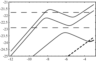
FIG. 1.: Gravitational wave amplitude of bursts emitted by cosmic string cusps (upper curves) and kinks (lower curve) in the LIGO/VIRGO frequency band, as a function of the parameter $\alpha=50\,G\,\mu$ (in a base-$10$ log-log plot). The upper curve assumes that the average number of cusps per loop oscillation is $c=1$. The middle curve assumes $c=0.1$. The lower curve gives the kink signal (assuming only one kink per loop). The horizontal dashed lines indicate the one sigma noise levels (after optimal filtering) of LIGO 1 (initial detector) and LIGO 2 (advanced configuration). The short-dashed line indicates the “confusion” amplitude noise of the stochastic GW background.

In Fig. 1 we plot (as solid lines) the logarithm of the GW burst amplitude, $\log_{10}(h^{\rm burst})$, as a function of $\log_{10}(\alpha)$ for: (i) cusps with $c=1$ (upper curve), (ii) cusps with $c=0.1$ (middle curve), and (iii) kinks with $k=1$ (lower curve). Fig. 1 uses the fiducial value $\dot{N}=1\,{\rm yr}^{-1}$, and gives the value of $h^{\rm cusp}$ or $h^{\rm kink}$ for a frequency $f=f_{c}=150\,{\rm Hz}$. As is discussed in the next Section, this central frequency is the optimal one for the detection of a $f^{-1/3}$-spectrum burst by LIGO. We indicate on the same plot (as horizontal dashed lines) the (one-sigma) noise levels $h^{\rm noise}$ of LIGO 1 (the initial detector), and LIGO 2 (its planned advanced configuration). The VIRGO detector has essentially the same noise level as LIGO 1 for the GW bursts considered here. We defer to the next Section the precise definition of these noise levels, as well as the meaning of the extra short-dashed line in the lower right corner of Fig. 1.

From Fig. 1 we see that the discovery potential of ground-based GW interferometric detectors is richer than hitherto envisaged, as it could detect (if $c\sim 1$) cosmic strings in the range $\alpha\,\raise 1.72218pt\hbox{$>$}\kern-6.99997pt\lower 2.6694pt\hbox{$\sim$}\,10^{-10}$, i.e. $G\,\mu\,\raise 1.72218pt\hbox{$>$}\kern-6.99997pt\lower 2.6694pt\hbox{$\sim$}\,10^{-12}$ (which corresponds to string symmetry breaking scales $\raise 1.72218pt\hbox{$>$}\kern-6.99997pt\lower 2.6694pt\hbox{$\sim$}\,10^{13}\,{\rm GeV}$). Even if $c\sim 0.1$, i.e if cusps are present only on $10\%$ of the loops in the network, which we deem quite plausible, (advanced) ground-based GW interferometric detectors might detect GW bursts from cusps in a wide range of values of $\alpha$. Let us also note that the value of $\alpha$ suggested by the (superconducting-) cosmic-string Gamma Ray Burst (GRB) model of Ref. [9], namely $\alpha\sim 10^{-8}$, nearly corresponds in Fig. 1 to a local maximum of the GW cusp amplitude. [This local maximum corresponds to $z_{m}\sim 1$. The local minimum on its right corresponds to $z\sim z_{\rm eq}$.] In view of the crudeness of our estimates, it is quite possible that LIGO 1/VIRGO might be sensitive enough to detect these GW bursts. Indeed, if one searches for GW bursts which are (nearly) coincident with (some) GRB the needed threshold for a convincing coincident detection is much closer to unity than in a blind search. Let us finally note that Fig. 1 indicates that (except if $k$ happens to be parametrically large) the kink bursts are too weak to provide an interesting source for LIGO/VIRGO.

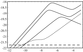
FIG. 2.: Gravitational wave amplitude of bursts emitted by cosmic string cusps (upper curves) and kinks (lower curve) in the LISA frequency band, as a function of the parameter $\alpha=50\,G\,\mu$ (in a base-$10$ log-log plot). The meaning of the three solid curves is as in Fig. 1. The short-dashed slanted curve indicates the confusion noise. The lower long-dashed line indicates the one sigma noise level (after optimal filtering) of LISA.

In Fig. 2, we do the same plot as Fig. 1 (still with $\dot{N}=1\,{\rm yr}^{-1}$), but with a central frequency $f=f_{c}=3.9\times 10^{-3}\,{\rm Hz}$ optimized for a detection by the planned space borne GW detector LISA. The meaning of the various curves is the same as in Fig. 1. The main differences with the previous plot are: (i) the signal strength, and the SNR, are typically much higher for LISA than for LIGO, so that LISA could be sensitive to even smaller values of $\alpha$ (down to $\alpha\simeq 10^{-11.6}$), (ii) LISA is very sensitive even to rare cusp events ($c=0.1$ or even smaller), (iii) LISA is, contrary to LIGO, sensitive to the kink bursts (which are believed to be ubiquitous), and (iv) though the GW burst signals still stand out well above the cusp-confusion background (discussed in the next Section), the latter is now higher than the (broad-band) detector noise in a wide range of values of $\alpha$. LISA is clearly a very sensitive probe of cosmic strings. We note again that a search in coincidence with GRB’s would ease detection.

VI Detection issues, confusion noise, pulsar timing experiments

A Signal to noise considerations

Let us first complete the explanation of Figs. 1 and 2 by discussing the choice of the central frequencies and the detector noise levels indicated there.

We recall that the optimal squared signal to noise ratio (SNR) for the detection of an incoming GW by correlation with a suitable bank of matched filters is given by

$$\rho^{2}=\left(\frac{S}{N}\right)^{2}=\int_{-\infty}^{+\infty}df\,\frac{|\widetilde{h}(f)|^{2}}{S_{n}(f)}=2\int_{0}^{+\infty}\frac{df}{f}\ \frac{|h(f)|^{2}}{(h_{n}(f))^{2}}\,.$$ (105)

Here $\widetilde{h}(f)$ is the Fourier transform of the (best) template (assumed to match the signal), $S_{n}(f)$ is the (two-sided) noise spectral density, and, as above, we introduce the logarithmic Fourier quantities $h(f)\equiv|f|\,\widetilde{h}(f)$, and $h_{n}(f)\equiv\sqrt{|f|\,S_{n}(f)}$. For cusp bursts (that we focus on) the optimal bank of filters (when neglecting the fine structure around the center of the cusp) is

$$h(f)=A\,|f|^{-1/3}\,e^{2\pi ift_{c}}\,,$$ (106)

and depends, besides the overall amplitude factor, on only one parameter: the arrival time $t_{c}$. We take the following model of the LIGO 1 (two sided) noise curve (see, e.g., [19]) (for $f$ above the seismic cut off $f_{s}\sim 40\,{\rm Hz}$)

$$S_{n}(f)=\frac{1}{2}\,S_{0}\left[2+2\left(\frac{f}{f_{0}}\right)^{2}+\left(\frac{f}{f_{0}}\right)^{-4}\right]\,.$$ (107)

Here, $S_{0}=1.47\times 10^{-46}\,{\rm Hz}^{-1}$ and $f_{0}=200\,{\rm Hz}$. [The form (107) is not really up to date, but it is sufficient for our present orientation estimate.] By inserting Eqs. (106) and (107) into Eq. (105) we get an explicit integral proportional to $\int(dx/x)(1/s(x))$ where $x\equiv f/f_{0}$ and $s(x)=x^{5/3}(2+2x^{2}+x^{-4})$. The minimum of the function $s(x)$ is located at $x_{m}=0.7483$, which corresponds to $f_{m}=x_{m}\,f_{0}=149.67\,{\rm Hz}$. Therefore LIGO 1 is optimally sensitive, for such signals, to the frequencies $f\sim f_{m}\sim 150\,{\rm Hz}$. [This value would also be approximately appropriate for kink signals, and also for the LIGO 2 noise curve.] Choosing $f_{c}=150\,{\rm Hz}$ as fiducial frequency, and reexpressing the full SNR (105) (including its overall amplitude factor $\propto\,|A|^{2}$) in terms not of $A$ but of $h(f_{c})$, one finds (after computing the integral) that

$$\rho\simeq\frac{|h(f_{c})|}{h_{n}^{\rm eff}}$$ (108)

with an “effective” noise level

$$h_{n}^{\rm eff}\simeq 1.7\times 10^{-22}\,.$$ (109)

The effective noise level (109) (which corresponds to a ${\rm SNR}=1$ for a matched filter detection) is what is called the “one sigma noise level” of LIGO 1 in Fig. 1. For LIGO 2 (advanced configuration) we estimated from noise curves, available on the LIGO web site, that, near $150\,{\rm Hz}$, the noise amplitude $h_{n}(f_{c})$ is a factor $\simeq 13.5$ smaller than for LIGO 1. This defines the lower dashed curve in Fig. 1.

We did a similar analysis for LISA. We used as (effective) noise curve the sum (with a factor $1/2$ included to take care of our using a two-sided spectral density)

$$S_{n}^{\rm tot}(f)=\frac{1}{2}\,[S_{h}^{\rm instr}(f)+S_{h}^{\rm conf}(f)]\,,$$ (110)

where $S_{h}^{\rm instr}$ is a recent estimate of the instrumental contribution to the noise [21]

$$S_{h}^{\rm instr}(f)\simeq 2.13\times 10^{-41}\left[1+\left(\frac{f_{a}}{f}\right)^{4}\right]\sqrt{1+\left(\frac{f}{f_{p}}\right)^{4}}\,,$$ (111)

where $f_{a}=2.76\times 10^{-3}\,{\rm Hz}$, $f_{p}=9.55\times 10^{-3}\,{\rm Hz}$, and where $S_{h}^{\rm conf}(f)$ is the “binary confusion noise”, as estimated in Ref. [22]. Again the optimal frequency is fixed by considering the minimum of $h_{n}^{2}(f)/|h(f)|^{2}\propto f^{5/3}\,S_{n}^{\rm tot}(f)$, which occurs at $f_{m}=10^{-2.4113}\,{\rm Hz}=3.879\times 10^{-3}\,{\rm Hz}$. And again the “one sigma” effective noise level (dashed horizontal line in Fig. 2) is defined by (108), with the result: $h_{n}^{\rm eff}=1.815\times 10^{-22}$.

Let us also briefly mention the problem of “thresholds”, i.e. the minimum value of the SNR, say $\rho_{0}$, needed to distinguish, with enough confidence, a real signal from a statistical fluctuation of the instrumental noise. Assuming, for simplicity, Gaussian instrumental noise, the probability that the template-filtered detector output exceed a certain level $\rho_{0}$ of SNR is given by the complementary error function

$$p(\rho>\rho_{0})=\left(\frac{2}{\pi}\right)^{\frac{1}{2}}\int_{\rho_{0}}^{\infty}d\rho\,e^{-\frac{1}{2}\rho^{2}}\simeq\left(\frac{2}{\pi}\right)^{\frac{1}{2}}(\rho_{0}-\rho_{0}^{3})\,e^{-\frac{1}{2}\rho_{0}^{2}}\,.$$ (112)

We are interested in the situation where two independent detectors (either two ground based interferometers, or the two, partly independent, subinterferometers of LISA) find a coincidence, after having made $N$ observations during the year. In our case, each template contains only the arrival time as essential free parameter. Therefore, the number of observations, assuming a blind search, in one year is $N\sim(1\,{\rm yr})/\tau=(10^{7.5}\,{\rm s})/\tau$ where $\tau\sim f_{c}^{-1}$ is the characteristic time between two decorrelated successive observations. Assuming the same noise level in each detector, the looked for threshold $\rho_{0}$ can be defined by equalling the product of two probabilities equal to (112) (one for each detector), i.e. the square of (112), to $1/N$. When $\tau\sim 10^{-2}\,{\rm s}$ (as appropriate to LIGO) this yields $\rho_{0}\simeq 4.3$, while when $\tau\sim 3\times 10^{2}\,{\rm s}$ (LISA) this yields $\rho_{0}\simeq 3.0$. Note, however, that the model of [9] suggests that GWB’s may be associated to Gamma Ray Bursts. The threshold for a search in near coincidence with GRB’s is somewhat lower, because of the smaller number of trial observations $N$.

B Confusion noise due to gravitational waves from a string network

The realization that the stochastic ensemble of GW’s generated by a cosmological network of oscillating loops is strongly non Gaussian, and includes occasional sharp bursts, raises the following issues, of crucial importance for the detection strategies: (i) Can one split this stochastic ensemble of GW’s into a (strongly non Gaussian, but plausibly nearly Poissonian) “burst” part (best detected by a matched filter approach), and a (nearly Gaussian) “background” (best detected by the usual strategies discussed for Gaussian stochastic backgrounds)?, and (ii) What is the relation of this split to previous estimates of the “stochastic” string-generated background of GW’s [2, 3, 4, 5, 6, 7], and how does it affect the interpretation of the famous pulsar timing constraint [23]?

Our proposal is, for each detector with characteristic (optimal) detection frequency $f_{c}$, and for each GW amplitude level, to define the borderline between occasional, individual sharp bursts, and a nearly Gaussian background by counting the average number of bursts of given amplitude which arrive within a characteristic time $t_{c}=f_{c}^{-1}$. In other words, we define a nearly Gaussian background by considering the confusion noise generated by the overlap of more than one (and generally many) bursts which arrive within a time smaller than the considered characteristic inverse frequency. A technical way of justifying this (physically intuitive) consideration is the following.

Let us write, in the time domain, our stochastic ensemble of GW’s from a string network as

$$h(t)=\sum_{n}h(t-t_{n},z_{n},p_{n})\,.$$ (113)

Here, the (somewhat symbolic) sum runs over waveforms arriving at time $t_{n}$ and emitted from a string loop at redshift $z_{n}$, with other string parameters (length, orientation,$\ldots$) being denoted $p_{n}$. The (logarithmic) Fourier transform of (113) reads

$$h(f)\equiv|f|\,\widetilde{h}(f)=\sum_{n}e^{2\pi ift_{n}}\,h(f,z_{n},p_{n})\,.$$ (114)

Let us now recall that the spectral noise density of a stochastic ensemble of signals is defined by $\langle\widetilde{h}^{*}(f)\,\widetilde{h}(f^{\prime})\rangle=\delta(f-f^{\prime})\,S_{h}(f)$ where $\langle\ \rangle$ denotes an ensemble average, a tilde the usual Fourier transform and a star, complex conjugation. Defining the (total) root mean square (rms) GW amplitude $h_{\rm rms}(f)$ (with the same dimension as $h(t)$, i.e. dimensionless) by $h_{\rm rms}^{2}(f)\equiv|f|\,S_{h}(f)$, the above definition of $S_{h}(f)$ becomes, in terms of the more convenient logarithmic Fourier quantities

$$\langle h^{*}(f)\,h(f^{\prime})\rangle=|f|\,\delta(f-f^{\prime})\,h_{\rm rms}^{2}(f)\,.$$ (115)

When we take the (formal) limit $f^{\prime}\rightarrow f$, the delta function $\delta(f-f^{\prime})=\int dt\exp(2\pi i(f-f^{\prime})t)$ becomes a (formally infinite) total time interval $T=\int dt$

$$\langle h^{*}(f)\,h(f)\rangle=|f|\,T\,h_{\rm rms}^{2}(f)\,.$$ (116)

Let us now compute the quantity $\langle h^{*}(f)\,h(f)\rangle$ by squaring the expression (114). Before taking the ensemble average, we get a double sum over $n$ and $n^{\prime}$ involving phase factors $e^{2\pi if(t_{n}-t_{n^{\prime}})}$ in addition to the other phase factors hidden in the dependence on the other parameters. If we assume (as usual) that such phase factors are random and average to zero (except when $n=n^{\prime}$) we get

$$\langle h^{*}(f)\,h(f)\rangle=\sum_{n}|h(f,z_{n},p_{n})|^{2}\,.$$ (117)

Within our simplified approach to the string network, we assume that the GW amplitudes differ only by their redshift of emission $z_{n}$. The sum over $z_{n}$ (within some octave around $z$) then counts the number of signals coming from $dz/z$ during the total time $T$. In terms of our previously introduced differential rate of occurrence $\dot{N}(f,z)$ this yields simply

$$\langle h^{*}(f)\,h(f)\rangle=T\int\frac{dz}{z}\ \dot{N}(f,z)\ h^{2}(f,z)\,.$$ (118)

Identifying this result with (116) we finally get

$$h_{\rm rms}^{2}(f)=\int\frac{dz}{z}\ n(f,z)\,h^{2}(f,z)\,,$$ (119)

where we introduced the shorthand notation

$$n(f,z)\equiv\frac{\dot{N}(f,z)}{|f|}=\frac{1}{|f|}\ \frac{d\,\dot{N}}{d\,\ln\,z}\,.$$ (120)

This derivation has achieved two aims: (1) it gives us an explicit expression, (119), (computable in terms of quantities that we calculated above) for the usually considered rms GW background generated by a string network, and (2) it shows (by comparison to the usual rms value of a sum of $n$ independent random variables with the same variance) that the quantity $n(f,z)$, Eq. (120), gives, in a technically precise sense, the (effective) number, within an octave of frequency around $f$, of random GW bursts generated at redshift $z$, and therefore of amplitude $h(f,z)$, which contribute to $h_{\rm rms}^{2}$. The latter result leads us to split the ensemble of GW signals in two sets: (i) the set of rare, non overlapping bursts such that $n(f,z)<1$, and (ii) the set of frequent, overlapping bursts, such that $n(f,z)>1$. The rare, non overlapping bursts contribute to $h_{\rm rms}^{2}(f)$ only if one considers integration times $T\gg(\dot{N}(f,z))^{-1}\equiv(n(f,z)\,|f|)^{-1}>|f|^{-1}$. Therefore, if we are interested in detection issues involving a detector with a certain characteristic bandwidth $\sim f_{c}$, and a corresponding integration time $T_{c}\sim f_{c}^{-1}$, all the bursts such that $n(f_{c},z)<1$ should be considered as randomly occurring separate burst events, and the magnitude of these occasional events should not be compared to the full $h_{\rm rms}^{2}(f_{c})$ of Eq. (119) but only to the “confusion” noise defined by restricting the integral (119) to the overlapping events, $n(f_{c},z)>1$. [By the central limit theorem, applicable when $n(f_{c},z)\gg 1$, this confusion noise can be considered as being nearly Gaussian.] Therefore we define

$$h_{\rm confusion}^{2}(f)\equiv\int\frac{dz}{z}\ n(f,z)\,h^{2}(f,z)\,\Theta(n(f,z)-1)\,.$$ (121)

We conclude that the relevant background that individual cusp or kink bursts should exceed to be detectable by LIGO (central frequency $f_{c}=150\,{\rm Hz}$) or LISA ($f_{c}=3.88\times 10^{-3}\,{\rm Hz}$) is not $h_{\rm rms}^{2}(f_{c})$, Eq. (119), but only $h_{\rm confusion}^{2}(f_{c})$, Eq. (121). The short dashed lines in Fig. 1 and Fig. 2 plot precisely the quantity (121), for the $c=1$ cusp background, i.e. for $h(f,z)$ given by (84), and $\dot{N}(f,z)$ given by Eq. (91) (with $c=1$). This shows that in the LIGO or LISA bandwidths the individual bursts occurring once per year stand out clearly above the relevant confusion noise.

C Rare bursts, confusion noise and pulsar timing experiments

Our finding that the stochastic ensemble of string-generated GW’s is not Gaussian, but can be viewed as the superposition of occasional bursts on top of a nearly Gaussian “confusion” background leads us to reexamine the pulsar timing experiments [23] and their use as constraints on the string tension $G\,\mu$. Let us take as characteristic frequency of the pulsar timing experiments the frequency $f_{c}^{\rm psr}=1/(7\,{\rm yr})=10^{-8.35}\,{\rm Hz}$ which roughly corresponds to the optimal sensitivity of the data of Refs. [23]. To get a first idea of the situation, let us start by considering the fiducial value $\alpha_{\rm fid}=10^{-4}$ corresponding to $G\,\mu\sim\alpha/50=2\times 10^{-6}$, i.e. the traditionally considered type of string tensions (which can naturally come from Grand Unified Theories (GUT) and which is most relevant for large scale structure formation). We can compare three different GW amplitudes of relevance for the pulsar experiment: (i) the amplitude of individual bursts having a recurrence rate $f_{c}^{\rm psr}=1/(7\,{\rm yr})$ (instead of the $1/{\rm yr}$ recurrence rate considered above for LIGO or LISA), (ii) the rms amplitude of our confusion background (121), and (iii) the rms amplitude of the usually discussed full integral (119) which includes both rare bursts and overlapping ones. We find

$$h_{1/7}^{\rm cusp}(\alpha_{\rm fid},f_{c}^{\rm psr})=0.503\times 10^{-13}\,,$$ (123)

$$h_{\rm confusion}(\alpha_{\rm fid},f_{c}^{\rm psr})=1.01\times 10^{-13}\,,$$ (124)

$$h_{\rm rms}^{\rm usual}(\alpha_{\rm fid},f_{c}^{\rm psr})=2.30\times 10^{-13}\,.$$ (125)

In computing the integrals (119) and (121) we have here used (for better accuracy) an improved estimate of the space density of loops, $n_{\ell}$, Eq. (75). Indeed, numerical simulations indicate that, beyond the scaling $n_{\ell}\sim\alpha^{-1}\,t^{-3}$ one must add an extra factor related to the parameter characterizing the density of long strings. This factor is different in the radiation era and in the matter era. In the notation of [1] this extra factor is $\sim 0.4\,\zeta_{r}\sim 10$ in the radiation era, and is $\sim 0.12\,\zeta_{m}\sim 1$ during the matter era. In other words, a better estimate of $n_{\ell}$ is obtained by multiplying the estimate (75) by the function

$$C(z)=1+9z/(z+z_{\rm eq})$$ (126)

which interpolates between 1 in the matter era and 10 in the radiation era.

Note that, in terms of the contribution (per frequency octave) of GW’s to the present energy density, $\rho_{\rm GW}(f)\sim(2\pi f\,h(f))^{2}/(16\pi G)\sim(\pi/4G)\,f^{2}\,h^{2}$, or, better, of their fractional contribution to the closure density,

$$\Omega_{\rm gw}(f)\equiv\frac{\rho_{\rm GW}(f)}{\rho_{c}}=6\pi\,G\,t_{0}^{2}\,\rho_{\rm GW}\sim\frac{3\pi^{2}}{2}\ (f\,t_{0})^{2}\,h_{\rm rms}^{2}(f)\,,$$ (127)

the results (VI C) yield

$$\Omega_{\rm gw}^{\rm confusion}(\alpha_{\rm fid},f_{c}^{\rm psr})=2.99\times 10^{-7}\,,$$ (128)

$$\Omega_{\rm gw\,rms}^{\rm usual}(\alpha_{\rm fid},f_{c}^{\rm psr})=1.57\times 10^{-6}\,.$$ (129)

The usually considered $\Omega_{\rm gw}$ is 5.25 times larger than the physically meaningful confusion noise! This large discrepancy comes from the fact that $\Omega_{\rm gw}^{\rm usual}$ includes the time-average contribution of rare, intense bursts, which are in general, not relevant for a pulsar experiment (if they are so rare that they do not occur during the actual duration of the experiment).

From this consideration, it would seem to follow that the usual way to use pulsar data to set limits on $G\,\mu$ (i.e. the comparison between the theoretically predicted $\Omega_{\rm gw\,rms}^{\rm usual}(\alpha,f)$ and the observational constraint on a Gaussian $\Omega_{\rm gw}^{\rm obs}(f)$) is seriously affected by the present work. It would also seem that the correct way to set limits on $G\mu$ from pulsar data consists simply in replacing $\Omega_{\rm gw\,rms}^{\rm usual}$ by our new, significantly smaller, $\Omega_{\rm gw}^{\rm confusion}$. Then the value (128) suggests that even cusp- (rather than kink-) dominated backgrounds, with $c=1$ (as the one considered in the equations above) generated by string tensions $G\,\mu$ of order of $10^{-6}$ might be compatible with pulsar constraints at the $\Omega_{\rm gw}^{\rm obs}\,\raise 1.72218pt\hbox{$<$}\kern-8.00003pt\lower 2.6694pt\hbox{$\sim$}\,10^{-7}$ level. [In view of the crudeness of our estimates we shall not try here to give any precise limit on $G\,\mu$ from $\Omega_{\rm gw}^{\rm obs}$.]

However, Eqs. (VI C) show that the situation is actually somewhat more complex than that. Indeed, Eq. (123) shows that the (observationally relevant) $1/(7\,{\rm yr})$ bursts have an amplitude comparable to the full confusion noise (which sums many overlapping, small signals). [This comes from the fact that the confusion integral (121) is dominated by its lower limit.] Therefore a significant part of the difference between $h_{\rm confusion}$ and $h_{\rm usual}$ comes from not very intense, but not very rare bursts. [Note, however, that the dominant contribution in $h_{\rm rms}^{\rm usual}$ comes from the very intense, very rare bursts, with recurrence time $\gg 7{\rm yr}$.] In other words, Eqs. (VI C) show that, within the frequency bandwidth $\sim f_{c}^{\rm psr}$ relevant for pulsar timing, the GW signal $h(f)$ is a complicated superposition of a nearly Gaussian noise (of variance $h_{\rm confusion}^{2}$) and of a small number of occasional random bursts, occurring on the $(f_{c}^{\rm psr})^{-1}$ time scale and of amplitude comparable to $h_{\rm confusion}(f_{c})$. In addition, there might also occur (on longer time scales) some larger bursts. This situation shows that one needs to reanalyze from scratch the pulsar limits on $G\,\mu$ by dealing explicitly with the statistical properties of such a complicated mix of signals, i.e. by tackling seriously the strongly non Gaussian nature (involving an important quasi-Poissonian component) of $h(f)$ within the pulsar timing bandwidth. Until such an analysis, using our new results on the nature of the string GW background, is performed one cannot draw secure limits on $G\,\mu$ from pulsar observations. We expect, however, that the result of such an analysis will be, to a good approximation, equivalent to replacing $\Omega_{\rm gw}^{\rm usual}$ by our new $\Omega_{\rm gw}^{\rm confusion}$ (which is about five times smaller than $\Omega_{\rm gw}^{\rm usual}$ when $G\mu=2\times 10^{-6}$, and about four times smaller when $G\mu=10^{-6}$). In particular, we expect that our results make a GUT-like value $G\mu\sim 10^{-6}$ now compatible (even with many cuspy loops) with present pulsar data.

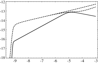
FIG. 3.: Usual rms noise (upper short-dashed curve), confusion noise (lower short-dashed curve) and burst GW amplitude (solid line) emitted by cosmic string cusps, in the frequency band relevant for pulsar timing observations $(f_{c}=\dot{N}=1/(7\,{\rm yr}))$. Here, we assumed $c=1$ and included the factor (126) in the spatial density of loops.

Leaving to future work such an analysis, we content ourselves by comparing in Fig. 3 the variation with $\alpha$ of the cusp burst signal (for $c=1$ and $\dot{N}=1/(7\,{\rm yr})$), the confusion GW amplitude $h_{\rm confusion}(f_{c}^{\rm psr})$ ($f_{c}^{\rm psr}=1/(7\,{\rm yr})$), and the usually considered total rms amplitude $h_{\rm rms}^{\rm usual}(f_{c}^{\rm psr})$. Contrary to what happened in Fig. 1 and Fig. 2, we see now that the burst signal and the confusion signal are of comparable orders of magnitude in a wide range of values of $\alpha=50\,G\,\mu$. Note also that $h_{\rm rms}^{\rm usual}$ is a significant overestimate of $h_{\rm confusion}$ when $\alpha\raise 1.72218pt\hbox{$>$}\kern-6.99997pt\lower 2.6694pt\hbox{$\sim$}5\times 10^{-6}$, i.e. $G\mu\raise 1.72218pt\hbox{$>$}\kern-6.99997pt\lower 2.6694pt\hbox{$\sim$}10^{-7}$, which includes the GUT case which has been traditionally of most interest for cosmic string research. In view of the subtlety we just mentionned concerning the data analysis of pulsar experiments we did not indicate in Fig. 3 a precise “one sigma” level for the sensitivity of the pulsar experiment. [A rough guess, using Eq. (127) with $\Omega_{\rm gw}^{\rm psr}\sim 10^{-7}$ is $h^{\rm psr}\sim 0.5\times 10^{-13}$.]

Switching from a defensive attitude (pulsar limits on $G\mu$) to an optimistic one (detection of GW by pulsar experiments), and forgetting for a moment the subtlety of the fact that $h^{\rm burst}\sim h^{\rm confusion}$ (i.e. assuming that $h^{\rm confusion}$ gives a good first estimate of the GW amplitude to be compared to the timing precision of pulsar experiments), it is striking to notice on Fig. 3 that $h^{\rm confusion}$ is a very flat function of $\alpha$, so that a modest improvement in the sensitivity of pulsar experiments (due either to a longer time span or to the discovery of an intrinsically more stable pulsar) might allow one to detect the confusion noise coming from a string network down to $\alpha\sim 10^{-9}$ (i.e. $G\,\mu\sim 10^{-11}$). Evidently one should keep in mind that Fig. 3 is drawn for an average cusp number $c=1$. Assuming a smaller value of $c$, or even $c=0$ and considering only the smaller kink signals, will make it much more difficult for pulsar experiments to probe the existence of cosmic strings.

VII Conclusions

We have studied in detail the amplitude, frequency spectrum, waveform and rate of occurrence of the high-frequency gravitational wave (GW) bursts emitted at cusps and kinks of a cosmological network of oscillating loops. Our main tool in studying the waveform has been the factorization (23) of the Fourier transform of the emitted GW amplitude. This factorization allowed us to conveniently extract from the waveform its physically meaningful, gauge-invariant content. [This is why our waveforms differ from previous results [13, 11] which did not notice the gauge nature of the leading terms.] In the time domain these waveforms correspond to power-law “spikes” $\propto|t-t_{c}|^{\beta}$ ($\beta=\frac{1}{3}$ for cusps; and $\beta=\frac{2}{3}$ for kinks) of linearly polarized GW’s, with some smoothing of the center of the spike on time scales $|t-t_{c}|\sim\theta^{3}\,T_{\ell}$, where $T_{\ell}=\ell/2$ is the loop oscillation period and where $\theta$ is the misalignement between the center of the beam and the direction of emission.

We estimated the rate of occurrence and the distribution in amplitude of the GW bursts emitted at cusps and kinks by using a simple model for the cosmic string network. When comparing our results with observations, one should keep in mind the simplifying assumptions involved in our model: (i) All loops born at time $t$ were assumed to have length $\ell\sim\alpha\,t$ with $\alpha\sim\Gamma\,G\,\mu$ and $\Gamma\sim 50$. It is possible, however, that the loops have a broad length distribution $n(\ell,t)$ and that the parameter $\alpha$ characterizing the typical loop length be in the range $\Gamma\,G\,\mu<\alpha\ \raise 1.72218pt\hbox{$<$}\kern-8.00003pt\lower 2.6694pt\hbox{$\sim$}\ 10^{-3}$. (ii) We have also assumed that the loops are characterized by a single length scale, with no wiggliness on smaller scales. Short-wavelength wiggles on scales $\ll\Gamma\,G\,\mu\,t$ are damped by gravitational back-reaction but some residual wiggliness may survive, thereby modifying the amplitude and the angular distribution of the GW bursts from cusps and kinks. (iii) In many of our estimates we assumed the simple, uniform estimate (75) for the space density of loops. This estimate is probably accurate in the matter era but is expected to be too small by a factor $\sim 10$ in the radiation era [1]. In Section VI where the contribution to the confusion background of the radiation era was crucial we corrected the estimate (75) by including the redshift-dependent factor (126). (iv) Finally, we disregarded the possibility of a nonzero cosmological constant which would introduce some quantitative changes in our estimates. As a general comment, let us recall that, though we tried to keep the important “$2\pi$ factors”, our estimates have systematically neglected factors of order unity.

In our view the most important astrophysical results of the present investigation are the following: (1) the clear recognition of the strongly non Gaussian nature of the string-generated GW background. The slow decrease with frequency of the GW burst signals means that there are occasional sharp bursts that stand above the “confusion” GW noise made of the superposition of the overlapping bursts. (2) GW bursts from cusps might be detectable by the planned GW detectors LIGO/VIRGO and LISA for a wide range of string tensions even if the average number of cusps per string oscillation is only $10\%$. In spite of the argument [11] that string reconnection can inhibit cusps (which are generic for smooth loops [10]), we find it plausible that $10\%$ or at least a few $\%$ of the loops in the network will feature cusps. In view of the crucial importance of the average number of cusps for detection by LIGO we recommend that new simulations be performed to determine this quantity. (3) Even if the number of cusps turns out to be very small, our estimate of the GW amplitude emitted by the ubiquitous kinks show that the space borne GW detector LISA has the potential of detecting GW bursts from kinks in a wide range of string tensions. (4) Finally, we show the need of a reanalysis of the constraints on $G\,\mu$ derived from pulsar timing data. Indeed, for such low frequencies the usual estimate, Eq. (119), of the GW stochastic background (which neglects its non Gaussianity) seems to be quite inadequate because it averages on very rare, intense bursts. We have introduced a new, more relevant quantity, the confusion noise, Eq. (121), which averages only over the overlapping bursts. In the first approximation, we expect that the usually derived pulsar timing data limit on a Gaussian stochastic background (often expressed as a limit $\Omega_{\rm gw\,PSR}^{\rm Gaussian}\raise 1.72218pt\hbox{$<$}\kern-8.00003pt\lower 2.6694pt\hbox{$\sim$}10^{-7}$) will entail essentially the same limit on the confusion part, Eq.(121), of the GW stochastic background, i.e. we expect that the real pulsar limit on $G\mu$ will be the weaker constraint $\Omega_{\rm gw}^{\rm confusion}(G\mu)<\Omega_{\rm gw\,PSR}^{\rm Gaussian}$. Our rather crude approximations do not allow us to transform this relaxed limit in a precise limit on $G\mu$. However, we expect that our results render a GUT-like value $G\mu\sim 10^{-6}$ compatible with pulsar data, even if $c\sim 1$ (and probably easily compatible with $G\mu\sim 10^{-6}$ if $c$ is $10\%$ or less). However, we emphasized that there are still occasional bursts that complicate the analysis and call for an improved treatment. Until such a careful analysis is done, together with a precise estimate of the number of cusps in a string network, one cannot use pulsar data to set precise limits on $G\,\mu$.

REFERENCES

• [1] For a review of string properties and evolution, and references to original work, see, e.g., A. Vilenkin and E.P.S. Shellard, Cosmic strings and other topological defects, Cambridge University Press, Cambridge, 2000 (updated paperback edition).
• [2] A. Vilenkin, Phys. Lett. 107B, 47 (1981).
• [3] C.J. Hogan and M.J. Rees, Nature 311, 109 (1984).
• [4] T. Vachaspati and A. Vilenkin, Phys. Rev. D31, 3052 (1985).
• [5] D. Bennett and F. Bouchet, Phys. Rev. Lett, 60, 257 (1988).
• [6] R.R. Caldwell and B. Allen, Phys. Rev. D45, 3447 (1992).
• [7] R.R. Caldwell, R.A. Battye and E.P.S.Shellard, Phys. Rev. D54, 7146 (1996).
• [8] T. Damour and A. Vilenkin, Phys. Rev. Lett. 85, 3761 (2000).
• [9] V. Berezinsky, B. Hnatyk and A. Vilenkin, astro-ph/0001213.
• [10] N.G. Turok, Nucl. Phys. B242, 520 (1984).
• [11] D. Garfinkle and T. Vachaspati, Phys. Rev. D37, 257 (1988).
• [12] This formula, valid for any, possibly relativistic, source at the linearized approximation is a standard result, given, e.g., in the book of S. Weinberg, Gravitation and Cosmology (Wiley, New York, 1972). We rederived it from scratch both to establish our notation in detail and because it is underused, for waveform calculations, in the cosmic-string literature.
• [13] T. Vachaspati, Phys. Rev. D35, 1767 (1987).
• [14] C.J. Burden, Phys. Lett 164B, 277 (1985).
• [15] D. Garfinkle and T. Vachaspati, Phys. Rev. D36, 2229 (1987).
• [16] B. Allen and E.P.S. Shellard, Phys. Rev. D45, 1898 (1992).
• [17] B. Allen and A. C. Ottewill, Phys. Rev. D63, 063507 (2001).
• [18] T.W.B. Kibble and N.G. Turok, Phys. Lett. 116B, 141 (1982).
• [19] T. Damour, B.R. Iyer and B.S. Sathyaprakash, Phys. Rev. D62, 684036 (2000).
• [20] T. Damour and A. Vilenkin, Phys. Rev. Lett. 78, 2288 (1997).
• [21] R. Schilling, private communication.
• [22] P.L. Bender and D. Hils, Class. Quant. Grav. 14, 1439 (1997).
• [23] V.M. Kaspi, J.H. Taylor and M.F. Dewey, Phys. Rev. 53, 3468 (1996).