The Gravitational Wave Background from Cosmological Compact Binaries

Abstract

We use a population synthesis approach to characterise, as a function of cosmic time, the extragalactic close binary population descended from stars of low to intermediate initial mass. The unresolved gravitational wave (GW) background due to these systems is calculated for the 0.1–10 mHz frequency band of the planned Laser Interferometer Space Antenna (LISA). This background is found to be dominated by emission from close white dwarf–white dwarf pairs. The spectral shape can be understood in terms of some simple analytic arguments. To quantify the astrophysical uncertainties, we construct a range of evolutionary models which produce populations consistent with Galactic observations of close WD–WD binaries. The models differ in binary evolution prescriptions as well as initial parameter distributions and cosmic star formation histories. We compare the resulting background spectra, whose shapes are found to be insensitive to the model chosen, and different to those found recently by Schneider et al. (2001). From this set of models, we constrain the amplitude of the extragalactic background to be $1\times 10^{-12}\la\Omega_{\rm{gw}}\rm{(1~{}mHz)}\la 6\times 10^{-12}$, in terms of $\Omega_{\rm{gw}}(f)$, the fraction of closure density received in gravitational waves in the logarithmic frequency interval around $f$.

1 Introduction

Except at very low radio frequencies, most electromagnetic telescopes have good angular rejection, so that faint sources and backgrounds can be seen by looking between bright sources. In contrast all currently implemented gravitational wave detectors, and most of those envisaged for the future, simultaneously respond to sources all over the sky, modified only by a beam pattern of typically quadrupole form. It is therefore important to understand the brightness of the gravitational wave sky, since this will limit the ultimate sensitivity attainable in gravitational wave astronomy. One immediate pressure to understand this background comes from the need to set design requirements for the ESA/NASA Laser Interferometer Space Antenna (LISA) mission (LISA mission documents and status may be found at http://lisa.jpl.nasa.gov/ and http://sci.esa.int/home/lisa/).

In this paper, we attempt to predict the gravitational wave background produced by all the binary stars in the universe, excluding neutron stars and black holes. This is believed to be the principal source of gravitational wave background in the frequency range $10^{-5}<f<10^{-1}$ Hz. Below $10^{-5}$ Hz, the background is probably dominated by merging supermassive black holes, and above $10^{-1}$ Hz, it is probably dominated by merging neutron stars and stellar mass black holes (whose complicated and poorly understood formation histories and birth velocities make predictions more uncertain, cf. Belczynski, Kalogera & Bulik 2002).

Besides the extragalactic background, there is also a Galactic background produced by the binary stars in our Milky Way (Evans, Iben & Smarr 1987; Hils, Bender & Webbink 1990; Nelemans, Yungelson & Portegies Zwart 2001c). Although the Galactic background is many times larger in amplitude than both the extragalactic background and LISA’s design sensitivity, the individual binaries contributing to it can be (spectrally) resolved and removed at frequencies above $\sim 3\times 10^{-3}$ Hz (Cornish & Larson, 2002). Below this frequency they cannot be removed (at least in a mission of reasonable lifetime $\sim 3$ years), but the unresolved Galactic background will be quite anisotropic. As the detector beam pattern rotates about the sky, the Galactic background will thus be modulated, while the isotropic (or nearly so; see Kosenko & Postnov 2000) distant extragalactic background will not. Modelling of the angular distribution of the Galactic background using both a priori models and the observed distribution of higher frequency resolved sources will thus allow the Galactic background to be subtracted to some precision (Giampieri & Polnarev 1997). In addition, there will be anisotropies due to the distribution of local galaxies, at the level of 10 per cent of the distant extragalactic background from the LMC, and at the per cent level from M31 or the Virgo cluster (see also Lipunov et al. 1995).

The immediate motivation for this work is a design issue for LISA. One of LISA’s major science goals (see the LISA Science Requirements document at http://www.tapir.caltech.edu/listwg1/) is the detection of gravitational waves from compact objects spiralling into supermassive black holes (Finn & Thorne 2000; Hils & Bender 1995), since these can provide precision tests of strong field relativity and the no-hair theorem (Hughes, 2001). However, these signals are weak, and their templates not yet fully understood. It has thus been proposed that LISA should be designed with somewhat greater sensitivity to increase the probability that these signals are detected. However, this would be pointless if the principal background were cosmological rather than instrumental. As we shall see (Fig. 16), we find that this is most probably almost, but not quite the case at the relevant frequencies ($4-10$ mHz). So there would be a point to increasing LISA’s sensitivity in the $4-10$ mHz range, but not to increasing it by more than a factor of 3 in gravitational wave amplitude $h$ (9 in $\Omega\propto f^{2}h^{2}$).

A second motivation for this work comes from the fact that this background is an astrophysical foreground to searches (both with LISA and with future detectors with extended frequency range and sensitivity) for backgrounds produced in the very early universe. Gravitational waves from bubble walls and turbulence following the electroweak phase transition are expected to be in the LISA frequency band, with amplitude that could be well above LISA instrumental sensitivity (Kamionkowski, Kosowski & Turner 1994; Kosowsky, Mack & Kahniashvili 2002; Apreda et al. 2002). Another potential source of isotropic gravitational waves in the LISA band are those produced when dimensions beyond the familiar four compactified, which occurred when the universe had temperature $kT>$TeV (Hogan, 2000).

Note that detection of a gravitational wave background can possibly be made even if it is considerably below the noise limit of the LISA detectors shown in our Fig. 16. This can be done by comparing the signals from Michelson beam combinations (sensitive to instrument noise and gravitational waves) with Sagnac beam combinations (sensitive to instrument noise, but insensitive to gravitational waves), thus calibrating the instrumental noise —cf. Tinto, Armstrong & Estabrook (2001), Hogan & Bender (2001).

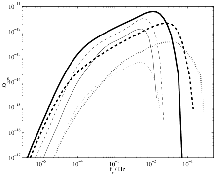
Figure 8: The background received from different WD–WD pairings, for Model A. From top to bottom at 1 mHz: thick solid line: CO–CO, thin dashed line: He–CO, thin solid line: He–He, thick dashed line: CO–ONe, thick dotted line: ONe–ONe, thin dotted line: He–ONe.

Gravitational waves are the only directly detectable relic of inflation in the early universe, and their detection over a range of frequencies would provide a valuable test of models of inflation (Turner, 1997). It has been proposed that advanced space-based gravitational wave detectors might search for the background of gravitational waves from inflation. The gravitational waves from slow-roll inflation models contribute to the critical density in the universe $\Omega_{\rm{gw}}<10^{-15}$ per octave of frequency. We shall see (Fig. 8, 17) that the gravitational wave background from cosmological binaries makes such detection impractical except at frequencies below $10^{-5}$ Hz (where supermassive black holes continue to make it impossible), or above $0.1$ Hz.

A third motivation is that a detection of the extragalactic binary background, e.g. by LISA, would set an independent (and unaffected by dust extinction) constraint on a combination of the star formation history of the universe and binary star evolution.

There have been previous estimates of the extragalactic binary background. Hils, Bender & Webbink (1990) made detailed estimates of the Galactic binary background, and estimated that the extragalactic background from close double white dwarf pairs should be about 2 per cent (in flux or $\Omega$ units) of the Galactic background. This estimate was refined, using more modern star formation histories, by Kosenko & Postnov (1998), who found instead a level of $\sim$10 per cent. Schneider et al. (2001) used a descendant of the Utrecht population synthesis code to estimate the extragalactic binary background as a function of frequency, and claimed that the background should have a large peak at $\sim 3\times 10^{-5}$ Hz, just below the frequency at which typical binaries have a lifetime that equals the age of the Universe.

We have followed the spirit of this previous work, but with an independent binary population synthesis code. More importantly, we have devoted much effort to the normalisation of the background, to understanding the contributions of different types of binaries and their formation pathways to the background, and to estimating the uncertainties in all of these, so that we can have a better idea of the sources and level of uncertainty in the predicted background.

The paper is organised as follows: In section 2, we describe the gravitational wave (GW) emission from a binary system, then in section 3 we outline the main evolutionary pathways to the close double degenerate (DD) stage, which we shall see is the dominant source of GW background in the LISA band. In section 4, we use the preceding sections to make some simple analytic arguments about the nature of DD inspiral spectra. We describe the use of the bse code in our population synthesis, in section 5, then go on to construct a set of synthesis models whose results we test against the observed Galactic DD population. We also motivate some modifications made to the prescription for the evolution of AM CVn stars in the bse code. In section 6, we present the cosmological integrals used in the code, along with the cosmic star formation history and overall normalisation chosen. Section 7 is devoted to a discussion of the GW background spectra produced by our code, in terms of the systems contributing to the background and the progenitors of these sources. We also discuss the differences between our population synthesis models. In section 8, we place limits on the maximum and minimum expected background signals, and compare these with the LISA sensitivity and in section 9 with previous work. In section 10 we summarise and conclude.

2 Gravitational waves from a binary system

A binary system of stars in circular orbit with masses $M_{1}$ and $M_{2}$ and orbital separation $a$ emits gravitational radiation, at the expense of its orbital energy, at a rate given by (Peters & Mathews, 1963)

$$L_{\rm{circ}} = \frac{32}{5}\frac{G^{4}}{c^{5}}\frac{(M_{1}M_{2})^{2}(M_{1}+M_{2})}{a^{5}}$$ (1)

$$\simeq 1.0\times 10^{32}\frac{(M_{1}^{\prime}M_{2}^{\prime})^{2}(M_{1}^{\prime}+M_{2}^{\prime})}{(a^{\prime})^{5}}\textrm{ erg s}^{-1},$$

where primes denote quantities expressed in solar units, i.e. $M/\rm{M}_{\odot}$, $a/\rm{R}_{\odot}$. The gravitational radiation is emitted at twice the orbital frequency $\nu$ of the binary, $f_{\rm{circ}}=2\nu=\Omega/\pi$.

If the binary is eccentric with eccentricity $e$, this expression must be generalised to include emission at all harmonics $n$ of the orbital frequency, $f_{n}=n\nu=n\Omega/2\pi$, where $\Omega=(a^{-3}G(M_{1}+M_{2}))^{1/2}$. The luminosity in each harmonic is given by

$$L(n,e)=g(n,e)L_{\rm{circ}},$$ (2)

where $L_{\rm{circ}}$ is the luminosity of a circular binary with separation $a$, as given in Eq. 1, where $a$ is now the relative semi-major axis of the eccentric orbit, and the $g(n,e)$ are defined in eq. (20) of Peters & Mathews (1963). The total specific luminosity $L_{f}=dL(f)/df$ of the system is then a sum over all harmonics:

$$L_{f}(e)=L_{\rm{circ}}\sum_{n=1}^{\infty}g(n,e)\delta(f-n\nu).$$ (3)

The total luminosity is

$$L=L_{\rm{circ}}\sum_{n=1}^{\infty}g(n,e)=\frac{1+\frac{73}{24}e^{2}+\frac{37}{96}e^{4}}{(1-e^{2})^{7/2}}L_{\rm{circ}}$$ (4)

For eccentric orbits, the emission spectrum of Eq. 3, $g(n,e)L_{\rm circ}$ as a function of $f=n\nu$ consists of points along a skewed bell-shaped curve with maximum near the relative angular velocity at pericentre, where the greatest accelerations are experienced ($2\pi\nu\sim\Omega_{p}$, where $\Omega_{p}$ is the angular velocity of the relative orbit at pericentre, $v_{p}/r_{p}$). In terms of harmonic number, a good approximation for all $e$ (becoming very good for $e>0.5$) is that $L_{f}$ peaks at $n=1.63(1-e)^{-3/2}$, and $fL_{f}$ peaks at $n=2.16(1-e)^{-3/2}$.

3 Evolution to the DD stage

We shall see that the GW background is dominated by the emission from close double degenerate (DD) binaries at frequencies $10^{-4}\la f\la 10^{-1}$ Hz. In this work, the term DD will refer to WD–WD pairs and loosely to WD–naked helium star pairs, i.e. we exclude neutron stars from our definition. In this section we describe the two main evolutionary pathways from the zero-age main sequence (ZAMS) to the close DD stage. The route followed depends mainly on the initial orbital separation of the ZAMS stars. Similar descriptions can be found in e.g. Webbink & Han (1998).

We begin with an intermediate-mass ZAMS binary system with primary mass $M_{1}$, secondary mass $M_{2}$ ($<M_{1}$), semi-major axis $a$ and eccentricity $e$. The orbit may evolve somewhat due to tidal interactions between the stars, particularly if they have convective envelopes. When the primary evolves off the main sequence and swells in size, it may fill its Roche lobe and start to transfer matter on to the secondary. The stability of this mass transfer determines which of the two main pathways to the DD stage is commenced.

3.1 CEE+CEE

If the primary fills its Roche lobe when it has a deep convective envelope (i.e. on the red giant branch (RGB) or asymptotic giant branch (AGB)), then for mass ratios $M_{1}/M_{2}\ga 0.6$, the ensuing mass transfer is dynamically unstable (for conservative transfer). The envelope of the primary spills on to the secondary on a dynamical timescale, leading to the formation of a common envelope, inside which orbit the secondary and the core of the primary. The envelope is frictionally heated at the expense of the stars’ orbital energy, until eventually either they coalesce, or the envelope is heated sufficiently that it is ejected from the system, leaving the primary’s core (a hot subdwarf which will rapidly cool to become a WD, or if the primary was on the RGB and had mass $M_{1}\ga 2\rm{~{}M}_{\odot}$, then a helium star which will evolve to the WD stage). The basic idea of the common envelope phase is well accepted and observationally motivated, though not well simulated (see e.g. Livio & Soker 1988; Iben & Livio 1993; Taam & Sandquist 2000). Several formalisms have been proposed to model it in population synthesis studies. The evolution code used here (see section 5.1) follows closely the prescription of Tout et al. (1997) (originally from Webbink 1984), in which

$$E_{\rm{bind},i}=\alpha(E_{\rm{orb},f}-E_{\rm{orb},i}),$$ (5)

where $E_{\rm{bind,i}}$ is the initial binding energy of the envelope of the overflowing giant star (or the sum of both envelopes’ binding energies if both stars are giants), parametrized by $E_{\rm{bind,i}}=-G/\lambda(M_{1}M_{\rm{env},1}/R_{1})$, where $\lambda$ is of order unity, and is calculated in the bse code (see section 5.3). $E_{\rm{orb},i}$ and $E_{\rm{orb},f}$ are respectively the initial and final orbital binding energies of the core-plus-secondary system, and $\alpha$ is the so-called common envelope efficiency parameter, also of order unity, usually taken to be a parameter to be fitted to observations. Variations to this prescription will be considered in sections 5.2 and 5.3.

Continuing with the system’s evolution, the secondary star later evolves off the main sequence, and a second common envelope phase is likely to occur, leading to further orbital shrinkage. If once again the stars do not coalesce then we will be left with a close(r) pair of remnants, one or both of which may be helium stars, which in time will evolve to the WD stage. (It is not uncommon for either helium star to overflow its Roche lobe upon leaving the helium main sequence; this can lead to either stable mass transfer or to a futher common envelope phase.) In this picture, the second-formed WD will be the less massive of the pair, since the giant star from which it descended had a smaller core mass when its core growth was halted as it lost its envelope.

3.2 Stable RLOF+CEE

If Roche lobe overflow occurs when the primary is in the Hertzsprung gap, that is after the primary has exhausted its core hydrogen and before it has developed a deep convective envelope and ascended the giant branch, then Roche lobe overflow may be dynamically stable for moderate mass ratios, and a phase of stable but rapid mass transfer can occur. In this way, the primary transfers its envelope to the secondary, leaving a compact remnant, and a common envelope phase is avoided, since by the time the primary evolves to the giant branch, the mass ratio has been sufficiently inverted that mass transfer remains dynamically stable. The orbital separation will typically have increased during this phase (for conservative mass transfer at least), since much of the transfer was from the less-massive to the more-massive star. When the secondary evolves off the main sequence, it will most likely fill its Roche lobe on the RGB, so that a common envelope phase ensues, and a close DD is born, provided that the resulting orbital shrinkage does not lead to coalescence. The second-formed WD will this time be the more massive, since its progenitor was the more evolved at the time of its overflow.

The initial conditions for this route occupy a smaller range in initial orbital semimajor axis than the CEE+CEE route, but as it results in the injection of DD systems only at very short periods, we expect both pathways to be significant contributors to the close DD population, i.e. those systems contributing to the GW background in the LISA waveband. We note also that both routes ought to lead to the production of DDs with circular orbits, even if the ZAMS eccentricity was non-zero, since tidal circularisation is rapid when a system contains a near-Roche lobe-filling convective star.

4 Analytic arguments about spectral shape

Given only the above, we can make some predictions as to the shape of the GW spectrum seen today. A somewhat analogous treatment is given in Hils et al. (1990). We consider the evolution under GW emission of a population of DDs after creation as in Section 3, with circular orbits. We deal here with detached systems; the spectral shape due to interacting pairs is discussed in section 7.1.2.

Here and throughout, we use $\nu$ for orbital frequencies and $f$ for gravitational wave frequencies. For circular orbits, $f=2\nu$.

The number density $N(\nu,t)$ of binary WDs per unit orbital frequency interval at time $t$ must obey the continuity equation

$$\frac{\partial N}{\partial t}+\frac{\partial}{\partial\nu}(\dot{\nu}N)=\dot{N}_{\rm{b}}(\nu,t),$$ (6)

where $\dot{N}_{\rm{b}}(\nu,t)$ is the birth rate (after nuclear evolution and mass transfer) of WD–WD systems per unit frequency. Now for a given source, we know that $\dot{E}_{\rm{orb}}=-L_{\rm{gw}}$, and using Eq. 1 along with $E_{\rm{orb}}=-GM_{1}M_{2}/(2a)$ and Kepler’s law, we obtain

$$\dot{\nu} = \frac{96}{5}(2\pi)^{8/3}\left(\frac{G{\cal M}}{c^{3}}\right)^{5/3}\nu^{11/3}$$ (7)

$$\equiv K\nu^{11/3}$$

$$\simeq (3.7\times 10^{-6}\rm{s}^{-2})({\cal M}/\rm{M_{\odot}})^{5/3}\nu^{11/3},$$

where we have used the definition of the chirp mass ${\cal M}$,

$${\cal M}\equiv\frac{M_{1}^{3/5}M_{2}^{3/5}}{(M_{1}+M_{2})^{1/5}}.$$ (8)

We solve Eq. 7 to give the evolution $\nu(t)$ for $\dot{N}_{\rm{b}}=\delta(t-t^{\prime},\nu-\nu^{\prime})$, i.e. for a single source injected at frequency $\nu^{\prime}$ at time $t^{\prime}$,

$$\nu(t)^{-8/3}-\nu^{\prime-8/3}=8K(t^{\prime}-t)/3.$$ (9)

The corresponding source number density (Green’s function for Eq. 6) $N_{G}(\nu,t;\nu^{\prime},t^{\prime})$ as a function of time is given by

$$N_{G}\,d\nu \propto dt(\nu)$$

$$\propto \frac{d\nu}{{\cal M}^{5/3}\nu^{11/3}}\;\delta\left(t-\left[t^{\prime}+\frac{3}{8K}(\nu^{\prime-8/3}-\nu^{-8/3})\right]\right)$$

since, as the system traces out a path in $\nu$, it spends a time at each point inversely proportional to its velocity $\dot{\nu}$ through frequency space.

We then consider a real injection spectrum $\dot{N}_{\rm{b}}(\nu^{\prime},t^{\prime})$, for $\nu_{\rm{min}}<\nu^{\prime}<\nu_{\rm{max}}$. The resulting number density $N(\nu,t)$ is given by

$$N(\nu,t)=\int_{\nu_{\rm{min}}}^{\nu_{\rm{max}}}\int_{0}^{t}\dot{N}_{\rm{b}}(\nu^{\prime},t^{\prime})\,N_{G}(\nu,t;\nu^{\prime},t^{\prime})\,dt^{\prime}\,d\nu^{\prime}.$$ (11)

Since $L_{\rm{gw}}\propto\nu^{10/3}{\cal M}^{10/3}$, we can then construct the GW emission spectrum by taking $F_{\rm{gw}}(f,t)\propto f^{10/3}{\cal M}^{10/3}N(f,t)$.

The choice of DD injection spectrum is therefore instrumental in determining the shape of the GW emission spectrum. We can estimate its shape as follows: we will later choose to distribute ZAMS orbital semimajor axis uniformly in $\log a$, i.e. also uniformly in $\log\nu$, for given initial $M_{1}$ and $M_{2}$. We suppose that, for at least the CEE+CEE route (see section 3), the common envelope phases lead to some mean orbital shrinkage factor, so that WD–WD pairs at their birth are also distributed roughly uniformly in $\log\nu$. We then have $\dot{N}_{b}(\nu^{\prime})\propto 1/\nu^{\prime}$, from some $\nu_{\rm{min}}\ll\nu$ of interest, up to $\nu_{\rm{max}}$ (see also fig. 1 of Webbink & Han 1998). This is the maximum orbital frequency at which a system can exit a common envelope phase and survive to become a WD–WD pair. Upon CE exit, the newly exposed stellar core will be a hot subdwarf, larger than the WD it will cool to become, or it could be a naked helium star, which will eventually evolve to the WD stage. The maximum injection frequency at WD–WD birth is set by the minimum orbital separation that will keep this object (and the first-formed WD) from overflowing its Roche lobe on the way to the WD stage, whether this is at the exit of common envelope or (applicable to the helium star case) as its radius changes due to nuclear evolution.

For illustration, we compute the emergent spectrum for a fiducial population of $0.5\rm{~{}M}_{\odot}$ WD–WD pairs. The radius of a 0.5 M_⊙ naked helium star does not exceed $\sim 0.13$ R_⊙ on its way to the WD stage, which sets $\nu_{\rm{max}}\sim 0.7$ mHz. If we then assign a constant pair formation rate, so that $\dot{N}_{b}(\nu^{\prime},t^{\prime})=\dot{N}_{b}(\nu^{\prime})$, and perform the integral in Eq. 11, we obtain the spectral shape shown in Fig. 1. Note that the spectrum is truncated at a frequency above which the inspiralling WDs would undergo Roche lobe overflow and merge, $f_{\rm{merge}}=2\nu_{\rm{merge}}\simeq 40$ mHz.

If instead we only inject sources for $0<t<\tau$, and look at the spectrum obtained for $t>\tau=1$ Gyr, (Fig. 2), we see that the basic spectral shape is little affected.

Because of the strong dependence of $\dot{\nu}$ on $\nu$, a given system of specified age will either have merged or will have remained at essentially constant separation. Thus there are two clear physical regimes displayed in the spectra, separated by the injection frequency from which a source could have reached contact due to GW losses in the time $t$ since its birth, $\nu_{\rm{crit}}\simeq 0.03-0.04$ mHz for $t\sim 5-10$ Gyr. (In all relevant situations for us, $\nu_{\rm{crit}}<\nu_{\rm{max}}$.)

At $f<2\nu_{\rm{crit}}$ lies a ‘static regime’, in which losses due to GW are negligible in the time available, giving $N(\nu)\propto\nu^{-1}$ and hence $fF_{\rm{gw}}\propto f^{10/3}{\cal M}^{10/3}$. For $f\ga 2\nu_{\rm{crit}}$, we are in the ‘spiral-in’ regime. In the case of a burst of DD formation (Fig. 2), sources simply sweep through this region on the way to merger, so that we have $N(\nu)\propto\nu^{-11/3}{\cal M}^{-5/3}$, giving $fF_{\rm{gw}}\propto f^{2/3}{\cal M}^{5/3}$. If we have a constant DD formation rate (Fig. 1), then for $2\nu_{\rm{crit}}<f<2\nu_{\rm{max}}$, merging systems are continually being injected, so that $N(\nu)$ is less steeply decreasing than $\nu^{-11/3}$ in this region. For $f>2\nu_{\rm{max}}$ the spectral slope is again $2/3$. Reality will be some combination of these histories.

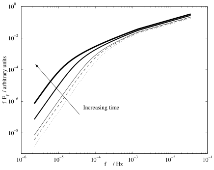
Figure 1: Gravitational wave spectrum arising from constant WD–WD formation rate, at times 2, 5, 10, 100 and 1000 Gyr, increasing in the direction of the arrow shown.

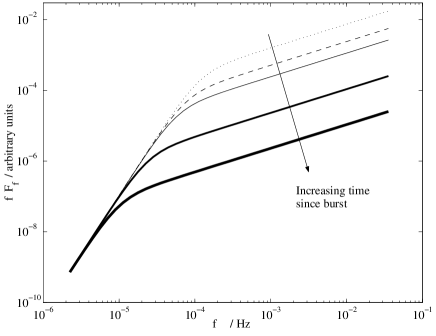
Figure 2: Gravitational wave spectrum arising from a burst of WD–WD formation between 0 and 1 Gyr. Curves plotted are spectra at times 2, 5, 10, 100 and 1000 Gyr, increasing in the direction of the arrow shown.

We therefore expect the cosmological spectrum we calculate later (section 6) to be composed of a superposition of curves of these shapes, modified for chirp mass variations, redshift effects and time delay between progenitor star formation and DD formation. The detailed calculations described in following sections follow in detail the evolution of all sources from ZAMS to merger, and do not rely upon approximate treatments of the kind given above. Simple estimates of the background amplitude are discussed in section 7.

5 Model construction

5.1 The BSE code and population synthesis

The rapid evolution code bse (Hurley, Tout & Pols, 2002) is used throughout this work whenever a binary system is evolved. This code is a fit to detailed models of stellar evolution, and produces an evolutionary time-sequence $x(t_{j})$ of the properties $x$ of any input ZAMS binary system. The code’s time-resolution adapts to the shortest current timescale for change of the system components and orbit, due to e.g. nuclear evolution, angular momentum loss or mass transfer, which are all treated iteratively and have finite duration. In this way, even the most fleeting of evolutionary phases is captured in detail, without requiring excessive time resolution during long phases in which little changes. This is especially useful in the study of gravitational waves, since the majority of the GW emission from a given system occurs over an inspiral timescale much shorter than the nuclear timescales of the binary’s parent ZAMS stars. Some of the most relevant features of the bse code will be described in the following section; see Hurley et al. (2002) for full details.

The output $x(t_{j})$ from the code can be used to construct a stellar population at time $T$ as follows. This method is similar to that used by Hurley et al. (2002) to characterise the Galactic binary population.

We describe the ZAMS binary parameter space in terms of the primary (larger) mass $M_{1}$, secondary mass $M_{2}$ (or mass ratio $q=M_{2}/M_{1}\leq 1$), orbital semi-major axis $a$ and orbital eccentricity $e$. We divide this space into grid boxes, and from each box $k$, we randomly choose a ZAMS system to represent the evolution of all sources in that box.

The number ${\cal P}_{k}$ of sources born into box $k$ per unit binary system realised is determined by probability distributions $A(a)$, $\Xi(e)$ and $\Phi(M_{1},M_{2})=\Phi_{1}(M_{1})f(q)$ in the ZAMS system properties described above (see section 5.3). ${\cal P}_{k}$ is obtained by integrating the product of these distribution functions over the extent of box $k$.

We wish to construct the population of sources present at time $T$. For each output timestep $t_{j}$, the system with properties $x(t_{j})$ can be viewed as a system born between times $(T-t_{j+1})$ and $(T-t_{j})$. If at this point the star formation rate was ${\cal R}={\cal R}(T-t_{j})$ (expressed as a number of binary systems born per unit time), then the number of systems with properties $x(t_{j})$ we expect to see at time $T$ is given by

$${\cal N}_{j,k}(T)=(t_{j+1}-t_{j}){\cal R}(T-t_{j}){\cal P}_{k},$$ (12)

so long as $T>t_{j}$, so that stars were not born before time began. We perform this calculation for all boxes $k$ and all timesteps $j$, so that the total population at time $T$ is given by the combination of all ${\cal N}_{j,k}(T)$.

This method of population synthesis ensures that sources from even unlikely regions of ZAMS parameter space are represented, weighted by their low formation probability. Coupled with the adaptive time-resolution of the bse output, and a sufficiently fine grid spacing, this technique allows the synthesis of a statistically reasonable population in a modest amount of computing time. Alternatively, statistical accuracy can be ensured with a Monte Carlo approach by simply generating a large enough number of stars under the initial distribution functions (see Belczynski et al. 2002).

Our grid extends from 0.08 to 20 M_⊙ in the mass of the primary $M_{1}$, and from 0.08 M_⊙ to $M_{1}$ in the secondary’s mass. The initial separation is gridded from $2(R_{1}+R_{2})$ to $10^{5}(R_{1}+R_{2})$, where $R_{1}$ and $R_{2}$ are the ZAMS radii of the primary and secondary respectively. We find that our background fluxes are statistically accurate to around one per cent if we choose grid spacings of 0.05 in $\ln M$ for each mass and 0.1 in $\ln a$ for the separation. This corresponds to evolving $\sim 7\times 10^{5}$ binaries. For the Galactic tests described in section 5.3 we find that it is sufficient to use a grid spacing twice as large in each dimension.

The bse code has previously been tested against various Galactic populations of binary stars (Hurley, 2000). A set of input parameters and distributions is recommended for use with the code, to best reproduce the observed Galactic binary population as a whole. However, in this work we are keen to quantify the effects of astrophysical uncertainties upon population synthesis calculations of the GW background, and so in the following subsections we construct a set of models which differ in their choice of input parameters but produce specifically a Galactic DD population not in conflict with observations. The current observational uncertainties about DDs admit a range of models. This set of models is then considered representative of the population synthesis uncertainties affecting the GW background.

5.2 The state of observations

The observations of DD stars are currently undergoing a revolution. Full results of this revolution have not yet been published, so the detailed comparison of synthesised populations with observations is still difficult.

Marsh (2000) reported on the 15 then known DDs with measured periods, six of which had measured component mass ratios (Maxted, Marsh & Moran, 2002). Searches for DDs have mainly focussed on low-mass WDs, $M_{\rm{WD}}\la 0.5\rm{~{}M}_{\odot}$ (e.g. Marsh, Dhillon & Duck 1995), since these must have formed through giant stars losing their envelopes in binary systems, before the helium burning that would inevitably occur in a single star. Maxted & Marsh (1999) determined that the fraction of DDs among these DA WDs is between 1.7 and 19 per cent, with 95 per cent confidence. Statistical comparisons with population synthesis models are thus difficult, given the sample size and level of bias, but there are some notable disagreements between observations and theory that are not easily explained in terms of selection effects. The first of these is the lack of observed very low mass He WDs ($M\sim 0.25\rm{~{}M_{\odot}}$). Theory predicts an abundance of such sources. Nelemans et al. (2001b) suggest that this can be explained by a more rapid cooling law for low-mass WDs than is commonly used. The second discrepancy is in the distribution of known DD mass ratios, which is seen to peak near unity (Maxted et al., 2002). Even considering selection effects (Nelemans et al., 2001b), this is difficult to explain in terms of either standard DD formation route, since as described in Section 3, the WD masses are expected to differ significantly.

This prompted Nelemans et al. (2000) to suggest an alternative scenario in which a common envelope phase between a giant and a main sequence star of similar mass does not result in a substantial spiral-in of the orbit, meaning that the second common envelope phase does not occur until the secondary’s radius is larger (relative to that of the primary when it filled its own Roche lobe) than in the standard CEE+CEE picture, so that the second WD formed is more massive, closer to the mass of the first-formed WD. They motivate this choice by parametrizing in terms of an angular momentum, rather than an energy balance (cf. section 3).

The observational sample of DDs is currently being substantially increased by the SPY project (Napiwotzki et al., 2002), a spectroscopic study of $\sim 1500$ apparently single WDs (not restricted to low mass) to search for radial velocity variations indicative of binarity. Napiwotzki et al. (2002) report that of the 558 WDs surveyed so far, 90 (16 per cent) show evidence for a close WD companion. Of these, mass ratio determinations are reported for three DDs (Karl et al., 2002), these three continuing the observed trend of mass ratios near unity.

The results of the SPY project, once analysed fully, will help to constrain DD population synthesis calculations in a greatly improved way. However, given the preliminary and partial nature of the results so far, we can make only rather broad statements about their compatibility with any given synthesised Galactic population. This process is described in the next section.

5.3 Candidate models

Our fiducial population synthesis model (Model A) is similar to the preferred model suggested by Hurley (2000) (also his Model A): we use the initial mass function (IMF) of Kroupa, Tout & Gilmore (1993) (KTG) for $\Phi(M_{1})$, we distribute $M_{2}$ uniformly in the mass ratio $q=M_{2}/M_{1}$, $f(q)=1$, and we start with a flat distribution in $\log a$, choosing our limits as $2(R_{1}+R_{2})<a<10^{5}(R_{1}+R_{2})$, where $R_{1}$ and $R_{2}$ are the ZAMS radii of the primary and secondary respectively. We have tidal effects switched ‘on’, we use $\alpha=3.0$ for the common envelope efficiency parameter, and we assign all stars solar metallicity, $Z=0.02$. For the Galaxy, we adopt the constant star formation rate ${\cal R}$ over the past 10 Gyr which gives a stellar disk mass of $6\times 10^{10}\rm{~{}M_{\odot}}$ today.

We differ from Hurley’s Model A in three main ways: first, we assign an initial binary fraction of 50 per cent (cf. Hurley’s 100 per cent) since this is observed locally to be the case (Duquennoy & Mayor, 1991) and we evolve a set of single stars alongside the binaries, distributed according to the same IMF as the binary primaries. Second, we assign a ZAMS orbital eccentricity $e$ to all systems, according to a thermal distribution $\Xi(e)=2e,0<e<1.0$. Hurley (2000) finds that an $e=0$ model gives a somewhat better fit to observations (though he finds that the numbers of close ($P<10$ d) DD systems produced are not affected); we will also test a model of this type as part of our parameter variation (see below). Lastly, Hurley’s Model A assumed the envelope binding energy parameter $\lambda=0.5$ for all stars, whereas here we allow this parameter to be calculated in the code (values of $\lambda$ are from fits to detailed models of stellar evolution by O. Pols and are an addition to the code described in Hurley et al. 2002; J. Hurley, private communication, 2003), and in addition we include 50 per cent of the envelope’s ionisation energy in its binding energy.

We test our synthesised Galactic populations against observations in a necessarily simple way. The aim is to reject models in clear conflict with the observed population of double degenerate stars, and to admit all others as representative of the uncertainties in DD population synthesis. Since the overall normalisation for the cosmological integral will be entirely separate from that used for the Galaxy, we choose primarily to compare relative populations as opposed to absolute numbers of Galactic sources. An ideal criterion is the fraction among field WDs of close DD binaries, which currently available SPY results place at 16 per cent. Since the sample size is substantially larger than that of Maxted & Marsh (1999), we adopt the SPY data, despite their incompleteness. We assume a negligible false-positive rate for SPY, and approximate the survey as magnitude-limited ($V<15$) for the purposes of comparison. The somewhat approximate Galactic model and star formation history used here are sufficient, given the generosity of our selection criteria and the fact that we compare fractional quantities wherever possible.

We distribute all stars according to a simple double exponential Galactic disk model (scale height 200 pc, scale radius 2.5 kpc), then calculate the fraction of WDs with $V<15$ expected to be members of DD binaries with $P<100$ d. We then require that this calculated fraction be at least 10 per cent, if a given model is to be accepted. We assign a lower limit only, since our calculated binary fractions are likely to be overestimates, for several reasons. First, 100 d is a generous upper limit to the orbital periods detectable with SPY; second, we do not address the issue of the substantial lack of observed low-mass (hence binary-member) WDs found in other population synthesis studies; and finally, the cooling curves used are the simple Mestel curves from Hurley et al. (2002); if we instead use the ‘modified Mestel cooling’ from Hurley & Shara (2003), which better fits the theoretical curves of Hansen (1999), then our calculated binary fraction decreases by a few percent. For our fiducial Model A, with Hurley et al. (2002) cooling, we find that 18 per cent of field WDs will show up as DDs in such a survey, in reasonable agreement with the SPY results.

We also find a local total space density of WDs of $9\times 10^{-3}\rm{~{}pc}^{-3}$, and compare this with observational values, which range from $\sim 4-20\times 10^{-3}\rm{~{}pc}^{-3}$ (Nelemans et al., 2001b, and references therein). We do not attempt to compare to distributions in mass, mass ratio or period in detail: the observed distributions are subject to complex selection effects, and turn out often to be most constraining for WD cooling models (e.g. Nelemans et al., 2001b), whose development is beyond the scope of this paper. We note however that in a volume-limited sense, the mean mass ratio (where $q<1$ by definition) for detached WD–WD pairs is $\left<q\right>=0.62$, not in good agreement with observations, but in common with other studies.

We then go on to consider adjustments to our model, varying the initial distributions and mass transfer prescriptions. In all respects other than those mentioned below, these models are identical to Model A.

In Models B, C and D, we use common envelope efficiency parameters $\alpha$ of 1.0, 2.0 and 4.0 respectively, while Model E uses the angular momentum formalism proposed by Nelemans et al. (2000) for the first phase of spiral in, with their recommended value of $\gamma$, and with $\alpha=4.0$.

In models N, O, P and W, we also perturb the common envelope phase. In Model N, we include all of the envelope’s ionisation energy (a positive quantity corresponding to the energy released when the ionised part of the envelope recombines) in its binding energy, meaning that envelopes will be less strongly bound and hence their removal will require less orbital shrinkage. This effect becomes important for stars on the AGB. Model O, on the other hand, does not include any of the ionisation energy.

Determinations of $\lambda$ from stellar modelling are found to depend on the definition of the core-envelope boundary (Tauris & Dewi, 2001) in giant stars. Because of this uncertainty, we also evolve models W and P in which we fix $\lambda=0.5$, with $\alpha=3$ and $\alpha=4$, respectively.

In Model F, we choose the primary mass from the IMF of Scalo (1986), as in Schneider et al. (2001). Then in Model G we select both $M_{1}$ and $M_{2}$ independently from the KTG IMF, as suggested by Kroupa et al. (1993). We also evolve a Model K, in which initial orbital eccentricities are set to zero.

Models L and M alter the production of DDs via the RLOF+CEE route described in section 3. It has been suggested (Han, Tout & Eggleton, 2000) that Roche lobe overflow may be stable until later in the Hertzsprung gap (HG) than happens using the bse code, so a Model with enhanced HG overflow was added (Model L). Model M has semiconservative overflow during this stage, to emphasise the uncertainties associated with HG mass transfer.

The Galactic DD population was simulated using each model in turn; the results of this exercise are summarised in Table 1. Imposing the criterion given above, we eliminate Models B, G and W based on their under-production of DDs. If we increase the binary fraction to 100 per cent, this tends to under-produce single WDs, leading to an especially high DD fraction and a low overall WD space density. Note that the table also contains a Model H, which is in agreement with observations and is described in the next section.

Thus the models A, C, D, E, F, H, K, L, M, N, O and P progress to the next round, as representative of reasonable astrophysical uncertainties in our population synthesis calculations. Three further models are added later (section 6.4); these vary in their cosmic star formation and metallicity histories, and so cannot be tested against the Galactic DD population.

Table 1: Properties of Galactic DD models; details of models given in section 5.3. % DD is the percentage of field WDs in a magnitude-limited survey that will have a WD companion in an orbit with $P<100$ d. $\rho_{\rm{WD},\odot}$ is the local space density of WDs (single and double). $\left<q\right>_{\rm{vol}}$ is the volume-limited average detached DD mass ratio $q$, where $q\leq 1$ by definition.

Model	% DD	$\rho_{\rm{WD},\odot}$	$\left<q\right>_{\rm{vol}}$	Acceptable?
		$(10^{-3}\rm{pc}^{-3})$
A	18	9	0.62	Yes
B	7	8	0.68	No
C	13	9	0.63	Yes
D	20	9	0.63	Yes
E	24	9	0.75	Yes
F	22	6	0.64	Yes
G	6	6	0.58	No
H	18	9	0.62	Yes
K	17	9	0.63	Yes
L	18	9	0.63	Yes
M	17	9	0.62	Yes
N	17	9	0.63	Yes
O	20	9	0.59	Yes
W	9	8	0.62	No
P	12	8	0.62	Yes

5.4 Interacting DDs and modifications made to BSE code

Some modifications were made to the bse code regarding the treatment of accreting DD systems. In this we mainly follow the recommendations made in the detailed population synthesis work of Nelemans et al. (2001a).

AM CVn stars are mass-transferring compact binaries in which the transfer is driven by gravitational radiation, and in which the accretor is a white dwarf and the donor is a Roche-lobe filling star, which could be another (less massive) white dwarf, or a helium star. For a review, see Nelemans et al. (2001a) and references therein. While not expected to be the dominant source of the Galactic gravitational wave background (Hils 1998; Hils & Bender 2000), some of these systems will be useful as ‘verification’ sources for LISA, with large, predictable gravitational wave amplitudes.

We include in our definition of AM CVns all systems in which a helium star or WD is transferring mass on to a WD, including those systems in which the donor star is a CO or ONe WD.

The WD family

When the donor star is a white dwarf, the orbital separation at initial Roche lobe overflow is around 0.1 R_⊙, which is often sufficiently small that the accretion stream impacts directly on the accretor’s surface, so an accretion disc is not expected to form. This has implications for the orbital evolution of the mass-transferring binary. When an accretion disc is present, tidal torques on the outer edge of the disc return to the orbit the angular momentum carried away from the donor by the accretion stream. In the absence of such a mechanism for restoring the orbital angular momentum, the criterion for stable mass transfer becomes much more stringent, and in most cases an AM CVn star will not form, precluding the existence of the WD family. Here we take the optimistic view (as in model II of Nelemans et al. 2001a) that, even if no disc is present, some tidal mechanism has an equivalent effect and that all WD–WD systems for which the mass ratio is $<0.628$ (Hurley et al., 2002) will commence stable mass transfer upon Roche lobe overflow. We modify the bse code accordingly. This optimism is perhaps warranted, since we do see WD family AM CVn systems, e.g. Israel et al. (2002), which reports on the discovery of a helium-transferring compact binary with orbital period (321 s) too short to involve a (non-degenerate) helium star donor.

The helium star family

In this case, the donor star is a helium star, produced when a star with mass $\ga 2\rm{~{}M}_{\odot}$ loses its envelope on the RGB. Since these stars can live for a rather long time compared with the main sequence lifetimes of their progenitors, there is a significant chance that through GW losses (or sometimes radial evolution) they will commence mass transfer before evolution to the WD stage. Here we shall employ the same condition on the dynamical stability of this mass transfer as Nelemans et al. (2001a): $q=M_{\rm{nHe}}/M_{\rm{wd}}<1.2$ (we use ‘nHe’ to denote (naked) helium star, to avoid confusion with helium-core WDs). Stellar modelling (Savonije, de Kool & van den Heuvel, 1986) indicates that rapid mass transfer forces the helium star out of thermal equilibrium, increasing the thermal timescale beyond a Hubble time. The star cannot ever regain thermal equilibrium, and becomes semi-degenerate (as opposed to fully degenerate) as its mass falls. This results in a negative exponent in the mass-radius relation, so that the orbital separation then increases as the helium star stably loses mass, i.e. an AM CVn system is formed. Note that at the onset of Roche lobe overflow, helium stars are always large enough that an accretion disk can form.

The standard bse code does not incorporate the possibility of these semi-degenerate helium stars, so this was added. Here we adopt the same semi-degenerate mass-radius relation as in Nelemans et al. (2001a) (in solar units):

$$R_{\rm{nHe}}=0.043\,M_{\rm{nHe}}^{-0.062},$$ (13)

and switch between this and the regular non-degenerate relation by selecting the larger of the two radii when the helium star is transferring mass on to a WD companion. In our code, this changeover occurs at $M_{\rm{nHe}}\sim 0.29\rm{~{}M}_{\sun}$. We also modify the mass transfer rate prescription in the code, in order that the transfer responds more quickly to the initial overflow, so that the helium star does not hugely overhang its Roche lobe, and we halt further helium burning, so that the star cannot evolve to the WD stage during transfer, due to its long thermal timescale. We note that this modification is fairly crude, but ought to give a good indication of the relative importance of helium star AM CVn systems as sources of the GW background.

A further issue in the formation of any helium-transferring system is that of edge-lit detonations (ELDs), which are believed to occur after a layer of helium has built up in the surface of an accreting CO WD. The bse code detonates CO WDs in this way after the accretion of 0.15 M_⊙ of helium. We evolve separately a model (Model H) in which this is increased to 0.3 M_⊙, as in Model II of Nelemans et al. (2001a).

6 Cosmological equations

In this section we describe our calculation of the cosmological background. We adopt a standard lambda-cosmology, with $\Omega_{\rm{m}}=0.3$, $\Omega_{\Lambda}=0.7$ and $H_{0}=70$ km s^-1 Mpc^-1. This means that the current age of the universe, $T_{0}=13.5$ Gyr. We assume isotropy throughout; for an analysis of the small anisotropy due to the localisation of binary stars in galaxies which follow the large scale structure of the universe, see Kosenko & Postnov (2000).

6.1 Basic Equations

The specific flux $F_{f_{\rm{r}}}=dF(f_{\rm{r}})/df_{\rm{r}}$ received at frequency $f_{\rm{r}}$ from an object at redshift $z$ with specific luminosity $L_{f_{\rm{e}}}$ is given by (e.g. Peacock, 1999)

$$F_{f_{\rm{r}}}=\frac{L_{f_{\rm{e}}}}{4\pi d_{\rm{L}}(z)^{2}}\left(\frac{df_{\rm{e}}}{df_{\rm{r}}}\right),$$ (14)

where $f_{\rm{e}}=(1+z)f_{\rm{r}}$, $d_{\rm{L}}(z)=(1+z)d_{\rm{M}}(z)$ is the luminosity distance to redshift $z$ and $d_{\rm{M}}$ is the proper motion distance (cf. section 5 of Hogg (2000), which is also $1/(2\pi)$ times the proper (‘comoving’) circumference of the sphere about the source which passes through the earth today).

If the radiation comes from a large number of sources spread over redshift and isotropically distributed on the sky, we can write $dL_{f_{\rm{e}}}(z)=\ell_{f_{\rm{e}}}(z)dV(z)$, where $\ell_{f_{\rm{e}}}(z)$ is the comoving specific luminosity density (say in erg s^-1 Hz^-1 Mpc^-3), $dV(z)=4\pi d_{\rm{M}}^{2}d\chi$ is the comoving volume element and $\chi$ is the comoving distance.

We can then write the specific flux received in gravitational waves today as

$$F_{f_{\rm{\rm{r}}}} = \int^{\infty}_{z=0}\frac{\ell_{f_{\rm{e}}}}{4\pi d_{\rm{L}}^{2}(z)}\left(\frac{df_{\rm{e}}}{df_{\rm{r}}}\right)dV(z)$$ (15)

$$= \int^{T_{0}}_{T=0}\frac{\ell_{f_{\rm{e}}}(T)}{(1+z(T))}\left(\frac{df_{\rm{e}}}{df_{\rm{r}}}\right)c\,dT,$$ (16)

using $d\chi=-(1+z)c\,dT$, where $T$ is cosmic time.

This is the basic equation on which the code is based. The equation is discretised in $f_{\rm{r}}$, $T$ and $\ell$ as described in section 6.2.

6.2 Computational Equations

In the code, we bin the received gravitational waves in frequency. To calculate the flux received in a frequency bin with limits $f_{\rm{r}1}$ and $f_{\rm{r}2}$, we integrate Eq. 16 between these limits:

$$F_{f_{\rm{r}1}\rightarrow f_{\rm{r}2}} = \int_{f_{\rm{r}1}}^{f_{\rm{r}2}}\int^{T_{0}}_{T=0}\frac{\ell_{f_{e}}(T)}{(1+z(T))}\left(\frac{df_{e}}{df_{r}}\right)cdT\,df_{r}$$ (17)

$$= \int^{T_{0}}_{T=0}\int_{(1+z)f_{\rm{r}1}}^{(1+z)f_{\rm{r}2}}\frac{\ell_{f_{e}}(T)}{(1+z(T))}\,df_{e}\,cdT,$$

i.e. we integrate only over those emitted frequencies that will have been redshifted to arrive in this frequency bin today. The bin size was chosen to be $0.1$ in $\log_{10}(f_{\rm{r}})$.

Clearly, to calculate $F$, we need to know the comoving luminosity density $\ell_{f_{e}}$ in gravitational radiation at frequency $f_{\rm{e}}$ as a function of cosmic time.

We first obtain the source population at a given cosmic time $T_{i}$, by simply generalising Eq. 12, so that now

$$N_{k,j}(T_{i})=(t_{j+1}-t_{j}){\cal R}_{c}(T_{i}-t_{j}){\cal P}_{k},$$ (18)

where ${\cal R}_{c}(T)$ is the cosmic star formation rate at time $T$, expressed as a number of binary stars born per unit time per unit volume, and $N_{k,j}(T_{i})$ is the number density of binaries with parameters $k,j$ at cosmic time $T_{i}$, and where we require $T_{i}\geq t_{j}$.

The gravitational wave luminosity density at time $T_{i}$ is then given by

$$\ell_{f_{\rm{e}}}(T_{i})=\sum_{k,j}N_{k,j}(T_{i})L_{k,j}(f_{\rm{e}}),$$ (19)

i.e. we simply sum over the emission at frequency $f_{\rm{e}}$ from all sources $k,j$ present at that time, weighted by their space densities.

Since each binary source $s$ emits radiation at only specific frequencies $f_{n}=n\nu_{s}$ (where $\nu_{s}$ is the orbital frequency of binary $s$) at a given time (Eq. 3), this sum can be expressed as

$$\ell_{f_{\rm{e}}}(T_{i})=\sum_{k,j}N_{k,j}(T_{i})\sum_{n}L_{\rm{circ},k,j}\,g(n,e_{k,j})\delta(f_{\rm{e}}-n\nu_{k,j}).$$ (20)

We then have

$$F_{f_{\rm{r}1}\rightarrow f_{\rm{r}2}}=\sum_{i}\sum_{k,j}\sum_{n_{\rm{min}}}^{n_{\rm{max}}}\frac{N_{k,j}(T_{i})L_{\rm{circ},k,j}\,g(n,e_{k,j})}{(1+z_{i})}\;c\Delta T,$$ (21)

where we have also discretised the integral over cosmic time $T$, as a sum over $i$ intervals $\Delta T$, and where $n$ is an integer, with the limits $n_{\rm{min}}$ and $n_{\rm{max}}$ defined by $f_{\rm{r}1}<\frac{n\nu_{j,k}}{1+z_{i}}<f_{\rm{r}2}$. At a given redshift $z_{i}(T_{i})$, we just sum over those harmonics of those sources that will lead to emission at frequencies $f_{\rm{e}}$, with $f_{\rm{r}1}(1+z_{i})<f_{\rm{e}}<f_{\rm{r}2}(1+z_{i})$, and hence reception in the $f_{\rm{r}1}\rightarrow f_{\rm{r}2}$ frequency bin today.

The integration timestep $\Delta T$ must be sufficiently small that the emitting source population does not change significantly on timescales shorter than this, i.e. we assume a quasi-steady state population during this interval, so that our snapshot of the population at time $T_{i}$ is representative of the whole timestep $\Delta T$. A value of $\Delta T=T_{0}/50$ was used throughout. We checked that timesteps smaller than this did not yield noticeably different results. Individual sources may evolve significantly within this timestep, but the characteristic emission of the population will be unchanged. It should also be noted that the evolutionary timesteps taken for the binary stars are independent of this integration timestep (see section 5.1), so that $\Delta T$ may be made much larger than the timescales of the evolutionary processes of interest, so long as the population is roughly steady-state over $\Delta T$.

Equation 21 is the sum performed by the code written for this paper, for a large number of received frequency bins over the range $10^{-6}<f_{\rm{r}}<10^{0}$ Hz. For practical purposes, the sum over harmonics is truncated when $g(n,e)$ drops below $10^{-3}$, well beyond the peak in the emitted spectrum at $n_{p}=1.63(1-e)^{-3/2}$. For typical $e<0.95$, our numerical cutoff at $g=10^{-3}$ corresponds roughly to including only $n<5n_{p}$. The higher values $n>5n_{p}$ contribute less than 1 per cent of the total gravitational wave luminosity.

6.3 Quantities Used

Some quantities commonly used in gravitational wave astronomy are: $F_{f_{\rm{r}}}(f_{\rm{r}})$, $4\pi$ times the specific intensity; $\Omega_{\rm{gw}}(f_{\rm{r}})$, the fraction of closure density per logarithmic GW frequency interval; and the power spectral density $S_{h}(f_{\rm{r}})$.

The first of these, $F_{f_{\rm{r}}}(f_{\rm{r}})$, can be calculated from

$$F_{f_{\rm{r}}}(\overline{f_{12}})=\frac{F_{f_{\rm{r}1}\rightarrow f_{\rm{r}2}}}{(f_{\rm{r}2}-f_{\rm{r}1})}.$$ (22)

The second, $\Omega_{gw}(f_{\rm{r}})$, is the fraction of closure energy density contained in gravitational waves received in the logarithmic frequency interval around $f_{\rm{r}}$, i.e.

$$\Omega_{\rm{gw}}(f_{\rm{r}})=\frac{1}{\rho_{c}c^{2}}\frac{f_{\rm{r}}F_{f}(f_{\rm{r}})}{c},$$ (23)

where $\rho_{c}$ is the critical mass density of the Universe; $\rho_{c}=(3H_{0}^{2}/8\pi G)\simeq(1.88\times 10^{-29})\,h_{100}^{2}$ g cm^-3, where $H_{0}=100\,h_{100}$ km s^-1 Mpc^-1. In terms of computational quantities,

$$\Omega_{\rm{gw}}(\overline{f_{12}}) = \frac{1}{c^{3}\rho_{c}}\frac{F_{f_{\rm{r}1}\rightarrow f_{\rm{r}2}}}{\Delta(\ln f_{\rm{r}})}$$ (24)

$$\simeq 0.0175\;F_{f_{\rm{r}1}\rightarrow f_{\rm{r}2}}$$

(where $F_{f_{\rm{r}1}\rightarrow f_{\rm{r}2}}$ is in erg s^-1 cm^-2) since $\Delta(\ln f_{\rm{r}})=\ln(10^{0.1})\simeq 0.23$ and $h_{100}=0.7$.

The power spectral density $S_{h}(f_{\rm{r}})$ is given by

$$S_{h}(f_{\rm{r}})=\frac{4G}{\pi c^{3}}\frac{1}{f_{\rm{r}}^{2}}F_{f_{\rm{r}}}(f_{\rm{r}}).$$ (25)

Usually this is plotted as $S_{h}^{1/2}\simeq(5.6\times 10^{-20})\frac{F_{f_{\rm{r}}}^{1/2}}{f_{\rm{r}}}\rm{Hz}^{-1/2}$, where $F_{f_{\rm{r}}}$ is in erg s^-1 cm^-2 Hz^-1, and $f_{\rm{r}}$ is in Hz.

6.4 Cosmic star formation history

As pointed out by Schneider et al. (2001), most determinations of cosmic star formation history are based on the UV emission from massive stars (e.g. Madau et al. 1996; Steidel et al. 1999), and use an assumed single-star IMF (commonly that of Salpeter 1955) to convert observed UV flux into a star formation rate as a function of redshift. This type of rate is inconvenient here for two reasons: first, a non-trivial factor is required for conversion to a binary star formation rate (for an assumed binary fraction), because of the need to correct for the observed flux from companion stars; and second, the total star formation rate is pivoted on the high-mass end of the stellar distribution, while here we are interested in studying the remnants of low- to intermediate-mass stars. This results in a crucial dependence on the choice of stellar IMF.

Schneider et al. (2001) overcome the first problem by assuming the measured shape of the cosmic SFH as a function of time, but normalising its amplitude to the local rate of core-collapse supernovae. This Type Ibc/II SN rate is a more easily calculated quantity for a given (binary or single) IMF than is the UV luminosity density. Since Schneider et al. (2001) are also concerned with neutron stars in their study, this is a reasonable choice. However, the second problem remains when one is concerned with WDs; and in addition, not only does the normalisation pivot on the high mass stars, but it also depends crucially on the ratio of local to peak cosmic SFR. We also note that the minimum mass of star producing a core-collapse supernova explosion is uncertain (e.g. Jeffries, 1997).

For our normalisation, we use instead the observed local stellar mass density $\Omega_{*}$, as derived from the local near-IR luminosity function by Cole et al. (2001). This quantity is most sensitive to stellar masses near the MS turnoff in old populations, $M\sim 0.8-1.0\rm{~{}M}_{\odot}$, and thus is more closely related than the SNIbc/II rate to the DD progenitor population. We convert between their assumed single star IMF and our binary star IMFs by keeping constant the mass in stars in this range. We then use the recycled fraction $R=0.42$, as for the Kennicutt (1983) IMF used in Cole et al. (2001), to convert stellar density today to total mass of stars ever formed, $\Omega_{*,\rm{tot}}$ (the time-integral of the cosmic star formation rate). Doing this, we obtain $\Omega_{*,\rm{tot}}=5.0\times 10^{8}\,\rm{M}_{\odot}\rm{Mpc}^{-3}$ for the KTG IMF, while for the Scalo IMF this figure is $\Omega_{*,\rm{tot}}=4.0\times 10^{8}\,\rm{M}_{\odot}\rm{Mpc}^{-3}$. Due to this rather crude conversion, the uncertainty in these figures will be greater than the 15 per cent quoted by Cole et al. (2001) for $\Omega_{*}$; we estimate the resulting uncertainty to be $\sim$ 30 per cent.

Cole et al. (2001) note that their calculated stellar densities are most consistent with UV-derived star formation rates if the extinction corrections used in these methods are moderate. However, we would like to assess the effects of uncertainty in the shape of the cosmic star formation history. We therefore select both a history with large extinction corrections and one with none, keeping the integral over time fixed to $\Omega_{*,\rm{tot}}$ for each. The corresponding curves are plotted in Fig. 3. We use the extinction-corrected rate, favoured by Steidel et al. (1999), in Model A and all other models except for Model J, which uses the uncorrected rate (but is identical to Model A in all other respects). We also introduce Models Q and R, whose metallicity histories differ from that of Model A: in Model Q, stars born during the first Gyr have metallicity $1/20$ solar, while stars born later have solar composition; in Model R, all stars have metallicity $Z=0.01$, i.e. half-solar.

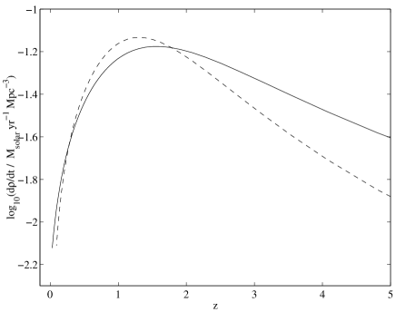
Figure 3: Two possible cosmic star formation histories, plotted as a function of redshift $z$ and parametrized according to the smooth curve fits given in Cole et al. (2001). Dashed line: no extinction correction made, used in Model J. Solid line: extinction corrected with $E(B-V)=0.15$, used in all other Models. The time integral of each rate is fixed using the appropriate $\Omega_{*,\rm{tot}}$ derived from Cole et al. (2001). Curves shown are for the KTG IMF.

7 Basic results

The GW background spectrum received in the frequency range $10^{-6}<f_{\rm{r}}<10^{-1}$ Hz, generated using our fiducial Model A, is plotted in Fig. 4. The total amplitude is broken down into separate contributions from four main evolutionary stages: main sequence–main sequence (MS–MS), WD–MS, WD–WD and WD–helium star (WD–nHe) binaries, and plotted in terms of each of $F_{f_{\rm{r}}}$, $\Omega_{\rm{gw}}$ and $S_{h}^{1/2}$ described in section 6.3. The unitless $\Omega_{\rm{gw}}$ will be our preferred quantity for the remainder of the paper.

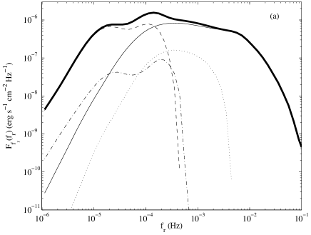
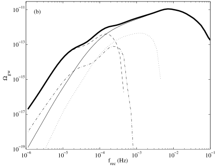
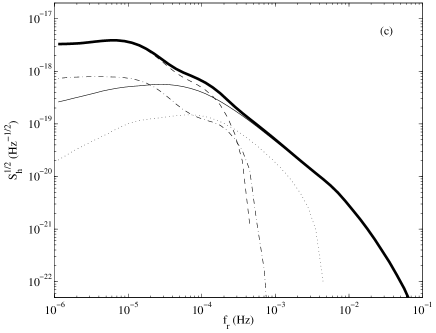
Figure 4: The GW background for our fiducial Model A, in terms of the three quantities described in section 6.3. Solid line: WD–WD pairs; dotted line: nHe–WD pairs; dashed line: MS–MS binaries, and dot-dash line: WD–MS binaries. The total signal (the sum of the four parts) is given by the thick solid line. Only $n=2$ harmonics of the orbital frequency are plotted (see section 7.1.1).

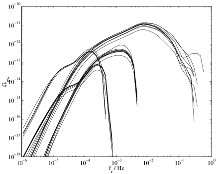
Figure 5: Comparison of spectral shapes for all Models. Curves are the same as in Fig. 4, but all quantities are plotted as solid lines. Only $n=2$ harmonics of the orbital frequency are plotted (see section 7.1.1).

The four component spectra are plotted in Fig. 5 for all of the models evolved, to illustrate that the spectral shapes are largely unaffected by any of the changes made. A summary of important quantities for each model (to be discussed later) is given in Table 2. For reference, we also list a Model A^′, identical in parameters to Model A, to demonstrate the typical level of statistical variation in the results. This is clearly at the 1 per cent level in flux, so that variations larger than this between models can be ascribed to parameter, and not statistical, variations.

Throughout we will focus on the properties of the spectrum around 1 mHz, in the centre of the LISA band and of the spiral-in regime. We will also compare with the spectral properties at 10 mHz, at which frequency lower-mass WD–WD pairs can no longer be present and at which point this extragalactic WD–WD background will be the dominant LISA background source (see Fig. 16).

Table 2: Summary table of results from all models described in the text. $\Omega_{\rm{gw}}$(1 mHz) is in units of $10^{-12}$. R+C refers to the RLOF+CEE route to the DD stage, while C+C refers to the CEE+CEE route (see section 3; note that for Model E, we hold the RLOF+CEE contribution fixed from Model A). The flux-weighted mean chirp mass $\left<{\cal M}\right>$ contributing at $f_{\rm{r}}\sim$ 1 mHz is in units of M_⊙, the next column lists the percentage contribution to $\Omega_{\rm{gw}}$ at 1 mHz from interacting binaries and the last column gives the inspiral remnant density $N_{0}$ today, in units of $10^{6}$ Mpc^-3. Models B and G were rejected for reasons noted in Table 1.

Model	$\Omega_{\rm{gw}}$(1 mHz)			$\left<{\cal M}\right>$	%	$N_{0}$
	Total	R+C	C+C		AM CVn
A	3.57	1.35	2.22	0.45	13	1.17
A′	3.61	1.36	2.26	0.45	14	1.18
C	3.06	0.60	2.47	0.44	16	0.90
D	3.66	1.64	2.02	0.47	13	1.20
E	4.21	1.35	2.86	0.47	10	1.57
F	1.94	0.72	1.22	0.41	13	0.75
H	4.10	1.53	2.58	0.43	25	1.17
J	3.62	1.38	2.24	0.45	13	1.17
K	4.29	2.09	2.20	0.48	13	1.29
L	3.80	1.53	2.27	0.45	12	1.25
M	2.80	0.66	2.14	0.44	15	0.92
N	3.43	1.36	2.07	0.46	13	1.13
O	3.89	1.31	2.57	0.46	13	1.27
P	5.46	1.00	4.46	0.55	16	1.20
Q	3.73	1.43	2.30	0.44	13	1.32
R	3.83	1.48	2.35	0.44	12	1.28

It is clear that the signal in the LISA frequency band ($0.1\la f_{\rm{r}}\la 10$ mHz) is dominated by the WD–WD component, as expected. Neither the MS–MS nor the MS–WD binaries can radiate at frequencies above the bottom of this bandpass, since even the lowest mass MS stars come into contact at frequencies below 1 mHz. WD–nHe pairs can contribute to a somewhat higher frequency due to the smaller radii of helium stars, but still come into Roche lobe contact at $f_{\rm{e}}\sim$ 1 mHz.

The WD–WD component clearly displays the spectral shape predicted in Section 4 ($\Omega_{\rm{gw}}\propto f_{\rm{r}}F_{f_{\rm{r}}}$, plotted in Figs. 1 and 2), with a clear separation between static and spiral-in regimes at around $10^{-4}$ Hz. The slope in the static regime suggests that sources are injected with a spectrum closer to $\dot{N}_{\rm{b}}(\nu)\propto\nu^{-2/3}$ than to $\nu^{-1}$, but agreement to this level is encouraging. The spiral-in slope is slightly steeper than predicted, but this is due to the spectrum seen being the sum of spectra from populations with different chirp masses, as well as different merger and maximum injection frequencies (see Fig. 8), whose individual slopes in the spiral-in regime are closer to the predicted 2/3. Agreement with our simple predictions is therefore good and we feel that we understand well the origins of the spectrum.

7.1 Contributors

The breakdown of contributions to the background received at 1 mHz for our fiducial Model A is given in Table 3. In this section we identify the dominant source types, and those types whose contribution is negligible, then attempt to characterise the emitting population in terms of a mean chirp mass and inspiral remnant density.

Table 3: Percentage contribution to $\Omega_{\rm{gw}}$ at 1 mHz from different DD pairs, for both contribution to total integrated background and contribution to background coming from the local universe, $z=0$. All for fiducial Model A. MS–MS and WD–MS binaries contribute negligibly at this frequency. (‘nHe’ denotes a naked nondegenerate helium star.) All contributions, including the AM CVn values, are given as fractions of the total flux at 1 mHz.

Pairing	% over all time	% locally
He–He	12.4	29.5
He–CO	23.0	25.3
He–ONe	0.6	0.6
CO–CO	42.2	33.2
CO–ONe	8.1	4.4
ONe–ONe	1.0	0.2
(of which AM CVn)	3.6	4.7
nHe–WD	12.7	6.9
(of which AM CVn)	9.7	2.0
Total	100	100
(of which AM CVn)	13.3	6.7

7.1.1 Eccentric harmonics

As described in section 2, systems with eccentric orbits emit gravitational waves at all harmonics $n\nu$ of the orbital frequency, not just the $n=2$ harmonic as for circular orbits.

The only close binaries we expect to be eccentric are unevolved MS–MS binaries in which tidal forces have not yet circularised the orbit. Almost every close evolved (e.g. WD–MS, WD–WD) system will have at some point experienced a Roche lobe-filling phase, which will likely have circularised the system, through tidal circularisation and/or common envelope evolution. Figure 6 shows the contribution from harmonics with $n\geq 3$ to the MS–MS GW spectrum for Model A (which has a thermal initial eccentricity distribution). Clearly the $n\geq 3$ harmonics contribute $\la 10$ per cent of the MS–MS spectrum at frequencies $f_{\rm{r}}\la 0.5\rm{~{}mHz}$, and although they dominate the MS–MS spectrum above this frequency, these signals are buried deep below the other contributors at $f_{\rm{r}}>0.5\rm{~{}mHz}$ (see Fig. 4). Hereafter we safely neglect the $n\neq 2$ contributions to $L_{\rm{gw}}$, in the interests of computing time, though we do not neglect eccentric orbits in computing stellar evolution sequences.

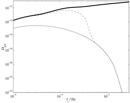
Figure 6: The GW background from harmonics with $n\geq 3$ from MS–MS pairs (thin solid line), plotted along with the total MS–MS pair contribution (dashed line), and the total background from all sources (thick solid line), demonstrating that the harmonic contribution is negligible. All for Model A.

7.1.2 Interacting binaries

Interacting binaries (those in which either a WD or nondegenerate naked helium (nHe) star is transferring mass on to a WD) contribute 13 per cent of the GW background at 1 mHz in Model A. Since at this frequency the majority of nHe star companions fill their Roche lobes, most of the nHe–WD background comes from interacting systems. At 10 mHz, 26 per cent of the GW signal comes from interacting binaries, all of these necessarily WD-donor systems. The GW spectrum due to interacting binaries is compared with the total signal in Fig. 7.

The percentage contribution from interacting systems is fairly constant across models, except for Model H, in which an accreting CO WD is permitted to accumulate 0.3 M_⊙ of helium before detonation, as opposed to the 0.15 M_⊙ in our fiducial model. This increase in survival rate boosts the interacting binary signal at 1 mHz by a factor of two. For the other models, the interacting WD–WD signal is boosted when the WD–WD pairs formed typically have larger mass ratios, so that more systems can commence stable transfer upon Roche contact, e.g. Model C.

The spectral shapes from interacting systems are governed by the mass-radius relation of the Roche lobe-filling star, and so do not share the spectral slopes displayed by the detached binaries. The overall contribution from interacting pairs is sufficiently small, however, that the total spectral shape is little affected by their presence. This is in line with results for the Galaxy found by Hils & Bender (2000) and Nelemans et al. (2001c).

We can predict the spectral shape due to interacting WD–WD binaries using some simple scaling relations (in the notation of section 4): for a Roche lobe-filling WD of mass $M_{\rm{d}}$, we have $M_{\rm{d}}^{-1/3}\propto R_{\rm{d}}=R_{L}\propto aM_{\rm{d}}^{1/3}\propto M_{\rm{d}}^{1/3}f^{-2/3}$, using Kepler’s law (for conservative mass transfer). If we then assume that the mass of the donor WD is much less than that of the accretor, then the system chirp mass ${\cal M}\propto M_{\rm{d}}^{3/5}$, so that $f\propto{\cal M}^{3/5}$ and the system gravitational wave luminosity $L_{\rm{gw}}\propto f^{10/3}{\cal M}^{10/3}\propto f^{16/3}$.

For sources sweeping (backwards) through frequency space, we have $N(f)\propto 1/\dot{f}\propto{\cal M}^{-5/3}f^{-11/3}\propto f^{-14/3}$.

Putting these together, we then have, for the emitted flux in the logarithmic frequency interval around $f$, $\Omega_{\rm{gw}}(f)\propto fF(f)=fL_{\rm{gw}}N(f)\propto f^{5/3}$. From Fig. 7, we measure the spectral slope between 0.4 and 6 mHz to be $\sim$1.7, in good agreement with this calculation. Interacting WD–WD sources are not present below this frequency range because evolution to these frequencies requires more than a Hubble time. Above $\sim 6$ mHz, the spectral shape depends on the fraction of sources of high enough mass to radiate at a given frequency; this number drops rapidly with increasing frequency. Note that, within the 0.4–6 mHz range, since the spectrum $\Omega_{\rm{gw}}\propto f^{5/3}$ for interacting WD–WD binaries rises relative to $\Omega_{\rm{gw}}\propto f^{2/3}$ for inspiralling detached binaries, interacting binaries are more important contributors at high frequencies than at low.

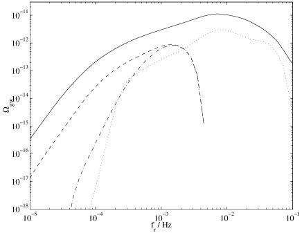
Figure 7: The spectrum due to interacting binaries, for our fiducial Model A. The solid line shows the total WD–WD binary contribution, while the dotted line gives the spectrum from interacting binary WD–WD systems. The dashed line is the total nHe–WD spectrum, of which the dash-dot line gives the interacting nHe–WD contribution.

7.1.3 WD types, chirp mass and merger rates

The dominant component of the background at frequencies 0.1–10 mHz comes from the inspiral of WD–WD systems. From Table 3, we see that approximately half of this background comes from CO–CO pairs, descended primarily from higher mass progenitors than the majority of He–He systems. The dominance of these systems is a result of both the shorter time delay between star formation and DD birth for more massive MS stars, and the larger chirp masses for CO–CO systems, since the flux in the inspiral part of the spectrum scales as $\Omega_{\rm{gw}}\propto f_{\rm{r}}^{2/3}{\cal M}^{5/3}$ (see section 4). These two factors outweigh the fact that, from the IMF, many more potential progenitors of He WDs are born than those which always produce CO or ONe WDs after envelope loss.

Figure 9 shows however that, as more low-mass MS stars evolve to the DD stage, the relative contribution to the GW luminosity density from pairs involving He WDs is rising, and will eventually dominate. The percentage contribution to the local ($z=0$) WD–WD GW emission at 1 mHz from pairs including at least one He WD is 55 per cent, whereas their contribution to the integrated cosmological background received today is only 36 per cent.

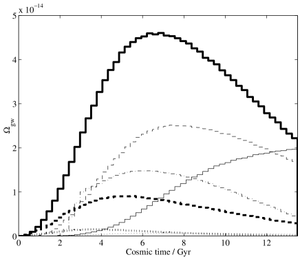
Figure 9: The contribution to $\Omega_{\rm{gw}}$(1 mHz) received today as emitted from each shell of cosmic time, $\Delta T=T_{0}/50$, from each source type, for Model A. Linestyles are as in Fig. 8, with the addition of the thin dash-dot line for nHe–WD pairs.

A useful way to look at this is through the chirp mass distribution. Shown in Fig. 10 is the contribution to $\Omega_{\rm{gw}}$ at 1 mHz as a function of system chirp mass (defined in section 4) for Model A, giving a flux-weighted mean chirp mass of $0.45\rm{~{}M}_{\odot}$. As increasingly lower mass systems evolve off the main sequence and become close DD pairs, this mean chirp mass is decreasing with time, as shown in Fig. 12. The chirp mass distribution depends on GW frequency (Fig. 11), most notably shifting towards higher masses at frequencies above which lower-mass WD–WD pairs will have merged. The mean chirp mass is somewhat higher below the critical spiral-in frequency, since for $f_{\rm{e}}<2\nu_{\rm{crit}}$, we have $\Omega_{\rm{gw}}\propto{\cal M}^{10/3}$, and above $2\nu_{\rm{crit}}$, $\Omega_{\rm{gw}}\propto{\cal M}^{5/3}$ (see section 4).

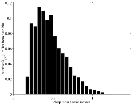
Figure 10: Relative contribution to $\Omega_{\rm{gw}}$ at 1 mHz as a function of chirp mass, for Model A, giving a mean flux-weighted chirp mass $\left<{\cal M}\right>=0.45\rm{~{}M}_{\odot}$.

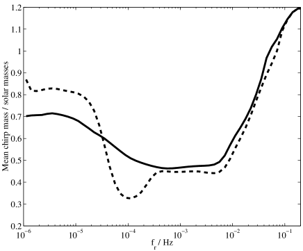
Figure 11: Flux-weighted chirp mass contributing to the GW background received, as a function of frequency, for Model A. Solid line: detached WD–WD pairs only, dashed line: all source types. The dip seen in this curve around 0.1 mHz is due to low-mass main sequence stars.

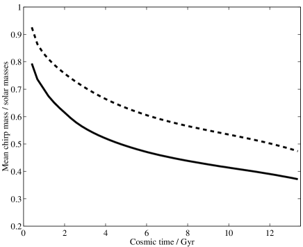
Figure 12: The flux-weighted mean chirp mass contributing to emission received today at 1–3 mHz (solid line) and 3–10 mHz (dashed line), from each shell of cosmic time. All for Model A.

Phinney (2002) derived a simple expression for the GW background in terms of the chirp mass ${\cal M}$, assumed constant across all sources, and the current space density $N_{0}$ of remnant spiralled-in sources (with a weak dependence on cosmology and star formation history). We can assess the usefulness of this formula as a predictor of the background flux by using the results of our population synthesis calculations to see whether the computed fluxes can indeed be described by these two parameters only.

To calculate the remnant density $N_{0}$, we first calculate the source spiral-in rate as a function of cosmic time. The rate of occurrence of Roche lobe contact between WD–WD pairs (we shall call this the spiral-in rate) is different from the rate of WD–WD mergers, since for some subset of systems (those with mass ratios $q<0.628$) stable mass transfer will commence upon overflow, and an AM CVn system will form. We keep track of both of these rates here.

For $f$ greater than both $2\nu_{\rm{max}}$ and $2\nu_{\rm{crit}}$, i.e. in the part of the spiral-in regime above which sources are born (see section 4), then for a quasi-constant spiral-in rate $\dot{N}$ over the timestep $T_{0}/50$, the continuity equation (Eq. 6) simplifies to

$$\dot{N}=\sum_{i}\dot{\nu}N_{i},$$ (26)

summed over all sources $i$ at any given frequency satisfying the above requirement. For each source, $\dot{\nu}$ is given by Eq. 7. We perform this sum at each step in cosmic time, using systems with orbital frequencies in the range $0.8<\nu<1.6$ mHz, which is above the maximum injection frequency for the majority of sources, and below those frequencies at which the lowest mass WDs are coming into contact. We note that the inspiral time from $\nu\sim$ 0.5 mHz is less than $T_{0}/50=0.27$ Gyr for all ${\cal M}\ga 0.05\rm{~{}M}_{\odot}$, so that at each timestep we are accurately representing the spiral-in rate at that time. The only exceptions are very low chirp mass systems, which we neglect here anyway, since these will be interacting binaries, which are spiralling out. We also neglect all nHe–WD pairs, since the evolution of these systems is not governed exclusively by gravitational radiation, but also via radial evolution of the nHe star, and also because Roche lobe contact occurs for these systems within our frequency range.

The spiral-in and merger rates obtained from Model A are plotted in Fig. 13. The present-day remnant density $N_{0}$ needed for the formula of Phinney (2002) is the time integral of the spiral-in rate, since this gives the total number of sources that have contributed to the background. From our calculated rate, we obtain $N_{0}=1.17\times 10^{6}\rm{~{}Mpc}^{-3}$.

Phinney (2002) deals only with the GW emission from non-interacting WD–WD systems, and so we should compare its predictions with only the non-interacting component of our computed signals, in addition to using a characteristic chirp mass ${\cal M}^{\prime}$ for just those systems. For Model A, our flux-weighted mean chirp mass for detached WD–WD pairs is $\left<{\cal M}^{\prime}\right>=0.47\rm{~{}M}_{\odot}$ at 1 mHz. Eq. 16 of Phinney (2002), converting to $h_{100}=0.7$, and omitting the $\left<(1+z)^{-1/3}\right>$ scaling factor in the interests of simplicity, becomes

$$\Omega_{\rm{gw}}=1.1\times 10^{-17}\left(\frac{{\cal M}^{\prime}}{\rm{M}_{\odot}}\right)^{5/3}\left(\frac{N_{0}}{\rm{Mpc}^{-3}}\right)\left(\frac{f_{r}}{1\rm{~{}mHz}}\right)^{2/3}.$$ (27)

Using $\left<{\cal M}^{\prime}\right>$ and $N_{0}$ for Model A in the above, we find $\Omega_{\rm{gw}}\rm{(1~{}mHz)}=3.7\times 10^{-12}$. We compare this with the computed value for detached WD–WD pairs, $\Omega_{\rm{gw}}(\rm{1~{}mHz})=3.0\times 10^{-12}$, and note that these agree to within 25 per cent. If we perform this same calculation for the other Models, we find that Eq. 27 overestimates the computed background by a similar fraction.

The variation between models is thus well fitted by the formula. The relative fluxes are reproduced by Eq. 27 to within 5 per cent for all Models except D and E, whose fluxes relative to Model A are overestimated by 7 and 16 per cent respectively. The dominant scaling is due to variations in $N_{0}$, since in most cases $\left<{\cal M}^{\prime}\right>$ varies little between Models. For the cases in which $\left<{\cal M}^{\prime}\right>$ does significantly change (D, E, F, K and P), the omission of the chirp mass scaling in Eq. 27 can improve (D, E) or worsen (F, K, P) the agreement with the results of our detailed calculations. This is perhaps as expected, since our flux-weighted chirp mass is in fact not the same average as that required in the generalisation of Phinney (2002) to accommodate a range of chirp masses. Such a value would also incorporate the redshift-scaling omitted in the above. We note, however, that neither $N_{0}$ nor either definition of ${\cal M}^{\prime}$ is a directly observable quantity, requiring as they do integrations over cosmic time, and so are not easily determined from observations.

The computed spectral shape is not precisely $\Omega_{\rm{gw}}\propto f_{\rm{r}}^{2/3}$ (see Fig. 4), so we do not expect an exact reproduction of the spectrum using this formula. However, we conclude that with a knowledge of $N_{0}$ and ${\cal M}^{\prime}$, we can quickly predict the detached WD–WD background amplitude and to some extent its variation if these values change. We note however that a full population synthesis calculation enables the inclusion of interacting systems, as well as the extraction of detailed spectral shapes and source property distributions, which are not available in a quick ‘manual’ calculation.

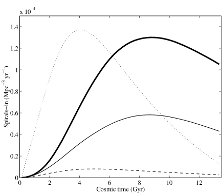
Figure 13: The rate of WD–WD spiral-in as a function of cosmic time. The thick solid line gives the total spiral-in rate, while the thin solid line shows the merger rate, that is the inspiralling sources that will merge, and not commence stable mass transfer (i.e. become AM CVn binaries) upon Roche lobe overflow. The thin dashed line gives the rate of merger of WD–WD pairs with combined mass $>1.4$ M_⊙. For reference, the cosmic star formation rate, multiplied by $1/(1000\rm{M}_{\odot})$, is plotted as the thin dotted line. All for Model A.

7.2 Progenitors

Here we outline the relative contributions from the two main pathways to the DD stage, and we assess the impact upon each of these routes of varying the population synthesis model.

Figure 14 shows the contribution to $\Omega_{\rm{gw}}$ at 1 mHz as a function of the initial mass of the primary, for Model A. The descendants of primaries with ZAMS masses in the range 2–4 M_⊙ contribute 50 per cent of the signal, the flux-weighted mean progenitor primary mass being 3.7 M_⊙. Most of the sources in this range are the progenitors of CO WDs, since for $M\ga 2\rm{~{}M}_{\odot}$, a CO WD will be produced via a helium star upon envelope loss on the RGB, and a CO WD will be produced directly if the envelope is lost on the AGB. At 10 mHz, the mean progenitor mass rises to 4.7 M_⊙, since the (necessarily more massive) WD–WD pairs contributing there are descended from only the more massive ZAMS systems. The equivalent secondary mass distribution is not plotted here, but is always peaked towards initial mass ratios of unity.

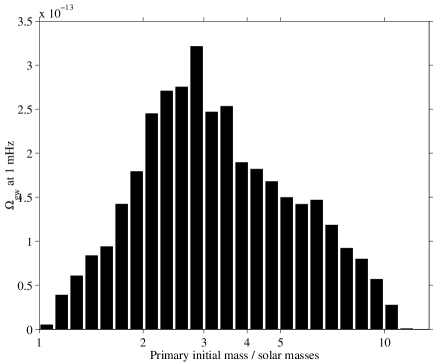
Figure 14: Contribution to $\Omega_{\rm{gw}}$(1 mHz) received, as a function of ZAMS mass of the primary, for our fiducial Model A.

Of perhaps more interest is the distribution in initial orbital semimajor axis (Fig. 15, for Model A), which has a clear bimodal form, the peak at $a\sim 5a_{\rm{min}}$ corresponding to DDs which formed via RLOF+CEE, and the peak at $a\sim 50a_{\rm{min}}$ corresponding to the CEE+CEE route. We can therefore approximately determine the relative contributions from these two routes by dividing this distribution between the two peaks (at $a\sim 10a_{\rm{min}}$ for most models); the result of this division for each model is shown in Table 2. We note that the location of the CEE+CEE peak at $a\sim 50a_{\rm{min}}$ and the typical masses of the dominant progenitor stars mean that for this route, the dominant pathway involves primary overflow on the AGB, followed by secondary overflow on its RGB.

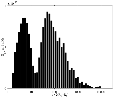
Figure 15: Contribution to $\Omega_{\rm{gw}}$(1 mHz) received, as a function of initial progenitor semimajor axis, expressed as a ratio of the initial semimajor axis to the minimum separation permitted in the code. For Model A.

For Model A, $\Omega_{\rm{gw}}\rm(1~{}mHz)=1.4\times 10^{-12}$ ($\sim 38$ per cent of the total) comes from sources that evolved via the RLOF+CEE pathway. Since the WD–WD pairs from this route are generally more massive than CEE+CEE pairs, the percentage contribution at 10 mHz from this route rises to 44 per cent.

In general, we shall find that it is the RLOF+CEE contribution that is affected more by varying the population synthesis model. Although it can be affected significantly by varying the form of the common envelope prescription (Models E and P), the CEE+CEE signal is quite robust to changes in the common envelope efficiency, since if systems originating at one separation happen to coalesce in a common envelope phase, using a given model, there exists a shell of sources at greater $a$ to take their place as the closest WD–WD systems at birth, out to a maximum of $a\sim 10^{3}a_{\rm{min}}$ at which Roche lobe overflow no longer occurs on the RGB or AGB. Webbink & Han (1998) describe this effect in terms of shifting the ‘window’ in initial parameter space from which the closest DD systems are descended. The weak dependence of results upon the common envelope efficiency parameter is also seen in population synthesis calculations for other types of binary, e.g. Kalogera & Webbink (1998) for LMXBs.

Returning to the DD case, the RLOF+CEE pathway has no similar resource, occurring only in the rather narrow range of initial separation in which RLOF commences in the Hertzsprung gap. If we destroy more of these sources in the ensuing CEE phase, we lose more of the contributions from the RLOF+CEE route.

Decreasing $\alpha$ (Model C) has this kind of deleterious effect upon the RLOF+CEE pathway, but slightly increases the signal from CEE+CEE sources, since the systems which survive to the close DD stage were on average more widely spaced than for $\alpha=3.0$, so that the giant stars were physically larger, i.e. more evolved, on average upon Roche lobe overflow, so gave rise to more massive WDs (also with more widely differing masses). This corresponds to moving the second peak in Fig. 15 to higher $a$. The lower mean chirp mass is largely attributable to the increased number of low-chirp mass interacting binaries present at this frequency, since the typical WD–WD mass ratio is larger, as described in section 7.1.2. Increasing the efficiency parameter (Model D) has the opposite effect upon each route. If on the other hand we use the common envelope formalism of Nelemans et al. (2000) (Model E), it becomes less simple to disentangle the two routes, since now they overlap somewhat in initial $a-$space, but since we know that this modification ought not to affect the RLOF+CEE contribution, we hold this fixed from Model A. The new CEE+CEE value turns out to be significantly enhanced, since a wider range of initial separations has been opened up to double common envelope survival. The nearer (by design) equality of WD pair masses leads to a decrease in the number of WD–WD AM CVn systems produced, and hence a smaller contribution from interacting systems than for Model A.

The envelope ionisation energy becomes a significant part of the energy balance in AGB stars, and so its inclusion is important in common envelope phases that commence at large orbital separations. Increasing the fraction of this energy included in the envelope binding energy (Model N) therefore decreases the number of wide binaries able to shrink enough to form close WD–WD pairs. Omitting it entirely (Model O), thus increasing the envelope binding energy, has the opposite effect.

Model P shows the greatest departure from Model A in terms of GW flux and mean chirp mass. The progenitor mass distribution for Model P is peaked towards higher mass (6 – 8 M_⊙) stars than for other Models. These differences can be traced to the outcome of common envelope phases on the Hertzsprung Gap (HG). The bse fitting formula returns values of $\lambda$ substantially smaller than 0.5 for most HG stars, corresponding to a high degree of central concentration. Therefore using $\lambda=0.5$ in Model P results in much less shrinkage in these situations.

High mass stars expand in radius by a large factor in their HGs, so that the final Roche contact (for both pathways) is often a common envelope phase involving a HG star. The survival rate from this CE phase is boosted by the fixed lambda as described above. The resulting GW flux is therefore also greatly boosted for these higher mass stars, whose descendent WDs are sufficiently massive that relatively few are required to dominate the background GW flux. Given however that small values of lambda are robust for HG stars (they are also seen in the calculations of Dewi & Tauris 2000), we choose not to consider this prescription as a reasonable uncertainty on the background.

The lower chirp mass $\left<{\cal M}\right>$ seen for Model H is due to the inclusion of an increased number of interacting sources at 1 mHz, compared with Model A; the value $\left<{\cal M}^{\prime}\right>$ appropriate for just detached WD–WD pairs for this model (used in the previous section) is the same as for Model A.

Starting all systems with circular orbits (Model K) boosts the RLOF+CEE pathway, because fewer systems given initially tight orbits are lost due to immediate collision at periastron. Since systems descended from the RLOF+CEE route are generally higher-mass, the mean chirp mass for Model K is higher than for Model A. CEE+CEE route systems are little affected; the high-$a$ peak in Fig. 15 is simply narrowed in $a$-space, since orbital separations are no longer altered by tidal circularisation before Roche contact.

Aside from orbital circularisation, the main role of tides in the evolution to the DD stage is in orbital shrinkage before Roche contact, due to spin-up of the giant star. Neglecting tidal effects is thus similar to increasing the common envelope efficiency parameter, i.e. the progenitors of close DDs from the CEE+CEE route have smaller initial orbital separations, and the DDs produced have smaller chirp masses on average. If on the other hand tidal effects were much stronger than in the bse code, then we would expect little impact upon this route, since giant-star corotation is already typically achieved before Roche lobe overflow with the tides in bse.

The CEE+CEE route is as expected largely unaffected when we perturb dynamically stable mass transfer on the Hertzsprung gap. Much as one might expect, the RLOF+CEE route is enhanced when one enhances the transfer on the Hertzsprung gap (Model L), so that more mass is transferred to the companion, and more systems avoid a common envelope phase during the first phase of mass transfer (which tends to lead to merger). The orbit is also widened to a greater extent during transfer, meaning that more systems will survive the common envelope phase when the secondary evolves. Making the transfer semi-conservative (Model M) has an opposing effect; the orbit is widened less during stable overflow, meaning that more systems are destroyed in the ensuing common envelope phase.

The steeper Scalo IMF (Model F), normalised to the local space density of low-mass stars, produces fewer intermediate (and high) mass stars than the KTG IMF, and so fewer of the dominant progenitors in Fig. 14 are produced. More of the compact binaries are then descended from lower-mass progenitors than for Model A, giving rise to their lower mean chirp mass. If we had instead normalised to the local core-collapse supernova rate, as in Schneider et al. (2001), we would instead have ended up with a correspondingly higher background from Model F.

Altering the shape of the cosmic star formation history (Model J) has little impact upon the background, since most of the sources contributing have MS evolution times of less than a few Gyr (see Fig. 14). This is a strong argument in favour of using an integral constraint (such as IR luminosity density), and not a present-day constraint (such as local core-collapse supernova rate), since normalising according to the supernova rate introduces a strong dependence on the shape of the cosmic star formation history curve, through the difference in amplitude between the local rate and the rate at the peak of star formation, which can easily skew the overall normalisation.

Finally, Models Q and R lead to larger gravitational wave backgrounds than Model A, mainly because lower metallicity stars tend to leave the main sequence earlier, and thus a greater fraction of the stellar mass in the universe today is present in the form of remnants. The difference in received flux is, however, slight, on the order of 10 per cent. We conclude that keeping detailed track of abundance variations is not essential to calculation at the present level of accuracy.

8 Outlook

Table 4: Summary of the properties of the optimistic and pessimistic models, along with the fiducial Model A

Model	% DD	$\left<q\right>$	$\Omega_{\rm{gw}}\rm{(1~{}mHz)}$	$\left<{\cal M}\right>$	$N_{0}$
Optimistic	26	0.75	5.99	0.46	1.85
A	18	0.62	3.57	0.45	1.17
Pessimistic	14	0.66	0.95	0.40	0.32

Based on the above indications of which effects boost the GW background and which reduces it, we construct two models in an attempt to put upper and lower limits on the background we predict. Our use of the terms ‘optimistic’ and ‘pessimistic’ assumes that this background constitutes signal for the reader; if it constitutes a noise, the nomenclature should be reversed.

Optimistic model: This has the properties of Model A, except for: the Nelemans et al. (2000) common envelope formalism, initially circular orbits, enhanced mass transfer on the HG, edge lit detonations only after accretion of 0.3 M_⊙ and no ionisation energy in envelope binding energies used for common envelope phases. Note that some of these individually boosting effects do not make a double-boost in combination; for example the no spiral-in common envelope prescription tends to lead to DD mass ratios closer to unity, which means that fewer systems undergo stable mass transfer upon contact, and so the enhancement brought by the higher ELD limit is less effective in increasing the amplitude of the background. We also include the estimated error on our overall normalisation (see section 6.4), by using a cosmic star formation rate everywhere 30 per cent higher than our fiducial one.

Pessimistic model: The pessimistic model contains the elements found in the previous section to decrease the amplitude of the GW background. The properties of this model are thus the same as Model A, except for: $\alpha=2.0$, Roche lobe overflow is semiconservative on the HG, the Scalo initial mass function is used and 100 per cent of the ionisation energy is included in the envelope binding energies used in common envelope phases. In addition, we use a star formation rate everywhere 30 per cent lower than our fiducial one, in our cosmological integral.

These prescriptions were used to create Galactic DD populations, which were found to compare reasonably with observations. Then the cosmological integrals were carried out for each. The results of this are summarised in Table 4, and the optimistic, fiducial and pessimistic total background spectra are plotted in Fig. 16 along with the LISA sensitivity curve, and the Galactic WD–WD background taken from Nelemans et al. (2001c). We plot both the ‘unresolved’ (‘average’) background curve from their paper, which is for DD pairs only, with the resolved sources removed, and an extrapolated ‘total’ background. In this we have added back in the resolved close binaries and made an approximation to the MS–MS contribution at lower frequencies, in an attempt to represent the Galactic signal over the full frequency range plotted.

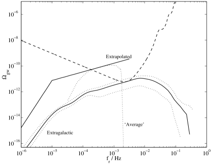
Figure 16: Optimistic (upper dotted), fiducial (Model A, lower solid line) and pessimistic (lower dotted) extragalactic backgrounds plotted against the LISA (dashed) single-arm Michelson combination sensitivity curve (see http://www.srl.caltech.edu/$\sim$shane/sensitivity/). The ‘unresolved’ Galactic close WD–WD spectrum from Nelemans et al. (2001c) is plotted (with signals from binaries resolved by LISA removed), as well as an extrapolated total, in which resolved binaries are restored, as well as an approximation to the Galactic MS–MS signal at low frequencies.

Plotted in Fig. 17(a) is the number of systems per 1/(3 yr) frequency resolution element contributing to the GW background as received today. We see from this that at frequencies $f_{\rm{r}}\la 50$ mHz, there will be too many individual WD–WD sources contributing in each resolution element for this background to be completely resolved and subtracted source by source by missions with plausible lifetimes. However, from Fig. 17(b), we see that much of the flux comes from relatively nearby sources, and the WD–WD numbers drop rapidly above 50 mHz (leaving the lower background from rare neutron stars and black holes, not considered in this paper). Thus it may be possible for future missions more sensitive than LISA to subtract this background at high frequencies.

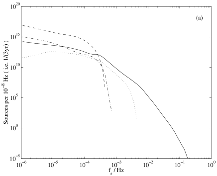
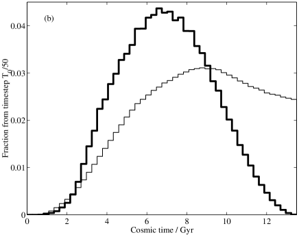
Figure 17: (a) The number of systems per $10^{-8}$ Hz contributing to the cosmological GW background as received today. Linestyles denote the evolutionary classes as in Fig. 4. (b) Thin line: the fractional contribution at 10 mHz to the GW background as a function of cosmic time (from shells of width $T_{0}/50$). Thick line: the same, but in terms of the number of sources contributing to the flux received from each cosmological time-shell.

9 Comparison with previous work

Hils et al. (1990) and Kosenko & Postnov (1998) each made an order of magnitude estimate of the ratio of the extragalactic to Galactic GW flux from DDs. In order to facilitate comparison, and to compare like with like as far as possible, we divide our calculated extragalactic flux at 1 mHz by the most recently calculated value (Nelemans et al., 2001c) for the Galactic flux at the same frequency (which is a factor $\sim 3$ smaller than that found by Webbink & Han 1998). The correct curve from Fig. 16 to use for this comparison is our ‘extrapolated’ curve. We find $\Omega_{\rm{extragal}}/\Omega_{\rm{gal}}=$ 2.0 per cent at 1 mHz for Model A, with a range of 0.5 – 3.4 per cent between optimistic and pessimistic Models.

Hils et al. (1990) predicted a factor $\sim$ 1.6 per cent (for an Einstein-de Sitter universe with no cosmological evolution of galactic GW luminosity). This estimate is in good agreement with our value.

Kosenko & Postnov (1998), on the other hand, predicted that, for a cosmology of the type used in this paper, the extragalactic background should be of order 10 per cent of the Galactic one, when one takes into account the evolution of star formation rate with redshift. This result is in clear disagreement with our findings, but this can be explained by noting that their ratio is artificially raised by a number of factors: first, the fiducial scalings of $\Omega_{\rm{b}}$, $\left<r\right>$ and $h_{100}$ in their eq. 13 are higher than their true values, boosting the extragalactic signal. Second, the same star formation rate as a function of redshift was used for different cosmologies, which leads to an artificial boost to the lambda-cosmology extragalactic flux (see e.g. Somerville, Primack & Faber, 2001). Lastly, the cosmic star formation rate adopted was not normalised to any integral constraint, but merely to the current star formation rate. All of these factors lead to their calculation yielding a misleadingly high extragalactic contribution to the GW background.

Schneider et al. (2001) made a more direct calculation of the background. At 1 mHz, their derived background level (for $h_{100}=0.7$) is $\Omega_{\rm{gw}}=1.2\times 10^{-11}$, with no quoted uncertainty on this value. This lies a factor two outside of our predicted range for the background. The discrepancy can be understood mainly in terms of their different method of normalisation: they normalised to the local core collapse supernova rate, and used the steep Scalo IMF, meaning that more low- and intermediate-mass stars were born in their simulations than measured by Cole et al. (2001). As explained in Section 6.4, we believe that normalising to an integral constraint on the birth of low-mass stars is a more robust method. Schneider et al. (2001) also used a binary fraction of 100 per cent, cf. our 50 per cent.

The shape of the spectrum in Schneider et al. (2001), however, we cannot explain. The spiral-in part of the spectrum ($f_{\rm{r}}\ga 10^{-4}$ Hz) has the form expected from Section 4, but the static regime instead displays a prominent ‘bump’ at frequencies ($f_{\rm{r}}\sim 3\times 10^{-5}$ Hz) just below the transition to the spiral-in regime, the amplitude of which decays rapidly towards lower frequencies. No such feature is seen in our calculated spectra. This type of feature is difficult to explain in terms of the arguments in Section 4, unless the vast majority of WD–WD pairs are born precisely into this ‘bump’, which seems unlikely, since the same feature is seen for all types of compact object pair (e.g. NS–NS, NS–BH), despite their very different formation routes.

10 Conclusions

We predict that the background of gravitational waves from extragalactic binary stars is

1. Dominated by double main sequence binaries for $f_{\rm{r}}<10^{-4}$ Hz.

2. Dominated by double white dwarf binaries for $10^{-4}<f_{\rm{r}}<10^{-1}$Hz.

Concentrating on the spectrum around $1$ mHz:

1. The fraction of critical density in gravitational waves received in the logarithmic frequency interval around 1 mHz lies in the range $1\times 10^{-12}<\Omega_{\rm{gw}}<6\times 10^{-12}$, with the most likely value in the range $3-4\times 10^{-12}$.

2. The flux-weighted mean chirp mass of the contributing binaries is $\langle{\cal M}\rangle=0.45\rm{~{}M}_{\odot}$.

3. Half of the background comes from binaries whose more massive (primary) star had a mass in the range 2–4 $\rm{M}_{\odot}$ (and $\sim$70 per cent from primaries originally less massive than 4 M_⊙). The estimate of the background is thus more robust to uncertainties in the IMF and mass cuts if normalised to the present density of starlight than if normalised to core-collapse supernova rates.

4. $\sim 60$ per cent of the GW signal is from binaries with initial semi-major axes in the range of 30–1000 stellar diameters, in which the Roche contact of both primary and secondary stars led to unstable transfer and a common envelope. The background level produced by these systems is quite stable against uncertainties in the efficiency of the common envelope phase, though the signal can be changed somewhat through use of a non-standard common envelope prescription.

5. $\sim 40$ per cent of the GW flux comes from systems descended from binaries with initial semi-major axes of about 5 stellar diameters, in which the first Roche contact occurred in the Hertzsprung gap, with stable overflow, but the second Roche contact led to unstable transfer and a common envelope. The background level produced by these systems is sensitive to uncertainties in common envelope and mass transfer physics.

6. interacting systems (AM CVn binaries) contribute only about 10 per cent of the energy density in gravitational waves.

The above holds true for $0.5\la f_{\rm{r}}(\rm{mHz})\la 5$. Above this range, as the lower-mass WD–WD pairs reach contact and drop out of the spectrum due to mergers, the properties change (values at 10 mHz in the parentheses which follow): the contribution from interacting binaries increases (26 per cent), the RLOF+CEE route contribution (44 per cent) and the mean primary progenitor mass increase (4.7 M_⊙) and the mean chirp mass is higher (0.56 M_⊙).

We find that at all frequencies, our derived spectral shape can be understood in terms of simple arguments, and that this shape is essentially independent of the population synthesis model used.

References

- Apreda et al. (2002) Apreda R., Maggiore M., Nicolis A., Riotto, A. 2002, Nucl. Phys. B 631, 342
- Belczynski et al. (2002) Belczynski K. Kalogera V., Bulik T. 2002, ApJ 572, 407
- Cole et al. (2001) Cole S. et al. (2dFGRS Team), 2001, MNRAS, 326, 255
- Cornish & Larson (2002) Cornish N., Larson S. L. 2002, gr-qc/0206017
- Dewi & Tauris (2000) Dewi J. D. M., Tauris T. M. 2000, A&A, 360, 1043
- Duquennoy & Mayor (1991) Duquennoy A., Mayor M., 1991, A&A, 248, 485
- Evans et al. (1987) Evans C. R., Iben I, Smarr L. 1987 ApJ 323, 129
- Finn & Thorne (2000) Finn L. S., Thorne K. S. 2000, Phys. Rev. D 62, 124021
- Giampieri & Polnarev (1997) Giampieri G., Polnarev A. G. 1997, MNRAS 291, 149
- Han et al. (2000) Han Z., Tout C. A., Eggleton P. P., 2000, MNRAS, 319, 215
- Hansen (1999) Hansen B. M. S., 1999, ApJ, 520, 680
- Hils (1998) Hils D., 1998, in Folkner W. M., ed, AIP Conf. Proc. Vol. 456, Second International LISA Symposium on the Detection and Observation of Gravitational Waves in Space, p68
- Hils & Bender (1995) Hils D., Bender P. L., 1995, ApJ, 445, L7
- Hils & Bender (2000) Hils D., Bender P. L., 2000, ApJ, 537, 334
- Hils et al. (1990) Hils D., Bender P. L., Webbink R. F., 1990, ApJ, 360, 75 (errata ApJ, 369, 271)
- Hogan (2000) Hogan C. J., 2000, Phys Rev D, 62, 121302
- Hogan & Bender (2001) Hogan C. J., Bender P.L., 2001 Phys Rev D, 64, 062002
- Hogg (2000) Hogg D. W., 2000, astro-ph/9905116
- Hughes (2001) Hughes S. A., 2001, Class. Quant. Grav. 18, 4067
- Hurley (2000) Hurley J. R., 2000, PhD Thesis, Univ. Cambridge
- Hurley & Shara (2003) Hurley J. R., Shara M. M., 2003, preprint (astro-ph/0302119)
- Hurley et al. (2002) Hurley J. R., Tout C. A., Pols O. R., 2002, MNRAS, 329, 897
- Iben & Livio (1993) Iben I., Livio M., 1993, PASP, 105, 1373
- Israel et al. (2002) Israel G. L. et al., 2002, A&A, 386, L13
- Jeffries (1997) Jeffries R. D., 1997, MNRAS, 288, 585
- Kalogera & Webbink (1998) Kalogera V., Webbink R. F., 1998, ApJ, 493, 351
- Kamionkowski et al. (1994) Kamionkowski M., Kosowsky A., Turner M. S., 1994, Phys Rev D 49, 2837
- Karl et al. (2002) Karl C., Napiwotzki R., Heber U., Lisker T., Nelemans G., Christlieb N., Reimers D., 2002, in de Martino D., Kalytis R., Silvotti R., Solheim J. E., eds, Proc. XIII Workshop on White Dwarfs, Kluwer, in press (astro-ph/0210004)
- Kennicutt (1983) Kennicutt R. C., 1983, ApJ, 272, 54
- Kosenko & Postnov (1998) Kosenko D. I., Postnov K. A., 1998, A&A, 336, 786
- Kosenko & Postnov (2000) Kosenko D. I., Postnov K. A., 2000, A&A, 355, 1209
- Kosowsky et al. (2002) Kosowsky A., Mack A., Kahniashvili T., 2002, Phys Rev D 66, 024030
- Kroupa et al. (1993) Kroupa P., Tout C. A., Gilmore G., 1993, MNRAS, 262, 545
- Lipunov et al. (1987) Lipunov V. M., Postnov K. A., Prokhorov M. E., 1987, A&A, 176, L1
- Lipunov et al. (1995) Lipunov V. M., Nazin S. N., Panchenko I. E., Postnov K. A., Prokhorov M. E., 1995, A&A, 298, 677
- Livio & Soker (1988) Livio M., Soker N., 1988, ApJ, 329, 764
- Madau et al. (1996) Madau P., Ferguson H. C., Dickinson M. E., Giavalisco M., Steidel C. C., Fruchter A., 1996, MNRAS, 283, 1388
- Marsh (2000) Marsh T. R., 2000, NewAR 44, 119
- Marsh et al. (1995) Marsh T. R., Dhillon V. S., Duck S. R., 1995, MNRAS, 275, 828
- Maxted & Marsh (1999) Maxted P. F. L., Marsh T. R., 1999, MNRAS, 307, 122
- Maxted et al. (2002) Maxted P. F. L., Marsh T. R., Moran C. K. J., 2002, MNRAS, 332, 745
- Napiwotzki et al. (2002) Napiwotzki R., et al., 2002, in de Martino D., Kalytis R., Silvotti R., Solheim J. E., eds, Proc. XIII Workshop on White Dwarfs, Kluwer, in press (astro-ph/0210155)
- Nelemans et al. (2000) Nelemans G., Verbunt F., Yungelson L. R., Portegies Zwart S. F., 2000, A&A, 360, 1011
- Nelemans et al. (2001a) Nelemans G., Portegies Zwart S. F., Verbunt F. Yungelson L. R., 2001a, A&A, 368, 939
- Nelemans et al. (2001b) Nelemans G., Yungelson L. R., Portegies Zwart S. F., Verbunt F., 2001b, A&A, 365, 491
- Nelemans et al. (2001c) Nelemans G., Yungelson L. R., Portegies Zwart S. F., 2001c, A&A, 375, 890
- Peacock (1999) Peacock J. A., 1999, Cosmological Physics, Cambridge Univ. Press, Cambridge
- Peters & Mathews (1963) Peters P. C., Mathews J., 1963, Phys. Rev., 131, 435
- Phinney (2002) Phinney E. S., 2002, MNRAS, in press, astro-ph/0108028
- Salpeter (1955) Salpeter E. E., 1955, ApJ, 121, 61
- Savonije et al. (1986) Savonije G., de Kool M., van den Heuvel E. P. J., 1986, A&A, 155, 51
- Scalo (1986) Scalo J., Fund. Cosm. Phys. 11, 1
- Schneider et al. (2001) Schneider R., Ferrari V., Matarrese S., Portegies Zwart S. F., 2001, MNRAS, 324, 797
- Somerville et al. (2001) Somerville R. S., Primack J. R., Faber S. M., 2001, MNRAS, 320, 504
- Steidel et al. (1999) Steidel C. C., Adelberger K. L., Giavalisco M., Dickinson M., Pettini M., 1999, ApJ, 519, 1
- Taam & Sandquist (2000) Taam R. E., Sandquist E. L., ARAA, 2000, 38, 113
- Tauris & Dewi (2001) Tauris T. M., Dewi J. D. M. 2001 A&A, 369, 170
- Tinto et al. (2001) Tinto M., Armstrong J. W., Estabrook F. B., 2001, Phys Rev D, 63, 021101
- Tout et al. (1997) Tout C. A., Aarseth S. J., Pols O. R., Eggleton P. P., 1997, MNRAS, 291, 732
- Turner (1997) Turner M. S., 1997, Phys. Rev. D, 55, 435
- Webbink (1984) Webbink R. F., 1984, ApJ, 277, 355
- Webbink & Han (1998) Webbink R. F., Han Z., 1998, in Folkner W. N., ed, AIP Conf. Proc. Vol. 456, Second International LISA Symposium on the Detection and Observation of Gravitational Waves in Space, p61