Halos in medium-heavy and heavy nuclei with covariant density functional theory in continuum

Abstract

The covariant density functional theory with a few number of parameters has been widely used to describe the ground-state and excited-state properties for the nuclei all over the nuclear chart. In order to describe exotic properties of unstable nuclei, the contribution of the continuum and its coupling with bound states should be treated properly. In this Topical Review, the development of the covariant density functional theory in continuum will be introduced, including the relativistic continuum Hartree-Bogoliubov theory, the relativistic Hartree-Fock-Bogoliubov theory in continuum, and the deformed relativistic Hartree-Bogoliubov theory in continuum. Then the descriptions and predictions of the neutron halo phenomena in both spherical and deformed nuclei will be reviewed. The diffuseness of the nuclear potentials, nuclear shapes and density distributions, and the impact of the pairing correlations on nuclear size will be discussed.

1 Introduction

The building blocks of nucleus are protons and neutrons. An arbitrary combination of protons and neutrons doesn’t necessarily make a nucleus. Among thousands of nuclides expected to exist, only 288 of them are stable or at least with half-lives longer than the expected life of the Solar System, which form the valley of stability in the nuclear chart. These nuclides are sandwiched by about 3,000 nuclides produced in laboratories [1]. The nuclear density functional theory (DFT) has predicted that about 7,000 nuclides are bound with respect to neutron or proton emission [2, 3, 4]. If the continuum contribution is included, as demonstrated in Ref. [5] from O to Ti isotopes, this number may exceed 10,000. In addition, there are also nuclides (resonances) which, though beyond the drip lines, can have lifetimes long enough to be measured and investigated.

The nuclides lying above the valley of stability in the nuclear chart are proton-rich and the proton drip line has been identified experimentally up to protactinium ($Z=91$). However, for those lying below the valley of stability, which are neutron-rich, the border of the nuclear territory is known only up to oxygen ($Z=8$). Experimental exploration of very neutron-rich nuclei is extremely challenging because of very low production rates in studies involving the fragmentation of stable nuclei, as well as the separation and identification of the products.

In nuclear physics, the study of the properties of exotic nuclei — nuclei with extreme numbers of proton or neutron — is one of the top priorities as it can lead to new insights on the origin of chemical elements in stars and star explosions. Although the radioactive ion beams (RIB) have extended our knowledge of nuclear physics from stable nuclei to exotic ones far away from the valley of stability, it is still a dream to reach the neutron drip line up to mass number $A\sim 100$ with the new generation RIB facilities developed around the world, including the RIKEN Radioactive Ion Beam Factory (RIBF) in Japan [6], Facility for Antiproton and Ion Research (FAIR) in Germany [7], Second Generation System On-Line Production of Radioactive Ions (SPIRAL2) at GANIL in France [8], Facility for Rare Isotope Beams (FRIB) in USA [9], Rare Isotope Science Project (RISP) in Korea [10], Cooler Storage Ring (CSR) at Heavy Ion Research Facility in Lanzhou (HIRFL) in China [11, 12], etc.

The development of RIB facilities around the world significantly stimulates the study of exotic nuclei far from the valley of stability [13, 14, 15, 16, 17, 18, 19, 20, 21, 22, 23]. New and exotic phenomena were observed in nuclei close to drip lines such as neutron or proton halos [24], changes of nuclear magic numbers [25], the island of inversion [26], pygmy resonances [27], etc. More exotic nuclear phenomena have also been predicted, e.g., giant halos [28, 29], shape decoupling between core and halo [30, 31], etc.

In halo nuclei, the extremely weak binding of valence nucleons leads to many new features, such as the coupling between bound states and the continuum due to pairing correlations and the very extended spatial density distributions. Therefore, one must consider properly the asymptotic behavior of nuclear densities at a large distance from the center and treat in a self-consistent way the discrete bound states, the continuum, and the coupling between them in order to give a proper theoretical description of the halo phenomenon [20, 32]. There are mainly two key points to achieve a self-consistent description of halo nuclei with density functional theories: the pairing correlations and the suitable basis.

In the mean field descriptions of nuclear halos, nuclear pairing plays an important role [33, 34, 35, 28, 29]. The conventional BCS method for the pairing is not appropriate for exotic nuclei. To include properly the contribution of continuum states, the Bogoliubov transformation has been justified to be very useful [36, 37]. By solving the nonrelativistic Hartree-Fock-Bogoliubov (HFB) [36, 37] or the relativistic Hartree-Bogoliubov (RHB) [34, 38, 39] equations in coordinate ($r$) space, one can fully take into account the coupling to the continuum. As an alternative, one may first locate resonant states in the continuum and compute the resonance parameters with various methods [40, 41, 42, 43, 44, 45, 46], then by using the resonant-BCS (rBCS) approach [47], include the contribution of these resonant states and study halo phenomena [48, 49, 50]. The Green’s function method [51], which can take into account properly the asymptotic behavior of continuum states, has also been adopted for solving the HFB [52, 53, 54], the self-consistent Skyrme-HFB [55, 56, 57] or RMF [58] equations in the coordinate space.

The solution of the coupled differential equations of HFB and RHB theories is relatively easier for spherical systems with local potentials, where one-dimensional Numerov or Runge-Kutta methods can be applied. This is also true even for nonlocal problems where the finite element method (FEM) can be used [39]. A more widely used method for solving such equations is to expand the single particle wave functions in a basis and this is more convenient particularly for deformed systems. In the past decades, the harmonic oscillator (HO) basis has been used with a great success for stable nuclei in both nonrelativistic and relativistic mean field approximations such as the Skyrme Hartree-Fock, Hartree-Fock-Bogoliubov, relativistic Hartree, and relativistic Hartree-Bogoliubov theories for deformed or nonlocal systems [59, 60, 61]. However, due to the incorrect asymptotic behavior of the HO wave functions, the expansion in a conventional HO basis is not proper for the description of exotic nuclei [62]. Considerable efforts have been made to develop mean field models in a basis with an improved asymptotic behavior at large distances, e.g., a transformed HO basis [63, 64] or a Woods-Saxon (WS) basis [65].

The DFT with a small number of parameters is widely used to study the ground-state and excited-state properties of the nuclei all over the nuclear chart. In particular, the covariant density functional theory (CDFT), incorporating the Lorentz symmetry in a self-consistent way, has received wide attention [66, 67, 68, 20, 69, 70].

There exist a number of attractive features to describe atomic nuclei in the relativistic framework. The most obvious one is the natural inclusion of the nucleon spin degree of freedom, resulting in the nuclear spin-orbit potential that emerges automatically with the empirical strength in a covariant way. Moreover, it provides a new saturation mechanism for nuclear matter [71], reproduces well the measured isotopic shifts in the Pb region [72], reveals more naturally the origin of the pseudospin symmetry [73, 74] as a relativistic symmetry [75, 76, 77, 78, 79, 80, 81, 82], and predicts the spin symmetry in the anti-nucleon spectrum [83, 84]. It can also include the nuclear magnetism [85], i.e., a consistent description of currents and time-odd fields, which plays an important role in the nuclear magnetic moments [86, 87, 88, 89] and nuclear rotations [90, 91, 92, 93, 70], etc.

The CDFT is a reliable and useful model for nuclear structure study in the whole nuclear chart, and therefore, it is natural and necessary to describe the halo nuclei based on the CDFT.

Since the discovery of the neutron halo, i.e., the anomalously large nuclear radius in ¹¹Li [24] which deviates from the conventional $A^{1/3}$ law on the mass dependence of the nuclear radius, considerable efforts have been undertaken to understand this interesting phenomenon in exotic nuclei close to the neutron drip line.

The relativistic mean field models have been used to study nuclear halo phenomema since early 1990s [94, 95, 96, 97, 98, 99, 100]. By incorporating the Bogoliubov transformation in the relativistic Hartree theory, the relativistic continuum Hatree-Bogoliubov (RCHB) theory has been developed and extensively used to study the halo phenomeon in spherical nuclei [34, 38, 28, 101, 39]. The RCHB theory was also extended to including the hyperon and used to study neutron halo in $\Lambda$-hypernuclei [102, 103, 104, 105, 106]. The relativistic Hartree-Fock-Bogoliubov theory in continuum (RHFBc) theory has been developed and used to study the influence of exchange terms on the formation of neutron halos [107]. Over the past years, lots of efforts have been made to develop a deformed relativistic Hartree-Bogoliubov theory in continuum (DRHBc) [108]. Halo phenomena in deformed Ne and Mg isotopes have been investigated with the DRHBc theory [30, 31, 109].

In this Topical Review, recent progresses on the application of the CDFT for the neutron halo phenomena in spherical and deformed nuclei will be presented. As an extensive review is available [20], the RCHB theory and its application will be briefly mentioned here for completeness. In Section 2, we give the formalism for CDFT in continuum, including the general framework of CDFT, the formalism for RHB theory, and the RCHB, RHFBc and DRHBc theories. In Section 3, the applications of the CDFT for halos and giant halos in spherical nuclei will be reviewd. We will discuss the RCHB description of the neutron halo in ¹¹Li, the prediction of giant halos in Zr and Ca isotopes, the continuum contribution and the extension of nuclear landscape, halos from relativistic and non-relativistic approaches, and halos with RHFBc theory. The densities and potentials in exotic nuclei become more diffuse and the surface diffuseness has important influences on spin-orbit splittings, single particle level structure, and nuclear masses. Recent progresses on these topics will be presented in Section 4. In Section 5, we will discuss the influence of pairing correlations on the nuclear size. The necessity to carry out a self-consistent calculation will be shown in order to understand the impact of the pairing correlations on the nuclear size. In Section 6, the study of neutron halo in deformed nuclei will be reviewed, including the neutron separation energies, quadrupole shapes, density distributions, and radii. The generic conditions for the occurrence of halos in deformed nuclei and the predicted shape decoupling between the core and the halo will be discussed. Finally we give a summary and discuss perspectives in Section 7.

2 Covariant density functional theory in continuum

2.1 General framework of CDFT

The covariant density functionals represent a number of relativistic mean field (RMF) and relativistic Hartree-Fock (RHF) models based on the framework of quantum hadrodynamics (QHD) [66]. The advantages in using covariant functionals include the natural inclusion of the nucleon spin degree of freedom, the consistent treatment of isoscalar Lorentz scalar and vector self-energies which provides a unique parametrization of time-odd components of the nuclear mean field, a natural explanation of the empirical pseudospin symmetry, and a new saturation mechanism of nuclear matter with a distinction between scalar and four-vector nucleon self-energies [67, 110, 111, 68, 20, 112, 82].

The conventional CDFTs are based on the finite-range meson-exchange representation, in which a nucleus is described as a self-bound system of Dirac nucleons interacting with each other via the exchange of mesons through an effective Lagrangian density, which is associated with the nucleon ($\psi$), the $\sigma$-, $\omega$-, $\rho$-, and $\pi$-meson fields, and the photon field ($A$),

$${\cal L}={\cal L}_{N}+{\cal L}_{\sigma}+{\cal L}_{\omega}+{\cal L}_{\rho}+{\cal L}_{\pi}+{\cal L}_{A}+{\cal L}_{I},$$ (1)

containing the Lagrangian densities for the nucleon ${\cal L}_{N}$,

$${\cal L_{N}}= \bar{\psi}\left(i\gamma^{\mu}\partial_{\mu}-M\right)\psi,$$ (2)

for the $\sigma$-, $\omega$-, $\rho$-, and $\pi$-mesons, and the photon $A$,

$${\cal L}_{\sigma}= +\frac{1}{2}\partial^{\mu}\sigma\partial_{\mu}\sigma-\frac{1}{2}m_{\sigma}^{2}\sigma^{2},$$

$${\cal L}_{\omega}= -\frac{1}{4}\Omega^{\mu\nu}\Omega_{\mu\nu}+\frac{1}{2}m_{\omega}^{2}\omega_{\mu}\omega^{\mu},$$

$${\cal L}_{\rho}= -\frac{1}{4}\vec{R}_{\mu\nu}\cdot\vec{R}^{\mu\nu}+\frac{1}{2}m_{\rho}^{2}\vec{\rho}^{\mu}\cdot\vec{\rho}_{\mu},$$

$${\cal L}_{\pi}= +\frac{1}{2}\partial_{\mu}\vec{\pi}\cdot\partial^{\mu}\vec{\pi}-\frac{1}{2}m_{\pi}^{2}\vec{\pi}\cdot\vec{\pi},$$

$${\cal L}_{A}= -\frac{1}{4}F^{\mu\nu}F_{\mu\nu},$$

and for the interactions between nucleon and meson fields,

$${\cal L}_{I}= \bar{\psi}\left[-g_{\sigma}\sigma-g_{\omega}\gamma^{\mu}\omega_{\mu}-g_{\rho}\gamma^{\mu}\vec{\tau}\cdot\vec{\rho}_{\mu}-\frac{f_{\rho}}{2M}\sigma^{\mu\nu}\partial_{\nu}\vec{\rho}_{\mu}\cdot\vec{\tau}\right.$$ (3)

$$\left.\qquad-\frac{f_{\pi}}{m_{\pi}}\gamma_{5}\gamma^{\mu}\partial_{\mu}\vec{\pi}\cdot\vec{\tau}-e\gamma^{\mu}\frac{1-\tau_{3}}{2}A_{\mu}\right]\psi.$$

In above Lagrangian densities, $M$ denotes the mass of nucleon, and $m_{\sigma}$ ($g_{\sigma}$), $m_{\omega}$ ($g_{\omega}$), $m_{\rho}$ ($g_{\rho},f_{\rho}$), and $m_{\pi}$ ($f_{\pi}$) are respectively the masses (coupling constants) for $\sigma$-, $\omega$-, $\rho$-, and $\pi$-mesons. The $\rho$-tensor coupling term, which is practically negligible at Hartree approximation, can significantly improves the descriptions of nuclear shell structures at Hartree-Fock approximation [113].

The field tensors of the vector mesons $\Omega$ and $\vec{R}$ and the electromagnetic field $F$ are defined as,

$$\Omega^{\mu\nu} = \partial^{\mu}\omega^{\nu}-\partial^{\nu}\omega^{\mu},$$

$$\vec{R}^{\mu\nu} = \partial^{\mu}\vec{\rho}^{\nu}-\partial^{\nu}\vec{\rho}^{\mu},$$ (4)

$$F^{\mu\nu} = \partial^{\mu}A^{\nu}-\partial^{\nu}A^{\mu}.$$

The isoscalar-scalar $\sigma$-meson provides the long-range attractive part of the nuclear interaction whereas the short-range repulsion is governed by the isoscalar-vector $\omega$-meson. The photon field $A^{\mu}(x)$ accounts for the Coulomb interaction and the isospin dependence of the nuclear force is described by the isovector-vector $\rho$-meson. The $\pi$-meson field and the rho-tensor coupling contribute only if the Fock terms are included.

In the following, the vectors in the isospin space are denoted by arrows and the space vectors by bold type. Greek indices $\mu$ and $\nu$ run over the Minkowski indices $0$, $1$, $2$, $3$ or $t$, $x$, $y$, $z$, while Roman indices $i$, $j$, etc. denote the spatial components.

The variation of the Lagrangian ${L}=\int d^{3}x{\cal L}(x)$ with respect to nucleon ($\psi$) and meson fields ($\phi_{i}$) leads to the Dirac equation of nucleon,

$$\left(-i\gamma^{\mu}\partial_{\mu}+M+\Sigma\right)\psi(x)=0,$$ (5)

with the self-energy $\Sigma$ to be self-consistently determined, and the Klein-Gordon equations for the meson fields ($\phi=\sigma,\omega_{\mu},\vec{\rho}_{\mu}$ and $\vec{\pi}$),

$$\left(\partial^{\mu}\partial_{\mu}+m_{\phi}^{2}\right)\phi=S_{\phi},$$ (6)

with the source terms

$$S_{\phi}=\left\{\begin{array}[c]{ll}-g_{\sigma}\bar{\psi}\psi,&\phi=\sigma,\\[5.0pt] g_{\omega}\bar{\psi}\gamma_{\mu}\psi,&\phi=\omega_{\mu},\\[5.0pt] g_{\rho}\bar{\psi}\gamma_{\mu}\vec{\tau}\psi+\partial^{\nu}\frac{f_{\rho}}{2M}\bar{\psi}\sigma_{\mu\nu}\vec{\tau}\psi,{}{}{}{}&\phi=\vec{\rho}_{\mu},\\[5.0pt] \partial^{\nu}\frac{f_{\pi}}{m_{\pi}}\bar{\psi}\gamma_{5}\gamma_{\nu}\vec{\tau}\psi,&\phi=\vec{\pi},\end{array}\right.$$ (7)

and the Proca equation for the photon field ($A$),

$$\partial^{\nu}F_{\nu\mu}=e\bar{\psi}\frac{1-\tau_{3}}{2}\gamma_{\mu}\psi.$$ (8)

Under the no-sea and mean field approximations, the Dirac Hartree-Fock equation can be derived as

$$\int d{\mbox{\boldmath$r$}}^{\prime}h({\mbox{\boldmath$r$}},{\mbox{\boldmath$r$}}^{\prime})\psi({\mbox{\boldmath$r$}}^{\prime})=\varepsilon\psi({\mbox{\boldmath$r$}}),$$ (9)

where $\varepsilon$ is the single particle energy (including the rest mass) and the single particle Dirac Hamiltonian $h({\mbox{\boldmath$r$}},{\mbox{\boldmath$r$}}^{\prime})$ contains the kinetic energy $h^{\rm{kin}}$, the direct local potential $h^{\rm{D}}$, and the exchange non-local potential $h^{\rm{E}}$,

$$h^{\rm{kin}}({\mbox{\boldmath$r$}},{\mbox{\boldmath$r$}}^{\prime})=\left[{\mbox{\boldmath$\alpha$}}\cdot{\mbox{\boldmath$p$}}+\beta M\right]\delta({\mbox{\boldmath$r$}}-{\mbox{\boldmath$r$}}^{\prime}),$$ (10)

$$h^{\rm{D}}({\mbox{\boldmath$r$}},{\mbox{\boldmath$r$}}^{\prime})=\left[\Sigma_{T}({\mbox{\boldmath$r$}})\gamma_{5}+\Sigma_{0}({\mbox{\boldmath$r$}})+\beta\Sigma_{S}({\mbox{\boldmath$r$}})\right]\delta({\mbox{\boldmath$r$}}-{\mbox{\boldmath$r$}}^{\prime}),$$ (11)

$$h^{\rm{E}}({\mbox{\boldmath$r$}},{\mbox{\boldmath$r$}}^{\prime})=\left(\begin{array}[]{cc}Y_{G}({\mbox{\boldmath$r$}},{\mbox{\boldmath$r$}}^{\prime})&Y_{F}({\mbox{\boldmath$r$}},{\mbox{\boldmath$r$}}^{\prime})\\[5.0pt] X_{G}({\mbox{\boldmath$r$}},{\mbox{\boldmath$r$}}^{\prime})&X_{F}({\mbox{\boldmath$r$}},{\mbox{\boldmath$r$}}^{\prime})\end{array}\right).$$ (14)

In the above expressions, the local scalar $\Sigma_{S}$, vector $\Sigma_{0}$, and tensor $\Sigma_{T}$ self-energies contain the contributions from the direct (Hartree) terms and the rearrangement terms, while the nonlocal self-energies $X_{G}$, $X_{F}$, $Y_{G}$, and $Y_{F}$ come from the exchange (Fock) terms. More details can be found in Ref. [114].

If one sticks to the Hartree level (RMF), for a nucleus with time reversal symmetry, the Dirac equation (5) is reduced as

$$\hat{h}\psi(\mbox{\boldmath{$r$}})=\epsilon\psi_{k}(\mbox{\boldmath{$r$}}),$$ (15)

where

$$\hat{h}=\mbox{\boldmath{$\alpha$}}\cdot\mbox{\boldmath{$p$}}+\beta\left[M+\Sigma_{S}(\mbox{\boldmath{$r$}})\right]+\Sigma_{0}(\mbox{\boldmath{$r$}}),$$ (16)

is the single particle Hamiltonian.

More recently, the RMF framework has been reinterpreted by the relativistic Kohn-Sham density functional theory, and the functionals have been developed based on the zero-range point-coupling interaction [115, 116, 117, 118]. In fact, by solving formally the Klein-Gordon equations for mesons and taking the large meson mass limit, one can derive point-coupling functionals in which the meson in each channel (scalar-isoscalar, vector-isoscalar, scalar-isovector, and vector-isovector) is replaced by the corresponding local four-point (contact) interaction between nucleons.

The basic building blocks of CDFT with point-coupling vertices are

$$(\bar{\psi}{\cal O}\Gamma\psi),~{}~{}~{}~{}~{}{\cal O}\in\{1,\vec{\tau}\},~{}~{}~{}~{}~{}\Gamma\in\{1,\gamma_{\mu},\gamma_{5},\gamma_{5}\gamma_{\mu},\sigma_{\mu\nu}\},$$ (17)

where $\psi$ is the Dirac spinor field of nucleon, $\vec{\tau}$ is the isospin Pauli matrix, and $\Gamma$ generally denotes the $4\times 4$ Dirac matrices. There are ten of such building blocks characterized by their transformation characteristics in isospin and Minkowski space. A general effective Lagrangian can be written as a power series in $\bar{\psi}{\cal O}\Gamma\psi$ and their derivatives, with higher-order terms representing in-medium many-body correlations. For details, see Refs. [112, 115, 116, 117, 118].

The point-coupling model has attracted more and more attention owing to the following advantages. First, it avoids the possible physical constrains introduced by the explicit usage of the Klein-Gordon equation to describe the mean meson fields, especially the fictitious $\sigma$ meson. Second, it is possible to study the role of naturalness [119, 120] in effective theories for nuclear structure related problems. Third, it is relatively easy to include the Fock terms [121], and provides more opportunities to investigate its relationship to the nonrelativistic approaches [122].

2.2 Relativistic Hartree-Fock-Bogoliubov theory

Pairing correlations are crucial in the description of open-shell nuclei. For exotic nuclei, the conventional BCS approach turns out to be only a poor approximation [37, 20]. Starting from the RMF Lagrangian density, a relativistic theory of pairing correlations in nuclei has been developed by Kucharek and Ring [123, 67],

$$\int d{\mbox{\boldmath$r$}}^{\prime}H({\mbox{\boldmath$r$}},{\mbox{\boldmath$r$}}^{\prime})\left(\begin{array}[]{c}\psi_{U}({\mbox{\boldmath$r$}}^{\prime})\\[5.0pt] \psi_{V}({\mbox{\boldmath$r$}}^{\prime})\end{array}\right)=E\left(\begin{array}[]{c}\psi_{U}({\mbox{\boldmath$r$}})\\[5.0pt] \psi_{V}({\mbox{\boldmath$r$}})\end{array}\right),$$ (18)

with

$$H({\mbox{\boldmath$r$}},{\mbox{\boldmath$r$}}^{\prime})=\left(\begin{array}[]{cc}h({\mbox{\boldmath$r$}},{\mbox{\boldmath$r$}}^{\prime})-\lambda\delta({\mbox{\boldmath$r$}}-{\mbox{\boldmath$r$}}^{\prime})&\Delta({\mbox{\boldmath$r$}},{\mbox{\boldmath$r$}}^{\prime})\\[5.0pt] \Delta({\mbox{\boldmath$r$}},{\mbox{\boldmath$r$}}^{\prime})&-h({\mbox{\boldmath$r$}},{\mbox{\boldmath$r$}}^{\prime})+\lambda\delta({\mbox{\boldmath$r$}}-{\mbox{\boldmath$r$}}^{\prime})\end{array}\right),$$ (19)

where the chemical potential $\lambda$   is introduced to preserve the particle number on the average.

The single particle Hamiltonian $h({\mbox{\boldmath$r$}},{\mbox{\boldmath$r$}}^{\prime})$ is derived from Eq. (5) with the retardation effects neglected, e.g., the Hamiltonian given in Eq. (15) under the Hartree approximation. The pairing potential can be written as,

$$\Delta_{\alpha}({\mbox{\boldmath${r}$}},{\mbox{\boldmath${r}$}}^{\prime})=-\frac{1}{2}\sum_{\beta}V_{\alpha\beta}^{pp}\left({\mbox{\boldmath${r}$}},{\mbox{\boldmath${r}$}}^{\prime}\right)\kappa_{\beta}({\mbox{\boldmath${r}$}},{\mbox{\boldmath${r}$}}^{\prime}),$$ (20)

where the pairing tensor $\kappa$ is

$$\kappa_{\alpha}({\mbox{\boldmath${r}$}},{\mbox{\boldmath${r}$}}^{\prime})=\psi_{V_{\alpha}}({\mbox{\boldmath${r}$}})^{\ast}\psi_{U_{\alpha}}({\mbox{\boldmath${r}$}}^{\prime}).$$ (21)

The pairing force is either taken as a density-dependent two-body force in a zero range limit,

$$V({\mbox{\boldmath${r}$}},{\mbox{\boldmath${r}$}}^{\prime})=V_{0}\delta({\mbox{\boldmath${r}$}}-{\mbox{\boldmath${r}$}}^{\prime})\frac{1}{4}\left(1-{\mbox{\boldmath${\sigma}$}}\cdot{\mbox{\boldmath${\sigma}$}}^{\prime}\right)\left(1-\frac{\rho(r)}{\rho_{0}}\right),$$ (22)

with an adjusted strength $V_{0}$, or as the pairing part of the Gogny force [124],

$$V({\mbox{\boldmath$r$}},{\mbox{\boldmath$r$}}^{\prime})=\sum_{i=1,2}e^{\left(\left(r-r^{\prime}\right)/\mu_{i}\right)^{2}}\left(W_{i}+B_{i}P^{\sigma}-H_{i}P^{\tau}-M_{i}P^{\sigma}P^{\tau}\right),$$ (23)

with the parameters $\mu_{i}$, $W_{i}$, $B_{i}$, $H_{i}$ and $M_{i}$. It has been shown that after proper renormalization, the above density-dependent force of zero range and the finite range Gogny force produce essentially the same results [35].

2.3 Relativistic continuum Hartree-Bogoliubov theory

If the Fock terms are neglected, as it is usually done in the covariant density functional theory, the Dirac Hartree-Bogoliubov equation for the nucleons still takes the same form as that given in Eq. (18). For spherical nuclei, the quasiparticle wave functions read,

$$\psi_{U}^{k} = \frac{1}{r}\left(\mbox{i}{G_{U}^{k}(r)}{\mathcal{Y}}^{l}_{jm}(\theta,\phi)\atop{-F_{U}^{k}(r)}{\mathcal{Y}}^{l^{\prime}}_{jm}(\theta,\phi)\right),\ \$$ (24)

$$\psi_{V}^{k} = \frac{1}{r}\left(\mbox{i}{G_{V}^{k}(r)}{\mathcal{Y}}^{l}_{jm}(\theta,\phi)\atop-{F_{V}^{k}(r)}{\mathcal{Y}}^{l^{\prime}}_{jm}(\theta,\phi)\right).$$ (25)

The angular part of the RHB equation can be integrated out and the radial RHB equations are derived as

$$\left\{\begin{array}[]{lll}\displaystyle\frac{dG_{U}(r)}{dr}+\frac{\kappa}{r}G_{U}(r)-(E+\lambda-\Sigma_{0}(r)+\Sigma_{S}(r))F_{U}(r)+r\int r^{\prime}dr^{\prime}\Delta_{F}(r,r^{\prime})F_{V}(r^{\prime})&=&0,\\ \displaystyle\frac{dF_{U}(r)}{dr}-\frac{\kappa}{r}F_{U}(r)+(E+\lambda-\Sigma_{0}(r)-\Sigma_{S}(r))G_{U}(r)+r\int r^{\prime}dr^{\prime}\Delta_{G}(r,r^{\prime})G_{V}(r^{\prime})&=&0,\\ \displaystyle\frac{dG_{V}(r)}{dr}+\frac{\kappa}{r}G_{V}(r)+(E-\lambda+\Sigma_{0}(r)-\Sigma_{S}(r))F_{V}(r)+r\int r^{\prime}dr^{\prime}\Delta_{F}(r,r^{\prime})F_{U}(r^{\prime})&=&0,\\ \displaystyle\frac{dF_{V}(r)}{dr}-\frac{\kappa}{r}F_{V}(r)-(E-\lambda+\Sigma_{0}(r)+\Sigma_{S}(r))G_{V}(r)+r\int r^{\prime}dr^{\prime}\Delta_{G}(r,r^{\prime})G_{U}(r^{\prime})&=&0.\\ \end{array}\right.$$ (30)

The pairing potentials are calculated as

$$\Delta_{G}(r,r^{\prime}) = \frac{1}{4}\sum_{\kappa^{\prime}}V_{\kappa\kappa^{\prime}}^{J=0}(r,r^{\prime})g_{\kappa^{\prime}}\sum_{E_{k}>0}[G_{U}^{k}(r)G_{V}^{k}(r^{\prime})+G_{U}^{k}(r^{\prime})G_{V}^{k}(r)],$$ (31)

$$\Delta_{F}(r,r^{\prime}) = \frac{1}{4}\sum_{\kappa^{\prime}}V_{\kappa\kappa^{\prime}}^{J=0}(r,r^{\prime})g_{\kappa^{\prime}}\sum_{E_{k}>0}[F_{U}^{k}(r)F_{V}^{k}(r^{\prime})+F_{U}^{k}(r^{\prime})F_{V}^{k}(r)].$$ (32)

If the zero-range pairing force is used, the above coupled integro-differential equations are reduced to differential ones, which can be directly solved in coordinate space [125].

2.4 Relativistic Hartree-Fock-Bogoliubov theory in continuum

For spherical systems, the solution of the RHFB equations, i.e., the Dirac spinor $\psi_{U_{\alpha}}$ and $\psi_{V_{\alpha}}$, can be written similarly to Eqs. (24) and (25),

$$\psi_{U_{\alpha}}({\mbox{\boldmath${r}$}})= \frac{1}{r}\left(\begin{array}[c]{c}iG_{U_{a}}(r){\mathcal{Y}}_{j_{a}m_{a}}^{l_{a}}(\hat{{\mbox{\boldmath${r}$}}})\\[5.0pt] -F_{U_{a}}(r){\mathcal{Y}}_{j_{a}m_{a}}^{l_{a}^{\prime}}(\hat{{\mbox{\boldmath${r}$}}})\end{array}\right),$$ (35)

$$\psi_{V_{\alpha}}({\mbox{\boldmath${r}$}})= \frac{1}{r}\left(\begin{array}[c]{c}iG_{V_{a}}(r){\mathcal{Y}}_{j_{a}m_{a}}^{l_{a}}(\hat{{\mbox{\boldmath${r}$}}})\\[5.0pt] -F_{V_{a}}(r){\mathcal{Y}}_{j_{a}m_{a}}^{l_{a}^{\prime}}(\hat{{\mbox{\boldmath${r}$}}})\end{array}\right).$$ (38)

The RHFB equations (18) are then reduced to the coupled integro-differential equations,

$$\left[\frac{d}{dr}+\frac{\kappa_{a}}{r}+\Sigma_{T}\right]G_{U_{a}}(r)-\left(E_{a}+\lambda-\Sigma_{-}\right)F_{U_{a}}(r)$$

$$~{}~{}~{}~{}~{}~{}~{}~{}~{}~{}+X_{U_{a}}(r)+r\int r^{\prime}dr^{\prime}\Delta_{a}(r,r^{\prime})F_{V_{a}}(r^{\prime})=0,$$ (39)

$$\left[\frac{d}{dr}-\frac{\kappa_{a}}{r}-\Sigma_{T}\right]F_{U_{a}}(r)+\left(E_{a}+\lambda-\Sigma_{+}\right)G_{U_{a}}(r)$$

$$~{}~{}~{}~{}~{}~{}~{}~{}~{}~{}-Y_{U_{a}}(r)+r\int r^{\prime}dr^{\prime}\Delta_{a}(r,r^{\prime})G_{V_{a}}(r^{\prime})=0,$$

$$\left[\frac{d}{dr}+\frac{\kappa_{a}}{r}+\Sigma_{T}\right]G_{V_{a}}(r)+\left(E_{a}-\lambda+\Sigma_{-}\right)F_{V_{a}}(r)$$

$$~{}~{}~{}~{}~{}~{}~{}~{}~{}~{}+X_{V_{a}}(r)+r\int r^{\prime}dr^{\prime}\Delta_{a}(r,r^{\prime})F_{U_{a}}(r^{\prime})=0,$$

$$\left[\frac{d}{dr}-\frac{\kappa_{a}}{r}-\Sigma_{T}\right]F_{V_{a}}(r)-\left(E_{a}-\lambda+\Sigma_{+}\right)G_{V_{a}}(r)$$

$$~{}~{}~{}~{}~{}~{}~{}~{}~{}~{}-Y_{V_{a}}(r)+r\int r^{\prime}dr^{\prime}\Delta_{a}(r,r^{\prime})G_{U_{a}}(r^{\prime})=0,$$

where $E_{a}$ are the quasi-particle energies (without the rest mass), and the local self-energies $\Sigma_{+}$ and $\Sigma_{-}$ are

$$\Sigma_{+}\equiv \Sigma_{0}+\Sigma_{S},$$ (40)

$$\Sigma_{-}\equiv \Sigma_{0}-\Sigma_{S}-2M.$$ (41)

More details can be found in Ref. [114].

The pairing potentials $\Delta_{a}(r,r^{\prime})$ in Eq. (2.4) can be expressed as

$$\Delta_{a}(r,r^{\prime})=-\sum_{b}V_{ab}^{pp}(r,r^{\prime})\kappa_{b}(r,r^{\prime}),$$ (42)

where the pairing tensor $\kappa(r,r^{\prime})$ reads

$$\kappa_{b}(r,r^{\prime})=\frac{1}{2}\hat{j}_{b}^{2}\left[G_{U_{b}}(r)G_{V_{b}}(r^{\prime})+F_{U_{b}}(r)F_{V_{b}}(r^{\prime})\right]+\frac{1}{2}\hat{j}_{b}^{2}\left[G_{V_{b}}(r)G_{U_{b}}(r^{\prime})+F_{V_{b}}(r)F_{U_{b}}(r^{\prime})\right],$$ (43)

where $\hat{j}^{2}=2j+1$. Details of the pairing interaction matrix element $V_{ab}^{pp}$ can be found in Ref. [39].

In contrast to the RHB approach with $\delta$-force in the pairing channel where the radial equations (2.4) become differential equations, in RHFB theory the radial equations are fully integro-differential. The integral terms may arise from the Fock terms or the pairing channel if the finite-range pairing force is used. In coordinate space, it is difficult to solve such equations by the localization procedure adopted in Refs. [126, 127] when solving the relativistic Hartree-Fock equations. It is more convenient to solve them by an expansion of the Dirac-Bogoliubov spinors in an appropriate basis. This has been done by using the Dirac Woods-Saxon (DWS) basis [65]. This basis has been constructed for the investigation of weakly-bound nuclei. The set of DWS basis functions

$$\left\{\left[\varepsilon_{b},g_{\beta}({\mbox{\boldmath${r}$}},\tau)\right];\varepsilon_{b}\gtrless 0\right\},$$ (44)

are eigenfunctions (with eigenvalues $\varepsilon_{b}$) of a Dirac equation with Woods-Saxon-like potentials for $\Sigma_{0}(r)\pm\Sigma_{S}(r)$. They are determined by the shooting method in coordinate space within a spherical box of size $R_{\rm{max}}$ [128].

The $U$ and $V$ components of the Dirac-Bogoliubov spinors (35) can be expanded as,

$$\psi_{U}= \sum_{p=1}^{N_{F}}U_{p}g_{p}+\sum_{d=1}^{N_{D}}U_{d}g_{d},$$ (45)

$$\psi_{V}= \sum_{p=1}^{N_{F}}V_{p}g_{p}+\sum_{d=1}^{N_{D}}V_{d}g_{d},$$

where $N_{F}$ and $N_{D}$ respectively correspond to the numbers of positive ($\varepsilon_{p}>0$) and negative ($\varepsilon_{d}<0$) energy states in the DWS basis. Obviously, because of spherical symmetry the quantum number $\kappa$ is preserved, i.e., the RHFB equations can be solved for each value of $\kappa$ and the sums in the expansion (45) run only over states with the same $\kappa$. For a fixed value of $\kappa$ we have the radial basis spinors

$$g_{p}({r})= \left(\begin{array}[c]{c}G_{p}(r)\\[5.0pt] F_{p}(r)\end{array}\right),$$ (48)

$$g_{d}({r})= \left(\begin{array}[c]{c}G_{d}(r)\\[5.0pt] F_{d}(r)\end{array}\right),$$ (51)

where the sub-indices $p$ and $d$ correspond to the number of nodes of the basis functions $G_{p}$ for positive energy and $F_{d}$ for negative energy.

In the DWS basis (45) the radial RHFB equations (2.4) are transformed to a matrix eigenvalue problem,

$$\left(\begin{array}[]{cc}H-\lambda&\Delta\\[5.0pt] \Delta&-H+\lambda\end{array}\right)\left(\begin{array}[]{c}U\\[5.0pt] V\end{array}\right)=E\left(\begin{array}[]{c}U\\[5.0pt] V\end{array}\right),$$ (52)

where $H$ and $\Delta$ are $\left(N_{F}+N_{D}\right)\times\left(N_{F}+N_{D}\right)$-dimensional matrices, $U$ and $V$ are the column vectors with $N_{F}+N_{D}$ elements. From the expressions of the single particle Hamiltonian $h$ and pairing potential $\Delta$ given in the previous part we obtain the matrix elements of $H$ and $\Delta$ as

$$H_{nn^{\prime}}^{\rm{kin}} = \int drG_{n}(r)\left(-\frac{d}{dr}+\frac{\kappa}{r}\right)F_{n^{\prime}}(r)+\int drF_{n}(r)\left(\frac{d}{dr}+\frac{\kappa}{r}\right)G_{n^{\prime}}(r),$$ (53)

$$H_{nn^{\prime}}^{\rm{D}} = \int dr\left[G_{n}(r)G_{n^{\prime}}(r)\Sigma_{+}(r)+F_{n}(r)F_{n^{\prime}}(r)\Sigma_{-}(r)\right]+$$ (54)

$$\int dr{\left[G_{n}(r)F_{n^{\prime}}(r)+G_{n}(r)F_{n^{\prime}}(r)\right]\Sigma_{T}(r)},$$

$$H^{\rm{E}}_{nn^{\prime}} = \int dr\int dr^{\prime}\left(\begin{array}[]{cc}G_{n}&F_{n}\end{array}\right)_{r}\left(\begin{array}[]{cc}Y_{G}&Y_{F}\\[5.0pt] X_{G}&X_{F}\end{array}\right)_{(r,r^{\prime})}\left(\begin{array}[]{c}G_{n^{\prime}}\\[5.0pt] F_{n^{\prime}}\end{array}\right)_{r^{\prime}},$$ (60)

$$\Delta_{nn^{\prime}} = \int dr\int dr^{\prime}\Delta_{\kappa}(r,r^{\prime})\left[G_{n}(r)G_{n^{\prime}}(r^{\prime})+F_{n}(r)F_{n^{\prime}}(r^{\prime})\right],$$ (61)

where $n$ and $n^{\prime}$ run over the radial quantum numbers of the DWS basis states in Eq. (51) with both positive energies ($n,n^{\prime}=p$) and negative energies ($n,n^{\prime}=d$).

2.5 Deformed relativistic Hartree-Bogoliubov theory in continuum

For deformed nuclei the solution of HFB or RHB equations in $r$ space is numerically a very demanding task. Considerable efforts have been made to develop mean field models either in $r$ space or in a basis with an improved asymptotic behavior at large distances [129, 63, 130, 65, 131, 132, 133]. In particular, an expansion in a Woods-Saxon (WS) basis was proposed as a reconciler between the HO basis and the integration in coordinate space [65]. Woods-Saxon wave functions have a more realistic asymptotic behavior at large $r$ than the harmonic oscillator wave functions. A discrete set of Woods-Saxon wave functions is obtained by using box boundary conditions to discretize the continuum. It has been shown in Ref. [65] for spherical systems that the solution of the relativistic Hartree equations in a Woods-Saxon basis is equivalent to the solution in coordinate space. The Woods-Saxon basis has been used recently for both nonrelativistic [134] and relativistic Hartree-Fock-Bogoliubov theories [114] with a finite range pairing force.

Over the past years, lots of efforts have been made to develop a deformed relativistic Hartree (RH) theory [135] and a deformed relativistic Hartree-Bogoliubov theory in continuum (DRHBc theory) [108]. As a first application, halo phenomena in deformed nuclei have been investigated within the DRHBc theory [30]. The detailed theoretical framework is available in Ref. [31].

For axially deformed nuclei with spatial reflection symmetry, the potentials $\Sigma_{S}(\mbox{\boldmath{$r$}})$ and $\Sigma_{0}(\mbox{\boldmath{$r$}})$ in Eq. (16) and various densities can be expanded in terms of the Legendre polynomials [136],

$$f(\mbox{\boldmath{$r$}})=\sum_{\lambda}f_{\lambda}({r})P_{\lambda}(\cos\theta),\ \lambda=0,2,4,\cdots,$$ (62)

with

$$f_{\lambda}(r)=\frac{2\lambda+1}{2}\int_{-1}^{1}d(\cos\theta)f(\mbox{\boldmath{$r$}})P_{\lambda}(\cos\theta).$$ (63)

The quasiparticle wave functions $\psi_{U_{k}}$ and $\psi_{V_{k}}$ are expanded in terms of spherical Dirac spinors $\varphi_{n\kappa m}(\mbox{\boldmath{$r$}}{s}p)$ with the eigenvalues $\epsilon_{n\kappa}$ obtained from the solution of a Dirac equation $h^{(0)}_{D}$ containing spherical potentials $S^{(0)}(r)$ and $V^{(0)}(r)$ of Woods-Saxon shape [65, 128]:

$$\psi_{U_{k}}(\mbox{\boldmath{$r$}}{s}p) = \displaystyle\sum_{n\kappa}u^{(m)}_{k,(n\kappa)}\varphi_{n\kappa m}(\mbox{\boldmath{$r$}}{s}p),$$ (64)

$$\psi_{V_{k}}(\mbox{\boldmath{$r$}}{s}p) = \displaystyle\sum_{n\kappa}v^{(m)}_{k,(n\kappa)}\bar{\varphi}_{n\kappa m}(\mbox{\boldmath{$r$}}{s}p).$$ (65)

The basis wave function reads

$$\varphi_{n\kappa m}(\mbox{\boldmath{$r$}}{s})=\frac{1}{r}\left(\begin{array}[]{c}iG_{n\kappa}(r){\mathcal{Y}}^{l}_{jm}(\Omega{s})\\ -F_{n\kappa}(r){\mathcal{Y}}^{\tilde{l}}_{jm}(\Omega{s})\end{array}\right),$$ (66)

where $G_{n\kappa}(r)/r$ and $F_{n\kappa}(r)/r$ respectively the radial wave functions for the upper and lower components. The state $\bar{\varphi}_{n\kappa m}(\mbox{\boldmath{$r$}}{s}p)$ is the time reversal state of $\varphi_{n\kappa m}(\mbox{\boldmath{$r$}}{s}p)$. The spherical spinor $\varphi_{n\kappa m}$ is characterized by the radial quantum number $n$, angular momentum $j$, and the parity $\pi$; the latter two are combined to the relativistic quantum number $\kappa=\pi(-1)^{j+1/2}(j+1/2)$ which runs over positive and negative integers $\kappa=\pm 1,\pm 2,\cdots$. For the spinor spherical harmonics $\mathcal{Y}^{l}_{jm}$ and $\mathcal{Y}^{\tilde{l}}_{jm}$, $l=j+\frac{1}{2}{\rm sign}(\kappa)$ and $\tilde{l}=j-\frac{1}{2}{\rm sign}(\kappa)$. These states form a complete spherical and discrete basis in Dirac space (see Ref. [65] for details). Because of the axial symmetry the $z$-component $m$ of the angular momentum $j$ is a conserved quantum number and the RHB Hamiltonian can be decomposed into blocks characterized by $m$ and parity $\pi$. For each $(m\pi)$-block, solving the RHB equation is equivalent to the diagonalization of the matrix

$$\left(\begin{array}[]{cc}{\cal A}-\lambda&{\cal B}\\ {\cal B^{\dagger}}&-{\cal A}^{\ast}+\lambda\\ \end{array}\right)\left({{\cal U}_{k}\atop{\cal V}_{k}}\right)=E_{k}\left({{\cal U}_{k}\atop{\cal V}_{k}}\right),$$ (67)

where

$${\cal U}_{k}=\left(u^{(m\pi)}_{k,(n\kappa)}\right),\ {\cal V}_{k}=\left(v^{(m\pi)}_{k,(n\kappa)}\right),$$ (68)

and

$${\cal A} = \left(h^{(m\pi)}_{D(n\kappa)(n^{\prime}\kappa^{\prime})}\right)=\left(\langle n\kappa m\pi|h_{D}|n^{\prime}\kappa^{\prime}m\pi\rangle\right),$$ (69)

$${\cal B} = \left(\Delta^{(m\pi)}_{(n\kappa)(n^{\prime}\kappa)}\right)~{}=\left(\langle n\kappa m\pi|\Delta|\overline{n^{\prime}\kappa^{\prime}m\pi}\rangle\right).$$ (70)

Further details are given in Ref. [31].

After solving the RHB or RHFB equations self-consistently, one gets the quasiparticle wave functions and meson fields of a nucleus. Then various physical quantities can be calculated. Here we take the deformed RHBc as an example and show how the total energy, the radius, and the deformation parameters are calculated [31].

The total energy of a nucleus is

$$E = E_{\mathrm{nucleon}}+E_{\sigma}+E_{\omega}+E_{\rho}+E_{c}+E_{\mathrm{c.m.}}$$ (71)

$$= \sum_{k,(m\pi)}2(\lambda-E_{k})v^{2}_{k,(m\pi)}-E_{\mathrm{pair}}$$

$$-\displaystyle\frac{1}{2}\int d^{3}\mbox{\boldmath{$r$}}\left[g_{\sigma}\sigma(\mbox{\boldmath{$r$}})\rho_{s}(\mbox{\boldmath{$r$}})+U(\sigma)\right]$$

$$-\displaystyle\frac{1}{2}\int d^{3}\mbox{\boldmath{$r$}}g_{\omega}\omega(\mbox{\boldmath{$r$}})\rho_{v}(\mbox{\boldmath{$r$}})$$

$$-\displaystyle\frac{1}{2}\int d^{3}\mbox{\boldmath{$r$}}g_{\rho}\rho(\mbox{\boldmath{$r$}})\left[\rho_{v}^{Z}(\mbox{\boldmath{$r$}})-\rho_{v}^{N}(\mbox{\boldmath{$r$}})\right]$$

$$-\displaystyle\frac{1}{2}\int d^{3}\mbox{\boldmath{$r$}}A_{0}\rho_{v}^{Z}(\mbox{\boldmath{$r$}})+E_{\rm c.m.},$$

where

$$v^{2}_{k,(m\pi)}=\int d^{3}rV_{k}^{\dagger}({\mbox{\boldmath{$r$}}})V_{k}({\mbox{\boldmath{$r$}}})=\sum_{n\kappa}\left(v^{(m\pi)}_{k,(n\kappa)}\right)^{2},$$ (72)

and $U(\sigma)$ is the nonlinear self-coupling term of $\sigma$ meson.

For a zero-range force the pairing field $\Delta({\mbox{\boldmath{$r$}}})$ is local, and the pairing energy is calculated as

$$E_{\mathrm{pair}}=-\frac{1}{2}\int d^{3}r\kappa({\mbox{\boldmath{$r$}}})\Delta({\mbox{\boldmath{$r$}}}).$$ (73)

Note that in the DRHBc theory, a smooth cutoff with two parameters, similar to the soft cutoff proposed in Ref. [137], has been introduced to regularize the zero-range pairing force; for the details, the readers are referred to Refs. [30, 31]. The center of mass correction energy

$$E_{\rm c.m.}=-\frac{1}{2Am}\langle\hat{\mathbf{P}}^{2}\rangle,$$ (74)

is calculated after variation with the wave functions of the self-consistent solution [138, 139] or in the oscillator approximation

$$E_{\rm c.m.}=-\displaystyle\frac{3}{4}\times 41\times A^{1/3}\ \mathrm{MeV},$$ (75)

The root mean square (rms) radius is calculated as

$$R_{\tau,\mathrm{rms}}\equiv\langle r^{2}\rangle^{1/2} = \left(\int d^{3}\mbox{\boldmath{$r$}}\left[r^{2}\rho_{\tau}(\mbox{\boldmath{$r$}})\right]\right)^{1/2}$$ (76)

$$= \left(\int dr\left[r^{4}\rho^{\tau}_{v,\lambda=0}(r)\right]\right)^{1/2},$$

where $\tau$ represents the proton, the neutron, or the nucleon. The rms charge radius is calculated simply as $r_{\rm ch}^{2}=r_{\mathrm{p}}^{2}+0.64$ fm². The intrinsic multipole moment is calculated by

$$Q_{\tau,\lambda} = \sqrt{\frac{16\pi}{2\lambda+1}}\langle r^{2}Y_{\lambda 0}(\theta,\phi)\rangle=2\langle r^{2}P_{\lambda}(\theta)\rangle$$ (77)

$$= \frac{8\pi}{2\lambda+1}\int dr\left[r^{4}\rho^{\tau}_{v,\lambda}(r)\right].$$

The quadrupole deformation parameter is obtained from the quadrupole moment by

$$\beta_{\tau,2}=\frac{\sqrt{5\pi}Q_{\tau,2}}{3N_{\tau}\langle r_{\tau}^{2}\rangle}\ ,$$ (78)

where $N_{\tau}$ refers to the number of neutron, proton, or nucleon.

3 Neutron halos and giant halos

Halo is one of the most interesting exotic nuclear phenomena. There are many new features in the halo nuclei because of their large spatial distribution. To give a proper theoretical description of the halo phenomena, it is crucial to treat properly the coupling between bound states and the continuum due to pairing correlations by either the finite range or the zero range pairing forces and the very extended spatial density distributions. By assuming spherical symmetry, the RCHB theory [39] provides a proper treatment of pairing correlations in the presence of the continuum and an excellent description for exotic nuclei [34, 28, 140, 29, 141, 38, 101, 35, 142, 143, 144, 145]. The first microscopic self-consistent description of halo in ¹¹Li has been achieved by using the RCHB theory [34]. Later, the giant halos in light and medium-heavy nuclei have been predicted [28, 39, 29, 144, 145]. The RCHB theory has been generalized to treat the odd particle system [101] and extended to including hyperons [104]. Recently, the relativistic Hartree-Fock-Bogoliubov (RHFB) theory in continuum has also been developed and used to study neutron halos [107, 114].

In this Section, progresses on the description of halos in spherical nuclei will be reviewed, including the self-consistent description of the halo in ¹¹Li, the giant halo and the extension of nuclear landscape, halo and giant halo from the non-relativistic and relativistic approaches, and halos from the RHFBc, etc.

3.1 Neutron halo in ¹¹Li

The ground state properties of Li isotopes have been investigated by using the RCHB theory [34]. A satisfactory agreement with experimental values is found for the binding energies and the radii of ^6-11Li. The matter radius, showing a considerable increase from the nucleus ⁹Li to ¹¹Li, has been reproduced by the RCHB theory. In contrast to the earlier mean field calculations, e.g., Refs. [146, 147, 96], the results given in Ref. [34] were obtained without any artificial modifications of the potential.

Figure 1: Calculated and experimental density distributions in ¹¹Li and ⁹Li. The solid line shows the result of ¹¹Li while the dashed line corresponds to the calculation for ⁹Li. The shaded area gives the experimental results with error bars. Taken from Ref. [34].

In Fig. 1 the neutron density distributions of ⁹Li and ¹¹Li are shown. It is clearly seen that the increase of the matter radius is caused by the large neutron density distribution in ¹¹Li. Its density distribution is fully coincident with the experimental density shown with its error bars by the shaded area.

By examining the mean fields for protons and neutrons and the single particle levels in the canonical basis, it has been shown that the halo in ¹¹Li is formed by Cooper-pairs scattered in the two levels $1p_{1/2}$ and $2s_{1/2}$ with the former below the Fermi surface and the latter in the continuum; the pairing interaction couples those levels below the Fermi surface with the continuum. The RCHB theory provides a much more general mechanism for halo: a halo appears if the Fermi level is close to the continuum and around the Fermi level there are single particle levels with low orbital angular momenta and correspondingly low centrifugal barriers.

3.2 Giant halos and the extension of nuclear landscape

The halo nuclei observed so far are composed of one or two halo nucleons only. The RCHB theory has been used to study the influence of correlations and many-body effects in nuclei with a larger number of neutrons distributed in the halo channel. A giant neutron halo has been predicted in Zr isotopes close to the neutron drip line [28]. It is formed by up to six neutrons scattered to weakly-bound or continuum states beyond the ¹²²Zr core with the magic neutron number $N=82$.

Before we proceed, it is worthwhile to discuss more about the characterization of a halo in medium-heavy nuclei which is one of the most relevant topics in the study of the halo phenomenon. The critical conditions for the appearance of a halo require the existence of two groups of orbitals with significantly different asymptotic slopes corresponding to the core and halo nucleons. The one-nucleon or multi-nucleon separation energies are close to zero, and there is a significant energy gap for the core and valent nucleons in the spectrum.

Although the theoretical description of light halo nuclei is well under control, as discussed in Refs. [148, 149], existing definitions and tools are often too qualitative and the associated observables are incomplete for heavier ones. There have been lots of efforts in quantifying halos by examining the density profiles or the particles in the classical forbidden area obtained from mean field calculations [150, 151, 152]. In Ref. [148], a quantitative analysis method is proposed in which the halo part of the density is identified as the region beyond a radius $r_{0}$ where the core density is one order of magnitude smaller than the halo one. The method does not require an a priori separation of the density into a halo and a core part. Once $r_{0}$ is fixed, two criteria are introduced to characterize halo systems: (i) the average number of fermions participating in the halo and (ii) the influence of the latter on the system extension [148]. This method has been used to characterize halo features not only in nuclei with the spherical Hartree-Fock-Bogoliubov model but also in other finite many-fermion systems like atom-positron/ion-positronium complexes [149]. Similar attempts are highly demanded for systematic studies of nuclear halos within the frame of both relativistic and non-relativistic DFT. In this Review, we mainly analyze the halo properties based on a combined analysis of the following features: i) the deviation of the rms radius from the $r_{0}N^{1/3}$ law; ii) the large spatial extension of the density profile; and iii) the occupation of weakly bound and/or continuum orbitals in the canonical basis. For those weakly bound or continuum orbitals, we also discuss in detail their contribution to the halo.

Figure 2: Upper part: Root mean square radii for neutrons and protons in Zr isotopes close to the neutron drip line as a function of the mass number $A$. Lower part: single particle energies for neutrons in the canonical basis. The dashed line indicates the chemical potential. Taken from Ref. [28].

In the upper panel of Fig. 2, the rms radii of the protons and neutrons are presented for the Zr isotopes. There is a clear kink for the neutron rms radius at the magic neutron number $N=82$. This kink can be understood by examining the single particle levels in the canonical basis which is shown in the lower panel of Fig. 2. Going from $N=70$ to $N=100$, there is a big gap above the 1$h_{11/2}$ orbital. For $N>82$, the neutrons are filled to the levels in the continuum or weakly bound states in the order of $3p_{3/2}$, $2f_{7/2}$, $3p_{1/2}$, $2f_{5/2}$ and $1h_{9/2}$. The neutron chemical potential is given by a dashed line. It approaches rapidly the continuum threshold already shortly after the magic neutron number $N=82$ and crosses the continuum at $N=100$ for the nucleus to ¹⁴⁰Zr. In this region the chemical potential keeps a very small but negative value for a large $A$ range. This means that the additional neutrons are added with a very small, nearly vanishing binding energy at the edge of the continuum provided by pairing correlations. The total binding energies $E$ for the isotopes above ¹²²Zr are therefore almost identical. This has been recognized in Ref. [95]. However, the RMF calculations with the BCS approximation expanded on an oscillator basis is definitely not appropriate for exotic nuclei close to the continuum limit.

From the occupation probabilities in the canonical basis, one can get the number of halo neutrons. It was found that there are 2 valence neutrons in ¹²⁴Zr, 4 in ¹²⁶Zr, 6 in ¹²⁸Zr, …, roughly 5 in ¹³⁸Zr, and roughly 6 in ¹⁴⁰Zr where the neutron drip line is reached. Note that this does not mean that there are around six neutrons in the halo region of the nuclear density in ¹⁴⁰Zr. We emphasize that these figures, 2, 4, 5, or 6, are numbers of “valence” neutrons, just as it is well recognized that there are two “valence” neutrons in ¹¹Li. With the very large neutron rms radii of these systems, one can estimate the number of valence neutrons which fill in the same volume outside the ¹²²Zr core if packed with normal neutron density. This number is 24 for ¹³⁴Zr and 34 for ¹⁴⁰Zr. This phenomenon is therefore clearly a neutron halo and was called a Giant Halo because of the large number of particles participating in the halo formation [28].

It is very difficult for experimentalists to study giant halos in Zr isotopes because they are too heavy to be synthesized by the RIB facilities at present. Thus it is useful to investigate the giant halo phenomena in lighter nuclei which are easily accessible with available facilities. In Refs. [29, 145], ground state properties of all the even-even O, Ca, Ni, Zr, Sn, and Pb isotopes ranging from the proton drip line to the neutron drip line were investigated by using the RCHB theory with the effective interaction NLSH [153]. Recently, a systematic calculation for nuclei above oxygen has also been performed with the effective interaction PC-PK1 [118], aiming to investigate the global impact of the continuum for the nuclear boundary; the results ranging from O to Ti isotopes have been published in Ref. [5]. In such a systematic study, it is found that the appearance of giant halos, the contribution of continuum and boundaries of nuclear chart are tightly connected. We note that the functional PC-PK1 has proved to be very successful in describing the isospin dependence of the nuclear masses [154], the Coulomb displacement energies between mirror nuclei [155], fission barriers [156, 157] and nuclear rotations [92, 93, 91, 112], etc.

For nuclei far from the valley of stability and with small nucleon separation energy, the Fermi surface is very close to the continuum threshold and the valence nucleons may extend over quite a wide space to form low density nuclear matter. Therefore the nucleon separation energies are sensitive quantities to test theory and examine the halo phenomena. The two-neutron separation energies for O, Ca, Ni, Zr, Sn, and Pb isotopes have been investigated to examine their connection with systematic behavior of the nuclear size [29, 144, 145].

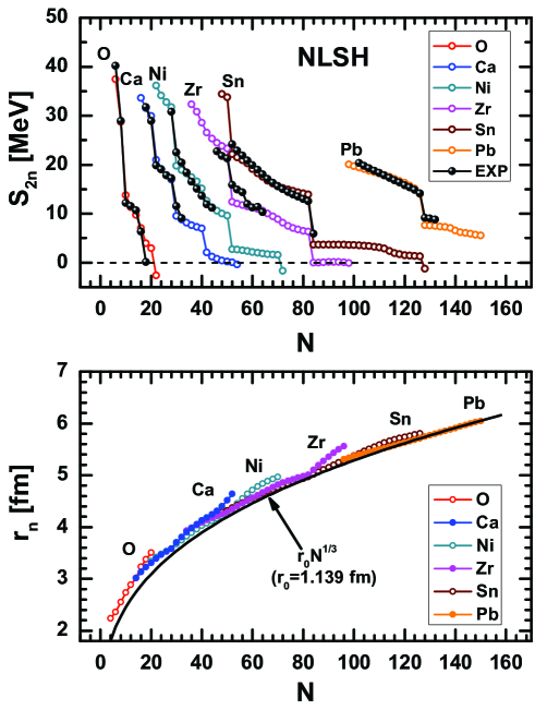
Figure 3: (Color online) (a) The two-neutron separation energies $S_{2{\rm n}}$ calculated by RCHB theory [39] with NLSH [153] (Open symbols) in comparison with data available (solid ones) for the even O, Ca, Ni, Zr, Sn, and Pb isotopes against the neutron number $N$. (b) The root mean square (rms) neutron radii $r_{n}$ for even O, Ca, Ni, Zr, Sn, and Pb isotopes by RCHB calculations against the neutron number $N$. The curve $r_{0}N^{1/3}$ with $r_{0}=1.139$ fm has been included to guide the eye. Taken from Ref. [29] with modified color.

In Fig. 3, similar to Ref. [29], the two-neutron separation energies $S_{\rm 2n}$ and the neutron radii $r_{n}$ from the RCHB calculation for the even-even nuclei of the O, Ca, Ni, Zr, Sn, and Pb isotope chains have been shown. The predicted $r_{n}$ curve using the simple empirical equation $r_{n}=r_{0}N^{1/3}$ with $r_{0}=1.139$ fm normalizing to ²⁰⁸Pb is also represented in the figure. This simple formula for $r_{n}$ agrees with the calculated neutron radii with exceptions in neutron rich Ca and Zr isotopes.

The comparison between experimental and calculated $S_{2{\rm n}}$ is shown in Fig. 3. The experimental magic or submagic numbers $N=20,28$, and $40$ are reproduced. The $S_{2{\rm n}}$ values for several nuclei in exotic Ca and Zr isotopes are extremely close to zero. As discussed in Refs. [28, 29], if taking ⁶⁰Ca or ¹²²Zr respectively as a core, the valence neutrons will gradually occupy the loosely bound states and the continuum above the sub-shell of $N=40$ in Ca or $N=82$ in Zr isotopes. Such typical behavior of $S_{2{\rm n}}$ can be taken as an evidence of the occurrence of giant halos in Ca chain and Zr chain [28].

In Fig. 3, it is very interesting to see that $r_{n}$ follows the $N^{1/3}$ systematics well for stable nuclei although their proton numbers are quite different. Near the drip line, distinct abnormal behaviors appear at $N=40$ in Ca isotopes and at $N=82$ in Zr isotopes. As pointed in Ref. [29], nuclei having the abnormal $r_{n}$ increase correspond to those having small $S_{2{\rm n}}$, which provides another evidence to the emergence of giant halos. The increase of $r_{n}$ in exotic Ni, Sn and Pb nuclei is not as rapid as those in Ca and Zr chains. The regions of the abnormal increases of the neutron radii are just the same as those for $S_{2n}$. Both behaviors are connected with the formation of giant halo [28, 29, 144, 145].

3.3 Halos from relativistic and non-relativistic approaches

By using the RCHB theory, predictions of halo in the Ne [38, 158], Na [101, 158], Ca [29] and Zr [28] isotopes near the neutron drip line have been made. In particular, in Ca and Zr isotopes near the neutron drip line, the halo phenomena were addressed as giant halo [28, 29]. In the non-relativistic HFB approaches, Skyrme calculations with the parameter set SLy4 predicted the halo in Sn and Ni [152]. It was also claimed that the pairing gaps have an effect to reduce the halo at the neutron drip line [152, 159, 160].

In Refs. [161, 162], the phenomena of the giant halo and halo of the neutron-rich even-Ca isotopes have been investigated and compared between the frameworks of the RCHB and the Skyrme HFB calculations. With the two parameter sets for each of the RCHB and the Skyrme HFB calculations, it has been found that although the halo phenomena exist for Ca isotopes near the neutron drip line in both calculations, the halo from the Skyrme HFB calculations (SkM*) starts at a more neutron-rich nucleus than that from the RCHB calculations, and SLy4 does not predict a halo, because the drip line is much closer to the stable region than the other parameter sets.

Figure 4: The neutron and proton rms radii $\bar{r}_{n}$ and $\bar{r}_{p}$ of even-Ca isotopes in RCHB calculations with NLSH and PK1 and the Skyrme HFB calculations with SkM^∗ and SLy4 in the neutron-rich region. Taken from Ref. [161].

Figure 4 shows systematics of the rms radii of neutrons $\bar{r}_{n}$ and protons $\bar{r}_{p}$ of even-Ca from $N=30$ to the two-neutron drip lines. The increase in the curvature of $\bar{r}_{n}$ indicates the halo. For Ca, the number of nucleons in continuum, $N_{h}$, of ^62-72Ca is 0.6–2.2, of which the average is 1.7, in the NL-SH calculation [29]; the corresponding value of the SkM^∗ calculation is always smaller than 0.5 (the average 0.27). As there are more than two halo neutrons, it was referred to as giant halo [28, 29]. The SkM^∗ calculation predicts the halo from $N=52$, and the RCHB calculations show the gradual occurrence of the giant halo. Apparently, the starting nucleus of the halo of SkM^∗ corresponds to the extra lowering of the $S_{2n}$. The SLy4 calculation does not predict the halo, because the particle-stable region ends at $N=46$. The large difference between $\bar{r}_{n}$ and $\bar{r}_{p}$ shown in Fig. 4 was identified as neutron skin in the region with no halo.

Figure 5: Radial wave function squared $|\psi_{r}|^{2}$ (canonical basis) of the neutron $3s_{1/2}$ of ⁶⁶Ca. They are normalized as $\int dr\,|\psi_{r}|^{2}=1$. Taken from Ref. [161].

The RCHB calculations have larger neutron rms radii systematically in $N\geq 40$ than the Skyrme HFB calculations. This difference comes partially from the occupation of the neutron $3s_{1/2}$ orbital, which causes 50% of the maximum difference in the neutron rms radii among the four calculations at ⁶⁶Ca. The difference in the neutron $3s_{1/2}$ orbital is shown in Fig. 5, which illustrates the radial wave functions squared. The tail of $3s_{1/2}$ from PK1 has appreciably extended distribution than the others, and as a consequence, the amplitude of PK1 is smaller in the inner region. The number and locations of the nodes are the same for the four curves.

As shown in the previous Subsection and in Ref. [28], the occupation of $3p_{1/2}$ and $3p_{3/2}$ orbitals are responsible for the formation of giant halos in Zr isotopes. In Ref. [163], the Hartree-Fock-Bogoliubov (HFB) approach with Skyrme interactions SLy4 and SkI4 has been used to study halos in Ca and Zr isotopes. It was found that the appearance of giant halos depends sensitively on the effective interaction adopted: SkI4 predicts a neutron halo in the Zr chain with $A\geq 122$ due to the weakly bound orbitals $3p_{1/2}$ and $3p_{3/2}$.

In the above mentioned work, the box boundary condition is adopted and the continuum is discretized. Although the convergence of the halo properties with respect to the box size has always been achieved, it is still desirable to examine the influence of the asymptotic behavior of the radial wave functions of those valence orbitals on the formation of halo or giant halo. The Skyrme HFB equations in $r$ space have been solved for spherical systems with correct asymptotic boundary conditions for the continuous spectrum [164] or the Green’s function technique [55, 57]. In Ref. [164], it was shown that close to the drip line the amount of pairing correlations depends on how the continuum coupling is treated. In Ref. [55], it was found that, in even-even $N=86$ isotones in the Mo-Sn region, the $l=1$ broad quasiparticle resonances persist in feeling the pairing potential and contribute to the pairing correlation even when the widths are comparable with the resonance energy. In Ref. [56], the investigation of the pair correlation in the tail of the giant halo revealed that the asymptotic exponential behavior of the neutron pair condensate is dominated by nonresonant continuum states with low asymptotic kinetic energy.

3.4 Halos with relativistic Hartree-Fock-Bogoliubov theory in continuum

In spite of successes of RCHB theory, there are still a number of questions needed to be answered in the conventional CDFT, e.g., the contributions due to the exchange (Fock) terms and the pseudo-vector $\pi$-meson. Earlier attempts to include the exchange terms with relativistic Hartree-Fock (RHF) method led to underbound nuclei due to the missing of the meson self-interactions [165, 126]. For a long time, the RHF theory failed in a quantitative description of nuclear systems [166, 167, 168, 169, 170, 126, 171, 172]. With the development of the computational facilities and numerical techniques, the density dependent relativistic Hartree-Fock (DDRHF) theory has been developed and shown significant improvements in a quantitative description of nuclear phenomena [127, 78, 113, 173, 174, 175, 176, 177] with comparable accuracy. With a number of adjustable parameters comparable to those of RMF Lagrangians, the DDRHF theory can give a equally good description of nuclear systems without dropping the Fock terms. Furthermore, important features like the behavior of neutron and proton effective masses [178] can be interpreted.

In DDRHF theory [127], the tensor forces due to $\pi$ and $\rho$ meson exchanges can be naturally taken into account and have brought significant improvements on the consistent description of shell evolution [173, 179, 180, 181]. The relativistic Hartree-Fock-Bogoliubov (RHFB) theory in continuum with density dependent meson-nucleon couplings is developed in Refs. [107, 114]. In the descriptions of nuclear halos, by using the finite range Gogny force D1S in the pairing channel, systematic RHFBc calculations are performed both for stable and weakly bound nuclei. It is demonstrated that an appropriate description of both mean field and pairing effects can be obtained within RHFBc theory [107, 114].

In Fig. 6, the single-neutron separation energies $S_{n}$ of Sn isotopes from ¹⁰¹Sn to ¹³⁸Sn (left panels) and the single-proton separation energies $S_{p}$ of $N=82$ isotones from ¹³⁰Cd to ¹⁵³Lu (right panels) are given. The odd-even differences on the single-nucleon separation energies reflect the effects of the pairing correlations. In Fig. 6, RHFBc with PKA1 [113] and PKO1 [127] as well as RHB with DD-ME2 [182] present comparable and satisfied quantitative agreements with the data for both isotopes and isotones. From Fig. 6, one can find some systematics in the results. On the neutron rich side, i.e., after ¹³²Sn for Sn isotopes and before ${}_{~{}64}^{146}$Gd for $N=82$ isotones, PKA1 shows better agreements than PKO1 and DD-ME2. This is mainly due to the improvements in the shell structures with exchange terms included, especially the shell closures beyond 50 and 82, i.e., 58 and 92, which may change the level density and then influence the pairing effects. On the proton rich side, these three approaches provide comparable agreement with the data.

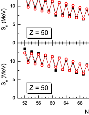
Figure 6: (Color online) Single-nucleon separation energies along Sn isotopic ($S_{n}$: left panels) and $N=82$ isotonic ($S_{p}$: right panels) chains. The results are calculated by RHFB with PKA1 [113], PKO1 [127], and by RHB with DD-ME2 [182], in comparison to the experimental data [183]. Taken from Ref. [114].

The Ce isotopes have been chosen to demonstrate the nuclear halo phenomenon within the RHFBc theory [107, 114]. In Fig. 7 the nuclear matter distributions (left panels) and neutron canonical single particle configurations (right panels) for Ce isotopes close to the drip line are shown. The neutron drip line calculated here with PKA1 [113] is $N=140$ whereas the calculations with PKO1 [127] and DD-ME2 [182] predict a shorter one as $N=126$. As shown in Fig. 7(a), the neutron densities become more and more diffuse after the isotope ¹⁸⁶Ce ($N=128$), a direct and distinct evidence of halo occurrence.

From Fig. 7(b) one can see that such extremely extensive matter distribution, e.g. in ¹⁹⁸Ce, is mainly due to the low-$l$ states, namely the halo orbitals $\nu 4s_{1/2}$, $\nu 3d_{5/2}$ and $\nu 3d_{3/2}$. From the occupations of the halo orbitals $N_{\rm halo}$ in Fig. 7(d), the halos were predicted in ¹⁸⁶Ce, ¹⁸⁸Ce and ¹⁹⁰Ce and giant halos may appear in ¹⁹²Ce, ¹⁹⁴Ce, ¹⁹⁶Ce and ¹⁹⁸Ce because more than two neutrons are occupying the halo orbitals. Similar conclusions can be obtained from the neutron numbers lying beyond the sphere with the radius $r=10$ fm [$N_{r>10~{}\rm{fm}}$ in Fig. 7(d)], which is large enough (the neutron matter radius $r_{n}=6.2$ fm in ¹⁹⁸Ce) for halos. Even extending to $r=16$ fm, which is sometime taken as the radial cut-off in the calculations of stable nuclei, there are still some amount of neutrons lying beyond this sphere in the isotopes from ¹⁹²Ce to ¹⁹⁸Ce.

In Fig. 7(c), one finds that the halo orbitals ($\nu 4s_{1/2}$, $\nu 3d_{5/2}$ and $\nu 3d_{3/2}$) are located around the particle continuum threshold where they are gradually occupied. For the isotopes beyond ¹⁸⁴Ce ($N=126$), the Fermi levels (in open circles) approach the continuum threshold rather closely such that the stability of these halo isotopes becomes sensitive to pairing effects. Nearby the low-$l$ states, there are the high-$l$ states $\nu 2g_{9/2}$ and $\nu 2g_{7/2}$. Because of the relatively large centrifugal barrier for $g$-orbitals they do not contribute much to the diffuse neutron distributions. Nevertheless, the existence of the high-$l$ states nearby halo orbitals is still particulary significant, because it leads to a rather high level density around the Fermi surface, and evidently the pairing effects are enhanced to stabilize the halo isotopes.

Figure 7: (Color online) (a) Neutron and proton densities, (b) the relative contributions of different orbitals to the full neutron density in ¹⁹⁸Ce, (c) neutron canonical single particle energies occupation probability (in $x$-error bars) and Fermi energy $E_{F}$ (in open circles), and (d) neutron numbers filling in the halo orbitals $4s_{1/2}$, $3d_{5/2}$, and $3d_{3/2}$ ($N_{\rm halo}$), and the ones lying beyond the spheres with the radii $r=10$, 11, 12, 13, 14, 15, 16 fm, respectively $N_{r>10\ {\rm fm}}$, $N_{r>11\ {\rm fm}}$, $N_{r>12\ {\rm fm}}$, $N_{r>13\ {\rm fm}}$, $N_{r>14\ {\rm fm}}$, $N_{r>15\ {\rm fm}}$ and $N_{r>16\ {\rm fm}}$. The results are calculated by RHFB with PKA1 [113] plus the Gogny pairing force D1S [124]. The spherical box radius is adopted as $R=28$ fm. Taken from Ref. [107].

Evidence for the existence of a halo can also be investigated by the systematic behavior of nuclear bulk properties such as radii. In Fig. 8, the isospin dependence of the neutron skin thickness ($r_{n}-r_{p}$) calculated in density dependent RHFB theory in continuum using PKA1 for Ca, Ni, Zr, Sn, and Ce isotopes are given [107]. Taking the stable nuclei as references (shown as the dashed lines), continuously growing deviations are found in the Ca, Zr, and Ce chains until the neutron drip line. This can be considered as evidence of a halo. Despite the deviations in the mid-region, both Ni and Sn nuclei show a similar isospin dependence in both stable and exotic nuclei regions, which indicate a neutron skin since the growth of a halo is interrupted. Compared with Ni, the Sn isotopes show even a much weaker skin effect.

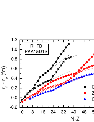
Figure 8: (Color online) Neutron skin thickness $r_{n}-r_{p}$ for Ca, Zr, Ni, Sn, and Ce as a function of the isospin ($N-Z$). The $r_{n}$ and $r_{p}$ are respectively the neutron and proton root mean square radii. The results are calculated by RHFB with PKA1 [113] plus the paring force D1S [124]. Taken from Ref. [107].

The systematics for the Ca and Zr chains from the RHFBc calculations are similar to those from the RCHB calculations [29]. For the Ce isotopes, RHFBc calculations with PKA1 show clear evidence for the existence of halo structures. The calculations of RHFBc with PKO1 [127] and RCHB with DD-ME2 [182] predict that the isotopic chain ends at $N=126$, before the halo occurrence as predicted by RHFB with PKA1. This deviation is interpreted by the shell structure evolution in Fig. 7(c), where much weaker shell are predicted with PKA1 in comparison with PKO1 and DD-ME2. As shown in Fig. 7(c), the neutron shell gap ($N=126$) between $\nu 1i_{13/2}$ and $\nu 2g_{9/2}$ states is close to the particle continuum threshold, which might essentially influence the stability of the drip line isotopes.

From Ref. [107], one may conclude that the Fock term itself has little direct impact on the formation of a nuclear halo. However, the Fock term may influence the shell structure, particularly those orbitals close to the Fermi surface in drip-line nuclei, thus affecting indirectly the formation of a potential halo.

3.5 Halos in exotic hyper nuclei

Motivated by knowledge of $\Lambda$-N interaction and understanding on giant halo [28, 29, 145], it is interesting to study the possible appearances of halos in exotic hyper nuclei.

Two neutron separation energies $S_{2n}$ for normal nuclei, single-$\Lambda$ hyper nuclei and double-$\Lambda$ hyper nuclei of Ca isotopes, labelled by $\Lambda=0$, $\Lambda=1$ and $\Lambda=2$, respectively, from the proton drip line to neutron drip line were investigated [104]. It was found that one or two $\Lambda$ hyperons lower the Fermi level due to the attractive $\Lambda$-N potential but keep the neutron shell structure unchanged. Therefore, the neutron drip line is pushed outside from $N=52$ in Ca isotope chain to $N=54$ in hyper isotope chain. Meanwhile, giant halos due to pairing correlation and the contribution from the continuum still exist in Ca hyper nuclei similar to that in Ca isotopes [29]. This is a slight but rewarding step for exploring the limit of drip line nuclei on the basis of the giant halo. For more details, see Ref. [104].

Apart from neutron halos in hyper nuclei, as $\Lambda$ hyperon is less bound than the corresponding nucleon in nuclei, it is worth investigating the existence of hyperon halos.

In Ref. [184, 185], a $\Lambda$ halo was tentatively suggested in a RMF plus BCS model. However, since the normal BCS method will have unphysical solution by involving baryon gas [39], such prediction needs further study. In Ref. [103], hyper carbon isotopes are studied by the RCHB theory. By investigating the baryon density distributions in hyper nuclei ${}^{13}_{\Lambda}$C, ${}^{14}_{2\Lambda}$C, and ${}^{15}_{3\Lambda}$C, it was found that with up to two $\Lambda$ hyperons added to the core ¹²C, the nucleon density distributions remain the same and hyperon density distributions at the tail are comparable with those of the nucleons. An intriguing phenomenon appears in ${}^{15}_{3\Lambda}$C where the hyperon density distribution has a long tail extended far outside of its core ${}^{14}_{2\Lambda}$C. This is a signature of hyperon halo due to the weakly bound state $1p_{3/2}^{\Lambda}$ in ${}^{15}_{3\Lambda}$C which has a small hyperon separation energy and a density distribution with long tail [103].

4 Surface diffuseness

From the mean field point of view, the properties of nucleons in an atomic nucleus are determined by the mean potential which stems from their interaction with the other nucleons and is determined by nucleon densities in the self-consistent models. Therefore, the study of the isospin dependence of the mean potential and the density distribution, both become highly diffuse near the particle drip line, is crucial to understand exotic nuclei. For finite nuclei, the diffuseness of the nuclear surface provides a measure of the thickness of the surface region. The surface diffuseness is intimately related to the spin-orbit splitting [142], the evolution of single particle shell structure [28], the pseudospin symmetry [76, 77, 186] and spin symmetry [83, 186], and the nuclear surface energy and thus nuclear masses [187]. In this Section, we will review recent progresses on nuclear surface diffuseness and the corresponding impact on nuclear shell structure and size.

4.1 Spin-orbit splitting and shell structure

The RCHB theory has been used to systematically study the isospin dependence of the mean potential for the Sn isotopes from proton drip line to neutron drip line and the spin-orbit splitting for the whole isotope chain was examined in details [142]. As an example, the spin-orbit splitting

$$E_{ls}=\displaystyle\frac{E_{lj=l-1/2}-E_{lj=l+1/2}}{2l+1}$$ (79)

versus the binding energy:

$$E=\displaystyle\frac{(l+1)E_{lj=l-1/2}+lE_{lj=l+1/2}}{2l+1}$$ (80)

in ^ASn with $A=110,120,\cdots,170$ are given in Fig. 9 for the neutron spin-orbit partners ($1d_{3/2},1d_{5/2}$), ($1g_{7/2},1g_{9/2}$), ($1i_{11/2},1i_{13/2}$), ($1p_{1/2},1p_{3/2}$), ($1f_{5/2},1f_{7/2}$) and ($1h_{9/2},1h_{11/2}$), and the proton spin-orbit partners ($1d_{3/2},1d_{5/2}$) and ($1f_{5/2},1f_{7/2}$).

It is very interesting to see that the spin-orbit splittings for the neutron and proton are very close to each other, at least for ($1d_{3/2},1d_{5/2}$) and ($1f_{5/2},1f_{7/2}$) cases. The splitting decreases monotonically from the proton drip line to the neutron drip line. To understand its mechanism, it is very helpful to examine the origin of the spin-orbit splitting in the Dirac equation.

For the Dirac nucleon moving in scalar and vector potentials, its equation of motion could be de-coupled and reduced for the upper component and the lower component, respectively. For the spin-orbit splitting, the Dirac equation can be reduced for the upper component as following:

$$[\frac{d^{2}}{dr^{2}}-\frac{1}{E+2M-\Sigma_{0}+\Sigma_{S}}\frac{d(2M-\Sigma_{0}+\Sigma_{S})}{dr}\frac{d}{dr}]G^{lj}_{i}(r)$$

$$- [\frac{\kappa(1+\kappa)}{r^{2}}-\frac{1}{E+2M-\Sigma_{0}+\Sigma_{S}}\frac{\kappa}{r}\frac{d(2M-\Sigma_{0}+\Sigma_{S})}{dr}]G^{lj}_{i}(r)$$

$$= - (E+2M-\Sigma_{0}+\Sigma_{S})(E-\Sigma_{0}-\Sigma_{S})G^{lj}_{i}(r).$$ (81)

The spin-orbit splitting is due to the corresponding spin-orbit potential

$$\frac{1}{E+2M-\Sigma_{0}+\Sigma_{S}}\frac{\kappa}{r}\frac{d(2M-\Sigma_{0}+\Sigma_{S})}{dr}$$ (82)

with some proper normalization factor. The spin-orbit splitting is energy dependent and depends on the derivative of the potential $2M-\Sigma_{0}+\Sigma_{S}$. Therefore the so-called spin-orbit potential, $V_{ls}=\displaystyle\frac{\kappa}{r}\frac{d(2M-\Sigma_{0}+\Sigma_{S})}{dr}$, is introduced.

Figure 9: The neutron spin-orbit splitting $E_{ls}=(E_{lj=l-1/2}-E_{lj=l+1/2})/(2l+1)$ versus the mass number $A$ in Sn isotopes for neutron ($1d_{3/2},1d_{5/2}$), ($1g_{7/2},1g_{9/2}$), ($1i_{11/2},1i_{13/2}$), ($1p_{1/2},1p_{3/2}$), ($1f_{5/2},1f_{7/2}$) and ($1h_{9/2},1h_{11/2}$) orbitals and proton ($1d_{3/2},1d_{5/2}$) and ($1f_{5/2},1f_{7/2}$) orbitals, respectively. Taken from Ref. [142].

The derivatives of the neutron potentials $\Sigma_{0}(r)-\Sigma_{S}(r)$ for ¹¹⁰Sn, ¹⁴⁰Sn, and ¹⁷⁰Sn, are given in the upper panel of Fig. 10. For both proton and neutron, the derivatives of the potentials $\Sigma_{0}(r)-\Sigma_{S}(r)$ are almost the same. As the potential $\Sigma_{0}-\Sigma_{S}$ is a big quantity ($\sim 700$ MeV), the isospin dependence in the spin-orbit potential could be neglected. That is the reason why the spin-orbit splitting for the neutron and proton is very close to each other in Fig. 9. From ¹¹⁰Sn to ¹⁷⁰Sn, the amplitude of the derivative for $\Sigma_{0}-\Sigma_{S}$ decreases monotonically due to the surface diffuseness.

Figure 10: Upper: The derivative of the neutron potentials $\Sigma_{0}(r)-\Sigma_{S}(r)$ for ^ASn with $A=110,120,\cdots,170$; Lower: The neutron potentials $\Sigma_{0}(r)-\Sigma_{S}(r)$ for ^ASn with $A=110,120,\cdots,170$. In order to examine the surface diffuseness more clearly, the radii $R_{0}$ at which $\Sigma_{0}(R_{0})-\Sigma_{S}(R_{0})=100$ MeV has been given as an inserted figure. Taken from Ref. [142].

The decline of the spin-orbit splitting is from the diffuseness of the potential or the outwards tendency of the potential. The neutron and proton potentials $\Sigma_{0}+\Sigma_{S}$ are given in Fig. 11 for ^ASn with $A=110,120,\cdots,170$. It is seen that the depth of the neutron potential decreases monotonically from the proton drip line to the neutron drip line and the surface moves outwards. The inserted figures give the radii $R_{0}$ at which $\Sigma_{0}+\Sigma_{S}=-10$ MeV as functions of the mass number. With the increase of the neutron number, the depth of the proton potential increases monotonically but is pushed towards outside as well due to the proton-neutron interaction.

Figure 11: Left: The neutron potentials $\Sigma_{0}(r)+\Sigma_{S}(r)$ for ^ASn with $A=110,120,\cdots,170$. In order to examine the surface diffuseness more clearly, the radii $R_{0}$ at which $\Sigma_{0}(R_{0})+\Sigma_{S}(R_{0})=-10$ MeV has been given as an inserted figure; Right: The proton potentials $\Sigma_{0}(r)+\Sigma_{S}(r)$ for ^ASn with $A=110,120,\cdots,170$. In order to examine the surface diffuseness more clearly, the radii $R_{0}$ at which $\Sigma_{0}(R_{0})+\Sigma_{S}(R_{0})=-10$ MeV has been given as an inserted figure. Taken from Ref. [142].

Similar neutron potentials $\Sigma_{0}-\Sigma_{S}$ for ^ASn with $A=110,120,\cdots,170$ are given in the lower panel of Fig. 10 and its inserted figure gives the radii $R_{0}$ at which $\Sigma_{0}-\Sigma_{S}=100$ MeV as a function of the mass number. As seen above, the spin-orbit splitting is related with the derivative of the potential $\Sigma_{0}-\Sigma_{S}$. The surface diffuseness happens for both the vector and scalar potential as shown in both $\Sigma_{0}-\Sigma_{S}$ and $\Sigma_{0}+\Sigma_{S}$.

Similar RCHB calculations have been carried out for all the nuclei in Na isotopes with mass number $A$ ranging from 17 to 45 with effective interaction NLSH [28]. Apart from the diffuseness of the potential, the shell evolution with neutron number has been examined there as well. In Fig. 12, the microscopic structure of the single particle energies in the canonical basis [188, 39] is given. In the left panel of Fig. 12, the single particle levels in the canonical basis for the Na isotopes with an even neutron number are shown. The level density becomes dense with the neutron number due to the decrease of the spin-orbit potential or diffuseness of the potential. Going from $A=19$ to $A=45$, it can be observed a big gap above the $N=8$, $N=20$ major shell, and $N=14$ sub-shell. The $N=28$ shell for stable nuclei fails to appear, as the $2p_{3/2}$ and $2p_{1/2}$ come so close to $1f_{7/2}$. When $N\geq 20$, the neutrons are filled to the levels in the continuum or weakly bound states in the order of $1f_{7/2}$, $2p_{3/2}$, $2p_{1/2}$, and $1f_{5/2}$. In the right part, the occupation probabilities in the canonical basis of all the neutron levels below $E=10$ MeV have been given for ³⁵Na to show how the levels are filled in nuclei near the drip line. The importance of careful treatment of the pairing correlation and the scattering of particle pairs to higher lying levels are noted in the figure.

Figure 12: Left part: Single particle energies for neutrons in the canonical basis as a function of the mass number for Na isotopes. The dashed line indicates the chemical potential. Right part: The occupation probabilities in the canonical basis for ³⁵Na. Taken from Ref. [101].

4.2 Interaction cross section

The neutron and proton distributions and radii are fundamental quantities to define the halo phenomena. However, the radius for unstable nucleus is normally extracted from the interaction cross sections by assuming an empirical form (e.g., a Gaussian function) for the density distribution [24]. It would be better to use the density distribution from the self-consistent models and calculate the interaction cross sections directly from Glauber model.

Such systematic calculations have been carried out for all the nuclei in Na isotopes with mass number $A$ ranging from 17 to 45 with the RCHB theory and the effective interaction NLSH [101]. The calculated binding energies $E$ and the interaction cross sections with the Glauber model are shown in Fig. 13. The calculated binding energies $E$ are compared with the empirical values [189]. The proton (neutron) drip line nucleus has been predicted to be ¹⁹Na (⁴⁵Na). The difference between the calculations and the empirical values for the stable isotopes is from the deformation, which has been neglected in Ref. [101].

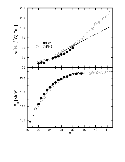
Figure 13: Upper part: The interaction cross sections $\sigma_{I}$ of ^ANa isotopes on a carbon target at $950A$ MeV: the open circles are the result of RCHB calculation and the available experimental data ($A=$20–23, 25–32) are given by solid circles with their error bars. The dashed line is a simple extrapolation based on the RCHB calculation for ^28-31Na. Lower part: Binding energies for Na isotopes, the convention is the same as the upper part, but the RCHB result for particle unstable isotopes are indicated by triangle. Taken from Ref. [101].

As the interaction cross sections $\sigma_{I}$ is well reproduced, the density distributions of the whole isotopes from the RCHB theory have been examined and the relation between the development of halo and shell effect has been studied in detail [101]. It was found that the neutron $N=28$ shell closure fades due to the lowering of the $2p$ orbitals. The tail in the nuclear density profile depends strongly on the shell structure and the development of a halo was connected with the changes in the occupation in the next shell or sub-shell close to the continuum limit [101].

Similar calculations have been performed for C, N, O and F isotopes up to the neutron drip line by the self-consistent RCHB theory [143]. The agreement between the calculated one neutron separation energies $S_{n}$ and the available experimental values are similar as Na isotopes. A Glauber model calculation for the total charge-changing cross section has been carried out with the density distribution obtained from the RCHB theory. The measured cross sections for studied nuclei with ¹²C as a target are nicely reproduced. An important conclusion was found that, contrary to the usual impression, the proton density distribution is less sensitive to the neutron number along the isotope chain. Instead it is almost unchanged from stability to the neutron drip line. Such calculations are quite useful in extracting both the proton and neutron distributions inside the nucleus and in defining the neutron/proton skin or halo.

4.3 Surface diffuseness correction in global mass formula

For finite nuclei, the diffuseness of nuclear surface is an important degree-of-freedom in the calculations of nuclear masses [187]. The density distributions of most stable nuclei are of the “neutron skin-type”, with a typical value around $0.5$ fm for the surface diffuseness. For nuclei near the neutron drip line, halos and giant halos may develop and the neutrons may distribute more extensive spatially than the protons, which implies the enhanced neutron surface diffuseness for these extremely neutron-rich nuclei. However, in global mass calculations, the surface diffuseness of exotic nuclei near the drip lines has not been properly considered. Recently, the surface diffuseness from the RCHB theory and its impact on the symmetry energy and shell correction have been studied in Ref. [187] and the accuracy of the global mass formula has been considerably improved.

Inspired by the Skyrme energy-density functional, a macroscopic-microscopic mass formula, the Weizsäcker-Skyrme (WS) formula [190, 191, 192], was proposed with a rms deviation around 336 keV with respect to the 2149 measured masses [183] in 2003 Atomic Mass Evaluation (AME). The WS models provide the best accuracy for nuclear masses in several mass regions [193, 194] and has been used in r-process simulations [195, 196].

In the WS formula, an axially deformed Woods-Saxon potential, with a contant surface diffuseness parameter $a$ for all nuclei, was used to obtain the single particle levels of nuclei. In Ref. [187], by taking into account the surface diffuseness correction for unstable nuclei, a new global mass formula, WS4, has been proposed. The surface diffuseness $a$ of the Woods-Saxon potential was given by $a=a_{0}\left(1+2\varepsilon\delta_{q}\right)$, with $\varepsilon=(I-I_{0})^{2}-I^{4}$ the correction factor for surface diffuseness, $a_{0}$ the diffuseness of the Woods-Saxon potential, $I_{0}=0.4A/(A+200)$ the isospin asymmetry of the nuclei along the $\beta$-stability line described by Green’s formula, and $\delta_{q}=1$ for neutrons (protons) in the nuclei with $I>I_{0}$ ($I<I_{0}$) and $\delta_{q}=0$ for other cases. This means that the surface diffuseness of neutron distribution is larger than that of protons at the neutron-rich side and smaller than that of protons at the proton-rich side. The rms deviation with the available mass data [197] falls to 298 keV, crossing for the first time the 0.3 MeV accuracy threshold for mass formulas (models) within the mean field framework.

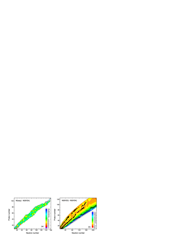
Figure 14: (Color online) (a) Difference between measured and the WS4 calculated masses. (b) Difference between WS3 and WS4 calculated masses. The squares and crosses denote the nuclei first appearing in AME2012 and the nuclei with $|I-I_{0}|>0.1$, respectively. The smooth and the zigzag curves denote the $\beta$-stability line from the Green’s formula and the neutron drip line from the WS4 formula, respectively. Taken from Ref. [187].

In Fig. 14(a), it was shown the deviations of the calculated masses from the experimental values. For all the 2353 nuclei with $Z$ and $N\geq 8$, the deviation is within 1.23 MeV. In Fig. 14(b), the difference between the WS3 (constant surface diffuseness $a_{0}$) and WS4 calculated masses. For most nuclei, the results of WS3 and WS4 are consistent in general (with deviations smaller than one MeV). For nuclei near the neutron drip line, the masses given by WS4 are larger than the results of WS3 by several MeV. This is due to the enhancement of the nuclear symmetry energy coming from the surface diffuseness effect in the extremely neutron-rich nuclei.

It is worthwhile to note that with an accuracy of 258 keV for all the available neutron separation energies and of 237 keV for the alpha-decay $Q$-values of superheavy nuclei, the proposed mass formula will be important not only for the reliable description of the r-process of nucleosynthesis but also for the study of the synthesis of superheavy nuclei.

5 Pairing correlations and nuclear size

In Ref. [159], it is shown that the neutron ground state Hartree-Fock (HF) asymptotic density equals

$$\rho(r)\propto\exp{(-2\mu r)/r^{2}},$$ (83)

with $\mu=\sqrt{-2m\varepsilon_{k}}/\hbar$ and $\varepsilon_{k}$ the single particle energy of the least bound $l=0$ neutron. The corresponding mean square radius deduced from the asymptotic solution is

$$\langle r^{2}\rangle_{\mathrm{HF}}\propto\frac{\hbar^{2}}{2m|\varepsilon_{k}|},$$ (84)

which diverges in the limit $\varepsilon_{k}\rightarrow 0$.

In the presence of pairing, the mean square radius deduced from the asymptotic Hartree-Fock-Bogoliubov (HFB) density is

$$\langle r^{2}\rangle_{\mathrm{HFB}}\propto\frac{\hbar^{2}}{2m(E_{k}-\lambda)}$$ (85)

with the lowest discrete quasiparticle energy $E_{k}=\sqrt{(\varepsilon_{k}-\lambda)^{2}+\Delta_{k}^{2}}$. If the pairing gap $\Delta_{k}$ is finite, the radius will never diverge in the limit of small separation energy $\varepsilon_{k}\simeq\lambda\rightarrow 0$.

The asymptotic HF and HFB densities characterized by $l=0$ orbitals were compared in Ref. [159] and it has been emphasized that pairing correlations reduce the nuclear size and an extreme halo with infinite radius cannot be formed in superfluid nuclear systems. Here pairing correlations act against the formation of an infinite radius. Therefore this effect was called “pairing anti-halo effect” in Ref. [159].

In fact, the mechanism leading to a halo in Eq. (84), i.e., the valence nucleons occupy the weakly-bound orbital below and very close to the continuum threshold, has been used in early interpretation for nuclear halo phenomena [146, 147, 96]. The limiting condition $\varepsilon_{k}\rightarrow 0$ and the radius deduced from this $l=0$ orbital alone correspond to an extremely ideal situation, which is difficult to be found in real nuclei.

In Ref. [198], the influences of pairing correlations on the nuclear size and on the development of a nuclear halo were studied in details by the self-consistent RCHB theory [39]. In order to simplify the problem, neutron-rich nuclei with the neutron Fermi surface below, between and above two weakly-bound $2p$ levels are investigated with a fixed Wood-Saxon potential, which is followed by the self-consistent calculation on the well studied neutron halos in ¹¹Li and ³²Ne with low-$l$ orbitals in the continuum.

5.1 Fermi surface and nuclear size

In order to investigate the impact of nuclear binding on nuclear size for varying pairing potential, a spherical Woods-Saxon shape mean field potential fitted to the corresponding neutron potentials resulting from a self-consistent calculation for ⁴²Mg is adopted [198].

The total neutron radius of the nucleus is given by

$$R_{N}=\frac{1}{N}\sum_{nlj}(2j+1)\,\langle r\rangle_{nlj}\,v^{2}_{nlj},$$ (86)

which is determined by the rms radii of the orbitals $\langle r\rangle_{nlj}$ and the corresponding occupation probabilities $v^{2}_{nlj}$.

Figure 15: (Color online) Single neutron levels $2p$ and $1f$ near the Fermi surface in the canonical basis, the rms radii $\langle r\rangle_{nlj}$, occupation probabilities $v^{2}_{nlj}$, contributions $v^{2}_{nlj}\times\langle r\rangle_{nlj}$ to the neutron rms radii, and the total neutron rms radii $R_{N}$ for $N=28,~{}30,~{}32$, and $34$ as a function of average pairing gap $\Delta$. The Fermi surfaces for the neutron numbers are plotted as dashed lines. Taken from Ref. [198].

In Fig. 15, the single neutron levels $\varepsilon_{k}$ in the canonical basis [188], the rms radii $\langle r\rangle_{nlj}$, the occupation probabilities $v^{2}_{nlj}$, the contributions $v^{2}_{nlj}\times\langle r\rangle_{nlj}$ to the neutron rms radius for the orbitals near the Fermi surface ($2p$ and $1f$), and the total neutron rms radii $R_{N}$ for four neutron-rich Mg isotopes with $N=28,~{}30,~{}32$, and $34$ are plotted as functions of the pairing gap

$$\Delta=\frac{1}{N}\sum_{nlj}(2j+1)\Delta^{(lj)}_{n}v_{nlj}^{2}.$$ (87)

Here $\Delta^{(lj)}_{n}$ are the diagonal matrix elements of the pairing field in the canonical basis.

The single neutron levels in canonical basis are obtained by solving the corresponding RCHB equations for various pairing strength. In principle, the energy levels $\varepsilon_{nlj}=h^{(lj)}_{nn}$ depend on $\Delta$. However, since this solution was obtained for fixed WS potentials, as shown in the upper panels of Fig. 15, these states remain almost unchanged with increasing pairing correlations.

For Mg isotopes with $N=28,~{}30,~{}32$, and $34$, the neutron Fermi surface (shown as dashed line in upper panels of Fig. 15) is located just below the two weakly-bound $2p$ levels, between them, crossing the $2p_{1/2}$ level, and above the $2p$ levels. As the pairing strength increases, more neutrons are scattered from occupied levels in the Fermi sea to empty levels above the Fermi level, and therefore the Fermi surface is raising.

In Fig. 15, the rms radii of the $2p$ orbitals are much larger than those of the $1f$ orbitals due to the lower centrifugal barrier. With increasing pairing correlations, the rms radius decreases for $2p$ and $1f$ levels. This is the so-called “pairing anti-halo effect” discussed in Ref. [159]. However, this effect concerns only the radii $\langle r\rangle_{nlj}$ of the individual orbitals. The total neutron radius of the nucleus in Eq. (86) is determined by the rms radii of the orbitals and the occupation probabilities, which depend strongly on the pairing correlations.

As shown in Fig. 15, for $N=28$ the neutron Fermi surface is just below the two weakly-bound $2p$ levels. Without pairing correlations, the occupation probability is $1.0$ for the $1f_{7/2}$ orbital, and it vanishes for the $2p$ and the $1f_{5/2}$ orbitals. As the pairing strength increases, the neutrons on $1f_{7/2}$ orbital are scattered to $2p$ and $1f_{5/2}$ orbitals which have much larger rms radii. Therefore, the contributions to the total neutron rms radius from $2p$ and $1f_{5/2}$ states grow more than the contribution from $1f_{7/2}$ state decreases. As a result, the total neutron rms radius increases monotonically, where the contributions from $2p$ orbitals play a dominant role.

For $N=30$ in Fig. 15, the $2p_{1/2}$ and the $1f_{5/2}$ orbitals are empty for zero pairing, while the $1f_{7/2}$ orbital is fully occupied and the $2p_{3/2}$ orbital is half occupied. With increasing pairing strength, the neutrons in the $1f_{7/2}$ orbital are scattered to the $2p$ orbitals which contribute strongly to the neutron rms radius. Therefore, the total neutron rms radius $R_{N}$ increases with the growing pairing strength up to $\Delta=0.9$ MeV. Increasing the pairing strength further, the neutrons are continuously to be scattered from the $1f_{7/2}$ to the $2p_{1/2}$ state, while the neutron number in the $2p_{3/2}$ orbital decreases slightly and the resonance state $1f_{5/2}$ begins to be occupied. Together with the monotonic decreasing rms radii of the individual orbitals, the increase resulting from the $2p_{1/2}$ and $1f_{5/2}$ states is smaller than the decreases of the contributions from the $2p_{3/2}$ and $1f_{7/2}$ states. Therefore, for very strong pairing correlations, the total neutron rms radius finally decreases. As it is clearly seen this decrease is not caused by the pairing anti-halo effect, because the radius of the $1f_{7/2}$ state stays completely constant. It has its origin in the reoccupation caused by pairing.

For $N=32$ in Fig. 15, the $1f_{7/2}$ and $2p_{3/2}$ orbitals are fully occupied without pairing correlations, while the $2p_{1/2}$ and $1f_{5/2}$ orbitals are empty. As the pairing strength increases, the neutrons in the $1f_{7/2}$ and $2p_{3/2}$ orbitals are scattered to the $2p_{1/2}$ orbital, whose rms radius is larger than the ones of $1f_{7/2}$ and $2p_{3/2}$ levels. The contribution of the $2p_{1/2}$ orbitals causes an increase in the total neutron rms radius up to a pairing gap $\Delta=0.9$ MeV. As the pairing strength continues to grow beyond this value, the neutrons in the $2p_{3/2}$ state begin to be scattered to the $1f_{5/2}$ state which provides a smaller contribution than the $2p_{3/2}$ state, while the occupation probability remains almost constant for the $1p_{1/2}$ state. Together with the decreasing rms radius of the individual orbitals, the total neutron rms radius finally decreases for very large pairing.

For $N=34$, the two weakly-bound $2p$ levels are fully occupied for zero pairing, and the Fermi surface is just above the weakly-bound $2p$ levels. With increasing pairing strength, the neutrons in the $1f_{7/2}$ and $2p$ orbitals are scattered to the $1f_{5/2}$ orbital with a much smaller rms radius than the $2p$ orbitals. The contributions to the total neutron rms radius from the $1f_{7/2}$ and $2p$ orbitals decrease more than the increase of the contribution from $1f_{5/2}$ orbital, and therefore the total neutron rms radius finally decreases monotonically. Here the two effects, decreasing rms radius of the individual orbitals and changes of the occupation probabilities, act in the same direction. The decrease of the total neutron radius $R_{N}$ with increasing pairing correlations is not only from the decreasing rms radii of the individual orbitals but also from the change of the occupation probabilities.

It is clear that pairing correlations can change the rms radii of the individual weakly-bound orbitals and simultaneously the corresponding occupation probabilities. As a result, they have an influence on the nuclear rms radius and the total nuclear size. Furthermore, the contributions of the weakly-bound $2p$ orbitals to the nuclear rms radius play an important role.

5.2 Crucial low $l$ orbitals

Following the investigation on the impact of nuclear binding on nuclear size, the next question is the impact of orbital binding on the nuclear size as a function of the pairing potential. In Ref. [198], this problem has been investigated for the orbitals $2p$ as well-bound, weakly-bound, around the continuum threshold, and in the continuum cases.

Figure 16: (a) Single neutron levels $1d_{3/2}$, $1f_{7/2}$, $2p_{3/2}$, $2p_{1/2}$, and $1f_{5/2}$ in WS potentials of varying depth with $\varepsilon_{2p_{1/2}}=-5.0,~{}-0.5,~{}0.0$, and $0.5$ MeV. (b) Changes of the total neutron rms radii $\delta R_{N}=R_{N}(\Delta)-R_{N}(\Delta=0)$ for the various cases of $\varepsilon_{2p_{1/2}}$ as a function of average pairing gap $\Delta$. The shadow area represents the results calculated with different box sizes in the WS potential for $\varepsilon_{2p_{1/2}}=0.5$ MeV. Taken from Ref. [198].

In Fig. 16(a), the single neutron levels $1d_{3/2},~{}1f_{7/2},~{}2p_{3/2},~{}2p_{1/2}$, and $1f_{5/2}$ for $N=28$ in WS potentials with varying depth such that $\varepsilon_{2p_{1/2}}=-5.0,~{}-0.5,~{}0.0$, and $+0.5$ MeV are shown. In Fig. 16(b), for each $\varepsilon_{2p_{1/2}}$, the change of the total neutron rms radius with respect to that of zero pairing, $\delta R_{N}=R_{N}(\Delta)-R_{N}(\Delta=0)$, is plotted as a function of the pairing gap.

For $\varepsilon_{2p_{1/2}}=-5.0$ MeV which corresponds to a well bound nucleus, the neutron rms radius $R_{N}(\Delta)$ increases slightly with the pairing gap increasing from $0.0$ to $1.5$ MeV. For $\varepsilon_{2p_{1/2}}=-0.5,~{}0.0,~{}+0.5$ MeV which correspond to a weakly-bound nucleus, increases by more than $0.1$ fm are observed. It has to be noticed that for $\varepsilon_{2p_{1/2}}=+0.5$ MeV, both levels $2p_{1/2}$ and $2p_{3/2}$ are in the continuum. If the pairing correlation is switched on, the system is basically not bound. The eigenvalue problem is solved in a finite box and the solution depends on the box size. As an illustration, when the box size changes from $20$ to $25$ fm, the neutron rms radius calculated with a box radius of $25$ fm is about $0.05$ fm larger than that obtained with with a radius of $20$ fm box for $\Delta=1.5$ MeV as shown as shadowed region in Fig. 16(b).

For the discussion on the influence of pairing correlations on the nuclear size so far, the mean fields are fixed in the form of spherical WS potentials, and only the pairing strength and the Fermi level for $N=28,~{}30,~{}32,~{}34$ are considered. Here, with the changing pairing strength and the Fermi level, the single neutron levels stay almost constant except slight modification by the pairing field. In Ref. [198], fully self-consistent RCHB calculation for neutron-rich nuclei ^40,42,44,46Mg has been performed, it should be emphasized that qualitatively the effect of pairing correlations on the nuclear size agrees with that found for fixed WS potentials.

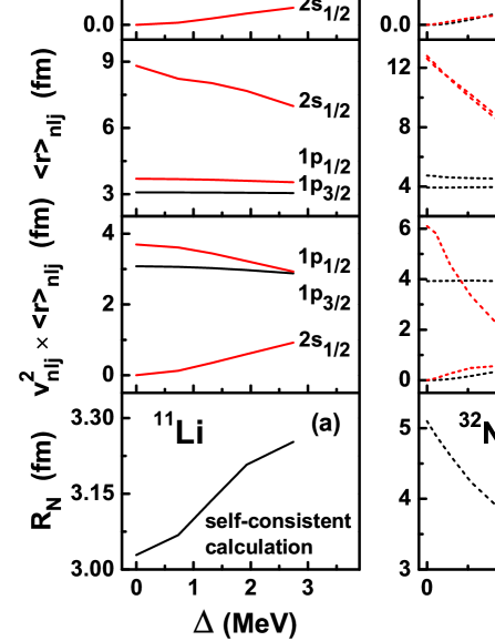
Figure 17: (Color online) Same as Fig. 15, but for ¹¹Li and ³²Ne. Taken from Ref. [198].

5.3 Pairing correlations and halos

In order to investigate the effect of pairing correlations on the development of a nuclear halo, self-consistent calculations are performed with different pairing strength for the well known neutron halo nuclei ¹¹Li [34] and ³²Ne [38], where the low-$l$ orbitals are in the continuum [198]. Single neutron levels in the canonical basis, the rms radii $\langle r\rangle_{nlj}$, the occupation probabilities $v^{2}_{nlj}$, the contributions to the neutron rms radius $v^{2}_{nlj}\times\langle r\rangle_{nlj}$, and the total neutron rms radii are plotted in Fig. 17 as a function of the average pairing gap for the nuclei ¹¹Li (panel a) and ³²Ne (panel b).

For ¹¹Li in Fig. 17(a), a halo is developed by scattering the neutrons to the $2s_{1/2}$ orbitals in continuum and the increasing pairing correlations will promote the development of this halo.

For ³²Ne in Fig. 17(b), the $2p$ and $1f_{7/2}$ orbitals are in the continuum. Without pairing correlations, the last two neutrons occupy the $2p_{3/2}$ orbital and therefore this nucleus is unbound and the rms radius depends on the box size. Increasing the pairing strength, the Fermi surface comes down and becomes negative when the pairing gap gets larger than $1.0$ MeV. It shows that for the halo nuclei such as ³²Ne, where the low-$l$ orbitals are in the continuum and unoccupied without pairing correlation, increasing pairing correlations will decrease the size of the nuclear halo, but nonetheless pairing plays an essential role: Without pairing the nucleus would stay unbound.

It is concluded that the weakly-bounded orbitals with low orbital angular momenta $l$ in the neighborhood of the threshold to the continuum play an important role [198]. The pairing correlations have a two-fold influence on the total nuclear rms radius and the nuclear size. First, they can change the rms radii of individual weakly bound orbitals and, second, they can change the occupation probabilities of these orbitals. With increasing pairing strength, the individual rms radii are reduced (pairing anti-halo effect). Meanwhile pairing changes also the occupation probabilities. The total nuclear size is determined by the competition between this two effects.

In Ref. [198], the strength of the pairing correlations was an external variable parameter. In realistic nuclei, the strength of pairing depends on the level density in the vicinity of the Fermi surface. Therefore, even orbitals with high $l$-values and large centrifugal barriers can contribute indirectly to changes of the nuclear size [38]. If they come close to the Fermi surface, they enhance pairing correlations and influence at the same time the occupation of low-$l$ orbitals close to the continuum limit and therefore the nuclear size.

6 Deformed halo and shape decoupling

Most open shell nuclei are deformed. The interplay between deformation and weak binding raises interesting questions, such as whether or not there exist halos in deformed nuclei and, if yes, what are their new features. Calculations in a deformed single particle model [199] have shown that the valence particles in specific orbitals with low projection of the angular momentum on the symmetry axis can give rise to halo structures in the limit of weak binding. The deformation of the halo is in this case solely determined by the intrinsic structure of the weakly bound orbitals. Indeed, halos in deformed nuclei were investigated in several mean field calculations in the past [200, 201, 133]. In Ref. [202], it has been concluded that in the neutron orbitals of an axially deformed Woods-Saxon potential the lowest-$l$ component becomes dominant at large distances from the origin and therefore all $\Omega^{\pi}=1/2^{+}$ levels do not contribute to deformation for binding energies close to zero. Such arguments raise doubt about the existence of deformed halos. In addition, a three-body model study [203] suggested that it is unlikely to find halos in deformed drip line nuclei because the correlations between the nucleons and those due to static or dynamic deformations of the core inhibit the formation of halos.

Therefore a model which provides an adequate description of halos in deformed nuclei must include in a self-consistent way the continuum, deformation effects, large spatial distributions, and the coupling among all these features. In addition it should be free of adjustable parameters in order to make predictions reliable.

Over the past years, lots of efforts have been made to develop a deformed relativistic Hartree (RH) theory [135] and a deformed relativistic Hartree-Bogoliubov theory in continuum (DRHBc theory) [108]. As a first application, halo phenomena in deformed nuclei have been investigated within the DRHBc theory [30]. The detailed theoretical framework is available in Ref. [31]. The DRHBc theory is useful to answer questions concerning exotic nuclear phenomena in nuclei near the drip line [200, 199, 204, 140, 203, 201], such as whether there are deformed halos or not and what new features can be expected in deformed exotic nuclei. In Ref. [205], the DRHBc theory is extended to incorporate the blocking effect due to an odd nucleon. In such a way, pairing correlations, continuum, deformation, blocking effects, and extended spatial density distributions in exotic odd-$A$ or odd-odd nuclei can be taken into account microscopically and self-consistently. In recent years, the CDFT with the density-dependent meson-nucleon couplings have attracted more and more attention owing to improved descriptions of the equation of state at high density, the asymmetric nuclear matter and the isovector properties of nuclei far from stability. Therefore, it’s necessary to develop a density-dependent deformed relativistic Hartree-Bogoliubov (DDDRHB) theory in continuum. The challenge is the treatment on the density-dependent couplings, meson fields, and potentials in axially deformed system with partial wave method. Quite recently, the DDDRHB theory in continuum was developed in Ref. [109]. In this Section, the halo in deformed exotic nucleus and its mechanism as well as possible shape decoupling will be briefly reviewed.

6.1 Neutron separation energy and nuclear size

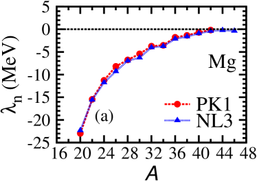
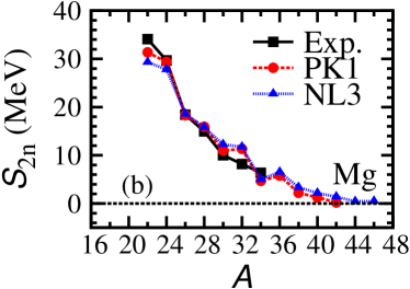
Figure 18: (Color online) The neutron Fermi energy $\lambda_{\mathrm{n}}$ (left panel) and two neutron separation energy $S_{\mathrm{2n}}$ (right panel) of Mg isotopes calculated by DRHBc theory with the parameter sets NL3 and PK1. The data of $S_{\mathrm{2n}}$ (labeled as “Exp.”) are taken from [183]. Taken from Ref. [31].

Figure 18 shows the neutron Fermi energy $\lambda_{\mathrm{n}}$ and two neutron separation energy $S_{\mathrm{2n}}$ of Mg isotopes calculated in the DRHBc theory with the parameter sets NL3 and PK1. Available data of $S_{\mathrm{2n}}$ taken from [183] are also included for comparison. Except the different prediction of the drip line nucleus, the neutron Fermi surfaces and two neutron separation energies from both parameter sets are very similar. The calculated two neutron separation energies $S_{2n}$ of Mg isotopes agree reasonably well with the available experimental values except for ³²Mg. The large discrepancy in ³²Mg is connected to the shape and the shell structure at $N=20$. For details, see Ref. [31].

Experimentally ⁴⁰Mg has been observed [206]. Theoretically there are different predictions on the last bound nucleus in Mg isotopes, e.g., ⁴⁴Mg from the finite range droplet model [207], ⁴⁰Mg from a macroscopic-microscopic model [208], a RMF model with the parameter set NLSH [209], and a Skyrme HFB model solved in a 3-dimensional Cartesian mesh [210], and ⁴²Mg from a Skyrme HFB model solved in a transformed harmonic oscillator basis [64] and the HFB21 mass table [211]. Therefore the prediction of the neutron drip line nucleus in Mg isotopes is model and parametrization dependent. In the DRHBc calculations with the parameter set NL3, ⁴⁶Mg is the last nucleus of which the neutron Fermi surface is negative and the two neutron separation energy is positive. However, with the parameter set PK1, ⁴²Mg is predicted to be the last nucleus within the neutron drip line.

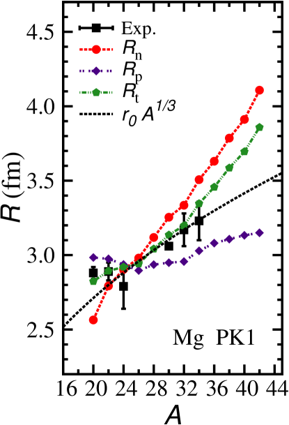
Figure 19: (Color online) The root mean square (rms) radii for Mg isotopes calculated in DRHBc theory plotted as functions of the neutron number. The neutron radii $R_{\rm n}$, proton radii $R_{\rm p}$, matter radii $R_{\rm t}$, the $r_{0}A^{1/3}$ curve, and the available data for $R_{\rm t}$ [212, 213] are given. The neutron radius $R_{\rm n}$, proton radius $R_{\rm p}$ and total radius $R_{\rm t}$ of Mg isotopes are calculated with PK1. The $r_{0}A^{1/3}$ curve is included to guide the eye. The data for matter radii labeled by “Exp.” are taken from Refs. [212, 213]. Taken from Ref. [31].

In Fig. 19, the rms radii for Mg isotopes are plotted as functions of the neutron number, including the neutron radii $R_{\rm n}$, proton radii $R_{\rm p}$, matter radii $R_{\rm t}$, the $r_{0}A^{1/3}$ curve, and the available data for $R_{\rm t}$ [212, 213]. The calculated matter radius follows roughly the $r_{0}A^{1/3}$ curve up to $A=34$. From ³⁶Mg on, the matter radius lies much high above the $r_{0}A^{1/3}$ curve. This indicates some exotic structure in these nuclei.

6.2 Density distributions and nuclear shape

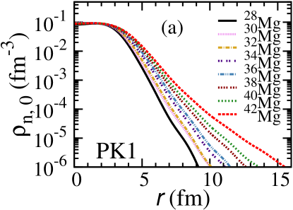
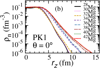
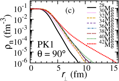
Figure 20: (Color online) Neutron density profiles of even-even Mg isotopes with $A\geq 28$ calculated in DRHBc theory with the parameter set PK1. The upper panel represents the spherical component of the neutron density distribution $\rho_{\mathrm{n},\lambda=0}(r)$. The middle panel refers to the density distribution $\rho_{\mathrm{n}}(z,r_{\perp}=0)$ along the symmetry axis $z$ ( $\theta=0^{\circ}$) with $r_{\perp}=\sqrt{x^{2}+y^{2}}$ and the lower panel refers to $\rho_{\mathrm{n}}(z=0,r_{\perp})$ that perpendicular to the symmetry axis $z$ ($\theta=90^{\circ}$). Taken from Ref. [31].

Figure 20 shows neutron density profiles of even-even Mg isotopes with $A\geq 28$ calculated in DRHBc theory with the parameter set PK1 [31]. The spherical component of the neutron density distribution is represented by $\rho_{\mathrm{n},\lambda=0}(r)$. The density distributions along the symmetry axis $z$ ($\theta=0^{\circ}$) and perpendicular to the symmetry axis $z$ ($\theta=90^{\circ}$) are respectively represented by $\rho_{\mathrm{n}}(z,r_{\perp}=0)$ and $\rho_{\mathrm{n}}(z=0,r_{\perp})$ with $r_{\perp}=\sqrt{x^{2}+y^{2}}$.

With increasing $A$, the spherical component of the neutron density distribution $\rho_{\mathrm{n},\lambda=0}(r)$ changes quickly at ³⁴Mg and abruptly at ⁴²Mg. The density distribution along the symmetry axis $\rho_{\mathrm{n}}(z,r_{\perp}=0)$ changes abruptly from ³²Mg to ³⁴Mg. This can be understood easily from the shape change in these two nuclei: ³²Mg is spherical but ³⁴Mg is prolate which means that it is elongated in the $z$ axis. In the direction perpendicular to the symmetry axis, the neutron density $\rho_{\mathrm{n}}(z=0,r_{\perp})$ of ⁴²Mg extends very far away from the center of the nucleus and a long tail emerges, revealing the formation of a halo.

By comparing $\rho_{\mathrm{n}}(z,r_{\perp}=0)$ and $\rho_{\mathrm{n}}(z=0,r_{\perp})$ for ⁴²Mg, it was found that in the tail part, the neutron density distributes more along the direction perpendicular to the symmetry axis. Since this nucleus as a whole is prolate, it indicates that the tail part has a different shape from the nucleus itself. This is the shape decoupling which was first predicted in Ref. [30].

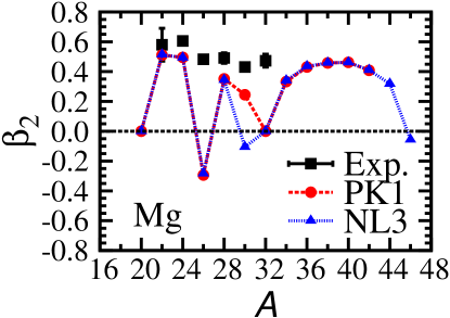
Figure 21: (Color online) The quadruple deformation parameter $\beta$ of Mg isotopes calculated with the parameter sets NL3 and PK1. The data labeled with “Exp.” are taken from [214]. Taken from Ref. [31].

The comparison of quadrupole deformation $\beta$ between the deformed RHB calculation and the experiment is given in Fig. 21. The experimental value of $\beta$ is extracted from the measured $B(E2:0^{+}_{1}\rightarrow 2^{+}_{1})$ and only the absolute value could be obtained [214]. The results of NL3 are almost the same as the results of PK1 except for ³⁰Mg. It is slightly oblate with NL3 but it has a prolate shape with PK1. For ³²Mg, the gap between the neutron levels $1d_{3/2}$ and $1f_{7/2}$ is almost $7$ MeV which results in a strong closed shell at $N=20$. Therefore the deformed RHB calculations with both parameter sets predict spherical shapes for this nucleus. This results in the large discrepancy in $S_{\mathrm{2n}}$ for ³²Mg as is seen in Fig. 18. Other mean field models also predict spherical or almost spherical shapes for ³²Mg [215, 209, 210, 216, 217]. However, this nucleus is well deformed as is indicated by the large $B(E2:0^{+}_{1}\rightarrow 2^{+}_{1})$ value [218]. The same is true for some neighboring nuclei with $N\sim 20$. These nuclei form the so called “island of inversion” [219, 220, 221, 222] which is related to the quenching of the $N=20$ shell closure. In order to describe the shell quenching effect at $N=20$, one has to go beyond the mean field [223, 217].

6.3 Deformed halo and shape decoupling

The deformed relativistic Hartree-Bogoliubov theory in continuum with the parameter set PK1 predicted the last bound neutron rich nucleus for Mg isotopes as ⁴²Mg [31]. There are both prolate and oblate stable solutions for ⁴²Mg. The ground state of ⁴²Mg is prolate. With the triaxially deformed relativistic mean field calculations [224], it is shown that the obtained oblate minimum is not an isomeric state but a saddle point in the potential energy surface.

It is found that the ground state of ⁴²Mg is well deformed with $\beta\approx 0.41$ and two neutron separation energy $S_{2n}\approx 0.22$ MeV [31]. The density distribution of such weakly bound nucleus has a very long tail in the direction perpendicular to the symmetry axis, see Fig. 20, which indicates the prolate ⁴²Mg has an oblate halo.

The density distribution is divided into contributions of the oblate “halo” and of the prolate “core” in Fig. 22. The density distribution of this weakly bound nucleus has a very long tail in the direction perpendicular to the symmetry axis which indicates the prolate nucleus ⁴²Mg has an oblate halo and there is a decoupling between the shapes of the core and the halo. It should be noted that in the calculations with NL3, ⁴⁶Mg is the last nucleus [30].

Figure 22: (Color online) Density distributions of the ground state of ⁴²Mg with the $z$ axis as the symmetry axis: (a) the neutron halo, and (b) the neutron core. Taken from Ref. [31].

The single particle spectrum around the Fermi level for the ground state of ⁴²Mg is shown in Fig. 23 [31]. The good quantum numbers of each single particle state are also shown. The occupation probabilities $v^{2}$ in the canonical basis have BCS-form [188] and are given by the length of the horizontal lines in Fig. 23. The levels close to the threshold are labeled by the number $i$ according to their energies, and their conserved quantum number $\Omega^{\pi}$ as well as the main spherical components are given at the right hand side. The neutron Fermi level is within the $pf$ shell and most of the single particle levels have negative parities. Since the chemical potential $\lambda_{n}$ is close to the continuum, orbitals above the threshold have noticeable occupations due to the pairing correlations. The single neutron levels of ⁴²Mg can be divided into two parts, the deeply bound levels ($\varepsilon_{\rm can}<-2$ MeV) corresponding to the “core”, and the remaining weakly bound levels close to the threshold ($\varepsilon_{\rm can}>-0.3$ MeV) and in the continuum corresponding to the “halo”.

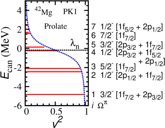
Figure 23: (Color online) Single neutron levels of ground state of ⁴²Mg in the canonical basis as a function of the occupation probability $v^{2}$. The blue dashed line corresponds to the BCS-formula with an average pairing gap. Taken from Ref. [31].

As discussed in Refs. [30, 31, 225], the shape of the halo originates from the intrinsic structure of the weakly bound or continuum orbitals. By examining the neutron density distribution, it was found that for the ground state of ⁴²Mg, the halo is mainly formed by level 4 and level 5. A detailed analysis of the intrinsic properties revealed that in ⁴²Mg the shape of the halo is oblate and decouples from the prolate core.

We note that this kind of shape decoupling was later also found in non-relativistic HFB calculations [226]. An exotic “egg”-like structure consisting of a spherical core plus a prolate halo was predicted in ³⁸Ne, in which the near-threshold nonresonant continuum plays an essential role.

6.4 Recent progress

For odd particle system, the halo could depend strongly on the interplay among the odd-even effects, continuum and pairing effects, deformation effects, etc. Combining the necessity for the improved descriptions of the equation of state at high density, the asymmetric nuclear matter and the isovector properties of nuclei far from stability with the density-dependent meson-nucleon couplings [227, 228, 229, 230, 138, 182], it is necessary to extend the DRHBc theory with the density-dependent meson-nucleon couplings. Here we will briefly review these progress, i.e., the exotic nuclear structure in unstable odd-$A$ or odd-odd nuclei [205] and the density-dependent deformed relativistic Hartree-Bogoliubov (DDDRHB) theory in continuum [109].

In order to describe the exotic nuclear structure in unstable odd-$A$ or odd-odd nuclei, the blocking effect of one or several nucleons has to be taken into account. In Ref. [205], the DRHBc theory [108, 30, 31] is extended to incorporate the blocking effect due to odd particle system. In such a way, pairing correlations, continuum, deformation, blocking effects, and extended spatial density distributions in exotic odd-$A$ or odd-odd nuclei can be taken into account microscopically and self-consistently.

For an odd nucleon system with the $i$-th level blocked, the time reversal symmetry is violated and there appear currents in the system. In principle, one has to diagonalize the RHB equation twice. Using the equal filling approximation which is usually made [231, 232], the currents are neglected and the two configurations of a particle in the time-reversal partner space are averaged in a statistical manner [205]. The corresponding currents cancel each other and in this way, in each step of the iteration meson fields with the time reversal symmetry is obtained. In practice, the density matrix $\rho$ and the abnormal density $\kappa$ in two subspaces are averaged and replaced by

$$\rho^{\prime} = \rho_{{}_{M\times M}}+\frac{1}{2}\left(U_{k_{b}}U^{*T}_{k_{b}}-V^{*}_{k_{b}}V^{T}_{k_{b}}\right),$$ (88)

$$\kappa^{\prime} = \kappa_{{}_{M\times M}}-\frac{1}{2}\left(U_{k_{b}}V^{*T}_{k_{b}}+V^{*}_{k_{b}}U^{T}_{k_{b}}\right),$$ (89)

where $V_{k_{b}}$ and $U_{k_{b}}$ are column vectors in the matrices $V$ and $U$ corresponding to the blocked level.

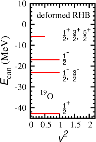
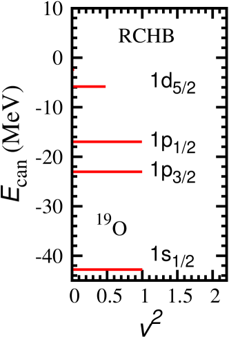
Figure 24: (Color online) Neutron single particle levels in the canonical basis and their occupation probability $v^{2}$ for ¹⁹O from the DRHBc and RCHB calculations. Taken from Ref. [205].

Using the density functional PK1 [138] and a zero range density dependent pairing force [39, 31], the deformed RHB equations are solved in a spherical Dirac Woods-Saxon basis [65] and the deformed potentials and densities are expanded in terms of the Legendre polynomials $P_{\lambda}(\cos\theta)$ (for details see Refs. [108, 30, 31]). In order to check the accuracy of the DRHBc code with the blocking effect, the spherical nucleus ¹⁹O is investigated and the results of the DRHBc code allowing only the spherical components of the fields, i.e., $\lambda=0$, are compared with those obtained in RCHB theory [39]. It is found that both calculations agree well with each other with high precision [205].

In Fig. 24, the neutron single particle levels in the canonical basis for ¹⁹O is shown in comparison with the RCHB results in order to understand the details and validity of the DRHBc calculation. The length of each level is proportional to the occupation probability. In the RCHB calculation, the blocked orbital is 1$d_{5/2}$. In the DRHBc code, a spherical solution is enforced by allowing only $\lambda=0$ component in the Legendre expansion mentioned earlier and therefore the three sublevels of the 1$d_{5/2}$ orbital with $\Omega^{\pi}={1}/{2}^{+}$, ${3}/{2}^{+}$, and ${5}/{2}^{+}$ are degenerate. The present results in Fig. 24 are obtained with the level $\Omega^{\pi}={1}/{2}^{+}$ blocked in the DRHBc code, but blocking any of these three levels gives the same results. From Fig. 24 one finds nice agreement between the results from the DRHBc and RCHB calculations.

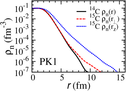
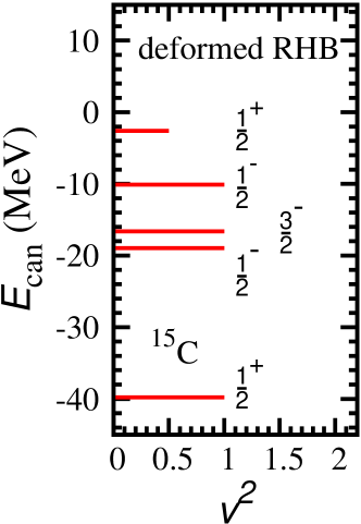
Figure 25: (Color online) (a) Neutron density profiles of ¹⁴C and ¹⁵C in DRHBc calculations with the parameter set PK1. (b) Neutron single particle levels in the canonical basis and their occupation probability $v^{2}$ for ¹⁵C in DRHBc calculation. Taken from Ref. [205].

An application of the DRHBc theory for an exotic and deformed nucleus with an odd number of particles is given in Ref. [205] for the deformed halo candidate nucleus ¹⁵C [233] with the parameter set PK1 [138]. In contrary to the spherical even-even nucleus ¹⁴C, the DRHBc theory predicts a deformation $\beta=0.25$ for the odd-$A$ nucleus ¹⁵C. The neutron root mean square radii of ¹⁴C and ¹⁵C are $2.56$ fm and $2.79$ fm, respectively.

The DRHBc calculations for ¹⁵C lead to a deformed density distribution with an axial symmetry. In Fig. 25, the neutron densities along the symmetry axis $\rho_{n}(r_{z},r_{\perp}=0)$ and perpendicular to the symmetry axis $\rho_{n}(r_{z}=0,r_{\perp})$ are plotted as dashed and dashed-dotted lines. The spherical density for ¹⁴C is also included as a reference by a solid line. It is interesting to see that, in the direction perpendicular to the symmetry axis, the neutron densities are almost the same for ¹⁴C and ¹⁵C at least when $r_{\perp}<6$ fm. Along the symmetry axis the neutron density of ¹⁵C extends much further than that of ¹⁴C. This is partly due to that ¹⁵C is prolate and the weakly bound ${1}/{2}^{+}$ level is occupied.

The single particle levels of ¹⁵C in the canonical basis are plotted in Fig. 25. Since it is a deformed nucleus, the $1p_{3/2}$ orbital is split into two levels with $\Omega^{\pi}={1}/{2}^{-}$ and $\Omega^{\pi}={3}/{2}^{-}$, respectively. There is one neutron occupying in $\Omega^{\pi}={1}/{2}^{+}$ level near the threshold. The occupation probability $v^{2}=0.5$, indicating that it is averaged over the two configurations with $\Omega^{\pi}=\pm{1}/{2}^{+}$. Because of the deformation, this level is a mixture of the spherical orbitals $1d_{5/2}$ ($62\%$) and $2s_{1/2}$ ($36\%$). The weakly-bound feature and the relatively large $s$-wave component of this level results in that the neutron density of ¹⁵C extends further along the symmetry axis.

After the comparison between the DRHBc and the spherical RCHB results for ¹⁹O as well as the application for the deformed neutron-rich nucleus ¹⁵C, the DRHBc with blocking effect proved to be a powerful tool for the study of the odd-$A$ or odd-odd exotic nuclei.

In the development of the DRHBc with the density-dependent meson-nucleon couplings [109], the challenge is the treatment of the density-dependent couplings, meson fields, and potentials in axially deformed system with partial wave method.

In Fig. 26, by taking the $\sigma$ meson as an example, the partial waves of density-dependent coupling strengths $g_{\sigma,\lambda}(r)$ for ³⁸Mg are shown with $g_{\sigma}(\rho_{v})=\sum_{\lambda}g_{\sigma,\lambda}(r)P_{\lambda}(\cos\theta)$. It can be seen that the major component is that with $\lambda=0$, which is more than one order of magnitude larger than the others. The amplitudes of $g_{\sigma,\lambda}$ decrease quickly with increasing $\lambda$ and become negligible when $\lambda\geq 8$. This means that a cutoff $\lambda_{g,\rm{max}}=10$ is enough to provide accurate results.

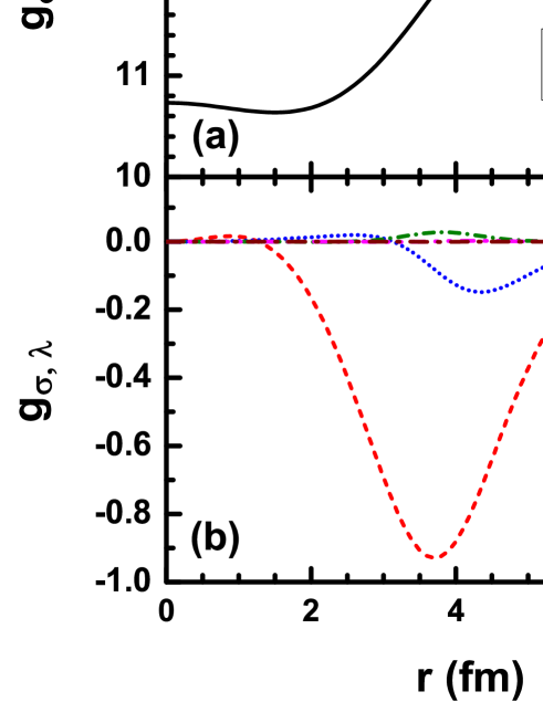
Figure 26: (Color online) Decompositions of coupling strength $g_{\sigma,\lambda}$ with $\lambda=0$ (a) and $\lambda=2,4,6,8,10$ (b) for ³⁸Mg calculated with density-dependent DRHBc theory. Taken from Ref. [109].

By comparing the calculated bulk and single particle properties of neutron-rich nucleus ³⁸Mg in spherical case with $\lambda_{\rho,\rm{max}}=0$ with those obtained by RCHB [39], the density-dependent DRHBc theory is verified [109]. It therefore opens the door to investigate the deformed exotic nuclei with effective density-dependent interactions.

7 Summary and perspectives

In this Topical Review, we have reviewed the progresses on the covariant density functional theory in continuum for the neutron halo phenomenon in both spherical and deformed nuclei.

In the mean field study of nuclear halos, a proper description of nuclear pairing and the continuum contribution is very important. To include properly the contribution of continuum states, the Bogoliubov transformation has been justified to be very useful. The relativistic continuum Hartree-Bogoliubov (RCHB) theory has been developed in which the coupled differential equations are solved in coordinate ($r$) space and the mean field effects of the coupling to the continuum can be fully taken into account.

From the RCHB theory, a self-consistent description of the neutron halo in ¹¹Li has been achieved. The calculated density distribution agrees well with the experiment. It has further been shown that the halo in ¹¹Li is formed by Cooper-pairs scattered in the two levels $1p_{1/2}$ and $2s_{1/2}$ with the former below the Fermi surface and the latter in the continuum. In the RCHB theory, a halo appears if there are several single particle valence orbitals with small orbital angular momenta and correspondingly small centrifugal barriers close to the continuum limit.

For medium and heavy nuclei, the RCHB theory has treated the influence of pairing correlations and many-body effects properly and predicted the existence of more neutrons in the halo. Giant neutron halos, consisting of up to six halo neutrons, have been predicted in Zr and Ca isotopes close to the neutron drip line. When approaching the neutron drip line, the two-neutron separation energies for several nuclei in Ca and Zr isotopes are extremely close to zero, which means that the valence neutrons gradually occupy the loosely bound states and the continuum.

The phenomena of halo and giant halo of neutron-rich even-Ca isotopes were investigated and compared in the framework of the RCHB and non-relativistic Skyrme HFB calculations. It has been found that although halo phenomena exist for Ca isotopes near neutron drip line in both calculations, the halo in the Skyrme HFB calculations starts at a more neutron-rich nucleus than that in the RCHB calculations, and the RCHB calculations have larger neutron root-mean-square radii systematically in $N\geq 40$ than the Skyrme HFB calculations. The former difference comes from the difference in shell structure. The reasons for the latter can be partly explained by the neutron $3s_{1/2}$ orbital, which causes more than $50\%$ of the difference for neutron radii at ⁶⁶Ca.

The relativistic Hartree-Fock-Bogoliubov theory in continuum (RHFBc theory) with density-dependent meson-nucleon couplings has been developed. With this theory, the influence of exchange terms on the formation of neutron halos has been studied. Giant halos as well as ordinary ones were found in Ce isotopes close to the neutron drip line. It was demostrated that the shell structure evolution, when approaching the drip line, is important for the appearance of neutron halos.

The RCHB theory has also been extended to including hyperons and even Ca isotopes ranging from the proton drip line to the neutron drip line have been studied systematically. Compared with ordinary nuclei, the additional one or two $\Lambda$-hyperons lower the Fermi level and the last bound hypernuclei have two more neutrons than the corresponding ordinary nuclei. Giant halo phenomena due to the pairing correlation and the contribution from the continuum have been predicted in Ca hypernuclei, similar to those appearing in ordinary Ca isotopes.

A deformed relativistic Hartree-Bogoliubov theory in continuum (DRHBc theory) has been developed aiming at a proper description of exotic nuclei, particularly those with a large spatial extension. In order to give an adequate consideration of both the contribution of the continuum and the large spatial distribution in exotic nuclei, the deformed RHB equations were solved in a Woods-Saxon (WS) basis in which the radial wave functions have a proper asymptotic behavior at large distance from the nuclear center.

Halo phenomena in deformed nuclei were investigated within the DRHBc theory. These weakly bound quantum systems present interesting examples for the study of the interdependence between the deformation of the core and the particles in the halo. The Mg and Ne isotopes have been studied in details. It was found that in ^42,44Mg, there appears a decoupling of the halo orbitals from the deformation of the core: The core is prolate, but the halo has a slightly oblate shape. The generic conditions for the occurrence of this decoupling effects have been given: the existence and the deformation of a possible neutron halo depends essentially on the quantum numbers of the main components of the single particle orbitals in the vicinity of the Fermi surface.

Definitely there exist lots of open questions on the study of nuclear halos with the covariant density functional theory. We list several of them below.

In the RCHB, RHFBc and DRHBc theories, the box boundary condition has been applied and the continuum is discretized. Therefore one cannot get the width for resonances. With the Green’s function method, the correct asymptotic behavior can be given on the wave function for the continuum states. The Green’s function method has been implemented in the non-relativistic HFB theory [55]. The effort to implement the Green’s function approach in the RHB theory is undertaken and promising preliminary results have been obtained [58].

In the systematic study of giant halos in severl isotope chains, it has been found that the appearance of giant halos and the contribution of continuum are very important in determining the boundary of nuclear chart. Furthermore, the deformation effects will also influence very much the position of drip lines. More systematic study is now carried out to reveal the global impact of the continuum and deformation effects on the nuclear boundary.

If the core and the halo of a nucleus have different shapes, many interesting questions arise: For example, What will happen when the nucleus rotates? What role could the shape fluctuation play? To answer these questions, future works are welcome to implement the angular momentum projection in the DRHBc theory and to use the generator coordinate method (GCM) or to solve Bohr Hamiltonian based on the potential energy surface obtained from constraint DRHBc calculations.

The possible experimental signals of shape decoupling in deformed halo nuclei are certainly interesting topics. The halo feature is connected with relatively large cross sections and narrow longitudinal momentum distributions in knockout reactions. The decoupling between the deformations of the core and the halo may manifest itself by some new experimental observables, e.g., the double-hump shape of longitudinal momentum distribution in single particle removal reactions and new dipole modes, etc. In particular, a combination of the experimental method proposed in Ref. [234] and the theoretical approach developed in Ref. [235] would be useful in the study of longitudinal momentum distribution in single particle removal reactions with deformed halo nuclei as projectiles. The shape decoupling effects may also has some influence on the sub-barrier capture process in heavy ion collisions [236].

References

References

- [1] Thoennessen M 2013 Rep. Prog. Phys. 76 056301–14 see also http://www.nscl.msu.edu/~thoennes/isotopes/ URL http://stacks.iop.org/0034-4885/76/i=5/a=056301
- [2] Erler J, Birge N, Kortelainen M, Nazarewicz W, Olsen E, Perhac A M and Stoitsov M 2012 Nature 486 509–512 URL http://dx.doi.org/10.1038/nature11188
- [3] Afanasjev A, Agbemava S, Ray D and Ring P 2013 Phys. Lett. B 726 680–684 URL http://www.sciencedirect.com/science/article/pii/S037026931300734X
- [4] Agbemava S E, Afanasjev A V, Ray D and Ring P 2014 Phys. Rev. C 89 054320–37 URL http://dx.doi.org/10.1103/PhysRevC.89.054320
- [5] Qu X, Chen Y, Zhang S, Zhao P, Shin I, Lim Y, Kim Y and Meng J 2013 Sci. China-Phys. Mech. Astron. 56 2031–2036 URL http://dx.doi.org/10.1007/s11433-013-5329-5
- [6] Motobayashi T 2010 Nucl. Phys. A 834 707c–712c URL http://dx.doi.org/10.1016/j.nuclphysa.2010.01.128
- [7] Sturm C, Sharkov B and Stöcker H 2010 Nucl. Phys. A 834 682c–687c URL http://dx.doi.org/10.1016/j.nuclphysa.2010.01.124
- [8] Gales S 2010 Nucl. Phys. A 834 717c–723c URL http://dx.doi.org/10.1016/j.nuclphysa.2010.01.130
- [9] Thoennessen M 2010 Nucl. Phys. A 834 688c–693c URL http://dx.doi.org/10.1016/j.nuclphysa.2010.01.125
- [10] Choi S KoRIA project - RI accelerator in Korea invited talk given in International Symposium on Nuclear Physics in Asia, 14-15 October, 2010, Beihang University, Beijing URL http://indico.ihep.ac.cn/conferenceTimeTable.py?confId=1714
- [11] Xia J W, Zhan W L, Wei B W, Yuan Y J, Song M T, Zhang W Z, Yang X D, Yuan P, Gao D Q, Zhao H W, Yang X T, Xiao G Q, Man K T, Dang J R, Cai X H, Wang Y F, Tang J Y, Qiao W M, Rao Y N, He Y, Mao L Z and Zhou Z Z 2002 Nucl. Instrum. Methods Phys. Res. A 488 11–25 URL http://dx.doi.org/10.1016/S0168-9002(02)00475-8
- [12] Zhan W, Xu H, Xiao G, Xia J, Zhao H and Yuan Y 2010 Nucl. Phys. A 834 694c–700c URL http://dx.doi.org/10.1016/j.nuclphysa.2010.01.126
- [13] Müller A C and Sherrill B M 1993 Annu. Rev. Nucl. Part. Sci. 43 529–583 URL http://dx.doi.org/10.1146/annurev.ns.43.120193.002525
- [14] Tanihata I 1995 Prog. Part. Nucl. Phys. 35 505–573 URL http://dx.doi.org/10.1016/0146-6410(95)00046-L
- [15] Hansen P G, Jensen A S and Jonson B 1995 Annu. Rev. Nucl. Part. Sci. 45 591–634 URL http://dx.doi.org/10.1146/annurev.ns.45.120195.003111
- [16] Casten R F and Sherrill B M 2000 Prog. Part. Nucl. Phys. 45 S171–S223 URL http://dx.doi.org/10.1016/S0146-6410(00)90013-9
- [17] Bertulani C A, Hussein M S and Münzenberg G 2001 Physics of Radioactive Beams (Nova Science Publishers, Inc., Huntington, New York) URL http://books.google.com/books?id=sxWMQAAACAAJ
- [18] Johnson B 2004 Phys. Rep. 389 1–59 URL http://dx.doi.org/10.1016/j.physrep.2003.07.004
- [19] Jensen A S, Riisager K, Fedorov D V and Garrido E 2004 Rev. Mod. Phys. 76 215–261 URL http://link.aps.org/abstract/RMP/v76/p215
- [20] Meng J, Toki H, Zhou S G, Zhang S Q, Long W H and Geng L S 2006 Prog. Part. Nucl. Phys. 57 470–563 URL http://dx.doi.org/10.1016/j.ppnp.2005.06.001
- [21] Ershov S N, Grigorenko L V, Vaagen J S and Zhukov M V 2010 J. Phys. G: Nucl. Phys. 37 064026–15 URL http://stacks.iop.org/0954-3899/37/i=6/a=064026
- [22] Frederico T, Delfino A, Tomio L and Yamashita M T 2012 Prog. Part. Nucl. Phys. 67 939–994 URL http://www.sciencedirect.com/science/article/pii/S0146641012000907
- [23] Riisager K 2013 Phys. Scr. T152 014001–13 URL http://dx.doi.org/10.1088/0031-8949/2013/T152/014001
- [24] Tanihata I, Hamagaki H, Hashimoto O, Shida Y, Yoshikawa N, Sugimoto K, Yamakawa O, Kobayashi T and Takahashi N 1985 Phys. Rev. Lett. 55 2676–2679 URL http://link.aps.org/abstract/PRL/v55/p2676
- [25] Ozawa A, Kobayashi T, Suzuki T, Yoshida K and Tanihata I 2000 Phys. Rev. Lett. 84 5493–5495 URL http://link.aps.org/doi/10.1103/PhysRevLett.84.5493
- [26] Warburton E K, Becker J A and Brown B A 1990 Phys. Rev. C 41 1147–1166 URL http://link.aps.org/doi/10.1103/PhysRevC.41.1147
- [27] Adrich P, Klimkiewicz A, Fallot M, Boretzky K, Aumann T, Cortina-Gil D, Pramanik U D, Elze T W, Emling H, Geissel H, Hellstrom M, Jones K L, Kratz J V, Kulessa R, Leifels Y, Nociforo C, Palit R, Simon H, Surowka G, Summerer K and Walus W 2005 Phys. Rev. Lett. 95 132501–4 URL http://link.aps.org/abstract/PRL/v95/e132501
- [28] Meng J and Ring P 1998 Phys. Rev. Lett. 80 460–463 URL http://link.aps.org/abstract/PRL/v80/p460
- [29] Meng J, Toki H, Zeng J Y, Zhang S Q and Zhou S G 2002 Phys. Rev. C 65 041302(R)–4 URL http://link.aps.org/abstract/PRC/v65/e041302
- [30] Zhou S G, Meng J, Ring P and Zhao E G 2010 Phys. Rev. C 82 011301(R)–5 URL http://link.aps.org/doi/10.1103/PhysRevC.82.011301
- [31] Li L, Meng J, Ring P, Zhao E G and Zhou S G 2012 Phys. Rev. C 85 024312–17 URL http://link.aps.org/doi/10.1103/PhysRevC.85.024312
- [32] Dobaczewski J, Michel N, Nazarewicz W, Ploszajczak M and Rotureau J 2007 Prog. Part. Nucl. Phys. 59 432–445 URL http://dx.doi.org/10.1016/j.ppnp.2007.01.022
- [33] Bertsch G F and Esbensen H 1991 Annals of Physics 209 327–363 URL http://dx.doi.org/10.1016/0003-4916(91)90033-5
- [34] Meng J and Ring P 1996 Phys. Rev. Lett. 77 3963–3966 URL http://link.aps.org/abstract/PRL/v77/p3963
- [35] Meng J 1998 Phys. Rev. C 57 1229–1232 URL http://dx.doi.org/10.1103/PhysRevC.57.1229
- [36] Bulgac A 1980 Hartree-Fock-Bogoliubov approximation for finite systems IPNE FT-194-1980, Bucharest (arXiv: nucl-th/9907088) URL http://arxiv.org/abs/nucl-th/9907088
- [37] Dobaczewski J, Flocard H and Treiner J 1984 Nucl. Phys. A 422 103–139 URL http://dx.doi.org/10.1016/0375-9474(84)90433-0
- [38] Pöschl W, Vretenar D, Lalazissis G A and Ring P 1997 Phys. Rev. Lett. 79 3841–3844 URL http://link.aps.org/abstract/PRL/v79/p3841
- [39] Meng J 1998 Nucl. Phys. A 635 3–42 URL http://dx.doi.org/10.1016/S0375-9474(98)00178-X
- [40] Yang S C, Meng J and Zhou S G 2001 Chin. Phys. Lett. 18 196–198 URL http://stacks.iop.org/0256-307X/18/196
- [41] Cao L G and Ma Z Y 2002 Phys. Rev. C 66 024311–5 URL http://link.aps.org/doi/10.1103/PhysRevC.66.024311
- [42] Zhang S S, Meng J, Zhou S G and Hillhouse G C 2004 Phys. Rev. C 70 034308–8 (Preprint nucl-th/0403013) URL http://link.aps.org/abstract/PRC/v70/e034308
- [43] Zhang L, Zhou S G, Meng J and Zhao E G 2008 Phys. Rev. C 77 014312–6 (Preprint 0712.3087) URL http://link.aps.org/doi/10.1103/PhysRevC.77.014312
- [44] Zhou S G, Meng J and Zhao E G 2009 J. Phys. B: At. Mol. Phys. 42 245001–5 (Preprint 0911.1171) URL http://dx.doi.org/10.1088/0953-4075/42/24/245001
- [45] Li Z P, Meng J, Zhang Y, Zhou S G and Savushkin L N 2010 Phys. Rev. C 81 034311–6 URL http://link.aps.org/doi/10.1103/PhysRevC.81.034311
- [46] Guo J Y, Fang X Z, Jiao P, Wang J and Yao B M 2010 Phys. Rev. C 82 034318–8 URL http://link.aps.org/doi/10.1103/PhysRevC.82.034318
- [47] Sandulescu N, Van Giai N and Liotta R J 2000 Phys. Rev. C 61 061301(R)–5 URL http://link.aps.org/abstract/PRC/v61/e061301
- [48] Sandulescu N, Geng L S, Toki H and Hillhouse G C 2003 Phys. Rev. C 68 054323–6 URL http://link.aps.org/doi/10.1103/PhysRevC.68.054323
- [49] Zhang S S, Zhao E G and Zhou S G 2013 Euro. Phys. J. A 49 77 (Preprint 1105.0504) URL http://dx.doi.org/10.1140/epja/i2013-13077-8
- [50] Zhang S S, Smith M S, Kang Z S and Zhao J 2014 Phys. Lett. B 730 30–35 URL http://www.sciencedirect.com/science/article/pii/S0370269314000355
- [51] Belyaev S T, Smirnov A V, Tolokonnikov S V and Fayans S A 1987 Sov. J. Nucl. Phys. 45 783
- [52] Shlomo S and Bertsch G 1975 Nucl. Phys. A 243 507–518 URL http://dx.doi.org/10.1016/0375-9474(75)90292-4
- [53] Matsuo M 2001 Nucl. Phys. A 696 371–395 URL http://dx.doi.org/10.1016/S0375-9474(01)01133-2
- [54] Oba H and Matsuo M 2009 Phys. Rev. C 80 024301–14 URL http://link.aps.org/doi/10.1103/PhysRevC.80.024301
- [55] Zhang Y, Matsuo M and Meng J 2011 Phys. Rev. C 83 054301–11 URL http://link.aps.org/doi/10.1103/PhysRevC.83.054301
- [56] Zhang Y, Matsuo M and Meng J 2012 Phys. Rev. C 86 054318–12 URL http://link.aps.org/doi/10.1103/PhysRevC.86.054318
- [57] Zhang Y, Matsuo M and Meng J 2014 Phys. Rev. C 90 034313–5 URL http://dx.doi.org/10.1103/PhysRevC.90.034313
- [58] Sun T T, Zhang S Q, Zhang Y, Hu J N and Meng J 2014 Phys. Rev. C 90(5) 054321 URL http://link.aps.org/doi/10.1103/PhysRevC.90.054321
- [59] Vautherin D and Brink D M 1972 Phys. Rev. C 5 626–647 URL http://link.aps.org/abstract/PRC/v5/p626
- [60] Decharge J and Gogny D 1980 Phys. Rev. C 21 1568–1593 URL http://link.aps.org/doi/10.1103/PhysRevC.21.1568
- [61] Gambhir Y K, Ring P and Thimet A 1990 Ann. Phys. (NY) 198 132–179 URL http://dx.doi.org/10.1016/0003-4916(90)90330-Q
- [62] Zhou S G, Meng J, Yamaji S and Yang S C 2000 Chin. Phys. Lett. 17 717–719 URL http://dx.doi.org/10.1088/0256-307X/17/10/006
- [63] Stoitsov M V, Dobaczewski J, Ring P and Pittel S 2000 Phys. Rev. C 61 034311–14 URL http://link.aps.org/abstract/PRC/v61/e034311
- [64] Stoitsov M V, Dobaczewski J, Nazarewicz W, Pittel S and Dean D J 2003 Phys. Rev. C 68 054312–11 URL http://link.aps.org/abstract/PRC/v68/e054312
- [65] Zhou S G, Meng J and Ring P 2003 Phys. Rev. C 68 034323–12 (Preprint nucl-th/0303031) URL http://link.aps.org/abstract/PRC/v68/e034323
- [66] Serot B D and Walecka J D 1986 Adv. Nucl. Phys. 16 1–327
- [67] Ring P 1996 Prog. Part. Nucl. Phys. 37 193–263 URL http://dx.doi.org/10.1016/0146-6410(96)00054-3
- [68] Vretenar D, Afanasjev A V, Lalazissis G A and Ring P 2005 Phys. Rep. 409 101–259 URL http://dx.doi.org/10.1016/j.physrep.2004.10.001
- [69] Nikšić T, Vretenar D and Ring P 2011 Prog. Part. Nucl. Phys. 66 519–548 URL http://dx.doi.org/10.1016/j.ppnp.2011.01.055
- [70] Meng J, Peng J, Zhang S Q and Zhao P W 2013 Frontiers of Physics 8(1) 55–79
- [71] Brockmann R and Machleidt R 1990 Phys. Rev. C 42 1965–1980 URL http://link.aps.org/abstract/PRC/v42/p1965
- [72] Sharma M M, Lalazissis G A and Ring P 1993 Phys. Lett. B 317 9–13 URL http://dx.doi.org/10.1016/0370-2693(93)91561-Z
- [73] Arima A, Harvey M and Shimizu K 1969 Phys. Lett. B 30 517–522 URL http://www.sciencedirect.com/science/article/B6TVN-470W8D8-1VW/1/3dec596cd3ba7d158a639c410a814db7
- [74] Hecht K T and Adler A 1969 Nucl. Phys. A 137 129–143 URL http://www.sciencedirect.com/science/article/B6TVB-47201GS-1D2/1/81a3cea8030569b83b7cce4f6d25d1ee
- [75] Ginocchio J N 1997 Phys. Rev. Lett. 78 436–439 URL http://link.aps.org/abstract/PRL/v78/p436
- [76] Meng J, Sugawara-Tanabe K, Yamaji S, Ring P and Arima A 1998 Phys. Rev. C 58 R628–631 URL http://link.aps.org/abstract/PRC/v58/pR628
- [77] Meng J, Sugawara-Tanabe K, Yamaji S and Arima A 1999 Phys. Rev. C 59 154–163 URL http://link.aps.org/abstract/PRC/v59/p154
- [78] Long W H, Sagawa H, Meng J and Van Giai N 2006 Phys. Lett. B 639 242–247 URL http://dx.doi.org/10.1016/j.physletb.2006.05.065
- [79] Liang H, Zhao P, Zhang Y, Meng J and Giai N V 2011 Phys. Rev. C 83 041301(R)–5 URL http://link.aps.org/doi/10.1103/PhysRevC.83.041301
- [80] Lu B N, Zhao E G and Zhou S G 2012 Phys. Rev. Lett. 109 072501–5 (Preprint 1204.5069) URL http://link.aps.org/doi/10.1103/PhysRevLett.109.072501
- [81] Lu B N, Zhao E G and Zhou S G 2013 Phys. Rev. C 88 024323–11 URL http://link.aps.org/doi/10.1103/PhysRevC.88.024323
- [82] Liang H, Meng J and Zhou S G 2015 Physics Reports 570 1 – 84 URL http://www.sciencedirect.com/science/article/pii/S0370157315000502
- [83] Zhou S G, Meng J and Ring P 2003 Phys. Rev. Lett. 91 262501–4 (Preprint nucl-th/0304067) URL http://link.aps.org/abstract/PRL/v91/e262501
- [84] Liang H, Hui Long W, Meng J and Van Giai N 2010 Eur. Phys. J. A 44 119–124 URL http://dx.doi.org/10.1140/epja/i2010-10938-6
- [85] Koepf W and Ring P 1989 Nucl. Phys. A 493 61–82 URL http://dx.doi.org/10.1016/0375-9474(89)90532-0
- [86] Yao J M, Chen H and Meng J 2006 Phys. Rev. C 74 024307–11 URL http://link.aps.org/doi/10.1103/PhysRevC.74.024307
- [87] Arima A 2011 Sci. China-Phys. Mech. Astron. 54 188–193 URL http://dx.doi.org/10.1007/s11433-010-4224-6
- [88] Li J, Yao J M, Meng J and Arima A 2011 Prog. Theor. Phys. 125 1185–1192 URL http://ptp.ipap.jp/link?PTP/125/1185/
- [89] Wei J, Li J and Meng J 2012 Prog. Theor. Phys. Suppl. 196 400–406 URL http://ptp.ipap.jp/link?PTPS/196/400/
- [90] Afanasjev A V, Ring P and König J 2000 Nucl. Phys. A 676 196–244 URL http://www.sciencedirect.com/science/article/pii/S0375947400001871
- [91] Zhao P W, Peng J, Liang H Z, Ring P and Meng J 2012 Phys. Rev. C 85 054310–14 URL http://link.aps.org/doi/10.1103/PhysRevC.85.054310
- [92] Zhao P W, Peng J, Liang H Z, Ring P and Meng J 2011 Phys. Rev. Lett. 107 122501–5 URL http://link.aps.org/doi/10.1103/PhysRevLett.107.122501
- [93] Zhao P W, Zhang S Q, Peng J, Liang H Z, Ring P and Meng J 2011 Phys. Lett. B 699 181–186 URL http://dx.doi.org/10.1016/j.physletb.2011.03.068
- [94] Koepf W, Gambhir Y K, Ring P and Sharma M M 1991 Z. Phys. A 340 119–124 URL http://dx.doi.org/10.1007/BF01303823
- [95] Sharma M M, Lalazissis G A, Hillebrandt W and Ring P 1994 Phys. Rev. Lett. 72 1431–1434 URL http://link.aps.org/doi/10.1103/PhysRevLett.72.1431
- [96] Zhu Z Y, Shen W Q, Cai Y H and Ma Y G 1994 Phys. Lett. B 328 1–4 URL http://dx.doi.org/10.1016/0370-2693(94)90418-9
- [97] Ren Z, Mittig W, Chen B and Ma Z 1995 Phys. Rev. C 52 R20–R22 URL http://link.aps.org/doi/10.1103/PhysRevC.52.R20
- [98] Ren Z, Xu G, Chen B, Ma Z and Mittig W 1995 Phys. Lett. B 351 11–17 URL http://dx.doi.org/10.1016/0370-2693(95)00364-Q
- [99] Ren Z, Chen B, Ma Z and Xu G 1996 Phys. Rev. C 53 R572–575 URL http://link.aps.org/abstract/PRC/v53/pR572
- [100] Ren Z Z, Faessler A and Bobyk A 1998 Phys. Rev. C 57 2752–2755 URL http://link.aps.org/doi/10.1103/PhysRevC.57.2752
- [101] Meng J, Tanihata I and Yamaji S 1998 Phys. Lett. B 419 1–6 URL http://www.sciencedirect.com/science/article/B6TVN-3VGPWM4-44/1/f83ff8aa3662905a3a6f21e8b7464573
- [102] Vretenar D, Poschl W, Lalazissis G A and Ring P 1998 Phys. Rev. C 57 R1060–R1063 URL http://link.aps.org/doi/10.1103/PhysRevC.57.R1060
- [103] Lü H F and Meng J 2002 Chin. Phys. Lett. 19 1775–1778 URL http://stacks.iop.org/0256-307X/19/i=12/a=310
- [104] Lü H F, Meng J, Zhang S Q and Zhou S G 2003 Eur. Phys. J. A 17 19–24 URL http://dx.doi.org/10.1140/epja/i2002-10136-3
- [105] Lu H F, Meng J and Zhang S Q 2003 High Ener. Phys. Nucl. Phys. 27 411–415 (in Chinese)
- [106] Lü H F 2008 Chin. Phys. Lett. 25 3613–3616 URL http://stacks.iop.org/0256-307X/25/i=10/a=025
- [107] Long W H, Ring P, Meng J, Van Giai N and Bertulani C A 2010 Phys. Rev. C 81 031302(R)–5 URL http://dx.doi.org/10.1103/PhysRevC.81.031302
- [108] Zhou S G, Meng J and Ring P 2008 Deformed relativistic Hartree-Bogoliubov model for exotic nuclei Physics of Unstable Nuclei ed Khoa D T, Egelhof P, Gales S, Van Giai N and Motobayashi T (World Scientific) pp 402–408 Proceedings of the International Symposium on Physics of Unstable Nuclei, July 3-7, 2007, Hoi An, Vietnam (Preprint 0803.1376) URL http://dx.doi.org/10.1142/9789812776150_0059
- [109] Chen Y, Li L, Liang H and Meng J 2012 Phys. Rev. C 85 067301–5 URL http://link.aps.org/doi/10.1103/PhysRevC.85.067301
- [110] Afanasjev A, Fossan D, Lane G and Ragnarsson I 1999 Phys. Rep. 322 1–124 URL http://dx.doi.org/10.1016/S0370-1573(99)00035-6
- [111] Ginocchio J N 2005 Phys. Rep. 414 165–261 URL http://dx.doi.org/10.1016/j.physrep.2005.04.003
- [112] Meng J, Peng J, Zhang S Q and Zhao P W 2013 Front. Phys. 8 55–79 URL http://dx.doi.org/10.1007/s11467-013-0287-y
- [113] Long W, Sagawa H, Giai N V and Meng J 2007 Phys. Rev. C 76 034314–11 URL http://link.aps.org/doi/10.1103/PhysRevC.76.034314
- [114] Long W H, Ring P, Giai N V and Meng J 2010 Phys. Rev. C 81 024308–10 URL http://link.aps.org/doi/10.1103/PhysRevC.81.024308
- [115] Nikolaus B A, Hoch T and Madland D G 1992 Phys. Rev. C 46 1757–1781 URL http://link.aps.org/doi/10.1103/PhysRevC.46.1757
- [116] Burvenich T, Madland D G, Maruhn J A and Reinhard P G 2002 Phys. Rev. C 65 044308–23 URL http://link.aps.org/doi/10.1103/PhysRevC.65.044308
- [117] Nikšić T, Vretenar D and Ring P 2008 Phys. Rev. C 78 034318–19 URL http://link.aps.org/doi/10.1103/PhysRevC.78.034318
- [118] Zhao P W, Li Z P, Yao J M and Meng J 2010 Phys. Rev. C 82 054319–14 URL http://link.aps.org/doi/10.1103/PhysRevC.82.054319
- [119] Friar J, Madland D and Lynn B 1996 Phys. Rev. C 53 3085–3087 URL http://dx.doi.org/10.1103/PhysRevC.53.3085
- [120] Manohar A and Georgi H 1984 Nucl. Phys. B 234 189–212 URL http://dx.doi.org/10.1016/0550-3213(84)90231-1
- [121] Liang H, Zhao P, Ring P, Roca-Maza X and Meng J 2012 Phys. Rev. C 86 021302–5 URL http://link.aps.org/doi/10.1103/PhysRevC.86.021302
- [122] Sulaksono A, Bürvenich T, Maruhn J A, Reinhard P G and Greiner W 2003 Annals of Physics 308 354–370 URL http://dx.doi.org/10.1016/S0003-4916(03)00146-5
- [123] Kucharek H and Ring P 1991 Z. Phys. A 339 23–35 URL http://dx.doi.org/10.1007/BF01282930
- [124] Berger J F, Girod M and Gogny D 1984 Nucl. Phys. A 428 23–36 URL http://dx.doi.org/10.1016/0375-9474(84)90240-9
- [125] Meng J 1998 Nucl. Phys. A 635 3–42
- [126] Bouyssy A, Mathiot J F, Van Giai N and Marcos S 1987 Phys. Rev. C 36 380–401 URL http://link.aps.org/doi/10.1103/PhysRevC.36.380
- [127] Long W H, Van Giai N and Meng J 2006 Phys. Lett. B 640 150–154 URL http://dx.doi.org/10.1016/j.physletb.2006.07.064
- [128] Koepf W and Ring P 1991 Z. Phys. A 339 81–90 URL http://dx.doi.org/10.1007/BF01282936
- [129] Terasaki J, Heenen P H, Flocard H and Bonche P 1996 Nucl. Phys. A 600 371–386 URL http://dx.doi.org/10.1016/0375-9474(96)00036-X
- [130] Teran E, Oberacker V E and Umar A S 2003 Phys. Rev. C 67 064314–13 URL http://link.aps.org/abstract/PRC/v67/e064314
- [131] Tajima N 2004 Phys. Rev. C 69 034305–22 URL http://link.aps.org/abstract/PRC/v69/e034305
- [132] Stoitsov M, Michel N and Matsuyanagi K 2008 Phys. Rev. C 77 054301–12 URL http://link.aps.org/abstract/PRC/v77/e054301
- [133] Nakada H 2008 Nucl. Phys. A 808 47–59 URL http://www.sciencedirect.com/science/article/B6TVB-4SMNXRD-1/2/5b3d912dab1e2b213bc161417b54afd3
- [134] Schunck N and Egido J L 2008 Phys. Rev. C 78 064305–14 URL http://link.aps.org/abstract/PRC/v78/e064305
- [135] Zhou S G, Meng J and Ring P 2006 AIP Conf. Proc. 865 90–95 URL http://link.aip.org/link/?APC/865/90/1
- [136] Price C E and Walker G E 1987 Phys. Rev. C 36 354–364 URL http://link.aps.org/abstract/PRC/v36/p354
- [137] Bonche P, Flocard H, Heenen P H, Krieger S J and Weiss M S 1985 Nucl. Phys. A 443 39–63 URL http://dx.doi.org/10.1016/0375-9474(85)90320-3
- [138] Long W, Meng J, Giai N V and Zhou S G 2004 Phys. Rev. C 69 034319–15 (Preprint nucl-th/0311031) URL http://link.aps.org/abstract/PRC/v69/e034319
- [139] Zhao P W, Sun B Y and Meng J 2009 Chin. Phys. Lett. 26 112102–3 URL http://stacks.iop.org/0256-307X/26/i=11/a=112102
- [140] Meng J, Lü H F, Zhang S Q and Zhou S G 2003 Nucl. Phys. A 722 366c–371c URL http://dx.doi.org/10.1016/S0375-9474(03)01391-5
- [141] Meng J, Pöschl W and Ring P 1997 Z. Phys. A 358 123–124 0939-7922 URL http://dx.doi.org/10.1007/s002180050285
- [142] Meng J and Tanihata I 1999 Nucl. Phys. A 650 176–196 URL http://www.sciencedirect.com/science/article/B6TVB-3WSV1PV-3/1/a568ac0e55bc594c2a148681ea97c9e4
- [143] Meng J, Zhou S G and Tanihata I 2002 Phys. Lett. B 532 209–214 (Preprint nucl-th/0107039) URL http://dx.doi.org/10.1016/S0370-2693(02)01574-5
- [144] Zhang S Q, Meng J, Zhou S G and Zeng J Y 2002 Chin. Phys. Lett. 19 312–314 URL http://dx.doi.org/10.1088/0256-307X/19/3/308
- [145] Zhang S Q, Meng J and Zhou S G 2003 Sci. China G 46 632–658 (Preprint nucl-th/0302032) URL http://www.scichina.com:8083/sciGe/EN/abstract/abstract408047.shtml
- [146] Bertsch G F, Brown B A and Sagawa H 1989 Phys. Rev. C 39 1154–1157 URL http://link.aps.org/doi/10.1103/PhysRevC.39.1154
- [147] Sagawa H 1992 Physics Letters B 286 7–12 URL http://dx.doi.org/10.1016/0370-2693(92)90150-3
- [148] Rotival V and Duguet T 2009 Phys. Rev. C 79 054308–24 URL http://link.aps.org/abstract/PRC/v79/e054308
- [149] Rotival V, Bennaceur K and Duguet T 2009 Phys. Rev. C 79 054309–21 URL http://link.aps.org/abstract/PRC/v79/e054309
- [150] Meng J, Tanihata I and Yamaji S 1998 Phys. Lett. B 419 1–6
- [151] Im S and Meng J 2000 Phys. Rev. C 61 047302–4 URL http://link.aps.org/doi/10.1103/PhysRevC.61.047302
- [152] Mizutori S, Dobaczewski J, Lalazissis G A, Nazarewicz W and Reinhard P G 2000 Phys. Rev. C 61 044326–14 URL http://link.aps.org/abstract/PRC/v61/e044326
- [153] Sharma M M, Nagarajan M A and Ring P 1993 Phys. Lett. B 312 377–381 URL http://www.sciencedirect.com/science/article/B6TVN-470G13S-69/2/b3e2b625f3a9be50fc271b3986c87fda
- [154] Zhao P W, Song L S, Sun B, Geissel H and Meng J 2012 Phys. Rev. C 86 064324–6 URL http://link.aps.org/doi/10.1103/PhysRevC.86.064324
- [155] Sun B, Zhao P and Meng J 2011 Sci. China-Phys. Mech. Astron. 54 210–214 URL http://dx.doi.org/10.1007/s11433-010-4222-8
- [156] Lu B N, Zhao E G and Zhou S G 2012 Phys. Rev. C 85 011301(R)–5 URL http://link.aps.org/doi/10.1103/PhysRevC.85.011301
- [157] Lu B N, Zhao J, Zhao E G and Zhou S G 2014 Phys. Rev. C 89 014323–15 URL http://link.aps.org/doi/10.1103/PhysRevC.89.014323
- [158] Lalazissis G A, Vretenar D, P?schl W and Ring P 1998 Nucl. Phys. A 632 363–382 URL http://www.sciencedirect.com/science/article/B6TVB-3T0XR5K-3/2/719c3043312d1ae0173bf408684416a5
- [159] Bennaceur K, Dobaczewski J and Ploszajczak M 2000 Phys. Lett. B 496 154–160 URL http://www.sciencedirect.com/science/article/B6TVN-41XM9PX-4/2/d261a458d12e29f0df079cabe8081520
- [160] Dobaczewski J, Nazarewicz W and Reinhard P G 2001 Nucl. Phys. A 693 361–373 URL http://dx.doi.org/10.1016/S0375-9474(01)00993-9
- [161] Terasaki J, Zhang S Q, Zhou S G and Meng J 2006 Phys. Rev. C 74 054318–6 (Preprint nucl-th/0603005) URL http://link.aps.org/abstract/PRC/v74/e054318
- [162] Terasaki J, Zhang S Q, Zhou S G and Meng J 2006 Int. J. Mod. Phys. E 15 1833–1841 URL http://www.worldscinet.com/cgi-bin/details.cgi?id=pii:S0218301306005010&type=html
- [163] Grasso M, Yoshida S, Sandulescu N and Van Giai N 2006 Phys. Rev. C 74 064317–7 URL http://link.aps.org/abstract/PRC/v74/e064317
- [164] Grasso M, Sandulescu N, Van Giai N and Liotta R J 2001 Phys. Rev. C 64 064321–9 URL http://link.aps.org/abstract/PRC/v64/e064321
- [165] Boguta J and Bodmer A R 1977 Nucl. Phys. A 292 413–428
- [166] Brockmann R and Weise W 1977 Phys. Lett. B 69 167–169 URL http://dx.doi.org/10.1016/0370-2693(77)90635-9
- [167] Horowitz C J and Serot B D 1984 Phys. Lett. B 140 181–186 URL http://dx.doi.org/10.1016/0370-2693(84)90916-X
- [168] Bielajew A F and Serot B D 1984 Annals of Physics 156 215–264 URL http://dx.doi.org/10.1016/0003-4916(84)90034-4
- [169] Bouyssy A, Marcos S, Mathiot J and Van Giai N 1985 Physical Review Letters 55 1731–1733 URL http://dx.doi.org/10.1103/PhysRevLett.55.1731
- [170] Blunden P G and Iqbal M J 1987 Phys. Lett. B 196 295–298 URL http://dx.doi.org/10.1016/0370-2693(87)90734-9
- [171] Bernardos P, Fomenko V, Giai N, Quelle M, Marcos S, Niembro R and Savushkin L 1993 Phys. Rev. C 48 2665–2672 URL http://dx.doi.org/10.1103/PhysRevC.48.2665
- [172] Marcos S, Savushkin L N, Fomenko V N, Löpez-Quelle M and Niembro R 2004 J. Phys. G 30 703–721 URL http://dx.doi.org/10.1088/0954-3899/30/6/002
- [173] Long W H, Sagawa H, Meng J and Van Giai N 2008 Europhys. Lett. 82 12001 URL http://dx.doi.org/doi/10.1209/0295-5075/82/12001
- [174] Liang H, Van Giai N and Meng J 2008 Phys. Rev. Lett. 101 122502–4 URL http://link.aps.org/doi/10.1103/PhysRevLett.101.122502
- [175] Sun B Y, Long W H, Meng J and Lombardo U 2008 Phys. Rev. C 78 065805–14 URL http://link.aps.org/doi/10.1103/PhysRevC.78.065805
- [176] Liang H, Giai N V and Meng J 2009 Phys. Rev. C 79 064316–7 URL http://link.aps.org/doi/10.1103/PhysRevC.79.064316
- [177] Liang H, Zhao P and Meng J 2012 Phys. Rev. C 85(6) 064302 URL http://link.aps.org/doi/10.1103/PhysRevC.85.064302
- [178] Jaminon M and Mahaux C 1989 Phys. Rev. C 40 354–367 URL http://dx.doi.org/10.1103/PhysRevC.40.354
- [179] Tarpanov D, Liang H, Van Giai N and Stoyanov C 2008 Phys. Rev. C 77 054316 (pages 5) URL http://link.aps.org/abstract/PRC/v77/e054316
- [180] Long W H, Nakatsukasa T, Sagawa H, Meng J, Nakada H and Zhang Y 2009 Phys. Lett. B 680 428–431 URL http://dx.doi.org/10.1016/j.physletb.2009.09.034
- [181] Moreno-Torres M, Grasso M, Liang H, De Donno V, Anguiano M and Van Giai N 2010 Phys. Rev. C 81 064327–13 URL http://dx.doi.org/10.1103/PhysRevC.81.064327
- [182] Lalazissis G A, Nikšić T, Vretenar D and Ring P 2005 Phys. Rev. C 71 024312–10 URL http://link.aps.org/abstract/PRC/v71/e024312
- [183] Audi G, Wapstra A H and Thibault C 2003 Nucl. Phys. A 729 337–676 URL http://dx.doi.org/10.1016/j.nuclphysa.2003.11.003
- [184] Rufa M, Schaffner J, Maruhn J, Stoecker H, Greiner W and Reinhard P G 1990 Phys. Rev. C 42 2469–2478 URL http://link.aps.org/doi/10.1103/PhysRevC.42.2469
- [185] Rufa M, Schaffner J, Maruhn J, Stoecker H, Greiner W and Reinhard P G 1991 Phys. Rev. C 43 2020–2020 (Erratum) URL http://link.aps.org/doi/10.1103/PhysRevC.43.2020
- [186] Liang H, Meng J and Zhou S G 2015 Phys. Rep. 570 1–84 URL http://www.sciencedirect.com/science/article/pii/S0370157315000502
- [187] Wang N, Liu M, Wu X and Meng J 2014 Phys. Lett. B 734 215–219 URL http://www.sciencedirect.com/science/article/pii/S037026931400358X
- [188] Ring P and Schuck P 1980 The nuclear many-body problem (Springer-Verlag, New York)
- [189] Audi G and Wapstra A H 1995 Nucl. Phys. A 595 409–480 URL http://www.sciencedirect.com/science/article/B6TVB-3YYTR61-1/1/4d118297fb99a6b35c8527554b90e57d
- [190] Wang N, Liu M and Wu X 2010 Phys. Rev. C 81 044322– URL http://link.aps.org/doi/10.1103/PhysRevC.81.044322
- [191] Wang N, Liang Z, Liu M and Wu X 2010 Phys. Rev. C 82 044304– URL http://link.aps.org/doi/10.1103/PhysRevC.82.044304
- [192] Liu M, Wang N, Deng Y and Wu X 2011 Phys. Rev. C 84 014333–8 URL http://link.aps.org/doi/10.1103/PhysRevC.84.014333
- [193] Sobiczewski A and Litvinov Y A 2014 Phys. Rev. C 89(2) 024311 URL http://link.aps.org/doi/10.1103/PhysRevC.89.024311
- [194] Sobiczewski A and Litvinov Y A 2014 Phys. Rev. C 90 017302– URL http://link.aps.org/doi/10.1103/PhysRevC.90.017302
- [195] Li Zhu Niu Zhong-Ming S B H W N M J 2012 Acta Physica Sinica 61 72601 (pages 0) URL http://wulixb.iphy.ac.cn/EN/abstract/article_47169.shtml
- [196] Mendoza-Temis J d J, Martinez-Pinedo G, Langanke K, Bauswein A and Janka H T 2014 On the robustness of the r-process in neutron-star mergers arXiv:1409.6135 [astro-ph.HE] (Preprint 1409.6135) URL http://arxiv.org/abs/1409.6135
- [197] Audi G, Wang M, Wapstra A H, Kondev F G, MacCormick M, X X and Pfeiffer B 2012 Chin. Phys. C 36 1287–1602 URL http://amdc.impcas.ac.cn/
- [198] Chen Y, Ring P and Meng J 2014 Phys. Rev. C 89 014312–9 URL http://link.aps.org/doi/10.1103/PhysRevC.89.014312
- [199] Misu T, Nazarewicz W and Åberg S 1997 Nucl. Phys. A 614 44–70 URL http://dx.doi.org/10.1016/S0375-9474(96)00458-7
- [200] Li X and Heenen P H 1996 Phys. Rev. C 54 1617–1621 URL http://link.aps.org/abstract/PRC/v54/p1617
- [201] Pei J C, Xu F R and Stevenson P D 2006 Nucl. Phys. A 765 29–38 URL http://dx.doi.org/10.1016/j.nuclphysa.2005.10.004
- [202] Hamamoto I 2004 Phys. Rev. C 69 041306R–4 URL http://dx.doi.org/10.1103/PhysRevC.69.041306
- [203] Nunes F M 2005 Nucl. Phys. A 757 349–359 URL http://dx.doi.org/10.1016/j.nuclphysa.2005.04.005
- [204] Guo L, Zhao E G and Sakata F 2003 Commun. Theor. Phys. 40 573–576 URL http://ctp.itp.cn/qikan/Epaper/zhaiyao.asp?bsid=1081
- [205] Li L, Meng J, Ring P, Zhao E G and Zhou S G 2012 Chin. Phys. Lett. 29 042101–4 (Preprint 1203.1363) URL http://dx.doi.org/10.1088/0256-307X/29/4/042101
- [206] Baumann T, Amthor A M, Bazin D, Brown B A, III C M F, Gade A, Ginter T N, Hausmann M, Matos M, Morrissey D J, Portillo M, Schiller A, Sherrill B M, Stolz A, Tarasov O B and Thoennessen M 2007 Nature 449 1022–1024 URL http://www.nature.com/nature/journal/v449/n7165/abs/nature06213.html
- [207] Möller P, Nix J R, Myers W D and Swiatecki W J 1995 At. Data Nucl. Data Tables 59 185–381 URL http://dx.doi.org/10.1006/adnd.1995.1002
- [208] Zhi Q and Ren Z 2006 Phys. Lett. B 638 166–170 URL http://dx.doi.org/10.1016/j.physletb.2006.05.057
- [209] Ren Z, Zhu Z Y, Cai Y H and Xu G 1996 Phys. Lett. B 380 241–246 URL http://dx.doi.org/10.1016/0370-2693(96)00462-5
- [210] Terasaki J, Flocard H, Heenen P H and Bonche P 1997 Nucl. Phys. A 621 706–718 URL http://dx.doi.org/10.1016/S0375-9474(97)00183-8
- [211] Goriely S, Chamel N and Pearson J M 2010 Phys. Rev. C 82 035804–18 and the HFB21 mass table URL http://link.aps.org/doi/10.1103/PhysRevC.82.035804
- [212] Suzuki T, Geissel H, Bochkarev O, Chulkov L, Golovkov M, Fukunishi N, Hirata D, Irnich H, Janas Z, Keller H, Kobayashi T, Kraus G, Müzenberg G, Neumaier S, Nickel F, Ozawa A, Piechaczeck A, Roeckl E, Schwab W, Sümerer K, Yoshida K and Tanihata I 1998 Nucl. Phys. A 630 661 URL http://dx.doi.org/10.1016/S0375-9474(98)00799-4
- [213] Kanungo R, Prochazka A, Horiuchi W, Nociforo C, Aumann T, Boutin D, Cortina-Gil D, Davids B, Diakaki M, Farinon F, Geissel H, Gernhaeuser R, Gerl J, Janik R, Jonson B, Kindler B, Knoebel R, Kruecken R, Lantz M, Lenske H, Litvinov Y, Lommel B, Mahata K, Maierbeck P, Musumarra A, Nilsson T, Perro C, Scheidenberger C, Sitar B, Strmen P, Sun B, Suzuki Y, Szarka I, Tanihata I, Utsuno Y, Weick H and Winkler M 2011 Phys. Rev. C 83 021302(R)–4 URL http://link.aps.org/doi/10.1103/PhysRevC.83.021302
- [214] Raman S, Nestor C W and Tikkanen P 2001 At. Data Nucl. Data Tables 78 1–128
- [215] Patra S K and Praharaj C R 1991 Phys. Lett. B 273 13–19 URL http://dx.doi.org/10.1016/0370-2693(91)90545-2
- [216] Yao J M, Meng J, Ring P and Vretenar D 2010 Phys. Rev. C 81 044311–13 URL http://link.aps.org/doi/10.1103/PhysRevC.81.044311
- [217] Yao J M, Mei H, Chen H, Meng J, Ring P and Vretenar D 2011 Phys. Rev. C 83 014308–11 URL http://link.aps.org/doi/10.1103/PhysRevC.83.014308
- [218] Church J A, Campbell C M, Dinca D C, Enders J, Gade A, Glasmacher T, Hu Z, Janssens R V F, Mueller W F, Olliver H, Perry B C, Riley L A and Yurkewicz K L 2005 Phys. Rev. C 72 054320–6 URL http://link.aps.org/abstract/PRC/v72/e054320
- [219] Sorlin O and Porquet M G 2008 Prog. Part. Nucl. Phys. 61 602–673 URL http://dx.doi.org/10.1016/j.ppnp.2008.05.001
- [220] Tripathi V, Tabor S L, Mantica P F, Utsuno Y, Bender P, Cook J, Hoffman C R, Lee S, Otsuka T, Pereira J, Perry M, Pepper K, Pinter J S, Stoker J, Volya A and Weisshaar D 2008 Phys. Rev. Lett. 101 142504–4 URL http://link.aps.org/abstract/PRL/v101/e142504
- [221] Doornenbal P, Scheit H, Aoi N, Takeuchi S, Li K, Takeshita E, Wang H, Baba H, Deguchi S, Fukuda N, Geissel H, Gernhauser R, Gibelin J, Hachiuma I, Hara Y, Hinke C, Inabe N, Itahashi K, Itoh S, Kameda D, Kanno S, Kawada Y, Kobayashi N, Kondo Y, Krucken R, Kubo T, Kuboki T, Kusaka K, Lantz M, Michimasa S, Motobayashi T, Nakamura T, Nakao T, Namihira K, Nishimura S, Ohnishi T, Ohtake M, Orr N A, Otsu H, Ozeki K, Satou Y, Shimoura S, Sumikama T, Takechi M, Takeda H, Tanaka K N, Tanaka K, Togano Y, Winkler M, Yanagisawa Y, Yoneda K, Yoshida A, Yoshida K and Sakurai H 2009 Phys. Rev. Lett. 103 032501–4 URL http://link.aps.org/abstract/PRL/v103/e032501
- [222] Wimmer K, Kroell T, Kruecken R, Bildstein V, Gernhaeuser R, Bastin B, Bree N, Diriken J, Van Duppen P, Huyse M, Patronis N, Vermaelen P, Voulot D, Van de Walle J, Wenander F, Fraile L M, Chapman R, Hadinia B, Orlandi R, Smith J F, Lutter R, Thirolf P G, Labiche M, Blazhev A, Kalkuehler M, Reiter P, Seidlitz M, Warr N, Macchiavelli A O, Jeppesen H B, Fiori E, Georgiev G, Schrieder G, Das Gupta S, Lo Bianco G, Nardelli S, Butterworth J, Johansen J and Riisager K 2010 Phys. Rev. Lett. 105 252501–4 URL http://link.aps.org/doi/10.1103/PhysRevLett.105.252501
- [223] Rodriguez-Guzman R R, Egido J L and Robledo L M 2000 Phys. Rev. C 62 054319–8 URL http://link.aps.org/doi/10.1103/PhysRevC.62.054319
- [224] Lu B N, Zhao E G and Zhou S G 2011 Phys. Rev. C 84 014328–10 (Preprint 1104.4638) URL http://link.aps.org/doi/10.1103/PhysRevC.84.014328
- [225] Zhou S G, Meng J, Ring P and Zhao E G 2011 J. Phys: Conf. Ser. 312 092067–7 arXiv:1101.3158v1 [nucl-th] (Preprint 1101.3158) URL http://stacks.iop.org/1742-6596/312/i=9/a=092067
- [226] Pei J C, Zhang Y N and Xu F R 2013 Phys. Rev. C 87 051302(R)–5 URL http://link.aps.org/doi/10.1103/PhysRevC.87.051302
- [227] Brockmann R and Toki H 1992 Phys. Rev. Lett. 68 3408–3411 URL http://link.aps.org/doi/10.1103/PhysRevLett.68.3408
- [228] Fuchs C, Lenske H and Wolter H H 1995 Phys. Rev. C 52 3043–3060 URL http://link.aps.org/doi/10.1103/PhysRevC.52.3043
- [229] Typel S and Wolter H H 1999 Nucl. Phys. A 656 331–364 URL http://dx.doi.org/10.1016/S0375-9474(99)00310-3
- [230] Nikšić T, Vretenar D, Finelli P and Ring P 2002 Phys. Rev. C 66 024306–15 URL http://link.aps.org/doi/10.1103/PhysRevC.66.024306
- [231] Schunck N, Dobaczewski J, McDonnell J, More J, Nazarewicz W, Sarich J and Stoitsov M V 2010 Phys. Rev. C 81 024316–15 URL http://link.aps.org/doi/10.1103/PhysRevC.81.024316
- [232] Perez-Martin S and Robledo L M 2008 Phys. Rev. C 78 014304–12 URL http://link.aps.org/abstract/PRC/v78/e014304
- [233] Fang D Q, Yamaguchi T, Zheng T, Ozawa A, Chiba M, Kanungo R, Kato T, Morimoto K, Ohnishi T, Suda T, Yamaguchi Y, Yoshida A, Yoshida K and Tanihata I 2004 Phys. Rev. C 69 034613–6 URL http://link.aps.org/doi/10.1103/PhysRevC.69.034613
- [234] Navin A, Bazin D, Brown B A, Davids B, Gervais G, Glasmacher T, Govaert K, Hansen P G, Hellstrom M, Ibbotson R W, Maddalena V, Pritychenko B, Scheit H, Sherrill B M, Steiner M, Tostevin J A and Yurkon J 1998 Phys. Rev. Lett. 81 5089–5092 URL http://link.aps.org/doi/10.1103/PhysRevLett.81.5089
- [235] Sakharuk A and Zelevinsky V 1999 Phys. Rev. C 61 014609–12 URL http://link.aps.org/abstract/PRC/v61/e014609
- [236] Sargsyan V V, Adamian G G, Antonenko N V, Scheid W and Zhang H Q 2011 Phys. Rev. C 84 064614– URL http://link.aps.org/doi/10.1103/PhysRevC.84.064614