Study of Proton Magic Even-Even Isotopes and Giant Halos of Ca Isotopes with Relativistic Continuum Hartree-Bogoliubov Theory

Abstract

We study the proton magic O, Ca, Ni, Zr, Sn, and Pb isotope chains from the proton drip line to the neutron drip line with the relativistic continuum Hartree-Bogoliubov (RCHB) theory. Particulary, we study in detail the properties of even-even Ca isotopes due to the appearance of giant halos in neutron rich Ca nuclei near the neutron drip line. The RCHB theory is able to reproduce the experimental binding energies $E_{b}$ and two neutron separation energies $S_{2n}$ very well. The predicted neutron drip line nuclei are ²⁸O, ⁷²Ca, ⁹⁸Ni, ¹³⁶Zr, ¹⁷⁶Sn, and ²⁶⁶Pb, respectively. Halo and giant halo properties predicted in Ca isotopes with $A>60$ are investigated in detail from the analysis of two neutron separation energies, nucleon density distributions, single particle energy levels, the occupation probabilities of energy levels including continuum states. The spin-orbit splitting and the diffuseness of nuclear potential in these Ca isotopes are studied also. Furthermore, we study the neighboring lighter isotopes in the drip line Ca region and find some possibility of giant halo nuclei in the Ne-Na-Mg drip line nuclei.

PACS: 21.10.Gv, 21.60.-n, 21.60.Jz

Keywords: Relativistic continuum Hartree-Bogoliubov theory, relativistic mean field theory, giant halo, root mean square radius, canonical basis, exotic nuclei

I Introduction

The study of exotic nuclei, which are so-called due to their large N/Z ratios (isospin) and their interesting properties, e.g. halo and skin, has attracted world wide attention [1, 2]. With the recent developments in accelerator technology and detection techniques, it has come into reality to produce these exotic nuclei and study their detailed properties with the radioactive ion beam (RIB) facilities. Since Tanihata et al. discovered the first case of halo in an exotic nucleus ¹¹Li with RIB in 1985 [3], more and more exotic nuclei have been investigated with various modern experimental methods to understand this attractive phenomenon better. For nuclei far from the $\beta$-stability valley and with small nucleon separation energy, the valence nucleons in exotic nuclei extend over quite a wide space to form low density nuclear matter. It is expected that the ”halo” in exotic nuclei provides an interesting case to study the nuclear environment in astrophysics in the laboratory.

Very neutron-rich nuclei and, in particular, those near the neutron-drip lines and near closed shells, play an important role in nuclear astrophysics. Their properties such as binding energies, neutron separation energies, deformation parameters, etc., strongly affect the way neutron-rich stable isotopes are formed in nature by the so-called r process.

Furthermore, the exotic nuclei are expected to exhibit some other interesting phenomena such as the disappearance of traditional shell gaps and the occurrence of new shell gaps, which result in new magic numbers. Ref.[4] has reported that the new magic number $N=16$ appears in the light neutron drip line region. Ozawa et al. have suggested the mechanism for the formation of the new magic number, which is intimately related to the neutron halo formation and is common in nuclei near neutron drip line.

It is very helpful to use self-consistent microscopic model to study the properties of exotic nuclei. During the past two decades, the relativistic mean field (RMF) theory has received wide attention, because the RMF theory is very successful in describing many nuclear phenomena for nuclei even far from stability as well as the stable nuclei. Compared with the non-relativistic mean field theory, RMF can reproduce the right nuclear incompressibility coefficient and saturation properties (Coester line) in nuclear matter and gives naturally the spin-orbit coupling potential. The reviews on RMF theory are given in Ref. [5, 6, 7] . The starting point of the RMF theory is the Lagrangian which describes the nucleons as Dirac spinors moving in a mean field, composed of the interaction between nucleons (protons and neutrons) and mesons ($\sigma,\omega,\rho$), and also Coulomb field. From this viewpoint, the RMF theory is more microscopic in a sense of describing the nuclear system at the meson level.

Usually for exotic nuclei, their Fermi surfaces are very close to the continuum threshold. In these cases, the valence nucleons could be easily scattered to the continuum states due to the pairing correlation. Thus, theories which can properly handle the pairing and continuum states are needed to describe the properties of exotic nuclei. For the pairing interaction, the simple BCS method and general Bogoliubov quasi-particle transformation are two candidates. The former is very useful and successful for stable nuclei. However, when it is extended to exotic nuclei, the occupation probability would become finite for those continuum states and involve unphysical fermion gas In this case, we should use the Bogoliubov transformation to handle the pairing correlation in exotic nuclei instead of the simple BCS method. Based on the RMF theory, the relativistic Hatree-Bogoliubov (RHB) equation can be derived by quantization of the meson fields as well as the nucleon fields in Lagrangian density [8]. Furthermore, in order to describe self-consistently both the continuum and bound states and the coupling between them, the RHB theory must be solved in coordinate space, i.e., the newly developed Relativistic Continuum Hartree-Bogoliubov (RCHB) theory [9, 10].

The RCHB theory was extremely successful in describing the ground state properties of nuclei both near and far from the $\beta$-stability line. A remarkable success of the RCHB theory is the new interpretation of the halo in ¹¹Li [9] and the prediction of the exotic phenomenon as giant halos in Zr ($A>122$) isotopes [11]. The giant halos are very interesting phenomena in exotic nuclei because the halos are formed by more than two neutrons scattered as Cooper pairs to the continuum region. However, the exotic Zr ($Z=40$) isotopes with $N>82$ are rather heavy for observation by the RIB facilities at the present. With the present RIB techniques, light drip line nuclei are more probable to be accessed with the transfer reaction or other reaction mechanism. It is thus extremely valuable for us to investigate the giant halo phenomena in lighter nuclei like Ca ($Z=20$) isotopes[12].

The Calcium isotope chains have received much attention due to its rich experimental results on binding energy, density distribution, single particle energy, radius, etc. Though those data are now limited near the stability line, it is useful to calculate these quantities in order to test the microscopic theory by future experiments. Also, there lie shell effects in this chain due to the short shell period as the traditional magic numbers are $N=$ 20, 28, 50 and sub-magic number $N=40$. The properties of Ca isotope have been investigated with various methods based on the mean field theory, e.g., the non-relativistic Hartree-Fock (HF) and Hartree- Fock Bogoliubov (HFB) method [13], the Skyrme Hartree Fock (SHF) method [14], relativistic density dependent Hartree-Fock method [15], and the self-consistent Hartree-Fock calculation plus the random-phase approximation [16]. We apply here the RCHB theory to investigate the ground state properties of the Ca isotope chain, especially probing the halo properties in the exotic nuclei near the neutron drip line.

In the former letter [12], we have reported briefly the halos discovered in Ca isotopes near the drip line region with the RCHB theory. Here we give details of the investigation of the mechanism of the appearance of the giant halos. Besides the detailed discussion on Ca isotopes, the ground state properties of other proton magic isotope chains, O, Ni, Zr, Sn, and Pb are discussed in this article. The paper is organized as follows: In Sec. II, a brief outline of the RCHB theory is given. In Sec. III, we provide the numerical results on these proton magic even-even nuclei and the miscellaneous properties for Ca isotopes, such as two neutron separation energies $S_{2n}$, radius, density distribution, single particle energy level, contribution from continua, spin-orbit splitting, potential diffuseness. In Sec. IV the prospect on the theoretical progress and experimental expectation of the giant halo nuclei are reviewed. Finally, Sec. V summarizes our main results.

II Relativistic Continuum Hartree Bogoliubov Theory

The RCHB theory, which is the extension of the RMF theory with the Bogoliubov transformation in the coordinate representation, is suggested in Ref. [9], and its detailed formalism and numerical solution for a particular case can be found in Ref. [10] and the references therein. The basic ansatz of the RMF theory is a Lagrangian density whereby nucleons are described as Dirac particles which interact via the exchange of various mesons and the photon. The mesons are the scalar sigma ($\sigma$), vector omega ($\bf\omega$) and iso-vector vector rho ($\bf\vec{\rho}$). The rho ($\bf\vec{\rho}$) meson provides the necessary isospin asymmetry. The scalar sigma meson moves in a self-interacting field having cubic and quadratic terms with strengths $g_{2}$ and $g_{3}$, respectively. The Lagrangian then consists of the free baryon and meson parts and the interaction part with minimal coupling, together with the nucleon mass $M$, and $m_{\sigma}$, $g_{\sigma}$, $m_{\omega}$, $g_{\omega}$, $m_{\rho}$, $g_{\rho}$ the masses and coupling constants of the respective mesons and:

$$\begin{array}[]{cc}{\cal L}&=\bar{\psi}(i\hbox to0.0pt{/\hss}\partial-M)\psi+\,{1\over 2}\partial_{\mu}\sigma\partial^{\mu}\sigma-U(\sigma)-{1\over 4}\Omega_{\mu\nu}\Omega^{\mu\nu}\\ &+{1\over 2}m_{\omega}^{2}\omega_{\mu}\omega^{\mu}-{1\over 4}{\vec{R}}_{\mu\nu}{\vec{R}}^{\mu\nu}+{1\over 2}m_{\rho}^{2}\vec{\rho}_{\mu}\vec{\rho}^{\mu}-{1\over 4}F_{\mu\nu}F^{\mu\nu}\\ &-g_{\sigma}\bar{\psi}\sigma\psi~{}-~{}g_{\omega}\bar{\psi}\hbox to0.0pt{/\hss}\omega\psi~{}-~{}g_{\rho}\bar{\psi}\hbox to0.0pt{/\hss}\vec{\rho}\vec{\tau}\psi-~{}e\bar{\psi}\hbox to0.0pt{/\hss}A\psi.\end{array}$$ (4)

The field tensors for the vector mesons are given as:

$$\left\{\begin{array}[]{lll}\Omega^{\mu\nu}&=&\partial^{\mu}\omega^{\nu}-\partial^{\nu}\omega^{\mu},\\ {\vec{R}}^{\mu\nu}&=&\partial^{\mu}{\vec{\rho}}^{\nu}-\partial^{\nu}{\vec{\rho}}^{\mu}-g^{\rho}({\vec{\rho}}^{\mu}\times{\vec{\rho}}^{\nu}),\\ F^{\mu\nu}&=&\partial^{\mu}\vec{A}^{\nu}-\partial^{\nu}\vec{A}^{\mu}.\end{array}\right.$$ (8)

For a realistic description of nuclear properties, a nonlinear self-coupling for the scalar mesons turns out crucial [17]:

$$U(\sigma)~{}=~{}\displaystyle\frac{1}{2}m^{2}_{\sigma}\sigma^{2}~{}+~{}\displaystyle\frac{g_{2}}{3}\sigma^{3}~{}+~{}\displaystyle\frac{g_{3}}{4}\sigma^{4}$$ (9)

The classical variation principle gives the following equations of motion :

$$[{\vec{\alpha}}\cdot{\vec{p}}+V_{V}({\vec{r}})+\beta(M+V_{S}({\vec{r}}))]\psi_{i}~{}=~{}\epsilon_{i}\psi_{i}$$ (10)

for the nucleon spinors and

$$\left\{\begin{array}[]{lll}\left(-\Delta\sigma~{}+~{}U^{\prime}(\sigma)\right)&=&g_{\sigma}\rho_{s}\\ \left(-\Delta~{}+~{}m_{\omega}^{2}\right)\omega^{\mu}&=&g_{\omega}j^{\mu}({\vec{r}})\\ \left(-\Delta~{}+~{}m_{\rho}^{2}\right){\vec{\rho}}^{\mu}&=&g_{\rho}\vec{j}^{\mu}({\vec{r}})\\ -\Delta~{}A_{0}^{\mu}({\vec{r}}){}&=&ej_{\rho}^{\mu}({\vec{r}})\end{array}\right.$$ (15)

for the mesons, where

$$\left\{\begin{array}[]{lll}V_{V}({\vec{r}})&=&g_{\omega}\hbox to0.0pt{/\hss}\omega+g_{\rho}\hbox to0.0pt{/\hss}\vec{\rho}\vec{\tau}+\displaystyle\frac{1}{2}e(1-\tau_{3})\hbox to0.0pt{\,/\hss}\vec{A},\\ V_{S}({\vec{r}})&=&g_{\sigma}\sigma({\vec{r}})\\ \end{array}\right.$$ (18)

are the vector and scalar potentials respectively and the source terms for the mesons are

$$\left\{\begin{array}[]{lll}\rho_{s}&=&\sum_{i=1}^{A}\bar{\psi}_{i}\psi_{i}\\ j^{\mu}({\vec{r}})&=&\sum_{i=1}^{A}\bar{\psi}_{i}\gamma^{\mu}\psi_{i}\\ \vec{j}^{\mu}({\vec{r}})&=&\sum_{i=1}^{A}\bar{\psi}_{i}\gamma^{\mu}\vec{\tau}\psi_{i}\\ j^{\mu}_{p}({\vec{r}})&=&\sum_{i=1}^{A}\bar{\psi}_{i}\gamma^{\mu}\displaystyle\frac{1-\tau_{3}}{2}\psi_{i},\end{array}\right.$$ (23)

where the summations are over the valence nucleons only. It should be noted that as usual, the present approach neglects the contribution of negative energy states, i.e., no-sea approximation, which means that the vacuum is not polarized. The coupled equations Eq. (10) and Eq. (15) are nonlinear quantum field equations, and their exact solutions are very complicated. Thus the mean field approximation is generally used: i.e., the meson field operators in Eq. (10) are replaced by their expectation values. Then the nucleons move independently in the classical meson fields. The coupled equations are self-consistently solved by iteration.

For spherical nuclei, i.e., the systems with rotational symmetry, the potential of the nucleon and the sources of meson fields depend only on the radial coordinate $r$. The spinor is characterized by the angular momentum quantum numbers $l$, $j$, $m$, the isospin $t=\pm\displaystyle\frac{1}{2}$ for neutron and proton respectively, and the other quantum number $i$. The Dirac spinor has the form:

$$\psi(\vec{r})=\left({{\mbox{i}\displaystyle\frac{G_{i}^{lj}(r)}{r}{Y^{l}_{jm}(\theta,\phi)}}\atop{\displaystyle\frac{F_{i}^{lj}(r)}{r}(\vec{\sigma}\cdot\hat{\vec{r}}){Y^{l}_{jm}(\theta,\phi)}}}\right)\chi_{t}(t),$$ (24)

where $Y^{l}_{jm}(\theta,\phi)$ are the spinor spherical harmonics and $G_{i}^{lj}(r)$ and $F_{i}^{lj}(r)$ are the remaining radial wave function for upper and lower components. They are normalized according to

$$\int_{0}^{\infty}dr(|G_{i}^{lj}(r)|^{2}+|F_{i}^{lj}(r)|^{2})=1.$$ (25)

The radial equation of spinor Eq. (10) can be reduced as :

$$\left\{\begin{array}[]{lll}\epsilon_{i}G_{i}^{lj}(r)&=&(-\displaystyle\frac{\partial}{\partial r}+\displaystyle\frac{\kappa_{i}}{r})F_{i}^{lj}(r)+(M+V_{S}(r)+V_{V}(r))G_{i}^{lj}(r)\\ \epsilon_{i}F_{i}^{lj}(r)&=&(+\displaystyle\frac{\partial}{\partial r}+\displaystyle\frac{\kappa_{i}}{r})G_{i}^{lj}(r)-(M+V_{S}(r)-V_{V}(r))F_{i}^{lj}(r).\end{array}\right.$$ (28)

where

$$\kappa=\left\{\begin{array}[]{ll}-(j+1/2)&for~{}j=l+1/2\\ +(j+1/2)&for~{}j=l-1/2.\\ \end{array}\right.$$

The meson field equations become simply radical Laplace equations of the form:

$$\left(\frac{\partial^{2}}{\partial r^{2}}-\frac{2}{r}\frac{\partial}{\partial r}+m_{\phi}^{2}\right)\phi=s_{\phi}(r),$$ (29)

$m_{\phi}$ are the meson masses for $\phi=\sigma,\omega,\rho$ and for photon ( $m_{\phi}=0$ ). The source terms are:

$$s_{\phi}(r)=\left\{\begin{array}[]{ll}-g_{\sigma}\rho_{s}-g_{2}\sigma^{2}(r)-g_{3}\sigma^{3}(r)&{\rm for~{}the~{}\sigma~{}field}\\ g_{\omega}\rho_{v}&{\rm for~{}the~{}\omega~{}field}\\ g_{\rho}\rho_{3}(r)&{\rm for~{}the~{}\rho~{}field}\\ e\rho_{c}(r)&{\rm for~{}the~{}Coulomb~{}field},\\ \end{array}\right.$$ (34)

$$\left\{\begin{array}[]{lll}4\pi r^{2}\rho_{s}(r)&=&\sum_{i=1}^{A}(|G_{i}(r)|^{2}-|F_{i}(r)|^{2})\\ 4\pi r^{2}\rho_{v}(r)&=&\sum_{i=1}^{A}(|G_{i}(r)|^{2}+|F_{i}(r)|^{2})\\ 4\pi r^{2}\rho_{3}(r)&=&\sum_{p=1}^{Z}(|G_{p}(r)|^{2}+|F_{p}(r)|^{2})-\sum_{n=1}^{N}(|G_{n}(r)|^{2}+|F_{n}(r)|^{2})\\ 4\pi r^{2}\rho_{c}(r)&=&\sum_{p=1}^{Z}(|G_{p}(r)|^{2}+|F_{p}(r)|^{2}).\\ \end{array}\right.$$ (39)

The Laplace equation can in principle be solved by the Green function:

$$\phi(r)=\int_{0}^{\infty}r^{\prime 2}dr^{\prime}G_{\phi}(r,r^{\prime})s_{\phi}(r^{\prime}),$$ (40)

where for massive fields

$$G_{\phi}(r,r^{\prime})=\frac{1}{2m_{\phi}}\frac{1}{rr^{\prime}}(e^{-m_{\phi}|r-r^{\prime}|}-e^{-m_{\phi}|r+r^{\prime}|})$$ (41)

and for Coulomb field

$$G_{\phi}(r,r^{\prime})=\left\{\begin{array}[]{ll}1/r&{\rm for~{}r~{}>~{}r^{\prime}}\\ 1/r^{\prime}&{\rm for~{}r~{}<~{}r^{\prime}}.\\ \end{array}\right.$$ (42)

Eqs. (28) and (29) could be solved self-consistently in the usual RMF approximation. For RMF, however, as the classical meson fields are used, the equations of motion for nucleons derived from Eq. (4) do not contain pairing interaction. In order to have pairing interaction, one has to quantize the meson fields which leads to a Hamiltonian with two-body interaction. Following the standard procedure of Bogoliubov transformation, a Dirac Hartree-Bogoliubov equation could be derived and then a unified description of the mean field and pairing correlation in nuclei could be achieved. For the detail, see Ref. [10] and the references therein. The RHB equations are as following:

$$\int d^{3}r^{\prime}\left(\begin{array}[]{cc}h-\lambda&\Delta\\ \Delta&-h+\lambda\end{array}\right)\left({\psi_{U}\atop\psi_{V}}\right)~{}=~{}E~{}\left({\psi_{U}\atop\psi_{V}}\right),$$ (43)

where

$$h(\vec{r},\vec{r}^{\prime})=\left[{\vec{\alpha}}\cdot{\vec{p}}+V_{V}({\vec{r}})+\beta(M+V_{S}({\vec{r}}))\right]\delta(\vec{r},\vec{r}^{\prime})$$ (44)

is the Dirac Hamiltonian and the Fock term has been neglected as is usually done in RMF. The pairing potential is :

$$\Delta_{kk^{\prime}}(\vec{r},\vec{r}^{\prime}) = \int d^{3}r_{1}\int d^{3}r_{1}^{\prime}\sum_{\tilde{k}\tilde{k}^{\prime}}V_{kk^{\prime},\tilde{k}\tilde{k}^{\prime}}(\vec{r}\vec{r}^{\prime};\vec{r}_{1}\vec{r}_{1}^{\prime})\kappa_{\tilde{k}\tilde{k}^{\prime}}(\vec{r}_{1},\vec{r}_{1}^{\prime}).$$ (45)

It is obtained from one-meson exchange interaction $V_{kk^{\prime},\tilde{k}\tilde{k}^{\prime}}(\vec{r}\vec{r}^{\prime};\vec{r}_{1}\vec{r}_{1}^{\prime})$ in the $pp$-channel and the pairing tensor $\kappa=V^{*}U^{T}$

$$\kappa_{kk^{\prime}}(\vec{r},\vec{r}^{\prime})=<|a_{k}a_{k^{\prime}}|>=\psi_{V}^{k}(\vec{r})^{*}\psi_{U}^{k^{\prime}}(\vec{r})^{T}$$ (46)

The nuclear density is as following:

$$\rho(\vec{r},\vec{r}^{\prime})=\sum_{i}^{lj}\psi_{V}^{ilj}(\vec{r})^{*}\psi_{V}^{ilj}(\vec{r}^{\prime}).$$ (47)

As in Ref. [10], $V_{kk^{\prime},\tilde{k}\tilde{k}^{\prime}}$ used for the pairing potential in Eq. (45) is either the density-dependent two-body force of zero range with the interaction strength $V_{0}$ and the nuclear matter density $\rho_{0}$:

$$V(\mbox{\boldmath$r$}_{1},\mbox{\boldmath$r$}_{2})=V_{0}\delta(\mbox{\boldmath$r$}_{1}-\mbox{\boldmath$r$}_{2})\frac{1}{4}\left[1-\mbox{\boldmath$\sigma$}_{1}\mbox{\boldmath$\sigma$}_{2}\right]\left(1-\frac{\rho(r)}{\rho_{0}}\right)$$ (48)

or Gogny-type finite range force with the parameter $\mu_{i}$, $W_{i}$, $B_{i}$, $H_{i}$ and $M_{i}$ ($i=1,2$) as the finite range part of the Gogny force [18]:

$$V(\mbox{\boldmath$r$}_{1},\mbox{\boldmath$r$}_{2})~{}=~{}\sum_{i=1,2}e^{((\mbox{\boldmath$r$}_{1}-\mbox{\boldmath$r$}_{2})/\mu_{i})^{2}}(W_{i}+B_{i}P^{\sigma}-H_{i}P^{\tau}-M_{i}P^{\sigma}P^{\tau})$$ (49)

A Lagrange multiplier $\lambda$ is introduced to fix the particle number for the neutron and proton as $N=\mbox{Tr}\rho_{n}$ and $Z=\mbox{Tr}\rho_{p}$.

In order to describe both the continuum and the bound states self-consistently, the RHB theory must be solved in coordinate representation, i.e., the. Relativistic Continuum Hartree-Bogoliubov ( RCHB ) theory [10]. It is then applicable to both exotic nuclei and normal nuclei. In Eq. (43), the spectrum of the system is unbound from above and from below the Fermi surface, and the eigenstates occur in pairs of opposite energies. When spherical symmetry is imposed on the solution of the RCHB equations, the wave function can be conveniently written as

$$\psi^{i}_{U}=\left({\displaystyle{\mbox{i}\frac{G_{U}^{ilj}(r)}{r}}\atop{\displaystyle\frac{F_{U}^{ilj}(r)}{r}(\vec{\sigma}\cdot\hat{\vec{r}})}}\right){Y^{l}_{jm}(\theta,\phi)}\chi_{t}(t),\psi^{i}_{V}=\left({\displaystyle{\mbox{i}\frac{G_{V}^{ilj}(r)}{r}}\atop{\displaystyle\frac{F_{V}^{ilj}(r)}{r}(\vec{\sigma}\cdot\hat{\vec{r}})}}\right){Y^{l}_{jm}(\theta,\phi)}\chi_{t}(t).$$ (50)

The above equation Eq. (43) depends only on the radial coordinates and can be expressed as the following integro-differential equation:

$$\left\{\begin{array}[]{lll}\displaystyle\frac{dG_{U}(r)}{dr}+\frac{\kappa}{r}G_{U}(r)-(E+\lambda-V_{V}(r)+V_{S}(r))F_{U}(r)+r\int r^{\prime}dr^{\prime}\Delta(r,r^{\prime})F_{V}(r^{\prime})&=&0\\ \displaystyle\frac{dF_{U}(r)}{dr}-\frac{\kappa}{r}F_{U}(r)+(E+\lambda-V_{V}(r)-V_{S}(r))G_{U}(r)+r\int r^{\prime}dr^{\prime}\Delta(r,r^{\prime})G_{V}(r^{\prime})&=&0\\ \displaystyle\frac{dG_{V}(r)}{dr}+\frac{\kappa}{r}G_{V}(r)+(E-\lambda+V_{V}(r)-V_{S}(r))F_{V}(r)+r\int r^{\prime}dr^{\prime}\Delta(r,r^{\prime})F_{U}(r^{\prime})&=&0\\ \displaystyle\frac{dF_{V}(r)}{dr}-\frac{\kappa}{r}F_{V}(r)-(E-\lambda+V_{V}(r)+V_{S}(r))G_{V}(r)+r\int r^{\prime}dr^{\prime}\Delta(r,r^{\prime})G_{U}(r^{\prime})&=&0,\\ \end{array}\right.$$ (55)

where the nucleon mass is included in the scalar potential $V_{S}(r)$. Eq. (55), in the case of $\delta$-force given in Eq. (48), is reduced to normal coupled differential equations and can be solved with shooting method by Runge-Kutta algorithms. For the case of Gogny force, the coupled integro-differential equations are discretized in the space and solved by the finite element methods, see Ref. [10]. Instead of solving Eqs. (28) and (29) self-consistently for the RMF case, now we have to solve Eqs. (55) and (29) self-consistently for the RCHB case. As the calculation for Gogny force is very time-consuming, we use them for one nucleus and fix the interaction strength of the $\delta$-force given in Eq. (48).

III Results and discussions

A Binding energies and two neutron separation energies

The numerical techniques of the RCHB theory can be found in Ref.[10] and the references therein. In the present calculations, we follow the procedures in Ref.[10] and solve the RCHB equations in a box with the size $R=20$ fm and a step size of 0.1 fm. The parameter set NL-SH [19] is used, which aims at describing both the stable and exotic nuclei. The use of the TM1 parameter set provides similar results and we show here only those of the NL-SH parameter [20]. The density dependent $\delta$-force in the pairing channel with $\rho_{0}=0.152$ fm^-3 is used and its strength $V_{0}=650$ MeV $\cdot$ fm^-3 is fixed by the Gogny force as in Ref.[10]. The contribution from continua is restricted within a cut-off energy $E_{cut}\sim 120$MeV.

In this work the RCHB calculation is restricted to the spherical shape, which is a good approximation for most proton magic nuclei with $Z=$ 8, 20, 28, 50, 82. The RCHB code was also carried out for the Zr isotopes, with the considerations of the sub-magic number $Z=40$ and the fact that most of the investigations with non-relativistic codes and with relativistic RMF+BCS codes show that the nuclei above ¹²²Zr are spherical [11].

We calculated ground state properties of all the even-even O, Ca, Ni, Zr, Sn, Pb isotopes ranging from the proton drip-line to the neutron drip-line with the RCHB code. We here present the binding energy $E_{b}$ calculated from the RCHB method for these isotope chains and the corresponding data available [21] in the last two columns in table I-IV. We do not include the tables for the Sn and Pb isotopes here to save the space. The difference ($\Delta E_{b}$) between the experimental and calculated binding energies is less than 3.5 MeV for most nuclei, which is less than $1\%$ of the experimental values. The large difference ($\Delta E_{b}\sim 10$ MeV) for some Zr isotopes are found, which are mainly due to deformation. The two neutron separation energy $S_{2n}$ defined as

$$S_{2n}=E_{b}(Z,A+2)-E_{b}(Z,A)$$ (56)

is quite a sensitive quantity to test a microscopic theory. The two neutron separation energy becomes negative when the nucleus becomes unstable against the two neutron emission. Hence, the drip line nucleus for a corresponding isotope chain is the one before the nucleus with the negative $S_{2n}$. In Fig. 1 both the theoretical and the available experimental $S_{2n}$ are presented as a function of neutron number $N$ for the O, Ca, Ni, Zr, Sn, Pb isotope chains, respectively. The good coincidence between experiment and calculation is clearly seen.

FIG. 1.: The two neutron separation energies $S_{2n}$ for the proton magic isotopes are plotted as a function of the neutron number. The figures from left to right and from up to down are those for O, Ca, Ni, Zr, Sn and Pb, respectively. The experimental values are denoted by the solid symbols and the calculated ones by the open symbols.

TABLE I.: The ground state properties of even O isotopes calculated with the RCHB theory with the NL-SH parameter. Listed are neutron($r_{n}$), proton($r_{p}$), matter($r_{m}$), and charge($r_{c}$) root mean square radii as well as binding energies $E_{b}$. The corresponding experimental values $r_{c}$ and $E_{b}$ are also included when available.

Nucleus	Radius (fm)					$E_{b}$ (MeV)
AO	$r_{c}^{\rm exp.}$	$r_{n}$	$r_{p}$	$r_{m}$	$r_{c}$	Exp.	RCHB
12O		2.238	2.824	2.643	2.935	-58.549	-62.169
14O		2.361	2.602	2.501	2.722	-98.733	-99.641
16O	2.693	2.551	2.578	2.565	2.699	-127.619	-128.347
18O	2.727	2.738	2.572	2.665	2.694	-139.807	-142.081
20O		2.885	2.575	2.765	2.696	-151.370	-153.397
22O		3.012	2.580	2.862	2.701	-162.030	-163.124
24O		3.232	2.607	3.038	2.727	-168.500	-170.169
26O		3.375	2.656	3.171	2.774		-174.126
28O		3.503	2.705	3.295	2.821		-177.040
30O							-174.453

TABLE II.: The same as Tab. I, but for even Ca isotopes.

Nucleus	Radius (fm)					$E_{b}$ (MeV)
ACa	$r_{c}^{\rm exp.}$	$r_{n}$	$r_{p}$	$r_{m}$	$r_{c}$	Exp.	RCHB
34Ca		3.015	3.368	3.227	3.462	-245.600	-244.911
36Ca		3.133	3.355	3.258	3.449	-281.360	-278.557
38Ca		3.229	3.354	3.295	3.448	-313.122	-310.051
40Ca	3.478	3.311	3.359	3.335	3.452	-342.052	-340.006
42Ca	3.508	3.391	3.358	3.375	3.452	-361.895	-360.995
44Ca	3.518	3.463	3.360	3.416	3.454	-380.960	-380.086
46Ca	3.498	3.527	3.364	3.457	3.458	-398.769	-397.937
48Ca	3.479	3.584	3.369	3.496	3.463	-415.991	-414.910
50Ca		3.703	3.394	3.583	3.487	-427.491	-424.443
52Ca		3.808	3.419	3.664	3.512	-436.600	-433.223
54Ca		3.899	3.447	3.738	3.538	-443.800	-441.354
56Ca		3.980	3.475	3.807	3.566	-449.600	-448.998
58Ca		4.054	3.503	3.873	3.593		-456.304
60Ca		4.125	3.532	3.937	3.621		-463.260
62Ca		4.182	3.552	3.989	3.641		-465.323
64Ca		4.244	3.572	4.046	3.660		-466.562
66Ca		4.314	3.591	4.108	3.679		-467.320
68Ca		4.400	3.608	4.183	3.696		-467.752
70Ca		4.513	3.622	4.277	3.710		-467.957
72Ca		4.636	3.634	4.381	3.721		-467.993
74Ca							-467.645

TABLE III.: The same as Tab. I, but for even Ni isotopes.

Nucleus	Radius (fm)					$E_{b}$ (MeV)
ANi	$r_{c}^{\rm exp.}$	$r_{n}$	$r_{p}$	$r_{m}$	$r_{c}$	Exp.	RCHB
48Ni		3.344	3.669	3.537	3.755		-348.814
50Ni		3.414	3.651	3.549	3.738	-385.500	-384.925
52Ni		3.476	3.641	3.566	3.727	-420.460	-419.044
54Ni		3.532	3.634	3.585	3.721	-453.150	-451.786
56Ni		3.582	3.630	3.606	3.717	-483.988	-483.498
58Ni	3.776	3.668	3.658	3.663	3.745	-506.454	-503.244
60Ni	3.813	3.745	3.686	3.718	3.772	-526.842	-522.146
62Ni	3.842	3.817	3.712	3.770	3.797	-545.259	-540.336
64Ni	3.860	3.886	3.736	3.821	3.821	-561.755	-557.802
66Ni		3.954	3.758	3.872	3.842	-576.830	-574.370
68Ni		4.025	3.778	3.925	3.862	-590.430	-589.508
70Ni		4.075	3.794	3.965	3.877	-602.600	-602.094
72Ni		4.122	3.809	4.003	3.893	-613.900	-613.412
74Ni		4.168	3.826	4.042	3.908	-623.900	-623.982
76Ni		4.211	3.842	4.079	3.924	-633.100	-634.009
78Ni		4.252	3.858	4.115	3.940	-641.400	-643.615
80Ni		4.357	3.873	4.194	3.955		-646.356
82Ni		4.457	3.888	4.271	3.969		-648.979
84Ni		4.552	3.902	4.346	3.983		-651.488
86Ni		4.639	3.917	4.417	3.998		-653.855
88Ni		4.717	3.934	4.482	4.014		-656.036
90Ni		4.782	3.954	4.540	4.035		-658.026
92Ni		4.835	3.979	4.592	4.058		-659.852
94Ni		4.882	4.006	4.638	4.085		-661.570
96Ni		4.925	4.034	4.683	4.113		-663.220
98Ni		4.967	4.064	4.727	4.142		-664.767
100Ni							-663.123

TABLE IV.: The same as Tab. I, but for even Zr isotopes.

Nucleus	Radius (fm)					$E_{b}$ (MeV)
AZr	$r_{c}^{\rm exp.}$	$r_{n}$	$r_{p}$	$r_{m}$	$r_{c}$	Exp.	RCHB
74Zr		3.932	4.149	4.051	4.225		-568.120
76Zr		3.984	4.150	4.072	4.226		-600.450
78Zr		4.035	4.155	4.097	4.231		-631.267
80Zr		4.088	4.163	4.126	4.239	-669.800	-659.843
82Zr		4.133	4.166	4.149	4.242	-694.700	-686.399
84Zr		4.174	4.168	4.171	4.244	-718.190	-711.679
86Zr		4.214	4.171	4.194	4.247	-740.640	-736.106
88Zr		4.251	4.176	4.217	4.252	-762.606	-759.890
90Zr	4.270	4.286	4.181	4.240	4.257	-783.893	-783.173
92Zr	4.305	4.346	4.204	4.285	4.280	-799.722	-795.603
94Zr	4.330	4.403	4.226	4.329	4.302	-814.677	-807.665
96Zr	4.349	4.458	4.248	4.372	4.323	-828.994	-819.421
98Zr		4.511	4.269	4.414	4.343	-840.972	-830.903
100Zr		4.563	4.288	4.455	4.362	-852.440	-842.122
102Zr		4.613	4.306	4.496	4.380	-863.720	-853.053
104Zr		4.664	4.323	4.536	4.397	-874.500	-863.613
106Zr		4.716	4.339	4.578	4.413	-884.000	-873.647
108Zr		4.769	4.355	4.620	4.428	-892.300	-883.105
110Zr		4.817	4.370	4.660	4.443		-891.983
112Zr		4.856	4.385	4.693	4.458		-900.136
114Zr		4.889	4.401	4.723	4.473		-907.646
116Zr		4.920	4.417	4.753	4.488		-914.714
118Zr		4.951	4.433	4.782	4.504		-921.459
120Zr		4.981	4.449	4.810	4.520		-927.963
122Zr		5.010	4.466	4.838	4.537		-934.285
124Zr		5.103	4.474	4.909	4.545		-934.256
126Zr		5.192	4.483	4.977	4.553		-934.271
128Zr		5.275	4.491	5.043	4.562		-934.329
130Zr		5.354	4.499	5.106	4.570		-934.419
132Zr		5.429	4.508	5.167	4.578		-934.526
134Zr		5.501	4.516	5.226	4.587		-934.618
136Zr		5.563	4.527	5.280	4.597		-934.640
138Zr							-934.540

We See from Fig. 1 and Tab. I-IV the proton magic even mass nuclei at the neutron drip-line are predicted as ²⁸O, ⁷²Ca, ⁹⁸Ni, ¹³⁶Zr, ¹⁷⁴Sn, and ²⁶⁶Pb, respectively. Out of these neutron drip line nuclei, we have experimental information only for the O isotope. The experimental efforts were made to investigate ²⁶O [22, 23] and ²⁸O [24] whether they are bound. These nuclei were found unstable and the heaviest O isotope was concluded to be ²⁴O. Hence, the present calculation is not successful in reproducing the O neutron drip line. Numerous theoretical studies of binding energies of the neutron-rich O nuclei have been made [25], but these calculations failed to reproduce that ²⁴O is the drip line nucleus as the case of RCHB with NL-SH presented here. It is known that in the relativistic mean field theory, one parameter set is used to describe all nuclei in the nuclear chart, which is quite a challenge. In fact, it is well known that the mean field theory is difficult for light nuclei. Therefore we have NL1, NL-SH, NL3, and TM1 for the heavy system and NL2 and TM2 for the light system. The heavy oxygen isotopes lie just at the border line between the light and heavy groups. Therefore it is not surprising that the NL-SH, NL1, NL2, NL3, TM1, TM2 and the non-relativistic counterparts mostly do not predict correctly the neutron drip line which is already known experimentally to be at ²⁴O.

One may suspect that the drip-line nucleus for Ca is predicted to be ⁷⁰Ca instead of ⁷²Ca. Most calculations predict the Ca isotopes with $N>50$ would be unbound, as the more neutrons should fill the continuum region above the $N=50$ shell. For example, in Ref.[13] and Ref. [14], the drip-line nucleus is predicted as ⁷⁰Ca with the HFB and Skyrme HF method, respectively.

The reason for the unexpected bound nuclei ⁷²Ca is caused by the halo effect, which also results in the disappearance of the normal $N=50$ magic number in the RCHB calculation. Seen along the $S_{2n}$ to $N$ curve in Fig. 1, strong kinks can be clearly seen at $N=8$, $N=20,28,40$, $N=28,50$, $N=50,82$ and $N=126$ for O, Ca, Ni, Zr, Sn, Pb isotope chains, respectively. All these numbers correspond to the neutron magic numbers, which come from the large gaps of single particle energy levels. However, no kink appears at the $N=50$ magic number for Ca isotopes in Fig. 1. In stable nuclei, the $N=50$ magic number is given by the big energy gap between the $1g_{9/2}$ and $3s,~{}2d$ levels. However in the vicinity of the drip-line region of Ca isotopes, the single particle energy of $3s_{1/2}$ would decrease with the halo effect and its zero centrifugal potential barrier, the large gap between $1g_{9/2}$ and $3s_{1/2}$ disappears. Therefore, the nucleus ⁷⁰Ca is no more a double-magic nucleus and furthermore ⁷²Ca is also bound. This disappearance of the $N=50$ magic number at the neutron drip line is due to the halo property of the neutron density with the spherical shape being kept, different from the disappearance of the $N=20$ magic number due to deformation (the unbound ^26,28O mentioned above). Most recently a new magic number $N=16$ has been discovered in neutron drip-line light-nuclei region which is also considered as owing to the halo effect [4]. It can be expected also that near drip line, more disappearance of the traditional magic numbers and regeneration of new magic number would be found with the same mechanism.

Another remarkable phenomenon in Fig. 1 is that the $S_{2n}$ values for exotic Ca isotopes near neutron drip line are very close to zero in the large mass region, i.e., $S_{2n}\approx 2.06,~{}1.24,~{}0.76,~{}0.43,~{}0.21,~{}0.04$ MeV for $A=62,~{}64,~{}66,~{}68,~{}70,~{}72$ isotopes, respectively. If one regards ⁶⁰Ca as a core, then the several valence neutrons occupying levels above the $N=40$ sub-shell for these $A>60$ exotic nuclei are all weakly bound and can be scattered easily to the continuum levels due to the pairing interaction, especially for ^66-72Ca. This case is very similar to $S_{2n}$ in Zr isotopes with $N>82$ (see Fig. 1) [11] . Note that for Sn isotopes in the vicinity of the drip line [26], however, $S_{2n}$ decrease rather fast with the mass number and for Ni isotopes [10], $S_{2n}$ are quite large ($\sim 2$MeV) and undergo a sudden drop to negative value at the drip-line nucleus. Such behavior of $S_{2n}$ in Ca isotopes with $N>40$ gives us a hint that there exist giant halos in these nuclei, just as what happens in Zr isotopes with $N>82$ [11].

B Nuclear root mean square radii

We discuss here the nuclear radii, which are the important basic physical quantity to describe atomic nuclei as well as the nuclear binding energies. In the mean field theory, the root mean square (rms) proton, neutron, mass radii ($r_{p},~{}r_{n},~{}r_{m}$) can be directly deduced from their density distributions $\rho$:

$$r_{p(n)}=<r_{p(n)}^{2}>^{1/2}=(\displaystyle\frac{\int\rho_{p(n)}r^{2}d\tau}{\int\rho_{p(n)}d\tau})^{1/2},$$ (57)

and

$$r_{m}=<r_{m}^{2}>^{1/2}=(\displaystyle\frac{\int(\rho_{p}+\rho_{n})r^{2}d\tau}{\int(\rho_{p}+\rho_{n})d\tau})^{1/2}.$$ (58)

The theoretical rms charge radii $r_{c}$ are connected with the proton radii $r_{p}$ as:

$$r_{c}^{2}=r_{p}^{2}+0.64~{}{\rm fm}^{2},$$ (59)

when the small isospin dependence is ignored for exotic nuclei [27].

FIG. 2.: The root mean square charge radii for the proton magic even mass nuclei are plotted as a function of the neutron number. The dotted curves correspond to the radii calculated with the $A^{1/3}$ formula.

FIG. 3.: The root mean square neutron radii for the proton magic even mass nuclei are plotted as a function of the neutron number. The solid curve corresponds to the radii calculated with the $N^{1/3}$ formula.

FIG. 4.: The root mean square radii for the proton, neutron, charge and matter distributions are plotted as a function of the neutron number for the Ca isotope. The available experimental values are denoted by solid symbols.

It is interesting to investigate the neutron number dependence of the proton radii (or charge radii) and the neutron radii for these proton-magic isotope chains. In Fig. 2, we show the rms charge radii $r_{c}$ obtained from the RCHB theory (open symbols) and the data available (solid symbols) for the even-even Ca, Ni, Zr, Sn and Pb isotopes. The values for the O isotopes are not plotted here considering the systematic deviation of the mean field theory for light isotopes as discussed above. As it could be seen, the RCHB calculations reproduce the data very well (within 1.5$\%$). For a given isotopic chain, an approximate linear $N$ dependence of the calculated rms charge radii $r_{c}$ is clearly seen. However, the variation of $r_{c}$ for a given isotopic chain deviates from the general accepted simple $A^{1/3}$ law (denoted by dashed lines in Fig. 2), which shows a strong isospin dependence of nuclear charge radii is necessary for nuclei with extreme $N/Z$ ratio. Recently, we have investigated these charge radii as well as the large amount of experimental data and extract a formula with the $Z^{1/3}$ dependence and isospin dependence to better describe these charge radii all over the nuclear isotope chart [28].

We also plot in Fig. 3 the neutron radii $r_{n}$ from the RCHB calculation for the even-even nuclei of the O, Ca, Ni, Zr, Sn and Pb isotope chains. The prediction $r_{n}$ curve using the simple experiential equation $r_{n}=r_{0}\cdot N^{1/3}$ with $r_{0}=1.139$ normalizing to ²⁰⁸Pb is also represented in the figure. Except for the O and Ca isotopes, it is very interesting to see that the simple formula for $r_{n}$ agrees with the calculated neutron radii except for two anomalies. One appears in the Ca chain above $N=40$, and the other in Zr chain above $N=82$. The increase of exotic Ni and Sn nuclei is not as rapid as that in Ca and Zr chains. The regions of the abnormal increases of the neutron radii are just the same as those for $S_{2n}$. Both behaviors are connected with the formation of giant halo. As Calcium is a light element, the giant halos in exotic Ca isotopes would be much more easily accessed experimentally than in the Zr chain.

In Tab. II we present the calculated neutron, proton, matter, and charge radii for all even Ca isotopes, as well as several available charge radii data. Those radii against mass number $A$ are plotted in Fig. 4. For nuclear charge radii $r_{c}$, the well-known parabolic behavior along ^40-48Ca is not reproduced in our calculation. It is mainly due to the improper spherical supposition to the real deformed ^42,44,46Ca nuclei. It can be clearly seen that the radii $r_{p}$, $r_{n}$, $r_{m}$ and $r_{c}$ all increase with the mass number $A$. The mass radii $r_{m}$ as well as $r_{n}$ increase much faster than $r_{p}$ and $r_{c}$. Besides the normal increase of $r_{n}$ and $r_{m}$ with $A$, a slightly up-bend tendency occurs in the neutron drip line region from $A=62$ up to $A=72$.

C Density distribution and halos

We shall concentrate from here the giant halo properties for the Ca isotopes as mainly due to the easier access by the present experimental techniques. For exotic nuclei, physics connected with the low density region in the tails of the neutron and proton distributions have attracted a lot of attention in nuclear physics as well as in other fields such as astrophysics. It is therefore of great importance to look into the matter distribution and see how the densities change with the proton to neutron ratio in these nuclei. As the density here is obtained from a fully microscopic and parameter free model which is well supported by the experimental binding energies, we now proceed to examine the density distributions of the whole chain of Calcium isotopes in this section and study the relation between the development of halo and shell effects within the model.

FIG. 5.: (a) The neutron, (b) proton, and (c) matter density distributions for the Ca isotopes. The arrows represent the density variation tendency with the neutron number $N$.

The density distributions for some Ca isotopes are given for the neutron, proton and matter densities in Fig. 5a-c, respectively. In these figures, the arrows represent the density variation tendency with the mass number $A$. From Fig. 5c, the matter densities extend outwards with $A$ at the nuclear surface ($3<r<6$ fm), while the variation is small in the center ($r<3$ fm). For the proton density in Fig. 5b, the density for $r<3$ fm decreases dramatically, and at the surface ($r\sim 4$fm) extends outwards monotonously with $A$, although the proton number is fixed to 20. It is in accordance with the increase of the proton radii $r_{p}$ and the charge radii $r_{c}$ as shown in Fig. 4. The increase of the radius is just due to the nuclear saturation property, as the total mass number $A$ of the nuclei is increasing. The neutron densities, which are represented in Fig. 5a, extend greatly outwards with $A$ on the surface and neutron skin is developing. In the center, most neutron densities also increase with $A$, however the increase is not as dramatic as the decrease of the proton density. As a result, the matter densities vary (mainly decrease) slightly in the interior region.

The halo phenomena are always related with the wide extension of the nuclear density distributions in space. In order to exhibit clearly the large spacial extension, the density distributions are also shown on a logarithmic scale in the corresponding figures of Fig. 5a, b, c as the inset for neutron, proton and matter density distribution. From the inset figures of Fig. 5a, the proton density decreases once more with $A$ in the rather exterior region of $r>8$ fm, meanwhile heavier Ca isotopes extend toward outside in the region of $4<r<6$ fm and the proton density decreases dramatically with $A$ in the center $r<3$ fm. So there exist two switching regions for the proton density: one lies in the nuclear surface ($r\sim 4$ fm) due to the nuclear saturation property, and the other appears over $6-8$ fm region, which are related with the neutron-deficiency.

From the neutron density represented in the inset of Fig. 5a, it is clearly seen that the neutron density distributions for Ca isotopes with $N>40$ extend much more widely than those for lighter ones. The tail becomes larger and larger with the neutron number $N$ increased from 42 to 52, which is quite different from the cases in Ni and Sn isotopes [10, 26]. In the latter two isotope chains, the tails of the neutron densities reach saturation beyond a specific nucleus, i.e., $A=90$ for Ni and $A=160$ for Sn. However, no saturation point is seen for the Ca isotopes as shown in Fig. 5a.

For the tails of the matter density distributions in the inset of Fig. 5c, they are mainly determined by the proton densities for proton-rich nuclei while by the neutron densities for neutron-rich nuclei. The nucleus with the smallest tail for matter distribution is shown to be ⁴⁴Ca, which is nearest to the $\beta$-stability line, while not the lightest neutron-deficiency nucleus ³⁴Ca. For neutron rich nuclei with $N$ from 42 to 52, the tail behaviors of $r_{m}$ are consistent with that of $r_{n}$, which are strong evidences that giant neutron halos exist in exotic Ca nuclei ($A>60$).

FIG. 6.: The radii $r$ corresponding to different given proton and neutron densities $\rho_{p}(r)(\rho_{n}(r))=10^{-2},10^{-4},$ and $10^{-6}$ fm^-3),respectively, as a function with the mass number in Ca isotope chain.

To give a simple quantitative idea on the density distributions and halos, in Fig. 6, the radii at which the proton and neutron densities, $\rho_{p}(r)$ and $\rho_{n}(r)=10^{-2},10^{-4},10^{-6}~{}{\rm fm}^{-3}$, respectively, as a function of the neutron number for the Ca isotope chain are shown. As the central density of nuclear matter is about $\rho_{0}\sim$0.16 fm^-3 and the proton and the neutron density is about a half of $\rho_{0}$, the value $r$ for $\rho_{p(n)}=10^{-2}$ fm^-3 corresponds to the densities decrease to 10$\%$ of the central density and the surface of the nuclei. The value $r$ for $\rho_{p(n)}=10^{-6}$ fm^-3 corresponds to the tails of density distribution. From this figure, for ⁴²Ca, we see that the proton and neutron densities have the same values at the same $r$, i.e., the neutron density distribution is very similar to that of proton for the $\beta$ stable nuclei. For neutron rich nuclei, if $\rho_{n}=\rho_{p}$, the neutron radius $r$ is much bigger. For neutron deficient nuclei, the opposite are seen. For $\rho_{n}=10^{-6}$ fm^-3, a increasing tendency for $r$ curve can be clearly seen, particularly, the curve shows a strong kink at $N=62$. The kink is also a important signal for the giant neutron halos, as well as the $S_{2n}$ and neutron radii $r_{n}$.

D Single particle levels in canonical basis and contribution of continuum

The above results can be understood more clearly by considering the microscopic structure of the underlying wave functions and the single-particle energies in the canonical basis[10]. In Fig. 7, the neutron single-particle levels in the canonical basis are shown for the even Ca isotopes from the mass number $A=34$ to $A=72$. The shell closure ($N=20$ and $28$) and sub-shell closure ($N=40$) are clearly seen as big gaps between levels. A dotted line in the figure represents the neutron chemical potential $\lambda_{n}$, which jumps three times at the magic or submagic neutron number on its way to almost zero at ⁷²Ca. These jumps correspond to the shell (or sub-shell) closure just as the appearance in the $S_{2n}$ case. The $\lambda_{n}$ comes close to zero for nuclei near the neutron drip line, i.e., $\lambda_{n}\approx-0.92$ MeV for ⁶²Ca, -0.64 MeV for ⁶⁴Ca, -0.44 MeV for ⁶⁶Ca, -0.28 MeV for ⁶⁸Ca, -0.16 MeV for ⁷⁰Ca, and -0.07 MeV for ⁷²Ca. Meanwhile, no jump at $N=50$ in the $\lambda_{n}$ curve is in agreement with the disappearance of this traditional magic number mentioned above in the $S_{2n}$ case. From Fig. 7, the big gap between the $1g_{9/2}$ orbit and the $s-d$ shell has disappeared in the neutron drip line region due to the lowering of $3s_{1/2}$ and $2d_{5/2}$ orbits. For example, this gap for ⁷²Ca is only 1.02 MeV.

FIG. 7.: The single-particle neutron energies in the canonical basis with the mass number A for the Ca isotopes. The Fermi surfaces are shown by the dot-dashed line.

As neutron chemical potential $\lambda_{n}$ approaches zero, the Ca isotopes with $A>60$ are all weakly bound nuclei. This means that the additional neutrons will occupy the weakly bound states, which are very close to the continuum region. These neutrons supply very small binding energies, and result in nearly vanishing two neutron separation energies $S_{2n}$. Furthermore, the pairing interaction scatters the neutron pairs from such weakly bound states to continua as the Fermi level is close to zero. The single particle occupation of continua then affects the nuclear properties. For Ca isotopes with $A>60$, the added neutrons will occupy the weakly bound states and continua: $1g_{9/2},3s_{1/2},2d_{5/2},2d_{3/2}$, etc. Such orbits play importance roles as discussed below.

FIG. 8.: The occupation probabilities in the canonical basis for various even Ca isotopes as a function of the single particle energy. The chemical potential is indicated with a vertical line. The number $N_{h}$ of neutron in the halo are also shown.

In Fig. 8, we present the occupation probabilities $v^{2}$ of neutron levels near Fermi surface (i.e., $-20\leq E\leq 10$ MeV) in the canonical basis for several neutron-rich even Ca isotopes, i.e., ^58-72Ca. The neutron chemical potential $\lambda_{n}$ is indicated by a vertical line. For nuclei with mass number $A<60$, the chemical potential is quite large (e.g., -13.1 MeV for ⁴⁰Ca, -6.74 MeV for ⁴⁸Ca, and -3.69 MeV for ⁵⁸Ca), the occupation probabilities for the continua are nearly zero. As the neutron number goes beyond the subshell $N=40$, the Fermi surface approaches to zero and the occupation of the continuum becomes more and more important. Summing up the occupation probabilities $v^{2}$ for the states with $E>0$, one can get the contribution of the continua $n_{h}$ [11]. They are approximately 2.2, 0.6, 1.1, 1.7, 1.9 and 2.7 for ⁶²Ca, ⁶⁴Ca, ⁶⁶Ca, ⁶⁸Ca, ⁷⁰Ca, and ⁷²Ca, respectively. In ref. [11], from two to roughly six neutrons in total scattering in the continuum is predicted in Zr isotopes with $N>82$, while the neutron number scattering to continuum in Ca isotopes is reduced to about $1\sim 3$.

FIG. 9.: The single-particle levels in the canonical basis for the neutron in ⁶⁶Ca. The neutron potentials $V(r)+S(r)$ is denoted by the solid line and the Fermi surface is shown by a dashed line. The occupied probabilities for the single-particle levels are shown by their line-length. Also the root mean square radius $r_{nlj}$ in fm for every level is listed in the parenthesis behind the corresponding level.

As a typical example, we investigate in detail the single particle levels and contributions of continua with exotic nuclei ⁶⁶Ca. Fig. 9 shows the neutron single-particle levels in the canonical basis for ⁶⁶Ca. The length of each level is proportional to its occupied probability $v^{2}$. The Fermi surface for neutron ($\lambda_{n}\approx-0.435$ MeV) is represented with a dashed line, and the nuclear mean field potential $V(r)+S(r)$ is denoted with the solid curve. We here define the root mean square radius $r_{nlj}$ for one single-particle level denoted by $nlj$ as:

$$r_{nlj}=\frac{\int\rho_{nlj}r^{2}d\tau}{\int\rho_{nlj}d\tau},$$ (60)

where $\rho_{nlj}$ presents the probability density of each level and the corresponding wave function $\psi_{nlj}$. This root mean square radius $r_{nlj}$ for each level is shown in the parenthesis behind the corresponding level label in units of fm. Also in Tab. V, we list the single particle energies $\epsilon_{nlj}$, the rms radii $r_{nlj}$ and the occupied probabilities $v^{2}_{nlj}$ for all the neutron levels with energies $\epsilon<10$ MeV in ⁶⁶Ca calculated from RCHB theory.

Here, the state $1g_{9/2}$ is weakly bound with the energy -0.48 MeV, while the $3s_{1/2}$, $2d_{5/2}$, $2d_{3/2}$, and $1g_{7/2}$ levels are in the continuum with energies 0.64, 1.41, 2.85, and 5.67 MeV, respectively. We note that due to the absence of a centrifugal barrier, the orbit $3s_{1/2}$ lies below states $2d_{3/2}$ and $2d_{5/2}$. The occupied probabilities $v^{2}$ of these states are: 0.514 for $1g_{9/2}$, 0.089 for $3s_{1/2}$, 0.071 for $2d_{5/2}$, 0.027 for $2d_{3/2}$, and 0.017 for $1g_{7/2}$. We get about 0.85 neutrons in these continuum states, which are about $4/5$ of the total contribution of the continuum $n_{h}=1.1$ for ⁶⁶Ca (see Fig. 8). The $3s_{1/2}$ state has a rms radius 7.24 fm in comparison with the rms radii of the neighbor states ($\sim 5$ fm) and the total neutron rms radii (4.314 fm) owing to its zero centrifugal barrier. Therefore the nucleon occupying on the state $3s_{1/2}$ will contribute to the nuclear rms radius considerably.

The relative contributions $\rho_{nlj}/\rho_{n}$ of different single-particle orbits to the full neutron density as a function of radical distance $r$ are represented in Fig. 10 for the typical nuclei ⁶⁶Ca. For comparison we also present the total neutron density $\rho_{n}$ with the shaded area in arbitrary units. In the interior of nuclei ($r<4$ fm), the contribution to neutron distribution mainly comes from the low-lying energy levels such as $1s_{1/2},~{}1p_{3/2},~{}1p_{1/2},~{}1d_{5/2},~{}2s_{1/2},~{}1d_{3/2}$. In the nuclear surface($r\sim 5$ fm) and the beginner part of the tail ($6<r<10$ fm), the weakly bound $f$-$p$ shell states and very weakly $1g_{9/2}$ orbit play dominant role for neutron distribution. Then their contributions gradually decrease with the radius, while the contributions from the continuum (e.g. $3s_{1/2},2d_{5/2}$) become more and more important. For $r>15$ fm, the state $3s_{1/2}$ is dominant (about 60 percent) owing to its zero centrifugal barrier, and the other continuum states $2d_{5/2},2d_{3/2},4s_{1/2}$ and the very weakly bound state $1g_{9/2}$ also play their roles. It is well shown that the contributions of the continua are crucial to the tail, which is closely connected with the halo phenomena.

TABLE V.: The properties of neutron single-particle levels in ⁶⁶Ca, including single particle energies, occupation probabilities, and rms radii for the single-particle levels.

$nlj$	$\epsilon$	$v^{2}$	$r$	$nlj$	$\epsilon$	$v^{2}$	$r$
$1s_{1/2}$	-48.76	1.00	2.41	$3s_{1/2}$	0.64	0.089	7.24
$1p_{3/2}$	-37.08	1.00	3.20	$2d_{5/2}$	1.41	0.071	6.10
$1p_{1/2}$	-34.74	1.00	3.16	$2d_{3/2}$	2.85	0.027	6.01
$1d_{5/2}$	-24.56	1.00	3.87	$1g_{7/2}$	5.67	0.017	5.20
$2s_{1/2}$	-20.11	1.00	4.08	$4s_{1/2}$	7.88	0.002	8.42
$1d_{3/2}$	-20.04	1.00	3.85	$3p_{3/2}$	8.11	0.002	6.51
$1f_{7/2}$	-12.05	1.00	4.39	$3p_{1/2}$	8.35	0.002	6.63
$2p_{3/2}$	-7.24	1.00	5.03
$1f_{5/2}$	-6.07	1.00	4.58
$2p_{1/2}$	-5.79	1.00	5.19
$1g_{9/2}$	-0.48	0.514	5.03

In Tab. VI, the energies, rms radii and occupied probabilities of the neutron single-particle level $3s_{1/2}$ for even isotopes ^60-72Ca isotopes are presented. Its energy decreases with neutron number $N$, i.e., it lies in continuum for ^60-68Ca and becomes slightly bound for ^70,72Ca. As both the rms radii and $v^{2}$ for the state $3s_{1/2}$ increase monotonously with the mass number $A$, it will drive the tail of neutron density distribution become larger and larger as shown above. Of course, with more neutrons added to ⁶⁶Ca up to the heaviest bound nucleus predicted as ⁷²Ca, the contributions to the tail from the other continuum $2d_{5/2},4s_{1/2}$ and $2d_{3/2}$ will also become more important due to their larger occupation.

FIG. 10.: Relative contributions of the different orbits to the total neutron density as a function of the radius. The shaded area indicates the total neutron density in arbitrary units.

TABLE VI.: The properties of $3s_{1/2}$ for ^60-72Ca

A	60	62	64	66	68	70	72
$\epsilon$ (MeV)	3.751	1.842	1.162	0.638	0.247	-0.028	-0.238
$r$ (fm)	5.524	6.356	6.781	7.240	7.709	8.062	8.212
$v^{2}$	$\sim$0.0	0.015	0.039	0.089	0.201	0.404	0.628

E Vector and scalar potentials and their isospin evolution

One of the essential differences between a non-relativistic single particle equation and the relativistic Dirac equation in nuclear physics is the fact that the relativistic equation contains from the beginning two potentials $V$ and $S$, which have different behaviors under Lorentz transformation [7]. We now investigate the vector and scalar potentials in the Ca isotope chains in detail. Fig. 11 presents the vector $V$ and scalar potential $S$ for proton (left panels) and neutron (right panels) in Ca chains as a function of the radial distance $r$, respectively. We can see from the figure that both the vector and scalar potentials have a Woods-Saxon shape, i.e., the similar nuclear density distribution. They nearly vanish outside the nucleus and they are more or less constant in the nuclear interior, namely $S\approx-420$ MeV as an attractive potential and $V\approx 350$ MeV as an repulsive potential.

FIG. 11.: The vector and scalar potentials (V(r),S(r)) for the Ca isotopes. The left panel presents those for proton, while the right panel for neutron.

We can clearly see that the scalar potential $S(r)$ for proton is just the same as that for neutron in all cases. It is isospin independent as the scalar potential comes from $\sigma$ meson field, which takes the same form for either proton or neutron. On the other hand, the vector potential $V(r)$ is isospin dependent: the potential for proton is somewhat different from neutron. The difference comes from the $\rho$ meson and the Coulomb interaction. For a given nucleus, the vector potential for proton is a little larger than that for neutron in the nuclear interior, and it does not vanish outside the nucleus due to the long range Coulomb interaction.

F Spin-orbit splitting in exotic nuclei

An advantage of the relativistic mean field theory is to get the spin-orbit coupling naturally. The spin-orbit splitting has been discussed through various themes with relativistic or non-relativistic microscopic theory [26, 29, 30]. Now we examine the spin-orbit splitting for the whole even Ca isotopes in the relativistic continuum Hatree-Bogoliubov theory.

The spin-orbit splitting energy $E_{ls}$ for the two partners ($nlj=l-1/2,nlj=l+1/2$) is defined as:

$$E_{ls}=\frac{E_{nlj=l-1/2}-E_{nlj=l+1/2}}{2l+1}.$$ (61)

In Fig. 12, the spin-orbit splitting energies $E_{ls}$ in Ca isotopes are shown as a function of mass number $A$ for the proton (lower panel) and neutron (upper panel) spin-orbit partners ($1d_{3/2},1d_{5/2}$), ($1g_{7/2},1g_{9/2}$), ($1p_{1/2},1p_{3/2}$), ($1f_{5/2},1f_{7/2}$) and ($2p_{1/2},2p_{3/2}$). For the lighter Ca isotopes, some doublets sit in the continuum region with large positive energies in the canonical basis. It would result in some uncertainty in spin-orbit splitting. Therefore we limit the level energies $E$ below 10 MeV. In Fig. 12, the splitting decreases monotonically from proton-rich side to the neutron rich-side for most doublets except the doublets ($1p_{1/2},1p_{3/2}$) and ($2p_{1/2},2p_{3/2}$). The splitting of the $p$ doublets between two closures, i.e.,⁴⁰Ca, ⁴⁸Ca, fluctuates quite a lot. Above $N=28$, the splitting increases a little, then decline with the neutron number. For the doublets ($1p_{1/2},1p_{3/2}$) and ($1d_{3/2},1d_{5/2}$), the spin-orbit splitting for neutron and proton is very close to each other. For the doublets ($1f_{5/2},1f_{7/2}$) and ($2p_{1/2},2p_{3/2}$), there are quite big difference. Moreover, the splitting for neutron is usually smaller than that for proton.

FIG. 12.: The spin-orbit splitting energies $E_{ls}$ in Ca isotopes as a function of mass number $A$ for the proton and neutron spin-orbit doublets ($1d_{3/2},1d_{5/2}$), ($1g_{7/2},1g_{9/2}$), ($1p_{1/2},1p_{3/2}$), ($1f_{5/2},1f_{7/2}$) and ($2p_{1/2},2p_{3/2}$).

It would be very helpful to examine the origin of the spin-orbit splitting in the Dirac equation. For the Dirac nucleon moving in a scalar and vector potentials, its equation of motion could be decoupled and reduced to either the upper component or the lower component, respectively. If it is reduced to the lower component, it will be related with another interesting topic – the pseudo-spin symmetry [31]. Here we pay attention to the spin-orbit splitting, which is related to the upper component. The Dirac equation can be reduced for the upper component as follows, [26]:

$$[\frac{d^{2}}{dr^{2}}-\frac{1}{E+2M-V_{V}+V_{S}}\frac{d(2M-V_{V}+V_{S})}{dr}\frac{d}{dr}]G^{lj}_{i}(r)$$ (62)

$$- [\frac{\kappa(1+\kappa)}{r^{2}}-\frac{1}{E+2M-V_{V}+V_{S}}\frac{\kappa}{r}\frac{d(2M-V_{V}+V_{S})}{dr}]G^{lj}_{i}(r)$$ (63)

$$= - (E+2M-V_{V}+V_{S})(E-V_{V}-V_{S})G^{lj}_{i}(r),$$ (64)

where

$$\kappa=\left\{\begin{array}[]{cc}-l-1,&j=l+1/2\\ l,&j=l-1/2\end{array}\right.$$ (67)

The spin-orbit splitting is provided by the corresponding spin-orbit term [26]:

$$\frac{1}{E+2M-V(r)+S(r)}\frac{\kappa}{r}\frac{d(2M-V(r)+S(r))}{dr}$$ (68)

It can be seen clearly that the spin-orbit splitting is energy dependent and depends also on the derivative of the potential $2M-V(r)+S(r)$ as well as the particle distribution. Therefore the so-called spin-orbit potential in the RCHB theory is defined [26]:

$$V_{ls}=\frac{1}{r}\displaystyle\frac{d(2M-V(r)+S(r))}{dr}$$

.

The derivative of the potential difference, $\displaystyle\frac{d(V(r)-S(r))}{dr}$, for proton and neutron in the Ca isotopes is given in Fig. 13. The potential difference, $V(r)-S(r)$, for both proton and neutron are almost the same, as $V(r)-S(r)$ is a big quantity ( $\sim 700$ MeV ), and the difference in the spin-orbit potential for proton and neutron could be neglected. Therefore the proton and neutron $V_{ls}$ are almost the same in the present model. That is the reason why the spin-orbit splitting for neutron and proton doublets ($1p_{1/2},1p_{3/2}$) and ($1d_{3/2},1d_{5/2}$) is very close to each other as shown in Fig. 12.

FIG. 13.: The derivative of the potential difference, $\displaystyle\frac{d(V(r)-S(r))}{dr}$, for proton (left) and neutron (right) in the Ca isotopes as a function of the radius.

From ³⁴Ca to ⁴⁸Ca, the amplitude of $V_{ls}$ increases monotonically and from ⁴⁸Ca to ⁷²Ca, the amplitude decreases monotonically due to surface diffuseness. Meanwhile, the maximum point of the potential $V_{ls}$ has an outwards tendency. Thus the systematic decrease of spin-orbit splitting is partially related with the decrease of $V_{ls}$. Furthermore, the systematic decrease also comes from the diffuseness of the nuclear potential. In Figs. 14 and 15, we see that the potentials $V(r)-S(r)$ and $V(r)+S(r)$ extend outwards into the nuclear surface, which makes the diffuseness increase with the neutron number.

FIG. 14.: The summed mean field potential, $V(r)+S(r)$, for proton and neutron in even Ca isotopes. Directions of arrows in the figure show the diffuseness of nuclear potential.

FIG. 15.: The mean field anti-nucleon potential, $V(r)-S(r)$, for proton and neutron in even Ca isotopes. Directions of arrows in the figure show the diffuseness of nuclear potential.

FIG. 16.: The spin-obit splitting $E_{ls}$ as a function of a specific quantum number in ^42,52,62,72Ca. The left panel shows the splitting for $p$ orbits with the quantum number $n$; the right panel shows the splitting for $n=1$ orbits with the quantum number $l$.

So far we have investigated how the proton and neutron spin-orbit splitting changes with the mass number $A$, i.e. the isospin dependence. The decreasing tendency is mainly caused by the derivative of anti-nucleon potential and the diffuseness of the mean field. For one special nucleus, the potential is the same for different spin-orbit doublets, so it is necessary to investigate how the splitting changes with different quantum numbers, as in Fig. 16. To avoid the confusion caused by showing too many doublets in the figure, we present the splitting energies for $E_{ls}$ of $(p_{1/2},p_{3/2})$ partners as a function of quantum number $n$ in the left panel, and those of different $n=1$ doublets as a function of quantum number $l$ in the right panel, respectively, for ^42,52,62,72Ca.

In the left panel of Fig. 16, the spin-orbit splitting in doublets $(1p_{1/2},1p_{3/2})$ is much larger than that in $(2p_{1/2},2p_{3/2})$ cases, and that in $(3p_{1/2},3p_{3/2})$ for ⁷²Ca is the smallest. It can be clearly seen in Eqn.(64) that, besides the spin-orbit potential, the spin-orbit term also depends on the factor, $\displaystyle\frac{1}{E+2M-V(r)+S(r)}$. However, this factor has little energy $E$ dependence. In fact, the energy E (varying from -40 to 10 MeV) is a small quantity compared with the potential $2M-V(r)+S(r)$, which is $2M$ ($\sim 1800$ MeV) in surface or about 1000MeV in the nuclear interior. Thus the energy dependence of the spin-orbit splitting difference caused directly by the energy factor can be neglected.

It has been suggested that the spin-orbit splitting difference mainly comes from the overlap between the density distribution and the spin-orbit potential $V_{ls}$, as demonstrated for Sn isotopes in Ref.[26]. In Fig. 17, for ⁴²Ca, ⁵²Ca, ⁶²Ca and ⁷²Ca, the derivative of the potential $V(r)-S(r)$, $d(V(r)-S(r))/dr$, and the density distribution of the $p$-waves are given in the respective lower panel, while the spin-orbit potential, $V_{ls}$, multiplied by the density distributions for $p_{1/2}$ are respectively given in the upper panel. The overlap between the spin-orbit potential $V_{ls}$ and the particle distribution is represented by the curve in the corresponding upper panel. Their contribution to the spin-orbit splitting is proportional to the area surrounded by the corresponding curve and the $x-$axis. It is clearly seen that the overlap of $1p_{1/2}$ is larger than that of $2p_{1/2}$ for all these isotopes and that of $3p_{1/2}$ in ⁷²Ca is the smallest. The overlap values of $2p_{1/2}$ for ^52,62,72Ca are very close from each other and all are smaller than that for ⁴²Ca. These observations can explain the features observed in the right panel of Fig. 16.

FIG. 17.: The overlap between the spin-orbit potential and density distributions for ⁴²Ca, ⁵²Ca, ⁶²Ca and ⁷²Ca, respectively. In each nucleus, the spin-orbit potential $V_{ls}$ multiplied by the density distribution of the $p_{1/2}$ orbit is given in the upper panel; the derivative of anti-nucleon potential and the density distributions for $p_{1/2}$ orbit in arbitrary unit is given in the lower panel.

Seen from the right panel of Fig. 16, the spin-orbit splitting for $n=1$ states has similar features for ⁴²Ca, ⁵²Ca, ⁶²Ca and ⁷²Ca. The splitting of the doublets $(d_{1/2},d_{3/2})$ is the largest one. With $l$, the splitting for $n=1$ increases at first (from $p$ to $d$) and then decreases (from $d$ to $f,~{}g$). This feature can also be understood with the overlap of the spin-orbit potential and the density distribution of these orbits. Here we just choose ⁷²Ca as an example (Fig. 18), similar patterns also appear in other Ca isotopes. The largest overlap happens for doublets $(d_{1/2},d_{3/2})$ in ⁷²Ca is clearly seen from the upper panel of Fig. 18.

FIG. 18.: The same as Fig. 17, but for $n=1$ orbits in ⁷²Ca.

IV The prospect of giant halos

Nuclear halo phenomena have been studied and investigated by many nuclear theorists and experimenters. More and more halo nuclei, including neutron halo, proton halo, and halo at excited states, have been identified and reported by different methods and advanced instruments. However, only nuclei with one or two halo nucleons are found by experiment until now.

Using various theoretical models, theorists can demonstrate quantitatively the halo density distributions. Furthermore, the giant halo nuclei with more halo nucleons have been predicted in exotic Zr nuclei with $A>122$ using RCHB method [11]. The prediction of giant halo arouses a great interest of many nuclear experimenters. Unfortunately, the exotic Zr nuclei are too heavy to produce in nowadays accelerator. Here in this article, we investigated the ground state properties of the whole Ca chain by RCHB theory, and predict that giant neutron halo phenomena would lie in exotic Ca nuclei with $A>60$ as well as the exotic Zr nuclei. Compared to Zr isotopes, exotic Ca nuclei have lighter mass number and would be much easier to synthesize. The heaviest Ca isotope now known experimentally is ⁵⁷Ca, so 5 more neutrons are needed to form the fringe giant halo nucleus ⁶²Ca, and 9 more neutrons to form the typical giant halo nucleus ⁶⁶Ca discussed above.

In order to confirm whether there exists a possibility of giant halo nuclei in more wider mass region, in Fig. 19, we show the two-neutron separation energies $S_{2n}$ for even-neutron Ne, Na, Mg, and Al nuclei in drip line region. Open symbols represent the values calculated from the RCHB theory with the NL-SH parameter set while corresponding solid symbols represent the data available. We note here that the calculations were performed by keeping the spherical shape and hence the comparison with the available experimental data are to be made with care. In Fig. 20, we plot $S_{2n}$ for exotic even-neutron Ar, K, Ca, Sc and Ti isotopes. From these two figures, the two-neutron separation energies $S_{2n}$ for all these isotope chains are almost parallel. There are more than one line lying within 2 MeV in the drip line region. Therefore there are quite a large mass region where a giant halo may exist.

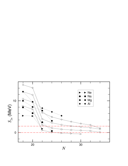
FIG. 19.: The two-neutron separation energies $S_{2n}$ for even-neutron Ne, Na, Mg, and Al nuclei in the drip line region. Open symbols represent the values calculated with the RCHB theory with the NL-SH parameter set, while corresponding solid symbols represent the data available. The horizontal line at 2MeV denotes the upper limit for the possible occurrence of halos.

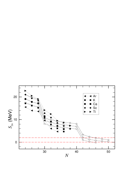
FIG. 20.: Same as Fig.19, but for even Ar, K, Ca, Sc, and Ti nuclei in the drip line region.

Many nuclear physicists are making much effort to search the drip line for heavier elements. A new experiment [32, 33] has been reported that both ³⁷Na and ³⁴Ne are bound, while ³³Ne and ³⁶Na are missed in the experiment. Looking at Fig. 19, the ³⁷Na and ³⁴Ne nuclei lie in the drip line region and approach to the giant halo nuclei. Therefore we suggest that much more experimental effort should be devoted to extend the study in this area and measure the mass to find the possible giant halo nuclei. Similar situation can also be seen in Fig.20 for Ar, K, Ca, Sc and Ti isotopes near the neutron dripline.

V Summary

We have investigated the ground state properties of even-even proton magic O, Ca, Ni, Zr, Sn, and Pb isotopes with the relativistic continuum Hartree-Bogoliubov (RCHB) theory. We have found good agreement with available experimental data for the binding energies and the nuclear radii. We have shown the binding energies, $E_{b}$, two neutron separation energies, $S_{2n}$, and root mean square radii. The predicted neutron drip nuclei are ²⁸O, ⁷²Ca, ⁹⁸Ni, ¹³⁶Zr, ¹⁷⁶Sn, and ²⁶⁶Pb, respectively. Particularly the giant halos in the neutron rich Ca and Zr isotopes close to the neutron drip line are predicted. The giant halo properties in exotic Ca isotopes with $A>60$ is discussed in detail.

Giant neutron halos in exotic Ca isotopes have been studied from the analysis of $S_{2n}$, radii, nucleon density distribution, single particle energy levels, occupation probabilities and the contributions from the continuum. The spin-orbit splitting and the potential diffuseness in Ca isotopes have also been investigated. Summarizing the present investigation, we conclude:

1. Based on the analysis of two-neutron separation energies $S_{2n}$, rms radii, single-particle levels spectra, the orbital occupation, and the contribution of the continuum, giant halo phenomena are suggested to appear in Ca isotopes with A$>$60. Similar phenomena can also be seen for nuclei near the Na or Ar isotopes near the neutron dripline.

2. The neutron drip line nucleus for Ca is ⁷²Ca instead of ⁷⁰Ca, which is caused by the disappearance of the $N=50$ magic number due to the halo effect of the $3s_{1/2}$ orbit.

3. The giant halos developed in these nuclei are due to the pairing correlation and the contribution from the continuum e.g. the $3s_{1/2}$ orbit.

4. The spin-orbit splitting in Ca isotopes decreases monotonically from the proton drip line to the neutron drip line for most cases. This tendency mainly comes from the diffuseness of nuclear potential with the neutron number.

In this paper, the proton magic even-even nuclei from the proton drip line to the neutron drip line are studied in detail in RCHB theory. The important contribution from the continuum due to the pairing correlations has been taken into account. The powerfulness of the RCHB method has been demonstrated for the proton magic nuclei using the assumption of the spherical shape. One of the other important degrees of freedom for the exotic nuclei is the deformation. The theoretical framework for exotic nuclei with the deformation and contribution from continuum are in progress and will be completed soon.

VI Acknowledgements

This work was partly supported by the Major State Basic Research Development Program Under Contract Number G2000077407 and the National Natural Science Foundation of China under Grant No. 10025522, 10047001, and 19935030. J.M. is grateful to RCNP of Osaka University and Physikdepartment, Technische Universität München for their support and warm hospitality, where a part of this work was worked out.

REFERENCES

- [1] I. Tanihata, Prog. Part. Nucl. Phys. 35 (1995)505.
- [2] A.C. Mller, Prog. Part. Nucl. Phys. 46 (2001) 359.
- [3] I. Tanihata et al, Phys. Rev. Lett. 55 (1985) 2676.
- [4] A. Ozawa, T. Kobayashi, T. Suzuki, K. Yoshida, and I. Tanihata, Phys. Rev. Lett. 84 (2000) 5493.
- [5] J.D. Walecka, Ann.Phys. (N.Y.) 83 (1974) 491.
- [6] B.D. Serot and J.D. Walecka, Adv. Nucl. Phys. 16 (1986) 1.
- [7] P. Ring, Prog. Part. Nucl. Phys. 37 (1996) 193.
- [8] H. Kucharek and P. Ring, Z. Phys. A339, 23 (1991).
- [9] J. Meng, and P. Ring, Phys. Rev. Lett. 77 (1996) 3963.
- [10] J. Meng, Nucl. Phys. A635 (1998) 3.
- [11] J. Meng, and P. Ring, Phys. Rev. Lett. 80 (1998) 460.
- [12] J. Meng, H. Toki, and J.Y. Zeng et.al., Phys. Rev. C65(2002)R041302.
- [13] S.A. Fayans, S. V. Tolokonnikov, and D. Zawischa, Phys. Lett. B 491, (2000) 245.
- [14] Soojae Im and J. Meng, Phys. Rev. C 61,(2000) 047302.
- [15] B. Q. Chen et. al., Phys. Lett. B 455, (1999) 13.
- [16] I. Hamamoto, H. Sagawa and X. Z. Zhang, Phys. Rev. C 64, (2001) 024313.
- [17] J. Boguta, A.R. Bodmer, Nucl. Phys. A292 (1977) 413.
- [18] J.F. Berger et al, Nucl. Phys. A428 (1984) 32c.
- [19] M.M. Sharma, M.A. Nagarajan, and P. Ring, Phys. Lett. B312 (1993) 377.
- [20] Y. Sugahara and H. Toki, Nucl. Phys. A579 (1994) 557.
- [21] G. Audi and A. H. Wapstra Nucl. Phys. A 595, (1995) 409.
- [22] M. Fauerbach, D.J. Morriseey, and W. Benenson et.al., Phys. Rev. C 53 (1996) 647.
- [23] D. Guillemaud-Mueller, J. C. Jacmart, and E. Kashy et.al., Phys. Rev. C 41 (1990) 937.
- [24] O. Tarasov, R. Allatt, and J. C. Anegelique et.al., Phys. Lett. B 409 (1997) 64.
- [25] T. Siiskonen, P.O. Lipas, and J. Rikovska, Phys. Rev. C 60 (1999) 034312 and references therein.
- [26] J. Meng and I. Tanihata, Nucl. Phys. A650 (1999) 176.
- [27] J. Dobaczewski, W. Nazarewicz, and T. R. Werner et.al., Phys. Rev. C 53 (1996) 2809.
- [28] S.Q. Zhang, J. Meng, S.-G. Zhou, and J.Y. Zeng, Eur. Phys. J. A 13 (2002) 285.
- [29] M. López-Quelle, N. Van Giai, S. Marcos, and L. N. Savushkin, Phys. Rev. C 61 (2000) 064321.
- [30] G.A. Lalazissis et.al., Phys. Lett. B 418 (1998) 7.
- [31] J. Meng, K.Sugawara-Tanabe, S.Yamaji, P. Ring and A.Arima, Phys. Rev. C58 (1998) R628. J. Meng, K.Sugawara-Tanabe, S.Yamaji, and A.Arima, Phys. Rev. C59 (1998) 154.
- [32] M. Notani et al., Phys. Lett. B 542 (2002) 49.
- [33] S. M. Lukyanov et.al., private communication.