Spherical Relativistic Hartree theory in a Woods-Saxon basis

Abstract

The Woods-Saxon basis has been suggested to replace the widely used harmonic oscillator basis for solving the relativistic mean field (RMF) theory in order to generalize it to study exotic nuclei. As examples, relativistic Hartree theory is solved for spherical nuclei in a Woods-Saxon basis obtained by solving either the Schrödinger equation or the Dirac equation (labelled as SRHSWS and SRHDWS, respectively and SRHWS for both). In SRHDWS, the negative levels in the Dirac Sea must be properly included. The basis in SRHDWS could be smaller than that in SRHSWS which will simplify the deformed problem. The results from SRHWS are compared in detail with those from solving the spherical relativistic Hartree theory in the harmonic oscillator basis (SRHHO) and those in the coordinate space (SRHR). All of these approaches give identical nuclear properties such as total binding energies and root mean square radii for stable nuclei. For exotic nuclei, e.g., ⁷²Ca, SRHWS satisfactorily reproduces the neutron density distribution from SRHR, while SRHHO fails. It is shown that the Woods-Saxon basis can be extended to more complicated situations for exotic nuclei where both deformation and pairing have to be taken into account.

I Introduction

The existence of an average field in atomic nuclei revealed by the exceptional role of the nuclear magic numbers provides the foundation of the nuclear shell model and various mean field approaches Mayer55 ; Bohr69 ; Ring80 . This average field is believed to be approximated most closely by a Woods-Saxon (WS) potential Woods54 either from analyzing the radial dependence of the nuclear force or by deriving it from a microscopic two-body force.

Since the eigenfunctions for the WS potential can not be given analytically, as good approximations for stable nuclei, one often adopts the harmonic oscillator (HO) potential or the square well, in particular the former, in shell model calculations for both spherical Mayer55 and deformed nuclei Nilsson55 . The HO eigenfunctions also often serve as a complete basis in solving equations in both non-relativistic and relativistic mean field approximations, such as the Skyrme Hartree-Fock (SHF), Hartree-Fock-Bogoliubov (HFB), relativistic Hartree (RH) and relativistic Hartree-Bogoliubov (RHB) theories. In these approaches, solution of corresponding equations is transformed to a matrix diagnolization problem which can be easily dealt with.

However, due to the incorrect asymptotic property of the HO wave functions, the expansion in the localized HO basis are not appropriate for the description of drip line nuclei Dobaczewski96 ; Meng96 ; Zhou00 which display many interesting features because of the extremely weakly bound property, e.g., the coupling between bound states and the continuum due to the pairing correlation, large spacial density distributions, possible modifications of shell structure, et al. One must improve the asymptotic behavior of HO wave functions, e.g., by performing a local scaling transformation Stoitsov98 . However, one does not know the scaling parameter beforehand thus the predictive power in this method is lost.

A proper representation to solve the HFB or RHB equations for drip line nuclei is the coordinate space Dobaczewski84 ; Meng96 ; Terasaki96 ; Poeschl97 where wave functions are approximated on a spatial lattice and the continuum is discretized by suitably large box boundary conditions. The HFB method solved in $r$ space can take fully into account all the mean-field effects of the coupling to the continuum Dobaczewski96 ; Meng96 ; Dobaczewski84 ; Belyaev87 . Nevertheless for deformed nuclei, working in $r$ space becomes much more difficult and numerically very sophisticated Zhou00 . Particularly, it become very time consuming when the pairing correlation is included. Therefore much effort is made towards a more efficient solution of HFB or RHB equations, e.g., using natural orbitals Reinhard97 or working on basis-spline Galerkin lattices Oberacker99 , etc..

A reconciler between the HO basis and the $r$ space may be the WS basis because (i) the WS potential represents the nuclear average field more suitably than the HO potential and (ii) in principal there is no localization restrictions in the WS potential. Although analytical wave functions can not be given for the WS potential, one may easily find numerical solutions for a spherical WS potential in the $r$ space by virtue of various effective methods of solving ordinary differential equations NumericalRecipe . One can still use a large box boundary condition to discretize the continuum. These WS wave functions can thus be used as a complete basis for spherical or deformed systems and one finally comes back to the familiar matrix diagnolization problem.

In the present work we restrict the application of this method to nuclei with spherical symmetry which largely facilitates the discussion of basic principles and allows presenting illustrations for the radial dependence of all relevant physical quantities like density distributions. We combine this approach with the relativistic Hartree theory Serot86 which provides a framework for describing the nuclear many body problem as a relativistic system of baryons and mesons and, together with its extensions with deformation and/or pairing included, have been successfully applied in calculations of nuclear matter and properties of finite nuclei throughout the periodic table Reinhard89 ; Ring96 .

The paper is organized as follows. In Sec. II, we give a brief reminder of the formalism of relativistic Hartree theory. The numerical details of solving it in the WS basis are given in Sec. III. In Sec. IV we present our results and compare them with those obtained in the HO basis and in the $r$ space. We also discuss the contribution from negative levels in the Dirac sea in the same section. Finally, the work is summarized in Sec. V.

Throughout the paper, the relativistic Hartree theories solved in the $r$ space, in the HO basis and in the WS basis are abbreviated as “SRHR”, “SRHHO” and “SRHWS” where the first “S” represents “spherical”. We use “SWS” and “DWS” to distinguish the WS basis which is obtained from solving the Schrödinger equation or the Dirac equation with initial WS potentials, respectively. Thus we have “SRHSWS” and “SRHDWS” theories.

II Basic formalism of relativistic Hartree theory

The starting point of the relativistic Hartree theory is a Lagrangian density where nucleons are described as Dirac spinors which interact via the exchange of several mesons ($\sigma$, $\omega$, and $\rho$) and the photon Serot86 ; Reinhard89 ; Ring96 ,

$$\displaystyle{\cal L} = \bar{\psi}_{i}\left(i\hbox to0.0pt{/\hss}\partial-M\right)\psi_{i}+\frac{1}{2}\partial_{\mu}\sigma\partial^{\mu}\sigma-U(\sigma)-g_{\sigma}\bar{\psi}_{i}\sigma\psi_{i}$$ (1)

$$\mbox{}-\frac{1}{4}\Omega_{\mu\nu}\Omega^{\mu\nu}+\frac{1}{2}m_{\omega}^{2}\omega_{\mu}\omega^{\mu}-g_{\omega}\bar{\psi}_{i}\hbox to0.0pt{/\hss}\omega\psi_{i}$$

$$\mbox{}-\frac{1}{4}\vec{R}_{\mu\nu}\vec{R}^{\mu\nu}+\frac{1}{2}m_{\rho}^{2}\vec{\rho}_{\mu}\vec{\rho}^{\mu}-g_{\rho}\bar{\psi}_{i}\hbox to0.0pt{/\hss}\vec{\rho}\vec{\tau}\psi_{i}$$

$$\mbox{}-\frac{1}{4}F_{\mu\nu}F^{\mu\nu}-e\bar{\psi}_{i}\frac{1-\tau_{3}}{2}\hbox to0.0pt{/\hss}A\psi_{i},$$

with the summation convention used and the summation over $i$ runs over all nucleons, $\hbox to0.0pt{/\hss}x\equiv\gamma^{\mu}x_{\mu}=\gamma_{\mu}x^{\mu}$, $M$ the nucleon mass, and $m_{\sigma}$, $g_{\sigma}$, $m_{\omega}$, $g_{\omega}$, $m_{\rho}$, $g_{\rho}$ masses and coupling constants of the respective mesons. The nonlinear self-coupling for the scalar mesons is given by Boguta77

$$U(\sigma)=\dfrac{1}{2}m^{2}_{\sigma}\sigma^{2}+\dfrac{g_{2}}{3}\sigma^{3}+\dfrac{g_{3}}{4}\sigma^{4},$$ (2)

and field tensors for the vector mesons and the photon fields are defined as

$$\left\{\begin{array}[]{rcl}\Omega_{\mu\nu}&=&\partial_{\mu}\omega_{\nu}-\partial_{\nu}\omega_{\mu},\\ \vec{R}_{\mu\nu}&=&\partial_{\mu}\vec{\rho}_{\nu}-\partial_{\nu}\vec{\rho}_{\mu}-g_{\rho}(\vec{\rho}_{\mu}\times\vec{\rho}_{\nu}),\\ F_{\mu\nu}&=&\partial_{\mu}{A}_{\nu}-\partial_{\nu}{A}_{\mu}.\end{array}\right.$$ (6)

The classical variation principle gives the equations of motion for the nucleons, mesons and the photon. As in many applications, we study the ground state properties of nuclei with time reversal symmetry, thus the nucleon spinors are the eigenvectors of the stationary Dirac equation

$$\left[\bm{\alpha}\cdot\bm{p}+V(\bm{r})+\beta(M+S(\bm{r}))\right]\psi_{i}(\bm{r})=\epsilon_{i}\psi_{i}(\bm{r}),$$ (7)

and equations of motion for the mesons and the photon are

$$\left\{\begin{array}[]{rcl}\left(-\Delta+\partial_{\sigma}U(\sigma)\right)\sigma(\bm{r})&=&-g_{\sigma}\rho_{s}(\bm{r}),\\ \left(-\Delta+m_{\omega}^{2}\right)\omega^{0}(\bm{r})&=&g_{\omega}\rho_{v}(\bm{r}),\\ \left(-\Delta+m_{\rho}^{2}\right)\rho^{0}(\bm{r})&=&g_{\rho}\rho_{3}(\bm{r}),\\ -\Delta A^{0}(\bm{r})&=&e\rho_{p}(\bm{r}),\end{array}\right.$$ (12)

where $\omega^{0}$ and $A^{0}$ are time-like components of the vector $\omega$ and the photon fields and $\rho^{0}$ the 3-component of the time-like component of the iso-vector vector $\rho$ meson. Equations (7) and (12) are coupled by the vector and scalar potentials

$$\left\{\begin{array}[]{lll}V(\bm{r})&=&g_{\omega}\omega^{0}(\bm{r})+g_{\rho}\tau_{3}\rho^{0}(\bm{r})+e\dfrac{1-\tau_{3}}{2}A^{0}(\bm{r}),\\ S(\bm{r})&=&g_{\sigma}\sigma(\bm{r}),\\ \end{array}\right.$$ (15)

and various densities

$$\left\{\begin{array}[]{rcl}\rho_{s}(\bm{r})&=&\sum_{i=1}^{A}\bar{\psi}_{i}(\bm{r})\psi_{i}(\bm{r}),\\ \rho_{v}(\bm{r})&=&\sum_{i=1}^{A}\psi_{i}^{\dagger}(\bm{r})\psi_{i}(\bm{r}),\\ \rho_{3}(\bm{r})&=&\sum_{i=1}^{A}\psi_{i}^{\dagger}(\bm{r})\tau_{3}\psi_{i}(\bm{r}),\\ \rho_{c}(\bm{r})&=&\sum_{i=1}^{A}\psi_{i}^{\dagger}(\bm{r})\dfrac{1-\tau_{3}}{2}\psi_{i}(\bm{r}).\end{array}\right.$$ (20)

For spherical nuclei, meson fields and densities depend only on the radial coordinate $r$. The spinor is characterized by the angular momentum quantum numbers ($l$,$j$), $m$, the parity, the isospin $t=\pm 1/2$ (“+” for neutrons and “$-$” for protons), and the radial quantum number $\alpha$. The Dirac spinor has the form

$$\psi_{\alpha\kappa m}(\bm{r},s,t)=\left(\begin{array}[]{c}i\dfrac{G_{\alpha}^{\kappa}(r)}{r}Y^{l}_{jm}(\theta,\phi)\\ -\dfrac{F_{\alpha}^{\kappa}(r)}{r}Y^{\tilde{l}}_{jm}(\theta,\phi)\end{array}\right)\chi_{t_{\alpha}}(t),\ \ j=l\pm\frac{1}{2},$$ (21)

with $G_{\alpha}^{\kappa}(r)/r$ and $F_{\alpha}^{\kappa}(r)/r$ the radial wave functions for the upper and lower components and $Y^{l}_{jm}(\theta,\phi)$ the spin spherical harmonics where $\kappa=(-1)^{j+l+1/2}(j+1/2)$ and $\tilde{l}=l+(-1)^{j+l-1/2}$. The value of $\kappa$ of the upper component is used to label a state both for normal levels in the Fermi sea and for negative ones in the Dirac sea. States with the same $\kappa$ form a “block”. The radial equation of the Dirac spinor, Eq. (7), is reduced as

$$\left\{\begin{array}[]{lll}\epsilon_{\alpha}G_{\alpha}^{\kappa}&=&\left(-\dfrac{\partial}{\partial r}+\dfrac{\kappa}{r}\right)F_{\alpha}^{\kappa}+\left(M+S(r)+V(r)\right)G_{\alpha}^{\kappa},\\ \epsilon_{\alpha}F_{\alpha}^{\kappa}&=&\left(+\dfrac{\partial}{\partial r}+\dfrac{\kappa}{r}\right)G_{\alpha}^{\kappa}-\left(M+S(r)-V(r)\right)F_{\alpha}^{\kappa}.\end{array}\right.$$ (22)

The meson field equations become simply radial Laplace equations of the form

$$\left(-\frac{\partial^{2}}{\partial r^{2}}-\frac{2}{r}\frac{\partial}{\partial r}+m_{\phi}^{2}\right)\phi(r)=s_{\phi}(r).$$ (23)

$m_{\phi}$ are the meson masses for $\phi=\sigma,\omega,\rho$ and zero for the photon. The source terms are

$$s_{\phi}(r)=\left\{\begin{array}[]{ll}-g_{\sigma}\rho_{s}(r)-g_{2}\sigma^{2}(r)-g_{3}\sigma^{3}(r),&\text{for}\ \sigma,\\ g_{\omega}\rho_{v}(r),&\text{for}\ \omega,\\ g_{\rho}\rho_{3}(r),&\text{for}\ \rho,\\ e\rho_{c}(r),&\text{for}\ A,\\ \end{array}\right.$$ (28)

with

$$\left\{\begin{array}[]{lll}4\pi r^{2}\rho_{s}(r)&=&\sum_{i=1}^{A}(|G_{i}(r)|^{2}-|F_{i}(r)|^{2}),\\ 4\pi r^{2}\rho_{v}(r)&=&\sum_{i=1}^{A}(|G_{i}(r)|^{2}+|F_{i}(r)|^{2}),\\ 4\pi r^{2}\rho_{3}(r)&=&\sum_{i=1}^{A}2t_{i}(|G_{i}(r)|^{2}+|F_{i}(r)|^{2}),\\ 4\pi r^{2}\rho_{c}(r)&=&\sum_{i=1}^{A}\left(\frac{1}{2}-t_{i}\right)(|G_{i}(r)|^{2}+|F_{i}(r)|^{2}).\\ \end{array}\right.$$ (33)

Table 1: Dependence of the average single particle energy, root mean square (rms) radius, and $\langle r^{4}\rangle^{1/4}$ on the mesh size $\Delta r$ for the SRHSWS theory. The meson and Coulomb fields are obtained from SRHR calculations with the parameter set NL3, $\Delta r=0.05$ fm, $R_{\text{max}}$ = 30 fm for ¹⁶O and 35 fm for ²⁰⁸Pb. In SRHSWS calculations, the parameter set NL3 is used. For ¹⁶O, $R_{\text{max}}=4r_{0}A^{1/3}=12.8$ fm, $E_{\text{cut}}=300$ MeV. For ²⁰⁸Pb, $R_{\text{max}}=3r_{0}A^{1/3}=22.6$ fm, $E_{\text{cut}}=200$ MeV. The first row gives results from solving the Dirac equation in the coordinate space.

$\Delta r$	$-E_{\text{sp}}/A$	$\langle r^{2}\rangle^{1/2}$	$\langle r^{4}\rangle^{1/4}$	$-E_{\text{sp}}/A$	$\langle r^{2}\rangle^{1/2}$	$\langle r^{4}\rangle^{1/4}$
	16O			208Pb
—	23.0375	2.5945	2.8900	23.3348	5.6315	5.9883
0.05	23.0375	2.5945	2.8900	23.3348	5.6315	5.9883
0.10	23.0376	2.5945	2.8899	23.3348	5.6315	5.9883
0.20	23.0385	2.5941	2.8896	23.3347	5.6315	5.9883
0.30	23.0430	2.5930	2.8889	23.3343	5.6314	5.9883
0.40	23.0420	2.5923	2.8885	23.3334	5.6315	5.9885
0.50	22.9887	2.5949	2.8936	23.3284	5.6319	5.9890

The above coupled equations have been solved in the $r$ space Horowitz81 and in the HO basis Gambhir90 with the no sea and the mean field approximation. Here we depict briefly the procedure of solving these coupled equations. With a set of estimated meson and photon fields, the scalar and vector potentials are calculated and the radial Dirac equation is solved. Thus obtained nucleon wave functions are used to calculate the source term of each radial Laplace equation for mesons and the photon. New meson and photon fields are calculated from solving these Laplace equations. This procedure is iterated until a demanded accuracy is achieved. Laplace equations are usually solved using the Green’s function method Horowitz81 ; Gambhir90 though in Ref. Gambhir90 Laplace equations for mesons are solved in the HO basis. SRHR, SRHHO and SRHWS differ from each other mainly in how to solve the Dirac equation. In the following the numerical solution of the Dirac equation in the WS basis will be presented.

III Solving the Dirac equation in a Woods-Saxon basis and numerical details

III.1 Woods-Saxon basis from solving a Schrödinger equation (the SWS basis)

For the Schrödinger equation with a spherical Woods-Saxon potential

$$V_{\text{WS}}(r)=\left\{\begin{array}[]{ll}\dfrac{V_{0}}{1+e^{(r-R_{0})/a_{0}}},&r<R_{\text{max}},\\ \infty,&r\geq R_{\text{max}},\\ \end{array}\right.$$ (34)

where $R_{\text{max}}$ is introduced for practical reasons to define the box boundary, the eigenfunction can be written as $\phi_{nlm_{l}}(\bm{r})=R_{nl}(r)Y_{lm_{l}}(\theta,\phi)$. Its radial Schrödinger equation is derived as

$$\left[-\dfrac{1}{2M}\left(\dfrac{1}{r^{2}}\dfrac{\partial}{\partial r}r^{2}\dfrac{\partial}{\partial r}-\dfrac{l(l+1)}{r^{2}}\right)+V_{\text{WS}}(r)\right]R_{nl}(r)$$

$$=\ E_{nl}R_{nl}(r).$$ (35)

Table 2: Dependence of the average single particle energy, rms radius, and $\langle r^{4}\rangle^{1/4}$ on the difference $\Delta n=\tilde{n}_{\text{max}}-n_{\text{max}}$ for the SRHSWS theory. The meson and Coulomb fields are obtained from SRHR calculations with the parameter set NL3, $\Delta r=0.05$ fm, $R_{\text{max}}$ = 30 fm for ¹⁶O and 35 fm for ²⁰⁸Pb. In SRHSWS calculations, the parameter set NL3 is used. For ¹⁶O, $R_{\text{max}}=4r_{0}A^{1/3}=12.8$ fm. For ²⁰⁸Pb, $R_{\text{max}}=3r_{0}A^{1/3}=22.6$ fm.

$\Delta n$	$-E_{\text{sp}}/A$	$\langle r^{2}\rangle^{1/2}$	$\langle r^{4}\rangle^{1/4}$	$-E_{\text{sp}}/A$	$\langle r^{2}\rangle^{1/2}$	$\langle r^{4}\rangle^{1/4}$
	16O: $E_{\text{cut}}=100$ MeV			208Pb: $E_{\text{cut}}=100$ MeV
1	23.0382	2.5947	2.8920	23.3344	5.6315	5.9884
3	23.0326	2.5949	2.8913	23.3341	5.6315	5.9884
5	23.0298	2.5952	2.8915	23.3340	5.6315	5.9884
7	23.0290	2.5953	2.8915	23.3340	5.6315	5.9884
9	23.0289	2.5953	2.8915	23.3340	5.6315	5.9884
	16O: $E_{\text{cut}}=300$ MeV			208Pb: $E_{\text{cut}}=200$ MeV
1	23.0375	2.5945	2.8999	23.3348	5.6315	5.9883
3	23.0375	2.5945	2.8999	23.3348	5.6315	5.9883
5	23.0375	2.5945	2.8999	23.3347	5.6315	5.9883
7	23.0375	2.5945	2.8999	23.3347	5.6315	5.9883
9	23.0375	2.5945	2.8999	23.3347	5.6315	5.9883

Equation (35) is solved on a discretized radial mesh with a mesh size $\Delta r$. $R_{\text{max}}$ ($\Delta r$) should be chosen larger (smaller) enough to make sure that the final results do not depend on it. The radial wave functions thus obtained form a complete basis,

$$\left\{R_{nl}(r);n=0,1,\cdots;l=0,1,\cdots,n\right\},$$ (36)

in terms of which the radial part of the upper and the lower components of the Dirac spinor in Eq. (22) are expanded respectively as

$$\left\{\begin{array}[]{l}\displaystyle G_{\alpha}^{\kappa}(r)=-i\sum_{n=0}^{n_{\text{max}}}g_{\alpha n}rR_{nl}(r),\\ \displaystyle F_{\alpha}^{\kappa}(r)=-i\sum_{\tilde{n}=0}^{\tilde{n}_{\text{max}}}f_{\alpha\tilde{n}}rR_{\tilde{n}\tilde{l}}(r).\\ \end{array}\right.$$ (37)

The radial Dirac equation, Eq. (22), is transformed into the WS basis as

$$\left(\begin{array}[]{cc}{\cal A}_{mn}&{\cal B}_{m\tilde{n}}\\ {\cal C}_{\tilde{m}n}&{\cal D}_{\tilde{m}\tilde{n}}\\ \end{array}\right)\left(\begin{array}[]{c}g_{\alpha n}\\ f_{\alpha\tilde{n}}\\ \end{array}\right)=\epsilon_{\alpha}\left(\begin{array}[]{c}g_{\alpha n}\\ f_{\alpha\tilde{n}}\\ \end{array}\right),$$ (38)

where the matrix elements are calculated as follows

$$\left\{\begin{array}[]{l}\displaystyle{\cal A}_{mn}=\int_{0}^{R_{\text{max}}}r^{2}drR_{ml}(r)\left(V(r)+S(r)+M\right)R_{nl}(r),\\ \displaystyle{\cal B}_{m\tilde{n}}=\int_{0}^{R_{\text{max}}}r^{2}drR_{ml}(r)\left(+\frac{\partial}{\partial r}-\frac{\kappa_{\alpha}-1}{r}\right)R_{\tilde{n}\tilde{l}}(r),\\ \displaystyle{\cal C}_{\tilde{m}n}=\int_{0}^{R_{\text{max}}}r^{2}drR_{\tilde{m}\tilde{l}}(r)\left(-\frac{\partial}{\partial r}-\frac{\kappa_{\alpha}+1}{r}\right)R_{nl}(r),\\ \displaystyle{\cal D}_{\tilde{m}\tilde{n}}=\int_{0}^{R_{\text{max}}}r^{2}drR_{\tilde{m}\tilde{l}}(r)\left(V(r)-S(r)-M\right)R_{\tilde{n}\tilde{l}}(r).\\ \end{array}\right.$$ (39)

In practical calculations, an energy cutoff $E_{\text{cut}}$ (relative to the nucleon mass $M$) is used to determine the cutoff of the radial quantum number $n_{\text{max}}$ for each block. In the expansion of the corresponding lower component, we take $\tilde{n}_{\text{max}}=n_{\text{max}}+\Delta n$ with $\Delta n\geq 1$ in order to avoid spurious states Gambhir90 .

Figure 1: Deviations of the average single particle energy $E^{\text{sp}}/A$ (the upper panel), rms radius $\langle r\rangle^{1/2}$ (the middle panel), and $\langle r^{4}\rangle^{1/4}$ (the lower panel) of ¹⁶O from the standard results versus the cutoff energy $E_{\text{cut}}$ with different box size $R_{\text{max}}$ for the SRHSWS theory. The meson and Coulomb fields are obtained from SRHR calculations with the parameter set NL3, $\Delta r=0.05$ fm, $R_{\text{max}}$ = 30 fm. In SRHSWS calculations, the parameter set NL3 is used. For $E_{\text{cut}}$ = 100, 200, 300, 400 MeV, the approximate maximum principal quantum number in each basis, $N_{\text{max}}=2n_{\text{max}}+l$, is given on the top of the plot.

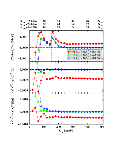
Figure 2: Deviations of the average single particle energy $E^{\text{sp}}/A$ (the upper panel), rms radius $\langle r\rangle^{1/2}$ (the middle panel), and $\langle r^{4}\rangle^{1/4}$ (the lower panel) of ²⁰⁸Pb from the standard results versus the cutoff energy $E_{\text{cut}}$ with different box size $R_{\text{max}}$ for the SRHSWS theory. The meson and Coulomb fields are obtained from SRHR calculations with the parameter set NL3, $\Delta r=0.05$ fm, $R_{\text{max}}$ = 35 fm. In SRHSWS calculations, the parameter set NL3 is used. For $E_{\text{cut}}$ = 100, 200, 300, 400 MeV, the approximate maximum principal quantum number in each basis, $N_{\text{max}}=2n_{\text{max}}+l$, is given on the top of the plot.

The following Woods-Saxon parameters have been used according to Ref. Heyde99

$$\left\{\begin{array}[]{l}V_{0}=(-51\pm 33(N-Z)/A)\text{ MeV},\\ R_{0}=1.27A^{1/3}\text{ fm},\ a_{0}=0.67\text{ fm},\\ \end{array}\right.$$ (40)

where ‘+’ is for the neutron and ‘$-$’ for the proton. As expected, the dependence of final results on the initial WS potential is almost negligible. For example, a variation of $V_{0}$ by 50% gives differences in total binding energies by less than 0.1% and charge radii by less than 0.5% for ¹⁶O, ⁴⁸Ca and ²⁰⁸Pb. Such situation is also checked to be true for the other two parameters in the WS potential, $R_{0}$ and $a_{0}$.

III.2 Woods-Saxon basis from solving a Dirac equation (the DWS basis)

The radial Dirac equation, Eq. (22), may be solved in the $r$ space Horowitz81 with Woods-Saxon-like potentials for $V_{0}(r)\pm S_{0}(r)$ Koepf91 within a spherical box of the size $R_{\text{max}}$, together with the spherical spinor which gives a complete WS basis

$$\left\{\left[\epsilon_{n\kappa m}^{0},\psi_{n\kappa m}^{0}(\bm{r},s,t)\right];\epsilon_{n\kappa m}^{0}\gtrless 0\right\},$$ (41)

with $n=0,1,\cdots$, $\kappa=\pm 1,\pm 2,\cdots$, and $m=-j_{\kappa},\cdots,j_{\kappa}$. $\psi_{n\kappa m}^{0}(\bm{r},s,t)$ takes the form of Eq. (21). We note that states both in the Fermi sea and in the Dirac sea should be included in the basis for the completeness. The nucleon wave function, Eq. (21), can be expanded in terms of this set of basis as

$$\psi_{\alpha\kappa m}(\bm{r},s,t)=\sum_{n=0}^{n_{\text{max}}}c_{\alpha n}\psi_{n\kappa m}^{0}(\bm{r},s,t),$$ (42)

where $n_{\text{max}}=n_{\text{max}}^{+}+n_{\text{max}}^{-}+1$ and the summation is over normal levels in the Fermi sea for $0\leq n\leq n_{\text{max}}^{+}$ and over negative levels in the Dirac sea for $n_{\text{max}}^{+}+1\leq n\leq n_{\text{max}}$. The negative states is obtained with the same method as the positive ones Horowitz81 . In this WS basis, the Dirac equation, Eq. (7), turns out to be

$$c_{\alpha m}\epsilon_{m}^{0}+\sum_{n=0}^{n_{\text{max}}}c_{\alpha n}H^{\prime}_{mn}=\epsilon_{\alpha}c_{\alpha m},\ m=1,\cdots,n_{\text{max}},$$ (43)

with

$$H^{\prime}_{mn} = \left\langle\psi_{m}^{0}(\bm{r})\right|\left[\Delta V(\bm{r})+\beta\Delta S(\bm{r})\right]\left|\psi_{n}^{0}(\bm{r})\right\rangle$$ (44)

$$= \int_{0}^{R_{\text{max}}}drG_{m}^{0}(r)\left[\Delta V(r)+\Delta S(r)\right]G_{n}^{0}(r)$$

$$+ \int_{0}^{R_{\text{max}}}drF_{m}^{0}(r)\left[\Delta V(r)-\Delta S(r)\right]F_{n}^{0}(r),$$

where $\Delta V(\bm{r})=V(\bm{r})-V_{0}(\bm{r})$ and $\Delta S(\bm{r})=S(\bm{r})-S_{0}(\bm{r})$. The angular, spin, and isospin quantum numbers are omitted for brevity.

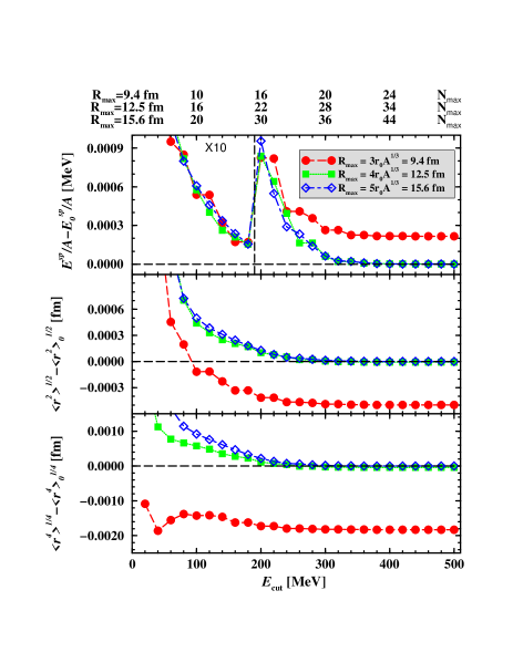
Figure 3: Deviations of the average single particle energy $E^{\text{sp}}/A$ (the upper panel), rms radius $\langle r\rangle^{1/2}$ (the middle panel), and $\langle r^{4}\rangle^{1/4}$ (the lower panel) of ¹⁶O from the standard results versus the cutoff energy $E_{\text{cut}}$ with different box size $R_{\text{max}}$ for the SRHDWS theory. The meson and Coulomb fields are obtained from SRHR calculations with the parameter set NL3, $\Delta r=0.05$ fm, $R_{\text{max}}$ = 30 fm. In SRHDWS calculations, the parameter set NL3 is used. For $E_{\text{cut}}$ = 100, 200, 300, 400 MeV, the approximate maximum principal quantum number in each basis, $N_{\text{max}}=2n_{\text{max}}+l$, is given on the top of the plot.

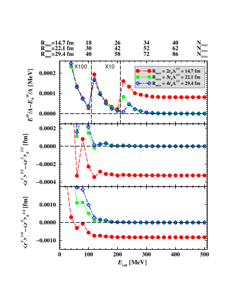
Figure 4: Deviations of the average single particle energy $E^{\text{sp}}/A$ (the upper panel), rms radius $\langle r\rangle^{1/2}$ (the middle panel), and $\langle r^{4}\rangle^{1/4}$ (the lower panel) of ²⁰⁸Pb from the standard results versus the cutoff energy $E_{\text{cut}}$ with different box size $R_{\text{max}}$ for the SRHDWS theory. The meson and Coulomb fields are obtained from SRHR calculations with the parameter set NL3, $\Delta r=0.05$ fm, $R_{\text{max}}$ = 35 fm. In SRHDWS calculations, the parameter set NL3 is used. For $E_{\text{cut}}$ = 100, 200, 300, 400 MeV, the approximate maximum principal quantum number in each basis, $N_{\text{max}}=2n_{\text{max}}+l$, is given on the top of the plot.

It should be mentioned that Eq. (22) can be solved directly in the $r$ space with the same method of generating the DWS basis. It is our aim to test the validity of an efficient solution not only for the spherical RH model but also for its extension to include the deformation and/or the pairing correlation. In fact, if only the SRH theory is concerned, this procedure is just a replacement of the direct solution in the $r$ space by a diagnolization of a matrix with some complication introduced by the fact that contributions from states in the Dirac sea must be included.

An energy cutoff $E_{\text{cut}}$ (relative to the nucleon mass $M$) and the cutoff of radial quantum numbers $n_{\text{max}}^{+}$ are applied to normal levels alternatively according to practical convenience. For the initial Woods-Saxon potentials $V_{0}(r)\pm S_{0}(r)$, we follow Ref. Koepf91 .

III.3 Comparison with the $r$-space method

In order to check the validity of solving the Dirac equation in the WS basis and to provide numerical experiences for future applications, we compare results of ¹⁶O and ²⁰⁸Pb from solving the Dirac equation in the WS basis and those from solving the same equation in the coordinate space. The latter is the most accurate method of solving the Dirac equation for realistic nuclei up to now thus is used as a standard here. The scalar and vector potentials in the Dirac equation are provided by very accurate SRHR calculations with the parameter set NL3 for the Lagrangian, the mesh size $\Delta r$ = 0.05 fm, the box size $R_{\text{max}}$ = 30 fm for ¹⁶O and $R_{\text{max}}$ = 35 fm for ²⁰⁸Pb. Then with thus obtained $S(r)$ and $V(r)$, the Dirac equation is solved in the coordinate space and in the WS basis with also the parameter set NL3.

To compare results only from solving the Dirac equation avoids errors from other numerical procedures, e.g., the error from the iteration and that from solving the Laplace equations. For the same reason, what we compare between these two methods is not the binding energy which contains the contribution from mesons but the average single particle energy $E^{\text{sp}}/A$. $E^{\text{sp}}=\sum_{i}\epsilon_{i}$ where $\epsilon_{i}$ is the single particle energy and the summation over all occupied states for both neutrons and protons. We also compare the rms radius $\langle r^{2}\rangle^{1/2}$ and $\langle r^{4}\rangle^{1/4}$. The radius $\langle r^{4}\rangle^{1/4}$ reflects the nucleon densities in the tail more than the rms radius.

Table 1 presents the dependence of results of the Dirac equation in the SWS basis on the mesh size $\Delta r$. With $\Delta r$ decreasing, results in the SWS basis approach the standard results, i.e., those in the $r$ space. $\Delta r$ = 0.1 fm gives results accurate enough. The dependence on the box size $R_{\text{max}}$ and on the basis size determined by $E_{\text{cut}}$ are investigated and shown in Figs. 1 and 2 where the deviations of the average single particle energy $E^{\text{sp}}/A$, the rms radius $\langle r^{2}\rangle^{1/2}$ and $\langle r^{4}\rangle^{1/4}$ from the standards are plotted versus $E_{\text{cut}}$ for different $R_{\text{max}}$. If $R_{\text{max}}$ is not large enough, it is difficult to approach the standard results. For example, when $R_{\text{max}}=3r_{0}A^{1/3}=9.4$ fm and $E_{\text{cut}}$ = 300 MeV for ¹⁶O (correspondingly, $N_{\text{max}}\sim 20$), the results seem converge, but the discrepancy of the average single particle energy from the standard one remains 0.1 keV. So one must use a large enough box with the size $R_{\text{max}}$ around $4r_{0}A^{1/3}$ for light nuclei and $3r_{0}A^{1/3}$ for heavy ones. It is interesting that the convergence of the results does not depend on $N_{\text{max}}$ but only on $E_{\text{cut}}$. For ¹⁶O (²⁰⁸Pb), the results converge to the standard ones at $\sim$ 300 (400) MeV. From Figs. 1 and 2, we find the radius $\langle r^{4}\rangle^{1/4}$ also converges very well which implies that nucleon densities could be calculated accurately even for large $r$.

We have made similar investigations for results in the DWS basis and similar conclusions are made. For instances, the deviations of the average single particle energy $E^{\text{sp}}/A$, the rms radius $\langle r^{2}\rangle^{1/2}$ and $\langle r^{4}\rangle^{1/4}$ from the standards are plotted versus $E_{\text{cut}}$ for different $R_{\text{max}}$ in Figs. 3 and 4.

Table 3: Dependence of the single particle energy, rms radius, and $\langle r^{4}\rangle^{1/4}$ on the maximum principal quantum number, $N_{\text{max}}^{-}=2n_{\text{max}}^{-}+l$, for the SRHDWS theory. The meson and Coulomb fields are obtained from SRHR calculations with the parameter set NL3, $\Delta r=0.05$ fm, $R_{\text{max}}$ = 30 fm for ¹⁶O and 35 fm for ²⁰⁸Pb. In SRHDWS calculations, the parameter set NL3 is used. For ¹⁶O, $R_{\text{max}}=4r_{0}A^{1/3}=12.5$ fm, $E_{\text{cut}}=300$ MeV for positive states. For ²⁰⁸Pb, $R_{\text{max}}=3r_{0}A^{1/3}=22.1$ fm, $E_{\text{cut}}=200$ MeV for positive states.

$\tilde{N}_{\text{max}}$	$-E_{\text{sp}}/A$	$\langle r^{2}\rangle^{1/2}$	$\langle r^{4}\rangle^{1/4}$	$-E_{\text{sp}}/A$	$\langle r^{2}\rangle^{1/2}$	$\langle r^{4}\rangle^{1/4}$
	16O			208Pb
no	23.1129	2.5912	2.8859	23.3331	5.6314	5.9889
0	23.1077	2.5916	2.8861	23.3329	5.6314	5.9889
2	23.0762	2.5939	2.8889	23.3316	5.6315	5.9890
4	23.0617	2.5942	2.8893	23.3304	5.6317	5.9892
6	23.0439	2.5946	2.8898	23.3299	5.6318	5.9893
8	23.0385	2.5946	2.8899	23.3294	5.6319	5.9893
10	23.0376	2.5946	2.8899	23.3292	5.6319	5.9894
12	23.0375	2.5946	2.8899	23.3291	5.6319	5.9899
14	23.0375	2.5946	2.8899	23.3290	5.6319	5.9894
16	23.0375	2.5946	2.8899	23.3290	5.6319	5.9894
18	23.0375	2.5946	2.8899	23.3289	5.6319	5.9893
20	23.0375	2.5946	2.8899	23.3288	5.6319	5.9893
22	23.0375	2.5946	2.8899	23.3287	5.6319	5.9893
30	23.0375	2.5946	2.8899	23.3287	5.6319	5.9893

In the expansion of the nucleon wave function, Eq. (42), one has to take into account not only the levels in the Fermi sea but also those in the Dirac sea because they form a complete basis together. Now the question arises how many levels in the Dirac sea one has to take into account. In the calculations in Figs. 3 and 4, we have used $n_{\text{max}}^{-}=n_{\text{max}}^{+}$ with $n_{\text{max}}^{+}$ determined by $E_{\text{cut}}$. In Table 3, the dependence of the average single particle energy, the rms radius $\langle r^{2}\rangle^{1/2}$ and $\langle r^{4}\rangle^{1/4}$ on $N_{\text{max}}^{-}=2n_{\text{max}}^{-}+l$ — a cutoff on the principal quantum number of levels in the Dirac sea — are given for ¹⁶O and ²⁰⁸Pb. From Table 3, we find a merit of solving the Dirac equation in the DWS basis: the number of negative states included in the basis could be much smaller that that of the positive states. Let take ¹⁶O as an example, $R_{\text{max}}=4r_{0}A^{1/3}$ and $E_{\text{cut}}$ = 300 MeV for positive states correspond to $N_{\text{max}}^{+}\sim$ 28. But for negative states, $N_{\text{max}}^{-}$ = 10 gives very accurate results, e.g., the discrepancy of $E^{\text{sp}}/A$ from the standard is smaller than 0.1 keV. This will significantly simplify the deformed problem by decreasing the matrix dimension compared to solve the Dirac equation in the SWS basis.

The above investigations are somehow academic. In practical applications, it is not necessary to go to the accuracy around keV in the single particle energy or 10^-4 fm in the radius. So in the following calculations, we will use $R_{\text{max}}$ = 20 fm, $\Delta r$ = 0.1 fm and $E_{\text{cut}}$ = 60$\sim$80 MeV for heavy and light nuclei which give reasonable accuracies both for the binding energy and the radius. This set of cutoff’s corresponds approximately $N_{\text{max}}=2n_{\text{max}}+l\sim 25$ where $l$ is the orbital angular momentum of relevant state.

IV Results and discussions

In this section we present results of SRHWS. Since our main aim is to show the virtues of SRHWS compared to SRHHO and SRHR, we do not include pairing correlations and restrict our study to doubly magic or magic nuclei only. If not specified, the parameter set NLSH is used for the Lagrangian, $R_{\text{max}}$ = 20 fm and $\Delta r$ = 0.1 fm throughout this section. Other parameter sets for the Lagrangian do not change the conclusion here. In SRHDWS, the number of normal levels in the Fermi sea and that of negative ones in the Dirac sea are the same for convenience, i.e., $n_{\text{max}}^{+}=n_{\text{max}}^{-}$. For SRHHO, $\hbar\omega_{0}=41A^{-1/3}$ has been used and cutoff’s of the expansion for fermions and bosons are the same, i.e., $N_{\text{F}}=N_{\text{B}}\equiv N_{\text{max}}$.

IV.1 Bulk properties of stable nuclei from different SRH theories

In Table 4, the binding energy per nucleon ($E/A$) and neutron, proton and charge radii ($r_{\text{n}}$, $r_{\text{p}}$ and $r_{\text{c}}$) of some typical spherical nuclei are presented which are calculated from the present available codes, including SRHR, SRHSWS, SRHDWS, SRHHO. Available data Audi95 ; DeVries87 are also included for comparison. We use approximately the same $N_{\text{max}}$ in the SRHHO as that in the SRHWS which is determined by $E_{\text{cut}}$.

Generally speaking, for each studied nucleus, the four approaches give almost the same results with an accuracy within 0.1% with few exceptions where the differences are still less than 0.3%. They are in excellent agreement with available data.

Table 4: The binding energy per nucleon and neutron, proton and charge radii of some typical spherical nuclei. The parameter set NLSH is used for the Lagrangian. $R_{\text{max}}$ = 20 fm and $\Delta r$ = 0.1 fm for SRHR and SRHWS. $\hbar\omega_{0}=41A^{-1/3}$ for SRHHO. Numbers in brackets in the second column give $E_{\text{cut}}$ for SRHWS and $N_{\text{max}}$ for SRHHO. Data for $E/A$ and $r_{\text{c}}$ are taken from Ref. Audi95 and Ref. DeVries87 , respectively. Energy is in MeV and radius in fm.

Nucleus		$E/A$	$r_{\text{n}}$	$r_{\text{p}}$	$r_{\text{c}}$
16O	SRHR	$-8.022$	2.551	2.578	2.699
	SRHSWS (80)	$-8.022$	2.554	2.581	2.702
	SRHDWS (80)	$-8.014$	2.553	2.580	2.701
	SRHHO (25)	$-8.034$	2.551	2.577	2.699
	Experiment	$-7.976$			2.693
40Ca	SRHR	$-8.500$	3.311	3.359	3.452
	SRHSWS (80)	$-8.499$	3.310	3.358	3.452
	SRHDWS (80)	$-8.497$	3.312	3.359	3.453
	SRHHO (25)	$-8.514$	3.310	3.358	3.452
	Experiment	$-8.551$			3.478
48Ca	SRHR	$-8.644$	3.586	3.369	3.463
	SRHSWS (80)	$-8.646$	3.583	3.368	3.461
	SRHDWS (80)	$-8.639$	3.586	3.371	3.464
	SRHHO (25)	$-8.659$	3.584	3.368	3.462
	Experiment	$-8.666$			3.479
56Ni	SRHR	$-8.634$	3.582	3.630	3.717
	SRHSWS (80)	$-8.640$	3.580	3.628	3.715
	SRHDWS (80)	$-8.625$	3.585	2.633	3.720
	SRHHO (25)	$-8.650$	3.581	3.629	3.716
	Experiment	$-8.345$
90Zr	SRHR	$-8.677$	4.294	4.186	4.262
	SRHSWS (75)	$-8.677$	4.295	4.187	4.263
	SRHDWS (75)	$-8.672$	4.295	4.187	4.262
	SRHHO (25)	$-8.693$	4.293	4.185	4.261
	Experiment	$-8.710$			4.270
118Sn	SRHR	$-8.466$	4.743	4.553	4.623
	SRHSWS (70)	$-8.466$	4.743	4.554	4.624
	SRHDWS (70)	$-8.460$	4.743	4.554	4.624
	SRHHO (25)	$-8.482$	4.741	4.552	4.622
	Experiment	$-8.517$			4.641
132Sn	SRHR	$-8.377$	4.964	4.636	4.704
	SRHSWS (70)	$-8.377$	4.964	4.637	4.704
	SRHDWS (70)	$-8.370$	4.964	4.637	4.706
	SRHHO (25)	$-8.393$	4.963	4.635	4.703
	Experiment	$-8.355$
208Pb	SRHR	$-7.885$	5.713	5.447	5.505
	SRHSWS (60)	$-7.886$	5.712	5.447	5.505
	SRHDWS (60)	$-7.874$	5.712	5.448	5.506
	SRHHO (25)	$-7.900$	5.711	5.445	5.504
	Experiment	$-7.868$			5.504

With the same parameters of spatial lattice $R_{\text{max}}$ and $\Delta r$, SRHWS should reproduce results of SRHR when $E_{\text{cut}}$ (or $N_{\text{max}}$) is large enough. This is justified in Table 4. One find exactly coincident results between SRHSWS and SRHR for most of the studied nuclei. The remaining differences and those between SRHDWS and SRHR could be diminished by increasing $E_{\text{cut}}$.

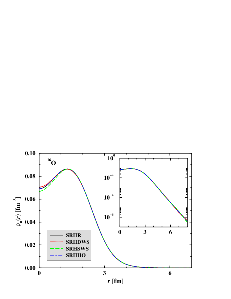
Figure 5: Neutron density distributions for ¹⁶O from different SRH approaches. The parameter set NLSH is used for the Lagrangian. $R_{\text{max}}$ = 20 fm and $\Delta r$ = 0.1 fm for SRHR and SRHWS. $E_{\text{cut}}=80$ MeV for SRHWS. Correspondingly, $N_{\text{max}}$ = 25 for SRHHO. In SRHDWS, the number of levels in the Dirac sea included in each block is the same as that of normal levels which is determined by $E_{\text{cut}}$. The inset presents logarithmic densities.

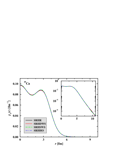
Figure 6: Neutron density distributions for ⁴⁸Ca from different SRH approaches. The parameter set NLSH is used for the Lagrangian. $R_{\text{max}}$ = 20 fm and $\Delta r$ = 0.1 fm for SRHR and SRHWS. $E_{\text{cut}}=80$ MeV for SRHWS. Correspondingly, $N_{\text{max}}$ = 25 for SRHHO. In SRHDWS, the number of levels in the Dirac sea included in each block is the same as that of normal levels which is determined by $E_{\text{cut}}$. The inset presents logarithmic densities.

Figure 7: Neutron density distributions for ²⁰⁸Pb from different SRH approaches. The parameter set NLSH is used for the Lagrangian. $R_{\text{max}}$ = 20 fm and $\Delta r$ = 0.1 fm for SRHR and SRHWS. $E_{\text{cut}}=60$ MeV for SRHWS. Correspondingly, $N_{\text{max}}$ = 25 for SRHHO. In SRHDWS, the number of levels in the Dirac sea included in each block is the same as that of normal levels which is determined by $E_{\text{cut}}$. The inset presents logarithmic densities.

In Figures 5, 6 and 7, the neutron density distributions are compared between SRHR, SRHSWS, SRHDWS, and SRHHO, in which ¹⁶O, ⁴⁸Ca and ²⁰⁸Pb are chosen as examples. The calculation details are the same as Table 4. For these stable nuclei, all these SRH methods are valid and all calculations are in excellent agreement with each other from the central to outer region of each nucleus. Tiny differences in the central region do not affect the physical observables like the binding energy or nuclear radius as is seen in Table 4. Furthermore, these differences could also be decreased by increasing $E_{\text{cut}}$ or $N_{\text{max}}$.

From the above discussions, it is clear that SRHWS is equivalent to SRHR and SRHHO for stable nuclei. Thus we conclude that Woods-Saxon basis provide another possibility to solve (non-)relativistic mean field theory.

IV.2 Neutron density distributions for ⁷²Ca in different SRH theories

As we already discussed in the introduction, one of the merits of SRHR against SRHHO is its proper description of exotic nuclei. In this subsection, we will demonstrate the equivalence between SRHWS and SRHR when reasonably large $E_{\text{cut}}$ is applied in SRHWS.

In order to see the results for the unstable nuclei near the neutron drip line, the neutron density distribution for ⁷²Ca is studied here. The nucleus ⁷²Ca is predicted to be the last bound calcium isotope Im00 ; Hamamoto01 ; Zhang02 ; Meng02 . Since it is not a doubly magic nucleus, there might be some uncertainty in present results due to the lack of inclusion of pairing correlations. However, as we stressed in the beginning of this section, the main aim here is to show the virtue of SRHWS compared to SRHHO, it is very unlikely that the pairing would change our conclusion qualitatively.

Table 5: Convergence study for ⁷²Ca. The parameter set NLSH is used for the Lagrangian. $\Delta r$ = 0.1 fm for SRHR and SRHWS. $E_{\text{cut}}=75$ MeV for SRHWS. Energy is in MeV and radius in fm.

	$E/A$	$r_{\text{n}}$	$r_{\text{p}}$	$\lambda_{\text{n}}$
$R_{\text{max}}$	SRHR
20	6.482	4.656	3.639	$-$0.191
25	6.483	4.723	3.639	$-$0.221
30	6.484	4.773	3.639	$-$0.228
35	6.484	4.807	3.639	$-$0.229
$R_{\text{max}}$	SRHSWS
20	6.481	4.663	3.639	$-$0.206
25	6.482	4.726	3.639	$-$0.231
30	6.483	4.774	3.639	$-$0.237
35	6.483	4.803	3.639	$-$0.238
$R_{\text{max}}$	SRHDWS
20	6.474	4.662	3.641	$-$0.163
25	6.475	4.733	3.641	$-$0.197
30	6.475	4.789	3.640	$-$0.205
35	6.475	4.828	3.640	$-$0.206
$N_{\text{max}}$	SRHHO
25	6.489	4.577	3.639	$-$0.054
31	6.492	4.605	3.639	$-$0.128
37	6.494	4.628	3.639	$-$0.166
43	6.494	4.649	3.639	$-$0.189

For stable nuclei, it has been shown that $R_{\text{max}}\sim$ 20 fm is large enough. For drip line nuclei, the dependence of the results on $R_{\text{max}}$ for ⁷²Ca is presented in Table 5. For both SRHR and SRHWS, $\Delta r$ = 0.1 fm and $R_{\text{max}}$ = 20, 25, 30 and 35 fm have been adopted respectively. The energy cutoff $E_{\text{cut}}$ = 75 MeV is used to SRHWS. In SRHR and SRHWS calculations, the neutron rms radius $r_{\text{n}}$ and Fermi energy $\lambda_{\text{n}}$ of ⁷²Ca converge around $R_{\text{max}}$ = 35 fm while a independence of the binding energy per nucleon $E/A$ and proton rms radius $r_{\text{p}}$ on the box size can be seen. These sets of parameters in SRHWS, $E_{\text{cut}}$ = 75 MeV and $R_{\text{max}}$ = 20, 25, 30 and 35 fm, correspond to cutoff’s on principal quantum number $N_{\text{max}}$ = 25, 31, 37 and 43 which are used in SRHHO calculations in order to make fair comparisons between SRHWS and SRHHO. Similar as those from SRHR and SRHWS, $E/A$ and $r_{\text{p}}$ depend little on $N_{\text{max}}$ in SRHHO. However, the neutron rms radius $r_{\text{n}}$ increases with $N_{\text{max}}$ steadily, which shows a much slower convergence. As it is based on a complete basis, SRHHO can reach convergence of $r_{\text{n}}$ if $N_{\text{max}}$ is large enough. From Table 5, one finds that for the same $N_{\text{max}}$ (or equivalent $R_{\text{max}}$), a difference of $\Delta r_{\text{n}}\approx$ 0.2 fm between SRHHO and SRHWS (SRHR) can be seen. From the slow convergence of $r_{\text{n}}$ with $N_{\text{max}}$ in SRHHO ($\Delta N_{\text{max}}$ = 6 gives $\Delta r_{\text{n}}\approx$ 0.02 fm), we can estimate the lower limit of the $N_{\text{max}}$ as $N_{\text{max}}\approx$ 90 in order to give $r_{\text{n}}$ = 4.8 fm in SRHR or SRHWS.

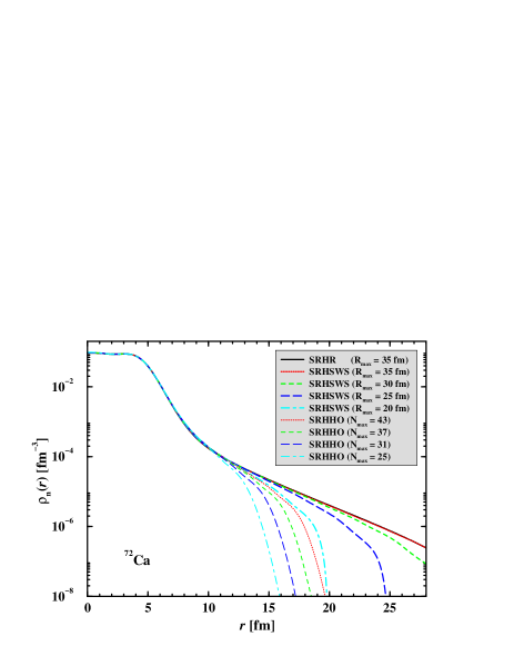
Figure 8: Comparison of density distributions for ⁷²Ca from SRHR, SRHSWS and SRHHO. The parameter set NLSH is used for the Lagrangian. $\Delta r$ = 0.1 fm for SRHR and SRHSWS. $E_{\text{cut}}$ = 75 MeV and $R_{\text{max}}$ = 20 (thick dot-dashed curve), 25 (thick long-dashed curve), 30 (thick dashed curve) and 35 fm (thick dotted curve) for SRHSWS. These sets of cutoff’s correspond to cutoff’s in principal quantum number $N_{\text{max}}$ = 25 (thin dot-dashed curve), 31 (thin long-dashed curve), 37 (thin dashed curve) and 43 (thin dotted curve) which are used in SRHHO calculations. The density distribution from SRHR are almost identical with that from SRHSWS with the same box size. For brevity, only $\rho_{n}(r)$ from SRHR with $R_{\text{max}}$ = 35 fm (thick solid line) is displayed here which covers the curve corresponding to $\rho_{n}(r)$ from SRHSWS with $R_{\text{max}}$ = 35 fm (thick dotted curve).

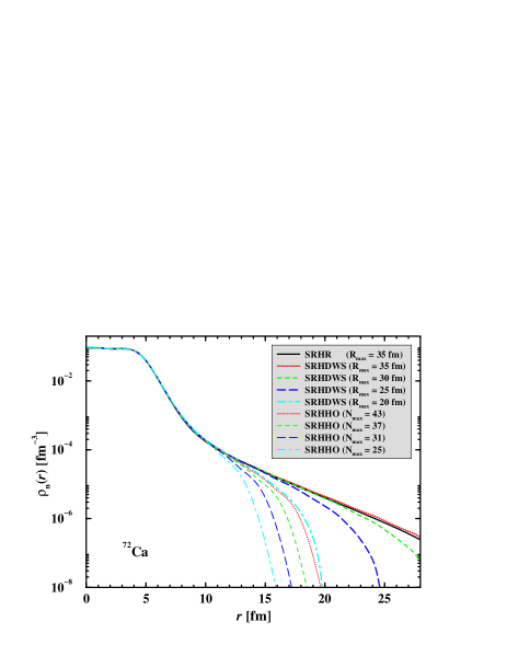
Figure 9: Comparison of density distributions for ⁷²Ca from SRHR, SRHDWS and SRHHO. The parameter set NLSH is used for the Lagrangian. $\Delta r$ = 0.1 fm for SRHR and SRHDWS. $E_{\text{cut}}$ = 75 MeV and $R_{\text{max}}$ = 20 (thick dot-dashed curve), 25 (thick long-dashed curve), 30 (thick dashed curve) and 35 fm (thick dotted curve) for SRHDWS. In SRHHO calculations, $N_{\text{max}}$ = 25 (thin dot-dashed curve), 31 (thin long-dashed curve), 37 (thin dashed curve) and 43 (thin dotted curve) are used. The density distribution from SRHR are very close to that from SRHSWS with the same box size. For brevity, only $\rho_{n}(r)$ from SRHR with $R_{\text{max}}$ = 35 fm (thick solid line) is displayed here.

We compare the neutron density distribution of ⁷²Ca from different SRH approaches in Figs. 8 and 9. With the same box size, the density distribution from SRHR are almost identical with those from SRHWS, which indicates the equivalence between SRHWS and SRHR. For brevity, only $\rho_{\text{n}}(r)$ from SRHR with $R_{\text{max}}$ = 35 fm is displayed in Figs. 8 or 9 which covers the curve corresponding to $\rho_{n}(r)$ from SRHSWS with $R_{\text{max}}$ = 35 fm in Fig. 8. On the other hand, $\rho_{\text{n}}(r)$ from SRHHO even with $N_{\text{max}}$ = 43 fails to reproduce the result of SRHR due to the localization property of HO potential. In addition, with the same $N_{\text{max}}$, the spatial extension of $\rho_{\text{n}}(r)$ from SRHWS are always larger than that from SRHHO. The variational tendency of the curve $\rho_{\text{n}}(r)\sim r$ also explains different convergence behaviors of $r_{\text{n}}$ in SRHWS and SRHHO as given in Table 5. With increasing $R_{\text{max}}$, the $\rho_{\text{n}}(r)$ in SRHWS has the correct asymptotic behavior while that in SRHHO decay too quickly.

This result is very encouraging and tell us that even the long tail (or halo) behavior in neutron density distribution for nuclei near the drip line can be described by SRHSWS as well as SRHR, if pairing correlations is incorporated properly.

IV.3 Contribution from negative levels in the SRHDWS theory

In the expansion of the nucleon wave function, Eq. (42), one has to take into account not only the levels in the Fermi sea but also those in the Dirac sea because they form a complete basis together. We study the effects of negative levels and give results of an example, ¹⁶O, in Table 6. Firstly, without negative levels included, the nucleus is over bound and the nuclear size is smaller as seen from Table 6. Secondly, in contrary to the case with negative levels included, the calculated nuclear properties depend on the initial potentials very much if no negative levels included.

It should be noted that the contribution from negative levels depends on the initial Woods-Saxon potentials for generating the DWS basis. So do the cutoff $N_{\text{max}}$ or $E_{\text{cut}}$ for convergence. If the initial Woods-Saxon potential is exactly identical to the converged potentials, the matrix in Eq. (43) is diagonal, negative states do not contribute because of the no sea approximation. Positive states can also be chosen as less as possible, e.g., $1s_{1/2}$, $1p_{3/2}$ and $1p_{1/2}$ are enough for ¹⁶O. From the third column corresponding to $V_{0}$ = 72 MeV in Table 6, one finds that the initial nuclear potential for the Dirac equation proposed in Ref. Koepf91 is a good choice for SRHDWS as the negative states only contribute $\sim$ 1.25 % to both $E/A$ and $r_{\text{rms}}$. If we change the initial potentials, e.g., by changing $V_{0}$ by 25%, much larger contributions from negative states are found in Table 6.

Table 6: Effects of negative levels on bulk properties in SRHDWS for ¹⁶O. The parameter set for the Lagrangian is NLSH, $R_{\text{max}}=20$ fm, $\Delta r=0.1$ fm, and $N^{+}_{\text{max}}=25$. For the initial Woods-Saxon like potentials, parameters in Ref. Koepf91 are used except for $V_{0}$ which is specified in the table. The left value in each entry gives the result without negative levels included and the right one that with $N^{-}_{\text{max}}$ = 25. Energy is in MeV and radius in fm.

	$V_{0}=54$ MeV	$V_{0}=72$ MeV	$V_{0}=90$ MeV
$E/A$	8.547 $|$ 8.013	8.117 $|$ 8.015	8.427 $|$ 8.012
$r_{\text{rms}}$	2.385 $|$ 2.568	2.531 $|$ 2.567	2.610 $|$ 2.567

Table 7: Contribution of negative levels in the Dirac sea to the single nucleon wave functions of ¹⁶O in SRHDWS. For each single particle levels, $\sum|c^{-}_{n}|^{2}$ in the expansion Eq. (42) is presented. The parameter set for the Lagrangian is NLSH, $R_{\text{max}}=20$ fm and $\Delta r=0.1$ fm and $N^{+}_{\text{max}}=N^{-}_{\text{max}}=25$. For the initial Woods-Saxon like potentials, the parameters in Ref. Koepf91 are used except for $V_{0}$ which is specified in the table. The binding energy per nucleon and nuclear radius for each calculation is presented in Table 6.

Level	$V_{0}=54$ MeV	$V_{0}=72$ MeV	$V_{0}=90$ MeV
N$1s_{1/2}$	9.15$\times 10^{-5}$	3.48$\times 10^{-5}$	3.44$\times 10^{-4}$
N$1p_{3/2}$	5.32$\times 10^{-5}$	6.05$\times 10^{-5}$	3.69$\times 10^{-4}$
N$1p_{1/2}$	4.01$\times 10^{-4}$	1.06$\times 10^{-5}$	8.80$\times 10^{-4}$
P$1s_{1/2}$	1.92$\times 10^{-4}$	4.92$\times 10^{-5}$	4.89$\times 10^{-5}$
P$1p_{3/2}$	1.17$\times 10^{-4}$	3.27$\times 10^{-5}$	8.07$\times 10^{-5}$
P$1p_{1/2}$	8.09$\times 10^{-4}$	2.08$\times 10^{-4}$	2.38$\times 10^{-5}$

In order to know the contribution of negative levels in the Dirac sea to the wave function, the value of $\sum_{n}|c_{n}^{-}|^{2}$ in the expansion, Eq. (42) has been given in Table 7 for occupied states of ¹⁶O. We note that the nucleon wave function is normalized to one. It can be seen that a small component from negative states in the wave functions, about $10^{-4\sim-5}$, contributes to the physical observables such as $E/A$ and $r_{\text{rms}}$ by the magnitude of 1%$\sim$10% as seen from Table 6. Again we notice that the initial Woods-Saxon potentials differ more from the converged ones, the larger is the contribution from negative levels.

V Summary

We have solved the spherical relativistic Hartree theory in the Woods-Saxon basis (SRHWS). The Woods-Saxon basis is obtained by solving either the Schrödinger equation (SRHSWS) or the Dirac equation (SRHDWS). Formalism and numerical details for both cases are presented. The WS basis in the SRHDWS theory could be very smaller than that in the SRHSWS theory. This will largely facilitate solving the deformed problem.

The results from SRHWS are compared with those from solving the spherical relativistic Hartree theory in the harmonic oscillator basis, SRHHO, and those in the coordinate space, SRHR. For stable nuclei, all approaches give identical results for properties such as total binding energies and the neutron, proton and charge rms radii as well as neutron density distributions.

For neutron drip line nuclei, e.g. ⁷²Ca, which has a very small neutron Fermi energy $\lambda_{\text{n}}\sim 0.2$ MeV, both SRHR and SRHWS easily approach convergence by increasing box size while SRHHO does not. Furthermore, SRHWS can satisfactorily reproduce the neutron density distribution from SRHR, but SRHHO fails with similar cutoff’s.

In SRHDWS calculations, the negative levels in the Dirac Sea must be included in the basis in terms of which nucleon wave functions are expanded. We studied in detail the effects and contributions of negative states. Without negative levels included, the calculated nuclear properties depend on the initial potentials very much. A small component from negative states in the wave functions, about $10^{-4\sim-5}$, contributes to the physical observables such as $E/A$ and $r_{\text{rms}}$ by the magnitude of 1%$\sim$10%. When the initial potentials differ more from the converged ones, the contribution from negative levels becomes more important.

We conclude that the Woods-Saxon basis provides a reconciler between the harmonic oscillator basis and the coordinate space which may be used to describe exotic nuclei both properly and efficiently.

The extension of spherical relativistic Hartree theory in the Woods-Saxon basis to deformed cases with pairing included is in progress.

- (1) M. G. Mayer and J. H. D. Jensen, Elementary Theory of Nuclear Shell Struture (Wiley, New York, 1955).
- (2) A. Bohr and B. R. Mottelson, Nuclear Structure, Vol. I (Benjamin, New York, 1969).
- (3) P. Ring and P. Schuck, The Nuclear Many-Body Problem (Springer Verlag, Berlin, 1980).
- (4) R. D. Woods and D. S. Saxon, Phys. Rev. 95, 577 (1954).
- (5) S. G. Nilsson, Mat. Fys. Medd. Dan. Vid. Selsk. 29, No.16 (1955).
- (6) J. Dobaczewski, W. Nazarewicz, T. R. Werner, J.-F. Berger, C. R. Chinn, and J. Dechargé, Phys. Rev. C 53, 2809 (1996).
- (7) J. Meng and P. Ring, Phys. Rev. Lett. 77, 3963 (1996); J. Meng, Nucl. Phys. A635, 3 (1998); J. Meng and P. Ring, Phys. Rev. Lett. 80, 460 (1998).
- (8) S.-G. Zhou, J. Meng, S. Yamaji and S. C. Yang, Chin. Phys. Lett. 17, 717 (2000).
- (9) M. V. Stoitsov, P. Ring, D. Vretenar, and G. A. Lalazissis, Phys. Rev. C 58, 2086 (1998); M. V. Stoitsov, W. Nazarewicz, and S. Pittel, Phys. Rev. C 58, 2092 (1998).
- (10) J. Dobaczewski, H. Flocard, and J. Treiner, Nucl. Phys. A422, 103 (1984).
- (11) J. Terasaki, P.-H. Heenen, H. Flocard, and P. Bonche, Nucl. Phys. A600, 371 (1996); J. Terasaki, H. Flocard, P.-H. Heenen, and P. Bonche, ibid, A621, 706 (1997).
- (12) W. Pöschl, D. Vretenar, G. A. Lalazissis, and P. Ring, Phys. Rev. Lett. 79, 3841 (1997).
- (13) S. T. Belyaev, A. V. Smirnov, S. V. Tolokonnikov, and S. A. Fayans, Yad. Fiz. 45, 1263 (1987) [Sov. J. Nucl. Phys. 45, 783 (1987)].
- (14) P.-G. Reinhard, M. Bender, K. Rutz, and J. A. Maruhn, Z. Phys. A 358, 277 (1997).
- (15) V. E. Oberacker and A. S. Umar, Proceedings of the International Symposium on Perspectives in Nuclear Physics (World Scientific, Singapore, 1999).
- (16) W. H. Press, S. A. Teukolsky, W. T. Vetterling, and B. P. Flannery, Numerical Recipes in Fortran 77 (2nd Ed.) (Cambridge University Press, 1992).
- (17) B. D. Serot and J. D. Walecka, Adv. Nucl. Phys. 16, 1 (1986).
- (18) P.-G. Reinhard, Rep. Prog. Phys. 52, 439 (1989).
- (19) P. Ring, Prog. Part. Nucl. Phys. 37 (1996) 193; ibid, 46, 165 (2001).
- (20) J. Boguta and A. R. Bodmer, Nucl. Phys. A 292, 413 (1977).
- (21) C. J. Horowitz and B. D. Serot, Nucl. Phys. A368, 503 (1981).
- (22) Y. K. Gambhir, P. Ring and A. Thimet, Ann. Phys. (NY) 198, 132 (1990).
- (23) W. Koepf and P. Ring, Z. Phys. A 339, 81 (1991).
- (24) K. Heyde, Basis ideas and concepts in nuclear physics, 2nd Ed. (IoP Publishing, Bristol and Philadelphia, 1999).
- (25) G. Audi and A. H. Wapstra, Nucl. Phys. A595, 409(1995).
- (26) H. De Vries, C. W. De Jager and C. De Vries, At. Data Nucl. Data Tables 36, 495 (1987).
- (27) S. Im and J. Meng, Phys. Rev. C 61, 047302 (2000).
- (28) I. Hamamoto, H. Sagawa and X. Z. Zhang, Phys. Rev. C 63, 024313 (2001).
- (29) S.-Q. Zhang, J. Meng, S.-G. Zhou and J.-Y. Zeng, Chin. Phys. Lett. 19, 312 (2002).
- (30) J. Meng, H. Toki, J. Y. Zeng, S. Q. Zhang and S.-G. Zhou, Phys. Rev. C 65, 041302(R) (2002).