Real stabilization method for nuclear single particle resonances

Abstract

We develop the real stabilization method within the framework of the relativistic mean field (RMF) model. With the self-consistent nuclear potentials from the RMF model, the real stabilization method is used to study single-particle resonant states in spherical nuclei. As examples, the energies, widths and wave functions of low-lying neutron resonant states in ¹²⁰Sn are obtained. These results are compared with those from the scattering phase shift method and the analytic continuation in the coupling constant approach and satisfactory agreements are found.

I Introduction

The investigation of continuum and resonant states is an important subject in quantum physics. In recent years, there has been an increasing interest in the exploration of nuclear single particle states in the continuum. The construction of the radioactive ion beam facilities makes it possible to study exotic nuclei with unusual N/Z ratios. In these nuclei, the Fermi surface is usually close to the particle continuum, thus the contribution of the continuum and/or resonances being essential for exotic nuclear phenomena Bulgac80 ; Dobaczewski84 ; Dobaczewski96 ; Meng96 ; Poeschl97 ; Meng98 . It has been also revealed that the contribution of the continuum to the giant resonances mainly comes from single-particle resonant states Curutchet89 ; Cao02 .

For the theoretical determination of resonant parameters (the energy and the width), several bound-state-like methods have been developed. The complex scaling method (CSM) describes the discrete bound and resonant states on the same footing Kato06 . In this method, a complex coordinate scaling is introduced to rotate the continuum into the complex energy plane and the wave functions of resonant states, but not scattering states, are transformed into square-integrable functions Kruppa88 . Although it involves the solution of a complex eigenvalue problem which causes some difficulties in practice, the CSM has been widely and successfully used to study resonances in atomic and molecular systems Reinhardt82 ; Ho83 ; Moiseyev98 and atomic nuclei Gyarmati86 ; Kruppa88 ; Kruppa97 ; Arai06 ; Kato06 . The analytical continuation in the coupling constant (ACCC) approach is based on an intuitive idea that a resonant state can be lowered to be bound when the potential becomes more attractive or equivalently the coupling constant stronger, thus a resonant state being related to a series of bound states via an analytical continuation in the coupling constant Kukulin77 ; Kukulin79 ; Kukulin89 . Combined with the cluster model, the ACCC approach has been used to calculate the resonant energies and widths in some light nuclei Tanaka97 ; Tanaka99 . An attempt to explore the unbound states by the ACCC approach within relativistic mean field (RMF) model was first made in Ref. Yang01 where resonant parameters of some low lying resonant states in ¹⁶O and ⁴⁸Ca obtained from the ACCC calculations are comparable with available data. The wave functions of nuclear resonant states were also determined by the ACCC method where the bound states are obtained by solving either the Schrödinger equation with a Woods-Saxon potential Cattapan00 or the Dirac equation with self-consistent RMF potentials Zhang04 .

The real stabilization method (RSM) is another bound-state-like method Hazi70 . The equation of motion of the system in question is solved in a basis Hazi70 or a box Maier80 of finite sizes, thus a bound state problem being always imposed. The RSM uses the fact that the energy of a “resonant” state is stable against changes of the sizes of the basis or the box. It has been used to calculate the resonance parameters in elastic and inelastic scattering processes Fels71 ; Fels72 . Some efforts have also been made in order to calculate more efficiently resonance parameters with the RSM Taylor76 ; Mandelshtam93 ; Mandelshtam94 ; Kruppa99 . In this work, we investigate single particle resonances in atomic nuclei by combining the RSM and the relativistic mean field (RMF) model.

The paper is organized as follows. In Sec. II we give briefly the formalism for the RSM and the RMF model. The numerical details, the results for ¹²⁰Sn and discussions are given in Sec. III. Finally we give a brief summary.

II Formalism of the RMF model and the RSM

II.1 The relativistic mean field model

The basic ansatz of the relativistic mean field (RMF) model is a Lagrangian density where nucleons are described as Dirac spinors which interact via the exchange of several mesons ($\sigma$, $\omega$, and $\rho$) and the photon Serot86 ; Reinhard89 ; Ring96 ; Vretenar05 ; Meng06 ,

$$\displaystyle{\cal L} = \bar{\psi}_{i}\left(i\hbox to0.0pt{/\hss}\partial-M\right)\psi_{i}+\frac{1}{2}\partial_{\mu}\sigma\partial^{\mu}\sigma-U(\sigma)-g_{\sigma}\bar{\psi}_{i}\sigma\psi_{i}$$ (1)

$$\mbox{}-\frac{1}{4}\Omega_{\mu\nu}\Omega^{\mu\nu}+\frac{1}{2}m_{\omega}^{2}\omega_{\mu}\omega^{\mu}-g_{\omega}\bar{\psi}_{i}\hbox to0.0pt{/\hss}{\mbox{\boldmath$\omega$}}\psi_{i}$$

$$\mbox{}-\frac{1}{4}\vec{R}_{\mu\nu}\vec{R}^{\mu\nu}+\frac{1}{2}m_{\rho}^{2}\vec{\rho}_{\mu}\vec{\rho}^{\mu}-g_{\rho}\bar{\psi}_{i}\hbox to0.0pt{/\hss}\vec{{\mbox{\boldmath$\rho$}}}\vec{\tau}\psi_{i}$$

$$\mbox{}-\frac{1}{4}F_{\mu\nu}F^{\mu\nu}-e\bar{\psi}_{i}\frac{1-\tau_{3}}{2}\hbox to0.0pt{/\hss}{\bf A}\psi_{i},$$

where the summation convention is used and the summation over $i$ runs over all nucleons, $\hbox to0.0pt{/\hss}x\equiv\gamma^{\mu}x_{\mu}=\gamma_{\mu}x^{\mu}$, $M$ the nucleon mass, and $m_{\sigma}$, $g_{\sigma}$, $m_{\omega}$, $g_{\omega}$, $m_{\rho}$, $g_{\rho}$ masses and coupling constants of the respective mesons. The nonlinear self-coupling for the scalar mesons is given by Boguta77

$$U(\sigma)=\dfrac{1}{2}m^{2}_{\sigma}\sigma^{2}+\dfrac{g_{2}}{3}\sigma^{3}+\dfrac{g_{3}}{4}\sigma^{4},$$ (2)

and field tensors for the vector mesons and the photon fields are defined as

$$\left\{\begin{array}[]{rcl}\Omega_{\mu\nu}&=&\partial_{\mu}\omega_{\nu}-\partial_{\nu}\omega_{\mu},\\ \vec{R}_{\mu\nu}&=&\partial_{\mu}\vec{\rho}_{\nu}-\partial_{\nu}\vec{\rho}_{\mu}-g_{\rho}(\vec{\rho}_{\mu}\times\vec{\rho}_{\nu}),\\ F_{\mu\nu}&=&\partial_{\mu}{A}_{\nu}-\partial_{\nu}{A}_{\mu}.\end{array}\right.$$ (6)

The classical variation principle gives equations of motion for the nucleon, mesons and the photon. As in many applications, we study the ground state properties of nuclei with time reversal symmetry, thus the nucleon spinors are the eigenvectors of the stationary Dirac equation

$$\left[\bm{\alpha}\cdot\bm{p}+V(\bm{r})+\beta(M+S(\bm{r}))\right]\psi_{i}(\bm{r})=\epsilon_{i}\psi_{i}(\bm{r}),$$ (7)

and equations of motion for mesons and the photon are

$$\left\{\begin{array}[]{rcl}\left(-\Delta+\partial_{\sigma}U(\sigma)\right)\sigma(\bm{r})&=&-g_{\sigma}\rho_{s}(\bm{r}),\\ \left(-\Delta+m_{\omega}^{2}\right)\omega^{0}(\bm{r})&=&g_{\omega}\rho_{v}(\bm{r}),\\ \left(-\Delta+m_{\rho}^{2}\right)\rho^{0}(\bm{r})&=&g_{\rho}\rho_{3}(\bm{r}),\\ -\Delta A^{0}(\bm{r})&=&e\rho_{p}(\bm{r}),\end{array}\right.$$ (12)

where $\omega^{0}$ and $A^{0}$ are time-like components of the vector $\omega$ and the photon fields and $\rho^{0}$ the 3-component of the time-like component of the iso-vector vector $\rho$ meson. Equations (7) and (12) are coupled to each other by the vector and scalar potentials

$$\left\{\begin{array}[]{lll}V(\bm{r})&=&g_{\omega}\omega^{0}(\bm{r})+g_{\rho}\tau_{3}\rho^{0}(\bm{r})+e\dfrac{1-\tau_{3}}{2}A^{0}(\bm{r}),\\ S(\bm{r})&=&g_{\sigma}\sigma(\bm{r}),\\ \end{array}\right.$$ (15)

and various densities

$$\left\{\begin{array}[]{rcl}\rho_{s}(\bm{r})&=&\sum_{i=1}^{A}\bar{\psi}_{i}(\bm{r})\psi_{i}(\bm{r}),\\ \rho_{v}(\bm{r})&=&\sum_{i=1}^{A}\psi_{i}^{\dagger}(\bm{r})\psi_{i}(\bm{r}),\\ \rho_{3}(\bm{r})&=&\sum_{i=1}^{A}\psi_{i}^{\dagger}(\bm{r})\tau_{3}\psi_{i}(\bm{r}),\\ \rho_{c}(\bm{r})&=&\sum_{i=1}^{A}\psi_{i}^{\dagger}(\bm{r})\dfrac{1-\tau_{3}}{2}\psi_{i}(\bm{r}).\end{array}\right.$$ (20)

For spherical nuclei, meson fields and densities depend only on the radial coordinate $r$, the Dirac spinor reads

$$\psi_{\alpha\kappa m}(\bm{r},s,t)=\left(\begin{array}[]{c}i\dfrac{G_{\alpha}^{\kappa}(r)}{r}Y^{l}_{jm}(\theta,\phi,s)\\ -\dfrac{F_{\alpha}^{\kappa}(r)}{r}Y^{\tilde{l}}_{jm}(\theta,\phi,s)\end{array}\right)\chi_{t_{\alpha}}(t),\ \ j=l\pm\frac{1}{2},$$ (21)

with $Y^{l}_{jm}(\theta,\phi)$ the spin spherical harmonics. The radial equation of the Dirac spinor, Eq. (7), is reduced as

$$\left\{\begin{array}[]{lll}\epsilon_{\alpha}G_{\alpha}^{\kappa}&=&\left(-\dfrac{\partial}{\partial r}+\dfrac{\kappa}{r}\right)F_{\alpha}^{\kappa}+\left(M+S(r)+V(r)\right)G_{\alpha}^{\kappa},\\ \epsilon_{\alpha}F_{\alpha}^{\kappa}&=&\left(+\dfrac{\partial}{\partial r}+\dfrac{\kappa}{r}\right)G_{\alpha}^{\kappa}-\left(M+S(r)-V(r)\right)F_{\alpha}^{\kappa}.\end{array}\right.$$ (22)

The meson field equations become simply radial Laplace equations of the form

$$\left(-\frac{\partial^{2}}{\partial r^{2}}-\frac{2}{r}\frac{\partial}{\partial r}+m_{\phi}^{2}\right)\phi(r)=s_{\phi}(r).$$ (23)

$m_{\phi}$ are the meson masses for $\phi=\sigma,\omega,\rho$ and zero for the photon. The source terms are

$$s_{\phi}(r)=\left\{\begin{array}[]{ll}-g_{\sigma}\rho_{s}(r)-g_{2}\sigma^{2}(r)-g_{3}\sigma^{3}(r),&\text{for}\ \sigma,\\ g_{\omega}\rho_{v}(r),&\text{for}\ \omega,\\ g_{\rho}\rho_{3}(r),&\text{for}\ \rho,\\ e\rho_{c}(r),&\text{for}\ A,\\ \end{array}\right.$$ (28)

with

$$\left\{\begin{array}[]{lll}4\pi r^{2}\rho_{s}(r)&=&\sum_{i=1}^{A}(|G_{i}(r)|^{2}-|F_{i}(r)|^{2}),\\ 4\pi r^{2}\rho_{v}(r)&=&\sum_{i=1}^{A}(|G_{i}(r)|^{2}+|F_{i}(r)|^{2}),\\ 4\pi r^{2}\rho_{3}(r)&=&\sum_{i=1}^{A}2t_{i}(|G_{i}(r)|^{2}+|F_{i}(r)|^{2}),\\ 4\pi r^{2}\rho_{c}(r)&=&\sum_{i=1}^{A}\left(\frac{1}{2}-t_{i}\right)(|G_{i}(r)|^{2}+|F_{i}(r)|^{2}).\\ \end{array}\right.$$ (33)

The above coupled equations can be solved iteratively in $r$ space Horowitz81 or in the harmonic oscillator basis Gambhir90 using the no sea and the mean field approximations.

II.2 The real stabilization method in coordinate space

With the self consistent vector and scalar potentials $V(r)$ and $S(r)$, the Dirac equation (22) is solved in a spherical box of the size $R_{\mathrm{max}}$ under the box boundary condition, and thus the continuum is discretized. When $R_{\mathrm{max}}$ is large enough, the energy of a bound state does not change with $R_{\mathrm{max}}$. In the continuum region, there are some states stable against the size of the box, i.e., the energy of each of such states is almost constant with changing $R_{\mathrm{max}}$; such stable states correspond to resonances.

The resonant parameters, $E_{\gamma}$ and $\Gamma$, may be obtained by fitting the energy $E$ and the phase shift $\eta(E)$ in an energy range around a resonance to the following formula Hazi70 ,

$$\eta_{l}(E)=\eta_{l,\mathrm{pot}}(E)+\tan^{-1}\left(\frac{\Gamma/2}{E-E_{\gamma}}\right).$$ (34)

The phase shift $\eta_{l}(E)$ can be calculated as Zhang07

$$\tan\left(\eta_{l}-\frac{l\pi}{2}\right)=-\frac{\int^{R_{\mathrm{max}}}_{0}\chi_{l}(r)\left[E-H(r)\right]f(r)\sin krdr}{\int^{R_{\mathrm{max}}}_{0}\chi_{l}(r)\left[E-H(r)\right]f(r)\cos krdr},$$ (35)

with $f(r)$ satisfying $f(r)\rightarrow 1$ when $r\rightarrow\infty$ and $f(0)=f^{\prime}(0)=0$. However, Eq. (35) converges very slowly with the box size due to the influence of the non zero centrifugal potential at large ${R_{\mathrm{max}}}$ Zhang07 .

In the present work, we use a simpler method proposed by Maier et al. Maier80 in which it’s not necessary to calculate the phase shift. The resonance energy is determined by the condition $\partial^{2}E/\partial R^{2}_{\mathrm{max}}$ = 0 and the corresponding box size is labeled as $\bar{R}_{\mathrm{max}}$, i.e., $E_{\gamma}=E(\bar{R}_{\mathrm{max}})$. The width is evaluated from the stability behavior of the positive energy state against the box size around $\bar{R}_{\mathrm{max}}$.

When $r$ is large enough, the nuclear potentials $S(r)$ and $V(r)$ vanish, $G(r)/r$ satisfy

$$\frac{d^{2}G}{dr^{2}}+\left(\alpha^{2}-\frac{\kappa(\kappa+1)}{r^{2}}\right)G=0,$$ (36)

with $\alpha^{2}=E^{2}-M^{2}$. The general solution reads

$$G(r)\propto\alpha r\left[\cos\eta_{l}\ j_{l}(\alpha r)-\sin\eta_{l}\ n_{l}(\alpha r)\right],$$ (37)

When $r\rightarrow\infty$, $G(r)\propto\sin(\alpha r-\frac{l\pi}{2}+\eta_{l})$. Therefore when $R_{\mathrm{max}}$ is large enough,

$$\alpha R_{\mathrm{max}}-\frac{l\pi}{2}+\eta_{l}=n\pi.$$ (38)

Under the assumption that the phase shift from the potential scattering $\eta_{l,\mathrm{pot}}(E)$ varies slowly with respect to the box size, i.e, $\partial\eta_{l,\mathrm{pot}}/\partial R_{\mathrm{max}}\sim 0$, one derives from Eqs. (34) and (38) the formula,

$$\Gamma=\frac{2\sqrt{E_{\gamma}^{2}+2E_{\gamma}M}}{-(E_{\gamma}+M)\bar{R}_{\mathrm{max}}-(E_{\gamma}^{2}+2E_{\gamma}M)\left[\partial E/\partial R_{\mathrm{max}}|_{\bar{R}_{\mathrm{max}}}\right]^{-1}}.$$ (39)

In the non-relativistic limit, $E_{\gamma}\ll M$, Eq. (39) is reduced to

$$\Gamma=\frac{2\sqrt{2E_{\gamma}/M}}{-\bar{R}_{\mathrm{max}}-2E_{\gamma}\left[dE/dR_{\mathrm{max}}|_{\bar{R}_{\mathrm{max}}}\right]^{-1}},$$ (40)

which is essentially the same as Eq. (8) in Ref. Maier80 except for that here natural units with $\hbar=c=1$ is used.

III Results and Disscusion

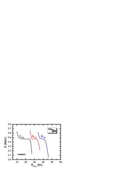
Figure 1: Positive energy $\nu$i_13/2 states in ¹²⁰Sn under different box boundary conditions.

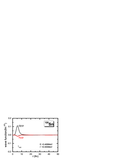
Figure 2: The radial wave function for the neutron $\nu$i_13/2 resonant state in ¹²⁰Sn.

In this section we present the results of the RSM in the framework of the RMF model. In our calculation, we use for the Lagrangian density the effective interactions PK1 Long04 and NL3 Lalazissis97 . We change the size of the box in a large range (7 fm $<R_{\mathrm{max}}<$ 60 fm if not specified) in order to find not only narrow resonances but also wide ones. We take ¹²⁰Sn as an example and compare the results for neutron resonances from the RSM with those from the ACCC approach Zhang04 and the scattering phase shift method Sandulescu03 .

By examining the stability of low lying positive energy states against the size of the box $R_{\mathrm{max}}$, we find that except for s state, there are neutron resonances in ¹²⁰Sn with the orbital angular momentum $l$ up to 6.

The narrowest resonance is an i_13/2 state which lies at about 3.45 MeV above the threshold. The positive energy $\nu$i_13/2 states in a box of different sizes are shown in Fig. 1. With the box size $R_{\mathrm{max}}$ increasing, the lowest $\nu$i_13/2 state first falls down quickly then its energy becomes constant in a large region of $R_{\mathrm{max}}$. After it crosses with the second lowest $\nu$i_13/2 state at around $R_{\mathrm{max}}=25$ fm, the lowest one falls down again. Similar level-crossings occur regularly at larger $R_{\mathrm{max}}$. This stability behavior implies that there is a narrow $\nu$i_13/2 resonant state with approximate energy 3.45 MeV. The resonant energy 3.469 MeV and $\bar{R}_{\mathrm{max}}=20.1$ fm are obtained under the condition $\partial^{2}E/\partial R^{2}_{\mathrm{max}}$ = 0 from the first $E\sim R_{\mathrm{max}}$ curve (labeled as “1i_13/2”) in Fig. 1. The width 0.003 MeV are obtained from Eq. (39). One of the approximations made in deriving Eq. (39) is $R_{\mathrm{max}}$ should be large. We next examine the dependence of the resonant parameters on the box size by calculating $E_{\gamma}$ and $\Gamma$ from other $E\sim R_{\mathrm{max}}$ curves with larger $R_{\mathrm{max}}$. For this purpose the calculations with $R_{\mathrm{max}}$ up to 65 fm are carried out. The results are given in Table 1. The energy is almost a constant with increasing $\bar{R}_{\mathrm{max}}$. The variation between the widths obtained from adjacent $E\sim R_{\mathrm{max}}$ curves decreases with $\bar{R}_{\mathrm{max}}$ and is about 1% at $\bar{R}_{\mathrm{max}}\sim 63$ fm. For other resonant states presented in this work, we also make similar investigations. Once it converges to within 1%, the value of the width is assigned to a resonant state. The wave function of the resonant state $\nu$i_13/2 is given in Fig. 2. From this figure one can find that this state is almost localized inside the nucleus which is consistent with the small width $\Gamma$.

Table 1: Energies and widths of the single neutron resonant state i_13/2 in ¹²⁰Sn from different $E\sim R_{\mathrm{max}}$ curves (cf. Fig. 1). $\bar{R}_{\mathrm{max}}$ is in fm and $E_{\gamma}$ and $\Gamma$ are in MeV.

$\bar{R}_{\mathrm{max}}$	$E_{\gamma}$	100$\times\Gamma$	$\bar{R}_{\mathrm{max}}$	$E_{\gamma}$	100$\times\Gamma$
20.1	3.4688	0.327	47.2	3.4686	0.470
30.3	3.4686	0.426	55.3	3.4685	0.478
38.9	3.4686	0.456	63.2	3.4686	0.483

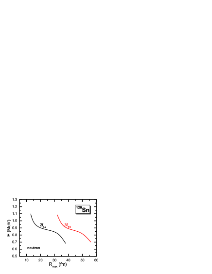
Figure 3: Positive energy $\nu$f_5/2 states in ¹²⁰Sn under different box boundary conditions.

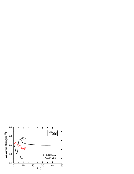
Figure 4: The radial wave function for the neutron $\nu$f_5/2 resonant state in ¹²⁰Sn.

Although it lies below the state $\nu$i_13/2, the resonant state $\nu$f_5/2 is about an order of magnitude wider than $\nu$i_13/2. The reason is that the centrifugal barrier for $\nu$f_5/2 ($l=3$) is much lower than that for $\nu$i_13/2 ($l=6$). The stability behavior of the state $\nu$f_5/2 is presented in Fig. 3. The resonant energy and width are 0.870 MeV and 0.064 MeV, respectively. The wave function of this state is also well localized as shown in Fig. 4.

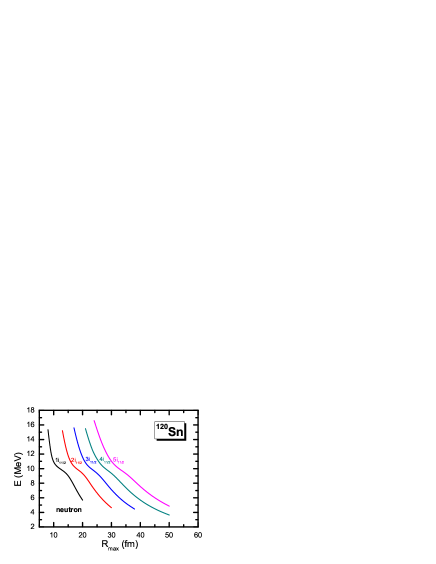
Figure 5: Positive energy $\nu$i_11/2 states in ¹²⁰Sn under different box boundary conditions.

Figure 6: The radial wave function for the neutron $\nu$i_11/2 resonant state in ¹²⁰Sn.

Except the state $\nu$i_13/2, there is another neutron resonant state with $l=6$, i.e., the $\nu$i_11/2 state. As shown in Fig. 5, there is a less stable state lying at about 10 MeV. Although it shares the same centrifugal barrier with $\nu$i_13/2, $\nu$i_11/2 is much wider because its energy is much larger than that of $\nu$i_13/2. In Fig. 6, one finds also that the wave function of $\nu$i_13/2 oscillates very much even at $r=50$ fm. The resonance parameters for this state are $E_{\gamma}=9.811$ MeV and $\Gamma=1.275$ MeV respectively.

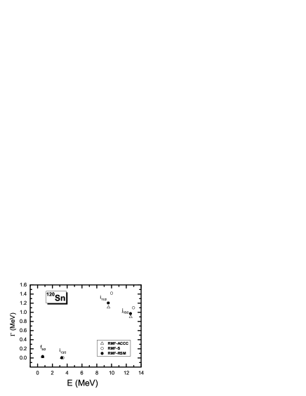
Figure 7: Energies and widths of single neutron resonant states in ¹²⁰Sn from different methods. RMF-ACCC, RMF-RSM, and RMF-S represents results from the analytical continuation in the coupling constant approach, the real stabilization method, and the scattering phase shift method in the framework of the RMF model with NL3 parameter set.

Table 2: Energies and widths of single neutron resonant states in ¹²⁰Sn from different methods. RMF-ACCC, RMF-RSM, and RMF-S represents results from the analytical continuation in the coupling constant approach, the real stabilization method, and the scattering phase shift method in the framework of the RMF model. In the RMF-RSM calculations, both PK1 and NL3 parameter sets are used. All quantities are in MeV.

	RMF-RSM (PK1)		RMF-RSM (NL3)		RMF-ACCC (NL3)		RMF-S (NL3)
$\nu l_{j}$	$E_{\gamma}$	$\Gamma$	$E_{\gamma}$	$\Gamma$	$E_{\gamma}$	$\Gamma$	$E_{\gamma}$	$\Gamma$
$\nu$f5/2	0.870	0.064	0.674	0.030	0.685	0.023	0.688	0.032
$\nu$i13/2	3.469	0.005	3.266	0.004	3.262	0.004	3.416	0.005
$\nu$i11/2	9.811	1.275	9.559	1.205	9.60	1.11	10.01	1.42
$\nu$j15/2	12.865	1.027	12.564	0.973	12.60	0.90	12.97	1.10

The energies and widths of single particle neutron resonant states obtained from the RSM calculations are summarized in Table 2. We also calculate these resonances using the parameter set NL3 for the Lagrangian density in the RMF model and compare the present results with those from the ACCC approach and the scattering phase shift method Zhang04b in Table 2. In Fig. 7, the comparison is also made in a planar $E_{\gamma}$-$\Gamma$ plot. For the two low lying resonant states, $\nu$f_5/2 and $\nu$i_13/2, the three methods give consistent results both for the energy and the width. Although similar energies are obtained from these three models for higher resonances, $\nu$i_11/2 and $\nu$j_15/2, clear differences occur among the widths from the ACCC approach and the scattering method and the results from the RSM lies in between.

IV Summary

In summary, the real stabilization method (RSM) has been developed within the framework of the relativistic mean field (RMF) model. With the self-consistent nuclear potentials provided by the RMF calculations with the parameter sets PK1 and NL3 for the Lagrangian density, the Dirac equation for the neutron is solved in the coordinate space under the box boundary condition. By investigating the stable behavior of the positive energy states against changes of the box size, the resonant states are singled out. The RMF-RSM is used to study single neutron resonant states in spherical nuclei. As examples, the energies, widths and wave functions of low-lying neutron resonant states in ¹²⁰Sn are obtained. Since a very large box size is used, even wider resonances can also be found. These results are compared with those from the scattering phase shift method and the analytic continuation in the coupling constant method and satisfactory agreements are found.

- (1) A. Bulgac, Preprint FT-194-1980, Central Institute of Physics, Bucharest, 1980 [arXiv: nucl-th/9907088].
- (2) J. Dobaczewski, H. Flocard, and J. Treiner, Nucl. Phys. A422, 103 (1984).
- (3) J. Dobaczewski, W. Nazarewicz, T. R. Werner, J.-F. Berger, C. R. Chinn, and J. Dechargé, Phys. Rev. C 53, 2809 (1996).
- (4) J. Meng and P. Ring, Phys. Rev. Lett. 77, 3963 (1996).
- (5) W. Pöschl, D. Vretenar, G. A. Lalazissis, and P. Ring, Phys. Rev. Lett. 79, 3841 (1997).
- (6) J. Meng, Nucl. Phys. A635, 3 (1998).
- (7) P. Curutchet, T. Vertse and R. J. Liotta, Phys. Rev. C. 39, 1020 (1989).
- (8) L. G. Cao, Z. Y. Ma, Phys. Rev. C. 66, 024311 (2002).
- (9) Kiyoshi Kato, J. Phys.: Conf. Ser. 49, 73 (2006).
- (10) A. T. Kruppa, R. G. Lovas, and B. Gyarmati, Phys. Rev. C 37, 383 (1988).
- (11) W. P. Reinhardt, Ann. Rev. Phys. Chem. 33, 223 (1982).
- (12) Y. K. Ho, Phys. Rep. 99, 1 (1983).
- (13) N. Moiseyev, Phys. Rep. 302, 212 (1998).
- (14) B. Gyarmati and A. T. Kruppa, Phys. Rev. C 34 (1986) 95.
- (15) A. T. Kruppa, P. -H. Heenen, H. Flocard, and R. J. Liotta, Phys. Rev. Lett. 79, 2217 (1997).
- (16) K. Arai, Phys. Rev. C 74, 064311 (2006).
- (17) V. I. Kukulin and V. M. Krasnopol’sky, J. Phys. A 10, 33 (1977).
- (18) V. I. Kukulin, V. M. Krasnopol’sky, and M. Miselkhi, Sov. J. Nucl. Phys. 29, 421 (1979).
- (19) V. I. Kukulin, V. M. Krasnopl’sky, and J. Horácek, Thoery of Resonances: Principles and Applications (Kluwer Academic, Dordrecht, 1989).
- (20) N. Tanaka, Y. Suzuki, and K. Varga, Phys. Rev. C56, 562 (1997).
- (21) N. Tanaka, Y. Suzuki, K. Varga, and R. G. Lovas, Phys. Rev. C59, 1391 (1999).
- (22) S. C. Yang, J. Meng, S. G. Zhou, Chin. Phys. Lett. 18, 196 (2001).
- (23) G. Cattapan and E. Maglione, Phys. Rev. C61, 067301 (2000).
- (24) S. S. Zhang, J. Meng, S. G. Zhou, and G. C. Hillhouse, Phys. Rev. C 70, 034308 (2004).
- (25) A. U. Hazi, H. S. Taylor, Phys. Rev. A1, 1109 (1970).
- (26) C. H. Maier, L. S. Cederbaum and W. Domcke, J. Phys. B 13, L119 (1980).
- (27) M. F. Fels and A. U. Hazi, Phys. Rev. A4, 662 (1971).
- (28) M. F. Fels and A. U. Hazi, Phys. Rev. A5, 1236 (1972).
- (29) H. S. Taylor and A. U. Hazi, Phys. Rev. A14, 2071 (1976).
- (30) V. A. Mandelshtam, T. R. Ravuri, and H. S. Taylor, Phys. Rev. Lett. 70, 1932 (1993).
- (31) V. A. Mandelshtam, H. S. Taylor, V. Ryaboy, and N. Moiseyev, Phys. Rev. A 50, 2764 (1994).
- (32) A. T. Kruppa and K. Arai, Phys. Rev. A 59, 3556 (1999).
- (33) B. D. Serot and J. D. Walecka, Adv. Nucl. Phys. 16, 1 (1986).
- (34) P.-G. Reinhard, Rep. Prog. Phys. 52, 439 (1989).
- (35) P. Ring, Prog. Part. Nucl. Phys. 37, 193 (1996).
- (36) D. Vretenar, A.V. Afanasjev, G.A. Lalazissis and P. Ring, Phys. Rep. 409, 101 (2005).
- (37) J. Meng, H. Toki, S.-G. Zhou, S. Q. Zhang, W. H. Long, and L. S. Geng, Prog. Part. Nucl. Phys. 57, 470 (2006).
- (38) J. Boguta and A. R. Bodmer, Nucl. Phys. A 292, 413 (1977).
- (39) C. J. Horowitz and B. D. Serot, Nucl. Phys. A368, 503 (1981).
- (40) Y. K. Gambhir, P. Ring and A. Thimet, Ann. Phys. (NY) 198, 132 (1990).
- (41) L. Zhang, S. G. Zhou, J. Meng and E. G. Zhao, Acta Physica Sinica 56, 3839 (2007) (in Chinese).
- (42) W. Long, J. Meng, N. Van Giai, and S. G. Zhou, Phys. Rev. C 69, 034319 (2004).
- (43) G. A. Lalazissis, J. König, and P. Ring, Phys. Rev. C 55, 540 (1997).
- (44) N. Sandulescu, L. S. Geng, H. Toki, and G. C. Hillhouse, Phys. Rev. C 68, 054323 (2003).
- (45) S. S. Zhang, Ph. D. thesis, Peking Univeristy, 2004 (in Chinese).