Analytic continuation of single-particle resonance energy and wave function in relativistic mean field theory

Single-particle resonant states in spherical nuclei are studied by an analytic continuation in the coupling constant (ACCC) method within the framework of the self-consistent relativistic mean field (RMF) theory. Taking the neutron resonant state $\nu 1g_{9/2}$ in ⁶⁰Ca as an example, we examine the analyticity of the eigenvalue and eigenfunction for the Dirac equation with respect to the coupling constant by means of a Pad$\acute{\text{e}}$ approximant of the second kind. The RMF-ACCC approach is then applied to ¹²²Zr and, for the first time, this approach is employed to investigate both the energies, widths and wave functions for $l\neq 0$ resonant states close to the continuum threshold. Predictions are also compared with corresponding results obtained from the scattering phase shift method.

I Introduction

The physics of exotic nuclei with unusual $N/Z$ ratios (isospin) has attracted world-wide attention. These nuclei are usually loosely bound and often exhibit resonances with a pronounced single-particle character since the Fermi surface approaches the continuum. In some nuclei, the valence nucleons can be easily scattered into single-particle resonant states (or Gamow states) in the continuum which is essential for the existence of exotic phenomena. For example, the halo in ¹¹Li TA85 can be successfully reproduced MR96 and giant halo nuclei MR98 are predicted by the relativistic continuum Hartree-Bogoliubov (RCHB) theory ME98 in which the contribution from the continuum has been proven to be crucial to understand these halo phenomena. There are also other attempts to include the contribution from the continuum in the non-relativistic San00 and relativistic approaches San . By taking into account a few resonant states close to the continuum threshold with the BCS method San , the relativistic mean field (RMF) theory seems to be able to reproduce the RCHB results and describe the main effects of the continuum. It has also been shown that the contribution of the continuum to the giant resonances mainly comes from Gamow states Curutchet89 ; Cao02 . Therefore, a proper treatment of resonant states is important for a deeper understanding of the properties in exotic nuclei.

Presently, several techniques have been developed to study resonant states in the continuum. One of them is the R-matrix theory in which resonance parameters (i.e. energy and width) can be reasonably determined from fitting the available experimental data Wigner47 . The extended R-matrix theory Hale87 and the K-matrix theory Humblet91 have also been developed. The conventional scattering theory is also an efficient tool for studying resonances. More precisely, the phase shift method is commonly used to determine parameters for a resonant state which corresponds to a pole of the S matrix Taylor72 . By discretizing the continuum, the contribution of the resonant states can be self-consistently taken into account via a Bogoliubov transformation in coordinate space Dobaczewski84 ; MR96 .

Computationally, it is desired to deduce the properties of unbound states from the eigenvalues and eigenfunctions of Hamiltonians for bound states so that the methods developed for bound states can still be used. For this purpose, the bound-state-type methods have been developed, including the real stabilization method Hazi70 , the complex scaling method (CSM) Ho83 , and the analytic continuation in the coupling constant (ACCC) method kukulin89 . In the real stabilization method, the continuum is discretized in a box and the resonance can be found according to the fact that its energy should be stable against the change of the box size. Sometimes it is difficult to find the appropriate box sizes, and it also turns out that this approach is suitable for narrow resonances only tanaka99 . In the CSM, the wave function for a resonant state is transformed to the square-integrable wave function for a bound state by rotating the position vector in coordinate space into the complex plane. Since the CSM involves the calculations of complex matrix elements, the corresponding difficulties related to complex eigenvalue problem still exist. In the ACCC method, a resonant state becomes a bound state if one increases the attractive potential and the energy, width and wave function for the resonant state can be obtained by an analytic continuation carried out via a Pad$\acute{\text{e}}$ approximant (PA) from the bound-state solutions. Compared with other bound-state-type methods, the ACCC approach is very effective and numerically quite simple because many methods available for bound-state problems can be used and the PA for analytic continuation can be implemented easily.

Within the framework of the non-relativistic Schrödinger equation, the ACCC method has been applied to investigate the energies and widths for resonant states in light nuclei combined with few-body methods tanaka99 ; Aoyama02 , and to study single-particle resonant states in spherical and deformed nuclei by solving the Schrödinger equation with Woods-Saxon potentials cattapan . Based on the Schrödinger and Dirac equations, the stability and convergence of the energies and widths for single-particle resonant states with square-well, harmonic-oscillator and Woods-Saxon potentials have been investigated and their dependence on the coupling constant interval and the order of the PA have been discussed in detail ZhangSch ; ZhangDirac .

The relativistic mean field (RMF) theory is widely used to describe properties of nuclear matter and finite nuclei successfully, not only for those nuclei near the valley of stability, but also for exotic nuclei with large neutron (proton) excess Ring96 ; MR96 . Previously the ACCC method was employed to study energies and widths for resonant states in stable nuclei ¹⁶O and ⁴⁸Ca in RMF theory Yang01 . In the present work, we aim at exploring the single-particle resonant states, including resonance parameters and wave functions, in exotic nuclei by the ACCC method within the framework of the RMF theory. This paper represents the first application of the RMF-ACCC method to obtain both the wave functions and resonance parameters. The paper is organized as follows. In Sec. II the ACCC method combined with the RMF theory is presented. The numerical details are given in Sec. III and its application to the doubly magic nucleus ¹²²Zr in Sec. IV. Finally, we give a brief summary in Sec. V.

II Theoretical framework

II.1 Relativistic Mean Field Theory

The basic ansatz of the RMF theory is a Lagrangian density whereby nucleons are described as Dirac particles which interact via the exchange of various mesons (the scalar $\sigma$, vector $\omega$ and iso-vector vector $\rho$) and the photon ME98

$$\begin{array}[]{cc}{\cal L}&=\bar{\psi}(i\hbox to0.0pt{/\hss}\partial-M)\psi+\,{1\over 2}\partial_{\mu}\sigma\partial^{\mu}\sigma-U(\sigma)-{1\over 4}\Omega_{\mu\nu}\Omega^{\mu\nu}\\ &+{1\over 2}m_{\omega}^{2}\omega_{\mu}\omega^{\mu}-{1\over 4}{{\mbox{\boldmath${\rm R}$}}}_{\mu\nu}{{\mbox{\boldmath${\rm R}$}}}^{\mu\nu}+{1\over 2}m_{\rho}^{2}{\mbox{\boldmath${\rm\rho}$}}_{\mu}{\mbox{\boldmath${\rm\rho}$}}^{\mu}-{1\over 4}F_{\mu\nu}F^{\mu\nu}\\ &-g_{\sigma}\bar{\psi}\sigma\psi~{}-~{}g_{\omega}\bar{\psi}\hbox to0.0pt{/\hss}\omega\psi~{}-~{}g_{\rho}\bar{\psi}\hbox to0.0pt{/\hss}{\mbox{\boldmath${\rm\rho}$}}{\mbox{\boldmath${\rm\tau}$}}\psi-~{}e\bar{\psi}\hbox to0.0pt{/\hss}{\mbox{\boldmath${\rm A}$}}\psi,\end{array}$$ (4)

where $M$ is the nucleon mass and $m_{\sigma}$ ($g_{\sigma}$), $m_{\omega}$ ($g_{\omega}$), and $m_{\rho}$ ($g_{\rho}$) are the masses (coupling constants) of the respective mesons. A nonlinear scalar self-interaction $U(\sigma)~{}=~{}\dfrac{1}{2}m^{2}_{\sigma}\sigma^{2}~{}+~{}\dfrac{g_{2}}{3}\sigma^{3}~{}+~{}\dfrac{g_{3}}{4}\sigma^{4}$ of the $\sigma$ meson has been included BB77 . The field tensors for the vector mesons are given as

$$\left\{\begin{array}[]{lll}\Omega^{\mu\nu}&=&\partial^{\mu}\omega^{\nu}-\partial^{\nu}\omega^{\mu},\\ {{\mbox{\boldmath${\rm R}$}}}^{\mu\nu}&=&\partial^{\mu}{{\mbox{\boldmath${\rm\rho}$}}}^{\nu}-\partial^{\nu}{{\mbox{\boldmath${\rm\rho}$}}}^{\mu}-g^{\rho}({{\mbox{\boldmath${\rm\rho}$}}}^{\mu}\times{{\mbox{\boldmath${\rm\rho}$}}}^{\nu}),\\ F^{\mu\nu}&=&\partial^{\mu}{\mbox{\boldmath${\rm A}$}}^{\nu}-\partial^{\nu}{\mbox{\boldmath${\rm A}$}}^{\mu}.\end{array}\right.$$ (8)

The classical variation principle gives the following equations of motion

$$[{{\mbox{\boldmath${\rm\alpha}$}}}\cdot{{\mbox{\boldmath${\rm p}$}}}+V_{V}({{\mbox{\boldmath${\rm r}$}}})+\beta(M+V_{S}({{\mbox{\boldmath${\rm r}$}}}))]\psi_{i}~{}=~{}\epsilon_{i}\psi_{i},$$ (9)

for the nucleon spinors, where $\varepsilon_{i}$ and $\psi_{i}$ are the single-particle energy and spinor wave function respectively, and the Klein-Gordon equations

$$\left\{\begin{array}[]{lll}\left(-\Delta\sigma~{}+~{}U^{\prime}(\sigma)\right)&=&g_{\sigma}\rho_{s},\\ \left(-\Delta~{}+~{}m_{\omega}^{2}\right)\omega^{\mu}&=&g_{\omega}j^{\mu}({{\mbox{\boldmath${\rm r}$}}}),\\ \left(-\Delta~{}+~{}m_{\rho}^{2}\right){{\mbox{\boldmath${\rm\rho}$}}}^{\mu}&=&g_{\rho}{\mbox{\boldmath${\rm j}$}}^{\mu}({{\mbox{\boldmath${\rm r}$}}}),\\ -\Delta~{}A_{0}^{\mu}({{\mbox{\boldmath${\rm r}$}}}){}&=&ej_{\rho}^{\mu}({{\mbox{\boldmath${\rm r}$}}}),\end{array}\right.$$ (14)

for the mesons, where

$$\left\{\begin{array}[]{lll}V_{V}({{\mbox{\boldmath${\rm r}$}}})&=&g_{\omega}\hbox to0.0pt{/\hss}\omega+g_{\rho}\hbox to0.0pt{/\hss}{\mbox{\boldmath${\rm\rho}$}}{\mbox{\boldmath${\rm\tau}$}}+\dfrac{1}{2}e(1-\tau_{3})\hbox to0.0pt{\,/\hss}{\mbox{\boldmath${\rm A}$}},\\ V_{S}({{\mbox{\boldmath${\rm r}$}}})&=&g_{\sigma}\sigma,\\ \end{array}\right.$$ (17)

are the vector and scalar potentials respectively and the source terms for the mesons are

$$\left\{\begin{array}[]{lll}\rho_{s}&=&\sum\limits_{i=1}^{A}\bar{\psi}_{i}\psi_{i},\\ j^{\mu}({{\mbox{\boldmath${\rm r}$}}})&=&\sum\limits_{i=1}^{A}\bar{\psi}_{i}\gamma^{\mu}\psi_{i},\\ {\mbox{\boldmath${\rm j}$}}^{\mu}({{\mbox{\boldmath${\rm r}$}}})&=&\sum\limits_{i=1}^{A}\bar{\psi}_{i}\gamma^{\mu}{\mbox{\boldmath${\rm\tau}$}}\psi_{i},\\ j^{\mu}_{p}({{\mbox{\boldmath${\rm r}$}}})&=&\sum\limits_{i=1}^{A}\bar{\psi}_{i}\gamma^{\mu}\dfrac{1-\tau_{3}}{2}\psi_{i}.\end{array}\right.$$ (22)

It should be noted that the contribution of negative energy states are neglected, i.e., the vacuum is not polarized. Moreover, the mean field approximation is carried out via replacing meson field operators in Eq. (9) by their expectation values, since the coupled equations Eq. (9) and Eq. (14) are nonlinear quantum field equations and their exact solutions are very complicated. In this way, the nucleons are assumed to move independently in the classical meson fields. The coupled equations can be solved self-consistently by iteration.

For spherical nuclei, the potential of the nucleon and the sources of meson fields depend only on the radial coordinate $r$. The spinor is characterized by the angular momentum quantum numbers $l$, $j$, $m$, the isospin $t=\pm\dfrac{1}{2}$ for neutron and proton respectively, and the other quantum number $i$. The Dirac spinor has the form

$$\psi({\mbox{\boldmath${\rm r}$}})=\left({{\mbox{i}\dfrac{G_{i}^{lj}(r)}{r}{Y^{l}_{jm}(\theta,\phi)}}\atop{\dfrac{F_{i}^{lj}(r)}{r}({\mbox{\boldmath${\rm\sigma}$}}\cdot\hat{{\mbox{\boldmath${\rm r}$}}}){Y^{l}_{jm}(\theta,\phi)}}}\right)\chi_{t}(t),$$ (23)

where $Y^{l}_{jm}(\theta,\phi)$ are the spinor spherical harmonics. The radial equation of the spinor, i.e. Eq. (9), can be reduced to  ME98

$$(-\dfrac{\partial}{\partial r}+\dfrac{\kappa}{r})F_{i}^{lj}(r)+\left[M+V_{p}(r)\right]G_{i}^{lj}(r) = \varepsilon_{i}G_{i}^{lj}(r),$$

$$(\dfrac{\partial}{\partial r}+\dfrac{\kappa}{r})G_{i}^{lj}(r)-\left[M-V_{m}(r)\right]F_{i}^{lj}(r) = \varepsilon_{i}F_{i}^{lj}(r),$$ (24)

in which $V_{p}(r)=V_{V}(r)+V_{S}(r)$, $V_{m}(r)=V_{V}(r)-V_{S}(r)$, and $\kappa=(-1)^{j+l+1/2}(j+1/2)$. The meson field equations can be reduced to

$$\left(\frac{\partial^{2}}{\partial r^{2}}-\frac{2}{r}\frac{\partial}{\partial r}+m_{\phi}^{2}\right)\phi=s_{\phi}(r),$$ (25)

where $\phi=\sigma$, $\omega$, $\rho$, and photon ( $m_{\phi}=0$ for photon). The source terms read

$$s_{\phi}(r)=\left\{\begin{array}[]{ll}-g_{\sigma}\rho_{s}-g_{2}\sigma^{2}(r)-g_{3}\sigma^{3}(r)&{\rm for~{}the~{}\sigma~{}field},\\ g_{\omega}\rho_{v}&{\rm for~{}the~{}\omega~{}field},\\ g_{\rho}\rho_{3}(r)&{\rm for~{}the~{}\rho~{}field},\\ e\rho_{c}(r)&{\rm for~{}the~{}Coulomb~{}field},\\ \end{array}\right.$$ (30)

and

$$\left\{\begin{array}[]{lll}4\pi r^{2}\rho_{s}(r)&=&\sum\limits_{i=1}^{A}(|G_{i}(r)|^{2}-|F_{i}(r)|^{2}),\\ 4\pi r^{2}\rho_{v}(r)&=&\sum\limits_{i=1}^{A}(|G_{i}(r)|^{2}+|F_{i}(r)|^{2}),\\ 4\pi r^{2}\rho_{3}(r)&=&\sum\limits_{p=1}^{Z}(|G_{p}(r)|^{2}+|F_{p}(r)|^{2})-\sum\limits_{n=1}^{N}(|G_{n}(r)|^{2}+|F_{n}(r)|^{2}),\\ 4\pi r^{2}\rho_{c}(r)&=&\sum\limits_{p=1}^{Z}(|G_{p}(r)|^{2}+|F_{p}(r)|^{2}).\\ \end{array}\right.$$ (35)

II.2 Analytic Continuation in the Coupling Constant for Resonance Parameters and Gamow Wave Functions

By solving Eqs. (II.1) and (25) in a meshed box of size $R_{0}$ self-consistently, one can calculate the ground state properties of a nucleus. The vector potential $V_{V}(r)$ and the scalar potential $V_{S}(r)$, energies and wave functions for bound states are also obtained. By increasing the attractive potential as $V_{p}(r)\rightarrow\lambda V_{p}(r)$, a resonant state will be lowered and becomes a bound state if the coupling constant $\lambda$ is large enough. Near the branch point $\lambda_{0}$, defined by the scattering threshold $k(\lambda_{0})=0$ kukulin89 , the wave number $k(\lambda)$ behaves as

$$k(\lambda)\sim\left\{\begin{array}[]{l@{\mbox{~~~}}l}i\sqrt{\lambda-\lambda_{0}},\hfil\mbox{~{}~{}~{}&l>0,\\ i(\lambda-\lambda_{0}),\hfil\mbox{~{}~{}~{}&l=0.\end{array}\right.}}$$ (38)

These properties suggest an analytic continuation of the wave number $k$ in the complex $\lambda$ plane from the bound-state region into the resonance region by Pad$\acute{\text{e}}$ approximant of the second kind (PAII) kukulin89

$$k(x)\approx k^{[L,N]}(x)=i\dfrac{c_{0}+c_{1}x+c_{2}x^{2}+\ldots+c_{L}x^{L}}{1+d_{1}x+d_{2}x^{2}+\ldots+d_{N}x^{N}},$$ (39)

where $x\equiv\sqrt{\lambda-\lambda_{0}}$, and $c_{0},c_{1},\ldots,c_{L},d_{1},d_{2},\ldots,d_{N}$ are the coefficients of PA. These coefficients can be determined by a set of reference points $x_{i}$ and $k(x_{i})$ obtained from the Dirac equation with $\lambda_{i}>\lambda_{0},~{}i=1,2,...,L+N+1$. With the complex wave number $k(\lambda=1)=k_{r}+ik_{i}$, the resonance energy $E$ and the width $\Gamma$ can be extracted from the relation $\varepsilon=E-i\dfrac{\Gamma}{2}~{}~{}(E,\Gamma\in\mathbb{R})$ and $k^{2}=\varepsilon^{2}-M^{2}$, i.e.,

$$E = \sqrt{\dfrac{\sqrt{(M^{2}+k_{r}^{2}-k_{i}^{2})^{2}+4k_{r}^{2}k_{i}^{2}}+(M^{2}+k_{r}^{2}-k_{i}^{2})}{2}}-M,$$

$$\Gamma = \sqrt{2\sqrt{(M^{2}+k_{r}^{2}-k_{i}^{2})^{2}+4k_{r}^{2}k_{i}^{2}}-2(M^{2}+k_{r}^{2}-k_{i}^{2})}.$$ (40)

In the non-relativistic limit ($k\ll M$), Eq. (II.2) reduces to

$$E=\dfrac{k_{r}^{2}-k_{i}^{2}}{2M},~{}~{}~{}~{}~{}~{}~{}~{}~{}~{}~{}~{}~{}~{}~{}~{}~{}\Gamma=\dfrac{2k_{r}k_{i}}{M}.$$ (41)

It is evident that the continuation in the coupling constant can be replaced by the continuation in $k$ plane along the $k(\lambda)$ trajectory determined by Eq. (39) to the point $k_{R}$ corresponding to the wave number for Gamow state, i.e., $k_{R}=k^{[L,N]}(\lambda=1)$ kukulin89 . Similarly, the wave function $\varphi(k_{R},r)$ for a resonant state can be obtained by an analytic continuation of the bound-state wave function $\varphi(k_{i},r)$ in the complex $k$ plane. One can also prove that the wave function $\varphi(k,r)$ is an analytic function of the wave number $k$ in the inner region $r<R_{0}$ where the Jost function analyticity dominates kukulin89 . Therefore, we use the technique, which has been adopted to find the complex resonance energy, to determine the resonance wave function $\varphi(k_{R},r)$. Firstly, we construct the PA to define the resonance wave function at any point $r$ in the inner region ($r<R_{0}$) kukulin89

$$\varphi^{[L,N]}(k,r)=\dfrac{P_{L}(k,r)}{Q_{N}(k,r)}=\dfrac{a_{0}(r)+a_{1}(r)k+a_{2}(r)k^{2}+\ldots+a_{L}(r)k^{L}}{1+b_{1}(r)k+b_{2}(r)k^{2}+\ldots+b_{N}(r)k^{N}},$$ (42)

where the coefficients ${a_{i}(r)}~{}(i=0,1,\ldots,L)$ and ${b_{j}(r)}~{}(j=1,2,\ldots,N)$ are dependent on $r$. These coefficients can be determined by a set of reference points $k_{i}$ and $\varphi(k_{i},r)$ obtained from the Dirac equation with $\lambda_{i}>\lambda_{0},~{}(i=1,2,...,L+N+1)$. The resonance wave function $\varphi(k_{R},r)=\varphi^{[L,N]}(k_{R},r)~{}(r<R_{0})$ can be extrapolated in this way.

Eq. (II.1) can be rewritten as two decoupled Schrödinger-like equations for the upper and the lower components respectively ME99 . For neutrons, the Schrödinger-like equation for the upper component reads

$$\dfrac{\partial^{2}G_{i}^{lj}(r)}{\partial r^{2}}-\dfrac{\kappa_{i}(\kappa_{i}+1)}{r^{2}}G_{i}^{lj}(r)+(\varepsilon_{i}^{2}-M^{2})G_{i}^{lj}(r)=0,$$ (43)

in the outer region where $V_{V}(r)\simeq 0$ and $V_{S}(r)\simeq 0$. Its solution is the well known Riccati-Hankel function

$$\hat{h}^{\pm}_{\kappa}(z)=\hat{n}_{\kappa}(z)\pm i\hat{j}_{\kappa}(z),~{}~{}~{}~{}~{}z=kr,$$ (44)

where $\hat{j}_{\kappa}(z)=z{j}_{\kappa}(z)$ is the usual regular solution, i.e. Riccati-Bessel function, and $\hat{n}_{\kappa}(z)=z{n}_{\kappa}(z)$ is the irregular solution, i.e. Riccati-Neumann function. The outer wave function is matched to the inner wave function at $r=r_{m}<R_{0}$

$$\varphi^{[L,N]}(k_{R},r_{m})=C(k_{R})\left[\hat{j}_{\kappa}(k_{R}r_{m})+D(k_{R})\hat{n}_{\kappa}(k_{R}r_{m})\right],$$ (45)

where $C(k_{R})$ is the coefficient for matching and $D(k_{R})=\tan\delta_{\kappa}(k_{R})$ with $\delta_{\kappa}(k_{R})$ the phase shift. It has been found that $\delta_{\kappa}(k_{R})$ is almost a constant when $r_{m}$ is large enough. Given the upper component, the lower component $F_{\kappa}(r)$ can be calculated from the relationship between the upper and the lower components derived from Eq. (II.1), i.e.,

$$F_{\kappa}(r)=\dfrac{(\varepsilon-m)}{k_{R}C(k_{R})}\left[\hat{j}_{\kappa-1}(k_{R}r)+D(k_{R})\hat{n}_{\kappa-1}(k_{R}r)\right].$$ (46)

Finally, the resonance wave function is normalized according to the Zel’dovich procedures kukulin89 .

III Numerical details

In this section we give the details on how the ACCC method is realized within the framework of the RMF theory and exploit the analyticity of the eigenvalues and eigenfunctions of the Dirac equation with respect to the coupling constant. In RCHB calculations ⁶⁰Ca is the doorway for exotic phenomena such as giant halos MR98 , in which the neutron resonant states play an important role in the continuum. We select the neutron resonant state $\nu 1g_{9/2}$ in ⁶⁰Ca to investigate the analyticity of the eigenvalue and eigenfunction for the Dirac equation with respect to the coupling constant. The RMF equations are solved in a spherical box of the size $R_{0}=20$ fm, with a mesh size of $\delta r=0.05$ fm ZMR03 . Several well used effective interactions for the RMF Lagrangian will be used and the corresponding results will be compared. The energy, width and wave function for the $\nu 1g_{9/2}$ resonant state in ⁶⁰Ca are obtained with the procedure given in the last section. As the stability and convergence (e.g., the dependence on PA order) of the energies and widths in the Dirac and Schrödinger equations have been investigated in Refs. ZhangSch ; ZhangDirac , we do not discuss them here and use $L=N=4$ PA for the present calculations.

In Tab. 1, we present the energies and widths for $\nu 1g_{9/2}$ in ⁶⁰Ca calculated with effective interactions NL3 NL3 , NLSH NLSH , TMA TMA and the newly developed PK1 PK1 parametrization. The results from the scattering phase shift method (RMF-S) obtained similarly as in Ref. San are also included for comparison. The first step in RMF-S is to solve the Dirac equation [Eq. (II.1)] with scattering boundary conditions for the continuum spectrum. The solutions, upper and lower components, have the same form as here in Eq. (45) and Eq. (46) respectively. The coefficients $C$ and $D$ in Eq. (45) and Eq. (46) are fixed by the normalization condition of the scattering wave functions and the phase shift $\delta$ is calculated from the matching conditions. It should be mentioned that the energy used in the wave functions is real and not unique, as opposed to complex and the unique value which is determined by the ACCC method in advance. In the vicinity of an isolated resonance, the resonance energy and width are extracted from the derivative of the phase shift $\delta$ in Breit-Wigner form, i.e.,

$$\dfrac{d\delta(E)}{dE}=\dfrac{\Gamma/2}{(E_{r}-E)^{2}+\Gamma^{2}/4}.$$ (47)

After discretizing the real energy for scattering solutions and phase shift variation, the resonance energy is uniquely determined.

One can find from Tab. 1 that the results from the ACCC and the scattering methods agree well. Different effective interactions give similar energies and widths. Therefore in the following calculations, we use only the effective interaction NL3 for illustration.

The resonance energy $E$ and width $\Gamma$ for the neutron resonant state $\nu 1g_{9/2}$ in ⁶⁰Ca, as a function of the coupling constant $\lambda$, are exhibited in Fig. 1. Filled circles and crosses are the solutions of the Dirac equation [Eq. (II.1)], and the former is used as input in the ACCC method. Solid curves are the outcome of $L=N=4$ PA [Eq. (39)]. The dashed vertical line corresponds to the branch point $\lambda_{0}>1$. When $\lambda>\lambda_{0}$, the particle is bound. With $\lambda$ decreasing from $\lambda_{0}$ down to 1, a nonvanishing imaginary part appears in the complex energy expressed by Eq. (II.2). At $\lambda=1$, one gets the resonance energy $E$ and width $\Gamma$. The agreement between the exact solutions of the Dirac equation with large coupling constant (crosses in Fig. 1) and the extrapolated results of PA (solid energy curve) is quite good, which demonstrates the validity of the ACCC method. The smooth solid line indicates good analyticity of the eigenvalue for the Dirac equation with respect to the coupling constant. The same results can also be obtained for the case of $L=N=5$ and $L=N=6$ PAs, similar as in Ref. ZhangSch ; ZhangDirac .

In Fig. 2, we show the real and imaginary parts of the upper component $G(r)$ and the lower component $F(r)$ at $r=5$ fm and $r=10$ fm respectively as functions of the resonance energy $E$ (which corresponds to the coupling constant $\lambda$ displayed in Fig. 1). Symbols in Fig. 2 have the same meaning as those in Fig. 1. The neutron feels much stronger effect from the nuclear potential at $r=5$ fm than at $r=10$ fm. Similar to the case of the eigenvalue discussed above, the real and the imaginary part of each component behave smoothly, which indicates good analyticity of the eigenfunction for the Dirac equation with respect to the coupling constant.

The wave function obtained from the analytic continuation is connected continuously to the free wave function at the matching point $r_{m}$. On one hand, the matching point $r_{m}$ should be large enough to make sure that the potential at $r_{m}$ vanishes, which is required by the outer part of the wave function. On the other hand, $r_{m}$ should be far enough from the box radius $R_{0}$ to guarantee that the inner part of the wave function can be obtained accurately. In the lower panel of Fig. 3, the potential $V_{V}(r)+V_{S}(r)$ for ⁶⁰Ca is plotted. One finds that when $r>14$ fm, the potential becomes smaller than $10^{-4}$ MeV which is good enough for the precision in our calculations. The upper limit of the matching point $r_{m}$ can be estimated by the behavior of the density from the upper panel in Fig. 3. The neutron density $\rho_{n}(r)$ in ⁶⁰Ca and $\rho_{\nu 1g_{9/2}}(r)\equiv[|G(r)|^{2}+|F(r)|^{2}]/4\pi r^{2}$ decline rapidly in the vicinity of 20 fm because of the boundary condition in the RMF calculation. The density curves in the range $r<18$ fm are smooth and behave reasonably. Therefore, the matching point should be chosen at any point between 14 fm and 18 fm. We present the wave function for the neutron resonant state $\nu 1g_{9/2}$ in ⁶⁰Ca with different matching points in Fig. 4. As expected, the wave function is the same when changing the matching point $r_{m}$ from 14 fm to 18 fm. In the following calculations, the wave function will be matched at $r_{m}=18$ fm, unless otherwise specified.

IV Application to single-particle resonant states in ¹²²Zr

We apply the ACCC method within the framework of the RMF theory to calculate the energies, widths and wave functions for the resonant states in ¹²²Zr. Since ¹²²Zr is the core of the giant neutron halo predicted in RCHB calculations MR98 , and the resonant states in ¹²²Zr have been obtained by the scattering method San , we choose this nucleus for comparison.

In Fig. 5, the energies and widths for the resonant states $\nu 3p_{3/2}$, $\nu 3p_{1/2}$, $\nu 2f_{7/2}$, $\nu 2f_{5/2}$, $\nu 1h_{9/2}$ and $\nu 1i_{13/2}$ are presented as a planar $E$–$\Gamma$ plot. The results of the ACCC and the scattering methods are in good agreement with each other for most of these states. From both methods, $\nu 2f_{5/2}$ and $\nu 1i_{13/2}$ have large widths, while $\nu 2f_{7/2}$ and $\nu 1h_{9/2}$ are very narrow. The width for $\nu 3p_{3/2}$ from the scattering method is slightly larger than our calculation. As for the resonant state $\nu 3p_{1/2}$, neither the energy nor the width can be extracted from the scattering calculation. From a quantum mechanical point of view, these single-particle resonant states are quasi-stationary ones captured by centrifugal barriers. The decay width for a resonant state can be roughly explained by the penetration through the barrier. For those states with the same $l$, i.e., the same centrifugal barrier, the higher state has a larger width, e.g., for the two $f$ states $\nu 2f_{5/2}$ and $\nu 2f_{7/2}$. Although $\nu 1h_{9/2}$ is higher than $\nu 2f_{5/2}$, its width is smaller because of higher centrifugal barrier. A similar argument also holds for a much higher but narrow state $\nu 1i_{13/2}$.

The wave functions for the resonant states $\nu 3p_{3/2}$, $\nu 2f_{7/2}$, $\nu 2f_{5/2}$ and $\nu 1h_{9/2}$ are respectively exhibited in Figs. 6, 7, 8, and 9. Since the imaginary part of the wave function is neglected in the scattering calculations San ; San00 , only the real parts of the upper and the lower components are given and compared in these figures. In Fig. 6, one finds a considerable difference for the upper components at large $r$ in $\nu 3p_{3/2}$ between these two methods. This difference is consistent with the difference in energy and width as seen in Fig. 5. A similar difference is also seen for $\nu 2f_{5/2}$ in Fig. 8. For those states where the two methods give nearly the same energies and widths, e.g., $\nu 2f_{7/2}$ and $\nu 1h_{9/2}$, the wave functions agree quite well. The small difference for the wave functions between these two methods found in Figs. 7 and 9 might be from the neglect of the imaginary part of the wave function in the scattering method.

V Summary

In summary, the method of the analytic continuation in the coupling constant (ACCC) has been developed within the framework of the relativistic mean field (RMF) theory and used to investigate the resonance energies, widths and wave functions for single-particle resonant states in exotic nuclei. The analyticity of these quantities, as functions of the coupling constant, are exploited for the neutron resonant state $\nu 1g_{9/2}$ in ⁶⁰Ca. The energies, widths and wave functions for some resonant states in ¹²²Zr are calculated and compared with those obtained from the scattering method. The results from the ACCC method agrees satisfactorily with those from the scattering calculation as well as available data  Yang01 . It is expected that the RMF-ACCC method, combined with the BCS theory, can be generalized to describe exotic phenomena in unstable nuclei.

Tab. 1: Energies and widths ($E,~{}\Gamma)$ in MeV for the neutron resonant state $\nu 1g_{9/2}$ in ⁶⁰Ca calculated by the ACCC (RMF-ACCC) and the scattering (RMF-S) method with the effective interactions NL3, NLSH, PK1, and TMA.

	NL3	NLSH	PK1	TMA
RMF-ACCC [MeV]	(0.49, 0.0005)	(0.47, 0.0004)	(0.77, 0.0009)	(0.77, 0.0009)
RMF-S [MeV]	(0.54, 0.0001)	(0.53, 0.0001)	(0.85, 0.0006)	(0.83, 0.0005)

Fig. 1: Energy $E$ and width $\Gamma$ for the neutron resonant state $\nu 1g_{9/2}$ in ⁶⁰Ca, as a function of the coupling constant $\lambda$. Filled circles and crosses are the solutions of the Dirac equation, and the former is used as input in the ACCC method. Solid curves are the outcome of $L=N=4$ PA.

Fig. 2: The real and imaginary part of the upper component $G(r)$ and the lower component $F(r)$ for the neutron $\nu 1g_{9/2}$ state in ⁶⁰Ca at (a) $r=5$ fm and (b) $r=10$ fm as functions of the resonance energy $E$ (which corresponds to the coupling constant $\lambda$ displayed in Fig. 1). Symbols have the same meaning as those in Fig. 1.

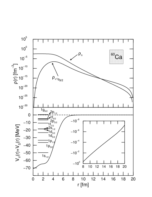
Fig. 3: Neutron densities for ⁶⁰Ca and for the neutron $\nu 1g_{9/2}$ state (upper panel); the potential $V_{V}(r)+V_{S}(r)$, the single-particle neutron bound states and the neutron resonant state $\nu 1g_{9/2}$ (lower panel).

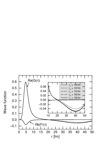
Fig. 4: Real parts of the upper and lower components of the radial wave function for the neutron $\nu 1g_{9/2}$ state in ⁶⁰Ca calculated by the ACCC method with different matching points $r_{m}$.

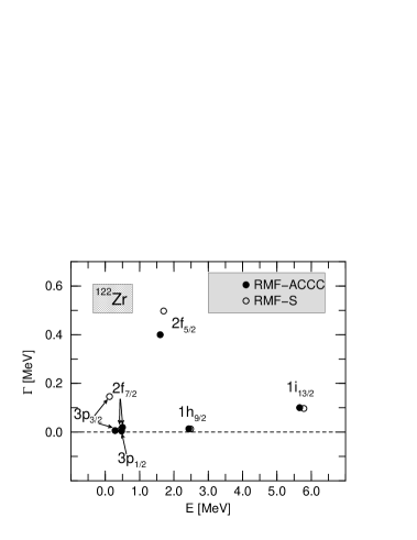
Fig. 5: Energies and widths for the neutron state $\nu 3p_{3/2}$, $\nu 3p_{1/2}$, $\nu 2f_{7/2}$, $\nu 2f_{5/2}$, $\nu 1h_{9/2}$, and $\nu 1i_{13/2}$ in ¹²²Zr. Solid circles represent the results of the ACCC method, while open circles denote the results of the scattering method.

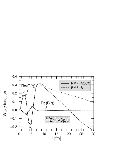
Fig. 6: Real parts of the upper and lower components of radial wave functions for the neutron resonant state $\nu 3p_{3/2}$ in ¹²²Zr. Solid and dashed curves represent the results of the ACCC and the scattering method respectively.

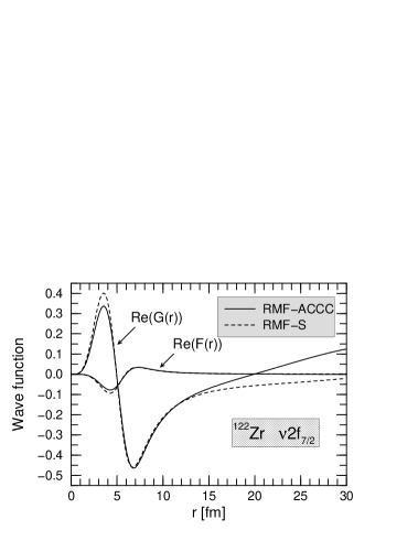
Fig. 7: Similar as Fig. 6, but for the neutron resonant state $\nu 2f_{7/2}$ in ¹²²Zr.

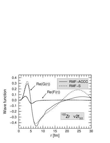
Fig. 8: Similar as Fig. 6, but for the neutron resonant state $\nu 2f_{5/2}$ in ¹²²Zr.

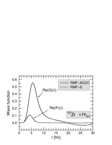
Fig. 9: Similar as Fig. 6, but for the neutron resonant state $\nu 1h_{9/2}$ in ¹²²Zr.