Reducing the Tension Between the BICEP2 and the Planck Measurements:
A Complete Exploration of the Parameter Space

Abstract

A large inflationary tensor-to-scalar ratio $r_{\mathrm{0.002}}=0.20^{+0.07}_{-0.05}$ is reported by the BICEP2 team based on their B-mode polarization detection, which is outside of the $95\%$ confidence level of the Planck best fit model. We explore several possible ways to reduce the tension between the two by considering a model in which $\alpha_{\mathrm{s}}$, $n_{\mathrm{t}}$, $n_{\mathrm{s}}$ and the neutrino parameters $N_{\mathrm{eff}}$ and $\Sigma m_{\mathrm{\nu}}$ are set as free parameters. Using the Markov Chain Monte Carlo (MCMC) technique to survey the complete parameter space with and without the BICEP2 data, we find that the resulting constraints on $r_{\mathrm{0.002}}$ are consistent with each other and the apparent tension seems to be relaxed. Further detailed investigations on those fittings suggest that $N_{\mathrm{eff}}$ probably plays the most important role in reducing the tension. We also find that the results obtained from fitting without adopting the consistency relation do not deviate much from the consistency relation. With available Planck, WMAP, BICEP2 and BAO datasets all together, we obtain $r_{0.002}=0.14_{-0.11}^{+0.05}$, $n_{\mathrm{t}}=0.35_{-0.47}^{+0.28}$, $n_{\mathrm{s}}=0.98_{-0.02}^{+0.02}$, and $\alpha_{\mathrm{s}}=-0.0086_{-0.0189}^{+0.0148}$; if the consistency relation is adopted, we get $r_{0.002}=0.22_{-0.06}^{+0.05}$.

1 Introduction

The BICEP2 experiment[1, 2], a dedicated cosmic microwave background (CMB) polarization experiment, has announced recently the detection of the B-mode polarization in CMB, based on an observation of about 380 square degrees low-foreground area of sky during 2010 to 2012 in the South Pole. The detected B-mode power is in the multipole range $30<\ell<150$. Because the CMB lensing peaks at $\ell\sim 1000$, the excess of B-mode power at these small $\ell\sim 100$s can not be explained by the lensing contribution, which is too small. It has been pointed out in that the foreground residual from Galactic dust may contribute to B-mode power [3, 4, 5]. The BICEP2 team has examined possible systematic errors and potential foreground contaminations, and found that the cross-correlations between frequency bands have little changes in the observed amplitude, which imply that frequency-dependent foreground may not be the dominant contributor. If the CMB polarization B-modes observed by BICEP2 is confirmed, it would indicate the presence of tensor perturbations, i.e. gravitational waves in the early universe, and provide a strong evidence of the inflationary origin of the universe.

The inflation theory which has been developed since the 1980s solves a number of cosmological conundrums, like the monopole, horizon, smoothness, and entropy problems [6, 7, 8, 9]. The quantum fluctuations streched by the inflationary expansion, give rise the scalar and tensor primordial power spectrum. Considering the $\Lambda$CDM model and assuming the scalar perturbation are purely adiabatic, it is convenient to expand the scalar and tensor power spectrum as

$$P_{\mathrm{\zeta}}\left(k\right) \equiv A_{\mathrm{s}}\left(\frac{k}{k_{0}}\right)^{n_{\mathrm{s}}-1+\frac{1}{2}\alpha_{\mathrm{s}}\ln\frac{k}{k_{0}}}\mathrm{,}\;\;$$ (1)

$$P_{\mathrm{t}}\left(k\right) \equiv A_{\mathrm{t}}\left(\frac{k}{k_{0}}\right)^{n_{\mathrm{t}}}\mathrm{,}\;\;$$ (2)

where $k_{0}$ is the pivot scale, it is usually chosen to be $0.05$ Mpc^-1, roughly in the middle of the logarithmic range of scales probed by WMAP and Planck experiments; $A_{\mathrm{s}}$, $n_{\mathrm{s}}$ are the amplitude and spectral index for the scalar power spectrum respectively, while $A_{\mathrm{t}}$, $n_{\mathrm{t}}$ are for the tensor power spectrum respectively; $\alpha_{\mathrm{s}}$ denotes the running of the scalar spectrum tilt[10] with $\alpha_{\mathrm{s}}=\frac{d\,n_{\mathrm{s}}}{d\,{\rm ln}\,k}$. An important parameter, the tensor-to-scalar ratio, which indicates the ratio of the tensor power to the scalar power, is defined as

$$r=\frac{P_{\zeta}(k)}{P_{t}(k)}\mathrm{,}$$ (3)

$r$ can be scale dependent, and the single field slow-roll inflation implies a tensor-to-scalar ratio of $r_{0.05}=-8n_{\mathrm{t}}$, in which the subscript $0.05$ indicates the particular pivot scale of $k=0.05$ Mpc^-1. This relation is referred as the consistency relation.

The BICEP2 team reported their measured value of tensor-to-scalar ratio, at scale $k=0.002$ Mpc^-1, as $r_{0.002}=0.20^{+0.07}_{-0.05}$, based on the lensed-$\Lambda$CDM+tensor model. The result is derived from importance sampling of the Planck MCMC chains using the direct likelihood method. The unexpected large tensor-to-scalar ratio generated a lot of interests [11, 12, 13, 14, 15, 16, 17, 18, 19, 20, 21, 22, 23, 24]. There appears a tension between the value of $r_{\mathrm{0.002}}$ measured by the BICEP2 team and that by other CMB experiments, at least in the simplest lensed $\Lambda$CDM+tensors model.

Previous CMB observations with the Planck satellite, the WMAP satellite and other CMB experiments yielded a limit of much smaller tensor-to-scalar ratio $r<0.11$ (at $95\%$ C.L.)[25]. Some mechanisms have been proposed to alleviate this tension [26], by (a) adjusting the running of the scalar power spectrum tilt; (b) considering the blue tilt tensor power spectrum; and (c) including the effect of the neutrinos.

The running of the scalar power spectrum

The BICEP2 team [1] pointed out that a simple way to relax this tension is to take the running of spectrum index into account, but large $|\alpha_{\mathrm{s}}|$ leads to an unacceptably small value of e-folds number for slow roll inflation[27].

The blue tilt tensor power spectrum

There are wide spread interests in the tensor power spectrum index[28, 29], since it is an important source of information for distinguishing inflation models [30, 31, 32]. Recently, Gerbino et al. [33] reports a blue tensor power spectrum tilt $n_{\mathrm{t}}\sim 2$ using the B-mode measurements. It is also possible to solve the tension by including $n_{\mathrm{t}}$ as a free parameter. Wu et al. [34] studies the effect of $n_{\mathrm{t}}$, by including $\Omega_{\mathrm{c}}h^{2}$, $\Omega_{\mathrm{b}}h^{2}$, $\tau$, $\theta_{\mathrm{MC}}$, $A_{\mathrm{s}}$, $n_{\mathrm{s}}$ and $n_{\mathrm{t}}$ as free parameters in the global fitting, and finds that the apparent tension is alleviated.

The effect of the neutrinos

Besides directly adjusting the spectrum itself, considering the effect of neutrinos may also suppress the scalar power spectrum. The effective number of neutrinos $N_{\mathrm{eff}}$ affects the density of the radiation in the universe, which change the expansion rate before recombination, and the age of the universe at recombination. The diffusion length scales and sound horizon, which are all related with the age, affect the power in its damping tail.[35, 36]. Very massive neutrinos could suppress the structure formation at small scales [37, 38], though as there are tight limits on the mass of the three active neutrinos, such a neutrino must be a sterile one. It is reported that considering the effect of the neutrinos can reduce the tension[37, 39, 40].

In this paper, we explore the best way to solve the tension, through the global fitting, by considering $\alpha_{\mathrm{s}}$, $n_{\mathrm{t}}$ as well as the neutrino parameters as free parameters. In the lensed $\Lambda$CDM model, the fitting is performed with the Planck CMB temperature data [25] and the WMAP 9 year CMB polarization data [41, 42], with/out the newly published BICEP2 CMB B-mode polarization data. In order to have good constraints, the BAO data from the SDSS DR9 [43], SDSS DR7 [44], 6dF [45] are also included. We derive constraints using the publicly available code COSMOMC [46], which implements a Metropolis-Hastings algorithm to perform a MCMC simulation in order to fit the cosmological parameters. This method also provides reliable error estimates on the measured variables.

The outline of this paper is as follows. In Sect. 2 we firstly check the sensitive scale for some interesting parameters, which could solve the tension; In Sect. 3 we introduce our global fitting method and present the results; The contributions of the interesting parameters are discussed in In Sect. 4, and our conclusions are given in Sect. 5.

2 The sensitive scale for parameters

The interesting parameters $\alpha_{\mathrm{s}}$, $N_{\mathrm{eff}}$ and $n_{\mathrm{t}}$ are sensitive to different scales of the power spectrum. Using the CAMB code, we can find out the sensitive scales of each parameter. For comparison, a baseline model is set with $\alpha_{\mathrm{s}}=0$, $N_{\mathrm{eff}}=3.046$ and $n_{\mathrm{t}}=-r_{0.05}/8$, following the consistence relation. The fiducial values of the parameters are based on the result of Planck, except $N_{\mathrm{eff}}$, which comes from the Standard Model. The residuals comparing with the fiducial power spectrum are shown in Figure 1, in which the fiducial case is shown as the red solid line.

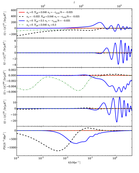
Figure 1: The difference in power spectra between a model with the fiducial parameters set. From the top to the bottom are for the CMB TT, EE, BB, TE angular power spectra, and the matter power spectrum. The red solid line (actually the $x$-axis) indicates the fiducial case. The difference induced by variation in $\alpha_{\mathrm{s}}$(black dashed), $N_{\mathrm{eff}}$(blue solid), and $n_{\mathrm{t}}$(green dash dot) are plotted.

The running of the power spectrum index is included by setting $\alpha_{\mathrm{s}}=-0.022$, and the residuals are shown as black dashed line in Figure 1. The result indicates that, $\alpha_{\mathrm{s}}$ is most sensitive to the scale with $\ell<200$ in the CMB angular spectrum and $\rm{k}<0.1\rm{hMpc}^{-1}$ in the matter power spectrum. Within such scales, the negative $\alpha_{\mathrm{s}}$ can reduce the TT and the matter power spectrum, which is expected for solving the problem in tensor-to-scalar ratio. As reported in Ref.[25], when $\alpha_{\mathrm{s}}=-0.022\pm 0.01~{}(68\%)$, the constraints relax to $r_{0.002}<0.26$, which indicates a possible way to relax the tension.

The parameter $N_{\mathrm{eff}}$ has great effect on smaller scales of the power spectrum. The Standard Model value is $N_{\mathrm{eff}}=3.046$ [47], we plot the difference result for the case $N_{\mathrm{eff}}=3.5$ as shown by the blue solid line in Figure 1. $N_{\mathrm{eff}}$ affects the peaks of BAO, both on the position and the amplitude [35, 36], which is also clearly shown in our figure. A large $N_{\mathrm{eff}}$ causes the suppression on the small scales of the scaler power spectrum. With a large $n_{\mathrm{s}}$, the scalar power spectrum increases at the scales both larger and smaller than the pivot scale of $k=0.05\mathrm{Mpc}^{-1}$. The increased power compensates the suppression at small scales and also reduces tensor-to-scaler ratio at large scales, which can help reduce the tension of $r_{\mathrm{0.002}}$.

The green dashed-dot line in Figure 1 shows the difference between a model with $n_{\mathrm{t}}$ following the consistency relation and a model where this relation is broken, with $n_{\mathrm{t}}=0.3$. It is shown that the variation of $n_{\mathrm{t}}$ mainly affects the large scales of the BB power spectrum.

From the above discussions we see how each parameter affects the CMB and matter power spectra differently, and how it could help to alleviate the tension in the tensor-to-scalar ratio. However, there are still degeneracy and correlation between the effects of various parameters, and the constraints also depends on the priors, so the actual result is more complicated. We perform a global fitting with complete parameter space, and flat prior, to explore the best way to solve the problem.

3 The global fitting

Table 1: Cosmological parameters used in our analysis. For each of them, we list the symbol, prior range and the summary definition. Flat priors are assumed for all parameters.

Table 2: The results of the global fitting with different datasets. For each of the fitting, we consider both imposing and not imposing the inflation consistency relation. Without the consistency relation, $n_{\mathrm{t}}$ is constrained by MCMC as a free parameter. The error are the $68\%$ marginalized limits. The columns with label “Planck + WP” indicate the results obtained with only the Planck and WMAP datasets; the columns with label “+ BICEP” indicate the result of “Planck + WP + BICEP”; while “+ BAO” indicate the results of “Planck + WP + BICEP + BAO”.

We use the CosmoMC code [46] to explore the parameter space and obtain limits on cosmological parameters. In our MCMC simulations, about 500000 samples are collected with 200 chains. The first $1/3$ of the samples is used for burning and not used for the final analysis.

In addition to the BICEP2 data [1], we use the Planck CMB temperature data [25], the WMAP 9 year CMB polarization data [41, 42], and the BAO data from the SDSS DR9 [43], SDSS DR7 [44] and 6dF [45] in our cosmological parameter fitting. For clarity, we use the following labels to denote the different datasets,

• Planck+WP: The Planck high-$\ell$, low-$\ell$ temperature power data[25], and the WMAP9 polarization power data[41, 42] are adopted in the fitting;

• Planck+WP+BICEP: Beside the Planck and WMAP datasets, the BICEP2 data[1, 2] is also included;

• Planck+WP+BICEP+BAO: Beside the CMB measurement data, the BAO data from SDSS DR9[43], SDSS DR7[44], and 6dF[45] are also include in the fitting.

The definition and prior range of some important parameters are listed in Table 1. For most of the parameters, the flat priors are used as in the Planck analysis[25]. Beside the 6 parameters characterizing the simplest inflationary $\Lambda$CDM model, $\Omega_{\mathrm{c}}h^{2}$, $\Omega_{\mathrm{b}}h^{2}$, $\tau$, $\theta_{\mathrm{MC}}$, $A_{\mathrm{s}}$ and $n_{\mathrm{s}}$, we also include the running of scalar power spectrum index $\alpha_{\mathrm{s}}$ and the parameters related with the neutrinos, such as the effective number of neutrinos $N_{\mathrm{eff}}$ and the sum of physical masses of standard neutrinos $\Sigma\mathrm{m_{\nu}}$. Because the evolution of sterile neutrinos is significantly different, it is explored as an extra case, by including one more parameter, $m_{\nu,\,\mathrm{sterile}}^{\mathrm{eff}}$, the effective mass of the sterile neutrinos. When we ignore the single field slow-roll consistency relation, $n_{\mathrm{t}}$ is set to a fixed value, which can be positive or negative, allowing for both red and blue tilt. For comparison, we also run a set of MCMC chains, with $n_{\mathrm{t}}$ following the consistency relation.

4 Results and discussion

The values of the parameters constrained with our global fitting are listed in Table 2. For comparison, the best fits of different datasets with $n_{\mathrm{t}}$ as a free parameter and $n_{\mathrm{t}}=-r_{\mathrm{0.05}}/8$ following the consistency relation are all listed in Table 2.

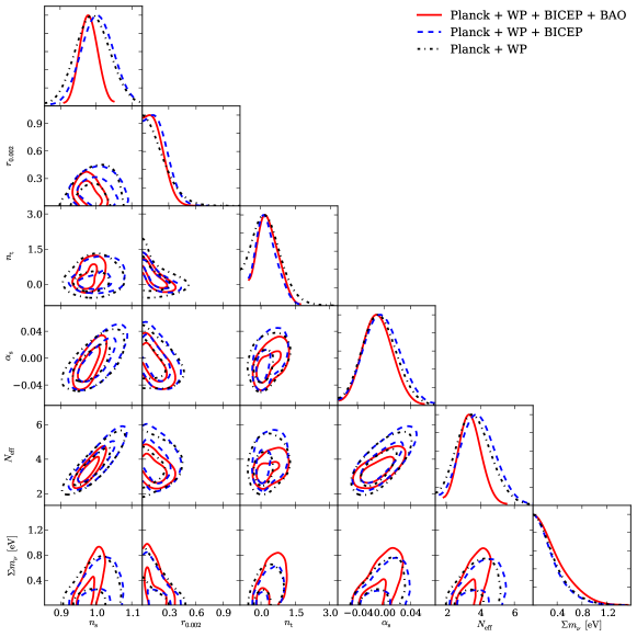
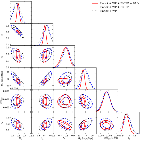
Figure 2: The joint 1d and 2d probability distribution of cosmological parameters. The inner and outer contours represent the $68\%$ and the $95\%$ confidence levels respectively. Top: the primordial power spectrum parameters and the neutrino parameters $N_{\mathrm{eff}}$ and $\Sigma\mathrm{m_{\nu}}$, Bottom: other cosmological parameters. The consistency relation is not imposed.

We plot the 2-dimensional contours and 1-dimensional probability distribution of cosmological parameters with different data sets in Fig.2. The Planck+WMAP constraints are plotted in black dash-dot lines, the constraint with additional BICEP data are plotted with blue dash lines, and the constraint also with BAO are plotted in red solid lines. Here we do not impose the consistency relation, and $n_{t}$ is taken as a free parameter. From these plots, we find that with the inclusion of the neutrino parameters, there is no significant conflict between the result of including and excluding the BICEP2 data set, the allowed parameter range or region overlap with each other in these two cases. The constraints also become tighter with the additional BAO datasets included. With only the Planck and WMAP9 datasets, $r_{\mathrm{0.002}}<0.16(0.36)$ with $68\%(95\%)$ marginalized limits. The constraints are different from that reported by Planck Collaboration et al. [25], since some extra free parameters are included in our global fitting, such as $n_{\mathrm{t}}$, $\alpha_{\mathrm{s}}$, $N_{\mathrm{eff}}$ and $\Sigma m_{\mathrm{\mu}}$. Now, with the additional of the BICEP2 data, we find $r_{\mathrm{0.002}}=0.16_{-0.12}^{+0.06}$, and $r_{\mathrm{0.002}}=0.14_{-0.11}^{+0.05}$ with both the BICEP2 and the BAO datasets included. The results are all consistent with each other.

In the above we have taken $n_{t}$ as a free parameter without imposing the consistency relation. If we do impose the consistency relation in our fitting, the $68\%$ marginalized limits are $r_{\mathrm{0.002}}<0.24$ with only Planck and WMAP9 datasets; $r_{\mathrm{0.002}}=0.24_{-0.07}^{+0.05}$ with BICEP2 data included; and $r_{\mathrm{0.002}}=0.22_{-0.06}^{+0.04}$ with both BICEP2 and BAO datasets included. The results are all consistent with Ref.[1].

These results show that the tension between the BICEP and Planck data is removed by including $n_{\mathrm{t}}$, $\alpha_{\mathrm{s}}$ and the neutrino parameters as free parameters in the global fitting. Below we investigate which parameters are responsible for this.

4.1 $n_{\mathrm{t}}$ is not the key parameter

As discussed in Sect. 2, $n_{\mathrm{t}}$ has significant effect on the BB power spectrum, but not on the TT or the matter power spectrum. The results of our global fitting with different data sets also indicate that the constraints on $n_{\mathrm{t}}$ become better with the inclusdion of BICEP2 data set, but the BAO data set does not help to improve the constraint on it.

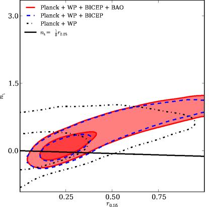
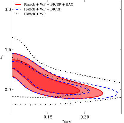
Figure 3: Left: The joint probability of $n_{\mathrm{t}}$ and $r_{\mathrm{0.05}}$, the black solid line represents the single-field inflation consistency relation $n_{\mathrm{t}}=-r_{\mathrm{0.05}}/8$. Right: The joint probability of $n_{\mathrm{t}}$ and $r_{\mathrm{0.002}}$. The inner and outer contours represent the $68\%$ and $95\%$ confidence levels respectively.

The left panel of Figure 3 shows the joint probability of $n_{\mathrm{t}}$ and $r_{\mathrm{0.05}}$, when the consistency relation is not imposed. For reference, we also plot the consistence relation with the black solid line in the same figure. The consistency relation also forces $n_{\mathrm{t}}$ to be negative, so the tensor spectrum has a red tilt. From the figure we see that the global fitting results are still consistent with the consistency relation. Although the result favors a blue tilt in the tensor spectrum slightly, it is not as significant as reported in Ref.[33].

In the right panel of Figure 3, we show the contours for $r_{0.002}$ and $n_{\mathrm{t}}$, note here $n_{\mathrm{t}}$ is measured around $k=0.05h/\mbox{\rm\,Mpc}$. If $r_{0.002}<0.11$[25], it would be easy to get a larger blue tilt tensor power spectrum. However, when the consistency relation is imposed, it forces $n_{\mathrm{t}}$ to a small negative value, and yields a large $r_{0.002}$. In our global fitting, the constraints with flat prior result in a slightly smaller $r_{0.002}=0.14^{+0.05}_{-0.11}$, while with the consistency relation imposed, $r_{0.002}=0.22^{+0.05}_{-0.06}$, which is consistent with the results reported in Ref.[1].

We see the results obtained with the different data sets are generally consistent with each other, either with or without the consistency relation imposed. Including $n_{\mathrm{t}}$ as a free parameter is not a necessary condition for solving the tension, but the value of $r_{\mathrm{0.002}}$ is correlated with the prior of $n_{\mathrm{t}}$.

4.2 $\alpha_{\mathrm{s}}$ helps little

In the paper of BICEP2 Collaboration et al. [1], $\alpha_{\mathrm{s}}$ is introduced to reduce the tension in $r_{0.002}$. According to their analysis, a negative $\alpha_{\mathrm{s}}\sim-0.022$ is needed for suppressing the scalar power spectrum. In our fitting, the $\alpha_{\mathrm{s}}$ is constrained to $\alpha_{\mathrm{s}}=-0.0054_{-0.0217}^{+0.0162}(68\%)$ with Planck and WMAP9 data; $\alpha_{\mathrm{s}}=-0.0011_{-0.0241}^{+0.0187}(68\%)$ with BICEP2 data included; and $\alpha_{\mathrm{s}}=-0.0086_{-0.0189}^{+0.0148}(68\%)$ with all the datasets included. The values of $\alpha_{\mathrm{s}}$ for different datasets agree within error range, and also consistent with $\alpha_{\mathrm{s}}=0$. Such a small $\alpha_{\mathrm{s}}$ can not give enough suppression on scalar perturbation for solving the tension.

In the case of $n_{\mathrm{t}}$ following the consistency relation assumption, the $\alpha_{\mathrm{s}}$ is constrained to $\alpha_{\mathrm{s}}=-0.0133_{-0.0162}^{+0.0129}(68\%)$ with all the datasets included. The non-zero results indicate that the $\alpha_{\mathrm{s}}$ is still helpful for suppressing the scalar power spectrum and alleviating the $r_{\mathrm{0.002}}$ tension, at least when the consistency relation is imposed.

However, the large value of $\alpha_{\mathrm{s}}\sim-0.02$ leads to small value of e-folds number in slow roll inflation, which is unacceptable in our universe [26, 27],. In this case, $\alpha_{\mathrm{s}}$ is not a good choice for solving the problem of tension between Planck and BICEP2.

4.3 The neutrinos helps much

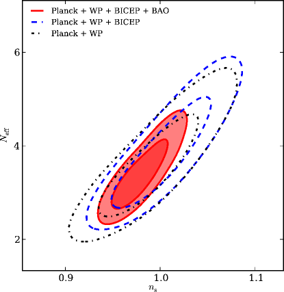
Figure 4: This plot shows the joint probability of $N_{\mathrm{eff}}$ and $n_{\mathrm{s}}$ constrained from our MCMC global fitting, by using different datasets, without considering the consistency relation. The inner and outer contours represent the $68\%$ and $95\%$ confidence levels respectively.

The neutrinos mainly affect the scalar and tensor power spectrum on small scales. According to the analysis in Bashinsky and Seljak [35], Hou et al. [36], Lesgourgues et al. [48], $N_{\mathrm{eff}}$ mainly affects the scales of BAO peaks, which are out of the scale range of BICEP2 data. So the constraint on neutrinos comes mainly from the Planck data sets and BAO data sets. As shown in the Figure 2, with neutrino parameters in the fit, the contours do not change much when the BICEP2 data is added. Because the neutrinos are still relativistic at the epoch of Recombination, $\Sigma\mathrm{m_{\nu}}$ only has a small effect on the primary power spectrum and it is hard to be constrained. We find that, $\Sigma\mathrm{m_{\nu}}$ is constrained to be $<0.29\mathrm{ev}$ with the Planck and the WMAP9 data; $<0.27\mathrm{eV}$ with the BICEP2 data included; and $<0.37\mathrm{eV}$ with both the BICEP2 and the BAO data included.

The $N_{\mathrm{eff}}$ is a more interesting parameter in this case. It is constrained to be $N_{\mathrm{eff}}=3.66^{+0.61}_{-0.92}$ with the Planck and the WMAP9 data only; $N_{\mathrm{eff}}=3.93^{+0.66}_{-0.93}$ with the BICEP2 data added; and $N_{\mathrm{eff}}=3.43^{+0.39}_{-0.58}$ with the BICEP2 and the BAO datasets included. We get larger $N_{\mathrm{eff}}$ than that in the Standard Model. The result is consistent with recent CMB measurement [49, 50, 51, 52, 41, 36, 25]. Such a large $N_{\mathrm{eff}}$ is expected for solving the $r_{\mathrm{0.002}}$ tension. Because of the suppression of the large $N_{\mathrm{eff}}$ on small scales, a large $n_{\mathrm{s}}$ becomes acceptable, and the large $n_{\mathrm{s}}$ can help solving the tension problem on large scale. Such a degeneration can be found through the 2d contours of $N_{\mathrm{eff}}$ and $n_{\mathrm{s}}$ in Figure 4. Without considering BAO and BICEP2 data, $n_{\mathrm{s}}=0.99_{-0.04}^{+0.03}$ which is larger than $1$ within $68\%$ marginalized confidence interval. With the BICEP2 data added, the $n_{\mathrm{s}}$ is constrained to be $1.01^{+0.03}_{-0.04}$. By including the BAO and BICEP2 data, $n_{\mathrm{s}}=0.98_{-0.02}^{+0.02}$ which is still consistent with $n_{\mathrm{s}}<1$.

The large $N_{\mathrm{eff}}$ could be explained by including extra neutrinos such as the sterile neutrinos, neutrino/anti-neutrino asymmetry and/or any other light relics in the universe. In the case of sterile neutrinos, the related parameters, $m_{\nu,\,\mathrm{sterile}}^{\mathrm{eff}}$ and $N_{\mathrm{eff}}$ are constrained to $m_{\nu,\,\mathrm{sterile}}^{\mathrm{eff}}<0.79$, $N_{\mathrm{eff}}<4.30$ with only the Planck and the WMAP9 datasets; $m_{\nu,\,\mathrm{sterile}}^{\mathrm{eff}}<0.75$, $N_{\mathrm{eff}}=4.19^{+0.36}_{-1.08}$ with the BICEP2 data added; and $m_{\nu,\,\mathrm{sterile}}^{\mathrm{eff}}=0.53^{+0.21}_{-0.42}$, $N_{\mathrm{eff}}<4.05$ with the BICEP2 and the BAO datasets both included. And in such case, $r_{\mathrm{0.002}}$ is constrained to $r_{\mathrm{0.002}}<0.23$ with the Planck and the BICEP2 datasets; $r_{\mathrm{0.002}}=0.18^{+0.08}_{-0.11}$ with the BICEP2 datasets included; and $r_{\mathrm{0.002}}=0.19^{+0.08}_{-0.09}$ with the BICEP2 and the BAO datasets both included. The consistent constraints on $r_{\mathrm{0.002}}$ indicate the alleviation of the tension between different datasets.

Using sterile neutrinos to alleviate the tension between the Planck data set and other data set has also been discussed in Zhang et al. [37], Dvorkin et al. [39]. Their conclusion are in agreement with ours. With the complete exploration of the parameter space, we also find that including neutrino parameters plays an important role in solving the tension.

5 conclusion

In this paper, we explore various ways to alleviate apparent tension between the constraints on the inflationary tensor-to-scalar ratio $r_{\mathrm{0.002}}$ obtained from the BICEP2 data and the Planck data. The fittings are performed with the Planck CMB temperature data[25] and the WMAP 9 year CMB polarization data[41, 42], with/out the newly published BICEP2 CMB B-mode data. we also use the BAO data from SDSS DR9[43], SDSS DR7[44] and 6dF[45], to help breaking some parameter degeneracy and improve the precision of the model.. By setting $\alpha_{\mathrm{s}}$, $n_{\mathrm{t}}$ and neutrino parameters as free parameters, the resulting constraints on $r_{\mathrm{0.002}}$ from different data sets are found to be consistent with each other,

With all the datasets included, we obtain marginalized $68\%$ bounds on some interested parameters as follows:

$$r_{\mathrm{0.002}} = 0.14_{-0.11}^{+0.05},$$ (4)

$$n_{\mathrm{s}} = 0.98_{-0.02}^{+0.02},$$ (5)

$$\alpha_{\mathrm{s}} = -0.0086_{-0.0189}^{+0.0148},$$ (6)

$$n_{\mathrm{t}} = 0.35_{-0.47}^{+0.28}.$$ (7)

The value of $r_{\mathrm{0.002}}$ obtained in this work is smaller than that reported by the BICEP2 team, due to its dependence on $n_{\mathrm{t}}$, which is constrained to be positive(blue tensor tilt), but a flat or even red tilt is still consistent with the data. Further more, the results do not deviate from the consistency relation, even if we ignore the relation in the fitting. Because the consistency relation restricts $n_{\mathrm{t}}$ to a lower value, it breaks the degeneracy between $n_{\mathrm{t}}$ and $r_{0.002}$. By applying this relation as a prior in the fitting, a tighter constraint on $r_{0.002}$ is obtained, $r_{0.002}=0.22_{-0.06}^{+0.05}$.

Although the tension is alleviated by including $\alpha_{\mathrm{s}}$, $n_{\mathrm{t}}$ and neutrino parameters as free parameters, we find that $\alpha_{\mathrm{s}}$ and $n_{\mathrm{t}}$ are not the key parameters. The scalar running $\alpha_{\mathrm{s}}$ is still consistent with $0$, this indicates that including $\alpha_{\mathrm{s}}$ may not be the best choice for solving the $r_{0.002}$ tension; The results are consistent with different data sets, with or without $n_{\mathrm{t}}$ as a free parameter, which indicates that $n_{\mathrm{t}}$ is not necessary for solving the $r_{\mathrm{0.002}}$ tension problem. Finally, the effective number of neutrinos $N_{\mathrm{eff}}$, constrained to $3.43_{-0.58}^{+0.39}$, appears to be the most important parameter for this problem.

We also check our result with the sterile neutrinos. By including all the data sets, $N_{\mathrm{eff}}$ is constrained to be $<4.05$, $m_{\nu,\,\mathrm{sterile}}^{\mathrm{eff}}$ is constrained to be $0.53^{+0.21}_{-0.42}$, and in this case, $r_{\mathrm{0.002}}$ is constrained to be $0.19^{+0.08}_{-0.09}$.

References

- BICEP2 Collaboration et al. [2014a] BICEP2 Collaboration, P. A. R. Ade, R. W. Aikin, D. Barkats, S. J. Benton, C. A. Bischoff, J. J. Bock, J. A. Brevik, I. Buder, E. Bullock, et al., ArXiv e-prints (2014a), 1403.3985.
- BICEP2 Collaboration et al. [2014b] BICEP2 Collaboration, P. A. R. Ade, R. W. Aikin, M. Amiri, D. Barkats, S. J. Benton, C. A. Bischoff, J. J. Bock, J. A. Brevik, I. Buder, et al., ArXiv e-prints (2014b), 1403.4302.
- Liu et al. [2014] H. Liu, P. Mertsch, and S. Sarkar, ArXiv e-prints (2014), 1404.1899.
- Mortonson and Seljak [2014] M. J. Mortonson and U. Seljak, ArXiv e-prints (2014), 1405.5857.
- Flauger et al. [2014] R. Flauger, J. C. Hill, and D. N. Spergel, ArXiv e-prints (2014), 1405.7351.
- Starobinsky [1980] A. A. Starobinsky, Physics Letters B 91, 99 (1980).
- Guth [1981] A. H. Guth, Physical Review D 23, 347 (1981).
- Albrecht and Steinhardt [1982] A. Albrecht and P. J. Steinhardt, Physical Review Letters 48, 1220 (1982).
- Linde [1982] A. D. Linde, Physics Letters B 108, 389 (1982).
- Kosowsky and Turner [1995] A. Kosowsky and M. S. Turner, Physical Review D 52, 1739 (1995), astro-ph/9504071.
- Hertzberg [2014] M. P. Hertzberg, ArXiv e-prints (2014), 1403.5253.
- Choudhury and Mazumdar [2014] S. Choudhury and A. Mazumdar, ArXiv e-prints (2014), 1403.5549.
- Ma and Wang [2014] Y.-Z. Ma and Y. Wang, ArXiv e-prints (2014), 1403.4585.
- Gao and Gong [2014] Q. Gao and Y. Gong, ArXiv e-prints (2014), 1403.5716.
- Xia et al. [2014] J.-Q. Xia, Y.-F. Cai, H. Li, and X. Zhang, ArXiv e-prints (2014), 1403.7623.
- Cai et al. [2014] Y.-F. Cai, J.-O. Gong, and S. Pi, ArXiv e-prints (2014), 1404.2560.
- Zhao et al. [2014] W. Zhao, C. Cheng, and Q.-G. Huang, ArXiv e-prints (2014), 1403.3919.
- Zhao and Grishchuk [2010] W. Zhao and L. P. Grishchuk, Physical Review D 82, 123008 (2010), 1009.5243.
- Bhattacharya et al. [2014] K. Bhattacharya, J. Chakrabortty, S. Das, and T. Mondal, ArXiv e-prints (2014), 1408.3966.
- Nozari and Rashidi [2014] K. Nozari and N. Rashidi, ArXiv e-prints (2014), 1408.3192.
- Elizalde et al. [2014] E. Elizalde, S. D. Odintsov, E. O. Pozdeeva, and S. Y. Vernov, ArXiv e-prints (2014), 1408.1285.
- Dine and Stephenson-Haskins [2014] M. Dine and L. Stephenson-Haskins, ArXiv e-prints (2014), 1408.0046.
- Anchordoqui [2014] L. A. Anchordoqui, ArXiv e-prints (2014), 1407.8105.
- Maity and Saha [2014] D. Maity and P. Saha, ArXiv e-prints (2014), 1407.7692.
- Planck Collaboration et al. [2013] Planck Collaboration, P. A. R. Ade, N. Aghanim, C. Armitage-Caplan, M. Arnaud, M. Ashdown, F. Atrio-Barandela, J. Aumont, C. Baccigalupi, A. J. Banday, et al., ArXiv e-prints (2013), 1303.5076.
- Contaldi et al. [2014] C. R. Contaldi, M. Peloso, and L. Sorbo, ArXiv e-prints (2014), 1403.4596.
- Easther and Peiris [2006] R. Easther and H. V. Peiris, Journal of Cosmology and Astroparticle Physics 9, 010 (2006), astro-ph/0604214.
- Wang and Xue [2014] Y. Wang and W. Xue, ArXiv e-prints (2014), 1403.5817.
- Ashoorioon et al. [2014] A. Ashoorioon, K. Dimopoulos, M. M. Sheikh-Jabbari, and G. Shiu, ArXiv e-prints (2014), 1403.6099.
- Abazajian et al. [2014] K. N. Abazajian, G. Aslanyan, R. Easther, and L. C. Price, ArXiv e-prints (2014), 1403.5922.
- Gong [2014] J.-O. Gong, ArXiv e-prints (2014), 1403.5163.
- Brandenberger et al. [2014] R. H. Brandenberger, A. Nayeri, and S. P. Patil, ArXiv e-prints (2014), 1403.4927.
- Gerbino et al. [2014] M. Gerbino, A. Marchini, L. Pagano, L. Salvati, E. Di Valentino, and A. Melchiorri, ArXiv e-prints (2014), 1403.5732.
- Wu et al. [2014] F. Wu, Y. Li, Y. Lu, and X. Chen, ArXiv e-prints (2014), 1403.6462.
- Bashinsky and Seljak [2004] S. Bashinsky and U. Seljak, Physical Review D 69, 083002 (2004), astro-ph/0310198.
- Hou et al. [2013] Z. Hou, R. Keisler, L. Knox, M. Millea, and C. Reichardt, Physical Review D 87, 083008 (2013), 1104.2333.
- Zhang et al. [2014a] J.-F. Zhang, Y.-H. Li, and X. Zhang, ArXiv e-prints (2014a), 1403.7028.
- Archidiacono et al. [2014] M. Archidiacono, N. Fornengo, S. Gariazzo, C. Giunti, S. Hannestad, and M. Laveder, ArXiv e-prints (2014), %****␣bicep2.bbl␣Line␣325␣****1404.1794.
- Dvorkin et al. [2014] C. Dvorkin, M. Wyman, D. H. Rudd, and W. Hu, ArXiv e-prints (2014), 1403.8049.
- Zhang et al. [2014b] J.-F. Zhang, J.-J. Geng, and X. Zhang, ArXiv e-prints (2014b), 1408.0481.
- Hinshaw et al. [2013] G. Hinshaw, D. Larson, E. Komatsu, D. N. Spergel, C. L. Bennett, J. Dunkley, M. R. Nolta, M. Halpern, R. S. Hill, N. Odegard, et al., ASTROPHYSICAL JOURNAL SUPPLEMENT SERIES 208, 19 (2013), 1212.5226.
- Bennett et al. [2013] C. L. Bennett, D. Larson, J. L. Weiland, N. Jarosik, G. Hinshaw, N. Odegard, K. M. Smith, R. S. Hill, B. Gold, M. Halpern, et al., The Astrophysical Journal Supplement Series 208, 20 (2013), 1212.5225.
- Anderson et al. [2014] L. Anderson, É. Aubourg, S. Bailey, F. Beutler, V. Bhardwaj, M. Blanton, A. S. Bolton, J. Brinkmann, J. R. Brownstein, A. Burden, et al., Monthly Notices of the Royal Astronomical Society 441, 24 (2014), 1312.4877.
- Padmanabhan et al. [2012] N. Padmanabhan, X. Xu, D. J. Eisenstein, R. Scalzo, A. J. Cuesta, K. T. Mehta, and E. Kazin, Monthly Notices of the Royal Astronomical Society 427, 2132 (2012), 1202.0090.
- Beutler et al. [2011] F. Beutler, C. Blake, M. Colless, D. H. Jones, L. Staveley-Smith, L. Campbell, Q. Parker, W. Saunders, and F. Watson, Monthly Notices of the Royal Astronomical Society 416, 3017 (2011), 1106.3366.
- Lewis and Bridle [2002] A. Lewis and S. Bridle, Physical Review D 66, 103511 (2002), astro-ph/0205436.
- Mangano et al. [2005] G. Mangano, G. Miele, S. Pastor, T. Pinto, O. Pisanti, and P. D. Serpico, Nuclear Physics B 729, 221 (2005), hep-ph/0506164.
- Lesgourgues et al. [2013] J. Lesgourgues, G. Mangano, G. Miele, and S. Pastor, Neutrino Cosmology (2013).
- Komatsu et al. [2011] E. Komatsu, K. M. Smith, J. Dunkley, C. L. Bennett, B. Gold, G. Hinshaw, N. Jarosik, D. Larson, M. R. Nolta, L. Page, et al., The Astrophysical Journal Supplement Series 192, 18 (2011), 1001.4538.
- Dunkley et al. [2011] J. Dunkley, R. Hlozek, J. Sievers, V. Acquaviva, P. A. R. Ade, P. Aguirre, M. Amiri, J. W. Appel, L. F. Barrientos, E. S. Battistelli, et al., The Astrophysical Journal 739, 52 (2011), 1009.0866.
- Keisler et al. [2011] R. Keisler, C. L. Reichardt, K. A. Aird, B. A. Benson, L. E. Bleem, J. E. Carlstrom, C. L. Chang, H. M. Cho, T. M. Crawford, A. T. Crites, et al., The Astrophysical Journal 743, 28 (2011), 1105.3182.
- Archidiacono et al. [2011] M. Archidiacono, E. Calabrese, and A. Melchiorri, Physical Review D 84, 123008 (2011), 1109.2767.